
Generating Cubes and Cutouts from TESS FFIs#
Learning Goals#
By the end of this tutorial, you will:
Learn about the two TESS full frame image (FFI) types: SPOC and TICA.
Learn the structure of a TICA FFI.
Learn how to retrieve and download TESS FFIs using
astroquery.mast.Observations.Learn how to generate cubes from TESS FFIs with astrocut’s
CubeFactoryandTicaCubeFactory.Learn how to generate cutouts from TESS cubes with astrocut’s
CutoutFactory.Learn the structure of a TESS target pixel file (TPF), and therefore an astrocut cutouts file, and how to retrieve and plot the data stored within.
Introduction#
In this tutorial, you will learn the basic functionality of astrocut’s CubeFactory, TicaCubeFactory, and CutoutFactory. These 3 tools allow users to generate cubes and cutouts of TESS images. TESS image cubes are stacks of TESS full frame images (TESS FFIs) which are formatted to allow users to make cutouts with CutoutFactory. These cutouts are sub-images that will only contain your region of interest, to make analysis easier.
The process of generating cubes, and making cutouts from them, mimicks the web-based TESSCut service. This tutorial will teach you to make cubes and cutouts that are customized for your specific use-cases, while also giving insight to how TESSCut calls upon astrocut to create cutouts.
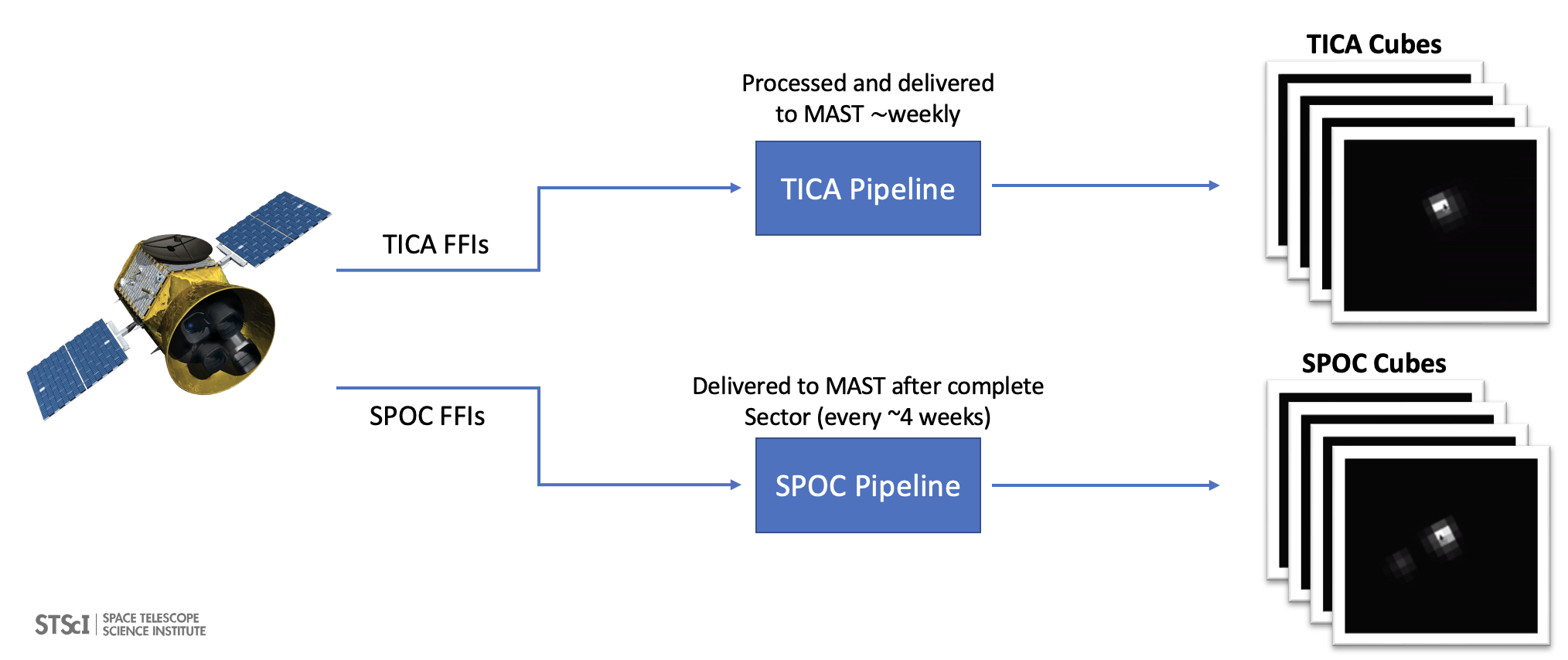
As in the TESSCut service, there are two different TESS FFI product types you can work with in this notebook. These two product types are the TESS mission-provided, Science Processing Operations Center (SPOC) FFIs, and the TESS Image CAlibrator (TICA) FFIs. Both are available via astroquery.mast.Observations, and both have different use-cases. The TICA products offer the latest sector observations due to their faster delivery cadence, and can be available up to 3 times sooner than their SPOC counterparts. As such, for those who are working with time-sensitive observations, TICA may be the best option for generating your cutouts. Note that the SPOC and TICA products are processed through different pipelines and thus have different pixel values and WCS solutions. Please refer to the SPOC pipeline paper and the TICA pipeline paper for more information on the differences and similarities between the SPOC and TICA products.
The workflow for this notebook consists of:
Retrieving and Downloading the FFIs
Retrieving the FFIs
Downloading the FFIs
Inspecting the FFIs
Creating a Cube
Creating the Cutouts
Exercise: Generate Cutouts for TIC 2527981 Sector 27 SPOC Products
Resources
Imports#
Below is a list of the packages used throughout this notebook, and their use-cases. Please ensure you have the recommended version of these packages installed on the environment this notebook has been launched in. See the requirements.txt file for recommended package versions.
astropy.units for unit conversion
matplotlib.pyplot for plotting data
numpy to handle array functions
astrocut CubeFactory for generating cubes out of TESS-SPOC FFIs
astrocut TicaCubeFactory for generating cubes out of TICA FFIs
astrocut CutoutFactory for generating cutouts out of astrocut cubes
astropy.coordinates SkyCoord for creating sky coordinate objects
astropy.io fits for accessing FITS files
astroquery.mast Observations for retrieving and downloading the TESS FFIs
matplotlib.path Path to generate a drawing path for plotting purposes
matplotlib.patches PathPatch to generate a patch that represents the CCD footprint for plotting purposes
%matplotlib inline

import astropy.units as u
import matplotlib.pyplot as plt
import numpy as np

from astrocut import CubeFactory, TicaCubeFactory, CutoutFactory
from astropy.coordinates import SkyCoord
from astropy.io import fits
from astroquery.mast import Observations
from matplotlib.path import Path
from matplotlib.patches import PathPatch
Below are the helper functions we will call for plotting purposes later in the notebook.
def convert_coords(ra, dec):
    """ Wrap the input coordinates `ra` and `dec` around the upper limit of 180
    degrees and convert to radians so that they may be plotted on the Aitoff canvas.

    Parameter(s)
    -----------
    ra : str, int, or float
        The Right Ascension your target lands on, in degrees. May be any object type that
        can be converted to a float, such as a string, or integer.
    dec : str, int, or float
        The Declination your target lands on, in degrees. May be any object type that
        can be converted to a float, such as a string, or integer.

    Returns
    -------
    ra_rad : float
        The Right Ascension of your target in radians.
    dec_rad : float
        The Declination of your target in radians.
    """

    # Make a SkyCoord object out of the RA, Dec
    c = SkyCoord(ra=float(ra)*u.degree, dec=float(dec)*u.degree, frame='icrs')

    # The plotting only works when the coordinates are in radians.
    # And because it's an aitoff projection, we can't
    # go beyond 180 degrees, so let's wrap the RA vals around that upper limit.
    ra_rad = c.ra.wrap_at(180 * u.deg).radian
    dec_rad = c.dec.radian

    return ra_rad, dec_rad

def plot_footprint(coords):
    """ Plots a polygon of 4 vertices onto an aitoff projection on a matplotlib canvas.

    Parameter(s)
    -----------
    coords : list or array of tuples
        An iterable object (can be a list or array) of 5 tuples, each tuple containing the
        RA and Dec (float objects) of a vertice of your footprint. There MUST be 5: 1 for each
        vertice, and 1 to return to the starting point, as PathPatch works with a set of drawing
        instructions, rather than a predetermined shape.

    Returns
    -------
    ax : Matplotlib.pyplot figure object subplot
        The subplot that contains the aitoff projection and footprint drawing.
    """

    assert len(coords) == 5, 'We need 5 sets of coordinates. 1 for each vertice + 1 to return to the starting point.'
    instructions = [Path.MOVETO, Path.LINETO, Path.LINETO, Path.LINETO, Path.CLOSEPOLY]

    # Create the path patch using the `coords` list of tuples and the
    # instructions from above
    c = np.array(coords)
    path = Path(c, instructions)
    ppatch = PathPatch(path, edgecolor='k', facecolor='salmon')

    # Create a matplotlib canvas
    fig = plt.figure(figsize=(12,12))

    # We will be using the `aitoff` projection for a globe canvas
    ax = plt.subplot(111, projection='aitoff')

    # Need grids!
    ax.grid()

    # Add the patch to your canvas
    ax.add_patch(ppatch)

    return ax
Retrieving and Downloading the FFIs#
Before we begin generating cubes and cutouts from TESS FFIs, we must first acquire these FFIs. To do this, we will request and download the FFIs locally using astroquery.mast, or more specifically, the astroquery.mast.Observations tool, which will grant us access to the database that houses the TESS products. This is also how the TESSCut API generates its cutouts.
Retrieving the FFIs#
You can download FFIs for any sector, camera, and CCD type. This notebook will generate cutouts for target TIC 2527981 using TICA FFIs in sector 27, but feel free to substitute a favorite target of your own. To find our target, we will filter with the database criteria: coordinates, target_name, dataproduct_type, and sequence_number.
The coordinates criteria will filter for the coordinates of our target, while the target_name will filter for TICA FFIs and exclude all SPOC FFIs. dataproduct_type ensures we get image observations, and the sequence_number will be used to filter for only sector 27 observations. With this information, let’s compile our query…
# We will pass in the coordinates as a Sky Coord object
coordinates = SkyCoord(289.0979, -29.3370, unit="deg")

obs = Observations.query_criteria(coordinates=coordinates,
                                  target_name='TICA FFI',
                                  dataproduct_type='image',
                                  sequence_number=27)

obs
| intentType | obs_collection | provenance_name | instrument_name | project | filters | wavelength_region | target_name | target_classification | obs_id | s_ra | s_dec | dataproduct_type | proposal_pi | calib_level | t_min | t_max | t_exptime | em_min | em_max | obs_title | t_obs_release | proposal_id | proposal_type | sequence_number | s_region | jpegURL | dataURL | dataRights | mtFlag | srcDen | obsid | objID | objID1 | distance |
|---|---|---|---|---|---|---|---|---|---|---|---|---|---|---|---|---|---|---|---|---|---|---|---|---|---|---|---|---|---|---|---|---|---|---|
| str7 | str4 | str4 | str10 | str4 | str4 | str7 | str8 | str1 | str25 | float64 | float64 | str5 | str17 | int64 | float64 | float64 | float64 | float64 | float64 | str1 | float64 | str3 | str1 | int64 | str117 | str1 | str1 | str6 | bool | float64 | str8 | str9 | str9 | float64 |
| science | HLSP | TICA | Photometer | TESS | TESS | Optical | TICA FFI | -- | hlsp_tica_s0027-cam1-ccd4 | 292.5180823224232 | -33.62274382166828 | image | Michael Fausnaugh | 3 | 59035.77807636512 | 59060.13917620387 | 475.2 | 600.0 | 1000.0 | -- | 59246.0 | N/A | -- | 27 | POLYGON 298.489297 -26.919235 301.396094 -38.579035 285.694884 -40.219585 285.275975 -28.732615 298.489297 -26.919235 | -- | -- | PUBLIC | False | nan | 96814766 | 185636258 | 185636258 | 0.0 |
This is the sector 27 FFI that contains TIC2527981. Note that the s_ra and s_dec listed above are the center of the CCD that contains the target, not the coordinates of the target itself.
To demonstrate this, let’s plot the s_region metadata, the s_ra and s_dec coordinates, and the input coordinates of our target to see where it lands relative to sector 27, camera 1, CCD 4.
# Extract the polygon vertices, then store them in separate lists
polygon = obs['s_region'][0]
split = polygon.split(' ')
# Removing the "POLYGON" string
split.pop(0)
# Storing the RAs and Decs separately
ras, decs = split[::2], split[1::2]

# Now we convert our RAs/Decs into radians and wrap them around 180 degrees
coords = []
for ra, dec in zip(ras, decs):
    ra_rad, dec_rad = convert_coords(ra, dec)
    coords.append((ra_rad, dec_rad))

# We use Matplotlib's Path and PathPatch to plot the footprint of sector 27, camera 1, CCD 4
ax = plot_footprint(coords)

# Now let's plot our input target's RA, Dec on top of the footprint to see its relative position
target_ra, target_dec = coordinates.ra.degree, coordinates.dec.degree
target_coords = convert_coords(target_ra, target_dec)
ax.scatter(target_coords[0], target_coords[1], color='k', label='target coords')

# And lastly, let's plot the s_ra and s_dec coordinates to see what they represent
s_coords = convert_coords(obs['s_ra'][0], obs['s_dec'][0])
ax.scatter(s_coords[0], s_coords[1], color='grey', label='s_ra, s_dec')

ax.set_title('Sector 27, Camera 1, CCD 4 Footprint' + '\n' + ' ')
plt.legend()
plt.show()
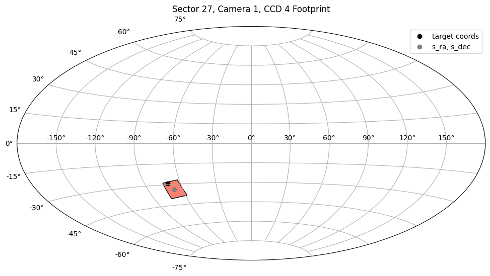
The plot above shows the positioning of TIC 2527981 relative to sector 27, camera 1, CCD 4. You can see that it is more or less on the edge of this CCD, and not the center. Note also that the s_ra and s_dec fall exactly in the center of the CCD.
From this observation we can now retrieve the corresponding TICA products (FFIs). Let’s use the get_product_list method to retrieve these FFIs.
products = Observations.get_product_list(obs)
products
| obsID | obs_collection | dataproduct_type | obs_id | description | type | dataURI | productType | productGroupDescription | productSubGroupDescription | productDocumentationURL | project | prvversion | proposal_id | productFilename | size | parent_obsid | dataRights | calib_level |
|---|---|---|---|---|---|---|---|---|---|---|---|---|---|---|---|---|---|---|
| str8 | str4 | str5 | str59 | str4 | str1 | str95 | str7 | str1 | str1 | str1 | str4 | str1 | str3 | str64 | int64 | str8 | str6 | int64 |
| 96582260 | HLSP | image | hlsp_tica_tess_ffi_s0027-o1-00116470-cam1-ccd4_tess_v01_img | FITS | D | mast:HLSP/tica/s0027/cam1-ccd4/hlsp_tica_tess_ffi_s0027-o1-00116470-cam1-ccd4_tess_v01_img.fits | SCIENCE | -- | -- | -- | TICA | 1 | N/A | hlsp_tica_tess_ffi_s0027-o1-00116470-cam1-ccd4_tess_v01_img.fits | 17795520 | 96814766 | PUBLIC | 4 |
| 96582824 | HLSP | image | hlsp_tica_tess_ffi_s0027-o1-00116471-cam1-ccd4_tess_v01_img | FITS | D | mast:HLSP/tica/s0027/cam1-ccd4/hlsp_tica_tess_ffi_s0027-o1-00116471-cam1-ccd4_tess_v01_img.fits | SCIENCE | -- | -- | -- | TICA | 1 | N/A | hlsp_tica_tess_ffi_s0027-o1-00116471-cam1-ccd4_tess_v01_img.fits | 17795520 | 96814766 | PUBLIC | 4 |
| 96584339 | HLSP | image | hlsp_tica_tess_ffi_s0027-o1-00116472-cam1-ccd4_tess_v01_img | FITS | D | mast:HLSP/tica/s0027/cam1-ccd4/hlsp_tica_tess_ffi_s0027-o1-00116472-cam1-ccd4_tess_v01_img.fits | SCIENCE | -- | -- | -- | TICA | 1 | N/A | hlsp_tica_tess_ffi_s0027-o1-00116472-cam1-ccd4_tess_v01_img.fits | 17795520 | 96814766 | PUBLIC | 4 |
| 96582627 | HLSP | image | hlsp_tica_tess_ffi_s0027-o1-00116473-cam1-ccd4_tess_v01_img | FITS | D | mast:HLSP/tica/s0027/cam1-ccd4/hlsp_tica_tess_ffi_s0027-o1-00116473-cam1-ccd4_tess_v01_img.fits | SCIENCE | -- | -- | -- | TICA | 1 | N/A | hlsp_tica_tess_ffi_s0027-o1-00116473-cam1-ccd4_tess_v01_img.fits | 17795520 | 96814766 | PUBLIC | 4 |
| 96584033 | HLSP | image | hlsp_tica_tess_ffi_s0027-o1-00116474-cam1-ccd4_tess_v01_img | FITS | D | mast:HLSP/tica/s0027/cam1-ccd4/hlsp_tica_tess_ffi_s0027-o1-00116474-cam1-ccd4_tess_v01_img.fits | SCIENCE | -- | -- | -- | TICA | 1 | N/A | hlsp_tica_tess_ffi_s0027-o1-00116474-cam1-ccd4_tess_v01_img.fits | 17795520 | 96814766 | PUBLIC | 4 |
| 96583083 | HLSP | image | hlsp_tica_tess_ffi_s0027-o1-00116475-cam1-ccd4_tess_v01_img | FITS | D | mast:HLSP/tica/s0027/cam1-ccd4/hlsp_tica_tess_ffi_s0027-o1-00116475-cam1-ccd4_tess_v01_img.fits | SCIENCE | -- | -- | -- | TICA | 1 | N/A | hlsp_tica_tess_ffi_s0027-o1-00116475-cam1-ccd4_tess_v01_img.fits | 17795520 | 96814766 | PUBLIC | 4 |
| 96582789 | HLSP | image | hlsp_tica_tess_ffi_s0027-o1-00116476-cam1-ccd4_tess_v01_img | FITS | D | mast:HLSP/tica/s0027/cam1-ccd4/hlsp_tica_tess_ffi_s0027-o1-00116476-cam1-ccd4_tess_v01_img.fits | SCIENCE | -- | -- | -- | TICA | 1 | N/A | hlsp_tica_tess_ffi_s0027-o1-00116476-cam1-ccd4_tess_v01_img.fits | 17795520 | 96814766 | PUBLIC | 4 |
| 96584927 | HLSP | image | hlsp_tica_tess_ffi_s0027-o1-00116477-cam1-ccd4_tess_v01_img | FITS | D | mast:HLSP/tica/s0027/cam1-ccd4/hlsp_tica_tess_ffi_s0027-o1-00116477-cam1-ccd4_tess_v01_img.fits | SCIENCE | -- | -- | -- | TICA | 1 | N/A | hlsp_tica_tess_ffi_s0027-o1-00116477-cam1-ccd4_tess_v01_img.fits | 17795520 | 96814766 | PUBLIC | 4 |
| 96583770 | HLSP | image | hlsp_tica_tess_ffi_s0027-o1-00116478-cam1-ccd4_tess_v01_img | FITS | D | mast:HLSP/tica/s0027/cam1-ccd4/hlsp_tica_tess_ffi_s0027-o1-00116478-cam1-ccd4_tess_v01_img.fits | SCIENCE | -- | -- | -- | TICA | 1 | N/A | hlsp_tica_tess_ffi_s0027-o1-00116478-cam1-ccd4_tess_v01_img.fits | 17795520 | 96814766 | PUBLIC | 4 |
| 96584380 | HLSP | image | hlsp_tica_tess_ffi_s0027-o1-00116479-cam1-ccd4_tess_v01_img | FITS | D | mast:HLSP/tica/s0027/cam1-ccd4/hlsp_tica_tess_ffi_s0027-o1-00116479-cam1-ccd4_tess_v01_img.fits | SCIENCE | -- | -- | -- | TICA | 1 | N/A | hlsp_tica_tess_ffi_s0027-o1-00116479-cam1-ccd4_tess_v01_img.fits | 17795520 | 96814766 | PUBLIC | 4 |
| ... | ... | ... | ... | ... | ... | ... | ... | ... | ... | ... | ... | ... | ... | ... | ... | ... | ... | ... |
| 97163153 | HLSP | image | hlsp_tica_tess_ffi_s0027-o2-00119968-cam1-ccd4_tess_v01_img | FITS | D | mast:HLSP/tica/s0027/cam1-ccd4/hlsp_tica_tess_ffi_s0027-o2-00119968-cam1-ccd4_tess_v01_img.fits | SCIENCE | -- | -- | -- | TICA | 1 | N/A | hlsp_tica_tess_ffi_s0027-o2-00119968-cam1-ccd4_tess_v01_img.fits | 17795520 | 96814766 | PUBLIC | 4 |
| 97163760 | HLSP | image | hlsp_tica_tess_ffi_s0027-o2-00119969-cam1-ccd4_tess_v01_img | FITS | D | mast:HLSP/tica/s0027/cam1-ccd4/hlsp_tica_tess_ffi_s0027-o2-00119969-cam1-ccd4_tess_v01_img.fits | SCIENCE | -- | -- | -- | TICA | 1 | N/A | hlsp_tica_tess_ffi_s0027-o2-00119969-cam1-ccd4_tess_v01_img.fits | 17795520 | 96814766 | PUBLIC | 4 |
| 97162761 | HLSP | image | hlsp_tica_tess_ffi_s0027-o2-00119970-cam1-ccd4_tess_v01_img | FITS | D | mast:HLSP/tica/s0027/cam1-ccd4/hlsp_tica_tess_ffi_s0027-o2-00119970-cam1-ccd4_tess_v01_img.fits | SCIENCE | -- | -- | -- | TICA | 1 | N/A | hlsp_tica_tess_ffi_s0027-o2-00119970-cam1-ccd4_tess_v01_img.fits | 17795520 | 96814766 | PUBLIC | 4 |
| 97165258 | HLSP | image | hlsp_tica_tess_ffi_s0027-o2-00119971-cam1-ccd4_tess_v01_img | FITS | D | mast:HLSP/tica/s0027/cam1-ccd4/hlsp_tica_tess_ffi_s0027-o2-00119971-cam1-ccd4_tess_v01_img.fits | SCIENCE | -- | -- | -- | TICA | 1 | N/A | hlsp_tica_tess_ffi_s0027-o2-00119971-cam1-ccd4_tess_v01_img.fits | 17795520 | 96814766 | PUBLIC | 4 |
| 97157902 | HLSP | image | hlsp_tica_tess_ffi_s0027-o2-00119972-cam1-ccd4_tess_v01_img | FITS | D | mast:HLSP/tica/s0027/cam1-ccd4/hlsp_tica_tess_ffi_s0027-o2-00119972-cam1-ccd4_tess_v01_img.fits | SCIENCE | -- | -- | -- | TICA | 1 | N/A | hlsp_tica_tess_ffi_s0027-o2-00119972-cam1-ccd4_tess_v01_img.fits | 17795520 | 96814766 | PUBLIC | 4 |
| 97158152 | HLSP | image | hlsp_tica_tess_ffi_s0027-o2-00119973-cam1-ccd4_tess_v01_img | FITS | D | mast:HLSP/tica/s0027/cam1-ccd4/hlsp_tica_tess_ffi_s0027-o2-00119973-cam1-ccd4_tess_v01_img.fits | SCIENCE | -- | -- | -- | TICA | 1 | N/A | hlsp_tica_tess_ffi_s0027-o2-00119973-cam1-ccd4_tess_v01_img.fits | 17795520 | 96814766 | PUBLIC | 4 |
| 97161269 | HLSP | image | hlsp_tica_tess_ffi_s0027-o2-00119974-cam1-ccd4_tess_v01_img | FITS | D | mast:HLSP/tica/s0027/cam1-ccd4/hlsp_tica_tess_ffi_s0027-o2-00119974-cam1-ccd4_tess_v01_img.fits | SCIENCE | -- | -- | -- | TICA | 1 | N/A | hlsp_tica_tess_ffi_s0027-o2-00119974-cam1-ccd4_tess_v01_img.fits | 17795520 | 96814766 | PUBLIC | 4 |
| 97165275 | HLSP | image | hlsp_tica_tess_ffi_s0027-o2-00119975-cam1-ccd4_tess_v01_img | FITS | D | mast:HLSP/tica/s0027/cam1-ccd4/hlsp_tica_tess_ffi_s0027-o2-00119975-cam1-ccd4_tess_v01_img.fits | SCIENCE | -- | -- | -- | TICA | 1 | N/A | hlsp_tica_tess_ffi_s0027-o2-00119975-cam1-ccd4_tess_v01_img.fits | 17795520 | 96814766 | PUBLIC | 4 |
| 97164062 | HLSP | image | hlsp_tica_tess_ffi_s0027-o2-00119976-cam1-ccd4_tess_v01_img | FITS | D | mast:HLSP/tica/s0027/cam1-ccd4/hlsp_tica_tess_ffi_s0027-o2-00119976-cam1-ccd4_tess_v01_img.fits | SCIENCE | -- | -- | -- | TICA | 1 | N/A | hlsp_tica_tess_ffi_s0027-o2-00119976-cam1-ccd4_tess_v01_img.fits | 17795520 | 96814766 | PUBLIC | 4 |
| 97161371 | HLSP | image | hlsp_tica_tess_ffi_s0027-o2-00119977-cam1-ccd4_tess_v01_img | FITS | D | mast:HLSP/tica/s0027/cam1-ccd4/hlsp_tica_tess_ffi_s0027-o2-00119977-cam1-ccd4_tess_v01_img.fits | SCIENCE | -- | -- | -- | TICA | 1 | N/A | hlsp_tica_tess_ffi_s0027-o2-00119977-cam1-ccd4_tess_v01_img.fits | 17795520 | 96814766 | PUBLIC | 4 |
Downloading the FFIs#
Now we are ready to download the products. Use the download_products call to download these locally to your machine.
To save space in this example, we will only download the first 5 TICA FFIs.
manifest = Observations.download_products(products[:5], curl_flag=False)
manifest
Downloading URL https://mast.stsci.edu/api/v0.1/Download/file?uri=mast:HLSP/tica/s0027/cam1-ccd4/hlsp_tica_tess_ffi_s0027-o1-00116470-cam1-ccd4_tess_v01_img.fits to ./mastDownload/HLSP/hlsp_tica_tess_ffi_s0027-o1-00116470-cam1-ccd4_tess_v01_img/hlsp_tica_tess_ffi_s0027-o1-00116470-cam1-ccd4_tess_v01_img.fits ...
[Done]
Downloading URL https://mast.stsci.edu/api/v0.1/Download/file?uri=mast:HLSP/tica/s0027/cam1-ccd4/hlsp_tica_tess_ffi_s0027-o1-00116471-cam1-ccd4_tess_v01_img.fits to ./mastDownload/HLSP/hlsp_tica_tess_ffi_s0027-o1-00116471-cam1-ccd4_tess_v01_img/hlsp_tica_tess_ffi_s0027-o1-00116471-cam1-ccd4_tess_v01_img.fits ...
[Done]
Downloading URL https://mast.stsci.edu/api/v0.1/Download/file?uri=mast:HLSP/tica/s0027/cam1-ccd4/hlsp_tica_tess_ffi_s0027-o1-00116472-cam1-ccd4_tess_v01_img.fits to ./mastDownload/HLSP/hlsp_tica_tess_ffi_s0027-o1-00116472-cam1-ccd4_tess_v01_img/hlsp_tica_tess_ffi_s0027-o1-00116472-cam1-ccd4_tess_v01_img.fits ...
[Done]
Downloading URL https://mast.stsci.edu/api/v0.1/Download/file?uri=mast:HLSP/tica/s0027/cam1-ccd4/hlsp_tica_tess_ffi_s0027-o1-00116473-cam1-ccd4_tess_v01_img.fits to ./mastDownload/HLSP/hlsp_tica_tess_ffi_s0027-o1-00116473-cam1-ccd4_tess_v01_img/hlsp_tica_tess_ffi_s0027-o1-00116473-cam1-ccd4_tess_v01_img.fits ...
[Done]
Downloading URL https://mast.stsci.edu/api/v0.1/Download/file?uri=mast:HLSP/tica/s0027/cam1-ccd4/hlsp_tica_tess_ffi_s0027-o1-00116474-cam1-ccd4_tess_v01_img.fits to ./mastDownload/HLSP/hlsp_tica_tess_ffi_s0027-o1-00116474-cam1-ccd4_tess_v01_img/hlsp_tica_tess_ffi_s0027-o1-00116474-cam1-ccd4_tess_v01_img.fits ...
[Done]
| Local Path | Status | Message | URL |
|---|---|---|---|
| str144 | str8 | object | object |
| ./mastDownload/HLSP/hlsp_tica_tess_ffi_s0027-o1-00116470-cam1-ccd4_tess_v01_img/hlsp_tica_tess_ffi_s0027-o1-00116470-cam1-ccd4_tess_v01_img.fits | COMPLETE | None | None |
| ./mastDownload/HLSP/hlsp_tica_tess_ffi_s0027-o1-00116471-cam1-ccd4_tess_v01_img/hlsp_tica_tess_ffi_s0027-o1-00116471-cam1-ccd4_tess_v01_img.fits | COMPLETE | None | None |
| ./mastDownload/HLSP/hlsp_tica_tess_ffi_s0027-o1-00116472-cam1-ccd4_tess_v01_img/hlsp_tica_tess_ffi_s0027-o1-00116472-cam1-ccd4_tess_v01_img.fits | COMPLETE | None | None |
| ./mastDownload/HLSP/hlsp_tica_tess_ffi_s0027-o1-00116473-cam1-ccd4_tess_v01_img/hlsp_tica_tess_ffi_s0027-o1-00116473-cam1-ccd4_tess_v01_img.fits | COMPLETE | None | None |
| ./mastDownload/HLSP/hlsp_tica_tess_ffi_s0027-o1-00116474-cam1-ccd4_tess_v01_img/hlsp_tica_tess_ffi_s0027-o1-00116474-cam1-ccd4_tess_v01_img.fits | COMPLETE | None | None |
Inspecting the FFIs#
Now that we have the TICA FFIs stored locally, let’s do some quick plotting and inspection. We can use the manifest output from our download call above to get the list of our downloaded FFIs in their respective locations. Let’s open up one of them and do some plotting and header inspection.
ffi = manifest['Local Path'][0]
print('FFI')
print(ffi)
print(' ')
print('HDU List')
print(fits.info(ffi))
FFI
./mastDownload/HLSP/hlsp_tica_tess_ffi_s0027-o1-00116470-cam1-ccd4_tess_v01_img/hlsp_tica_tess_ffi_s0027-o1-00116470-cam1-ccd4_tess_v01_img.fits

HDU List
Filename: ./mastDownload/HLSP/hlsp_tica_tess_ffi_s0027-o1-00116470-cam1-ccd4_tess_v01_img/hlsp_tica_tess_ffi_s0027-o1-00116470-cam1-ccd4_tess_v01_img.fits
No.    Name      Ver    Type      Cards   Dimensions   Format
  0  PRIMARY       1 PrimaryHDU     181   (2136, 2078)   float32
  1                1 BinTableHDU     20   989R x 4C   [K, E, E, I]
None
Unlike the SPOC FFIs, the TICA FFIs have the science data stored in the Primary HDU of the FITS file. The BinTable HDU contains the list of all the reference sources used to derive the WCS solutions for the data. More information on this is available in the TICA pipeline paper, but let’s move forward and retrieve the header information from the Primary HDU.
header = fits.getheader(ffi, 0)
header
SIMPLE  =                    T / conforms to FITS standard
BITPIX  =                  -32 / array data type
NAXIS   =                    2 / number of array dimensions
NAXIS1  =                 2136
NAXIS2  =                 2078
EXTEND  =                    T
CRM_N   =                   10 / Window for CRM min/max rejection
ORBIT_ID=                   61 / Orbit ID, not a physical orbit
ACS_MODE= 'FP      '           / Attitude Control System mode
SC_RA   =    326.8525352094406 / Predicted RA
SC_DEC  =   -72.42645616046441 / Predicted Dec
SC_ROLL =   -145.4939246174957 / Predicted roll
SC_QUATX=           0.55015039 / Predicted S/C quaternion x
SC_QUATY=   0.8209748100000001 / Predicted S/C quaternion y
SC_QUATZ=           0.00181107 / Predicted S/C quaternion z
SC_QUATQ=           0.15274694 / Predicted S/C quaternion q
TJD_ZERO=            2457000.0 / JD-TDB epoch for which TJD = 0
STARTTJD=      2036.2780763653 / Beginning of integration in TJD (days)
MIDTJD  =    2036.281548587523 / Mid TJD of exposures
ENDTJD  =    2036.285020809745 / End of integration in TJD
EXPTIME =                475.2 / Effective exposures corrected for CRM
INT_TIME=                  600 / Seconds of integration
PIX_CAT =                    0 / ADHU target pixel bitmask ID
REQUANT =                  406 / Requant table id
DIFF_HUF=                  402 / Huffman table for differenced data
PRIM_HUF=                   17 / Huffman table for undifferenced data
QUAL_BIT=                    0 / Quality flags
SPM     =                    2 / SPM number (0, 1, 2, 3)
TIME    =        1278009600.25 / Beginning of integration in SCT (seconds)
CADENCE =               116470 / Cadence number since start of data collection
CRM     =                    T / Whether or not cosmic ray were mitigated
CAMNUM  =                    1 / Camera Number
CCDNUM  =                    4 / CCD number
SCIPIXS = '[45:2092,1:2048]'
GAIN_A  =                 5.35 / e/ADU for CCD Sector A
GAIN_B  =                 5.22 / e/ADU for CCD Sector B
GAIN_C  =                 5.22 / e/ADU for CCD Sector C
GAIN_D  =                 5.18 / e/ADU for CCD Sector D
UNITS   = 'electrons'          / Units (ADU or electrons)
TICAVER = '0.2.1   '           / tica software version
EQUINOX =               2000.0
INSTRUME= 'TESS Photometer'
TELESCOP= 'TESS    '
FILTER  = 'TESS    '
MJD-BEG =    59035.77807636512
MJD-END =    59035.78502080962
TESS_X  =           35892849.8 / Spacecraft X coord, J2000 (km from barycenter)
TESS_Y  =        -134444225.35 / Spacecraft Y coord, J2000 (km from barycenter)
TESS_Z  =         -58297130.45 / Spacecraft Z coord, J2000 (km from barycenter)
TESS_VX =                28.87 / Spacecraft X velocity (km/s)
TESS_VY =                 8.34 / Spacecraft Y velocity (km/s)
TESS_VZ =                 2.82 / Spacecraft Z velocity (km/s)
CTYPE1  = 'RA---TAN-SIP'
CTYPE2  = 'DEC--TAN-SIP'
CRPIX1  =               1069.0
CRPIX2  =               1024.0
CRVAL1  =    292.5174241209214
CRVAL2  =    -33.6211988458537
A_ORDER =                    6
B_ORDER =                    6
CD1_1   = -0.00565813598864808
CD1_2   = 0.000669378434674250
CD2_1   = -0.00080531325122481
CD2_2   = -0.00567676755627247
A_2_0   = -1.9637970999756E-05
B_2_0   = 3.10767460909240E-06
A_2_1   = 7.32371401143097E-12
B_2_1   = -2.7392701421607E-09
A_2_2   = -2.1139433429455E-13
B_2_2   = 3.60403242400561E-13
A_2_3   = 5.05538338628892E-17
B_2_3   = -2.3297854387934E-16
A_2_4   = 1.89949447840758E-19
B_2_4   = 1.29042229228673E-19
A_3_0   = -2.7399863942828E-09
B_3_0   = 3.60429053593664E-10
A_3_1   = 6.39366449796730E-14
B_3_1   = -5.8552557387428E-14
A_3_2   = -3.5389690093297E-17
B_3_2   = 7.30292498787024E-17
A_3_3   = 1.23466779779167E-19
B_3_3   = -2.0293705193387E-19
A_4_0   = -2.6511444403276E-13
B_4_0   = -5.6173992070586E-14
A_4_1   = 2.43783199567528E-16
B_4_1   = -7.4836041222166E-17
A_4_2   = -2.4059789412895E-19
B_4_2   = -1.5711565888074E-19
A_5_0   = -7.1606366121718E-17
B_5_0   = -7.2676186018506E-17
A_5_1   = 1.59831269336526E-19
B_5_1   = -4.3304302412844E-21
A_6_0   = 9.56575806442678E-20
B_6_0   = 1.11121688324243E-19
A_0_2   = -2.7801956719745E-06
B_0_2   = 1.94056702277123E-05
A_1_2   = -2.9015876539002E-09
B_1_2   = 1.97968437243935E-10
A_0_3   = 1.10841795936745E-10
B_0_3   = -2.7078326271216E-09
A_1_3   = -6.5234126583117E-14
B_1_3   = 1.54501801015873E-13
A_0_4   = -8.6018306066493E-13
B_0_4   = 2.18514270496744E-13
A_1_4   = 4.42013877809758E-18
B_1_4   = 3.45828898344294E-17
A_0_5   = 1.28565072968377E-16
B_0_5   = -3.3408251035928E-17
A_1_5   = 1.68927750535696E-19
B_1_5   = -2.3547447353103E-19
A_0_6   = 4.64922786971871E-19
B_0_6   = -1.9695105762669E-20
A_1_1   = 1.69479478985904E-05
B_1_1   = -1.7141890857418E-05
AP_2_0  = -2.2751006705172E-05
BP_2_0  = 2.79362377987846E-06
AP_2_1  = -1.4877743827504E-09
BP_2_1  = 3.76913359535467E-09
AP_2_2  = -8.1309922187360E-13
BP_2_2  = 6.31297081372046E-13
AP_2_3  = -2.6469163917945E-16
BP_2_3  = 4.86479314169723E-16
AP_2_4  = 1.46771410081327E-19
BP_2_4  = 3.29535299276951E-19
AP_3_0  = 3.97727413804247E-09
BP_3_0  = -5.5004798720985E-10
AP_3_1  = 4.06421153830584E-13
BP_3_1  = -5.6898690325350E-13
AP_3_2  = 2.17391382165645E-16
BP_3_2  = -3.2936380422172E-16
AP_3_3  = 3.72836028747677E-20
BP_3_3  = -5.0693984997721E-19
AP_4_0  = -6.3369214934208E-13
BP_4_0  = -3.9165491778513E-15
AP_4_1  = -4.3706978684432E-16
BP_4_1  = 2.46231708147139E-16
AP_4_2  = -2.1578931412182E-19
BP_4_2  = 5.32652122143994E-20
AP_5_0  = 2.28883146746969E-16
BP_5_0  = 6.00367158140259E-17
AP_5_1  = 3.64502468023446E-19
BP_5_1  = 1.23185271646469E-19
AP_6_0  = -1.4501838429957E-20
BP_6_0  = 1.12704297247493E-19
AP_0_2  = -3.0730261290980E-06
BP_0_2  = 1.71718295095941E-05
AP_1_2  = 3.84900900359166E-09
BP_1_2  = -1.5821962624406E-09
AP_0_3  = -2.7526260263153E-10
BP_0_3  = 3.41484840138066E-09
AP_1_3  = 6.66628367722612E-13
BP_1_3  = -2.2795324757589E-13
AP_0_4  = -9.7751723442325E-13
BP_0_4  = 3.83744294636667E-13
AP_1_4  = 1.52409212197719E-16
BP_1_4  = -1.5757511469293E-16
AP_0_5  = -1.2784097813171E-16
BP_0_5  = 8.81768661170718E-17
AP_1_5  = -1.2934772559444E-19
BP_1_5  = -2.6473983227041E-19
AP_0_6  = 5.08456451012281E-19
BP_0_6  = 4.32291210954868E-20
AP_1_1  = 1.52699675705178E-05
BP_1_1  = -1.9757951553926E-05
RA_TARG =    292.5174241209214
DEC_TARG=    -33.6211988458537
RMSA    =    3.079653262821952 / WCS fit resid all targs [arcsec]
RMSB    =    3.001091070287755 / WCS fit resid bright (Tmag<10) targs [arcsec]
RMSAP   =   0.1526828282784404 / WCS fit resid all targs [pixel]
RMSBP   =   0.1488266783979096 / WCS fit resid bright (Tmag<10) targs [pixel]
RMSX0   =    2.881432843990396 / WCS fit resid extra 0 [arcsec]
RMSX1   =    3.178843366223703 / WCS fit resid extra 1 [arcsec]
RMSX2   =    2.416994518069152 / WCS fit resid extra 2 [arcsec]
RMSX3   =    2.908845430868928 / WCS fit resid extra 3 [arcsec]
WCSGDF  =   0.9929221435793731 / Fraction of control point targs valid
CTRPCOL =                    5 / Subregion analysis blocks over columns
CTRPROW =                    5 / Subregion analysis blocks over rows
FLXWIN  =                   11 / Width in pixels of Flux-weight centroid region
CHECKSUM= 'aX34cV24aV24aV24'   / HDU checksum updated 2020-12-30T16:35:36
DATASUM = '2085424511'         / data unit checksum updated 2020-12-30T16:35:36
COMMENT calibration applied at 2020-12-30T19:21:59.245436
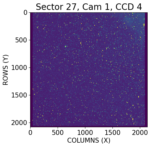
The header information above contains important metadata like the CD matrix elements used for the WCS transformations, exposure time of the observation, size of the image, and so on. Now let’s retrieve the science data from this Primary HDU and plot the sector 27 camera 1 CCD 4 field.
# Retrieve the data and some header metadata for labeling
data = fits.getdata(ffi, 0)
cam, ccd = header['CAMNUM'], header['CCDNUM']

# Plotting
plt.imshow(data, vmin=0, vmax=1000000)

# Labeling
plt.title(f'Sector 27, Cam {cam}, CCD {ccd}', fontsize=20)
plt.xlabel('COLUMNS (X)', fontsize=15)
plt.ylabel('ROWS (Y)', fontsize=15)
plt.tick_params(axis='both', which='major', labelsize=15)

plt.show()
Creating a Cube#
Now that we have retrieved, downloaded, and inspected our TICA FFIs, it’s time to make a cube out of them. To do this, we will call on astrocut’s TicaCubeFactory class which contains all the functionality to stack the TICA FFIs into a cube as efficiently as possible and store all the FFIs’ metadata in a binary table.
tica_cube_maker = TicaCubeFactory()
We will utilize the manifest output from our download_products call in the previous section to feed TicaCubeFactory.make_cube the batch of 5 TICA FFIs for the cube-making process. The verbose argument is set to True by default, which will print updates about the call, but you may change verbose to False if you so choose.
cube = tica_cube_maker.make_cube(manifest['Local Path'])
Using hlsp_tica_tess_ffi_s0027-o1-00116470-cam1-ccd4_tess_v01_img.fits to initialize the image header table.
Cube will be made in 1 blocks of 2079 rows each.
Completed file 0 in 0.0176 sec.
Completed file 1 in 0.013 sec.
Completed file 2 in 0.0128 sec.
Completed file 3 in 0.0124 sec.
Completed file 4 in 0.0125 sec.
Completed block 1 of 1
Total time elapsed: 0.01 min
The cube file is stored in your current working directory with the default name img-cube.fits if none is specified. Let’s inspect the contents of the cube file:
fits.info(cube)
Filename: img-cube.fits
No.    Name      Ver    Type      Cards   Dimensions   Format
  0  PRIMARY       1 PrimaryHDU     182   ()
  1                1 ImageHDU         9   (1, 5, 2136, 2078)   float32
  2                1 BinTableHDU    550   5R x 182C   [J, J, J, J, J, J, J, J, 2A, D, D, D, D, D, D, D, D, D, D, D, D, J, J, J, J, J, J, J, D, J, J, J, J, 16A, D, D, D, D, 9A, 5A, D, 15A, 4A, 4A, D, D, D, D, D, D, D, D, 12A, 12A, D, D, D, D, J, J, D, D, D, D, D, D, D, D, D, D, D, D, D, D, D, D, D, D, D, D, D, D, D, D, D, D, D, D, D, D, D, D, D, D, D, D, D, D, D, D, D, D, D, D, D, D, D, D, D, D, D, D, D, D, D, D, D, D, D, D, D, D, D, D, D, D, D, D, D, D, D, D, D, D, D, D, D, D, D, D, D, D, D, D, D, D, D, D, D, D, D, D, D, D, D, D, D, D, D, D, D, D, D, D, D, D, D, D, D, D, D, D, D, D, D, J, J, J, 16A, 10A, 49A, 64A]
The structure for each cube file is the same for both TICA and SPOC. It consists of:
The Primary HDU, which contains header information derived from the first FFI in the cube stack, as well as WCS information derived from the FFI in the middle of the cube stack.
The Image HDU, which is the cube itself. The dimensions of the cube for this example is
(2, 5, 2136, 2078)and can be explained as follows:The 0th axis represents the science and error “layers”, with the science arrays in index=0 and the error arrays in index=1. Because the TICA pipeline does not propagate errors, the error layer is empty for all the FFIs and should be ignored.
The 1st axis represents the number of FFIs that went into the cube. For this example it is 5. Indexing this will pull out the 2D array of science data for a given FFI.
The 2nd axis represents the number of rows each FFI consists of.
The 3rd axis represents the number of columns each FFI consists of.
The BinTable HDU, which contains the image header information for every FFI that went into the stack in the form of a table. Each column in the table is an image header keyword (for TICA it’s the primary header keyword, since the TICA image lives in the primary HDU), and each row in the column is the corresponding value for that keyword for an FFI.
For more information on the cube file structure, see the cube file format section of the Astrocut documentation.
Before we move onto generating the cutouts, it’s important to note that CubeFactory is distinct from TicaCubeFactory. Both classes are used to generate cubes, but TicaCubeFactory is specifically designed to generate TICA cubes, and CubeFactory is specifically designed to generate SPOC cubes. Any attempt at generating TICA cubes with CubeFactory or vice versa will be unsuccessful. See below for an example:
# This cell will give an error if you uncomment the lines below!

#spoc_cube_maker = CubeFactory()
#spoc_cube_maker.make_cube(manifest['Local Path'])
Creating the Cutouts#
Now that we have our cube we are able to generate cutouts of our region of interest. Unlike in the cube-making process, we have a single class for generating the cutouts from both SPOC or TICA cubes, CutoutFactory. To make the cutouts, we will call upon CutoutFactory’s cube_cut and feed it the cube we just made, the coordinates for the center of our region of interest, which in this case is our object TIC 2527981, the cutout size for our region (in pixels), and lastly, the product type that was used for making our cube.
cutout_maker = CutoutFactory()

cutout_file = cutout_maker.cube_cut(cube, coordinates=coordinates, cutout_size=25, product='TICA')
cutout_file
WARNING: VerifyWarning: Card is too long, comment will be truncated. [astropy.io.fits.card]
'./img_289.097900_-29.337000_25x25_astrocut.fits'
Our cutout file is saved to our current working directory with the default name structured as follows:
img_[RA]_[Dec]_[rows]x[cols]_astrocut.fits
Let’s inspect the HDU list of this file…
fits.info(cutout_file)
Filename: ./img_289.097900_-29.337000_25x25_astrocut.fits
No.    Name      Ver    Type      Cards   Dimensions   Format
  0  PRIMARY     1   PrimaryHDU      57   ()
  1  PIXELS      1   BinTableHDU    277   5R x 11C   [D, J, 625J, 625E, 625E, 625E, 625E, J, E, E, 38A]
  2  APERTURE    1   ImageHDU        82   (25, 25)   int32
The structure for each cutout file is the same for both TICA and SPOC. It consists of:
The Primary HDU, which contains header information derived from the first FFI in the cube stack, as well as WCS information derived from the FFI in the middle of the cube stack.
The BinTable HDU, which is a FITS table that stores the actual cutouts under the
FLUXcolumn, with each row being occupied by a single FFI cutout of the requested size.The Image HDU, which contains the aperture, or field of view, of the cutouts. This image is only useful for the moving targets feature on TESSCut, and should be blank if your target has a set of coordinates assigned to it.
For more information on the cutout file structure, see the target pixel file format section of the Astrocut documentation. For now let’s take a closer look at the Primary HDU header:
cutout_header = fits.getheader(cutout_file, 0)
cutout_header
SIMPLE  =                    T / conforms to FITS standard
BITPIX  =                    8 / array data type
NAXIS   =                    0 / number of array dimensions
EXTEND  =                    T
TICAVER = '0.2.1   '           / tica software version
EQUINOX =               2000.0
INSTRUME= 'TESS Photometer'
TELESCOP= 'TESS    '
CHECKSUM= 'UCDlU9CiUCCiU9Ci'   / HDU checksum updated 2024-02-20T20:59:29
DATASUM = '0       '           / data unit checksum updated 2024-02-20T20:59:29
ORIGIN  = 'STScI/MAST'
DATE    = '2024-02-20'         / FFI cube creation date
SECTOR  =  / Observing sector
EXTNAME = 'PRIMARY '
CREATOR = 'astrocut'           / software used to produce this file
PROCVER = '0.10.1.dev32+g5d0d3e0' / software version
FFI_TYPE= 'TICA    '           / the FFI type used to make the cutouts
RA_OBJ  =             289.0979 / [deg] right ascension
DEC_OBJ =              -29.337 / [deg] declination
TIMEREF =  / barycentric correction applied to times
TASSIGN =  / where time is assigned
TIMESYS = 'TDB     '           / time system is Barycentric Dynamical Time (TDB)
BJDREFI =              2457000 / integer part of BTJD reference date
BJDREFF =                  0.0 / fraction of the day in BTJD reference date
TIMEUNIT= 'd       '           / time unit for TIME, TSTART and TSTOP
EXTVER  = '1       '           / extension version number (not format version)
SIMDATA =                    F / file is based on simulated data
NEXTEND = '2       '           / number of standard extensions
TSTART  =      2036.2780763653 / observation start time in TJD of first FFI
TSTOP   =    2036.312798574792 / observation stop time in TJD of last FFI
CAMERA  =                    1 / Camera number
CCD     =                    4 / CCD chip number
ASTATE  =  / archive state F indicates single orbit processing
CRMITEN =                    T / spacecraft cosmic ray mitigation enabled
CRBLKSZ =  / [exposures] s/c cosmic ray mitigation block siz
FFIINDEX=               116470 / number of FFI cadence interval of first FFI
DATA_REL=  / data release version number
DATE-OBS= '2020-07-05 18:40:25.798' / TSTART as UTC calendar date of first FFI
DATE-END= '2020-07-05 19:30:25.797' / TSTOP as UTC calendar date of last FFI
FILEVER =  / file format version
RADESYS =  / reference frame of celestial coordinates
SCCONFIG=  / spacecraft configuration ID
TIMVERSN=  / OGIP memo number for file format
TELAPSE = 0.034722209491974354 / [d] TSTOP - TSTART
OBJECT  = '' / string version of target id
TCID    =                    0 / unique tess target identifier
PXTABLE =                    0 / pixel table id
PMRA    =                  0.0 / [mas/yr] RA proper motion
PMDEC   =                  0.0 / [mas/yr] Dec proper motion
PMTOTAL =                  0.0 / [mas/yr] total proper motion
TESSMAG =                  0.0 / [mag] TESS magnitude
TEFF    =                  0.0 / [K] Effective temperature
LOGG    =                  0.0 / [cm/s2] log10 surface gravity
MH      =                  0.0 / [log10([M/H])] metallicity
RADIUS  =                  0.0 / [solar radii] stellar radius
TICVER  =                    0 / TICVER
TICID   =  / unique tess target identifier
As mentioned previously, the cutout files will have header information that is inherited from the first FFI and the middle FFI in the cube stack (just like the cube files), so most of these keywords should look familiar. However, there are some new header keywords in the cutout files that are added after processing:
print(cutout_header.cards['FFI_TYPE'])
print(cutout_header.cards['PROCVER'])
FFI_TYPE= 'TICA    '           / the FFI type used to make the cutouts
PROCVER = '0.10.1.dev32+g5d0d3e0' / software version
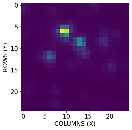
These keywords are intentionally added so that the cutout is formatted like a TESS target pixel file (TPF). Conveniently, this means you can use existing scripts on these cutout files without having to readapt them. Let’s go ahead and plot one of the cutouts in our file:
# Extracting the cutouts science data from the BinTable HDU
cutouts = fits.getdata(cutout_file)['FLUX']

# Plotting an arbitrary cutout from the FLUX column
plt.imshow(cutouts[3])

# Labeling
plt.xlabel('COLUMNS (X)', fontsize=15)
plt.ylabel('ROWS (Y)', fontsize=15)
plt.tick_params(axis='both', which='major', labelsize=15)

plt.show()
Exercise: Generate Cutouts for TIC 2527981 Sector 27 SPOC Products#
Let’s now generate cutouts of our target from the SPOC products of the same observation, and use this as an opportunity to compare the FFI file structure differences between SPOC and TICA.
Perform the same astroquery.mast.Observations query, inspect the FFIs, generate the cube (remember that there are two cube-generating classes, CubeFactory and TicaCubeFactory), and generate the cutouts from the cube, in the cells below.
# Make a query for the correct observation using `astroquery.mast.Observations.query_criteria`

# Retrieve the products corresponding to this observations using `astroquery.mast.Observations.download_products`

# Inspect one of the FFIs with `matplotlib.pyplot`. Compare the HDU List between the SPOC FFI and one of the TICA FFIs
# and note the structural differences.
# Generate a cube with the SPOC FFIs.
# If you've stored the output from the `astroquery.mast.Observations.download_products` call above,
# it's helpful to use the Local Path column as the CubeFactory input.
# Inspect the cube as you wish. Make a note of the cube size and ensure that the dimensions are as you expect.
# Generate the cutouts with the SPOC cube from above.
# Inspect the cutouts as you wish.
Resources#
The following is a list of resources that were referenced throughout the tutorial, as well as some additional references that you may find useful:
astrocut Documentation
astrocut GitHub repository
astroquery.mast Documentation
The TESSCut Service
More information on the TESS mission
More information on the TICA HLSP
Publication on the SPOC Pipeline
Publication on the TICA Quicklook Pipeline
Citations#
If you use any of astroquery’s tools or astrocut for published research, please cite the authors. Follow these links for more information about citing astroquery and astrocut:
About this Notebook#
If you have comments or questions on this notebook, please contact us through the Archive Help Desk e-mail at archive@stsci.edu.
Author(s): Jenny V. Medina
Keyword(s): Tutorial, TESS, TICA, SPOC, astroquery, astrocut, cutouts, ffi, tpf, tesscut
Last Updated: Mar 2023
Top of Page
