Plotting a Catalog over a Kepler Full Frame Image File
This tutorial demonstrates how to access the WCS (World Coordinate System) from a full frame image file and use this data to plot a catalog of objects over the FFI.
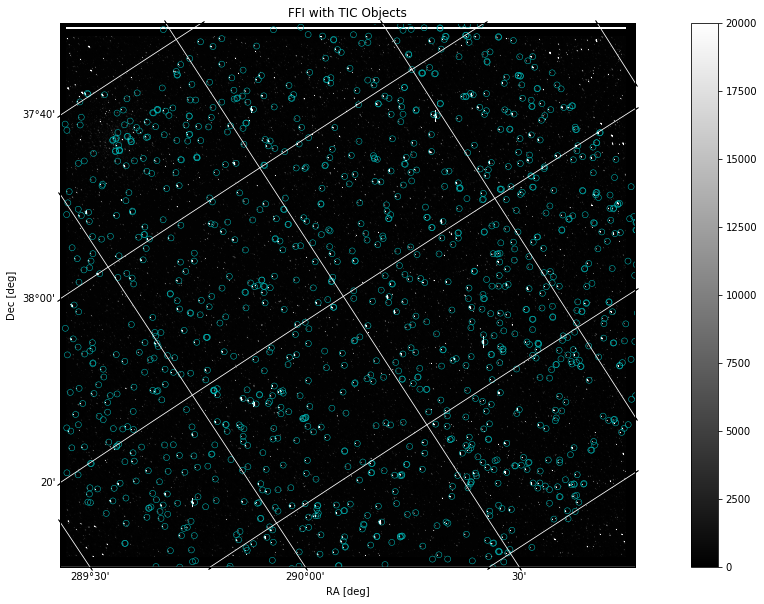
Table of Contents
[Introduction](#intro_ID)
[Imports](#imports_ID)
[Getting the Data](#data_ID)
[File Information](#fileinfo_ID)
[Displaying Image Data](#image_ID)
[Overplotting Objects](#overplot_ID)
[Additional Resources](#resources_ID)
[About this Notebook](#about_ID)
Introduction
Full Frame Image file background: A Full Frame Image (FFI) contains values for every pixel in each of the 84 channels. Standard calibrations, such as flat fields, blacks, and smears have been applied to the calibrated FFIs. These files also contain a World Coordinate System (WCS) that attaches RA and Dec coordinates to pixel x and y values.
Some notes about the file: kplr2009170043915_ffi-cal.fits
The filename contains phrases for identification, where
- kplr = Kepler
- 2009170043915 = year 2009, day 170, time 04:39:15
- ffi-cal = calibrated FFI image
Defining some terms:
- HDU: Header Data Unit; a FITS file is made up of Header or Data units that contain information, data, and metadata relating to the file. The first HDU is called the primary, and anything that follows is considered an extension.
- TIC: TESS Input Catalog; a catalog of luminous sources on the sky to be used by the TESS mission. We will use the TIC in this notebook to query a catalog of objects that we will then plot over an image from Kepler.
- WCS: World Coordinate System; coordinates attached to each pixel of an N-dimensional image of a FITS file. For example, a specified celestial RA and Dec associated with pixel location in the image.
For more information about the Kepler mission and collected data, visit the Kepler archive page. To read more details about light curves and important data terms, look in the Kepler archive manual.
Imports
Let's start by importing some libraries to the environment:
- numpy to handle array functions
- astropy.io fits for accessing fits files
- astropy.wcs WCS to project the World Coordinate System on the plot
- astropy.table Table for creating tidy tables of the data
- matplotlib.pyplot for plotting data
%matplotlib inline
import numpy as np
from astropy.io import fits
from astropy.wcs import WCS
from astropy.table import Table
import matplotlib.pyplot as plt
Getting the Data
Start by importing libraries from Astroquery. For a longer, more detailed description using of Astroquery, please visit this tutorial or read the Astroquery documentation.
from astroquery.mast import Mast
from astroquery.mast import Observations
Next, we need to find the data file. This is similar to searching for the data using the MAST Portal in that we will be using certain keywords to find the file. The object we are looking for is kplr2009170043915, collected by the Kepler spacecraft. We are searching for an FFI file of this object:
kplrObs = Observations.query_criteria(obs_id="kplr2009170043915_84", obs_collection="KeplerFFI")
kplrProds = Observations.get_product_list(kplrObs[0])
yourProd = Observations.filter_products(kplrProds, extension='kplr2009170043915_ffi-cal.fits',
                                        mrp_only=False)
yourProd
Now that we've found the data file, we can download it using the reults shown in the table above:
Observations.download_products(yourProd, mrp_only=False, cache=False)
Reading FITS Extensions
Now that we have the file, we can start working with the data. We will begin by assigning a shorter name to the file to make it easier to use. Then, using the info function from astropy.io.fits, we can see some information about the FITS Header Data Units:
filename = "./mastDownload/KeplerFFI/kplr2009170043915_84/kplr2009170043915_ffi-cal.fits"
fits.info(filename)
- No. 0 (Primary):
This HDU contains meta-data related to the entire file. - No. 1-84 (Image):
Each of the 84 image extensions contains an array that can be plotted as an image. We will plot one in this tutorial along with catalog data.
Let's say we wanted to see more information about the header and extensions than what the fits.info command gave us. For example, we can access information stored in the header of any of the Image extensions (No.1 - 84, MOD.OUT). The following line opens the FITS file, writes the first HDU extension into header1, and then closes the file. Only 24 rows of data are displayed here but you can view them all by adjusting the range:
with fits.open(filename) as hdulist:
    header1 = hdulist[1].header

print(repr(header1[1:25]))
Displaying Image Data
First, let's find the WCS information associated with the FITS file we are using. One way to do this is to access the header and print the rows containing the relevant data (54 - 65). This gives us the reference coordinates (CRVAL1, CRVAL2) that correspond to the reference pixels:
with fits.open(filename) as hdulist:
    header1 = hdulist[1].header

print(repr(header1[54:61]))
Let's pick an image HDU and display its array. We can also choose to print the length of the array to get an idea of the dimensions of the image:
with fits.open(filename) as hdulist:
    imgdata = hdulist[1].data

print(len(imgdata))
print(imgdata)
We can now plot this array as an image:
fig = plt.figure(figsize=(16,8))
plt.imshow(imgdata, cmap=plt.cm.gray)
plt.colorbar()
plt.clim(0,20000)
Now that we've seen the image and the WCS information, we can plot FFI with a WCS projection. To do this, first we will access the file header and assign a WCS object. Then we will plot the image with the projection, and add labels and a grid for usability:
hdu = fits.open(filename)[1]
wcs = WCS(hdu.header)

fig = plt.figure(figsize=(16,8))
ax = plt.subplot(projection=wcs)
im = ax.imshow(hdu.data, cmap=plt.cm.gray, origin='lower', clim=(0,20000))
fig.colorbar(im)

plt.title('FFI with WCS Projection')
ax.set_xlabel('RA [deg]')
ax.set_ylabel('Dec [deg]')
ax.grid(color='white', ls='solid')
Getting the Catalog Data
Now that we have an image, we can use astroquery to retrieve a catalog of objects and overlay it onto the image. First, we will start with importing catalog data from astroquery:
from astroquery.mast import Catalogs
We will query a catalog of objects from TIC (TESS Input Catalog). For more information about TIC, follow this link. Our search will be centered on the same RA and Declination listed in the header of the FFI image and will list objects within a 1 degree radius of that location. It might take a couple seconds longer than usual for this cell to run:
why tic??? explain...
catalogData = Catalogs.query_region("290.4620065226813  38.32946356799192", radius="0.7 deg", catalog="TIC")
dattab = Table(catalogData)
dattab
Let's isolate the RA and Dec columns into a separate table for creating a plot. We will can also filter our results to include only sources brigther than 15 magnitudes in B, which will give us a more managable amount of sources for plotting:
radec = (catalogData['ra','dec','Bmag'])
mask = radec['Bmag'] < 15.0
mag_radec = radec[mask]
print(mag_radec)
We can plot this table to get an idea of what the catalog looks like visually:
fig = plt.figure(figsize=(8,8))
ax = fig.add_subplot(111)
plt.scatter(mag_radec['ra'], mag_radec['dec'], facecolors='none', edgecolors='c', linewidths=0.5)
Overplotting Objects
Now that we have a way to display an FFI file and a catalog of objects, we can put the two pieces of data on the same plot. To do this, we will project the World Coordinate System (WCS) as a grid in units of degrees, minutes, and seconds onto the image. Then, we will create a scatter plot of the catalog, similar to the one above, although here we will transform its coordinate values into ICRS (International Celestial Reference System) to be compatible with the WCS projection:
hdu = fits.open(filename)[1]
wcs = WCS(hdu.header)

fig = plt.figure(figsize=(20,10))
ax = plt.subplot(projection=wcs)
im = ax.imshow(hdu.data, cmap=plt.cm.gray, origin='lower', clim=(0,20000))
fig.colorbar(im)

plt.title('FFI with TIC Catalog Objects')
ax.set_xlabel('RA [deg]')
ax.set_ylabel('Dec [deg]')
ax.grid(color='white', ls='solid')
ax.autoscale(False)

ax.scatter(mag_radec['ra'], mag_radec['dec'],
           facecolors='none', edgecolors='c', linewidths=0.5,
           transform=ax.get_transform('icrs')) # This is needed when projecting onto axes with WCS info
The catalog is displayed here as blue circles that highlight certain objects common in both the Kepler FFI and the TIC search. The image remains in x, y pixel values while the grid is projected in degrees based on the WCS. The projection works off of WCS data in the FFI header to create an accurate grid displaying RA and Dec coordinates that correspond to the original pixel values. The catalog data is transformed into ICRS coordinates in order to work compatibly with the other plotted data.
Aditional Resources
For more information about the MAST archive and details about mission data:
MAST API
Kepler Archive Page (MAST)
Kepler Archive Manual
Exo.MAST website
TESS Archive Page (MAST)
