Simulating WFI Imaging Data with Roman I-Sim#
Nexus Server Information#
IMPORTANT: To run this tutorial, please make sure you are logged in the RRN with a medium server.
Kernel Information and Read-Only Status#
To run this notebook, please select “Roman Research Nexus {VERSION}” kernel at the top right of your window. For example “Roman Research Nexus 2026.1”.
This notebook is read-only. You can run cells and make edits, but you must save changes to a different location. We recommend saving the notebook within your home directory, or to a new folder within your home (e.g. file > save notebook as > my-nbs/nb.ipynb). Note that a directory must exist before you attempt to add a notebook to it.
Introduction#
The purpose of this notebook is to show how to generate simulated Level 1 (L1; uncalibrated ramp cubes) and Level 2 (L2; calibrated rate images) Roman Wide Field Instrument (WFI) Advanced Scientific Data Format (ASDF) files with Roman I-Sim (package name romanisim). Details about the Roman data levels can be found in the Data Levels and Products article in the Roman Documentation System (RDox). Briefly, a L1 file contains a single uncalibrated ramp exposure in units of Data Numbers (DN). L1 files are three-dimensional data cubes, one dimension for time and two dimensions for image coordinates, that are shaped as arrays with (N resultants, 4096 image rows, 4096 image columns). A resultant is a sample up-the-ramp, and represents either a single read of the WFI detectors or multiple reads that have been combined. The L2 WFI data are calibrated images in instrumental units of DN / second. They are two-dimensional arrays shaped as (4088 image rows, 4088 image columns).
In this tutorial we first gather reference data for ancilliary packages as well as import all the packages used in the notebook. Later in the notebook we also offer options to import optimization packages for more advanced use cases.
Reference Data#
The cell below will check to ensure ancillary reference files for the stpsf package are installed. If not, it will download the ancillary reference files and install them under your home directory (i.e., ${HOME}/refdata/).
Local Run Settings#
If you want to run the notebook in your local machine, refer to the information in the local installation instructions before proceeding with the notebook. The instructions provide inportant information about setting up your environment, installing dependnecies, and adding to your working directory scripts to help with the reference data installation.
Depending on which (if any) reference data are missing, this cell may take several minutes to execute.
On the Roman Research Nexus#
If you are working on the Nexus, all the environment variables are defined and the ancillary reference data are pre-installed, so this cell will execute instantly.
import os
import sys
import importlib.util

try:
    import notebook_data_dependencies as ndd
    local = True
except ImportError:
    local = False

# If running locally Get the directory with the script
if not local:
    notebook_dir = os.getcwd()
    shared_path = os.path.abspath(
        os.path.join(notebook_dir, '..', '..', 'shared', 'notebook_data_dependencies.py')
    )

    if os.path.exists(shared_path):
        print(f"Loading notebook_data_dependencies from shared location: {shared_path}")
        spec = importlib.util.spec_from_file_location("notebook_data_dependencies", shared_path)
        ndd = importlib.util.module_from_spec(spec)
        sys.modules['notebook_data_dependencies'] = ndd  # Optional: makes subsequent imports work
        spec.loader.exec_module(ndd)
    else:
        raise FileNotFoundError(f"Local install script not found at {shared_path}")

if not local:
    print("Running local data dependency installation...")
    result = ndd.install_files(packages=['stpsf'])

    # Update environment variables (if necessary) and print reference data paths
    print('Reference data paths set to:')
    for k, v in result.items():
        if not v['pre_installed']:
            os.environ[k] = v['path']
        print(f"\t{k} = {v['path']}")

else:
    print("Running on RNN — data already available, skipping local install.")
Running on RNN — data already available, skipping local install.
Imports#
Libraries used
asdf for opening Roman WFI ASDF files
astroquery.gaia for querying the Gaia catalog
astropy.coordinates for storing celestial coordinates as Python objects
astropy.time for storing time information as Python objects
astropy.table for working with Astropy Table objects
astropy.units for handling and combining units
astropy.visualization for image normalization
copy for making copies of Python objects
galsim for image simulations
importlib for reloading Python modules
matplotlib for displaying images
numpy for array operations
os for file operations
romanisim for image simulations
roman_datamodels for opening Roman WFI ASDF files
s3fs for accessing files in an S3 bucket
stpsf for making PSF profiles at specific detector location.
In the Advanced Use Cases section further below, we include some additional imports:
pysiaf for determining dither positions
dataclasses for creating a class
typing for doing type checking on inputs
dask for parallelization
Note: dask is not installed in the Roman Calibration kernel by default. In the Advanced Use Cases - Parallelized Simulations section, the code cells have been commented out and there is a cell at the beginning of the section that will use pip to install the required packages.
import asdf
from astroquery.gaia import Gaia
from astropy.coordinates import SkyCoord
from astropy.time import Time
from astropy.table import Table, vstack
from astropy import units as u
from astropy.visualization import simple_norm
import copy
import galsim
import importlib
import matplotlib.pyplot as plt
import numpy as np
import os
import roman_datamodels as rdm
from romanisim import gaia, bandpass, catalog, log, wcs, persistence, parameters, ris_make_utils as ris, image as risim
from romanisim.image import inject_sources_into_l2
import s3fs
import stpsf
In preparation for Gaia DR4, the Gaia archive is in evolution. Unfortunately, it may be unstable at times and particular types of queries may time out. Please consider registering for a user account (https://www.cosmos.esa.int/web/gaia-users/register). For questions or advice, please contact the Gaia helpdesk (https://www.cosmos.esa.int/web/gaia/gaia-helpdesk).
2026-06-01 19:44:12 INFO NumExpr defaulting to 8 threads.
Tutorial Data#
In this tutorial, we will create necessary data in memory or retrieve it from a catalog service. A catalog file is also available in the RRN S3 bucket, and can be streamed into memory using astropy.table.Table and the s3fs package instructions in the Data Discovery and Access tutorial. Also see the RRN documentation for more information on the catalog available in the S3 bucket.
Source Catalog Generation#
The romanisim package offers two options for generating source catalogs:
Retrieve the source catalog from Gaia; or
Parametrically generate a catalog of stars and/or galaxies.
First, let’s explore how to create a romanisim-compatible source catalog using Gaia. We will use a combination of astroquery and romanisim to query the Gaia catalog and then write the file in a format compatible with romanisim.
In the example below, we query the Gaia DR3 catalog for sources centered at (RA, Dec) = (270.94, -0.2) degrees within a radius of 1 degree.
Note: The Gaia query may take several minutes to complete.
ra = 270.94   # Right ascension in degrees
dec = -0.2    # Declination in degrees
radius = 1.0  # Search radius in degrees

# Try online query first
try:
    query = f"""
    SELECT *
    FROM gaiadr3.gaia_source
    WHERE 1 = CONTAINS(
        POINT('ICRS', {ra}, {dec}),
        CIRCLE('ICRS', ra, dec, {radius})
    )
    """

    print("Launching async Gaia query...")
    job = Gaia.launch_job_async(query)
    result = job.get_results()
    print(f"Query successful! Retrieved {len(result)} sources.")

except Exception as e:
    print(f"Gaia query failed: {e}")
    print("Trying to load local catalog from directory...")

    local_file = "./catalog_gaia-270p94_m0p2-result.ecsv"

    if os.path.exists(local_file):
        print(f"Loading {local_file} ...")
        result = Table.read(local_file, format='ascii.ecsv')
        print(f"Successfully loaded local catalog with {len(result)} sources.")
    else:
        print(f"Local file '{local_file}' not found in current directory.")
        print("Current directory contents:")
        print(os.listdir('.'))
        result = None

# If you got results (online or local)
if result is not None:
    #print(result.info)
    # show first few rows
    print(result[:5])
else:
    print("No catalog available.")
Launching async Gaia query...
2026-06-01 19:52:41 INFO Query finished.
INFO: Query finished. [astroquery.utils.tap.core]
Query successful! Retrieved 389468 sources.
    solution_id             designation          ... libname_gspphot
                                                 ...
------------------- ---------------------------- ... ---------------
1636148068921376768 Gaia DR3 4179306919097309440 ...           MARCS
1636148068921376768 Gaia DR3 4179306919097335680 ...
1636148068921376768 Gaia DR3 4179307022176616576 ...
1636148068921376768 Gaia DR3 4179307026477535360 ...
1636148068921376768 Gaia DR3 4179307232632289408 ...
Once we have the result from the Gaia query, we can transform it into a format compatible with Roman I-Sim:
# Filter the Gaia results for stars and exclude bright stars
result = result[result['classprob_dsc_combmod_star'] >= 0.7]
result = result[result['phot_g_mean_mag'] > 16.5]

# Set the observation time
obs_time = '2026-10-31T00:00:00'

# Make the Roman I-Sim formatted catalog
gaia_catalog = gaia.gaia2romanisimcat(result, Time(obs_time), fluxfields=set(bandpass.galsim2roman_bandpass.values()))
We have excluded very bright stars (Gaia g-band > 16.5 mag in this example) because Roman I-Sim uses a maximum size of the simulated point spread function (PSF) in pixels that can result in the appearance of box-shaped boundaries around bright sources. This will be fixed in a future update.
When using a real catalog like Gaia, it is essential to remove any entries with missing information. This can be achieved with the code in the cell below:
# Reject anything with missing fluxes or positions
names = [f for f in gaia_catalog.dtype.names if f[0] == 'F']
names += ['ra', 'dec']

bad = np.zeros(len(gaia_catalog), dtype='bool')
for b in names:
    bad = ~np.isfinite(gaia_catalog[b])
    if hasattr(gaia_catalog[b], 'mask'):
        bad = gaia_catalog[b].mask
    gaia_catalog = gaia_catalog[~bad]
Now that we have a catalog, let’s take a look at it. The catalog in memory is an astropy.table.Table object with over 1e5 rows:
gaia_catalog
| ra | dec | type | n | half_light_radius | pa | ba | F158 | F213 | F106 | F087 | F146 | F184 | F129 | F062 |
|---|---|---|---|---|---|---|---|---|---|---|---|---|---|---|
| float64 | float64 | str3 | int64 | int64 | int64 | int64 | float64 | float64 | float64 | float64 | float64 | float64 | float64 | float64 |
| 269.99556833474514 | -0.5153686985148954 | PSF | -1 | -1 | -1 | -1 | 4.453445444244283e-08 | 4.453445444244283e-08 | 4.453445444244283e-08 | 4.453445444244283e-08 | 4.453445444244283e-08 | 4.453445444244283e-08 | 4.453445444244283e-08 | 4.453445444244283e-08 |
| 269.99857867515965 | -0.5091925233797133 | PSF | -1 | -1 | -1 | -1 | 2.5630046236381587e-08 | 2.5630046236381587e-08 | 2.5630046236381587e-08 | 2.5630046236381587e-08 | 2.5630046236381587e-08 | 2.5630046236381587e-08 | 2.5630046236381587e-08 | 2.5630046236381587e-08 |
| 269.99369961265984 | -0.4947976090170517 | PSF | -1 | -1 | -1 | -1 | 1.4801210707489509e-08 | 1.4801210707489509e-08 | 1.4801210707489509e-08 | 1.4801210707489509e-08 | 1.4801210707489509e-08 | 1.4801210707489509e-08 | 1.4801210707489509e-08 | 1.4801210707489509e-08 |
| 269.9974539783147 | -0.48975487534172074 | PSF | -1 | -1 | -1 | -1 | 1.631640058361595e-08 | 1.631640058361595e-08 | 1.631640058361595e-08 | 1.631640058361595e-08 | 1.631640058361595e-08 | 1.631640058361595e-08 | 1.631640058361595e-08 | 1.631640058361595e-08 |
| 269.9916566781788 | -0.49074850696407196 | PSF | -1 | -1 | -1 | -1 | 1.1705312862630533e-08 | 1.1705312862630533e-08 | 1.1705312862630533e-08 | 1.1705312862630533e-08 | 1.1705312862630533e-08 | 1.1705312862630533e-08 | 1.1705312862630533e-08 | 1.1705312862630533e-08 |
| 269.99891226347086 | -0.4771143072821228 | PSF | -1 | -1 | -1 | -1 | 5.875144528123327e-08 | 5.875144528123327e-08 | 5.875144528123327e-08 | 5.875144528123327e-08 | 5.875144528123327e-08 | 5.875144528123327e-08 | 5.875144528123327e-08 | 5.875144528123327e-08 |
| 269.99498980449675 | -0.4584007154938247 | PSF | -1 | -1 | -1 | -1 | 8.52024268951623e-09 | 8.52024268951623e-09 | 8.52024268951623e-09 | 8.52024268951623e-09 | 8.52024268951623e-09 | 8.52024268951623e-09 | 8.52024268951623e-09 | 8.52024268951623e-09 |
| 269.9750938243964 | -0.45516614685890483 | PSF | -1 | -1 | -1 | -1 | 3.5485889395606015e-08 | 3.5485889395606015e-08 | 3.5485889395606015e-08 | 3.5485889395606015e-08 | 3.5485889395606015e-08 | 3.5485889395606015e-08 | 3.5485889395606015e-08 | 3.5485889395606015e-08 |
| 269.9983871538959 | -0.44846896942283615 | PSF | -1 | -1 | -1 | -1 | 1.1138740597782383e-08 | 1.1138740597782383e-08 | 1.1138740597782383e-08 | 1.1138740597782383e-08 | 1.1138740597782383e-08 | 1.1138740597782383e-08 | 1.1138740597782383e-08 | 1.1138740597782383e-08 |
| ... | ... | ... | ... | ... | ... | ... | ... | ... | ... | ... | ... | ... | ... | ... |
| 270.9167043261976 | 0.782678973589976 | PSF | -1 | -1 | -1 | -1 | 6.80578323724805e-09 | 6.80578323724805e-09 | 6.80578323724805e-09 | 6.80578323724805e-09 | 6.80578323724805e-09 | 6.80578323724805e-09 | 6.80578323724805e-09 | 6.80578323724805e-09 |
| 270.88979840625507 | 0.7747874618110461 | PSF | -1 | -1 | -1 | -1 | 8.128916337031148e-09 | 8.128916337031148e-09 | 8.128916337031148e-09 | 8.128916337031148e-09 | 8.128916337031148e-09 | 8.128916337031148e-09 | 8.128916337031148e-09 | 8.128916337031148e-09 |
| 270.900239321006 | 0.7898552447805102 | PSF | -1 | -1 | -1 | -1 | 5.636012982912401e-09 | 5.636012982912401e-09 | 5.636012982912401e-09 | 5.636012982912401e-09 | 5.636012982912401e-09 | 5.636012982912401e-09 | 5.636012982912401e-09 | 5.636012982912401e-09 |
| 270.8957011704554 | 0.7934091590811507 | PSF | -1 | -1 | -1 | -1 | 1.3192357696256221e-07 | 1.3192357696256221e-07 | 1.3192357696256221e-07 | 1.3192357696256221e-07 | 1.3192357696256221e-07 | 1.3192357696256221e-07 | 1.3192357696256221e-07 | 1.3192357696256221e-07 |
| 270.8602731241303 | 0.7722406411775035 | PSF | -1 | -1 | -1 | -1 | 1.6255889638724214e-08 | 1.6255889638724214e-08 | 1.6255889638724214e-08 | 1.6255889638724214e-08 | 1.6255889638724214e-08 | 1.6255889638724214e-08 | 1.6255889638724214e-08 | 1.6255889638724214e-08 |
| 270.8511915751305 | 0.7919003527379259 | PSF | -1 | -1 | -1 | -1 | 2.7309828302333074e-08 | 2.7309828302333074e-08 | 2.7309828302333074e-08 | 2.7309828302333074e-08 | 2.7309828302333074e-08 | 2.7309828302333074e-08 | 2.7309828302333074e-08 | 2.7309828302333074e-08 |
| 270.85445136932003 | 0.7942069013589257 | PSF | -1 | -1 | -1 | -1 | 6.86069002623e-09 | 6.86069002623e-09 | 6.86069002623e-09 | 6.86069002623e-09 | 6.86069002623e-09 | 6.86069002623e-09 | 6.86069002623e-09 | 6.86069002623e-09 |
| 270.8817855132803 | 0.7874186642257874 | PSF | -1 | -1 | -1 | -1 | 1.7352999019231416e-08 | 1.7352999019231416e-08 | 1.7352999019231416e-08 | 1.7352999019231416e-08 | 1.7352999019231416e-08 | 1.7352999019231416e-08 | 1.7352999019231416e-08 | 1.7352999019231416e-08 |
| 270.87169387058583 | 0.7921955153681981 | PSF | -1 | -1 | -1 | -1 | 2.4905581828141572e-08 | 2.4905581828141572e-08 | 2.4905581828141572e-08 | 2.4905581828141572e-08 | 2.4905581828141572e-08 | 2.4905581828141572e-08 | 2.4905581828141572e-08 | 2.4905581828141572e-08 |
| 270.8958710175795 | 0.7987174311757861 | PSF | -1 | -1 | -1 | -1 | 5.900278312902457e-08 | 5.900278312902457e-08 | 5.900278312902457e-08 | 5.900278312902457e-08 | 5.900278312902457e-08 | 5.900278312902457e-08 | 5.900278312902457e-08 | 5.900278312902457e-08 |
Alternatively, we can generate a completely synthetic catalog of stars and galaxies using tools in Roman I-Sim (see parameters in the cell below). In this tutorial, we will simulate a galaxy catalog and merge it with the Gaia star catalog. This approach addresses the limitation of Gaia’s catalog, which includes only relatively bright sources, by adding galaxies. At the same time, real Gaia point sources are necessary for the Roman calibration pipeline to match images to Gaia astrometry.
Note that we can additionally simulate a star catalog if desired. This may be useful for including stars fainter than the Gaia magnitude limit, or when the Gaia astrometric step in RomanCal is not required.
Note that in the cell below, we have commented out the last line, which would save the catalog to disk as an Enhanced Character-Separated Values (ECSV) file. We do not need the catalog to be saved on disk for this tutorial, but you may optionally uncomment the line to save the file if you wish. The same file is available in the S3 bucket for any other tutorials that may need it. Having a saved version of the catalog removes the need to re-run the Gaia query above if you need to start over, but you will need to add code to read the catalog file below.
# Galaxy catalog parameters

ra = 270.94  # Right ascension of the catalog center in degrees
dec = -0.2  # Declination of the catalog center in degrees
radius = 1.0  # Radius of the catalog in degrees
n_gal = 30_000  # Number of galaxies
faint_mag = 22  # Faint magnitude limit of simulated sources
hlight_radius = 0.3  # Half-light radius at the faint magnitude limit in units of arcseconds
optical_element = 'F062 F087 F106 F129 F146 F158 F184 F213'.split()  # List of optical elements to simulate
seed = 4642  # Random number seed for reproducibility

# Create galaxy catalog
galaxy_cat = catalog.make_galaxies(SkyCoord(ra, dec, unit='deg'), n_gal, radius=radius, index=0.4, faintmag=faint_mag,
                                   hlr_at_faintmag=hlight_radius, bandpasses=optical_element, rng=None, seed=seed)

# Merge the galaxy and Gaia catalogs
full_catalog = vstack([galaxy_cat, gaia_catalog])

# To save the catalog to disk, uncomment the following line
#full_catalog.write('full_catalog.ecsv', format='ascii.ecsv', overwrite=True)
The following cell is commented out, but if uncommented will create a simulated star catalog.
#n_star = 30_000  # Number of stars

#star_cat = catalog.make_stars(SkyCoord(ra, dec, unit='deg'), n_star, radius=radius, index=5/3., faintmag=faint_mag,
#                              truncation_radius=None, bandpasses=optical_element, rng=None, seed=seed)
As before, we have commented out the line that will write this to disk, and instead have kept it in memory. Below, let’s print out the catalog and take a look:
full_catalog
| ra | dec | type | n | half_light_radius | pa | ba | F062 | F087 | F106 | F129 | F146 | F158 | F184 | F213 |
|---|---|---|---|---|---|---|---|---|---|---|---|---|---|---|
| float64 | float64 | str3 | float64 | float64 | float64 | float64 | float64 | float64 | float64 | float64 | float64 | float64 | float64 | float64 |
| 271.6295510520961 | -0.03965028067096237 | SER | 3.516215236599453 | 0.8056893348693848 | 252.7303924560547 | 0.7235707640647888 | 3.6905281053378758e-09 | 1.1479291295302119e-08 | 1.2472877841673835e-08 | 6.86679868522333e-09 | 1.4913801305027619e-09 | 1.0117606308313043e-08 | 4.943988773931096e-09 | 2.402744225804554e-09 |
| 270.7539155586658 | -1.175434326974954 | SER | 1.0399398592419549 | 0.946480393409729 | 336.08306884765625 | 0.4800519347190857 | 3.1115434673267828e-09 | 5.331648900153141e-09 | 9.049362148516593e-09 | 6.6658691899590394e-09 | 2.0099595321454444e-09 | 1.5802696040623232e-08 | 1.0280717610555712e-08 | 1.096286439405958e-08 |
| 270.8648924331985 | 0.5861049874846664 | SER | 2.8206730415136585 | 1.3277175426483154 | 73.26484680175781 | 0.6938181519508362 | 1.3153379718744418e-08 | 6.075517422488019e-09 | 3.1850986292880634e-09 | 7.20732051817663e-09 | 6.512435035688213e-09 | 6.66888944067523e-09 | 4.776757656088648e-09 | 6.596417634341378e-09 |
| 270.70544440611565 | -0.1905627389524337 | SER | 1.2080757918109357 | 0.573934018611908 | 273.72601318359375 | 0.5772462487220764 | 3.2391787030405794e-09 | 1.9316861443741118e-09 | 3.5669256437387276e-09 | 1.699146068290247e-08 | 9.461913919039944e-09 | 7.503919152718197e-10 | 4.7414845383286774e-09 | 5.4636619672976394e-09 |
| 271.0763272819082 | 0.28776831750222365 | SER | 2.7301807784747587 | 5.05323600769043 | 236.8221435546875 | 0.907397985458374 | 7.582467986821939e-08 | 7.082852704343168e-08 | 3.547680762494565e-07 | 2.0032227610045084e-07 | 2.793574651605013e-07 | 2.3345998556578706e-07 | 3.1447200399270514e-07 | 1.8613071972595208e-07 |
| 271.1748280956513 | 0.707003102302135 | SER | 3.1848109641065934 | 0.10060989856719971 | 126.41947937011719 | 0.7899426817893982 | 1.5315970713913885e-09 | 8.170578102983939e-10 | 1.1321914517026244e-09 | 5.698110872032203e-09 | 3.009007709664502e-09 | 2.8135679897012267e-10 | 2.320242442621634e-09 | 2.7085311771202214e-09 |
| 270.2732744737068 | -0.5242855117710061 | SER | 2.170910622844513 | 0.7404346466064453 | 333.9393005371094 | 0.5321943163871765 | 4.550629206789836e-09 | 6.8587584500789944e-09 | 3.520021607528179e-08 | 6.720015477412744e-08 | 1.7618161507471086e-07 | 5.838797179080757e-08 | 3.523029690200019e-08 | 2.141273469646876e-08 |
| 271.4612060810417 | 0.48981218301356017 | SER | 3.9307805517506704 | 0.30752477049827576 | 114.4226303100586 | 0.26505595445632935 | 6.278863207143104e-09 | 6.867115764919163e-10 | 1.5396568464609572e-09 | 1.934612026133209e-09 | 4.098307027078363e-09 | 1.5311047985022697e-09 | 4.907185768843192e-09 | 1.902641377782288e-09 |
| 270.5213999343187 | 0.3768383558530194 | SER | 1.1385050100070848 | 0.8638880848884583 | 180.25221252441406 | 0.6406149864196777 | 2.1948302730834257e-07 | 1.7533350771259393e-08 | 2.676470600704306e-08 | 6.562089538419968e-08 | 2.8127658424637048e-08 | 1.7247877792669897e-08 | 1.6523750900887535e-07 | 2.2672709931725876e-08 |
| ... | ... | ... | ... | ... | ... | ... | ... | ... | ... | ... | ... | ... | ... | ... |
| 270.9167043261976 | 0.782678973589976 | PSF | -1.0 | -1.0 | -1.0 | -1.0 | 6.80578323724805e-09 | 6.80578323724805e-09 | 6.80578323724805e-09 | 6.80578323724805e-09 | 6.80578323724805e-09 | 6.80578323724805e-09 | 6.80578323724805e-09 | 6.80578323724805e-09 |
| 270.88979840625507 | 0.7747874618110461 | PSF | -1.0 | -1.0 | -1.0 | -1.0 | 8.128916337031148e-09 | 8.128916337031148e-09 | 8.128916337031148e-09 | 8.128916337031148e-09 | 8.128916337031148e-09 | 8.128916337031148e-09 | 8.128916337031148e-09 | 8.128916337031148e-09 |
| 270.900239321006 | 0.7898552447805102 | PSF | -1.0 | -1.0 | -1.0 | -1.0 | 5.636012982912401e-09 | 5.636012982912401e-09 | 5.636012982912401e-09 | 5.636012982912401e-09 | 5.636012982912401e-09 | 5.636012982912401e-09 | 5.636012982912401e-09 | 5.636012982912401e-09 |
| 270.8957011704554 | 0.7934091590811507 | PSF | -1.0 | -1.0 | -1.0 | -1.0 | 1.3192357696256221e-07 | 1.3192357696256221e-07 | 1.3192357696256221e-07 | 1.3192357696256221e-07 | 1.3192357696256221e-07 | 1.3192357696256221e-07 | 1.3192357696256221e-07 | 1.3192357696256221e-07 |
| 270.8602731241303 | 0.7722406411775035 | PSF | -1.0 | -1.0 | -1.0 | -1.0 | 1.6255889638724214e-08 | 1.6255889638724214e-08 | 1.6255889638724214e-08 | 1.6255889638724214e-08 | 1.6255889638724214e-08 | 1.6255889638724214e-08 | 1.6255889638724214e-08 | 1.6255889638724214e-08 |
| 270.8511915751305 | 0.7919003527379259 | PSF | -1.0 | -1.0 | -1.0 | -1.0 | 2.7309828302333074e-08 | 2.7309828302333074e-08 | 2.7309828302333074e-08 | 2.7309828302333074e-08 | 2.7309828302333074e-08 | 2.7309828302333074e-08 | 2.7309828302333074e-08 | 2.7309828302333074e-08 |
| 270.85445136932003 | 0.7942069013589257 | PSF | -1.0 | -1.0 | -1.0 | -1.0 | 6.86069002623e-09 | 6.86069002623e-09 | 6.86069002623e-09 | 6.86069002623e-09 | 6.86069002623e-09 | 6.86069002623e-09 | 6.86069002623e-09 | 6.86069002623e-09 |
| 270.8817855132803 | 0.7874186642257874 | PSF | -1.0 | -1.0 | -1.0 | -1.0 | 1.7352999019231416e-08 | 1.7352999019231416e-08 | 1.7352999019231416e-08 | 1.7352999019231416e-08 | 1.7352999019231416e-08 | 1.7352999019231416e-08 | 1.7352999019231416e-08 | 1.7352999019231416e-08 |
| 270.87169387058583 | 0.7921955153681981 | PSF | -1.0 | -1.0 | -1.0 | -1.0 | 2.4905581828141572e-08 | 2.4905581828141572e-08 | 2.4905581828141572e-08 | 2.4905581828141572e-08 | 2.4905581828141572e-08 | 2.4905581828141572e-08 | 2.4905581828141572e-08 | 2.4905581828141572e-08 |
| 270.8958710175795 | 0.7987174311757861 | PSF | -1.0 | -1.0 | -1.0 | -1.0 | 5.900278312902457e-08 | 5.900278312902457e-08 | 5.900278312902457e-08 | 5.900278312902457e-08 | 5.900278312902457e-08 | 5.900278312902457e-08 | 5.900278312902457e-08 | 5.900278312902457e-08 |
We can see galaxies at the top of the stacked catalog (notice type == “SER” for Sersic and values of n (the Sersic index) are not -1, while stars have type == PSF).
If using an existing catalog, here we provide with the command to read it
# Read saved catalog
#full_catalog = Table.read('full_catalog.ecsv')
Image Simulation#
Here we show how to run the actual simulation using Roman I-Sim. The method for running the simulation for both L1 and L2 data is the same, so we will show an example for L2, and give instructions of how to modify this for L1.
In our example, we are simulating only a single image, so we have set the persistance to the default. Future updates may include how to simulate persistance from multiple exposures.
Notes:
Roman I-Sim allows the user to either use reference files from CRDS or to use no reference files. The latter is not recommended.
Each detector is simulated separately. Below, in the Advanced Use Cases - Parallelized Simulations section, we include instructions on how to parallelize the simulations using Dask.
Currently, the simulator does not include the effect of 1/f noise.
Multi-accumulation (MA) tables control the total exposure time and sampling up-the-ramp. For more information, see the MA table article in the Roman APT Users Guide.
In this case, we will create an observation using the detector WFI01 and the F106 optical element. The observation is simulated to occur at UTC time 2026-10-31T00:00:00 and an exposure time of approximately 60 seconds.
Note: It will take several minutes to download the appropriate calibration reference files the first time this cell is run. Any changes to the settings below may require downloading additional files, which could increase the run time.
Note To avoid writing files unnecessarily and reduce I/O overdead, the simulated file is not saved to disk. This provides batch processing flesibility, where you inspect/modify your file before saving. For simplicity, the command to save your file is also provided.
# WFI data level to simulate...1 or 2
level = 2

# Other important parameters
obs_date = '2026-10-31T00:00:00'  # Datetime of the simulated exposure
optical_element = 'F106'  # Optical element to simulate
ma_table_number = 1018  # Multi-accumulation (MA) table number (see RDox for more information)
seed = 7  # Galsim random number generator seed for reproducibility
sca = 1  # Change this number to simulate different WFI detectors 1 - 18

# If using CRDS, set reference_data to None
for k in parameters.reference_data:
    parameters.reference_data[k] = None

# Set Galsim RNG object
rng = galsim.UniformDeviate(seed)

# Set default persistance information
persist = persistence.Persistence()

# Set metadata for use in Roman I-Sim.
metadata = ris.set_metadata(date=obs_date, bandpass=optical_element,
                            sca=sca, ma_table_number=ma_table_number, usecrds=True)

# Update the WCS info
wcs.fill_in_parameters(metadata, SkyCoord(ra, dec, unit='deg', frame='icrs'),
                       boresight=False, pa_aper=0.0)

# Run the simulation using metadata valueswithout saving any files
im, extras = risim.simulate(metadata, full_catalog, usecrds=True,
                            psftype='stpsf', level=level,
                            persistence=None, rng=rng
                            )
2026-06-01 19:52:45 WARNING 7412 points with problematic saturation / inverse linearity values!
2026-06-01 19:52:45 INFO Simulating filter F106...
2026-06-01 19:52:45 INFO Creating PSF using stpsf
2026-06-01 19:52:45 INFO Using pupil mask 'F062' and detector 'WFI01'.
2026-06-01 19:52:45 INFO Using pupil mask 'F062' and detector 'WFI01'.
2026-06-01 19:52:46 INFO Using pupil mask 'F106' and detector 'WFI01'.
2026-06-01 19:52:46 INFO No source spectrum supplied, therefore defaulting to 5700 K blackbody
2026-06-01 19:52:46 INFO Computing wavelength weights using synthetic photometry for F106...
2026-06-01 19:52:46 INFO Using pupil mask 'F106' and detector 'WFI01'.
2026-06-01 19:52:46 INFO PSF calc using fov_arcsec = 5.000000, oversample = 4, number of wavelengths = 10
2026-06-01 19:52:46 INFO Creating optical system model:
2026-06-01 19:52:46 INFO Initialized OpticalSystem: Roman+WFI
2026-06-01 19:52:46 INFO Roman Entrance Pupil: Loaded amplitude transmission from /home/runner/refdata/stpsf-data/WFI/pupils/RST_WIM_Filter_F106_WFI01.fits.gz
2026-06-01 19:52:46 INFO Roman Entrance Pupil: Loaded OPD from /home/runner/refdata/stpsf-data/upscaled_HST_OPD.fits
2026-06-01 19:52:46 INFO Added pupil plane: Roman Entrance Pupil
2026-06-01 19:52:46 INFO Added coordinate inversion plane: OTE exit pupil
2026-06-01 19:52:46 INFO Added pupil plane: Field Dependent Aberration (WFI01)
2026-06-01 19:52:46 INFO Added detector with pixelscale=0.1078577405 and oversampling=4: WFI detector
2026-06-01 19:52:46 INFO Calculating PSF with 10 wavelengths
2026-06-01 19:52:46 INFO Propagating wavelength = 9.4555e-07 m
2026-06-01 19:52:51 INFO Propagating wavelength = 9.7265e-07 m
2026-06-01 19:52:52 INFO Propagating wavelength = 9.9975e-07 m
2026-06-01 19:52:52 INFO Propagating wavelength = 1.02685e-06 m
2026-06-01 19:52:52 INFO Propagating wavelength = 1.05395e-06 m
2026-06-01 19:52:53 INFO Propagating wavelength = 1.08105e-06 m
2026-06-01 19:52:53 INFO Propagating wavelength = 1.10815e-06 m
2026-06-01 19:52:53 INFO Propagating wavelength = 1.13525e-06 m
2026-06-01 19:52:54 INFO Propagating wavelength = 1.16235e-06 m
2026-06-01 19:52:54 INFO Propagating wavelength = 1.18945e-06 m
2026-06-01 19:52:54 INFO Calculation completed in 8.467 s
2026-06-01 19:52:54 INFO PSF Calculation completed.
2026-06-01 19:52:54 INFO Calculating jitter using gaussian
2026-06-01 19:52:54 INFO Jitter: Convolving with Gaussian with sigma=0.012 arcsec
2026-06-01 19:52:54 INFO resulting image peak drops to 0.946 of its previous value
2026-06-01 19:52:54 INFO Detector charge diffusion not applied because charge_diffusion_sigma option is 0
2026-06-01 19:52:54 INFO Adding extension with image downsampled to detector pixel scale.
2026-06-01 19:52:54 INFO Downsampling to detector pixel scale, by 4
2026-06-01 19:52:54 INFO Downsampling to detector pixel scale, by 4
2026-06-01 19:52:54 INFO Creating PSF using stpsf
2026-06-01 19:52:55 INFO Using pupil mask 'F062' and detector 'WFI01'.
2026-06-01 19:52:55 INFO Using pupil mask 'F062' and detector 'WFI01'.
2026-06-01 19:52:55 INFO Using pupil mask 'F106' and detector 'WFI01'.
2026-06-01 19:52:55 INFO No source spectrum supplied, therefore defaulting to 5700 K blackbody
2026-06-01 19:52:55 INFO Computing wavelength weights using synthetic photometry for F106...
2026-06-01 19:52:55 INFO Using pupil mask 'F106' and detector 'WFI01'.
2026-06-01 19:52:55 INFO PSF calc using fov_arcsec = 5.000000, oversample = 4, number of wavelengths = 10
2026-06-01 19:52:55 INFO Creating optical system model:
2026-06-01 19:52:55 INFO Initialized OpticalSystem: Roman+WFI
2026-06-01 19:52:55 INFO Roman Entrance Pupil: Loaded amplitude transmission from /home/runner/refdata/stpsf-data/WFI/pupils/RST_WIM_Filter_F106_WFI01.fits.gz
2026-06-01 19:52:55 INFO Roman Entrance Pupil: Loaded OPD from /home/runner/refdata/stpsf-data/upscaled_HST_OPD.fits
2026-06-01 19:52:55 INFO Added pupil plane: Roman Entrance Pupil
2026-06-01 19:52:55 INFO Added coordinate inversion plane: OTE exit pupil
2026-06-01 19:52:55 INFO Added pupil plane: Field Dependent Aberration (WFI01)
2026-06-01 19:52:55 INFO Added detector with pixelscale=0.1078577405 and oversampling=4: WFI detector
2026-06-01 19:52:55 INFO Calculating PSF with 10 wavelengths
2026-06-01 19:52:55 INFO Propagating wavelength = 9.4555e-07 m
2026-06-01 19:52:55 INFO Propagating wavelength = 9.7265e-07 m
2026-06-01 19:52:56 INFO Propagating wavelength = 9.9975e-07 m
2026-06-01 19:52:56 INFO Propagating wavelength = 1.02685e-06 m
2026-06-01 19:52:56 INFO Propagating wavelength = 1.05395e-06 m
2026-06-01 19:52:57 INFO Propagating wavelength = 1.08105e-06 m
2026-06-01 19:52:57 INFO Propagating wavelength = 1.10815e-06 m
2026-06-01 19:52:57 INFO Propagating wavelength = 1.13525e-06 m
2026-06-01 19:52:58 INFO Propagating wavelength = 1.16235e-06 m
2026-06-01 19:52:58 INFO Propagating wavelength = 1.18945e-06 m
2026-06-01 19:52:58 INFO Calculation completed in 3.242 s
2026-06-01 19:52:58 INFO PSF Calculation completed.
2026-06-01 19:52:58 INFO Calculating jitter using gaussian
2026-06-01 19:52:58 INFO Jitter: Convolving with Gaussian with sigma=0.012 arcsec
2026-06-01 19:52:58 INFO resulting image peak drops to 0.946 of its previous value
2026-06-01 19:52:58 INFO Detector charge diffusion not applied because charge_diffusion_sigma option is 0
2026-06-01 19:52:58 INFO Adding extension with image downsampled to detector pixel scale.
2026-06-01 19:52:58 INFO Downsampling to detector pixel scale, by 4
2026-06-01 19:52:58 INFO Downsampling to detector pixel scale, by 4
2026-06-01 19:52:58 INFO Creating PSF using stpsf
2026-06-01 19:52:58 INFO Using pupil mask 'F062' and detector 'WFI01'.
2026-06-01 19:52:58 INFO Using pupil mask 'F062' and detector 'WFI01'.
2026-06-01 19:52:59 INFO Using pupil mask 'F106' and detector 'WFI01'.
2026-06-01 19:52:59 INFO No source spectrum supplied, therefore defaulting to 5700 K blackbody
2026-06-01 19:52:59 INFO Computing wavelength weights using synthetic photometry for F106...
2026-06-01 19:52:59 INFO Using pupil mask 'F106' and detector 'WFI01'.
2026-06-01 19:52:59 INFO PSF calc using fov_arcsec = 5.000000, oversample = 4, number of wavelengths = 10
2026-06-01 19:52:59 INFO Creating optical system model:
2026-06-01 19:52:59 INFO Initialized OpticalSystem: Roman+WFI
2026-06-01 19:52:59 INFO Roman Entrance Pupil: Loaded amplitude transmission from /home/runner/refdata/stpsf-data/WFI/pupils/RST_WIM_Filter_F106_WFI01.fits.gz
2026-06-01 19:52:59 INFO Roman Entrance Pupil: Loaded OPD from /home/runner/refdata/stpsf-data/upscaled_HST_OPD.fits
2026-06-01 19:52:59 INFO Added pupil plane: Roman Entrance Pupil
2026-06-01 19:52:59 INFO Added coordinate inversion plane: OTE exit pupil
2026-06-01 19:52:59 INFO Added pupil plane: Field Dependent Aberration (WFI01)
2026-06-01 19:52:59 INFO Added detector with pixelscale=0.1078577405 and oversampling=4: WFI detector
2026-06-01 19:52:59 INFO Calculating PSF with 10 wavelengths
2026-06-01 19:52:59 INFO Propagating wavelength = 9.4555e-07 m
2026-06-01 19:52:59 INFO Propagating wavelength = 9.7265e-07 m
2026-06-01 19:53:00 INFO Propagating wavelength = 9.9975e-07 m
2026-06-01 19:53:00 INFO Propagating wavelength = 1.02685e-06 m
2026-06-01 19:53:00 INFO Propagating wavelength = 1.05395e-06 m
2026-06-01 19:53:01 INFO Propagating wavelength = 1.08105e-06 m
2026-06-01 19:53:01 INFO Propagating wavelength = 1.10815e-06 m
2026-06-01 19:53:01 INFO Propagating wavelength = 1.13525e-06 m
2026-06-01 19:53:01 INFO Propagating wavelength = 1.16235e-06 m
2026-06-01 19:53:02 INFO Propagating wavelength = 1.18945e-06 m
2026-06-01 19:53:02 INFO Calculation completed in 3.222 s
2026-06-01 19:53:02 INFO PSF Calculation completed.
2026-06-01 19:53:02 INFO Calculating jitter using gaussian
2026-06-01 19:53:02 INFO Jitter: Convolving with Gaussian with sigma=0.012 arcsec
2026-06-01 19:53:02 INFO resulting image peak drops to 0.946 of its previous value
2026-06-01 19:53:02 INFO Detector charge diffusion not applied because charge_diffusion_sigma option is 0
2026-06-01 19:53:02 INFO Adding extension with image downsampled to detector pixel scale.
2026-06-01 19:53:02 INFO Downsampling to detector pixel scale, by 4
2026-06-01 19:53:02 INFO Downsampling to detector pixel scale, by 4
2026-06-01 19:53:02 INFO Creating PSF using stpsf
2026-06-01 19:53:02 INFO Using pupil mask 'F062' and detector 'WFI01'.
2026-06-01 19:53:02 INFO Using pupil mask 'F062' and detector 'WFI01'.
2026-06-01 19:53:02 INFO Using pupil mask 'F106' and detector 'WFI01'.
2026-06-01 19:53:02 INFO No source spectrum supplied, therefore defaulting to 5700 K blackbody
2026-06-01 19:53:02 INFO Computing wavelength weights using synthetic photometry for F106...
2026-06-01 19:53:03 INFO Using pupil mask 'F106' and detector 'WFI01'.
2026-06-01 19:53:03 INFO PSF calc using fov_arcsec = 5.000000, oversample = 4, number of wavelengths = 10
2026-06-01 19:53:03 INFO Creating optical system model:
2026-06-01 19:53:03 INFO Initialized OpticalSystem: Roman+WFI
2026-06-01 19:53:03 INFO Roman Entrance Pupil: Loaded amplitude transmission from /home/runner/refdata/stpsf-data/WFI/pupils/RST_WIM_Filter_F106_WFI01.fits.gz
2026-06-01 19:53:03 INFO Roman Entrance Pupil: Loaded OPD from /home/runner/refdata/stpsf-data/upscaled_HST_OPD.fits
2026-06-01 19:53:03 INFO Added pupil plane: Roman Entrance Pupil
2026-06-01 19:53:03 INFO Added coordinate inversion plane: OTE exit pupil
2026-06-01 19:53:03 INFO Added pupil plane: Field Dependent Aberration (WFI01)
2026-06-01 19:53:03 INFO Added detector with pixelscale=0.1078577405 and oversampling=4: WFI detector
2026-06-01 19:53:03 INFO Calculating PSF with 10 wavelengths
2026-06-01 19:53:03 INFO Propagating wavelength = 9.4555e-07 m
2026-06-01 19:53:03 INFO Propagating wavelength = 9.7265e-07 m
2026-06-01 19:53:03 INFO Propagating wavelength = 9.9975e-07 m
2026-06-01 19:53:04 INFO Propagating wavelength = 1.02685e-06 m
2026-06-01 19:53:04 INFO Propagating wavelength = 1.05395e-06 m
2026-06-01 19:53:04 INFO Propagating wavelength = 1.08105e-06 m
2026-06-01 19:53:05 INFO Propagating wavelength = 1.10815e-06 m
2026-06-01 19:53:05 INFO Propagating wavelength = 1.13525e-06 m
2026-06-01 19:53:05 INFO Propagating wavelength = 1.16235e-06 m
2026-06-01 19:53:06 INFO Propagating wavelength = 1.18945e-06 m
2026-06-01 19:53:06 INFO Calculation completed in 3.193 s
2026-06-01 19:53:06 INFO PSF Calculation completed.
2026-06-01 19:53:06 INFO Calculating jitter using gaussian
2026-06-01 19:53:06 INFO Jitter: Convolving with Gaussian with sigma=0.012 arcsec
2026-06-01 19:53:06 INFO resulting image peak drops to 0.946 of its previous value
2026-06-01 19:53:06 INFO Detector charge diffusion not applied because charge_diffusion_sigma option is 0
2026-06-01 19:53:06 INFO Adding extension with image downsampled to detector pixel scale.
2026-06-01 19:53:06 INFO Downsampling to detector pixel scale, by 4
2026-06-01 19:53:06 INFO Downsampling to detector pixel scale, by 4
2026-06-01 19:53:10 WARNING max(qe) > 1.1; this seems weird?!
2026-06-01 19:53:10 WARNING Found 8 pixels with implied qe > 2; clipping these to qe 2
2026-06-01 19:53:10 INFO Adding 1745 sources to image...
2026-06-01 19:53:49 INFO Rendered 1600 point sources in 0.0976 seconds
2026-06-01 19:53:49 INFO Rendered 1745 total sources in 32.3 seconds
2026-06-01 19:53:52 INFO Apportioning electrons to resultants...
/home/runner/micromamba/envs/ci-env/lib/python3.13/site-packages/romanisim/persistence.py:252: RuntimeWarning: invalid value encountered in power
  * (x / x0)**alpha * (dt / 1000)**(-gamma))
2026-06-01 19:59:00 INFO     Adding IPC...
2026-06-01 19:59:19 INFO Adding read noise...
2026-06-01 20:00:02 INFO Fitting ramps.
2026-06-01 20:00:22 INFO Simulation complete.
This generates an L2 (or L1) image that can be used for further steps, like the commented sample below.
## Sample normalization of the data
#norm = simple_norm(im.data, "asinh", percent=99.7)
#plt.imshow(im.data, norm=norm, cmap="afmhot", origin="lower")
If saving the file on disk, uncomment the command below.
In here we first set the name with the parameters defined above and extension for the data calibration level selected.
## Only change the first part up to _WFI
## to change the rootname of the file.
#cal_level = "cal" if level == 2 else "uncal"
#filename = (
#    f"r0003201001001001004_0001_wfi{sca:02d}_{optical_element.lower()}_{cal_level}.asdf"
#)
#
#im.meta.filename = filename
#af = asdf.AsdfFile()
#af.tree = {'roman': im}
#af.write_to(filename)
If we want to simulate an L1 ramp cube, then we can change the level variable above to 1, which will also change the output file name to *_uncal.asdf. The rest of the information stays the same.
Once we finish working with the simulated file, it is recommended to erase the image from memory. This will free resources to create more simulations.
# Clean up the memory
del im, extras
Advanced Use Cases#
Dithered Observations#
Dithering is the process of shifting the telescope position slightly such that astronomical sources fall on different pixel positions in consecutive observations. Dithers comes in two flavors:
Large dithers: Used to fill the gaps between detectors and to reject pixels affected by undesirable effects
Sub-pixel dithers: Used for sampling the point spread function (PSF)
If we want to create a set of dithered observations, we need to determine the new pointing of the WFI. Here we introduce a Python class that can take an initial right ascension, declination, and position angle of the WFI and then apply offsets to update those parameters for a new pointing. First, let’s import some new packages and modules that will help, specifically:
pysiaf for WFI coordinate transformations
dataclasses for simplifying the definition of a class
typing for type hinting of inputs and outputs
In this section, we show you how to determine the pointing positions necessary for dithering with the Roman WFI. In the Advanced Use Cases - Simulating Dithered Observations in Parallel section, we combine the dithering information and parallelization with Dask to show how to put this information to use.
import pysiaf
from dataclasses import dataclass
from typing import Union
Next, we create a Python class called PointWFI that takes three inputs: ra, dec, and roll_angle. Defining a class may be a little complicated for those who are new to Python, so don’t worry too much about the details for now. Just know that this class takes your input position, creates an attitude matrix for the spacecraft using PySIAF, applies the offsets, and updates the pointing information.
@dataclass(init=True, repr=True)
class PointWFI:
    """
    Inputs
    ------
    ra (float): Right ascension of the target placed at the geometric
                center of the Wide Field Instrument (WFI) focal plane
                array. This has units of degrees.
    dec (float): Declination of the target placed at the geometric
                 center of the WFI focal plane array. This has units
                 of degrees.
    position_angle (float): Position angle of the WFI relative to the V3 axis
                            measured from North to East. A value of 0.0 degrees
                            would place the WFI in the "smiley face" orientation
                            (U-shaped) on the celestial sphere. To place WFI
                            such that the position angle of the V3 axis is
                            zero degrees, use a WFI position angle of -60 degrees.

    Description
    -----------
    To use this class, insantiate it with your initial pointing like so:

        >>> point = PointWFI(ra=30, dec=-45, position_angle=10)

    and then dither using the dither method:

        >>> point.dither(x_offset=10, y_offset=140)

    This would shift the WFI 10 arcseconds along the X-axis of the WFI
    and 140 arcseconds along the Y-axis of the WFI. These axes are in the ideal
    coordinate system of the WFI, i.e, with the WFI oriented in a U-shape with
    +x to the right and +y up. You can pull the new pointing info out of the object
    either as attributes or by just printing the object:

        >>> print(point.ra, point.dec)
        >>> 29.95536280064078 -44.977122003232786

    or

        >>> point
        >>> PointWFI(ra=29.95536280064078, dec=-44.977122003232786, position_angle=10)
    """

    # Set default pointing parameters
    ra: float = 0.0
    dec: float = 0.0
    position_angle: float = -60.0

    # Post init method sets some other defaults and initializes
    # the attitude matrix using PySIAF.
    def __post_init__(self) -> None:
        self.siaf_aperture = pysiaf.Siaf('Roman')['WFI_CEN']
        self.v2_ref = self.siaf_aperture.V2Ref
        self.v3_ref = self.siaf_aperture.V3Ref
        self.attitude_matrix = pysiaf.utils.rotations.attitude(self.v2_ref, self.v3_ref, self.ra,
                                                               self.dec, self.position_angle)
        self.siaf_aperture.set_attitude_matrix(self.attitude_matrix)

        # Compute the V3 position angle
        self.tel_roll = pysiaf.utils.rotations.posangle(self.attitude_matrix, 0, 0)

        # Save initial pointing
        self.att0 = self.attitude_matrix.copy()

        # Save a copy of the input RA and Dec in case someone needs it
        self.ra0 = copy.copy(self.ra)
        self.dec0 = copy.copy(self.dec)

    def dither(self, x_offset: Union[int, float],
               y_offset: Union[int, float]) -> None:
        """
        Purpose
        -------
        Take in an ideal X and Y offset in arcseconds and shift the telescope
        pointing to that position.

        Inputs
        ------
        x_offset (float): The offset in arcseconds in the ideal X direction.

        y_offset (float): The offset in arcseconds in the ideal Y direction.
        """

        self.ra, self.dec = self.siaf_aperture.idl_to_sky(x_offset, y_offset)
Now let’s dither the WFI. We will use the BOXGAP4 dither pattern for our example. See the RDox article on WFI Dithering for more information. Note that the dither offsets are represented in the ideal X and Y directions (this means that +X is to the right and +Y is up when the WFI is in the U-shaped orientation with WFI07 and WFI16 in the upper-right and upper-left corners, respectively). The offsets are in units of arcseconds, and each offset represents the offset from the initial starting position. Here is the pattern:
Dither Step |
Offset X (arcsec) |
Offset Y (arcsec) |
|---|---|---|
0 |
0.00 |
0.00 |
1 |
-205.20 |
0.88 |
2 |
-204.32 |
206.08 |
3 |
0.88 |
205.20 |
Now let’s instantiate the PointWFI object with our initial pointing and move to the first dither position:
pointing = PointWFI(ra=270.7, dec=-0.2, position_angle=0.0)
pointing.dither(x_offset=-205.20, y_offset=0.88)
print(pointing)
PointWFI(ra=np.float64(270.7282882327223), dec=np.float64(-0.15051433561208868), position_angle=0.0)
We can see that the WFI shifted slightly in both right ascension and declination, but not by -205.20 and +0.88 arcseconds. Remember that the WFI dither offsets are specified in a coordinate system local to the WFI, so the offsets on the sky will be different (hence the need for the class we created above). To make it easier to script our simulations, we can pull the variables out of the pointing object, such as below where we show how to retrieve the .ra attribute:
pointing.ra
np.float64(270.7282882327223)
Parallelized Simulations#
Often, we will want to run a simulation using multiple detectors rather than just one at a time. Looping over the above in a serial fashion can take quite a long time, so we want to parallelize the work. In the example below, we will show how to parallelize the procedure with Dask. These cells are commented out by default, so to run them you need to uncomment all of the lines. Comments in code cells are marked with two # symbols (e.g., ## Comment), so be sure to remove only the leading single # symbol.
%pip install dask[complete]
Requirement already satisfied: dask[complete] in /home/runner/micromamba/envs/ci-env/lib/python3.13/site-packages (2026.3.0)
Requirement already satisfied: click>=8.1 in /home/runner/micromamba/envs/ci-env/lib/python3.13/site-packages (from dask[complete]) (8.4.1)
Requirement already satisfied: cloudpickle>=3.0.0 in /home/runner/micromamba/envs/ci-env/lib/python3.13/site-packages (from dask[complete]) (3.1.2)
Requirement already satisfied: fsspec>=2021.09.0 in /home/runner/micromamba/envs/ci-env/lib/python3.13/site-packages (from dask[complete]) (2026.4.0)
Requirement already satisfied: packaging>=20.0 in /home/runner/micromamba/envs/ci-env/lib/python3.13/site-packages (from dask[complete]) (26.2)
Requirement already satisfied: partd>=1.4.0 in /home/runner/micromamba/envs/ci-env/lib/python3.13/site-packages (from dask[complete]) (1.4.2)
Requirement already satisfied: pyyaml>=5.3.1 in /home/runner/micromamba/envs/ci-env/lib/python3.13/site-packages (from dask[complete]) (6.0.3)
Requirement already satisfied: toolz>=0.12.0 in /home/runner/micromamba/envs/ci-env/lib/python3.13/site-packages (from dask[complete]) (1.1.0)
Requirement already satisfied: pyarrow>=16.0 in /home/runner/micromamba/envs/ci-env/lib/python3.13/site-packages (from dask[complete]) (24.0.0)
Requirement already satisfied: lz4>=4.3.2 in /home/runner/micromamba/envs/ci-env/lib/python3.13/site-packages (from dask[complete]) (4.4.5)
Requirement already satisfied: locket in /home/runner/micromamba/envs/ci-env/lib/python3.13/site-packages (from partd>=1.4.0->dask[complete]) (1.0.0)
Requirement already satisfied: numpy>=1.24 in /home/runner/micromamba/envs/ci-env/lib/python3.13/site-packages (from dask[complete]) (2.4.6)
Requirement already satisfied: pandas>=2.0 in /home/runner/micromamba/envs/ci-env/lib/python3.13/site-packages (from dask[complete]) (3.0.3)
Requirement already satisfied: distributed<2026.3.1,>=2026.3.0 in /home/runner/micromamba/envs/ci-env/lib/python3.13/site-packages (from dask[complete]) (2026.3.0)
Requirement already satisfied: bokeh>=3.1.0 in /home/runner/micromamba/envs/ci-env/lib/python3.13/site-packages (from dask[complete]) (3.9.0)
Requirement already satisfied: jinja2>=2.10.3 in /home/runner/micromamba/envs/ci-env/lib/python3.13/site-packages (from dask[complete]) (3.1.6)
Requirement already satisfied: msgpack>=1.0.2 in /home/runner/micromamba/envs/ci-env/lib/python3.13/site-packages (from distributed<2026.3.1,>=2026.3.0->dask[complete]) (1.1.2)
Requirement already satisfied: psutil>=5.8.0 in /home/runner/micromamba/envs/ci-env/lib/python3.13/site-packages (from distributed<2026.3.1,>=2026.3.0->dask[complete]) (7.2.2)
Requirement already satisfied: sortedcontainers>=2.0.5 in /home/runner/micromamba/envs/ci-env/lib/python3.13/site-packages (from distributed<2026.3.1,>=2026.3.0->dask[complete]) (2.4.0)
Requirement already satisfied: tblib!=3.2.0,!=3.2.1,>=1.6.0 in /home/runner/micromamba/envs/ci-env/lib/python3.13/site-packages (from distributed<2026.3.1,>=2026.3.0->dask[complete]) (3.2.2)
Requirement already satisfied: tornado>=6.2.0 in /home/runner/micromamba/envs/ci-env/lib/python3.13/site-packages (from distributed<2026.3.1,>=2026.3.0->dask[complete]) (6.5.6)
Requirement already satisfied: urllib3>=1.26.5 in /home/runner/micromamba/envs/ci-env/lib/python3.13/site-packages (from distributed<2026.3.1,>=2026.3.0->dask[complete]) (2.7.0)
Requirement already satisfied: zict>=3.0.0 in /home/runner/micromamba/envs/ci-env/lib/python3.13/site-packages (from distributed<2026.3.1,>=2026.3.0->dask[complete]) (3.0.0)
Requirement already satisfied: contourpy>=1.2 in /home/runner/micromamba/envs/ci-env/lib/python3.13/site-packages (from bokeh>=3.1.0->dask[complete]) (1.3.3)
Requirement already satisfied: narwhals>=1.13 in /home/runner/micromamba/envs/ci-env/lib/python3.13/site-packages (from bokeh>=3.1.0->dask[complete]) (2.22.0)
Requirement already satisfied: pillow>=7.1.0 in /home/runner/micromamba/envs/ci-env/lib/python3.13/site-packages (from bokeh>=3.1.0->dask[complete]) (12.2.0)
Requirement already satisfied: xyzservices>=2021.09.1 in /home/runner/micromamba/envs/ci-env/lib/python3.13/site-packages (from bokeh>=3.1.0->dask[complete]) (2026.3.0)
Requirement already satisfied: MarkupSafe>=2.0 in /home/runner/micromamba/envs/ci-env/lib/python3.13/site-packages (from jinja2>=2.10.3->dask[complete]) (3.0.3)
Requirement already satisfied: python-dateutil>=2.8.2 in /home/runner/micromamba/envs/ci-env/lib/python3.13/site-packages (from pandas>=2.0->dask[complete]) (2.9.0.post0)
Requirement already satisfied: six>=1.5 in /home/runner/micromamba/envs/ci-env/lib/python3.13/site-packages (from python-dateutil>=2.8.2->pandas>=2.0->dask[complete]) (1.17.0)
Note: you may need to restart the kernel to use updated packages.
from dask.distributed import Client
At this point, it’s helpful to redefine our simulation call above as a single function:
def run_romanisim(catalog, ra=80.0, dec=30.0, obs_date='2026-10-31T00:00:00',
                  sca=1, expnum=1, optical_element='F106',
                  ma_table_number=3, level=2, filename='r0003201001001001004', seed=5346):

    cal_level = 'cal' if level == 2 else 'uncal'
    filename = f'{filename}_{expnum:04d}_wfi{sca:02d}_{optical_element.lower()}_{cal_level}.asdf'

    # Set reference files to None for CRDS
    for k in parameters.reference_data:
        parameters.reference_data[k] = None

    # Set Galsim RNG object
    rng = galsim.UniformDeviate(seed)

    # Set default persistance information
    persist = persistence.Persistence()

    # Set metadata
    metadata = ris.set_metadata(date=obs_date, bandpass=optical_element, sca=sca,
                                ma_table_number=ma_table_number, usecrds=True)

    # Update the WCS info
    wcs.fill_in_parameters(metadata, SkyCoord(ra, dec, unit='deg', frame='icrs'),
                           boresight=False, pa_aper=0.0)

    # Run the simulation using metadata value without saving any files
    im, extras = risim.simulate(metadata, full_catalog, usecrds=True,
                                psftype='stpsf', level=level,
                                persistence=persist, rng=rng
                                )

    # Since we are using this function to generate several files,
    # we will save the files to disk.
    im.meta.filename = filename
    af = asdf.AsdfFile()
    af.tree = {'roman': im}
    af.write_to(filename)

    # Clean up the memory
    del im, extras
Now we initialize the Dask Client() and pass our simulation jobs to it. Dask will take care of scheduling the jobs and allocating resources. That said, we do have to be careful to not overload the Client. Set the number of WFI detectors to be simulated in the for loop appropriately to n_detectors = 3 for a large RRN server.
The variable offset adds an offset to the numbering of the WFI detector names. If you want to simulate, e.g., detectors WFI01, WFI02, and WFI03, then set n_detectors = 3 and offset = 0. If instead you want to simulate, e.g., detectors WFI04, WFI05, and WFI06, then set n_detectors = 3 and offset = 3. The expnum variable lets you change the exposure number in the file name (this is useful if you are simulated a series of dithered observations).
WARNING: Please be cautious when parallelizing tasks such as Roman I-Sim as it can easily consume all of your RRN resources if handled incorrectly!
We have commented out the lines below. If you want to run the parallelized simulation, uncomment all of the lines in the following code cell.
Note: This cell may take several minutes to run. In addition, logging messages from romanisim and its dependencies will appear cluttered as they are executing simultaneously.
# Number of detectors to simulate. Change offset to select
# higher detector IDs (e.g., n_detectors = 3 and offset = 3
# will simulate detectors WFI04, WFI05, and WFI06.
n_detectors = 3
offset = 0

# Change this to increment the exposure number in the simulation output filename
expnum = 1

# Set up Dask client
# Give each simulation call its own worker so that no one worker exceeds
# the allocated memory.
dask_client = Client(n_workers=n_detectors)

# Create simulation runs to send to the client
tasks = []
for i in range(n_detectors):

    # Create simulations with the full_catalog defined above and for 3
    # WFI detectors. Otherwise, use the default parameters.
    tasks.append(dask_client.submit(run_romanisim, full_catalog,
                                    **{'ra': pointing.ra, 'dec': pointing.dec, 'sca': (i + 1 + offset), 'expnum': expnum}))

# Wait for all tasks to complete
results = dask_client.gather(tasks)

# Don't forget to close the Dask client!
dask_client.close()
2026-06-01 20:00:24 INFO To route to workers diagnostics web server please install jupyter-server-proxy: python -m pip install jupyter-server-proxy
2026-06-01 20:00:24 INFO State start
2026-06-01 20:00:24 INFO Scheduler at: tcp://127.0.0.1:41747
2026-06-01 20:00:24 INFO dashboard at: http://127.0.0.1:8787/status
2026-06-01 20:00:24 INFO Registering Worker plugin shuffle
2026-06-01 20:00:24 INFO Start Nanny at: 'tcp://127.0.0.1:34293'
2026-06-01 20:00:24 INFO Start Nanny at: 'tcp://127.0.0.1:37839'
2026-06-01 20:00:24 INFO Start Nanny at: 'tcp://127.0.0.1:33941'
2026-06-01 20:00:25 INFO Register worker addr: tcp://127.0.0.1:36903 name: 1
2026-06-01 20:00:25 INFO Starting worker compute stream, tcp://127.0.0.1:36903
2026-06-01 20:00:25 INFO Starting established connection to tcp://127.0.0.1:47852
2026-06-01 20:00:25 INFO Register worker addr: tcp://127.0.0.1:38553 name: 0
2026-06-01 20:00:25 INFO Starting worker compute stream, tcp://127.0.0.1:38553
2026-06-01 20:00:25 INFO Starting established connection to tcp://127.0.0.1:47856
2026-06-01 20:00:25 INFO Register worker addr: tcp://127.0.0.1:40631 name: 2
2026-06-01 20:00:25 INFO Starting worker compute stream, tcp://127.0.0.1:40631
2026-06-01 20:00:25 INFO Starting established connection to tcp://127.0.0.1:47860
2026-06-01 20:00:25 INFO Receive client connection: Client-86df70bd-5df4-11f1-919e-7ced8d2a47f6
2026-06-01 20:00:25 INFO Starting established connection to tcp://127.0.0.1:47862
/home/runner/micromamba/envs/ci-env/lib/python3.13/site-packages/distributed/client.py:3398: UserWarning: Sending large graph of size 42.63 MiB.
This may cause some slowdown.
Consider loading the data with Dask directly
 or using futures or delayed objects to embed the data into the graph without repetition.
See also https://docs.dask.org/en/stable/best-practices.html#load-data-with-dask for more information.
  warnings.warn(
2026-06-01 20:00:30 WARNING 7412 points with problematic saturation / inverse linearity values!
2026-06-01 20:00:30 WARNING  201 points with problematic saturation / inverse linearity values!
2026-06-01 20:00:30 INFO     Simulating filter F106...
2026-06-01 20:00:31 INFO     Simulating filter F106...
2026-06-01 20:00:31 INFO     Creating PSF using stpsf
2026-06-01 20:00:31 INFO     Creating PSF using stpsf
2026-06-01 20:00:31 WARNING  318 points with problematic saturation / inverse linearity values!
2026-06-01 20:00:31 INFO Simulating filter F106...
2026-06-01 20:00:32 INFO     Creating PSF using stpsf
2026-06-01 20:00:32 INFO     Using pupil mask 'F062' and detector 'WFI01'.
2026-06-01 20:00:32 INFO     Using pupil mask 'F062' and detector 'WFI01'.
2026-06-01 20:00:32 INFO     Using pupil mask 'F106' and detector 'WFI01'.
2026-06-01 20:00:32 INFO     No source spectrum supplied, therefore defaulting to 5700 K blackbody
2026-06-01 20:00:32 INFO     Computing wavelength weights using synthetic photometry for F106...
2026-06-01 20:00:32 INFO     Using pupil mask 'F062' and detector 'WFI01'.
2026-06-01 20:00:32 INFO     Using pupil mask 'F062' and detector 'WFI02'.
2026-06-01 20:00:32 INFO     Using pupil mask 'F106' and detector 'WFI02'.
2026-06-01 20:00:32 INFO     No source spectrum supplied, therefore defaulting to 5700 K blackbody
2026-06-01 20:00:32 INFO     Computing wavelength weights using synthetic photometry for F106...
2026-06-01 20:00:32 INFO     Using pupil mask 'F106' and detector 'WFI01'.
2026-06-01 20:00:32 INFO     PSF calc using fov_arcsec = 5.000000, oversample = 4, number of wavelengths = 10
2026-06-01 20:00:32 INFO     Creating optical system model:
2026-06-01 20:00:32 INFO     Initialized OpticalSystem: Roman+WFI
2026-06-01 20:00:33 INFO     Roman Entrance Pupil: Loaded amplitude transmission from /home/runner/refdata/stpsf-data/WFI/pupils/RST_WIM_Filter_F106_WFI01.fits.gz
2026-06-01 20:00:33 INFO     Roman Entrance Pupil: Loaded OPD from /home/runner/refdata/stpsf-data/upscaled_HST_OPD.fits
2026-06-01 20:00:33 INFO     Added pupil plane: Roman Entrance Pupil
2026-06-01 20:00:33 INFO     Added coordinate inversion plane: OTE exit pupil
2026-06-01 20:00:33 INFO     Added pupil plane: Field Dependent Aberration (WFI01)
2026-06-01 20:00:33 INFO     Added detector with pixelscale=0.1078577405 and oversampling=4: WFI detector
2026-06-01 20:00:33 INFO     Calculating PSF with 10 wavelengths
2026-06-01 20:00:33 INFO      Propagating wavelength = 9.4555e-07 m
2026-06-01 20:00:33 INFO     Using pupil mask 'F106' and detector 'WFI02'.
2026-06-01 20:00:33 INFO     PSF calc using fov_arcsec = 5.000000, oversample = 4, number of wavelengths = 10
2026-06-01 20:00:33 INFO     Creating optical system model:
2026-06-01 20:00:33 INFO     Initialized OpticalSystem: Roman+WFI
2026-06-01 20:00:33 INFO     Roman Entrance Pupil: Loaded amplitude transmission from /home/runner/refdata/stpsf-data/WFI/pupils/RST_WIM_Filter_F106_WFI02.fits.gz
2026-06-01 20:00:33 INFO     Roman Entrance Pupil: Loaded OPD from /home/runner/refdata/stpsf-data/upscaled_HST_OPD.fits
2026-06-01 20:00:33 INFO     Added pupil plane: Roman Entrance Pupil
2026-06-01 20:00:33 INFO     Added coordinate inversion plane: OTE exit pupil
2026-06-01 20:00:33 INFO     Added pupil plane: Field Dependent Aberration (WFI02)
2026-06-01 20:00:33 INFO     Added detector with pixelscale=0.1078577405 and oversampling=4: WFI detector
2026-06-01 20:00:33 INFO     Calculating PSF with 10 wavelengths
2026-06-01 20:00:33 INFO      Propagating wavelength = 9.4555e-07 m
2026-06-01 20:00:33 INFO     Using pupil mask 'F062' and detector 'WFI01'.
2026-06-01 20:00:33 INFO     Using pupil mask 'F062' and detector 'WFI03'.
2026-06-01 20:00:33 INFO     Using pupil mask 'F106' and detector 'WFI03'.
2026-06-01 20:00:33 INFO     No source spectrum supplied, therefore defaulting to 5700 K blackbody
2026-06-01 20:00:33 INFO     Computing wavelength weights using synthetic photometry for F106...
2026-06-01 20:00:34 INFO     Using pupil mask 'F106' and detector 'WFI03'.
2026-06-01 20:00:34 INFO     PSF calc using fov_arcsec = 5.000000, oversample = 4, number of wavelengths = 10
2026-06-01 20:00:34 INFO     Creating optical system model:
2026-06-01 20:00:34 INFO     Initialized OpticalSystem: Roman+WFI
2026-06-01 20:00:34 INFO     Roman Entrance Pupil: Loaded amplitude transmission from /home/runner/refdata/stpsf-data/WFI/pupils/RST_WIM_Filter_F106_WFI03.fits.gz
2026-06-01 20:00:34 INFO     Roman Entrance Pupil: Loaded OPD from /home/runner/refdata/stpsf-data/upscaled_HST_OPD.fits
2026-06-01 20:00:34 INFO     Added pupil plane: Roman Entrance Pupil
2026-06-01 20:00:34 INFO     Added coordinate inversion plane: OTE exit pupil
2026-06-01 20:00:34 INFO     Added pupil plane: Field Dependent Aberration (WFI03)
2026-06-01 20:00:34 INFO     Added detector with pixelscale=0.1078577405 and oversampling=4: WFI detector
2026-06-01 20:00:34 INFO     Calculating PSF with 10 wavelengths
2026-06-01 20:00:34 INFO      Propagating wavelength = 9.4355e-07 m
2026-06-01 20:00:39 INFO Propagating wavelength = 9.7265e-07 m
2026-06-01 20:00:40 INFO Propagating wavelength = 9.7265e-07 m
2026-06-01 20:00:40 INFO Propagating wavelength = 9.9975e-07 m
2026-06-01 20:00:40 INFO Propagating wavelength = 9.9975e-07 m
2026-06-01 20:00:41 INFO      Propagating wavelength = 9.7065e-07 m
2026-06-01 20:00:41 INFO      Propagating wavelength = 1.02685e-06 m
2026-06-01 20:00:41 INFO Propagating wavelength = 1.02685e-06 m
2026-06-01 20:00:41 INFO      Propagating wavelength = 9.9775e-07 m
2026-06-01 20:00:42 INFO      Propagating wavelength = 1.05395e-06 m
2026-06-01 20:00:42 INFO Propagating wavelength = 1.05395e-06 m
2026-06-01 20:00:42 INFO      Propagating wavelength = 1.02485e-06 m
2026-06-01 20:00:42 INFO      Propagating wavelength = 1.08105e-06 m
2026-06-01 20:00:42 INFO Propagating wavelength = 1.08105e-06 m
2026-06-01 20:00:43 INFO      Propagating wavelength = 1.05195e-06 m
2026-06-01 20:00:43 INFO      Propagating wavelength = 1.10815e-06 m
2026-06-01 20:00:43 INFO Propagating wavelength = 1.10815e-06 m
2026-06-01 20:00:43 INFO      Propagating wavelength = 1.07905e-06 m
2026-06-01 20:00:44 INFO      Propagating wavelength = 1.13525e-06 m
2026-06-01 20:00:44 INFO Propagating wavelength = 1.13525e-06 m
2026-06-01 20:00:44 INFO      Propagating wavelength = 1.10615e-06 m
2026-06-01 20:00:44 INFO      Propagating wavelength = 1.16235e-06 m
2026-06-01 20:00:45 INFO Propagating wavelength = 1.16235e-06 m
2026-06-01 20:00:45 INFO      Propagating wavelength = 1.13325e-06 m
2026-06-01 20:00:45 INFO      Propagating wavelength = 1.18945e-06 m
2026-06-01 20:00:45 INFO Propagating wavelength = 1.18945e-06 m
2026-06-01 20:00:45 INFO Propagating wavelength = 1.16035e-06 m
2026-06-01 20:00:46 INFO       Calculation completed in 13.038 s
2026-06-01 20:00:46 INFO     PSF Calculation completed.
2026-06-01 20:00:46 INFO     Calculating jitter using gaussian
2026-06-01 20:00:46 INFO     Jitter: Convolving with Gaussian with sigma=0.012 arcsec
2026-06-01 20:00:46 INFO             resulting image peak drops to 0.946 of its previous value
2026-06-01 20:00:46 INFO     Detector charge diffusion not applied because charge_diffusion_sigma option is 0
2026-06-01 20:00:46 INFO      Adding extension with image downsampled to detector pixel scale.
2026-06-01 20:00:46 INFO      Downsampling to detector pixel scale, by 4
2026-06-01 20:00:46 INFO      Downsampling to detector pixel scale, by 4
2026-06-01 20:00:46 INFO     Creating PSF using stpsf
2026-06-01 20:00:46 INFO     Using pupil mask 'F062' and detector 'WFI01'.
2026-06-01 20:00:46 INFO     Using pupil mask 'F062' and detector 'WFI01'.
2026-06-01 20:00:46 INFO     Using pupil mask 'F106' and detector 'WFI01'.
2026-06-01 20:00:46 INFO       Calculation completed in 13.025 s
2026-06-01 20:00:46 INFO     PSF Calculation completed.
2026-06-01 20:00:46 INFO     Calculating jitter using gaussian
2026-06-01 20:00:46 INFO     Jitter: Convolving with Gaussian with sigma=0.012 arcsec
2026-06-01 20:00:46 INFO             resulting image peak drops to 0.946 of its previous value
2026-06-01 20:00:46 INFO     No source spectrum supplied, therefore defaulting to 5700 K blackbody
2026-06-01 20:00:46 INFO     Computing wavelength weights using synthetic photometry for F106...
2026-06-01 20:00:46 INFO     Detector charge diffusion not applied because charge_diffusion_sigma option is 0
2026-06-01 20:00:46 INFO      Adding extension with image downsampled to detector pixel scale.
2026-06-01 20:00:46 INFO      Downsampling to detector pixel scale, by 4
2026-06-01 20:00:46 INFO      Downsampling to detector pixel scale, by 4
2026-06-01 20:00:46 INFO     Creating PSF using stpsf
2026-06-01 20:00:46 INFO     Using pupil mask 'F062' and detector 'WFI01'.
2026-06-01 20:00:46 INFO     Using pupil mask 'F062' and detector 'WFI02'.
2026-06-01 20:00:46 INFO      Propagating wavelength = 1.18745e-06 m
2026-06-01 20:00:46 INFO     Using pupil mask 'F106' and detector 'WFI02'.
2026-06-01 20:00:46 INFO     No source spectrum supplied, therefore defaulting to 5700 K blackbody
2026-06-01 20:00:46 INFO     Computing wavelength weights using synthetic photometry for F106...
2026-06-01 20:00:46 INFO     Using pupil mask 'F106' and detector 'WFI01'.
2026-06-01 20:00:46 INFO     PSF calc using fov_arcsec = 5.000000, oversample = 4, number of wavelengths = 10
2026-06-01 20:00:46 INFO     Creating optical system model:
2026-06-01 20:00:46 INFO     Initialized OpticalSystem: Roman+WFI
2026-06-01 20:00:46 INFO     Roman Entrance Pupil: Loaded amplitude transmission from /home/runner/refdata/stpsf-data/WFI/pupils/RST_WIM_Filter_F106_WFI01.fits.gz
2026-06-01 20:00:46 INFO     Roman Entrance Pupil: Loaded OPD from /home/runner/refdata/stpsf-data/upscaled_HST_OPD.fits
2026-06-01 20:00:46 INFO     Added pupil plane: Roman Entrance Pupil
2026-06-01 20:00:46 INFO     Added coordinate inversion plane: OTE exit pupil
2026-06-01 20:00:46 INFO     Added pupil plane: Field Dependent Aberration (WFI01)
2026-06-01 20:00:46 INFO     Added detector with pixelscale=0.1078577405 and oversampling=4: WFI detector
2026-06-01 20:00:46 INFO     Calculating PSF with 10 wavelengths
2026-06-01 20:00:46 INFO      Propagating wavelength = 9.4555e-07 m
2026-06-01 20:00:46 INFO     Using pupil mask 'F106' and detector 'WFI02'.
2026-06-01 20:00:46 INFO     PSF calc using fov_arcsec = 5.000000, oversample = 4, number of wavelengths = 10
2026-06-01 20:00:46 INFO     Creating optical system model:
2026-06-01 20:00:46 INFO     Initialized OpticalSystem: Roman+WFI
2026-06-01 20:00:47 INFO     Roman Entrance Pupil: Loaded amplitude transmission from /home/runner/refdata/stpsf-data/WFI/pupils/RST_WIM_Filter_F106_WFI02.fits.gz
2026-06-01 20:00:47 INFO     Roman Entrance Pupil: Loaded OPD from /home/runner/refdata/stpsf-data/upscaled_HST_OPD.fits
2026-06-01 20:00:47 INFO     Added pupil plane: Roman Entrance Pupil
2026-06-01 20:00:47 INFO     Added coordinate inversion plane: OTE exit pupil
2026-06-01 20:00:47 INFO     Added pupil plane: Field Dependent Aberration (WFI02)
2026-06-01 20:00:47 INFO     Added detector with pixelscale=0.1078577405 and oversampling=4: WFI detector
2026-06-01 20:00:47 INFO     Calculating PSF with 10 wavelengths
2026-06-01 20:00:47 INFO      Propagating wavelength = 9.4555e-07 m
2026-06-01 20:00:47 INFO       Calculation completed in 13.009 s
2026-06-01 20:00:47 INFO     PSF Calculation completed.
2026-06-01 20:00:47 INFO     Calculating jitter using gaussian
2026-06-01 20:00:47 INFO     Jitter: Convolving with Gaussian with sigma=0.012 arcsec
2026-06-01 20:00:47 INFO             resulting image peak drops to 0.947 of its previous value
2026-06-01 20:00:47 INFO     Detector charge diffusion not applied because charge_diffusion_sigma option is 0
2026-06-01 20:00:47 INFO      Adding extension with image downsampled to detector pixel scale.
2026-06-01 20:00:47 INFO      Downsampling to detector pixel scale, by 4
2026-06-01 20:00:47 INFO      Downsampling to detector pixel scale, by 4
2026-06-01 20:00:47 INFO     Creating PSF using stpsf
2026-06-01 20:00:47 INFO     Using pupil mask 'F062' and detector 'WFI01'.
2026-06-01 20:00:47 INFO     Using pupil mask 'F062' and detector 'WFI03'.
2026-06-01 20:00:47 INFO     Using pupil mask 'F106' and detector 'WFI03'.
2026-06-01 20:00:47 INFO     No source spectrum supplied, therefore defaulting to 5700 K blackbody
2026-06-01 20:00:47 INFO     Computing wavelength weights using synthetic photometry for F106...
2026-06-01 20:00:47 INFO Propagating wavelength = 9.7265e-07 m
2026-06-01 20:00:47 INFO      Propagating wavelength = 9.7265e-07 m
2026-06-01 20:00:47 INFO     Using pupil mask 'F106' and detector 'WFI03'.
2026-06-01 20:00:47 INFO     PSF calc using fov_arcsec = 5.000000, oversample = 4, number of wavelengths = 10
2026-06-01 20:00:47 INFO     Creating optical system model:
2026-06-01 20:00:47 INFO     Initialized OpticalSystem: Roman+WFI
2026-06-01 20:00:47 INFO     Roman Entrance Pupil: Loaded amplitude transmission from /home/runner/refdata/stpsf-data/WFI/pupils/RST_WIM_Filter_F106_WFI03.fits.gz
2026-06-01 20:00:47 INFO     Roman Entrance Pupil: Loaded OPD from /home/runner/refdata/stpsf-data/upscaled_HST_OPD.fits
2026-06-01 20:00:47 INFO     Added pupil plane: Roman Entrance Pupil
2026-06-01 20:00:47 INFO     Added coordinate inversion plane: OTE exit pupil
2026-06-01 20:00:47 INFO     Added pupil plane: Field Dependent Aberration (WFI03)
2026-06-01 20:00:48 INFO     Added detector with pixelscale=0.1078577405 and oversampling=4: WFI detector
2026-06-01 20:00:48 INFO     Calculating PSF with 10 wavelengths
2026-06-01 20:00:48 INFO      Propagating wavelength = 9.4355e-07 m
2026-06-01 20:00:48 INFO Propagating wavelength = 9.9975e-07 m
2026-06-01 20:00:48 INFO Propagating wavelength = 9.9975e-07 m
2026-06-01 20:00:48 INFO Propagating wavelength = 9.7065e-07 m
2026-06-01 20:00:48 INFO Propagating wavelength = 1.02685e-06 m
2026-06-01 20:00:49 INFO Propagating wavelength = 1.02685e-06 m
2026-06-01 20:00:49 INFO Propagating wavelength = 9.9775e-07 m
2026-06-01 20:00:49 INFO Propagating wavelength = 1.05395e-06 m
2026-06-01 20:00:49 INFO Propagating wavelength = 1.05395e-06 m
2026-06-01 20:00:50 INFO Propagating wavelength = 1.02485e-06 m
2026-06-01 20:00:50 INFO Propagating wavelength = 1.08105e-06 m
2026-06-01 20:00:50 INFO Propagating wavelength = 1.08105e-06 m
2026-06-01 20:00:50 INFO Propagating wavelength = 1.05195e-06 m
2026-06-01 20:00:50 INFO Propagating wavelength = 1.10815e-06 m
2026-06-01 20:00:51 INFO Propagating wavelength = 1.10815e-06 m
2026-06-01 20:00:51 INFO      Propagating wavelength = 1.07905e-06 m
2026-06-01 20:00:51 INFO      Propagating wavelength = 1.13525e-06 m
2026-06-01 20:00:51 INFO Propagating wavelength = 1.13525e-06 m
2026-06-01 20:00:52 INFO      Propagating wavelength = 1.10615e-06 m
2026-06-01 20:00:52 INFO      Propagating wavelength = 1.16235e-06 m
2026-06-01 20:00:52 INFO Propagating wavelength = 1.16235e-06 m
2026-06-01 20:00:52 INFO      Propagating wavelength = 1.13325e-06 m
2026-06-01 20:00:53 INFO      Propagating wavelength = 1.18945e-06 m
2026-06-01 20:00:53 INFO Propagating wavelength = 1.18945e-06 m
2026-06-01 20:00:53 INFO      Propagating wavelength = 1.16035e-06 m
2026-06-01 20:00:53 INFO       Calculation completed in 6.762 s
2026-06-01 20:00:53 INFO     PSF Calculation completed.
2026-06-01 20:00:53 INFO     Calculating jitter using gaussian
2026-06-01 20:00:53 INFO     Jitter: Convolving with Gaussian with sigma=0.012 arcsec
2026-06-01 20:00:53 INFO             resulting image peak drops to 0.946 of its previous value
2026-06-01 20:00:53 INFO     Detector charge diffusion not applied because charge_diffusion_sigma option is 0
2026-06-01 20:00:53 INFO      Adding extension with image downsampled to detector pixel scale.
2026-06-01 20:00:53 INFO      Downsampling to detector pixel scale, by 4
2026-06-01 20:00:53 INFO      Downsampling to detector pixel scale, by 4
2026-06-01 20:00:53 INFO     Creating PSF using stpsf
2026-06-01 20:00:53 INFO     Using pupil mask 'F062' and detector 'WFI01'.
2026-06-01 20:00:53 INFO     Using pupil mask 'F062' and detector 'WFI01'.
2026-06-01 20:00:53 INFO     Using pupil mask 'F106' and detector 'WFI01'.
2026-06-01 20:00:53 INFO     No source spectrum supplied, therefore defaulting to 5700 K blackbody
2026-06-01 20:00:53 INFO     Computing wavelength weights using synthetic photometry for F106...
2026-06-01 20:00:53 INFO       Calculation completed in 6.798 s
2026-06-01 20:00:53 INFO     PSF Calculation completed.
2026-06-01 20:00:53 INFO     Calculating jitter using gaussian
2026-06-01 20:00:53 INFO     Jitter: Convolving with Gaussian with sigma=0.012 arcsec
2026-06-01 20:00:53 INFO             resulting image peak drops to 0.946 of its previous value
2026-06-01 20:00:53 INFO     Detector charge diffusion not applied because charge_diffusion_sigma option is 0
2026-06-01 20:00:53 INFO      Adding extension with image downsampled to detector pixel scale.
2026-06-01 20:00:53 INFO      Downsampling to detector pixel scale, by 4
2026-06-01 20:00:53 INFO      Downsampling to detector pixel scale, by 4
2026-06-01 20:00:53 INFO     Creating PSF using stpsf
2026-06-01 20:00:54 INFO     Using pupil mask 'F062' and detector 'WFI01'.
2026-06-01 20:00:54 INFO     Using pupil mask 'F062' and detector 'WFI02'.
2026-06-01 20:00:54 INFO      Propagating wavelength = 1.18745e-06 m
2026-06-01 20:00:54 INFO     Using pupil mask 'F106' and detector 'WFI02'.
2026-06-01 20:00:54 INFO     No source spectrum supplied, therefore defaulting to 5700 K blackbody
2026-06-01 20:00:54 INFO     Computing wavelength weights using synthetic photometry for F106...
2026-06-01 20:00:54 INFO     Using pupil mask 'F106' and detector 'WFI01'.
2026-06-01 20:00:54 INFO     PSF calc using fov_arcsec = 5.000000, oversample = 4, number of wavelengths = 10
2026-06-01 20:00:54 INFO     Creating optical system model:
2026-06-01 20:00:54 INFO     Initialized OpticalSystem: Roman+WFI
2026-06-01 20:00:54 INFO     Roman Entrance Pupil: Loaded amplitude transmission from /home/runner/refdata/stpsf-data/WFI/pupils/RST_WIM_Filter_F106_WFI01.fits.gz
2026-06-01 20:00:54 INFO     Roman Entrance Pupil: Loaded OPD from /home/runner/refdata/stpsf-data/upscaled_HST_OPD.fits
2026-06-01 20:00:54 INFO     Added pupil plane: Roman Entrance Pupil
2026-06-01 20:00:54 INFO     Added coordinate inversion plane: OTE exit pupil
2026-06-01 20:00:54 INFO     Added pupil plane: Field Dependent Aberration (WFI01)
2026-06-01 20:00:54 INFO     Added detector with pixelscale=0.1078577405 and oversampling=4: WFI detector
2026-06-01 20:00:54 INFO     Calculating PSF with 10 wavelengths
2026-06-01 20:00:54 INFO      Propagating wavelength = 9.4555e-07 m
2026-06-01 20:00:54 INFO     Using pupil mask 'F106' and detector 'WFI02'.
2026-06-01 20:00:54 INFO     PSF calc using fov_arcsec = 5.000000, oversample = 4, number of wavelengths = 10
2026-06-01 20:00:54 INFO     Creating optical system model:
2026-06-01 20:00:54 INFO     Initialized OpticalSystem: Roman+WFI
2026-06-01 20:00:54 INFO     Roman Entrance Pupil: Loaded amplitude transmission from /home/runner/refdata/stpsf-data/WFI/pupils/RST_WIM_Filter_F106_WFI02.fits.gz
2026-06-01 20:00:54 INFO     Roman Entrance Pupil: Loaded OPD from /home/runner/refdata/stpsf-data/upscaled_HST_OPD.fits
2026-06-01 20:00:54 INFO     Added pupil plane: Roman Entrance Pupil
2026-06-01 20:00:54 INFO     Added coordinate inversion plane: OTE exit pupil
2026-06-01 20:00:54 INFO     Added pupil plane: Field Dependent Aberration (WFI02)
2026-06-01 20:00:54 INFO     Added detector with pixelscale=0.1078577405 and oversampling=4: WFI detector
2026-06-01 20:00:54 INFO     Calculating PSF with 10 wavelengths
2026-06-01 20:00:54 INFO      Propagating wavelength = 9.4555e-07 m
2026-06-01 20:00:54 INFO       Calculation completed in 6.804 s
2026-06-01 20:00:54 INFO     PSF Calculation completed.
2026-06-01 20:00:54 INFO     Calculating jitter using gaussian
2026-06-01 20:00:54 INFO     Jitter: Convolving with Gaussian with sigma=0.012 arcsec
2026-06-01 20:00:54 INFO             resulting image peak drops to 0.947 of its previous value
2026-06-01 20:00:54 INFO     Detector charge diffusion not applied because charge_diffusion_sigma option is 0
2026-06-01 20:00:54 INFO      Adding extension with image downsampled to detector pixel scale.
2026-06-01 20:00:54 INFO      Downsampling to detector pixel scale, by 4
2026-06-01 20:00:54 INFO      Downsampling to detector pixel scale, by 4
2026-06-01 20:00:54 INFO     Creating PSF using stpsf
2026-06-01 20:00:54 INFO     Using pupil mask 'F062' and detector 'WFI01'.
2026-06-01 20:00:54 INFO     Using pupil mask 'F062' and detector 'WFI03'.
2026-06-01 20:00:55 INFO     Using pupil mask 'F106' and detector 'WFI03'.
2026-06-01 20:00:55 INFO     No source spectrum supplied, therefore defaulting to 5700 K blackbody
2026-06-01 20:00:55 INFO     Computing wavelength weights using synthetic photometry for F106...
2026-06-01 20:00:55 INFO Propagating wavelength = 9.7265e-07 m
2026-06-01 20:00:55 INFO      Propagating wavelength = 9.7265e-07 m
2026-06-01 20:00:55 INFO     Using pupil mask 'F106' and detector 'WFI03'.
2026-06-01 20:00:55 INFO     PSF calc using fov_arcsec = 5.000000, oversample = 4, number of wavelengths = 10
2026-06-01 20:00:55 INFO     Creating optical system model:
2026-06-01 20:00:55 INFO     Initialized OpticalSystem: Roman+WFI
2026-06-01 20:00:55 INFO     Roman Entrance Pupil: Loaded amplitude transmission from /home/runner/refdata/stpsf-data/WFI/pupils/RST_WIM_Filter_F106_WFI03.fits.gz
2026-06-01 20:00:55 INFO     Roman Entrance Pupil: Loaded OPD from /home/runner/refdata/stpsf-data/upscaled_HST_OPD.fits
2026-06-01 20:00:55 INFO     Added pupil plane: Roman Entrance Pupil
2026-06-01 20:00:55 INFO     Added coordinate inversion plane: OTE exit pupil
2026-06-01 20:00:55 INFO     Added pupil plane: Field Dependent Aberration (WFI03)
2026-06-01 20:00:55 INFO     Added detector with pixelscale=0.1078577405 and oversampling=4: WFI detector
2026-06-01 20:00:55 INFO     Calculating PSF with 10 wavelengths
2026-06-01 20:00:55 INFO      Propagating wavelength = 9.4355e-07 m
2026-06-01 20:00:55 INFO      Propagating wavelength = 9.9975e-07 m
2026-06-01 20:00:56 INFO Propagating wavelength = 9.9975e-07 m
2026-06-01 20:00:56 INFO      Propagating wavelength = 9.7065e-07 m
2026-06-01 20:00:56 INFO      Propagating wavelength = 1.02685e-06 m
2026-06-01 20:00:56 INFO Propagating wavelength = 1.02685e-06 m
2026-06-01 20:00:57 INFO      Propagating wavelength = 9.9775e-07 m
2026-06-01 20:00:57 INFO      Propagating wavelength = 1.05395e-06 m
2026-06-01 20:00:57 INFO Propagating wavelength = 1.05395e-06 m
2026-06-01 20:00:57 INFO      Propagating wavelength = 1.02485e-06 m
2026-06-01 20:00:57 INFO      Propagating wavelength = 1.08105e-06 m
2026-06-01 20:00:58 INFO Propagating wavelength = 1.08105e-06 m
2026-06-01 20:00:58 INFO      Propagating wavelength = 1.05195e-06 m
2026-06-01 20:00:58 INFO      Propagating wavelength = 1.10815e-06 m
2026-06-01 20:00:58 INFO Propagating wavelength = 1.10815e-06 m
2026-06-01 20:00:59 INFO      Propagating wavelength = 1.07905e-06 m
2026-06-01 20:00:59 INFO      Propagating wavelength = 1.13525e-06 m
2026-06-01 20:00:59 INFO Propagating wavelength = 1.13525e-06 m
2026-06-01 20:00:59 INFO      Propagating wavelength = 1.10615e-06 m
2026-06-01 20:00:59 INFO      Propagating wavelength = 1.16235e-06 m
2026-06-01 20:01:00 INFO Propagating wavelength = 1.16235e-06 m
2026-06-01 20:01:00 INFO      Propagating wavelength = 1.13325e-06 m
2026-06-01 20:01:00 INFO      Propagating wavelength = 1.18945e-06 m
2026-06-01 20:01:00 INFO Propagating wavelength = 1.18945e-06 m
2026-06-01 20:01:01 INFO      Propagating wavelength = 1.16035e-06 m
2026-06-01 20:01:01 INFO       Calculation completed in 6.772 s
2026-06-01 20:01:01 INFO     PSF Calculation completed.
2026-06-01 20:01:01 INFO     Calculating jitter using gaussian
2026-06-01 20:01:01 INFO     Jitter: Convolving with Gaussian with sigma=0.012 arcsec
2026-06-01 20:01:01 INFO             resulting image peak drops to 0.946 of its previous value
2026-06-01 20:01:01 INFO     Detector charge diffusion not applied because charge_diffusion_sigma option is 0
2026-06-01 20:01:01 INFO      Adding extension with image downsampled to detector pixel scale.
2026-06-01 20:01:01 INFO      Downsampling to detector pixel scale, by 4
2026-06-01 20:01:01 INFO      Downsampling to detector pixel scale, by 4
2026-06-01 20:01:01 INFO     Creating PSF using stpsf
2026-06-01 20:01:01 INFO     Using pupil mask 'F062' and detector 'WFI01'.
2026-06-01 20:01:01 INFO     Using pupil mask 'F062' and detector 'WFI01'.
2026-06-01 20:01:01 INFO     Using pupil mask 'F106' and detector 'WFI01'.
2026-06-01 20:01:01 INFO     No source spectrum supplied, therefore defaulting to 5700 K blackbody
2026-06-01 20:01:01 INFO     Computing wavelength weights using synthetic photometry for F106...
2026-06-01 20:01:01 INFO       Calculation completed in 6.789 s
2026-06-01 20:01:01 INFO     PSF Calculation completed.
2026-06-01 20:01:01 INFO     Calculating jitter using gaussian
2026-06-01 20:01:01 INFO     Jitter: Convolving with Gaussian with sigma=0.012 arcsec
2026-06-01 20:01:01 INFO             resulting image peak drops to 0.946 of its previous value
2026-06-01 20:01:01 INFO     Detector charge diffusion not applied because charge_diffusion_sigma option is 0
2026-06-01 20:01:01 INFO      Adding extension with image downsampled to detector pixel scale.
2026-06-01 20:01:01 INFO      Downsampling to detector pixel scale, by 4
2026-06-01 20:01:01 INFO      Downsampling to detector pixel scale, by 4
2026-06-01 20:01:01 INFO     Creating PSF using stpsf
2026-06-01 20:01:01 INFO     Using pupil mask 'F062' and detector 'WFI01'.
2026-06-01 20:01:01 INFO     Using pupil mask 'F062' and detector 'WFI02'.
2026-06-01 20:01:01 INFO     Using pupil mask 'F106' and detector 'WFI02'.
2026-06-01 20:01:01 INFO     No source spectrum supplied, therefore defaulting to 5700 K blackbody
2026-06-01 20:01:01 INFO     Computing wavelength weights using synthetic photometry for F106...
2026-06-01 20:01:01 INFO      Propagating wavelength = 1.18745e-06 m
2026-06-01 20:01:01 INFO     Using pupil mask 'F106' and detector 'WFI01'.
2026-06-01 20:01:01 INFO     PSF calc using fov_arcsec = 5.000000, oversample = 4, number of wavelengths = 10
2026-06-01 20:01:01 INFO     Creating optical system model:
2026-06-01 20:01:01 INFO     Initialized OpticalSystem: Roman+WFI
2026-06-01 20:01:02 INFO     Roman Entrance Pupil: Loaded amplitude transmission from /home/runner/refdata/stpsf-data/WFI/pupils/RST_WIM_Filter_F106_WFI01.fits.gz
2026-06-01 20:01:02 INFO     Roman Entrance Pupil: Loaded OPD from /home/runner/refdata/stpsf-data/upscaled_HST_OPD.fits
2026-06-01 20:01:02 INFO     Added pupil plane: Roman Entrance Pupil
2026-06-01 20:01:02 INFO     Added coordinate inversion plane: OTE exit pupil
2026-06-01 20:01:02 INFO     Added pupil plane: Field Dependent Aberration (WFI01)
2026-06-01 20:01:02 INFO     Added detector with pixelscale=0.1078577405 and oversampling=4: WFI detector
2026-06-01 20:01:02 INFO     Calculating PSF with 10 wavelengths
2026-06-01 20:01:02 INFO      Propagating wavelength = 9.4555e-07 m
2026-06-01 20:01:02 INFO     Using pupil mask 'F106' and detector 'WFI02'.
2026-06-01 20:01:02 INFO     PSF calc using fov_arcsec = 5.000000, oversample = 4, number of wavelengths = 10
2026-06-01 20:01:02 INFO     Creating optical system model:
2026-06-01 20:01:02 INFO     Initialized OpticalSystem: Roman+WFI
2026-06-01 20:01:02 INFO     Roman Entrance Pupil: Loaded amplitude transmission from /home/runner/refdata/stpsf-data/WFI/pupils/RST_WIM_Filter_F106_WFI02.fits.gz
2026-06-01 20:01:02 INFO     Roman Entrance Pupil: Loaded OPD from /home/runner/refdata/stpsf-data/upscaled_HST_OPD.fits
2026-06-01 20:01:02 INFO     Added pupil plane: Roman Entrance Pupil
2026-06-01 20:01:02 INFO     Added coordinate inversion plane: OTE exit pupil
2026-06-01 20:01:02 INFO     Added pupil plane: Field Dependent Aberration (WFI02)
2026-06-01 20:01:02 INFO     Added detector with pixelscale=0.1078577405 and oversampling=4: WFI detector
2026-06-01 20:01:02 INFO     Calculating PSF with 10 wavelengths
2026-06-01 20:01:02 INFO      Propagating wavelength = 9.4555e-07 m
2026-06-01 20:01:02 INFO       Calculation completed in 6.858 s
2026-06-01 20:01:02 INFO     PSF Calculation completed.
2026-06-01 20:01:02 INFO     Calculating jitter using gaussian
2026-06-01 20:01:02 INFO     Jitter: Convolving with Gaussian with sigma=0.012 arcsec
2026-06-01 20:01:02 INFO             resulting image peak drops to 0.946 of its previous value
2026-06-01 20:01:02 INFO     Detector charge diffusion not applied because charge_diffusion_sigma option is 0
2026-06-01 20:01:02 INFO      Adding extension with image downsampled to detector pixel scale.
2026-06-01 20:01:02 INFO      Downsampling to detector pixel scale, by 4
2026-06-01 20:01:02 INFO      Downsampling to detector pixel scale, by 4
2026-06-01 20:01:02 INFO     Creating PSF using stpsf
2026-06-01 20:01:02 INFO     Using pupil mask 'F062' and detector 'WFI01'.
2026-06-01 20:01:02 INFO     Using pupil mask 'F062' and detector 'WFI03'.
2026-06-01 20:01:02 INFO     Using pupil mask 'F106' and detector 'WFI03'.
2026-06-01 20:01:02 INFO     No source spectrum supplied, therefore defaulting to 5700 K blackbody
2026-06-01 20:01:02 INFO     Computing wavelength weights using synthetic photometry for F106...
2026-06-01 20:01:02 INFO      Propagating wavelength = 9.7265e-07 m
2026-06-01 20:01:02 INFO Propagating wavelength = 9.7265e-07 m
2026-06-01 20:01:03 INFO     Using pupil mask 'F106' and detector 'WFI03'.
2026-06-01 20:01:03 INFO     PSF calc using fov_arcsec = 5.000000, oversample = 4, number of wavelengths = 10
2026-06-01 20:01:03 INFO     Creating optical system model:
2026-06-01 20:01:03 INFO     Initialized OpticalSystem: Roman+WFI
2026-06-01 20:01:03 INFO     Roman Entrance Pupil: Loaded amplitude transmission from /home/runner/refdata/stpsf-data/WFI/pupils/RST_WIM_Filter_F106_WFI03.fits.gz
2026-06-01 20:01:03 INFO     Roman Entrance Pupil: Loaded OPD from /home/runner/refdata/stpsf-data/upscaled_HST_OPD.fits
2026-06-01 20:01:03 INFO     Added pupil plane: Roman Entrance Pupil
2026-06-01 20:01:03 INFO     Added coordinate inversion plane: OTE exit pupil
2026-06-01 20:01:03 INFO     Added pupil plane: Field Dependent Aberration (WFI03)
2026-06-01 20:01:03 INFO     Added detector with pixelscale=0.1078577405 and oversampling=4: WFI detector
2026-06-01 20:01:03 INFO      Propagating wavelength = 9.9975e-07 m
2026-06-01 20:01:03 INFO     Calculating PSF with 10 wavelengths
2026-06-01 20:01:03 INFO      Propagating wavelength = 9.4355e-07 m
2026-06-01 20:01:03 INFO Propagating wavelength = 9.9975e-07 m
2026-06-01 20:01:04 INFO      Propagating wavelength = 9.7065e-07 m
2026-06-01 20:01:04 INFO      Propagating wavelength = 1.02685e-06 m
2026-06-01 20:01:04 INFO      Propagating wavelength = 1.02685e-06 m
2026-06-01 20:01:04 INFO      Propagating wavelength = 9.9775e-07 m
2026-06-01 20:01:04 INFO      Propagating wavelength = 1.05395e-06 m
2026-06-01 20:01:05 INFO      Propagating wavelength = 1.05395e-06 m
2026-06-01 20:01:05 INFO      Propagating wavelength = 1.02485e-06 m
2026-06-01 20:01:05 INFO      Propagating wavelength = 1.08105e-06 m
2026-06-01 20:01:05 INFO      Propagating wavelength = 1.08105e-06 m
2026-06-01 20:01:06 INFO      Propagating wavelength = 1.10815e-06 m
2026-06-01 20:01:06 INFO      Propagating wavelength = 1.05195e-06 m
2026-06-01 20:01:06 INFO      Propagating wavelength = 1.10815e-06 m
2026-06-01 20:01:07 INFO      Propagating wavelength = 1.07905e-06 m
2026-06-01 20:01:07 INFO      Propagating wavelength = 1.13525e-06 m
2026-06-01 20:01:07 INFO      Propagating wavelength = 1.13525e-06 m
2026-06-01 20:01:07 INFO      Propagating wavelength = 1.10615e-06 m
2026-06-01 20:01:07 INFO      Propagating wavelength = 1.16235e-06 m
2026-06-01 20:01:07 INFO      Propagating wavelength = 1.16235e-06 m
2026-06-01 20:01:08 INFO      Propagating wavelength = 1.13325e-06 m
2026-06-01 20:01:08 INFO      Propagating wavelength = 1.18945e-06 m
2026-06-01 20:01:08 INFO      Propagating wavelength = 1.18945e-06 m
2026-06-01 20:01:09 INFO      Propagating wavelength = 1.16035e-06 m
2026-06-01 20:01:09 INFO       Calculation completed in 7.167 s
2026-06-01 20:01:09 INFO     PSF Calculation completed.
2026-06-01 20:01:09 INFO     Calculating jitter using gaussian
2026-06-01 20:01:09 INFO     Jitter: Convolving with Gaussian with sigma=0.012 arcsec
2026-06-01 20:01:09 INFO             resulting image peak drops to 0.946 of its previous value
2026-06-01 20:01:09 INFO     Detector charge diffusion not applied because charge_diffusion_sigma option is 0
2026-06-01 20:01:09 INFO      Adding extension with image downsampled to detector pixel scale.
2026-06-01 20:01:09 INFO      Downsampling to detector pixel scale, by 4
2026-06-01 20:01:09 INFO      Downsampling to detector pixel scale, by 4
2026-06-01 20:01:09 INFO       Calculation completed in 7.011 s
2026-06-01 20:01:09 INFO     PSF Calculation completed.
2026-06-01 20:01:09 INFO     Calculating jitter using gaussian
2026-06-01 20:01:09 INFO     Jitter: Convolving with Gaussian with sigma=0.012 arcsec
2026-06-01 20:01:09 INFO             resulting image peak drops to 0.946 of its previous value
2026-06-01 20:01:09 INFO     Detector charge diffusion not applied because charge_diffusion_sigma option is 0
2026-06-01 20:01:09 INFO      Adding extension with image downsampled to detector pixel scale.
2026-06-01 20:01:09 INFO      Downsampling to detector pixel scale, by 4
2026-06-01 20:01:09 INFO      Downsampling to detector pixel scale, by 4
2026-06-01 20:01:10 INFO Propagating wavelength = 1.18745e-06 m
2026-06-01 20:01:10 INFO       Calculation completed in 7.437 s
2026-06-01 20:01:10 INFO     PSF Calculation completed.
2026-06-01 20:01:10 INFO     Calculating jitter using gaussian
2026-06-01 20:01:10 INFO     Jitter: Convolving with Gaussian with sigma=0.012 arcsec
2026-06-01 20:01:10 INFO             resulting image peak drops to 0.946 of its previous value
2026-06-01 20:01:10 INFO     Detector charge diffusion not applied because charge_diffusion_sigma option is 0
2026-06-01 20:01:10 INFO      Adding extension with image downsampled to detector pixel scale.
2026-06-01 20:01:10 INFO      Downsampling to detector pixel scale, by 4
2026-06-01 20:01:10 INFO      Downsampling to detector pixel scale, by 4
2026-06-01 20:01:14 WARNING  max(qe) > 1.1; this seems weird?!
2026-06-01 20:01:14 WARNING  Found 8 pixels with implied qe > 2; clipping these to qe 2
2026-06-01 20:01:14 INFO     Adding 1688 sources to image...
2026-06-01 20:01:14 WARNING  max(qe) > 1.1; this seems weird?!
2026-06-01 20:01:14 WARNING  Found 3 pixels with implied qe > 2; clipping these to qe 2
2026-06-01 20:01:14 INFO     Adding 1597 sources to image...
2026-06-01 20:01:15 WARNING  max(qe) > 1.1; this seems weird?!
2026-06-01 20:01:15 WARNING  Found 23 pixels with implied qe > 2; clipping these to qe 2
2026-06-01 20:01:15 INFO     Adding 1571 sources to image...
2026-06-01 20:02:07 INFO     Rendered 1533 point sources in 0.0988 seconds
2026-06-01 20:02:07 INFO     Rendered 1688 total sources in 43.5 seconds
2026-06-01 20:02:10 INFO     Rendered 1444 point sources in 0.0928 seconds
2026-06-01 20:02:10 INFO     Rendered 1597 total sources in 37.3 seconds
2026-06-01 20:02:11 INFO Apportioning electrons to resultants...
2026-06-01 20:02:11 INFO     Rendered 1426 point sources in 0.0923 seconds
2026-06-01 20:02:11 INFO     Rendered 1571 total sources in 37.4 seconds
2026-06-01 20:02:13 INFO Apportioning electrons to resultants...
2026-06-01 20:02:14 INFO Apportioning electrons to resultants...
/home/runner/micromamba/envs/ci-env/lib/python3.13/site-packages/romanisim/persistence.py:252: RuntimeWarning: invalid value encountered in power
  * (x / x0)**alpha * (dt / 1000)**(-gamma))
2026-06-01 20:03:12 INFO     Adding IPC...
/home/runner/micromamba/envs/ci-env/lib/python3.13/site-packages/romanisim/persistence.py:252: RuntimeWarning: invalid value encountered in power
  * (x / x0)**alpha * (dt / 1000)**(-gamma))
2026-06-01 20:03:15 INFO     Adding IPC...
/home/runner/micromamba/envs/ci-env/lib/python3.13/site-packages/romanisim/persistence.py:252: RuntimeWarning: invalid value encountered in power
  * (x / x0)**alpha * (dt / 1000)**(-gamma))
2026-06-01 20:03:16 INFO     Adding IPC...
2026-06-01 20:03:16 INFO Adding read noise...
2026-06-01 20:03:19 INFO Adding read noise...
2026-06-01 20:03:20 INFO Adding read noise...
2026-06-01 20:03:31 INFO Fitting ramps.
2026-06-01 20:03:34 INFO Fitting ramps.
2026-06-01 20:03:35 INFO Fitting ramps.
/home/runner/micromamba/envs/ci-env/lib/python3.13/site-packages/romanisim/image.py:1133: RuntimeWarning: overflow encountered in cast
  out[field] = fielddict[field].astype(dtype)
2026-06-01 20:03:36 INFO     Simulation complete.
2026-06-01 20:03:38 INFO Simulation complete.
2026-06-01 20:03:40 INFO Simulation complete.
2026-06-01 20:03:40 INFO Remove client Client-86df70bd-5df4-11f1-919e-7ced8d2a47f6
2026-06-01 20:03:40 INFO Received 'close-stream' from tcp://127.0.0.1:47862; closing.
2026-06-01 20:03:40 INFO Remove client Client-86df70bd-5df4-11f1-919e-7ced8d2a47f6
2026-06-01 20:03:40 INFO Close client connection: Client-86df70bd-5df4-11f1-919e-7ced8d2a47f6
2026-06-01 20:03:40 INFO Retire worker addresses (stimulus_id='retire-workers-1780344220.865556') (0, 1, 2)
2026-06-01 20:03:40 INFO Closing Nanny at 'tcp://127.0.0.1:34293'. Reason: nanny-close
2026-06-01 20:03:40 INFO Nanny asking worker to close. Reason: nanny-close
2026-06-01 20:03:40 INFO Closing Nanny at 'tcp://127.0.0.1:37839'. Reason: nanny-close
2026-06-01 20:03:40 INFO Nanny asking worker to close. Reason: nanny-close
2026-06-01 20:03:40 INFO Closing Nanny at 'tcp://127.0.0.1:33941'. Reason: nanny-close
2026-06-01 20:03:40 INFO Nanny asking worker to close. Reason: nanny-close
2026-06-01 20:03:40 INFO Received 'close-stream' from tcp://127.0.0.1:47852; closing.
2026-06-01 20:03:40 INFO Received 'close-stream' from tcp://127.0.0.1:47856; closing.
2026-06-01 20:03:40 INFO Received 'close-stream' from tcp://127.0.0.1:47860; closing.
2026-06-01 20:03:40 INFO Remove worker addr: tcp://127.0.0.1:36903 name: 1 (stimulus_id='handle-worker-cleanup-1780344220.872949')
2026-06-01 20:03:40 INFO Remove worker addr: tcp://127.0.0.1:38553 name: 0 (stimulus_id='handle-worker-cleanup-1780344220.873628')
2026-06-01 20:03:40 INFO Remove worker addr: tcp://127.0.0.1:40631 name: 2 (stimulus_id='handle-worker-cleanup-1780344220.8747463')
2026-06-01 20:03:40 INFO Lost all workers
2026-06-01 20:03:41 INFO Nanny at 'tcp://127.0.0.1:37839' closed.
2026-06-01 20:03:41 INFO Nanny at 'tcp://127.0.0.1:33941' closed.
2026-06-01 20:03:41 INFO Nanny at 'tcp://127.0.0.1:34293' closed.
2026-06-01 20:03:41 INFO Closing scheduler. Reason: unknown
2026-06-01 20:03:41 INFO Scheduler closing all comms
Simulating Dithered Observations in Parallel#
Now that we have demonstrated how to determine the WFI pointing positions necessary for any dither pattern, and how to parallelize Roman I-Sim simulations to simulate multiple detectors simultaneously, let’s combine that information to simulate a series of dithered observations. As in the Advanced Use Cases - Parallelized Simulations section, we have commented out all of the code cells below.
Note: If you have not reviewed the Advanced Use Cases - Parallelized Simulations section, please review the information in that part of the tutorial before proceeding. At a minimum, you will need to install Dask and define the Roman I-Sim wrapper function before running the cells below.
We will use the four-point box gap-filling dither pattern described in Advanced Use Cases - Dithered Observations. We will also re-use the Roman I-Sim wrapper function that we defined for Dask. As you can see in the cell below, we are simulating three WFI detectors at a time at each dither position before proceeding to the next dither position. At each dither position, we incrementally update the exposure number. The resulting file names are: r0003201001001001004_XXXX_wfiNN_f106_uncal.asdf, where XXXX is the zero-padded exposure number (e.g., 0001) and NN is the WFI detector ID (e.g., WFI01). Note that these are L1 files rather than the L2 file that was simulated previously.
## Initial pointing
#pointing = PointWFI(ra=270.94, dec=-0.2, position_angle=0.0)
#
## Number of detectors to simulate. Change offset to select
## higher detector IDs (e.g., n_detectors = 3 and offset = 3
## will simulate detectors WFI04, WFI05, and WFI06.
#n_detectors = 3
#offset = 0
#
## Change this to increment the exposure number
## in the simulation output filename
#expnum = 1
#
## Set up Dask client
## Give each simulation call its own worker so that no one worker
## exceeds the allocated memory.
#dask_client = Client(n_workers=n_detectors)
#
## Create simulation runs to send to the client
#tasks = []
#for i in range(n_detectors):
#
#    # Create simulations with the full_catalog defined above and for 3
#    # WFI detectors. Otherwise, use the default parameters.
#    tasks.append(dask_client.submit(run_romanisim, full_catalog,
#                                    **{'ra': pointing.ra, 'dec': pointing.dec, 'sca': i+1+offset, 'expnum': expnum, 'level': 1}))
#
## Wait for all tasks to complete
#results = dask_client.gather(tasks)
#
## Exposure 2
## Dither -205.20 +0.88
#pointing.dither(x_offset=-205.20, y_offset=0.88)
#expnum=2
#tasks = []
#for i in range(n_detectors):
#    tasks.append(dask_client.submit(run_romanisim, full_catalog,
#                                    **{'ra': pointing.ra, 'dec': pointing.dec, 'sca': i+1+offset, 'expnum': expnum, 'level': 1}))
#
## Wait for all tasks to complete
#results = dask_client.gather(tasks)
#
## Exposure 3
## Dither -204.32 +206.08
#pointing.dither(x_offset=-204.32, y_offset=206.08)
#expnum=3
#tasks = []
#for i in range(n_detectors):
#    tasks.append(dask_client.submit(run_romanisim, full_catalog,
#                                    **{'ra': pointing.ra, 'dec': pointing.dec, 'sca': i+1+offset, 'expnum': expnum, 'level': 1}))
#
## Wait for all tasks to complete
#results = dask_client.gather(tasks)
#
## Exposure 4
## Dither +0.88 +205.20
#pointing.dither(x_offset=0.88, y_offset=205.20)
#expnum=4
#tasks = []
#for i in range(n_detectors):
#    tasks.append(dask_client.submit(run_romanisim, full_catalog,
#                                    **{'ra': pointing.ra, 'dec': pointing.dec, 'sca': i+1+offset, 'expnum': expnum, 'level': 1}))
#
## Wait for all tasks to complete
#results = dask_client.gather(tasks)
#
## Don't forget to close the Dask client!
#dask_client.close()
Injecting Sources into L2 Images#
Another advanced use case is injecting sources into L2 images. This may be useful, for example, to assess completeness and to test systematics in our data (simulated or otherwise). We can also use this for creating time-variable sources in a series of simulations. Right now, Roman I-Sim only supports injection at L2, though work is underway to add this capability for L1 images in the future.
To inject sources into a L2 image, we need to create a Roman I-Sim input catalog. However, the catalog will be a shortened version containing just the sources that we want to inject. Also recall that the catalog brightnesses are specified in units of maggies, which are defined such that one maggie is equal to the reference AB magnitude flux (3,631 Jy), i.e., maggies $\equiv 10^{-0.4m_{\mathrm{AB}}}$.
First, let’s read in a L2 file and display it. We will use one of the images we just simulated, but after it has been run through the Exposure Pipeline to generate the L2 file. You can either visit the Exposure Pipeline tutorial for more information to do this yourself, or use one of the files in the Nexus S3 bucket.
# Stream the files from the S3 bucket if they are not in local storage

if os.path.exists('r0003201001001001004_0001_wfi01_f106_cal.asdf'):
    dm = rdm.open('r0003201001001001004_0001_wfi01_f106_cal.asdf')
else:
    fs = s3fs.S3FileSystem(anon=True)
    asdf_dir_uri = "s3://stpubdata/roman/nexus/soc_simulations/tutorial_data/roman-2026.1/"
    asdf_file_uri = asdf_dir_uri + 'r0003201001001001004_0001_wfi01_f106_cal.asdf'
    with fs.open(asdf_file_uri, 'rb') as f:
        af = asdf.open(f)
        dm = rdm.open(af).copy()
Now let’s take a look at our image around some area we would like to inject a new source. For this, let’s choose pixel (X, Y) = (1000, 1000) to be the position of our new source, so we will display the area around that pixel. For more information on how to visualize your data, see the Data Visualization tutorial.
norm = simple_norm(dm.data, 'asinh', percent=99.7)
#plt.imshow(dm.data[900:1100, 900:1100], norm=norm, cmap='afmhot', origin='lower',
#           extent=[900, 1100, 900, 1100]);
plt.imshow(dm.data, norm=norm, cmap='afmhot', origin='lower')
<matplotlib.image.AxesImage at 0x7f2975b5fa10>
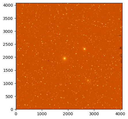
zero_pix = dm.data[dm.data <= 0]
print(len(zero_pix))
10938
Next, let’s create our catalog. Let’s choose a brightness of 2 x 10⁻⁸ maggies (~19.25 AB magnitudes) for our source. Note that if you are injecting galaxies, then you will also need to supply the other parameters Roman I-Sim needs for galaxy sources (e.g., Sérsic index and half-light radius).
In the next cell, we make a function for creating and saving our injection catalog:
# Define a function to create the catalog for sources
# that we want to inject into our L2 image.

def make_cat(ra, dec, fluxes, filename='injection_cat.ecsv'):

    filtlist = 'F062 F087 F106 F129 F146 F158 F184 F213'.split()
    tab = Table([ra, dec], names=('ra', 'dec'))
    src_types = np.array(['PSF' for i in ra])
    tab['type'] = src_types
    for k, v in fluxes.items():
        if k.upper() in filtlist:
            tab[k.upper()] = v
        else:
            raise ValueError(f'Incorrect filter name {k}!')

    tab.write(filename, overwrite=True)
And now run the function with our inputs:
# Get the RA and Dec from the WCS
ra, dec = dm.meta.wcs(1000, 1000)

# Make the injection catalog
make_cat([ra], [dec], {'F106': [2e-8]})
Let’s take a look at the catalog we just created and make sure it looks correct:
tab = Table.read('injection_cat.ecsv')
tab
| ra | dec | type | F106 |
|---|---|---|---|
| float64 | float64 | str3 | float64 |
| 270.69231500459955 | -0.14630904322742877 | PSF | 2e-08 |
Previously in this tutorial, we wrote a function to run Roman I-Sim. In that function, we overrode all of the default parameters and set them to None to force Roman I-Sim to use calibration reference files from CRDS rather than the Roman I-Sim default scalar values. These default scalar values are intended to allow Roman I-Sim to in an offline mode when you may not have access to a CRDS cache or the CRDS server. However, the current version of the inject_sources_into_l2() function does not use CRDS reference files and must use the Roman I-Sim defaults. Because the injection needs the default parameter values, we need to restore them here. We accomplish that using Python’s importlib.reload() function to reload the installed version of romanisim.parameters into memory:
importlib.reload(parameters)
<module 'romanisim.parameters' from '/home/runner/micromamba/envs/ci-env/lib/python3.13/site-packages/romanisim/parameters.py'>
Now we run the source injection function inject_sources_into_l2() with our image (datamodel), the injection catalog (the variable tab), and we set stpsf=True to use STPSF-generated point spread functions (PSFs) for the simulation. Notice that we make a copy of the image using the .copy() method so that we inject the source into a copy of the image rather than the original. This lets us compare the original and the updated version after we inject the source.
As a reminder, this will use the default Roman I-Sim parameter values for the injected source; however, perhaps the most critical parameter (the gain) can be modified in the function call. The gain is important in the simulation as the WFI zeropoints in the L2 metadata are intended to transform from DN/s to MJy/sr, and therefore contain a factor of the gain. If needed, the gain value used in the zeropoint can be found in the photom reference file. In the cell below, we will set the gain to the default value (2 e–/DN).
result = inject_sources_into_l2(dm.copy(), tab, psftype="stpsf", gain=2)
2026-06-01 20:03:45 INFO Creating PSF using stpsf
2026-06-01 20:03:45 INFO Using pupil mask 'F062' and detector 'WFI01'.
2026-06-01 20:03:45 INFO Using pupil mask 'F062' and detector 'WFI01'.
2026-06-01 20:03:45 INFO Using pupil mask 'F106' and detector 'WFI01'.
2026-06-01 20:03:45 INFO No source spectrum supplied, therefore defaulting to 5700 K blackbody
2026-06-01 20:03:45 INFO Computing wavelength weights using synthetic photometry for F106...
2026-06-01 20:03:45 INFO Using pupil mask 'F106' and detector 'WFI01'.
2026-06-01 20:03:45 INFO PSF calc using fov_arcsec = 5.000000, oversample = 4, number of wavelengths = 10
2026-06-01 20:03:45 INFO Creating optical system model:
2026-06-01 20:03:45 INFO Initialized OpticalSystem: Roman+WFI
2026-06-01 20:03:45 INFO Roman Entrance Pupil: Loaded amplitude transmission from /home/runner/refdata/stpsf-data/WFI/pupils/RST_WIM_Filter_F106_WFI01.fits.gz
2026-06-01 20:03:45 INFO Roman Entrance Pupil: Loaded OPD from /home/runner/refdata/stpsf-data/upscaled_HST_OPD.fits
2026-06-01 20:03:45 INFO Added pupil plane: Roman Entrance Pupil
2026-06-01 20:03:45 INFO Added coordinate inversion plane: OTE exit pupil
2026-06-01 20:03:45 INFO Added pupil plane: Field Dependent Aberration (WFI01)
2026-06-01 20:03:45 INFO Added detector with pixelscale=0.1078577405 and oversampling=4: WFI detector
2026-06-01 20:03:45 INFO Calculating PSF with 10 wavelengths
2026-06-01 20:03:45 INFO Propagating wavelength = 9.4555e-07 m
2026-06-01 20:03:46 INFO Propagating wavelength = 9.7265e-07 m
2026-06-01 20:03:46 INFO Propagating wavelength = 9.9975e-07 m
2026-06-01 20:03:46 INFO Propagating wavelength = 1.02685e-06 m
2026-06-01 20:03:47 INFO Propagating wavelength = 1.05395e-06 m
2026-06-01 20:03:47 INFO Propagating wavelength = 1.08105e-06 m
2026-06-01 20:03:47 INFO Propagating wavelength = 1.10815e-06 m
2026-06-01 20:03:48 INFO Propagating wavelength = 1.13525e-06 m
2026-06-01 20:03:48 INFO Propagating wavelength = 1.16235e-06 m
2026-06-01 20:03:48 INFO Propagating wavelength = 1.18945e-06 m
2026-06-01 20:03:49 INFO Calculation completed in 3.212 s
2026-06-01 20:03:49 INFO PSF Calculation completed.
2026-06-01 20:03:49 INFO Calculating jitter using gaussian
2026-06-01 20:03:49 INFO Jitter: Convolving with Gaussian with sigma=0.012 arcsec
2026-06-01 20:03:49 INFO resulting image peak drops to 0.946 of its previous value
2026-06-01 20:03:49 INFO Detector charge diffusion not applied because charge_diffusion_sigma option is 0
2026-06-01 20:03:49 INFO Adding extension with image downsampled to detector pixel scale.
2026-06-01 20:03:49 INFO Downsampling to detector pixel scale, by 4
2026-06-01 20:03:49 INFO Downsampling to detector pixel scale, by 4
2026-06-01 20:03:49 INFO Adding 1 sources to image...
2026-06-01 20:03:49 WARNING You requested fastpointsources, but the PSF and/or chromaticity are incompatible with this setting. Disabling fastpointsources.
2026-06-01 20:03:49 INFO Rendered 0 point sources in 0.00794 seconds
2026-06-01 20:03:49 INFO Rendered 1 total sources in 0.0318 seconds
2026-06-01 20:03:49 INFO Fitting ramps.
Finally, let’s re-plot the same region as before to show the injected source:
fig, axs = plt.subplots(nrows=1, ncols=2)

axs[0].imshow(dm.data[900:1100, 900:1100], norm=norm,
              cmap='afmhot', origin='lower',
              extent=[900, 1100, 900, 1100])

axs[0].set_title('Original')

axs[1].imshow(result.data[900:1100, 900:1100], norm=norm,
              cmap='afmhot', origin='lower',
              extent=[900, 1100, 900, 1100])

axs[1].set_title('Injected')

plt.tight_layout()
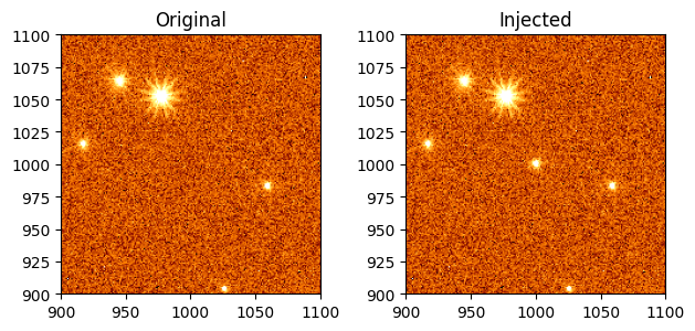
Additional Resources#
What is next#
Explore the Roman WFI data products with the Working with ASDF notebook.
Process Roman WFI raw (L1) data into exposure-level (L2) products using RomanCal with the Exposure Pipeline notebook.
Visualize Roman WFI exposure-level products using the Data Visualization notebook.
Combine multiple exposure-level (L2) products into mosaic-level (L3) images using the Mosaic Pipeline
About this Notebook#
Author: Sanjib Sharma, Tyler Desjardins, Rosa Diaz
Updated On: 2026-04-28
| Top of page |
|
|