
MIRI Coronagraphy Pipeline Notebook#
Authors: B. Nickson; MIRI branch, A. L. Carter; NIRISS branch
Last Updated: April 17, 2026
Pipeline Version: 2.0.0 (Build 12.3)
Purpose:
This notebook provides a framework for processing generic Mid-Infrared Instrument (MIRI) Coronagraphic data through all three James Webb Space Telescope (JWST) pipeline stages. Data is assumed to be located in separate observation folders according to the paths set up below. Editing cells other than those in the Configuration should not be necessary unless the standard pipeline processing options are modified.
Data:
This example is set up to use F1550C coronagraphic observations of the super-Jupiter exoplanet HIP 65426 b, obtained by Program ID 1386 (PI: S. Hinkley). It incorporates observations of the exoplanet host star HIP 65426 at two separate roll angles (1 exposure each); a PSF reference observation of the nearby star HIP 65219, taken with a 9-pt small grid dither pattern (9 exposures total); a background observation associated with the target star, taken with a 2-pt dither (two exposures); and a background observation associated with the PSF reference target, taken with a 2-pt dither (two exposures).
The relevant observation numbers are:
Science observations: 8, 9
Science backgrounds: 30
Reference observations: 7
Reference backgrounds: 31
Example input data to use will be downloaded automatically unless disabled (i.e., to use local files instead).
JWST pipeline version and CRDS context:
This notebook was written for the above-specified pipeline version and associated build context for this version of the JWST Calibration Pipeline. Information about this and other contexts can be found in the JWST Calibration Reference Data System (CRDS server). If you use different pipeline versions, please refer to the table here to determine what context to use. To learn more about the differences for the pipeline, read the relevant documentation.
Please note that pipeline software development is a continuous process, so results in some cases may be slightly different if a subsequent version is used. For optimal results, users are strongly encouraged to reprocess their data using the most recent pipeline version and associated CRDS context, taking advantage of bug fixes and algorithm improvements. Any known issues for this build are noted in the notebook.
Updates:
This notebook is regularly updated as improvements are made to the pipeline. Find the most up to date version of this notebook at:
spacetelescope/jwst-pipeline-notebooks
Recent Changes:
Jan 28, 2025: Migrate from the Coronagraphy_ExampleNB notebook, update to Build 11.2 (jwst 1.17.1).
May 5, 2025: Updated to jwst 1.18.0 (no significant changes)
July 16, 2025: Updated to jwst 1.19.1 (no significant changes)
November 10, 2025: Updated to jwst 1.20.2 (no significant changes)
March 27, 2026: Updated to demonstrate PSF library subtraction
April 17, 2026: Updated to jwst 2.0.0 (no significant changes)
Table of Contents#
1.-Configuration#
Set basic parameters to use with this notebook. These will affect what data is used, where data is located (if already in disk), and pipeline modules run on this data. The list of parameters are as follows:
demo_mode
directories with data
mask
filter
pipeline modules
# Basic import necessary for configuration
import os
demo_mode must be set appropriately below.
Set demo_mode = True to run in demonstration mode. In this mode, this
notebook will download example data from the
Barbara A. Mikulski Archive for Space Telescopes (MAST) and process it through the pipeline.
This will all happen in a local directory unless modified
in Section 3 below.
Set demo_mode = False if you want to process your own data that has already
been downloaded and provide the location of the data.
# Set parameters for demo_mode, mask, filter, data mode directories, and
# processing steps.

# -------------------------------Demo Mode---------------------------------
demo_mode = True

if demo_mode:
    print('Running in demonstration mode using online example data!')

# -------------------------Data Mode Directories---------------------------
# If demo_mode = False, look for user data in these paths
if not demo_mode:
    # Set directory paths for processing specific data; these will need
    # to be changed to your local directory setup (below are given as
    # examples)
    basedir = os.path.join(os.path.expanduser('~'), 'FlightData1386/')

    # Point to where science observation data are
    # Assumes uncalibrated data in sci_r1_dir/uncal/ and sci_r2_dir/uncal/,
    # and results in stage1, stage2, stage3 directories
    sci_r1_dir = os.path.join(basedir, 'sci_r1/')
    sci_r2_dir = os.path.join(basedir, 'sci_r2/')

    # Point to where reference target observation data are
    # Assumes uncalibrated data in ref_dir/uncal/ and results in stage1,
    # stage2, stage3 directories
    ref_targ_dir = os.path.join(basedir, 'ref_targ/')

    # Point to where background observation data are
    # Assumes uncalibrated data in sci_bg_dir/uncal/ and ref_targ_bg_dir/uncal/,
    # and results in stage1, stage2 directories
    bg_sci_dir = os.path.join(basedir, 'bg_sci/')
    bg_ref_targ_dir = os.path.join(basedir, 'bg_ref_targ/')

# --------------------------Set Processing Steps--------------------------
# Whether or not to process only data from a given coronagraphic mask/
# filter (useful if overriding reference files)
# Note that BOTH parameters must be set in order to work
use_mask = '4QPM_1550'  # '4QPM_1065', '4QPM_1140', '4QPM_1550', or 'LYOT_2300'
use_filter = 'F1550C'  # 'F1065C', 'F1140C', 'F1550C', or 'F2300C'

# Individual pipeline stages can be turned on/off here. Note that a later
# stage won't be able to run unless data products have already been
# produced from the prior stage.

# Science processing
dodet1 = True  # calwebb_detector1
doimage2 = True  # calwebb_image2
docoron3 = True  # calwebb_coron3
docoron3_psflib = True #calwebb_coron3 with larger PSF library

# Background processing
dodet1bg = True  # calwebb_detector1
doimage2bg = True  # calwebb_image2
Running in demonstration mode using online example data!
Set CRDS context and server#
Before importing CRDS and JWST modules, we need to configure our environment. This includes defining a CRDS cache directory in which to keep the reference files that will be used by the calibration pipeline.
If the root directory for the local CRDS cache directory has not been set already, it will be set to create one in the home directory.
# ------------------------Set CRDS context and paths----------------------
# Each version of the calibration pipeline is associated with a specific CRDS
# context file. The pipeline will select the appropriate context file behind
# the scenes while running. However, if you wish to override the default context
# file and run the pipeline with a different context, you can set that using
# the CRDS_CONTEXT environment variable. Here we show how this is done,
# although we leave the line commented out in order to use the default context.
# If you wish to specify a different context, uncomment the line below.
#%env CRDS_CONTEXT jwst_1322.pmap

# Check whether the local CRDS cache directory has been set.
# If not, set it to the user home directory
if (os.getenv('CRDS_PATH') is None):
    os.environ['CRDS_PATH'] = os.path.join(os.path.expanduser('~'), 'crds')

# Check whether the CRDS server URL has been set.  If not, set it.
if (os.getenv('CRDS_SERVER_URL') is None):
    os.environ['CRDS_SERVER_URL'] = 'https://jwst-crds.stsci.edu'

# Echo CRDS path in use
print('CRDS local filepath:', os.environ['CRDS_PATH'])
print('CRDS file server:', os.environ['CRDS_SERVER_URL'])
CRDS local filepath: /home/runner/crds
CRDS file server: https://jwst-crds.stsci.edu
2.-Package Imports#
# Use the entire available screen width for this notebook
from IPython.display import display, HTML
display(HTML("<style>.container { width:95% !important; }</style>"))
# Basic system utilities for interacting with files
# ----------------------General Imports------------------------------------
import glob, importlib
#import copy
import time
from pathlib import Path
from collections import defaultdict
import re

# Numpy for doing calculations
import numpy as np

# -----------------------Astropy Imports-----------------------------------
# Astropy utilities for opening FITS and ASCII files, and downloading demo files
from astropy.io import fits
from astropy.wcs import WCS
from astropy.coordinates import SkyCoord

#from astropy import time
from astroquery.mast import Observations

# -----------------------Plotting Imports----------------------------------
# Matplotlib for making plots
import matplotlib.pyplot as plt
# --------------JWST Calibration Pipeline Imports---------------------------
# Import the base JWST and calibration reference files packages
import jwst
import crds

# JWST pipelines (each encompassing many steps)
from jwst.pipeline import Detector1Pipeline
from jwst.pipeline import Image2Pipeline
from jwst.pipeline import Coron3Pipeline

# JWST pipeline utilities
from jwst import datamodels  # JWST datamodels
from jwst.associations import asn_from_list as afl  # Tools for creating association files
from jwst.associations.lib.rules_level2_base import DMSLevel2bBase  # Definition of a Lvl2 association file
from jwst.associations.lib.rules_level3_base import DMS_Level3_Base  # Definition of a Lvl3 association file

from jwst.stpipe import Step  # Import the wrapper class for pipeline steps

# Echo pipeline version and CRDS context in use
print("JWST Calibration Pipeline Version = {}".format(jwst.__version__))
print("Using CRDS Context = {}".format(crds.get_context_name('jwst')))
JWST Calibration Pipeline Version = 2.0.0
CRDS - INFO - Calibration SW Found: jwst 2.0.0 (/home/runner/micromamba/envs/ci-env/lib/python3.13/site-packages/jwst-2.0.0.dist-info)
Using CRDS Context = jwst_1535.pmap
Define convenience functions#
Define a convenience function to select only files of a given coronagraph mask/filter from an input set
# Define a convenience function to select only files of a given coronagraph mask/filter from an input set
def select_mask_filter_files(files, use_mask, use_filter):
    """
    Filter FITS files based on mask and filter criteria from their headers.

    Parameters:
    -----------
    files : array-like
        List of FITS file paths to process
    use_mask : str
        Mask value to match in FITS header 'CORONMSK' key
    use_filter : str
        Filter value to match in FITS header 'FILTER' key

    Returns:
    --------
    numpy.ndarray
        Filtered array of file paths matching the criteria
    """

    # Make paths absolute paths
    for i in range(len(files)):
        files[i] = os.path.abspath(files[i])

    # Convert files to numpy array if it isn't already
    files = np.asarray(files)

    # If either mask or filter is empty, return all files
    if not use_mask or not use_filter:
        return files

    try:
        # Initialize boolean array for keeping track of matches
        keep = np.zeros(len(files), dtype=bool)

        # Process each file
        for i in range(len(files)):
            try:
                with fits.open(files[i]) as hdu:
                    hdu.verify()
                    hdr = hdu[0].header

                    # Check if requred header keywords exist
                    if ('CORONMSK' in hdr and 'FILTER' in hdr):
                        if hdr['CORONMSK'] == use_mask and hdr['FILTER'] == use_filter:
                            keep[i] = True
                            files[i] = os.path.abspath(files[i])
            except (OSError, ValueError) as e:
                print(f" Warning: could not process file {files[i]}: {str(e)}")

        # Return filtered files
        indx = np.where(keep)
        return files[indx]

    except Exception as e:
        print(f"Error processing files: {str(e)}")
        return files  # Return original array in case of failure
# Start a timer to keep track of runtime
time0 = time.perf_counter()
3.-Demo Mode Setup (ignore if not using demo data)#
If running in demonstration mode, set up the program information to
retrieve the uncalibrated data automatically from MAST using
astroquery.
MAST allows for flexibility of searching by the proposal ID and the
observation ID instead of just filenames.
For illustrative purposes, we focus on data taken through the MIRI
F1550C filter
and start with uncalibrated raw data products (uncal.fits). The files use the following naming schema:
jw01386<obs>001_04101_0000<dith>_mirimage_uncal.fits, where obs refers to the observation number and dith refers to the
dither step number.
More information about the JWST file naming conventions can be found at: https://jwst-pipeline.readthedocs.io/en/latest/jwst/data_products/file_naming.html
# Set up the program information and paths for demo program
if demo_mode:
    print('Running in demonstration mode and will download example data from MAST!')
    program = "01386"
    sci_r1_observtn = "008"
    sci_r2_observtn = "009"
    ref_targ_observtn = "007"
    bg_sci_observtn = "030"
    bg_ref_targ_observtn = "031"

    # ----------Define the base and observation directories----------
    basedir = os.path.join('.', 'miri_coro_demo_data')
    download_dir = basedir
    sci_r1_dir = os.path.join(basedir, 'Obs' + sci_r1_observtn)
    sci_r2_dir = os.path.join(basedir, 'Obs' + sci_r2_observtn)
    ref_targ_dir = os.path.join(basedir, 'Obs' + ref_targ_observtn)
    bg_sci_dir = os.path.join(basedir, 'Obs' + bg_sci_observtn)
    bg_ref_targ_dir = os.path.join(basedir, 'Obs' + bg_ref_targ_observtn)

    uncal_sci_r1_dir = os.path.join(sci_r1_dir, 'uncal')
    uncal_sci_r2_dir = os.path.join(sci_r2_dir, 'uncal')
    uncal_ref_targ_dir = os.path.join(ref_targ_dir, 'uncal')
    uncal_bg_sci_dir = os.path.join(bg_sci_dir, 'uncal')
    uncal_bg_ref_targ_dir = os.path.join(bg_ref_targ_dir, 'uncal')

    # Ensure filepaths for input data exist
    input_dirs = [uncal_sci_r1_dir, uncal_sci_r2_dir, uncal_ref_targ_dir, uncal_bg_sci_dir, uncal_bg_ref_targ_dir]

    for dir in input_dirs:
        if not os.path.exists(dir):
            os.makedirs(dir)
Running in demonstration mode and will download example data from MAST!
Identify list of uncalibrated files associated with visits.
# Obtain a list of observation IDs for the specified demo program
if demo_mode:
    obs_id_table = Observations.query_criteria(instrument_name=["MIRI/CORON"],
                                               provenance_name=["CALJWST"],
                                               proposal_id=[program])
# Turn the list of visits into a list of uncalibrated data files
if demo_mode:
    # Define types of files to select
    file_dict = {'uncal': {'product_type': 'SCIENCE', 'productSubGroupDescription': 'UNCAL', 'calib_level': [1]}}

    # Loop over visits identifying uncalibrated files that are associated with them
    files_to_download = []
    for exposure in (obs_id_table):
        products = Observations.get_product_list(exposure)
        for filetype, query_dict in file_dict.items():
            filtered_products = Observations.filter_products(products, productType=query_dict['product_type'],
                                                             productSubGroupDescription=query_dict['productSubGroupDescription'],
                                                             calib_level=query_dict['calib_level'])
            files_to_download.extend(filtered_products['dataURI'])

    # Cull to a unique list of files for each observation type
    # Science roll 1
    sci_r1_files_to_download = []
    sci_r1_files_to_download = np.unique([i for i in files_to_download if str(program + sci_r1_observtn) in i])

    # Science roll 2
    sci_r2_files_to_download = []
    sci_r2_files_to_download = np.unique([i for i in files_to_download if str(program + sci_r2_observtn) in i])

    # PSF Reference taraget data
    ref_targ_files_to_download = []
    ref_targ_files_to_download = np.unique([i for i in files_to_download if str(program + ref_targ_observtn) in i])

    # Background files (science assoc.)
    bg_sci_files_to_download = []
    bg_sci_files_to_download = np.unique([i for i in files_to_download if str(program + bg_sci_observtn) in i])

    # Background files (reference target assoc.)
    bg_ref_targ_files_to_download = []
    bg_ref_targ_files_to_download = np.unique([i for i in files_to_download if str(program + bg_ref_targ_observtn) in i])

    print("Science files selected for downloading: ", len(sci_r1_files_to_download) + len(sci_r1_files_to_download))
    print("PSF Reference target files selected for downloading: ", len(ref_targ_files_to_download))
    print("Background selected for downloading: ", len(bg_sci_files_to_download) + len(bg_ref_targ_files_to_download))
Science files selected for downloading:  6
PSF Reference target files selected for downloading:  11
Background selected for downloading:  4
For the demo example, there should be 6 Science files, 11 PSF Reference files and 4 Background files selected for downloading.
Download all the uncal files and place them into the appropriate directories.
if demo_mode:
    for filename in sci_r1_files_to_download:
        sci_r1_manifest = Observations.download_file(filename, local_path=os.path.join(uncal_sci_r1_dir, Path(filename).name))
    for filename in sci_r2_files_to_download:
        sci_r2_manifest = Observations.download_file(filename, local_path=os.path.join(uncal_sci_r2_dir, Path(filename).name))
    for filename in ref_targ_files_to_download:
        ref_targ_manifest = Observations.download_file(filename, local_path=os.path.join(uncal_ref_targ_dir, Path(filename).name))
    for filename in bg_sci_files_to_download:
        bg_manifest = Observations.download_file(filename, local_path=os.path.join(uncal_bg_sci_dir, Path(filename).name))
    for filename in bg_ref_targ_files_to_download:
        bg_ref_targ_manifest = Observations.download_file(filename, local_path=os.path.join(uncal_bg_ref_targ_dir, Path(filename).name))
Downloading URL https://mast.stsci.edu/api/v0.1/Download/file?uri=mast:JWST/product/jw01386008001_02101_00001_mirimage_uncal.fits to ./miri_coro_demo_data/Obs008/uncal/jw01386008001_02101_00001_mirimage_uncal.fits ...
[Done]
Downloading URL https://mast.stsci.edu/api/v0.1/Download/file?uri=mast:JWST/product/jw01386008001_02101_00002_mirimage_uncal.fits to ./miri_coro_demo_data/Obs008/uncal/jw01386008001_02101_00002_mirimage_uncal.fits ...
[Done]
Downloading URL https://mast.stsci.edu/api/v0.1/Download/file?uri=mast:JWST/product/jw01386008001_04101_00001_mirimage_uncal.fits to ./miri_coro_demo_data/Obs008/uncal/jw01386008001_04101_00001_mirimage_uncal.fits ...
[Done]
Downloading URL https://mast.stsci.edu/api/v0.1/Download/file?uri=mast:JWST/product/jw01386009001_02101_00001_mirimage_uncal.fits to ./miri_coro_demo_data/Obs009/uncal/jw01386009001_02101_00001_mirimage_uncal.fits ...
[Done]
Downloading URL https://mast.stsci.edu/api/v0.1/Download/file?uri=mast:JWST/product/jw01386009001_02101_00002_mirimage_uncal.fits to ./miri_coro_demo_data/Obs009/uncal/jw01386009001_02101_00002_mirimage_uncal.fits ...
[Done]
Downloading URL https://mast.stsci.edu/api/v0.1/Download/file?uri=mast:JWST/product/jw01386009001_04101_00001_mirimage_uncal.fits to ./miri_coro_demo_data/Obs009/uncal/jw01386009001_04101_00001_mirimage_uncal.fits ...
[Done]
Downloading URL https://mast.stsci.edu/api/v0.1/Download/file?uri=mast:JWST/product/jw01386007001_02101_00001_mirimage_uncal.fits to ./miri_coro_demo_data/Obs007/uncal/jw01386007001_02101_00001_mirimage_uncal.fits ...
[Done]
Downloading URL https://mast.stsci.edu/api/v0.1/Download/file?uri=mast:JWST/product/jw01386007001_02101_00002_mirimage_uncal.fits to ./miri_coro_demo_data/Obs007/uncal/jw01386007001_02101_00002_mirimage_uncal.fits ...
[Done]
Downloading URL https://mast.stsci.edu/api/v0.1/Download/file?uri=mast:JWST/product/jw01386007001_04101_00001_mirimage_uncal.fits to ./miri_coro_demo_data/Obs007/uncal/jw01386007001_04101_00001_mirimage_uncal.fits ...
[Done]
Downloading URL https://mast.stsci.edu/api/v0.1/Download/file?uri=mast:JWST/product/jw01386007001_04101_00002_mirimage_uncal.fits to ./miri_coro_demo_data/Obs007/uncal/jw01386007001_04101_00002_mirimage_uncal.fits ...
[Done]
Downloading URL https://mast.stsci.edu/api/v0.1/Download/file?uri=mast:JWST/product/jw01386007001_04101_00003_mirimage_uncal.fits to ./miri_coro_demo_data/Obs007/uncal/jw01386007001_04101_00003_mirimage_uncal.fits ...
[Done]
Downloading URL https://mast.stsci.edu/api/v0.1/Download/file?uri=mast:JWST/product/jw01386007001_04101_00004_mirimage_uncal.fits to ./miri_coro_demo_data/Obs007/uncal/jw01386007001_04101_00004_mirimage_uncal.fits ...
[Done]
Downloading URL https://mast.stsci.edu/api/v0.1/Download/file?uri=mast:JWST/product/jw01386007001_04101_00005_mirimage_uncal.fits to ./miri_coro_demo_data/Obs007/uncal/jw01386007001_04101_00005_mirimage_uncal.fits ...
[Done]
Downloading URL https://mast.stsci.edu/api/v0.1/Download/file?uri=mast:JWST/product/jw01386007001_04101_00006_mirimage_uncal.fits to ./miri_coro_demo_data/Obs007/uncal/jw01386007001_04101_00006_mirimage_uncal.fits ...
[Done]
Downloading URL https://mast.stsci.edu/api/v0.1/Download/file?uri=mast:JWST/product/jw01386007001_04101_00007_mirimage_uncal.fits to ./miri_coro_demo_data/Obs007/uncal/jw01386007001_04101_00007_mirimage_uncal.fits ...
[Done]
Downloading URL https://mast.stsci.edu/api/v0.1/Download/file?uri=mast:JWST/product/jw01386007001_04101_00008_mirimage_uncal.fits to ./miri_coro_demo_data/Obs007/uncal/jw01386007001_04101_00008_mirimage_uncal.fits ...
[Done]
Downloading URL https://mast.stsci.edu/api/v0.1/Download/file?uri=mast:JWST/product/jw01386007001_04101_00009_mirimage_uncal.fits to ./miri_coro_demo_data/Obs007/uncal/jw01386007001_04101_00009_mirimage_uncal.fits ...
[Done]
Downloading URL https://mast.stsci.edu/api/v0.1/Download/file?uri=mast:JWST/product/jw01386030001_02101_00001_mirimage_uncal.fits to ./miri_coro_demo_data/Obs030/uncal/jw01386030001_02101_00001_mirimage_uncal.fits ...
[Done]
Downloading URL https://mast.stsci.edu/api/v0.1/Download/file?uri=mast:JWST/product/jw01386030001_03101_00001_mirimage_uncal.fits to ./miri_coro_demo_data/Obs030/uncal/jw01386030001_03101_00001_mirimage_uncal.fits ...
[Done]
Downloading URL https://mast.stsci.edu/api/v0.1/Download/file?uri=mast:JWST/product/jw01386031001_02101_00001_mirimage_uncal.fits to ./miri_coro_demo_data/Obs031/uncal/jw01386031001_02101_00001_mirimage_uncal.fits ...
[Done]
Downloading URL https://mast.stsci.edu/api/v0.1/Download/file?uri=mast:JWST/product/jw01386031001_03101_00001_mirimage_uncal.fits to ./miri_coro_demo_data/Obs031/uncal/jw01386031001_03101_00001_mirimage_uncal.fits ...
[Done]
4.-Directory Setup#
Set up detailed paths to input/output stages here. We will set up individual stage1/ and stage2/ sub directories for each observation, but a single stage3/ directory for the combined calwebb_coron3 output products.
# Define output subdirectories to keep science data products organized
# Sci Roll 1
uncal_sci_r1_dir = os.path.join(sci_r1_dir, 'uncal') # uncal inputs go here
det1_sci_r1_dir = os.path.join(sci_r1_dir, 'stage1')  # calwebb_detector1 pipeline outputs will go here
image2_sci_r1_dir = os.path.join(sci_r1_dir, 'stage2')  # calwebb_image2 pipeline outputs will go here

# Sci Roll 2
uncal_sci_r2_dir = os.path.join(sci_r2_dir, 'uncal') # uncal inputs go here
det1_sci_r2_dir = os.path.join(sci_r2_dir, 'stage1')  # calwebb_detector1 pipeline outputs will go here
image2_sci_r2_dir = os.path.join(sci_r2_dir, 'stage2')  # calwebb_image2 pipeline outputs will go here

# Define output subdirectories to keep PSF reference target data products organized
uncal_ref_targ_dir = os.path.join(ref_targ_dir, 'uncal') # uncal inputs go here
det1_ref_targ_dir = os.path.join(ref_targ_dir, 'stage1')  # calwebb_detector1 pipeline outputs will go here
image2_ref_targ_dir = os.path.join(ref_targ_dir, 'stage2')  # calwebb_image2 pipeline outputs will go here

# Define output subdirectories to keep background data products organized
# Sci Bkg
uncal_bg_sci_dir = os.path.join(bg_sci_dir, 'uncal') # uncal inputs go here
det1_bg_sci_dir = os.path.join(bg_sci_dir, 'stage1')  # calwebb_detector1 pipeline outputs will go here
image2_bg_sci_dir = os.path.join(bg_sci_dir, 'stage2')  # calwebb_image2 pipeline outputs will go here

# Ref target Bkg
uncal_bg_ref_targ_dir = os.path.join(bg_ref_targ_dir, 'uncal') # uncal inputs go here
det1_bg_ref_targ_dir = os.path.join(bg_ref_targ_dir, 'stage1')  # calwebb_detector1 pipeline outputs will go here
image2_bg_ref_targ_dir = os.path.join(bg_ref_targ_dir, 'stage2')  # calwebb_image2 pipeline outputs will go here

coron3_dir = os.path.join(basedir, 'stage3')
coron3_psflib_dir = os.path.join(basedir, 'stage3_psflib/') # calwebb_coron3 pipeline outputs using the PSF library will go here

# We need to check that the desired output directories exist, and if not create them
det1_dirs = [det1_sci_r1_dir, det1_sci_r2_dir, det1_ref_targ_dir, det1_bg_sci_dir, det1_bg_ref_targ_dir]
image2_dirs = [image2_sci_r1_dir, image2_sci_r2_dir, image2_ref_targ_dir, image2_bg_sci_dir, image2_bg_ref_targ_dir]

for dir in det1_dirs:
    if not os.path.exists(dir):
        os.makedirs(dir)
for dir in image2_dirs:
    if not os.path.exists(dir):
        os.makedirs(dir)
if not os.path.exists(coron3_dir):
    os.makedirs(coron3_dir)
if not os.path.exists(coron3_psflib_dir):
    os.makedirs(coron3_psflib_dir)
# Print out the time benchmark
time1 = time.perf_counter()
print(f"Runtime so far: {time1 - time0:0.4f} seconds")
Runtime so far: 298.9818 seconds
5.-Detector1 Pipeline#
In this section, we process our uncalibrated data through the calwebb_detector1 pipeline to create Stage 1 data products. For coronagraphic exposures, these data products include a *_rate.fits file (a 2D countrate product, based on averaging over all integrations in the exposure), but specifically also a *_rateints.fits file, a 3D countrate product, that contains the individual results of each integration, wherein 2D countrate images for each integration are stacked along the 3rd axis of the data cubes (ncols x nrows x nints). These data products have units of DN/s.
See https://jwst-docs.stsci.edu/jwst-science-calibration-pipeline/stages-of-jwst-data-processing/calwebb_detector1
By default, all steps in the calwebb_detector1 are run for MIRI except: the ipc and charge_migration steps. There are also several steps performed for MIRI data that are not performed for other instruments. These include: emicorr, firstframe, lastframe, reset and rscd.
E.g., turn on detection of cosmic ray showers.
# Set up a dictionary to define how the Detector1 pipeline should be configured

# Boilerplate dictionary setup
det1dict = defaultdict(dict)

# Overrides for whether or not certain steps should be skipped (example)
# skipping refpix step
#det1dict['refpix']['skip'] = True

# Overrides for various reference files
# Files should be in the base local directory or provide full path
#det1dict['dq_init']['override_mask'] = 'myfile.fits' # Bad pixel mask
#det1dict['saturation']['override_saturation'] = 'myfile.fits'  # Saturation
#det1dict['reset']['override_reset'] = 'myfile.fits'  # Reset
#det1dict['linearity']['override_linearity'] = 'myfile.fits'  # Linearity
#det1dict['rscd']['override_rscd'] = 'myfile.fits'  # RSCD
#det1dict['dark_current']['override_dark'] = 'myfile.fits'  # Dark current subtraction
#det1dict['jump']['override_gain'] = 'myfile.fits'  # Gain used by jump step
#det1dict['ramp_fit']['override_gain'] = 'myfile.fits'  # Gain used by ramp fitting step
#det1dict['jump']['override_readnoise'] = 'myfile.fits'  # Read noise used by jump step
#det1dict['ramp_fit']['override_readnoise'] = 'myfile.fits'  # Read noise used by ramp fitting step

# Turn on multi-core processing (off by default).  Choose what fraction of cores to use (quarter, half, or all)
det1dict['jump']['maximum_cores'] = 'half'

# Save the frame-averaged dark data created during the dark current subtraction step
#det1dict['dark_current']['dark_output'] = 'dark.fits'  # Frame-averaged dark

# Turn on detection of cosmic ray showers (off by default)
#det1dict['jump']['find_showers'] = True
For more information see Tips and Trick for working with the JWST Pipeline
# Define a new step called XplyStep that multiplies everything by 1.0
# I.e., it does nothing, but could be changed to do something more interesting.
class XplyStep(Step):
    spec = '''
    '''
    class_alias = 'xply'

    def process(self, input_data):
        with datamodels.open(input_data) as model:
            result = model.copy()
        sci = result.data
        sci = sci * 1.0
        result.data = sci
        self.log.info('Multiplied everything by one in custom step!')
        return result


# And here we'll insert it into our pipeline dictionary to be run at the end right after the gain_scale step
det1dict['gain_scale']['post_hooks'] = [XplyStep]
# Let's also define a pre-hook for the ramp_fit step that sets the left, right, bottom, and top edges to DO_NOT_USE.
class EdgeMaskStep(Step):
    spec = '''
    '''
    class_alias = 'edgemask'

    def process(self, input_data):
        with datamodels.open(input_data) as model:
            result = model.copy()

        # For ramp_fit we want to flag groups as unusable, so operate on the 3-D
        # GROUPDQ array: (nint, ngroup, ny, nx)
        gdq = result.groupdq

        do_not_use = 2**0  # DQ flag bit 0
        mod = 50
        # Set left and right edges to DO_NOT_USE (all ints, all groups)
        gdq[:, :, :, 0:13+mod] = gdq[:, :, :, 0:13+mod] | do_not_use  # Left edge
        gdq[:, :, :, -60-mod:] = gdq[:, :, :, -60-mod:] | do_not_use  # Right edge

        # Set bottom and top edges to DO_NOT_USE
        gdq[:, :, 0:7+mod, :] = gdq[:, :, 0:7+mod, :] | do_not_use  # Bottom edge
        gdq[:, :, -7-mod:, :] = gdq[:, :, -7-mod:, :] | do_not_use  # Top edge

        result.groupdq = gdq
        self.log.info('Set the edges to DO_NOT_USE in custom pre-hook (GROUPDQ)!')
        return result

# det1dict['ramp_fit']['pre_hooks'] = [EdgeMaskStep]
Calibrating Science Files#
Look for input science files and run calwebb_detector1 pipeline using the call method. For the demo example there should be 2 input science files, one for the observation at roll 1 (Obs 8) and one for the observation at roll 2 (Obs 9).
uncal_sci_r1_dir
'./miri_coro_demo_data/Obs008/uncal'
# Look for input files of the form *uncal.fits from the science observation
sstring1 = os.path.join(uncal_sci_r1_dir, 'jw*mirimage*uncal.fits')
sstring2 = os.path.join(uncal_sci_r2_dir, 'jw*mirimage*uncal.fits')

uncal_sci_r1_files = sorted(glob.glob(sstring1))
uncal_sci_r2_files = sorted(glob.glob(sstring2))

# Check that these are the correct mask/filter to use
uncal_sci_r1_files = select_mask_filter_files(uncal_sci_r1_files, use_mask, use_filter)
uncal_sci_r2_files = select_mask_filter_files(uncal_sci_r2_files, use_mask, use_filter)

print('Found ' + str((len(uncal_sci_r1_files) + len(uncal_sci_r2_files))) + ' science input files')
Found 2 science input files
# Run the pipeline on these input files by a simple loop over files using
# our custom parameter dictionary
if dodet1:
    for file in uncal_sci_r1_files:
        Detector1Pipeline.call(file, steps=det1dict, save_results=True, output_dir=det1_sci_r1_dir)

    for file in uncal_sci_r2_files:
        Detector1Pipeline.call(file, steps=det1dict, save_results=True, output_dir=det1_sci_r2_dir)
else:
    print('Skipping Detector1 processing for SCI data')
2026-04-15 20:19:59,054 - CRDS - INFO - Fetching /home/runner/crds/mappings/jwst/jwst_system_datalvl_0002.rmap 694 bytes (1 / 224 files) (0 / 796.2 K bytes)
2026-04-15 20:19:59,266 - CRDS - INFO - Fetching /home/runner/crds/mappings/jwst/jwst_system_calver_0069.rmap 5.8 K bytes (2 / 224 files) (694 / 796.2 K bytes)
2026-04-15 20:19:59,494 - CRDS - INFO - Fetching /home/runner/crds/mappings/jwst/jwst_system_0064.imap 385 bytes (3 / 224 files) (6.5 K / 796.2 K bytes)
2026-04-15 20:19:59,725 - CRDS - INFO - Fetching /home/runner/crds/mappings/jwst/jwst_nirspec_wavelengthrange_0024.rmap 1.4 K bytes (4 / 224 files) (6.9 K / 796.2 K bytes)
2026-04-15 20:19:59,945 - CRDS - INFO - Fetching /home/runner/crds/mappings/jwst/jwst_nirspec_wavecorr_0005.rmap 884 bytes (5 / 224 files) (8.3 K / 796.2 K bytes)
2026-04-15 20:20:00,194 - CRDS - INFO - Fetching /home/runner/crds/mappings/jwst/jwst_nirspec_superbias_0089.rmap 39.4 K bytes (6 / 224 files) (9.1 K / 796.2 K bytes)
2026-04-15 20:20:00,503 - CRDS - INFO - Fetching /home/runner/crds/mappings/jwst/jwst_nirspec_sirskernel_0002.rmap 704 bytes (7 / 224 files) (48.5 K / 796.2 K bytes)
2026-04-15 20:20:00,738 - CRDS - INFO - Fetching /home/runner/crds/mappings/jwst/jwst_nirspec_sflat_0027.rmap 20.6 K bytes (8 / 224 files) (49.2 K / 796.2 K bytes)
2026-04-15 20:20:01,032 - CRDS - INFO - Fetching /home/runner/crds/mappings/jwst/jwst_nirspec_saturation_0018.rmap 2.0 K bytes (9 / 224 files) (69.8 K / 796.2 K bytes)
2026-04-15 20:20:01,268 - CRDS - INFO - Fetching /home/runner/crds/mappings/jwst/jwst_nirspec_refpix_0015.rmap 1.6 K bytes (10 / 224 files) (71.9 K / 796.2 K bytes)
2026-04-15 20:20:01,479 - CRDS - INFO - Fetching /home/runner/crds/mappings/jwst/jwst_nirspec_readnoise_0025.rmap 2.6 K bytes (11 / 224 files) (73.4 K / 796.2 K bytes)
2026-04-15 20:20:01,722 - CRDS - INFO - Fetching /home/runner/crds/mappings/jwst/jwst_nirspec_psf_0002.rmap 687 bytes (12 / 224 files) (76.0 K / 796.2 K bytes)
2026-04-15 20:20:01,942 - CRDS - INFO - Fetching /home/runner/crds/mappings/jwst/jwst_nirspec_pictureframe_0002.rmap 886 bytes (13 / 224 files) (76.7 K / 796.2 K bytes)
2026-04-15 20:20:02,172 - CRDS - INFO - Fetching /home/runner/crds/mappings/jwst/jwst_nirspec_photom_0013.rmap 958 bytes (14 / 224 files) (77.6 K / 796.2 K bytes)
2026-04-15 20:20:02,399 - CRDS - INFO - Fetching /home/runner/crds/mappings/jwst/jwst_nirspec_pathloss_0011.rmap 1.2 K bytes (15 / 224 files) (78.5 K / 796.2 K bytes)
2026-04-15 20:20:02,622 - CRDS - INFO - Fetching /home/runner/crds/mappings/jwst/jwst_nirspec_pars-whitelightstep_0001.rmap 777 bytes (16 / 224 files) (79.7 K / 796.2 K bytes)
2026-04-15 20:20:02,866 - CRDS - INFO - Fetching /home/runner/crds/mappings/jwst/jwst_nirspec_pars-tso3pipeline_0001.rmap 786 bytes (17 / 224 files) (80.5 K / 796.2 K bytes)
2026-04-15 20:20:03,077 - CRDS - INFO - Fetching /home/runner/crds/mappings/jwst/jwst_nirspec_pars-spec2pipeline_0013.rmap 2.1 K bytes (18 / 224 files) (81.3 K / 796.2 K bytes)
2026-04-15 20:20:03,308 - CRDS - INFO - Fetching /home/runner/crds/mappings/jwst/jwst_nirspec_pars-resamplespecstep_0002.rmap 709 bytes (19 / 224 files) (83.4 K / 796.2 K bytes)
2026-04-15 20:20:03,516 - CRDS - INFO - Fetching /home/runner/crds/mappings/jwst/jwst_nirspec_pars-refpixstep_0003.rmap 910 bytes (20 / 224 files) (84.1 K / 796.2 K bytes)
2026-04-15 20:20:03,749 - CRDS - INFO - Fetching /home/runner/crds/mappings/jwst/jwst_nirspec_pars-pixelreplacestep_0001.rmap 818 bytes (21 / 224 files) (85.0 K / 796.2 K bytes)
2026-04-15 20:20:03,974 - CRDS - INFO - Fetching /home/runner/crds/mappings/jwst/jwst_nirspec_pars-pictureframestep_0001.rmap 818 bytes (22 / 224 files) (85.8 K / 796.2 K bytes)
2026-04-15 20:20:04,183 - CRDS - INFO - Fetching /home/runner/crds/mappings/jwst/jwst_nirspec_pars-outlierdetectionstep_0005.rmap 1.1 K bytes (23 / 224 files) (86.7 K / 796.2 K bytes)
2026-04-15 20:20:04,396 - CRDS - INFO - Fetching /home/runner/crds/mappings/jwst/jwst_nirspec_pars-jumpstep_0006.rmap 810 bytes (24 / 224 files) (87.8 K / 796.2 K bytes)
2026-04-15 20:20:04,629 - CRDS - INFO - Fetching /home/runner/crds/mappings/jwst/jwst_nirspec_pars-image2pipeline_0008.rmap 1.0 K bytes (25 / 224 files) (88.6 K / 796.2 K bytes)
2026-04-15 20:20:04,873 - CRDS - INFO - Fetching /home/runner/crds/mappings/jwst/jwst_nirspec_pars-extract1dstep_0001.rmap 794 bytes (26 / 224 files) (89.6 K / 796.2 K bytes)
2026-04-15 20:20:05,105 - CRDS - INFO - Fetching /home/runner/crds/mappings/jwst/jwst_nirspec_pars-detector1pipeline_0004.rmap 1.1 K bytes (27 / 224 files) (90.4 K / 796.2 K bytes)
2026-04-15 20:20:05,324 - CRDS - INFO - Fetching /home/runner/crds/mappings/jwst/jwst_nirspec_pars-darkpipeline_0003.rmap 872 bytes (28 / 224 files) (91.5 K / 796.2 K bytes)
2026-04-15 20:20:05,534 - CRDS - INFO - Fetching /home/runner/crds/mappings/jwst/jwst_nirspec_pars-darkcurrentstep_0003.rmap 1.8 K bytes (29 / 224 files) (92.4 K / 796.2 K bytes)
2026-04-15 20:20:05,761 - CRDS - INFO - Fetching /home/runner/crds/mappings/jwst/jwst_nirspec_pars-cubebuildstep_0001.rmap 862 bytes (30 / 224 files) (94.2 K / 796.2 K bytes)
2026-04-15 20:20:05,982 - CRDS - INFO - Fetching /home/runner/crds/mappings/jwst/jwst_nirspec_pars-cleanflickernoisestep_0002.rmap 983 bytes (31 / 224 files) (95.1 K / 796.2 K bytes)
2026-04-15 20:20:06,211 - CRDS - INFO - Fetching /home/runner/crds/mappings/jwst/jwst_nirspec_pars-adaptivetracemodelstep_0002.rmap 997 bytes (32 / 224 files) (96.1 K / 796.2 K bytes)
2026-04-15 20:20:06,425 - CRDS - INFO - Fetching /home/runner/crds/mappings/jwst/jwst_nirspec_ote_0030.rmap 1.3 K bytes (33 / 224 files) (97.1 K / 796.2 K bytes)
2026-04-15 20:20:06,663 - CRDS - INFO - Fetching /home/runner/crds/mappings/jwst/jwst_nirspec_msaoper_0018.rmap 1.6 K bytes (34 / 224 files) (98.3 K / 796.2 K bytes)
2026-04-15 20:20:06,881 - CRDS - INFO - Fetching /home/runner/crds/mappings/jwst/jwst_nirspec_msa_0027.rmap 1.3 K bytes (35 / 224 files) (100.0 K / 796.2 K bytes)
2026-04-15 20:20:07,090 - CRDS - INFO - Fetching /home/runner/crds/mappings/jwst/jwst_nirspec_mask_0045.rmap 4.9 K bytes (36 / 224 files) (101.2 K / 796.2 K bytes)
2026-04-15 20:20:07,305 - CRDS - INFO - Fetching /home/runner/crds/mappings/jwst/jwst_nirspec_linearity_0017.rmap 1.6 K bytes (37 / 224 files) (106.2 K / 796.2 K bytes)
2026-04-15 20:20:07,516 - CRDS - INFO - Fetching /home/runner/crds/mappings/jwst/jwst_nirspec_ipc_0006.rmap 876 bytes (38 / 224 files) (107.7 K / 796.2 K bytes)
2026-04-15 20:20:07,726 - CRDS - INFO - Fetching /home/runner/crds/mappings/jwst/jwst_nirspec_ifuslicer_0018.rmap 1.5 K bytes (39 / 224 files) (108.6 K / 796.2 K bytes)
2026-04-15 20:20:07,960 - CRDS - INFO - Fetching /home/runner/crds/mappings/jwst/jwst_nirspec_ifupost_0020.rmap 1.5 K bytes (40 / 224 files) (110.1 K / 796.2 K bytes)
2026-04-15 20:20:08,169 - CRDS - INFO - Fetching /home/runner/crds/mappings/jwst/jwst_nirspec_ifufore_0017.rmap 1.5 K bytes (41 / 224 files) (111.6 K / 796.2 K bytes)
2026-04-15 20:20:08,386 - CRDS - INFO - Fetching /home/runner/crds/mappings/jwst/jwst_nirspec_gain_0023.rmap 1.8 K bytes (42 / 224 files) (113.1 K / 796.2 K bytes)
2026-04-15 20:20:08,602 - CRDS - INFO - Fetching /home/runner/crds/mappings/jwst/jwst_nirspec_fpa_0028.rmap 1.3 K bytes (43 / 224 files) (114.9 K / 796.2 K bytes)
2026-04-15 20:20:08,833 - CRDS - INFO - Fetching /home/runner/crds/mappings/jwst/jwst_nirspec_fore_0026.rmap 5.0 K bytes (44 / 224 files) (116.2 K / 796.2 K bytes)
2026-04-15 20:20:09,050 - CRDS - INFO - Fetching /home/runner/crds/mappings/jwst/jwst_nirspec_flat_0015.rmap 3.8 K bytes (45 / 224 files) (121.1 K / 796.2 K bytes)
2026-04-15 20:20:09,277 - CRDS - INFO - Fetching /home/runner/crds/mappings/jwst/jwst_nirspec_fflat_0030.rmap 7.2 K bytes (46 / 224 files) (124.9 K / 796.2 K bytes)
2026-04-15 20:20:09,487 - CRDS - INFO - Fetching /home/runner/crds/mappings/jwst/jwst_nirspec_extract1d_0018.rmap 2.3 K bytes (47 / 224 files) (132.1 K / 796.2 K bytes)
2026-04-15 20:20:09,716 - CRDS - INFO - Fetching /home/runner/crds/mappings/jwst/jwst_nirspec_disperser_0028.rmap 5.7 K bytes (48 / 224 files) (134.4 K / 796.2 K bytes)
2026-04-15 20:20:09,936 - CRDS - INFO - Fetching /home/runner/crds/mappings/jwst/jwst_nirspec_dflat_0007.rmap 1.1 K bytes (49 / 224 files) (140.1 K / 796.2 K bytes)
2026-04-15 20:20:10,144 - CRDS - INFO - Fetching /home/runner/crds/mappings/jwst/jwst_nirspec_dark_0085.rmap 37.4 K bytes (50 / 224 files) (141.3 K / 796.2 K bytes)
2026-04-15 20:20:10,433 - CRDS - INFO - Fetching /home/runner/crds/mappings/jwst/jwst_nirspec_cubepar_0015.rmap 966 bytes (51 / 224 files) (178.7 K / 796.2 K bytes)
2026-04-15 20:20:10,642 - CRDS - INFO - Fetching /home/runner/crds/mappings/jwst/jwst_nirspec_collimator_0026.rmap 1.3 K bytes (52 / 224 files) (179.6 K / 796.2 K bytes)
2026-04-15 20:20:10,879 - CRDS - INFO - Fetching /home/runner/crds/mappings/jwst/jwst_nirspec_camera_0026.rmap 1.3 K bytes (53 / 224 files) (181.0 K / 796.2 K bytes)
2026-04-15 20:20:11,110 - CRDS - INFO - Fetching /home/runner/crds/mappings/jwst/jwst_nirspec_barshadow_0007.rmap 1.8 K bytes (54 / 224 files) (182.3 K / 796.2 K bytes)
2026-04-15 20:20:11,318 - CRDS - INFO - Fetching /home/runner/crds/mappings/jwst/jwst_nirspec_area_0019.rmap 6.8 K bytes (55 / 224 files) (184.1 K / 796.2 K bytes)
2026-04-15 20:20:11,537 - CRDS - INFO - Fetching /home/runner/crds/mappings/jwst/jwst_nirspec_apcorr_0009.rmap 5.6 K bytes (56 / 224 files) (190.9 K / 796.2 K bytes)
2026-04-15 20:20:11,765 - CRDS - INFO - Fetching /home/runner/crds/mappings/jwst/jwst_nirspec_0432.imap 6.2 K bytes (57 / 224 files) (196.5 K / 796.2 K bytes)
2026-04-15 20:20:11,989 - CRDS - INFO - Fetching /home/runner/crds/mappings/jwst/jwst_niriss_wavelengthrange_0008.rmap 897 bytes (58 / 224 files) (202.6 K / 796.2 K bytes)
2026-04-15 20:20:12,204 - CRDS - INFO - Fetching /home/runner/crds/mappings/jwst/jwst_niriss_trappars_0004.rmap 753 bytes (59 / 224 files) (203.5 K / 796.2 K bytes)
2026-04-15 20:20:12,414 - CRDS - INFO - Fetching /home/runner/crds/mappings/jwst/jwst_niriss_trapdensity_0005.rmap 705 bytes (60 / 224 files) (204.3 K / 796.2 K bytes)
2026-04-15 20:20:12,645 - CRDS - INFO - Fetching /home/runner/crds/mappings/jwst/jwst_niriss_throughput_0005.rmap 1.3 K bytes (61 / 224 files) (205.0 K / 796.2 K bytes)
2026-04-15 20:20:12,884 - CRDS - INFO - Fetching /home/runner/crds/mappings/jwst/jwst_niriss_superbias_0035.rmap 8.3 K bytes (62 / 224 files) (206.2 K / 796.2 K bytes)
2026-04-15 20:20:13,094 - CRDS - INFO - Fetching /home/runner/crds/mappings/jwst/jwst_niriss_specwcs_0017.rmap 3.1 K bytes (63 / 224 files) (214.5 K / 796.2 K bytes)
2026-04-15 20:20:13,303 - CRDS - INFO - Fetching /home/runner/crds/mappings/jwst/jwst_niriss_specprofile_0010.rmap 2.5 K bytes (64 / 224 files) (217.7 K / 796.2 K bytes)
2026-04-15 20:20:13,513 - CRDS - INFO - Fetching /home/runner/crds/mappings/jwst/jwst_niriss_speckernel_0006.rmap 1.0 K bytes (65 / 224 files) (220.2 K / 796.2 K bytes)
2026-04-15 20:20:13,755 - CRDS - INFO - Fetching /home/runner/crds/mappings/jwst/jwst_niriss_sirskernel_0002.rmap 700 bytes (66 / 224 files) (221.2 K / 796.2 K bytes)
2026-04-15 20:20:13,965 - CRDS - INFO - Fetching /home/runner/crds/mappings/jwst/jwst_niriss_saturation_0015.rmap 829 bytes (67 / 224 files) (221.9 K / 796.2 K bytes)
2026-04-15 20:20:14,193 - CRDS - INFO - Fetching /home/runner/crds/mappings/jwst/jwst_niriss_readnoise_0011.rmap 987 bytes (68 / 224 files) (222.7 K / 796.2 K bytes)
2026-04-15 20:20:14,429 - CRDS - INFO - Fetching /home/runner/crds/mappings/jwst/jwst_niriss_photom_0041.rmap 1.3 K bytes (69 / 224 files) (223.7 K / 796.2 K bytes)
2026-04-15 20:20:14,640 - CRDS - INFO - Fetching /home/runner/crds/mappings/jwst/jwst_niriss_persat_0007.rmap 674 bytes (70 / 224 files) (225.0 K / 796.2 K bytes)
2026-04-15 20:20:14,860 - CRDS - INFO - Fetching /home/runner/crds/mappings/jwst/jwst_niriss_pathloss_0003.rmap 758 bytes (71 / 224 files) (225.6 K / 796.2 K bytes)
2026-04-15 20:20:15,091 - CRDS - INFO - Fetching /home/runner/crds/mappings/jwst/jwst_niriss_pastasoss_0006.rmap 818 bytes (72 / 224 files) (226.4 K / 796.2 K bytes)
2026-04-15 20:20:15,299 - CRDS - INFO - Fetching /home/runner/crds/mappings/jwst/jwst_niriss_pars-wfsscontamstep_0001.rmap 797 bytes (73 / 224 files) (227.2 K / 796.2 K bytes)
2026-04-15 20:20:15,518 - CRDS - INFO - Fetching /home/runner/crds/mappings/jwst/jwst_niriss_pars-undersamplecorrectionstep_0001.rmap 904 bytes (74 / 224 files) (228.0 K / 796.2 K bytes)
2026-04-15 20:20:15,755 - CRDS - INFO - Fetching /home/runner/crds/mappings/jwst/jwst_niriss_pars-tweakregstep_0012.rmap 3.1 K bytes (75 / 224 files) (228.9 K / 796.2 K bytes)
2026-04-15 20:20:15,965 - CRDS - INFO - Fetching /home/runner/crds/mappings/jwst/jwst_niriss_pars-spec2pipeline_0009.rmap 1.2 K bytes (76 / 224 files) (232.0 K / 796.2 K bytes)
2026-04-15 20:20:16,185 - CRDS - INFO - Fetching /home/runner/crds/mappings/jwst/jwst_niriss_pars-sourcecatalogstep_0002.rmap 2.3 K bytes (77 / 224 files) (233.3 K / 796.2 K bytes)
2026-04-15 20:20:16,393 - CRDS - INFO - Fetching /home/runner/crds/mappings/jwst/jwst_niriss_pars-resamplestep_0002.rmap 687 bytes (78 / 224 files) (235.6 K / 796.2 K bytes)
2026-04-15 20:20:16,626 - CRDS - INFO - Fetching /home/runner/crds/mappings/jwst/jwst_niriss_pars-outlierdetectionstep_0004.rmap 2.7 K bytes (79 / 224 files) (236.3 K / 796.2 K bytes)
2026-04-15 20:20:16,865 - CRDS - INFO - Fetching /home/runner/crds/mappings/jwst/jwst_niriss_pars-jumpstep_0007.rmap 6.4 K bytes (80 / 224 files) (239.0 K / 796.2 K bytes)
2026-04-15 20:20:17,095 - CRDS - INFO - Fetching /home/runner/crds/mappings/jwst/jwst_niriss_pars-image2pipeline_0005.rmap 1.0 K bytes (81 / 224 files) (245.3 K / 796.2 K bytes)
2026-04-15 20:20:17,308 - CRDS - INFO - Fetching /home/runner/crds/mappings/jwst/jwst_niriss_pars-detector1pipeline_0005.rmap 1.5 K bytes (82 / 224 files) (246.3 K / 796.2 K bytes)
2026-04-15 20:20:17,532 - CRDS - INFO - Fetching /home/runner/crds/mappings/jwst/jwst_niriss_pars-darkpipeline_0002.rmap 868 bytes (83 / 224 files) (247.9 K / 796.2 K bytes)
2026-04-15 20:20:17,755 - CRDS - INFO - Fetching /home/runner/crds/mappings/jwst/jwst_niriss_pars-darkcurrentstep_0001.rmap 591 bytes (84 / 224 files) (248.8 K / 796.2 K bytes)
2026-04-15 20:20:17,967 - CRDS - INFO - Fetching /home/runner/crds/mappings/jwst/jwst_niriss_pars-cleanflickernoisestep_0003.rmap 1.2 K bytes (85 / 224 files) (249.3 K / 796.2 K bytes)
2026-04-15 20:20:18,193 - CRDS - INFO - Fetching /home/runner/crds/mappings/jwst/jwst_niriss_pars-chargemigrationstep_0005.rmap 5.7 K bytes (86 / 224 files) (250.6 K / 796.2 K bytes)
2026-04-15 20:20:18,411 - CRDS - INFO - Fetching /home/runner/crds/mappings/jwst/jwst_niriss_pars-backgroundstep_0003.rmap 822 bytes (87 / 224 files) (256.2 K / 796.2 K bytes)
2026-04-15 20:20:18,631 - CRDS - INFO - Fetching /home/runner/crds/mappings/jwst/jwst_niriss_nrm_0005.rmap 663 bytes (88 / 224 files) (257.0 K / 796.2 K bytes)
2026-04-15 20:20:18,844 - CRDS - INFO - Fetching /home/runner/crds/mappings/jwst/jwst_niriss_mask_0025.rmap 1.6 K bytes (89 / 224 files) (257.7 K / 796.2 K bytes)
2026-04-15 20:20:19,080 - CRDS - INFO - Fetching /home/runner/crds/mappings/jwst/jwst_niriss_linearity_0022.rmap 961 bytes (90 / 224 files) (259.3 K / 796.2 K bytes)
2026-04-15 20:20:19,310 - CRDS - INFO - Fetching /home/runner/crds/mappings/jwst/jwst_niriss_ipc_0007.rmap 651 bytes (91 / 224 files) (260.3 K / 796.2 K bytes)
2026-04-15 20:20:19,538 - CRDS - INFO - Fetching /home/runner/crds/mappings/jwst/jwst_niriss_gain_0011.rmap 797 bytes (92 / 224 files) (260.9 K / 796.2 K bytes)
2026-04-15 20:20:19,755 - CRDS - INFO - Fetching /home/runner/crds/mappings/jwst/jwst_niriss_flat_0023.rmap 5.9 K bytes (93 / 224 files) (261.7 K / 796.2 K bytes)
2026-04-15 20:20:19,983 - CRDS - INFO - Fetching /home/runner/crds/mappings/jwst/jwst_niriss_filteroffset_0010.rmap 853 bytes (94 / 224 files) (267.6 K / 796.2 K bytes)
2026-04-15 20:20:20,194 - CRDS - INFO - Fetching /home/runner/crds/mappings/jwst/jwst_niriss_extract1d_0007.rmap 905 bytes (95 / 224 files) (268.4 K / 796.2 K bytes)
2026-04-15 20:20:20,422 - CRDS - INFO - Fetching /home/runner/crds/mappings/jwst/jwst_niriss_drizpars_0004.rmap 519 bytes (96 / 224 files) (269.3 K / 796.2 K bytes)
2026-04-15 20:20:20,629 - CRDS - INFO - Fetching /home/runner/crds/mappings/jwst/jwst_niriss_distortion_0025.rmap 3.4 K bytes (97 / 224 files) (269.9 K / 796.2 K bytes)
2026-04-15 20:20:20,863 - CRDS - INFO - Fetching /home/runner/crds/mappings/jwst/jwst_niriss_dark_0039.rmap 8.3 K bytes (98 / 224 files) (273.3 K / 796.2 K bytes)
2026-04-15 20:20:21,078 - CRDS - INFO - Fetching /home/runner/crds/mappings/jwst/jwst_niriss_bkg_0005.rmap 3.1 K bytes (99 / 224 files) (281.6 K / 796.2 K bytes)
2026-04-15 20:20:21,287 - CRDS - INFO - Fetching /home/runner/crds/mappings/jwst/jwst_niriss_area_0014.rmap 2.7 K bytes (100 / 224 files) (284.7 K / 796.2 K bytes)
2026-04-15 20:20:21,530 - CRDS - INFO - Fetching /home/runner/crds/mappings/jwst/jwst_niriss_apcorr_0010.rmap 4.3 K bytes (101 / 224 files) (287.4 K / 796.2 K bytes)
2026-04-15 20:20:21,740 - CRDS - INFO - Fetching /home/runner/crds/mappings/jwst/jwst_niriss_abvegaoffset_0004.rmap 1.4 K bytes (102 / 224 files) (291.7 K / 796.2 K bytes)
2026-04-15 20:20:21,957 - CRDS - INFO - Fetching /home/runner/crds/mappings/jwst/jwst_niriss_0308.imap 5.9 K bytes (103 / 224 files) (293.0 K / 796.2 K bytes)
2026-04-15 20:20:22,178 - CRDS - INFO - Fetching /home/runner/crds/mappings/jwst/jwst_nircam_wavelengthrange_0012.rmap 996 bytes (104 / 224 files) (299.0 K / 796.2 K bytes)
2026-04-15 20:20:22,395 - CRDS - INFO - Fetching /home/runner/crds/mappings/jwst/jwst_nircam_tsophot_0003.rmap 896 bytes (105 / 224 files) (300.0 K / 796.2 K bytes)
2026-04-15 20:20:22,613 - CRDS - INFO - Fetching /home/runner/crds/mappings/jwst/jwst_nircam_trappars_0003.rmap 1.6 K bytes (106 / 224 files) (300.9 K / 796.2 K bytes)
2026-04-15 20:20:22,824 - CRDS - INFO - Fetching /home/runner/crds/mappings/jwst/jwst_nircam_trapdensity_0003.rmap 1.6 K bytes (107 / 224 files) (302.5 K / 796.2 K bytes)
2026-04-15 20:20:23,053 - CRDS - INFO - Fetching /home/runner/crds/mappings/jwst/jwst_nircam_superbias_0022.rmap 25.5 K bytes (108 / 224 files) (304.1 K / 796.2 K bytes)
2026-04-15 20:20:23,344 - CRDS - INFO - Fetching /home/runner/crds/mappings/jwst/jwst_nircam_specwcs_0027.rmap 8.0 K bytes (109 / 224 files) (329.6 K / 796.2 K bytes)
2026-04-15 20:20:23,563 - CRDS - INFO - Fetching /home/runner/crds/mappings/jwst/jwst_nircam_sirskernel_0003.rmap 671 bytes (110 / 224 files) (337.6 K / 796.2 K bytes)
2026-04-15 20:20:23,794 - CRDS - INFO - Fetching /home/runner/crds/mappings/jwst/jwst_nircam_saturation_0011.rmap 2.8 K bytes (111 / 224 files) (338.3 K / 796.2 K bytes)
2026-04-15 20:20:24,031 - CRDS - INFO - Fetching /home/runner/crds/mappings/jwst/jwst_nircam_regions_0003.rmap 3.4 K bytes (112 / 224 files) (341.1 K / 796.2 K bytes)
2026-04-15 20:20:24,268 - CRDS - INFO - Fetching /home/runner/crds/mappings/jwst/jwst_nircam_readnoise_0028.rmap 27.1 K bytes (113 / 224 files) (344.5 K / 796.2 K bytes)
2026-04-15 20:20:24,542 - CRDS - INFO - Fetching /home/runner/crds/mappings/jwst/jwst_nircam_psfmask_0008.rmap 28.4 K bytes (114 / 224 files) (371.7 K / 796.2 K bytes)
2026-04-15 20:20:24,836 - CRDS - INFO - Fetching /home/runner/crds/mappings/jwst/jwst_nircam_photom_0031.rmap 3.4 K bytes (115 / 224 files) (400.0 K / 796.2 K bytes)
2026-04-15 20:20:25,046 - CRDS - INFO - Fetching /home/runner/crds/mappings/jwst/jwst_nircam_persat_0005.rmap 1.6 K bytes (116 / 224 files) (403.5 K / 796.2 K bytes)
2026-04-15 20:20:25,285 - CRDS - INFO - Fetching /home/runner/crds/mappings/jwst/jwst_nircam_pars-whitelightstep_0004.rmap 2.0 K bytes (117 / 224 files) (405.0 K / 796.2 K bytes)
2026-04-15 20:20:25,505 - CRDS - INFO - Fetching /home/runner/crds/mappings/jwst/jwst_nircam_pars-wfsscontamstep_0001.rmap 797 bytes (118 / 224 files) (407.0 K / 796.2 K bytes)
2026-04-15 20:20:25,725 - CRDS - INFO - Fetching /home/runner/crds/mappings/jwst/jwst_nircam_pars-tweakregstep_0003.rmap 4.5 K bytes (119 / 224 files) (407.8 K / 796.2 K bytes)
2026-04-15 20:20:25,949 - CRDS - INFO - Fetching /home/runner/crds/mappings/jwst/jwst_nircam_pars-tsophotometrystep_0003.rmap 1.1 K bytes (120 / 224 files) (412.3 K / 796.2 K bytes)
2026-04-15 20:20:26,182 - CRDS - INFO - Fetching /home/runner/crds/mappings/jwst/jwst_nircam_pars-spec2pipeline_0009.rmap 984 bytes (121 / 224 files) (413.4 K / 796.2 K bytes)
2026-04-15 20:20:26,406 - CRDS - INFO - Fetching /home/runner/crds/mappings/jwst/jwst_nircam_pars-sourcecatalogstep_0002.rmap 4.6 K bytes (122 / 224 files) (414.4 K / 796.2 K bytes)
2026-04-15 20:20:26,633 - CRDS - INFO - Fetching /home/runner/crds/mappings/jwst/jwst_nircam_pars-resamplestep_0002.rmap 687 bytes (123 / 224 files) (419.0 K / 796.2 K bytes)
2026-04-15 20:20:26,863 - CRDS - INFO - Fetching /home/runner/crds/mappings/jwst/jwst_nircam_pars-outlierdetectionstep_0003.rmap 940 bytes (124 / 224 files) (419.7 K / 796.2 K bytes)
2026-04-15 20:20:27,094 - CRDS - INFO - Fetching /home/runner/crds/mappings/jwst/jwst_nircam_pars-jumpstep_0005.rmap 806 bytes (125 / 224 files) (420.6 K / 796.2 K bytes)
2026-04-15 20:20:27,303 - CRDS - INFO - Fetching /home/runner/crds/mappings/jwst/jwst_nircam_pars-image2pipeline_0004.rmap 1.1 K bytes (126 / 224 files) (421.4 K / 796.2 K bytes)
2026-04-15 20:20:27,511 - CRDS - INFO - Fetching /home/runner/crds/mappings/jwst/jwst_nircam_pars-detector1pipeline_0007.rmap 1.7 K bytes (127 / 224 files) (422.6 K / 796.2 K bytes)
2026-04-15 20:20:27,764 - CRDS - INFO - Fetching /home/runner/crds/mappings/jwst/jwst_nircam_pars-darkpipeline_0002.rmap 868 bytes (128 / 224 files) (424.3 K / 796.2 K bytes)
2026-04-15 20:20:27,971 - CRDS - INFO - Fetching /home/runner/crds/mappings/jwst/jwst_nircam_pars-darkcurrentstep_0001.rmap 618 bytes (129 / 224 files) (425.2 K / 796.2 K bytes)
2026-04-15 20:20:28,186 - CRDS - INFO - Fetching /home/runner/crds/mappings/jwst/jwst_nircam_pars-backgroundstep_0003.rmap 822 bytes (130 / 224 files) (425.8 K / 796.2 K bytes)
2026-04-15 20:20:28,425 - CRDS - INFO - Fetching /home/runner/crds/mappings/jwst/jwst_nircam_mask_0014.rmap 5.4 K bytes (131 / 224 files) (426.6 K / 796.2 K bytes)
2026-04-15 20:20:28,649 - CRDS - INFO - Fetching /home/runner/crds/mappings/jwst/jwst_nircam_linearity_0011.rmap 2.4 K bytes (132 / 224 files) (432.0 K / 796.2 K bytes)
2026-04-15 20:20:28,867 - CRDS - INFO - Fetching /home/runner/crds/mappings/jwst/jwst_nircam_ipc_0003.rmap 2.0 K bytes (133 / 224 files) (434.4 K / 796.2 K bytes)
2026-04-15 20:20:29,075 - CRDS - INFO - Fetching /home/runner/crds/mappings/jwst/jwst_nircam_gain_0016.rmap 2.1 K bytes (134 / 224 files) (436.4 K / 796.2 K bytes)
2026-04-15 20:20:29,287 - CRDS - INFO - Fetching /home/runner/crds/mappings/jwst/jwst_nircam_flat_0028.rmap 51.7 K bytes (135 / 224 files) (438.5 K / 796.2 K bytes)
2026-04-15 20:20:29,630 - CRDS - INFO - Fetching /home/runner/crds/mappings/jwst/jwst_nircam_filteroffset_0004.rmap 1.4 K bytes (136 / 224 files) (490.2 K / 796.2 K bytes)
2026-04-15 20:20:29,859 - CRDS - INFO - Fetching /home/runner/crds/mappings/jwst/jwst_nircam_extract1d_0007.rmap 2.2 K bytes (137 / 224 files) (491.6 K / 796.2 K bytes)
2026-04-15 20:20:30,079 - CRDS - INFO - Fetching /home/runner/crds/mappings/jwst/jwst_nircam_drizpars_0001.rmap 519 bytes (138 / 224 files) (493.8 K / 796.2 K bytes)
2026-04-15 20:20:30,310 - CRDS - INFO - Fetching /home/runner/crds/mappings/jwst/jwst_nircam_distortion_0034.rmap 53.4 K bytes (139 / 224 files) (494.3 K / 796.2 K bytes)
2026-04-15 20:20:30,657 - CRDS - INFO - Fetching /home/runner/crds/mappings/jwst/jwst_nircam_dark_0054.rmap 33.9 K bytes (140 / 224 files) (547.6 K / 796.2 K bytes)
2026-04-15 20:20:30,968 - CRDS - INFO - Fetching /home/runner/crds/mappings/jwst/jwst_nircam_bkg_0002.rmap 7.0 K bytes (141 / 224 files) (581.5 K / 796.2 K bytes)
2026-04-15 20:20:31,214 - CRDS - INFO - Fetching /home/runner/crds/mappings/jwst/jwst_nircam_area_0012.rmap 33.5 K bytes (142 / 224 files) (588.5 K / 796.2 K bytes)
2026-04-15 20:20:31,490 - CRDS - INFO - Fetching /home/runner/crds/mappings/jwst/jwst_nircam_apcorr_0009.rmap 4.3 K bytes (143 / 224 files) (622.0 K / 796.2 K bytes)
2026-04-15 20:20:31,710 - CRDS - INFO - Fetching /home/runner/crds/mappings/jwst/jwst_nircam_abvegaoffset_0004.rmap 1.3 K bytes (144 / 224 files) (626.2 K / 796.2 K bytes)
2026-04-15 20:20:31,925 - CRDS - INFO - Fetching /home/runner/crds/mappings/jwst/jwst_nircam_0354.imap 5.8 K bytes (145 / 224 files) (627.5 K / 796.2 K bytes)
2026-04-15 20:20:32,133 - CRDS - INFO - Fetching /home/runner/crds/mappings/jwst/jwst_miri_wavelengthrange_0030.rmap 1.0 K bytes (146 / 224 files) (633.3 K / 796.2 K bytes)
2026-04-15 20:20:32,358 - CRDS - INFO - Fetching /home/runner/crds/mappings/jwst/jwst_miri_tsophot_0004.rmap 882 bytes (147 / 224 files) (634.3 K / 796.2 K bytes)
2026-04-15 20:20:32,578 - CRDS - INFO - Fetching /home/runner/crds/mappings/jwst/jwst_miri_straymask_0009.rmap 987 bytes (148 / 224 files) (635.2 K / 796.2 K bytes)
2026-04-15 20:20:32,805 - CRDS - INFO - Fetching /home/runner/crds/mappings/jwst/jwst_miri_specwcs_0048.rmap 5.9 K bytes (149 / 224 files) (636.2 K / 796.2 K bytes)
2026-04-15 20:20:33,036 - CRDS - INFO - Fetching /home/runner/crds/mappings/jwst/jwst_miri_saturation_0015.rmap 1.2 K bytes (150 / 224 files) (642.1 K / 796.2 K bytes)
2026-04-15 20:20:33,243 - CRDS - INFO - Fetching /home/runner/crds/mappings/jwst/jwst_miri_rscd_0010.rmap 1.0 K bytes (151 / 224 files) (643.3 K / 796.2 K bytes)
2026-04-15 20:20:33,477 - CRDS - INFO - Fetching /home/runner/crds/mappings/jwst/jwst_miri_resol_0006.rmap 790 bytes (152 / 224 files) (644.3 K / 796.2 K bytes)
2026-04-15 20:20:33,708 - CRDS - INFO - Fetching /home/runner/crds/mappings/jwst/jwst_miri_reset_0026.rmap 3.9 K bytes (153 / 224 files) (645.1 K / 796.2 K bytes)
2026-04-15 20:20:33,935 - CRDS - INFO - Fetching /home/runner/crds/mappings/jwst/jwst_miri_regions_0036.rmap 4.4 K bytes (154 / 224 files) (649.0 K / 796.2 K bytes)
2026-04-15 20:20:34,164 - CRDS - INFO - Fetching /home/runner/crds/mappings/jwst/jwst_miri_readnoise_0023.rmap 1.6 K bytes (155 / 224 files) (653.3 K / 796.2 K bytes)
2026-04-15 20:20:34,377 - CRDS - INFO - Fetching /home/runner/crds/mappings/jwst/jwst_miri_psfmask_0009.rmap 2.1 K bytes (156 / 224 files) (655.0 K / 796.2 K bytes)
2026-04-15 20:20:34,585 - CRDS - INFO - Fetching /home/runner/crds/mappings/jwst/jwst_miri_psf_0008.rmap 2.6 K bytes (157 / 224 files) (657.1 K / 796.2 K bytes)
2026-04-15 20:20:34,793 - CRDS - INFO - Fetching /home/runner/crds/mappings/jwst/jwst_miri_photom_0063.rmap 3.9 K bytes (158 / 224 files) (659.7 K / 796.2 K bytes)
2026-04-15 20:20:35,030 - CRDS - INFO - Fetching /home/runner/crds/mappings/jwst/jwst_miri_pathloss_0005.rmap 866 bytes (159 / 224 files) (663.6 K / 796.2 K bytes)
2026-04-15 20:20:35,241 - CRDS - INFO - Fetching /home/runner/crds/mappings/jwst/jwst_miri_pars-whitelightstep_0003.rmap 912 bytes (160 / 224 files) (664.4 K / 796.2 K bytes)
2026-04-15 20:20:35,457 - CRDS - INFO - Fetching /home/runner/crds/mappings/jwst/jwst_miri_pars-wfsscontamstep_0001.rmap 787 bytes (161 / 224 files) (665.4 K / 796.2 K bytes)
2026-04-15 20:20:35,669 - CRDS - INFO - Fetching /home/runner/crds/mappings/jwst/jwst_miri_pars-tweakregstep_0003.rmap 1.8 K bytes (162 / 224 files) (666.1 K / 796.2 K bytes)
2026-04-15 20:20:35,887 - CRDS - INFO - Fetching /home/runner/crds/mappings/jwst/jwst_miri_pars-tsophotometrystep_0003.rmap 2.7 K bytes (163 / 224 files) (668.0 K / 796.2 K bytes)
2026-04-15 20:20:36,095 - CRDS - INFO - Fetching /home/runner/crds/mappings/jwst/jwst_miri_pars-spec3pipeline_0011.rmap 886 bytes (164 / 224 files) (670.6 K / 796.2 K bytes)
2026-04-15 20:20:36,319 - CRDS - INFO - Fetching /home/runner/crds/mappings/jwst/jwst_miri_pars-spec2pipeline_0013.rmap 1.4 K bytes (165 / 224 files) (671.5 K / 796.2 K bytes)
2026-04-15 20:20:36,530 - CRDS - INFO - Fetching /home/runner/crds/mappings/jwst/jwst_miri_pars-sourcecatalogstep_0003.rmap 1.9 K bytes (166 / 224 files) (672.9 K / 796.2 K bytes)
2026-04-15 20:20:36,750 - CRDS - INFO - Fetching /home/runner/crds/mappings/jwst/jwst_miri_pars-resamplestep_0002.rmap 677 bytes (167 / 224 files) (674.9 K / 796.2 K bytes)
2026-04-15 20:20:36,956 - CRDS - INFO - Fetching /home/runner/crds/mappings/jwst/jwst_miri_pars-resamplespecstep_0002.rmap 706 bytes (168 / 224 files) (675.5 K / 796.2 K bytes)
2026-04-15 20:20:37,190 - CRDS - INFO - Fetching /home/runner/crds/mappings/jwst/jwst_miri_pars-outlierdetectionstep_0020.rmap 3.4 K bytes (169 / 224 files) (676.2 K / 796.2 K bytes)
2026-04-15 20:20:37,398 - CRDS - INFO - Fetching /home/runner/crds/mappings/jwst/jwst_miri_pars-jumpstep_0011.rmap 1.6 K bytes (170 / 224 files) (679.6 K / 796.2 K bytes)
2026-04-15 20:20:37,614 - CRDS - INFO - Fetching /home/runner/crds/mappings/jwst/jwst_miri_pars-image2pipeline_0010.rmap 1.1 K bytes (171 / 224 files) (681.2 K / 796.2 K bytes)
2026-04-15 20:20:37,830 - CRDS - INFO - Fetching /home/runner/crds/mappings/jwst/jwst_miri_pars-extract1dstep_0003.rmap 807 bytes (172 / 224 files) (682.3 K / 796.2 K bytes)
2026-04-15 20:20:38,037 - CRDS - INFO - Fetching /home/runner/crds/mappings/jwst/jwst_miri_pars-emicorrstep_0003.rmap 796 bytes (173 / 224 files) (683.1 K / 796.2 K bytes)
2026-04-15 20:20:38,265 - CRDS - INFO - Fetching /home/runner/crds/mappings/jwst/jwst_miri_pars-detector1pipeline_0010.rmap 1.6 K bytes (174 / 224 files) (683.9 K / 796.2 K bytes)
2026-04-15 20:20:38,487 - CRDS - INFO - Fetching /home/runner/crds/mappings/jwst/jwst_miri_pars-darkpipeline_0002.rmap 860 bytes (175 / 224 files) (685.5 K / 796.2 K bytes)
2026-04-15 20:20:38,714 - CRDS - INFO - Fetching /home/runner/crds/mappings/jwst/jwst_miri_pars-darkcurrentstep_0002.rmap 683 bytes (176 / 224 files) (686.3 K / 796.2 K bytes)
2026-04-15 20:20:38,923 - CRDS - INFO - Fetching /home/runner/crds/mappings/jwst/jwst_miri_pars-backgroundstep_0003.rmap 814 bytes (177 / 224 files) (687.0 K / 796.2 K bytes)
2026-04-15 20:20:39,130 - CRDS - INFO - Fetching /home/runner/crds/mappings/jwst/jwst_miri_pars-adaptivetracemodelstep_0002.rmap 979 bytes (178 / 224 files) (687.8 K / 796.2 K bytes)
2026-04-15 20:20:39,360 - CRDS - INFO - Fetching /home/runner/crds/mappings/jwst/jwst_miri_mrsxartcorr_0002.rmap 2.2 K bytes (179 / 224 files) (688.8 K / 796.2 K bytes)
2026-04-15 20:20:39,588 - CRDS - INFO - Fetching /home/runner/crds/mappings/jwst/jwst_miri_mrsptcorr_0005.rmap 2.0 K bytes (180 / 224 files) (691.0 K / 796.2 K bytes)
2026-04-15 20:20:39,799 - CRDS - INFO - Fetching /home/runner/crds/mappings/jwst/jwst_miri_mask_0036.rmap 8.6 K bytes (181 / 224 files) (692.9 K / 796.2 K bytes)
2026-04-15 20:20:40,037 - CRDS - INFO - Fetching /home/runner/crds/mappings/jwst/jwst_miri_linearity_0018.rmap 2.8 K bytes (182 / 224 files) (701.6 K / 796.2 K bytes)
2026-04-15 20:20:40,265 - CRDS - INFO - Fetching /home/runner/crds/mappings/jwst/jwst_miri_ipc_0008.rmap 700 bytes (183 / 224 files) (704.4 K / 796.2 K bytes)
2026-04-15 20:20:40,502 - CRDS - INFO - Fetching /home/runner/crds/mappings/jwst/jwst_miri_gain_0013.rmap 3.9 K bytes (184 / 224 files) (705.1 K / 796.2 K bytes)
2026-04-15 20:20:40,729 - CRDS - INFO - Fetching /home/runner/crds/mappings/jwst/jwst_miri_fringefreq_0003.rmap 1.4 K bytes (185 / 224 files) (709.0 K / 796.2 K bytes)
2026-04-15 20:20:40,956 - CRDS - INFO - Fetching /home/runner/crds/mappings/jwst/jwst_miri_fringe_0019.rmap 3.9 K bytes (186 / 224 files) (710.5 K / 796.2 K bytes)
2026-04-15 20:20:41,186 - CRDS - INFO - Fetching /home/runner/crds/mappings/jwst/jwst_miri_flat_0073.rmap 16.5 K bytes (187 / 224 files) (714.4 K / 796.2 K bytes)
2026-04-15 20:20:41,455 - CRDS - INFO - Fetching /home/runner/crds/mappings/jwst/jwst_miri_filteroffset_0029.rmap 2.4 K bytes (188 / 224 files) (730.9 K / 796.2 K bytes)
2026-04-15 20:20:41,696 - CRDS - INFO - Fetching /home/runner/crds/mappings/jwst/jwst_miri_extract1d_0022.rmap 1.0 K bytes (189 / 224 files) (733.3 K / 796.2 K bytes)
2026-04-15 20:20:41,903 - CRDS - INFO - Fetching /home/runner/crds/mappings/jwst/jwst_miri_emicorr_0004.rmap 663 bytes (190 / 224 files) (734.3 K / 796.2 K bytes)
2026-04-15 20:20:42,116 - CRDS - INFO - Fetching /home/runner/crds/mappings/jwst/jwst_miri_drizpars_0002.rmap 511 bytes (191 / 224 files) (735.0 K / 796.2 K bytes)
2026-04-15 20:20:42,338 - CRDS - INFO - Fetching /home/runner/crds/mappings/jwst/jwst_miri_distortion_0043.rmap 4.8 K bytes (192 / 224 files) (735.5 K / 796.2 K bytes)
2026-04-15 20:20:42,554 - CRDS - INFO - Fetching /home/runner/crds/mappings/jwst/jwst_miri_dark_0039.rmap 4.3 K bytes (193 / 224 files) (740.3 K / 796.2 K bytes)
2026-04-15 20:20:42,767 - CRDS - INFO - Fetching /home/runner/crds/mappings/jwst/jwst_miri_cubepar_0017.rmap 800 bytes (194 / 224 files) (744.6 K / 796.2 K bytes)
2026-04-15 20:20:42,980 - CRDS - INFO - Fetching /home/runner/crds/mappings/jwst/jwst_miri_bkg_0004.rmap 712 bytes (195 / 224 files) (745.4 K / 796.2 K bytes)
2026-04-15 20:20:43,204 - CRDS - INFO - Fetching /home/runner/crds/mappings/jwst/jwst_miri_area_0015.rmap 866 bytes (196 / 224 files) (746.1 K / 796.2 K bytes)
2026-04-15 20:20:43,413 - CRDS - INFO - Fetching /home/runner/crds/mappings/jwst/jwst_miri_apcorr_0023.rmap 5.0 K bytes (197 / 224 files) (746.9 K / 796.2 K bytes)
2026-04-15 20:20:43,647 - CRDS - INFO - Fetching /home/runner/crds/mappings/jwst/jwst_miri_abvegaoffset_0003.rmap 1.3 K bytes (198 / 224 files) (752.0 K / 796.2 K bytes)
2026-04-15 20:20:43,856 - CRDS - INFO - Fetching /home/runner/crds/mappings/jwst/jwst_miri_0487.imap 6.0 K bytes (199 / 224 files) (753.2 K / 796.2 K bytes)
2026-04-15 20:20:44,086 - CRDS - INFO - Fetching /home/runner/crds/mappings/jwst/jwst_fgs_trappars_0004.rmap 903 bytes (200 / 224 files) (759.3 K / 796.2 K bytes)
2026-04-15 20:20:44,294 - CRDS - INFO - Fetching /home/runner/crds/mappings/jwst/jwst_fgs_trapdensity_0006.rmap 930 bytes (201 / 224 files) (760.2 K / 796.2 K bytes)
2026-04-15 20:20:44,518 - CRDS - INFO - Fetching /home/runner/crds/mappings/jwst/jwst_fgs_superbias_0017.rmap 3.8 K bytes (202 / 224 files) (761.1 K / 796.2 K bytes)
2026-04-15 20:20:44,735 - CRDS - INFO - Fetching /home/runner/crds/mappings/jwst/jwst_fgs_saturation_0009.rmap 779 bytes (203 / 224 files) (764.9 K / 796.2 K bytes)
2026-04-15 20:20:44,949 - CRDS - INFO - Fetching /home/runner/crds/mappings/jwst/jwst_fgs_readnoise_0014.rmap 1.3 K bytes (204 / 224 files) (765.7 K / 796.2 K bytes)
2026-04-15 20:20:45,159 - CRDS - INFO - Fetching /home/runner/crds/mappings/jwst/jwst_fgs_photom_0014.rmap 1.1 K bytes (205 / 224 files) (766.9 K / 796.2 K bytes)
2026-04-15 20:20:45,386 - CRDS - INFO - Fetching /home/runner/crds/mappings/jwst/jwst_fgs_persat_0006.rmap 884 bytes (206 / 224 files) (768.1 K / 796.2 K bytes)
2026-04-15 20:20:45,605 - CRDS - INFO - Fetching /home/runner/crds/mappings/jwst/jwst_fgs_pars-tweakregstep_0002.rmap 850 bytes (207 / 224 files) (769.0 K / 796.2 K bytes)
2026-04-15 20:20:45,852 - CRDS - INFO - Fetching /home/runner/crds/mappings/jwst/jwst_fgs_pars-sourcecatalogstep_0001.rmap 636 bytes (208 / 224 files) (769.8 K / 796.2 K bytes)
2026-04-15 20:20:46,059 - CRDS - INFO - Fetching /home/runner/crds/mappings/jwst/jwst_fgs_pars-outlierdetectionstep_0001.rmap 654 bytes (209 / 224 files) (770.4 K / 796.2 K bytes)
2026-04-15 20:20:46,266 - CRDS - INFO - Fetching /home/runner/crds/mappings/jwst/jwst_fgs_pars-image2pipeline_0005.rmap 974 bytes (210 / 224 files) (771.1 K / 796.2 K bytes)
2026-04-15 20:20:46,493 - CRDS - INFO - Fetching /home/runner/crds/mappings/jwst/jwst_fgs_pars-detector1pipeline_0002.rmap 1.0 K bytes (211 / 224 files) (772.1 K / 796.2 K bytes)
2026-04-15 20:20:46,721 - CRDS - INFO - Fetching /home/runner/crds/mappings/jwst/jwst_fgs_pars-darkpipeline_0002.rmap 856 bytes (212 / 224 files) (773.1 K / 796.2 K bytes)
2026-04-15 20:20:46,949 - CRDS - INFO - Fetching /home/runner/crds/mappings/jwst/jwst_fgs_mask_0023.rmap 1.1 K bytes (213 / 224 files) (774.0 K / 796.2 K bytes)
2026-04-15 20:20:47,164 - CRDS - INFO - Fetching /home/runner/crds/mappings/jwst/jwst_fgs_linearity_0015.rmap 925 bytes (214 / 224 files) (775.0 K / 796.2 K bytes)
2026-04-15 20:20:47,376 - CRDS - INFO - Fetching /home/runner/crds/mappings/jwst/jwst_fgs_ipc_0003.rmap 614 bytes (215 / 224 files) (775.9 K / 796.2 K bytes)
2026-04-15 20:20:47,606 - CRDS - INFO - Fetching /home/runner/crds/mappings/jwst/jwst_fgs_gain_0010.rmap 890 bytes (216 / 224 files) (776.5 K / 796.2 K bytes)
2026-04-15 20:20:47,840 - CRDS - INFO - Fetching /home/runner/crds/mappings/jwst/jwst_fgs_flat_0009.rmap 1.1 K bytes (217 / 224 files) (777.4 K / 796.2 K bytes)
2026-04-15 20:20:48,063 - CRDS - INFO - Fetching /home/runner/crds/mappings/jwst/jwst_fgs_distortion_0011.rmap 1.2 K bytes (218 / 224 files) (778.6 K / 796.2 K bytes)
2026-04-15 20:20:48,272 - CRDS - INFO - Fetching /home/runner/crds/mappings/jwst/jwst_fgs_dark_0017.rmap 4.3 K bytes (219 / 224 files) (779.8 K / 796.2 K bytes)
2026-04-15 20:20:48,489 - CRDS - INFO - Fetching /home/runner/crds/mappings/jwst/jwst_fgs_area_0010.rmap 1.2 K bytes (220 / 224 files) (784.1 K / 796.2 K bytes)
2026-04-15 20:20:48,717 - CRDS - INFO - Fetching /home/runner/crds/mappings/jwst/jwst_fgs_apcorr_0004.rmap 4.0 K bytes (221 / 224 files) (785.2 K / 796.2 K bytes)
2026-04-15 20:20:48,933 - CRDS - INFO - Fetching /home/runner/crds/mappings/jwst/jwst_fgs_abvegaoffset_0002.rmap 1.3 K bytes (222 / 224 files) (789.2 K / 796.2 K bytes)
2026-04-15 20:20:49,155 - CRDS - INFO - Fetching /home/runner/crds/mappings/jwst/jwst_fgs_0125.imap 5.1 K bytes (223 / 224 files) (790.5 K / 796.2 K bytes)
2026-04-15 20:20:49,363 - CRDS - INFO - Fetching /home/runner/crds/mappings/jwst/jwst_1535.pmap 580 bytes (224 / 224 files) (795.6 K / 796.2 K bytes)
2026-04-15 20:20:50,261 - CRDS - INFO - Fetching /home/runner/crds/references/jwst/miri/jwst_miri_pars-emicorrstep_0003.asdf 1.0 K bytes (1 / 1 files) (0 / 1.0 K bytes)
2026-04-15 20:20:50,470 - stpipe.step - INFO - PARS-EMICORRSTEP parameters found: /home/runner/crds/references/jwst/miri/jwst_miri_pars-emicorrstep_0003.asdf
2026-04-15 20:20:50,491 - CRDS - INFO - Fetching /home/runner/crds/references/jwst/miri/jwst_miri_pars-darkcurrentstep_0001.asdf 936 bytes (1 / 1 files) (0 / 936 bytes)
2026-04-15 20:20:50,704 - stpipe.step - INFO - PARS-DARKCURRENTSTEP parameters found: /home/runner/crds/references/jwst/miri/jwst_miri_pars-darkcurrentstep_0001.asdf
2026-04-15 20:20:50,715 - CRDS - INFO - Fetching /home/runner/crds/references/jwst/miri/jwst_miri_pars-jumpstep_0004.asdf 1.9 K bytes (1 / 1 files) (0 / 1.9 K bytes)
2026-04-15 20:20:50,922 - stpipe.step - INFO - PARS-JUMPSTEP parameters found: /home/runner/crds/references/jwst/miri/jwst_miri_pars-jumpstep_0004.asdf
2026-04-15 20:20:50,937 - CRDS - INFO - Fetching /home/runner/crds/references/jwst/miri/jwst_miri_pars-detector1pipeline_0008.asdf 1.7 K bytes (1 / 1 files) (0 / 1.7 K bytes)
2026-04-15 20:20:51,157 - stpipe.pipeline - INFO - PARS-DETECTOR1PIPELINE parameters found: /home/runner/crds/references/jwst/miri/jwst_miri_pars-detector1pipeline_0008.asdf
2026-04-15 20:20:51,174 - stpipe.step - INFO - Detector1Pipeline instance created.
2026-04-15 20:20:51,175 - stpipe.step - INFO - GroupScaleStep instance created.
2026-04-15 20:20:51,175 - stpipe.step - INFO - DQInitStep instance created.
2026-04-15 20:20:51,176 - stpipe.step - INFO - EmiCorrStep instance created.
2026-04-15 20:20:51,177 - stpipe.step - INFO - SaturationStep instance created.
2026-04-15 20:20:51,178 - stpipe.step - INFO - IPCStep instance created.
2026-04-15 20:20:51,179 - stpipe.step - INFO - SuperBiasStep instance created.
2026-04-15 20:20:51,180 - stpipe.step - INFO - RefPixStep instance created.
2026-04-15 20:20:51,181 - stpipe.step - INFO - RscdStep instance created.
2026-04-15 20:20:51,182 - stpipe.step - INFO - FirstFrameStep instance created.
2026-04-15 20:20:51,183 - stpipe.step - INFO - LastFrameStep instance created.
2026-04-15 20:20:51,183 - stpipe.step - INFO - LinearityStep instance created.
2026-04-15 20:20:51,184 - stpipe.step - INFO - DarkCurrentStep instance created.
2026-04-15 20:20:51,185 - stpipe.step - INFO - ResetStep instance created.
2026-04-15 20:20:51,186 - stpipe.step - INFO - PersistenceStep instance created.
2026-04-15 20:20:51,187 - stpipe.step - INFO - ChargeMigrationStep instance created.
2026-04-15 20:20:51,188 - stpipe.step - INFO - JumpStep instance created.
2026-04-15 20:20:51,189 - stpipe.step - INFO - PictureFrameStep instance created.
2026-04-15 20:20:51,190 - stpipe.step - INFO - CleanFlickerNoiseStep instance created.
2026-04-15 20:20:51,191 - stpipe.step - INFO - RampFitStep instance created.
2026-04-15 20:20:51,191 - stpipe.step - INFO - GainScaleStep instance created.
2026-04-15 20:20:51,193 - stpipe.step - INFO - XplyStep instance created.
2026-04-15 20:20:51,320 - stpipe.step - INFO - Step Detector1Pipeline running with args (np.str_('/home/runner/work/jwst-pipeline-notebooks/jwst-pipeline-notebooks/notebooks/MIRI/Coronagraphy/miri_coro_demo_data/Obs008/uncal/jw01386008001_04101_00001_mirimage_uncal.fits'),).
2026-04-15 20:20:51,342 - stpipe.step - INFO - Step Detector1Pipeline parameters are:
  pre_hooks: []
  post_hooks: []
  output_file: None
  output_dir: ./miri_coro_demo_data/Obs008/stage1
  output_ext: .fits
  output_use_model: False
  output_use_index: True
  save_results: True
  skip: False
  suffix: None
  search_output_file: True
  input_dir: ''
  save_calibrated_ramp: False
  steps:
    group_scale:
      pre_hooks: []
      post_hooks: []
      output_file: None
      output_dir: None
      output_ext: .fits
      output_use_model: False
      output_use_index: True
      save_results: False
      skip: False
      suffix: None
      search_output_file: True
      input_dir: ''
    dq_init:
      pre_hooks: []
      post_hooks: []
      output_file: None
      output_dir: None
      output_ext: .fits
      output_use_model: False
      output_use_index: True
      save_results: False
      skip: False
      suffix: None
      search_output_file: True
      input_dir: ''
      user_supplied_dq: None
    emicorr:
      pre_hooks: []
      post_hooks: []
      output_file: None
      output_dir: None
      output_ext: .fits
      output_use_model: False
      output_use_index: True
      save_results: False
      skip: False
      suffix: None
      search_output_file: True
      input_dir: ''
      algorithm: joint
      nints_to_phase: None
      nbins: None
      scale_reference: True
      onthefly_corr_freq: None
      use_n_cycles: 3
      fit_ints_separately: False
      user_supplied_reffile: None
      save_intermediate_results: False
    saturation:
      pre_hooks: []
      post_hooks: []
      output_file: None
      output_dir: None
      output_ext: .fits
      output_use_model: False
      output_use_index: True
      save_results: False
      skip: False
      suffix: None
      search_output_file: True
      input_dir: ''
      n_pix_grow_sat: 1
      use_readpatt: True
    ipc:
      pre_hooks: []
      post_hooks: []
      output_file: None
      output_dir: None
      output_ext: .fits
      output_use_model: False
      output_use_index: True
      save_results: False
      skip: True
      suffix: None
      search_output_file: True
      input_dir: ''
    superbias:
      pre_hooks: []
      post_hooks: []
      output_file: None
      output_dir: None
      output_ext: .fits
      output_use_model: False
      output_use_index: True
      save_results: False
      skip: False
      suffix: None
      search_output_file: True
      input_dir: ''
    refpix:
      pre_hooks: []
      post_hooks: []
      output_file: None
      output_dir: None
      output_ext: .fits
      output_use_model: False
      output_use_index: True
      save_results: False
      skip: True
      suffix: None
      search_output_file: True
      input_dir: ''
      odd_even_columns: True
      use_side_ref_pixels: True
      side_smoothing_length: 11
      side_gain: 1.0
      odd_even_rows: True
      ovr_corr_mitigation_ftr: 3.0
      preserve_irs2_refpix: False
      irs2_mean_subtraction: False
      refpix_algorithm: median
      sigreject: 4.0
      gaussmooth: 1.0
      halfwidth: 30
    rscd:
      pre_hooks: []
      post_hooks: []
      output_file: None
      output_dir: None
      output_ext: .fits
      output_use_model: False
      output_use_index: True
      save_results: False
      skip: False
      suffix: None
      search_output_file: True
      input_dir: ''
    firstframe:
      pre_hooks: []
      post_hooks: []
      output_file: None
      output_dir: None
      output_ext: .fits
      output_use_model: False
      output_use_index: True
      save_results: False
      skip: True
      suffix: None
      search_output_file: True
      input_dir: ''
      bright_use_group1: True
    lastframe:
      pre_hooks: []
      post_hooks: []
      output_file: None
      output_dir: None
      output_ext: .fits
      output_use_model: False
      output_use_index: True
      save_results: False
      skip: False
      suffix: None
      search_output_file: True
      input_dir: ''
    linearity:
      pre_hooks: []
      post_hooks: []
      output_file: None
      output_dir: None
      output_ext: .fits
      output_use_model: False
      output_use_index: True
      save_results: False
      skip: False
      suffix: None
      search_output_file: True
      input_dir: ''
    dark_current:
      pre_hooks: []
      post_hooks: []
      output_file: None
      output_dir: None
      output_ext: .fits
      output_use_model: False
      output_use_index: True
      save_results: False
      skip: False
      suffix: None
      search_output_file: True
      input_dir: ''
      dark_output: None
      average_dark_current: 1.0
    reset:
      pre_hooks: []
      post_hooks: []
      output_file: None
      output_dir: None
      output_ext: .fits
      output_use_model: False
      output_use_index: True
      save_results: False
      skip: False
      suffix: None
      search_output_file: True
      input_dir: ''
    persistence:
      pre_hooks: []
      post_hooks: []
      output_file: None
      output_dir: None
      output_ext: .fits
      output_use_model: False
      output_use_index: True
      save_results: False
      skip: False
      suffix: None
      search_output_file: True
      input_dir: ''
      input_trapsfilled: ''
      flag_pers_cutoff: 40.0
      save_persistence: False
      save_trapsfilled: True
      modify_input: False
    charge_migration:
      pre_hooks: []
      post_hooks: []
      output_file: None
      output_dir: None
      output_ext: .fits
      output_use_model: False
      output_use_index: True
      save_results: False
      skip: True
      suffix: None
      search_output_file: True
      input_dir: ''
      signal_threshold: 25000.0
    jump:
      pre_hooks: []
      post_hooks: []
      output_file: None
      output_dir: None
      output_ext: .fits
      output_use_model: False
      output_use_index: True
      save_results: False
      skip: False
      suffix: None
      search_output_file: True
      input_dir: ''
      rejection_threshold: 4.0
      three_group_rejection_threshold: 6.0
      four_group_rejection_threshold: 5.0
      maximum_cores: half
      flag_4_neighbors: True
      max_jump_to_flag_neighbors: 1000
      min_jump_to_flag_neighbors: 30
      after_jump_flag_dn1: 500
      after_jump_flag_time1: 15
      after_jump_flag_dn2: 1000
      after_jump_flag_time2: 3000
      expand_large_events: False
      min_sat_area: 1
      min_jump_area: 0
      expand_factor: 0
      use_ellipses: False
      sat_required_snowball: False
      min_sat_radius_extend: 0.0
      sat_expand: 0
      edge_size: 0
      mask_snowball_core_next_int: True
      snowball_time_masked_next_int: 4000
      find_showers: False
      max_shower_amplitude: 4.0
      extend_snr_threshold: 3.0
      extend_min_area: 50
      extend_inner_radius: 1
      extend_outer_radius: 2.6
      extend_ellipse_expand_ratio: 1.1
      time_masked_after_shower: 30
      min_diffs_single_pass: 10
      max_extended_radius: 200
      minimum_groups: 3
      minimum_sigclip_groups: 100
      only_use_ints: True
    picture_frame:
      pre_hooks: []
      post_hooks: []
      output_file: None
      output_dir: None
      output_ext: .fits
      output_use_model: False
      output_use_index: True
      save_results: False
      skip: True
      suffix: None
      search_output_file: True
      input_dir: ''
      mask_science_regions: True
      n_sigma: 2.0
      save_mask: False
      save_correction: False
    clean_flicker_noise:
      pre_hooks: []
      post_hooks: []
      output_file: None
      output_dir: None
      output_ext: .fits
      output_use_model: False
      output_use_index: True
      save_results: False
      skip: True
      suffix: None
      search_output_file: True
      input_dir: ''
      autoparam: False
      fit_method: median
      fit_by_channel: False
      background_method: median
      background_box_size: None
      mask_science_regions: False
      apply_flat_field: False
      n_sigma: 2.0
      fit_histogram: False
      single_mask: True
      user_mask: None
      save_mask: False
      save_background: False
      save_noise: False
    ramp_fit:
      pre_hooks: []
      post_hooks: []
      output_file: None
      output_dir: None
      output_ext: .fits
      output_use_model: False
      output_use_index: True
      save_results: False
      skip: False
      suffix: None
      search_output_file: True
      input_dir: ''
      algorithm: OLS_C
      int_name: ''
      save_opt: False
      opt_name: ''
      suppress_one_group: True
      firstgroup: None
      lastgroup: None
      maximum_cores: '1'
    gain_scale:
      pre_hooks: []
      post_hooks:
      - !!python/name:__main__.XplyStep ''
      output_file: None
      output_dir: None
      output_ext: .fits
      output_use_model: False
      output_use_index: True
      save_results: False
      skip: False
      suffix: None
      search_output_file: True
      input_dir: ''
2026-04-15 20:20:51,368 - stpipe.pipeline - INFO - Prefetching reference files for dataset: 'jw01386008001_04101_00001_mirimage_uncal.fits' reftypes = ['dark', 'emicorr', 'gain', 'linearity', 'mask', 'persat', 'readnoise', 'reset', 'rscd', 'saturation', 'superbias', 'trapdensity', 'trappars']
2026-04-15 20:20:51,371 - CRDS - INFO - Fetching /home/runner/crds/references/jwst/miri/jwst_miri_dark_0098.fits 774.9 M bytes (1 / 9 files) (0 / 845.8 M bytes)
2026-04-15 20:21:06,585 - CRDS - INFO - Fetching /home/runner/crds/references/jwst/miri/jwst_miri_emicorr_0003.asdf 17.1 K bytes (2 / 9 files) (774.9 M / 845.8 M bytes)
2026-04-15 20:21:06,862 - CRDS - INFO - Fetching /home/runner/crds/references/jwst/miri/jwst_miri_gain_0032.fits 12.7 M bytes (3 / 9 files) (775.0 M / 845.8 M bytes)
2026-04-15 20:21:08,079 - CRDS - INFO - Fetching /home/runner/crds/references/jwst/miri/jwst_miri_linearity_0032.fits 25.4 M bytes (4 / 9 files) (787.7 M / 845.8 M bytes)
2026-04-15 20:21:09,502 - CRDS - INFO - Fetching /home/runner/crds/references/jwst/miri/jwst_miri_mask_0036.fits 4.3 M bytes (5 / 9 files) (813.0 M / 845.8 M bytes)
2026-04-15 20:21:10,556 - CRDS - INFO - Fetching /home/runner/crds/references/jwst/miri/jwst_miri_readnoise_0085.fits 4.2 M bytes (6 / 9 files) (817.3 M / 845.8 M bytes)
2026-04-15 20:21:11,556 - CRDS - INFO - Fetching /home/runner/crds/references/jwst/miri/jwst_miri_reset_0065.fits 15.8 M bytes (7 / 9 files) (821.5 M / 845.8 M bytes)
2026-04-15 20:21:12,966 - CRDS - INFO - Fetching /home/runner/crds/references/jwst/miri/jwst_miri_rscd_0022.fits 8.6 K bytes (8 / 9 files) (837.3 M / 845.8 M bytes)
2026-04-15 20:21:13,183 - CRDS - INFO - Fetching /home/runner/crds/references/jwst/miri/jwst_miri_saturation_0034.fits 8.5 M bytes (9 / 9 files) (837.3 M / 845.8 M bytes)
2026-04-15 20:21:14,330 - stpipe.pipeline - INFO - Prefetch for DARK reference file is '/home/runner/crds/references/jwst/miri/jwst_miri_dark_0098.fits'.
2026-04-15 20:21:14,331 - stpipe.pipeline - INFO - Prefetch for EMICORR reference file is '/home/runner/crds/references/jwst/miri/jwst_miri_emicorr_0003.asdf'.
2026-04-15 20:21:14,331 - stpipe.pipeline - INFO - Prefetch for GAIN reference file is '/home/runner/crds/references/jwst/miri/jwst_miri_gain_0032.fits'.
2026-04-15 20:21:14,332 - stpipe.pipeline - INFO - Prefetch for LINEARITY reference file is '/home/runner/crds/references/jwst/miri/jwst_miri_linearity_0032.fits'.
2026-04-15 20:21:14,332 - stpipe.pipeline - INFO - Prefetch for MASK reference file is '/home/runner/crds/references/jwst/miri/jwst_miri_mask_0036.fits'.
2026-04-15 20:21:14,333 - stpipe.pipeline - INFO - Prefetch for PERSAT reference file is 'N/A'.
2026-04-15 20:21:14,333 - stpipe.pipeline - INFO - Prefetch for READNOISE reference file is '/home/runner/crds/references/jwst/miri/jwst_miri_readnoise_0085.fits'.
2026-04-15 20:21:14,334 - stpipe.pipeline - INFO - Prefetch for RESET reference file is '/home/runner/crds/references/jwst/miri/jwst_miri_reset_0065.fits'.
2026-04-15 20:21:14,334 - stpipe.pipeline - INFO - Prefetch for RSCD reference file is '/home/runner/crds/references/jwst/miri/jwst_miri_rscd_0022.fits'.
2026-04-15 20:21:14,335 - stpipe.pipeline - INFO - Prefetch for SATURATION reference file is '/home/runner/crds/references/jwst/miri/jwst_miri_saturation_0034.fits'.
2026-04-15 20:21:14,336 - stpipe.pipeline - INFO - Prefetch for SUPERBIAS reference file is 'N/A'.
2026-04-15 20:21:14,336 - stpipe.pipeline - INFO - Prefetch for TRAPDENSITY reference file is 'N/A'.
2026-04-15 20:21:14,337 - stpipe.pipeline - INFO - Prefetch for TRAPPARS reference file is 'N/A'.
2026-04-15 20:21:14,337 - jwst.pipeline.calwebb_detector1 - INFO - Starting calwebb_detector1 ...
2026-04-15 20:21:16,233 - stpipe.step - INFO - Step group_scale running with args (<RampModel(60, 250, 224, 288) from jw01386008001_04101_00001_mirimage_uncal.fits>,).
2026-04-15 20:21:16,235 - jwst.group_scale.group_scale_step - INFO - NFRAMES and FRMDIVSR are equal; correction not needed
2026-04-15 20:21:16,235 - jwst.group_scale.group_scale_step - INFO - Step will be skipped
2026-04-15 20:21:16,237 - stpipe.step - INFO - Step group_scale done
2026-04-15 20:21:16,353 - stpipe.step - INFO - Step dq_init running with args (<RampModel(60, 250, 224, 288) from jw01386008001_04101_00001_mirimage_uncal.fits>,).
2026-04-15 20:21:16,365 - jwst.dq_init.dq_init_step - INFO - Using MASK reference file /home/runner/crds/references/jwst/miri/jwst_miri_mask_0036.fits
2026-04-15 20:21:16,405 - stdatamodels.dynamicdq - WARNING - Keyword RESERVED_4 does not correspond to an existing DQ mnemonic, so will be ignored
2026-04-15 20:21:16,406 - stdatamodels.dynamicdq - WARNING - Keyword UNRELIABLE_ERROR does not correspond to an existing DQ mnemonic, so will be ignored
2026-04-15 20:21:16,416 - stdatamodels.dynamicdq - WARNING - Keyword UNRELIABLE_RESET does not correspond to an existing DQ mnemonic, so will be ignored
2026-04-15 20:21:16,424 - jwst.dq_init.dq_initialization - INFO - Extracting mask subarray to match science data
2026-04-15 20:21:16,740 - CRDS - INFO - Calibration SW Found: jwst 2.0.0 (/home/runner/micromamba/envs/ci-env/lib/python3.13/site-packages/jwst-2.0.0.dist-info)
2026-04-15 20:21:18,291 - stpipe.step - INFO - Step dq_init done
2026-04-15 20:21:18,418 - stpipe.step - INFO - Step emicorr running with args (<RampModel(60, 250, 224, 288) from jw01386008001_04101_00001_mirimage_uncal.fits>,).
2026-04-15 20:21:18,424 - jwst.emicorr.emicorr_step - INFO - Using EMICORR reference file: /home/runner/crds/references/jwst/miri/jwst_miri_emicorr_0003.asdf
2026-04-15 20:21:18,440 - jwst.emicorr.emicorr - INFO - Using reference file to get subarray case.
2026-04-15 20:21:18,441 - jwst.emicorr.emicorr - INFO - With configuration: Subarray=MASK1550, Read_pattern=FASTR1, Detector=MIRIMAGE
2026-04-15 20:21:18,442 - jwst.emicorr.emicorr - INFO - Will correct data for the following 2 frequencies:
2026-04-15 20:21:18,442 - jwst.emicorr.emicorr - INFO - ['Hz390', 'Hz10']
2026-04-15 20:21:18,443 - jwst.emicorr.emicorr - INFO - Running EMI fit with algorithm = 'joint'.
2026-04-15 20:22:36,976 - stpipe.step - INFO - Step emicorr done
2026-04-15 20:22:37,107 - stpipe.step - INFO - Step saturation running with args (<RampModel(60, 250, 224, 288) from jw01386008001_04101_00001_mirimage_uncal.fits>,).
2026-04-15 20:22:37,114 - jwst.saturation.saturation_step - INFO - Using SATURATION reference file /home/runner/crds/references/jwst/miri/jwst_miri_saturation_0034.fits
2026-04-15 20:22:37,115 - jwst.saturation.saturation_step - INFO - Using SUPERBIAS reference file N/A
2026-04-15 20:22:37,150 - stdatamodels.dynamicdq - WARNING - Keyword RESERVED_4 does not correspond to an existing DQ mnemonic, so will be ignored
2026-04-15 20:22:37,151 - stdatamodels.dynamicdq - WARNING - Keyword UNRELIABLE_ERROR does not correspond to an existing DQ mnemonic, so will be ignored
2026-04-15 20:22:37,160 - stdatamodels.dynamicdq - WARNING - Keyword UNRELIABLE_RESET does not correspond to an existing DQ mnemonic, so will be ignored
2026-04-15 20:22:37,167 - jwst.saturation.saturation - INFO - Extracting reference file subarray to match science data
2026-04-15 20:22:37,186 - jwst.saturation.saturation - INFO - Using read_pattern with nframes 1
2026-04-15 20:22:43,514 - stcal.saturation.saturation - INFO - Detected 672 saturated pixels
2026-04-15 20:22:43,682 - stcal.saturation.saturation - INFO - Detected 5 A/D floor pixels
2026-04-15 20:22:43,695 - stpipe.step - INFO - Step saturation done
2026-04-15 20:22:43,823 - stpipe.step - INFO - Step ipc running with args (<RampModel(60, 250, 224, 288) from jw01386008001_04101_00001_mirimage_uncal.fits>,).
2026-04-15 20:22:43,824 - stpipe.step - INFO - Step skipped.
2026-04-15 20:22:43,941 - stpipe.step - INFO - Step firstframe running with args (<RampModel(60, 250, 224, 288) from jw01386008001_04101_00001_mirimage_uncal.fits>,).
2026-04-15 20:22:43,942 - stpipe.step - INFO - Step skipped.
2026-04-15 20:22:44,063 - stpipe.step - INFO - Step lastframe running with args (<RampModel(60, 250, 224, 288) from jw01386008001_04101_00001_mirimage_uncal.fits>,).
2026-04-15 20:22:44,065 - stpipe.step - INFO - Step lastframe done
2026-04-15 20:22:44,188 - stpipe.step - INFO - Step reset running with args (<RampModel(60, 250, 224, 288) from jw01386008001_04101_00001_mirimage_uncal.fits>,).
2026-04-15 20:22:44,198 - jwst.reset.reset_step - INFO - Using RESET reference file /home/runner/crds/references/jwst/miri/jwst_miri_reset_0065.fits
2026-04-15 20:22:44,237 - stdatamodels.dynamicdq - WARNING - Keyword RESERVED_4 does not correspond to an existing DQ mnemonic, so will be ignored
2026-04-15 20:22:44,238 - stdatamodels.dynamicdq - WARNING - Keyword UNRELIABLE_ERROR does not correspond to an existing DQ mnemonic, so will be ignored
2026-04-15 20:22:44,241 - stdatamodels.dynamicdq - WARNING - Keyword UNRELIABLE_RESET does not correspond to an existing DQ mnemonic, so will be ignored
2026-04-15 20:22:44,557 - stpipe.step - INFO - Step reset done
2026-04-15 20:22:44,690 - stpipe.step - INFO - Step linearity running with args (<RampModel(60, 250, 224, 288) from jw01386008001_04101_00001_mirimage_uncal.fits>,).
2026-04-15 20:22:44,696 - jwst.linearity.linearity_step - INFO - Using Linearity reference file /home/runner/crds/references/jwst/miri/jwst_miri_linearity_0032.fits
2026-04-15 20:22:44,734 - stdatamodels.dynamicdq - WARNING - Keyword RESERVED_4 does not correspond to an existing DQ mnemonic, so will be ignored
2026-04-15 20:22:44,734 - stdatamodels.dynamicdq - WARNING - Keyword UNRELIABLE_ERROR does not correspond to an existing DQ mnemonic, so will be ignored
2026-04-15 20:22:44,743 - stdatamodels.dynamicdq - WARNING - Keyword UNRELIABLE_RESET does not correspond to an existing DQ mnemonic, so will be ignored
2026-04-15 20:22:47,293 - stpipe.step - INFO - Step linearity done
2026-04-15 20:22:47,427 - stpipe.step - INFO - Step rscd running with args (<RampModel(60, 250, 224, 288) from jw01386008001_04101_00001_mirimage_uncal.fits>,).
2026-04-15 20:22:47,432 - jwst.rscd.rscd_step - INFO - Using RSCD reference file /home/runner/crds/references/jwst/miri/jwst_miri_rscd_0022.fits
2026-04-15 20:22:47,449 - jwst.rscd.rscd_sub - INFO - # groups from RSCD reference file for int 1 to flag: 6
2026-04-15 20:22:47,450 - jwst.rscd.rscd_sub - INFO - # groups from RSCD reference file for int 2 and higher to flag: 3
2026-04-15 20:22:47,451 - jwst.rscd.rscd_sub - INFO - There are 81 saturated pixels that require the number of rscd groups flagged to be lowered
2026-04-15 20:22:47,452 - jwst.rscd.rscd_sub - INFO - Flagged 81 pixels as FLUX_ESTIMATED due to RSCD back-off.
2026-04-15 20:22:47,463 - jwst.rscd.rscd_sub - INFO - Number of usable bright pixels with rscd flag groups not set to DO_NOT_USE: 81
2026-04-15 20:22:47,467 - jwst.rscd.rscd_sub - INFO - There are 0 saturated pixels that require the number of rscd groups flagged to be lowered
2026-04-15 20:22:48,085 - jwst.rscd.rscd_sub - INFO - Number of usable bright pixels with rscd flag groups not set to DO_NOT_USE: 0
2026-04-15 20:22:48,090 - stpipe.step - INFO - Step rscd done
2026-04-15 20:22:48,223 - stpipe.step - INFO - Step dark_current running with args (<RampModel(60, 250, 224, 288) from jw01386008001_04101_00001_mirimage_uncal.fits>,).
2026-04-15 20:22:48,230 - jwst.dark_current.dark_current_step - INFO - Using DARK reference file /home/runner/crds/references/jwst/miri/jwst_miri_dark_0098.fits
2026-04-15 20:22:48,354 - stdatamodels.dynamicdq - WARNING - Keyword UNDERSAMP does not correspond to an existing DQ mnemonic, so will be ignored
2026-04-15 20:22:48,355 - stdatamodels.dynamicdq - WARNING - Keyword UNRELIABLE_ERROR does not correspond to an existing DQ mnemonic, so will be ignored
2026-04-15 20:22:48,358 - stdatamodels.dynamicdq - WARNING - Keyword UNRELIABLE_RESET does not correspond to an existing DQ mnemonic, so will be ignored
2026-04-15 20:22:48,369 - jwst.dark_current.dark_current_step - INFO - Using Poisson noise from average dark current 1.0 e-/sec
2026-04-15 20:22:48,370 - stcal.dark_current.dark_sub - INFO - Science data nints=60, ngroups=250, nframes=1, groupgap=0
2026-04-15 20:22:48,371 - stcal.dark_current.dark_sub - INFO - Dark data nints=3, ngroups=500, nframes=1, groupgap=0
2026-04-15 20:22:49,286 - stpipe.step - INFO - Step dark_current done
2026-04-15 20:22:49,421 - stpipe.step - INFO - Step refpix running with args (<RampModel(60, 250, 224, 288) from jw01386008001_04101_00001_mirimage_uncal.fits>,).
2026-04-15 20:22:49,421 - stpipe.step - INFO - Step skipped.
2026-04-15 20:22:49,544 - stpipe.step - INFO - Step charge_migration running with args (<RampModel(60, 250, 224, 288) from jw01386008001_04101_00001_mirimage_uncal.fits>,).
2026-04-15 20:22:49,545 - stpipe.step - INFO - Step skipped.
2026-04-15 20:22:49,664 - stpipe.step - INFO - Step jump running with args (<RampModel(60, 250, 224, 288) from jw01386008001_04101_00001_mirimage_uncal.fits>,).
2026-04-15 20:22:49,665 - jwst.jump.jump_step - INFO - CR rejection threshold = 4 sigma
2026-04-15 20:22:49,666 - jwst.jump.jump_step - INFO - Maximum cores to use = half
2026-04-15 20:22:49,675 - jwst.jump.jump_step - INFO - Using GAIN reference file: /home/runner/crds/references/jwst/miri/jwst_miri_gain_0032.fits
2026-04-15 20:22:49,678 - jwst.jump.jump_step - INFO - Using READNOISE reference file: /home/runner/crds/references/jwst/miri/jwst_miri_readnoise_0085.fits
2026-04-15 20:22:49,712 - jwst.jump.jump_step - INFO - Extracting gain subarray to match science data
2026-04-15 20:22:49,725 - jwst.jump.jump_step - INFO - Extracting readnoise subarray to match science data
2026-04-15 20:22:50,269 - stcal.jump.jump - INFO - Executing two-point difference method
2026-04-15 20:22:50,270 - stcal.jump.jump - INFO - Creating 4 processes for jump detection
2026-04-15 20:23:12,585 - stcal.jump.jump - INFO - Total elapsed time = 22.3151 sec
2026-04-15 20:23:12,756 - jwst.jump.jump_step - INFO - The execution time in seconds: 23.090754
2026-04-15 20:23:12,760 - stpipe.step - INFO - Step jump done
2026-04-15 20:23:12,895 - stpipe.step - INFO - Step picture_frame running with args (<RampModel(60, 250, 224, 288) from jw01386008001_04101_00001_mirimage_uncal.fits>,).
2026-04-15 20:23:12,896 - stpipe.step - INFO - Step skipped.
2026-04-15 20:23:13,019 - stpipe.step - INFO - Step clean_flicker_noise running with args (<RampModel(60, 250, 224, 288) from jw01386008001_04101_00001_mirimage_uncal.fits>,).
2026-04-15 20:23:13,020 - stpipe.step - INFO - Step skipped.
2026-04-15 20:23:13,142 - stpipe.step - INFO - Step ramp_fit running with args (<RampModel(60, 250, 224, 288) from jw01386008001_04101_00001_mirimage_uncal.fits>,).
2026-04-15 20:23:13,155 - jwst.ramp_fitting.ramp_fit_step - INFO - Using READNOISE reference file: /home/runner/crds/references/jwst/miri/jwst_miri_readnoise_0085.fits
2026-04-15 20:23:13,156 - jwst.ramp_fitting.ramp_fit_step - INFO - Using GAIN reference file: /home/runner/crds/references/jwst/miri/jwst_miri_gain_0032.fits
2026-04-15 20:23:13,187 - jwst.ramp_fitting.ramp_fit_step - INFO - Extracting gain subarray to match science data
2026-04-15 20:23:13,201 - jwst.ramp_fitting.ramp_fit_step - INFO - Extracting readnoise subarray to match science data
2026-04-15 20:23:13,215 - jwst.ramp_fitting.ramp_fit_step - INFO - Using algorithm = OLS_C
2026-04-15 20:23:13,215 - jwst.ramp_fitting.ramp_fit_step - INFO - Using weighting = optimal
2026-04-15 20:23:15,018 - stcal.ramp_fitting.ols_fit - INFO - Number of multiprocessing slices: 1
2026-04-15 20:23:15,066 - stcal.ramp_fitting.ols_fit - INFO - Number of leading groups that are flagged as DO_NOT_USE: 3
2026-04-15 20:23:15,067 - stcal.ramp_fitting.ols_fit - INFO - MIRI dataset has all pixels in the final group flagged as DO_NOT_USE.
2026-04-15 20:24:33,115 - stcal.ramp_fitting.ols_fit - INFO - Ramp Fitting C Time: 78.04630851745605
2026-04-15 20:24:33,249 - stpipe.step - INFO - Step ramp_fit done
2026-04-15 20:24:33,407 - stpipe.step - INFO - Step gain_scale running with args (<ImageModel(224, 288) from jw01386008001_04101_00001_mirimage_uncal.fits>,).
2026-04-15 20:24:33,415 - jwst.gain_scale.gain_scale_step - INFO - Using GAIN reference file: /home/runner/crds/references/jwst/miri/jwst_miri_gain_0032.fits
2026-04-15 20:24:33,433 - jwst.gain_scale.gain_scale_step - INFO - GAINFACT not found in gain reference file
2026-04-15 20:24:33,433 - jwst.gain_scale.gain_scale_step - INFO - Step will be skipped
2026-04-15 20:24:33,559 - stpipe.step - INFO - Step xply running with args (<ImageModel(224, 288) from jw01386008001_04101_00001_mirimage_uncal.fits>,).
2026-04-15 20:24:33,576 - py.warnings - WARNING - /tmp/ipykernel_3159/3735983842.py:14: DeprecationWarning: The Step.log attribute is deprecated and will be removed in a future release. Please use a local logger, retrieved via logging.getLogger.
  self.log.info('Multiplied everything by one in custom step!')
2026-04-15 20:24:33,577 - stpipe.Detector1Pipeline.gain_scale.xply - INFO - Multiplied everything by one in custom step!
2026-04-15 20:24:33,579 - stpipe.step - INFO - Step xply done
2026-04-15 20:24:33,582 - stpipe.step - INFO - Step gain_scale done
2026-04-15 20:24:33,703 - stpipe.step - INFO - Step gain_scale running with args (<CubeModel(60, 224, 288) from jw01386008001_04101_00001_mirimage_uncal.fits>,).
2026-04-15 20:24:33,707 - jwst.gain_scale.gain_scale_step - INFO - Using GAIN reference file: /home/runner/crds/references/jwst/miri/jwst_miri_gain_0032.fits
2026-04-15 20:24:33,724 - jwst.gain_scale.gain_scale_step - INFO - GAINFACT not found in gain reference file
2026-04-15 20:24:33,725 - jwst.gain_scale.gain_scale_step - INFO - Step will be skipped
2026-04-15 20:24:33,850 - stpipe.step - INFO - Step xply running with args (<CubeModel(60, 224, 288) from jw01386008001_04101_00001_mirimage_uncal.fits>,).
2026-04-15 20:24:33,877 - stpipe.Detector1Pipeline.gain_scale.xply - INFO - Multiplied everything by one in custom step!
2026-04-15 20:24:33,879 - stpipe.step - INFO - Step xply done
2026-04-15 20:24:33,882 - stpipe.step - INFO - Step gain_scale done
2026-04-15 20:24:33,967 - stpipe.step - INFO - Saved model in ./miri_coro_demo_data/Obs008/stage1/jw01386008001_04101_00001_mirimage_rateints.fits
2026-04-15 20:24:33,968 - jwst.pipeline.calwebb_detector1 - INFO - ... ending calwebb_detector1
2026-04-15 20:24:33,969 - jwst.stpipe.core - INFO - Results used CRDS context: jwst_1535.pmap
2026-04-15 20:24:34,021 - stpipe.step - INFO - Saved model in ./miri_coro_demo_data/Obs008/stage1/jw01386008001_04101_00001_mirimage_rate.fits
2026-04-15 20:24:34,022 - stpipe.step - INFO - Step Detector1Pipeline done
2026-04-15 20:24:34,022 - jwst.stpipe.core - INFO - Results used jwst version: 2.0.0
2026-04-15 20:24:34,047 - stpipe.step - INFO - PARS-EMICORRSTEP parameters found: /home/runner/crds/references/jwst/miri/jwst_miri_pars-emicorrstep_0003.asdf
2026-04-15 20:24:34,062 - stpipe.step - INFO - PARS-DARKCURRENTSTEP parameters found: /home/runner/crds/references/jwst/miri/jwst_miri_pars-darkcurrentstep_0001.asdf
2026-04-15 20:24:34,073 - stpipe.step - INFO - PARS-JUMPSTEP parameters found: /home/runner/crds/references/jwst/miri/jwst_miri_pars-jumpstep_0004.asdf
2026-04-15 20:24:34,087 - stpipe.pipeline - INFO - PARS-DETECTOR1PIPELINE parameters found: /home/runner/crds/references/jwst/miri/jwst_miri_pars-detector1pipeline_0008.asdf
2026-04-15 20:24:34,104 - stpipe.step - INFO - Detector1Pipeline instance created.
2026-04-15 20:24:34,105 - stpipe.step - INFO - GroupScaleStep instance created.
2026-04-15 20:24:34,106 - stpipe.step - INFO - DQInitStep instance created.
2026-04-15 20:24:34,107 - stpipe.step - INFO - EmiCorrStep instance created.
2026-04-15 20:24:34,108 - stpipe.step - INFO - SaturationStep instance created.
2026-04-15 20:24:34,108 - stpipe.step - INFO - IPCStep instance created.
2026-04-15 20:24:34,109 - stpipe.step - INFO - SuperBiasStep instance created.
2026-04-15 20:24:34,110 - stpipe.step - INFO - RefPixStep instance created.
2026-04-15 20:24:34,111 - stpipe.step - INFO - RscdStep instance created.
2026-04-15 20:24:34,111 - stpipe.step - INFO - FirstFrameStep instance created.
2026-04-15 20:24:34,112 - stpipe.step - INFO - LastFrameStep instance created.
2026-04-15 20:24:34,113 - stpipe.step - INFO - LinearityStep instance created.
2026-04-15 20:24:34,114 - stpipe.step - INFO - DarkCurrentStep instance created.
2026-04-15 20:24:34,115 - stpipe.step - INFO - ResetStep instance created.
2026-04-15 20:24:34,116 - stpipe.step - INFO - PersistenceStep instance created.
2026-04-15 20:24:34,117 - stpipe.step - INFO - ChargeMigrationStep instance created.
2026-04-15 20:24:34,118 - stpipe.step - INFO - JumpStep instance created.
2026-04-15 20:24:34,119 - stpipe.step - INFO - PictureFrameStep instance created.
2026-04-15 20:24:34,120 - stpipe.step - INFO - CleanFlickerNoiseStep instance created.
2026-04-15 20:24:34,121 - stpipe.step - INFO - RampFitStep instance created.
2026-04-15 20:24:34,122 - stpipe.step - INFO - GainScaleStep instance created.
2026-04-15 20:24:34,123 - stpipe.step - INFO - XplyStep instance created.
2026-04-15 20:24:34,257 - stpipe.step - INFO - Step Detector1Pipeline running with args (np.str_('/home/runner/work/jwst-pipeline-notebooks/jwst-pipeline-notebooks/notebooks/MIRI/Coronagraphy/miri_coro_demo_data/Obs009/uncal/jw01386009001_04101_00001_mirimage_uncal.fits'),).
2026-04-15 20:24:34,277 - stpipe.step - INFO - Step Detector1Pipeline parameters are:
  pre_hooks: []
  post_hooks: []
  output_file: None
  output_dir: ./miri_coro_demo_data/Obs009/stage1
  output_ext: .fits
  output_use_model: False
  output_use_index: True
  save_results: True
  skip: False
  suffix: None
  search_output_file: True
  input_dir: ''
  save_calibrated_ramp: False
  steps:
    group_scale:
      pre_hooks: []
      post_hooks: []
      output_file: None
      output_dir: None
      output_ext: .fits
      output_use_model: False
      output_use_index: True
      save_results: False
      skip: False
      suffix: None
      search_output_file: True
      input_dir: ''
    dq_init:
      pre_hooks: []
      post_hooks: []
      output_file: None
      output_dir: None
      output_ext: .fits
      output_use_model: False
      output_use_index: True
      save_results: False
      skip: False
      suffix: None
      search_output_file: True
      input_dir: ''
      user_supplied_dq: None
    emicorr:
      pre_hooks: []
      post_hooks: []
      output_file: None
      output_dir: None
      output_ext: .fits
      output_use_model: False
      output_use_index: True
      save_results: False
      skip: False
      suffix: None
      search_output_file: True
      input_dir: ''
      algorithm: joint
      nints_to_phase: None
      nbins: None
      scale_reference: True
      onthefly_corr_freq: None
      use_n_cycles: 3
      fit_ints_separately: False
      user_supplied_reffile: None
      save_intermediate_results: False
    saturation:
      pre_hooks: []
      post_hooks: []
      output_file: None
      output_dir: None
      output_ext: .fits
      output_use_model: False
      output_use_index: True
      save_results: False
      skip: False
      suffix: None
      search_output_file: True
      input_dir: ''
      n_pix_grow_sat: 1
      use_readpatt: True
    ipc:
      pre_hooks: []
      post_hooks: []
      output_file: None
      output_dir: None
      output_ext: .fits
      output_use_model: False
      output_use_index: True
      save_results: False
      skip: True
      suffix: None
      search_output_file: True
      input_dir: ''
    superbias:
      pre_hooks: []
      post_hooks: []
      output_file: None
      output_dir: None
      output_ext: .fits
      output_use_model: False
      output_use_index: True
      save_results: False
      skip: False
      suffix: None
      search_output_file: True
      input_dir: ''
    refpix:
      pre_hooks: []
      post_hooks: []
      output_file: None
      output_dir: None
      output_ext: .fits
      output_use_model: False
      output_use_index: True
      save_results: False
      skip: True
      suffix: None
      search_output_file: True
      input_dir: ''
      odd_even_columns: True
      use_side_ref_pixels: True
      side_smoothing_length: 11
      side_gain: 1.0
      odd_even_rows: True
      ovr_corr_mitigation_ftr: 3.0
      preserve_irs2_refpix: False
      irs2_mean_subtraction: False
      refpix_algorithm: median
      sigreject: 4.0
      gaussmooth: 1.0
      halfwidth: 30
    rscd:
      pre_hooks: []
      post_hooks: []
      output_file: None
      output_dir: None
      output_ext: .fits
      output_use_model: False
      output_use_index: True
      save_results: False
      skip: False
      suffix: None
      search_output_file: True
      input_dir: ''
    firstframe:
      pre_hooks: []
      post_hooks: []
      output_file: None
      output_dir: None
      output_ext: .fits
      output_use_model: False
      output_use_index: True
      save_results: False
      skip: True
      suffix: None
      search_output_file: True
      input_dir: ''
      bright_use_group1: True
    lastframe:
      pre_hooks: []
      post_hooks: []
      output_file: None
      output_dir: None
      output_ext: .fits
      output_use_model: False
      output_use_index: True
      save_results: False
      skip: False
      suffix: None
      search_output_file: True
      input_dir: ''
    linearity:
      pre_hooks: []
      post_hooks: []
      output_file: None
      output_dir: None
      output_ext: .fits
      output_use_model: False
      output_use_index: True
      save_results: False
      skip: False
      suffix: None
      search_output_file: True
      input_dir: ''
    dark_current:
      pre_hooks: []
      post_hooks: []
      output_file: None
      output_dir: None
      output_ext: .fits
      output_use_model: False
      output_use_index: True
      save_results: False
      skip: False
      suffix: None
      search_output_file: True
      input_dir: ''
      dark_output: None
      average_dark_current: 1.0
    reset:
      pre_hooks: []
      post_hooks: []
      output_file: None
      output_dir: None
      output_ext: .fits
      output_use_model: False
      output_use_index: True
      save_results: False
      skip: False
      suffix: None
      search_output_file: True
      input_dir: ''
    persistence:
      pre_hooks: []
      post_hooks: []
      output_file: None
      output_dir: None
      output_ext: .fits
      output_use_model: False
      output_use_index: True
      save_results: False
      skip: False
      suffix: None
      search_output_file: True
      input_dir: ''
      input_trapsfilled: ''
      flag_pers_cutoff: 40.0
      save_persistence: False
      save_trapsfilled: True
      modify_input: False
    charge_migration:
      pre_hooks: []
      post_hooks: []
      output_file: None
      output_dir: None
      output_ext: .fits
      output_use_model: False
      output_use_index: True
      save_results: False
      skip: True
      suffix: None
      search_output_file: True
      input_dir: ''
      signal_threshold: 25000.0
    jump:
      pre_hooks: []
      post_hooks: []
      output_file: None
      output_dir: None
      output_ext: .fits
      output_use_model: False
      output_use_index: True
      save_results: False
      skip: False
      suffix: None
      search_output_file: True
      input_dir: ''
      rejection_threshold: 4.0
      three_group_rejection_threshold: 6.0
      four_group_rejection_threshold: 5.0
      maximum_cores: half
      flag_4_neighbors: True
      max_jump_to_flag_neighbors: 1000
      min_jump_to_flag_neighbors: 30
      after_jump_flag_dn1: 500
      after_jump_flag_time1: 15
      after_jump_flag_dn2: 1000
      after_jump_flag_time2: 3000
      expand_large_events: False
      min_sat_area: 1
      min_jump_area: 0
      expand_factor: 0
      use_ellipses: False
      sat_required_snowball: False
      min_sat_radius_extend: 0.0
      sat_expand: 0
      edge_size: 0
      mask_snowball_core_next_int: True
      snowball_time_masked_next_int: 4000
      find_showers: False
      max_shower_amplitude: 4.0
      extend_snr_threshold: 3.0
      extend_min_area: 50
      extend_inner_radius: 1
      extend_outer_radius: 2.6
      extend_ellipse_expand_ratio: 1.1
      time_masked_after_shower: 30
      min_diffs_single_pass: 10
      max_extended_radius: 200
      minimum_groups: 3
      minimum_sigclip_groups: 100
      only_use_ints: True
    picture_frame:
      pre_hooks: []
      post_hooks: []
      output_file: None
      output_dir: None
      output_ext: .fits
      output_use_model: False
      output_use_index: True
      save_results: False
      skip: True
      suffix: None
      search_output_file: True
      input_dir: ''
      mask_science_regions: True
      n_sigma: 2.0
      save_mask: False
      save_correction: False
    clean_flicker_noise:
      pre_hooks: []
      post_hooks: []
      output_file: None
      output_dir: None
      output_ext: .fits
      output_use_model: False
      output_use_index: True
      save_results: False
      skip: True
      suffix: None
      search_output_file: True
      input_dir: ''
      autoparam: False
      fit_method: median
      fit_by_channel: False
      background_method: median
      background_box_size: None
      mask_science_regions: False
      apply_flat_field: False
      n_sigma: 2.0
      fit_histogram: False
      single_mask: True
      user_mask: None
      save_mask: False
      save_background: False
      save_noise: False
    ramp_fit:
      pre_hooks: []
      post_hooks: []
      output_file: None
      output_dir: None
      output_ext: .fits
      output_use_model: False
      output_use_index: True
      save_results: False
      skip: False
      suffix: None
      search_output_file: True
      input_dir: ''
      algorithm: OLS_C
      int_name: ''
      save_opt: False
      opt_name: ''
      suppress_one_group: True
      firstgroup: None
      lastgroup: None
      maximum_cores: '1'
    gain_scale:
      pre_hooks: []
      post_hooks:
      - !!python/name:__main__.XplyStep ''
      output_file: None
      output_dir: None
      output_ext: .fits
      output_use_model: False
      output_use_index: True
      save_results: False
      skip: False
      suffix: None
      search_output_file: True
      input_dir: ''
2026-04-15 20:24:34,303 - stpipe.pipeline - INFO - Prefetching reference files for dataset: 'jw01386009001_04101_00001_mirimage_uncal.fits' reftypes = ['dark', 'emicorr', 'gain', 'linearity', 'mask', 'persat', 'readnoise', 'reset', 'rscd', 'saturation', 'superbias', 'trapdensity', 'trappars']
2026-04-15 20:24:34,307 - stpipe.pipeline - INFO - Prefetch for DARK reference file is '/home/runner/crds/references/jwst/miri/jwst_miri_dark_0098.fits'.
2026-04-15 20:24:34,307 - stpipe.pipeline - INFO - Prefetch for EMICORR reference file is '/home/runner/crds/references/jwst/miri/jwst_miri_emicorr_0003.asdf'.
2026-04-15 20:24:34,308 - stpipe.pipeline - INFO - Prefetch for GAIN reference file is '/home/runner/crds/references/jwst/miri/jwst_miri_gain_0032.fits'.
2026-04-15 20:24:34,308 - stpipe.pipeline - INFO - Prefetch for LINEARITY reference file is '/home/runner/crds/references/jwst/miri/jwst_miri_linearity_0032.fits'.
2026-04-15 20:24:34,309 - stpipe.pipeline - INFO - Prefetch for MASK reference file is '/home/runner/crds/references/jwst/miri/jwst_miri_mask_0036.fits'.
2026-04-15 20:24:34,309 - stpipe.pipeline - INFO - Prefetch for PERSAT reference file is 'N/A'.
2026-04-15 20:24:34,309 - stpipe.pipeline - INFO - Prefetch for READNOISE reference file is '/home/runner/crds/references/jwst/miri/jwst_miri_readnoise_0085.fits'.
2026-04-15 20:24:34,310 - stpipe.pipeline - INFO - Prefetch for RESET reference file is '/home/runner/crds/references/jwst/miri/jwst_miri_reset_0065.fits'.
2026-04-15 20:24:34,311 - stpipe.pipeline - INFO - Prefetch for RSCD reference file is '/home/runner/crds/references/jwst/miri/jwst_miri_rscd_0022.fits'.
2026-04-15 20:24:34,311 - stpipe.pipeline - INFO - Prefetch for SATURATION reference file is '/home/runner/crds/references/jwst/miri/jwst_miri_saturation_0034.fits'.
2026-04-15 20:24:34,312 - stpipe.pipeline - INFO - Prefetch for SUPERBIAS reference file is 'N/A'.
2026-04-15 20:24:34,312 - stpipe.pipeline - INFO - Prefetch for TRAPDENSITY reference file is 'N/A'.
2026-04-15 20:24:34,312 - stpipe.pipeline - INFO - Prefetch for TRAPPARS reference file is 'N/A'.
2026-04-15 20:24:34,313 - jwst.pipeline.calwebb_detector1 - INFO - Starting calwebb_detector1 ...
2026-04-15 20:24:38,471 - stpipe.step - INFO - Step group_scale running with args (<RampModel(60, 250, 224, 288) from jw01386009001_04101_00001_mirimage_uncal.fits>,).
2026-04-15 20:24:38,472 - jwst.group_scale.group_scale_step - INFO - NFRAMES and FRMDIVSR are equal; correction not needed
2026-04-15 20:24:38,473 - jwst.group_scale.group_scale_step - INFO - Step will be skipped
2026-04-15 20:24:38,475 - stpipe.step - INFO - Step group_scale done
2026-04-15 20:24:38,598 - stpipe.step - INFO - Step dq_init running with args (<RampModel(60, 250, 224, 288) from jw01386009001_04101_00001_mirimage_uncal.fits>,).
2026-04-15 20:24:38,601 - jwst.dq_init.dq_init_step - INFO - Using MASK reference file /home/runner/crds/references/jwst/miri/jwst_miri_mask_0036.fits
2026-04-15 20:24:38,632 - stdatamodels.dynamicdq - WARNING - Keyword RESERVED_4 does not correspond to an existing DQ mnemonic, so will be ignored
2026-04-15 20:24:38,633 - stdatamodels.dynamicdq - WARNING - Keyword UNRELIABLE_ERROR does not correspond to an existing DQ mnemonic, so will be ignored
2026-04-15 20:24:38,644 - stdatamodels.dynamicdq - WARNING - Keyword UNRELIABLE_RESET does not correspond to an existing DQ mnemonic, so will be ignored
2026-04-15 20:24:38,651 - jwst.dq_init.dq_initialization - INFO - Extracting mask subarray to match science data
2026-04-15 20:24:38,964 - stpipe.step - INFO - Step dq_init done
2026-04-15 20:24:39,101 - stpipe.step - INFO - Step emicorr running with args (<RampModel(60, 250, 224, 288) from jw01386009001_04101_00001_mirimage_uncal.fits>,).
2026-04-15 20:24:39,103 - jwst.emicorr.emicorr_step - INFO - Using EMICORR reference file: /home/runner/crds/references/jwst/miri/jwst_miri_emicorr_0003.asdf
2026-04-15 20:24:39,119 - jwst.emicorr.emicorr - INFO - Using reference file to get subarray case.
2026-04-15 20:24:39,120 - jwst.emicorr.emicorr - INFO - With configuration: Subarray=MASK1550, Read_pattern=FASTR1, Detector=MIRIMAGE
2026-04-15 20:24:39,120 - jwst.emicorr.emicorr - INFO - Will correct data for the following 2 frequencies:
2026-04-15 20:24:39,121 - jwst.emicorr.emicorr - INFO - ['Hz390', 'Hz10']
2026-04-15 20:24:39,122 - jwst.emicorr.emicorr - INFO - Running EMI fit with algorithm = 'joint'.
2026-04-15 20:25:53,883 - stpipe.step - INFO - Step emicorr done
2026-04-15 20:25:54,019 - stpipe.step - INFO - Step saturation running with args (<RampModel(60, 250, 224, 288) from jw01386009001_04101_00001_mirimage_uncal.fits>,).
2026-04-15 20:25:54,023 - jwst.saturation.saturation_step - INFO - Using SATURATION reference file /home/runner/crds/references/jwst/miri/jwst_miri_saturation_0034.fits
2026-04-15 20:25:54,024 - jwst.saturation.saturation_step - INFO - Using SUPERBIAS reference file N/A
2026-04-15 20:25:54,058 - stdatamodels.dynamicdq - WARNING - Keyword RESERVED_4 does not correspond to an existing DQ mnemonic, so will be ignored
2026-04-15 20:25:54,059 - stdatamodels.dynamicdq - WARNING - Keyword UNRELIABLE_ERROR does not correspond to an existing DQ mnemonic, so will be ignored
2026-04-15 20:25:54,067 - stdatamodels.dynamicdq - WARNING - Keyword UNRELIABLE_RESET does not correspond to an existing DQ mnemonic, so will be ignored
2026-04-15 20:25:54,075 - jwst.saturation.saturation - INFO - Extracting reference file subarray to match science data
2026-04-15 20:25:54,093 - jwst.saturation.saturation - INFO - Using read_pattern with nframes 1
2026-04-15 20:26:00,378 - stcal.saturation.saturation - INFO - Detected 672 saturated pixels
2026-04-15 20:26:00,551 - stcal.saturation.saturation - INFO - Detected 7 A/D floor pixels
2026-04-15 20:26:00,568 - stpipe.step - INFO - Step saturation done
2026-04-15 20:26:00,706 - stpipe.step - INFO - Step ipc running with args (<RampModel(60, 250, 224, 288) from jw01386009001_04101_00001_mirimage_uncal.fits>,).
2026-04-15 20:26:00,707 - stpipe.step - INFO - Step skipped.
2026-04-15 20:26:00,836 - stpipe.step - INFO - Step firstframe running with args (<RampModel(60, 250, 224, 288) from jw01386009001_04101_00001_mirimage_uncal.fits>,).
2026-04-15 20:26:00,837 - stpipe.step - INFO - Step skipped.
2026-04-15 20:26:00,964 - stpipe.step - INFO - Step lastframe running with args (<RampModel(60, 250, 224, 288) from jw01386009001_04101_00001_mirimage_uncal.fits>,).
2026-04-15 20:26:00,967 - stpipe.step - INFO - Step lastframe done
2026-04-15 20:26:01,096 - stpipe.step - INFO - Step reset running with args (<RampModel(60, 250, 224, 288) from jw01386009001_04101_00001_mirimage_uncal.fits>,).
2026-04-15 20:26:01,099 - jwst.reset.reset_step - INFO - Using RESET reference file /home/runner/crds/references/jwst/miri/jwst_miri_reset_0065.fits
2026-04-15 20:26:01,137 - stdatamodels.dynamicdq - WARNING - Keyword RESERVED_4 does not correspond to an existing DQ mnemonic, so will be ignored
2026-04-15 20:26:01,138 - stdatamodels.dynamicdq - WARNING - Keyword UNRELIABLE_ERROR does not correspond to an existing DQ mnemonic, so will be ignored
2026-04-15 20:26:01,141 - stdatamodels.dynamicdq - WARNING - Keyword UNRELIABLE_RESET does not correspond to an existing DQ mnemonic, so will be ignored
2026-04-15 20:26:01,461 - stpipe.step - INFO - Step reset done
2026-04-15 20:26:01,603 - stpipe.step - INFO - Step linearity running with args (<RampModel(60, 250, 224, 288) from jw01386009001_04101_00001_mirimage_uncal.fits>,).
2026-04-15 20:26:01,606 - jwst.linearity.linearity_step - INFO - Using Linearity reference file /home/runner/crds/references/jwst/miri/jwst_miri_linearity_0032.fits
2026-04-15 20:26:01,643 - stdatamodels.dynamicdq - WARNING - Keyword RESERVED_4 does not correspond to an existing DQ mnemonic, so will be ignored
2026-04-15 20:26:01,644 - stdatamodels.dynamicdq - WARNING - Keyword UNRELIABLE_ERROR does not correspond to an existing DQ mnemonic, so will be ignored
2026-04-15 20:26:01,653 - stdatamodels.dynamicdq - WARNING - Keyword UNRELIABLE_RESET does not correspond to an existing DQ mnemonic, so will be ignored
2026-04-15 20:26:04,149 - stpipe.step - INFO - Step linearity done
2026-04-15 20:26:04,291 - stpipe.step - INFO - Step rscd running with args (<RampModel(60, 250, 224, 288) from jw01386009001_04101_00001_mirimage_uncal.fits>,).
2026-04-15 20:26:04,295 - jwst.rscd.rscd_step - INFO - Using RSCD reference file /home/runner/crds/references/jwst/miri/jwst_miri_rscd_0022.fits
2026-04-15 20:26:04,311 - jwst.rscd.rscd_sub - INFO - # groups from RSCD reference file for int 1 to flag: 6
2026-04-15 20:26:04,312 - jwst.rscd.rscd_sub - INFO - # groups from RSCD reference file for int 2 and higher to flag: 3
2026-04-15 20:26:04,313 - jwst.rscd.rscd_sub - INFO - There are 54 saturated pixels that require the number of rscd groups flagged to be lowered
2026-04-15 20:26:04,314 - jwst.rscd.rscd_sub - INFO - Flagged 54 pixels as FLUX_ESTIMATED due to RSCD back-off.
2026-04-15 20:26:04,325 - jwst.rscd.rscd_sub - INFO - Number of usable bright pixels with rscd flag groups not set to DO_NOT_USE: 54
2026-04-15 20:26:04,329 - jwst.rscd.rscd_sub - INFO - There are 0 saturated pixels that require the number of rscd groups flagged to be lowered
2026-04-15 20:26:04,952 - jwst.rscd.rscd_sub - INFO - Number of usable bright pixels with rscd flag groups not set to DO_NOT_USE: 0
2026-04-15 20:26:04,956 - stpipe.step - INFO - Step rscd done
2026-04-15 20:26:05,099 - stpipe.step - INFO - Step dark_current running with args (<RampModel(60, 250, 224, 288) from jw01386009001_04101_00001_mirimage_uncal.fits>,).
2026-04-15 20:26:05,103 - jwst.dark_current.dark_current_step - INFO - Using DARK reference file /home/runner/crds/references/jwst/miri/jwst_miri_dark_0098.fits
2026-04-15 20:26:05,228 - stdatamodels.dynamicdq - WARNING - Keyword UNDERSAMP does not correspond to an existing DQ mnemonic, so will be ignored
2026-04-15 20:26:05,229 - stdatamodels.dynamicdq - WARNING - Keyword UNRELIABLE_ERROR does not correspond to an existing DQ mnemonic, so will be ignored
2026-04-15 20:26:05,233 - stdatamodels.dynamicdq - WARNING - Keyword UNRELIABLE_RESET does not correspond to an existing DQ mnemonic, so will be ignored
2026-04-15 20:26:05,244 - jwst.dark_current.dark_current_step - INFO - Using Poisson noise from average dark current 1.0 e-/sec
2026-04-15 20:26:05,244 - stcal.dark_current.dark_sub - INFO - Science data nints=60, ngroups=250, nframes=1, groupgap=0
2026-04-15 20:26:05,245 - stcal.dark_current.dark_sub - INFO - Dark data nints=3, ngroups=500, nframes=1, groupgap=0
2026-04-15 20:26:06,168 - stpipe.step - INFO - Step dark_current done
2026-04-15 20:26:06,308 - stpipe.step - INFO - Step refpix running with args (<RampModel(60, 250, 224, 288) from jw01386009001_04101_00001_mirimage_uncal.fits>,).
2026-04-15 20:26:06,309 - stpipe.step - INFO - Step skipped.
2026-04-15 20:26:06,432 - stpipe.step - INFO - Step charge_migration running with args (<RampModel(60, 250, 224, 288) from jw01386009001_04101_00001_mirimage_uncal.fits>,).
2026-04-15 20:26:06,433 - stpipe.step - INFO - Step skipped.
2026-04-15 20:26:06,557 - stpipe.step - INFO - Step jump running with args (<RampModel(60, 250, 224, 288) from jw01386009001_04101_00001_mirimage_uncal.fits>,).
2026-04-15 20:26:06,557 - jwst.jump.jump_step - INFO - CR rejection threshold = 4 sigma
2026-04-15 20:26:06,558 - jwst.jump.jump_step - INFO - Maximum cores to use = half
2026-04-15 20:26:06,561 - jwst.jump.jump_step - INFO - Using GAIN reference file: /home/runner/crds/references/jwst/miri/jwst_miri_gain_0032.fits
2026-04-15 20:26:06,564 - jwst.jump.jump_step - INFO - Using READNOISE reference file: /home/runner/crds/references/jwst/miri/jwst_miri_readnoise_0085.fits
2026-04-15 20:26:06,595 - jwst.jump.jump_step - INFO - Extracting gain subarray to match science data
2026-04-15 20:26:06,609 - jwst.jump.jump_step - INFO - Extracting readnoise subarray to match science data
2026-04-15 20:26:07,158 - stcal.jump.jump - INFO - Executing two-point difference method
2026-04-15 20:26:07,159 - stcal.jump.jump - INFO - Creating 4 processes for jump detection
2026-04-15 20:26:29,293 - stcal.jump.jump - INFO - Total elapsed time = 22.1345 sec
2026-04-15 20:26:29,466 - jwst.jump.jump_step - INFO - The execution time in seconds: 22.908996
2026-04-15 20:26:29,470 - stpipe.step - INFO - Step jump done
2026-04-15 20:26:29,612 - stpipe.step - INFO - Step picture_frame running with args (<RampModel(60, 250, 224, 288) from jw01386009001_04101_00001_mirimage_uncal.fits>,).
2026-04-15 20:26:29,613 - stpipe.step - INFO - Step skipped.
2026-04-15 20:26:29,744 - stpipe.step - INFO - Step clean_flicker_noise running with args (<RampModel(60, 250, 224, 288) from jw01386009001_04101_00001_mirimage_uncal.fits>,).
2026-04-15 20:26:29,745 - stpipe.step - INFO - Step skipped.
2026-04-15 20:26:29,868 - stpipe.step - INFO - Step ramp_fit running with args (<RampModel(60, 250, 224, 288) from jw01386009001_04101_00001_mirimage_uncal.fits>,).
2026-04-15 20:26:29,874 - jwst.ramp_fitting.ramp_fit_step - INFO - Using READNOISE reference file: /home/runner/crds/references/jwst/miri/jwst_miri_readnoise_0085.fits
2026-04-15 20:26:29,874 - jwst.ramp_fitting.ramp_fit_step - INFO - Using GAIN reference file: /home/runner/crds/references/jwst/miri/jwst_miri_gain_0032.fits
2026-04-15 20:26:29,907 - jwst.ramp_fitting.ramp_fit_step - INFO - Extracting gain subarray to match science data
2026-04-15 20:26:29,921 - jwst.ramp_fitting.ramp_fit_step - INFO - Extracting readnoise subarray to match science data
2026-04-15 20:26:29,934 - jwst.ramp_fitting.ramp_fit_step - INFO - Using algorithm = OLS_C
2026-04-15 20:26:29,935 - jwst.ramp_fitting.ramp_fit_step - INFO - Using weighting = optimal
2026-04-15 20:26:31,769 - stcal.ramp_fitting.ols_fit - INFO - Number of multiprocessing slices: 1
2026-04-15 20:26:31,816 - stcal.ramp_fitting.ols_fit - INFO - Number of leading groups that are flagged as DO_NOT_USE: 3
2026-04-15 20:26:31,817 - stcal.ramp_fitting.ols_fit - INFO - MIRI dataset has all pixels in the final group flagged as DO_NOT_USE.
2026-04-15 20:27:49,473 - stcal.ramp_fitting.ols_fit - INFO - Ramp Fitting C Time: 77.65406346321106
2026-04-15 20:27:49,602 - stpipe.step - INFO - Step ramp_fit done
2026-04-15 20:27:49,765 - stpipe.step - INFO - Step gain_scale running with args (<ImageModel(224, 288) from jw01386009001_04101_00001_mirimage_uncal.fits>,).
2026-04-15 20:27:49,769 - jwst.gain_scale.gain_scale_step - INFO - Using GAIN reference file: /home/runner/crds/references/jwst/miri/jwst_miri_gain_0032.fits
2026-04-15 20:27:49,786 - jwst.gain_scale.gain_scale_step - INFO - GAINFACT not found in gain reference file
2026-04-15 20:27:49,787 - jwst.gain_scale.gain_scale_step - INFO - Step will be skipped
2026-04-15 20:27:49,916 - stpipe.step - INFO - Step xply running with args (<ImageModel(224, 288) from jw01386009001_04101_00001_mirimage_uncal.fits>,).
2026-04-15 20:27:49,934 - py.warnings - WARNING - /tmp/ipykernel_3159/3735983842.py:14: DeprecationWarning: The Step.log attribute is deprecated and will be removed in a future release. Please use a local logger, retrieved via logging.getLogger.
  self.log.info('Multiplied everything by one in custom step!')
2026-04-15 20:27:49,935 - stpipe.Detector1Pipeline.gain_scale.xply - INFO - Multiplied everything by one in custom step!
2026-04-15 20:27:49,936 - stpipe.step - INFO - Step xply done
2026-04-15 20:27:49,939 - stpipe.step - INFO - Step gain_scale done
2026-04-15 20:27:50,069 - stpipe.step - INFO - Step gain_scale running with args (<CubeModel(60, 224, 288) from jw01386009001_04101_00001_mirimage_uncal.fits>,).
2026-04-15 20:27:50,072 - jwst.gain_scale.gain_scale_step - INFO - Using GAIN reference file: /home/runner/crds/references/jwst/miri/jwst_miri_gain_0032.fits
2026-04-15 20:27:50,090 - jwst.gain_scale.gain_scale_step - INFO - GAINFACT not found in gain reference file
2026-04-15 20:27:50,091 - jwst.gain_scale.gain_scale_step - INFO - Step will be skipped
2026-04-15 20:27:50,219 - stpipe.step - INFO - Step xply running with args (<CubeModel(60, 224, 288) from jw01386009001_04101_00001_mirimage_uncal.fits>,).
2026-04-15 20:27:50,247 - stpipe.Detector1Pipeline.gain_scale.xply - INFO - Multiplied everything by one in custom step!
2026-04-15 20:27:50,248 - stpipe.step - INFO - Step xply done
2026-04-15 20:27:50,252 - stpipe.step - INFO - Step gain_scale done
2026-04-15 20:27:50,336 - stpipe.step - INFO - Saved model in ./miri_coro_demo_data/Obs009/stage1/jw01386009001_04101_00001_mirimage_rateints.fits
2026-04-15 20:27:50,337 - jwst.pipeline.calwebb_detector1 - INFO - ... ending calwebb_detector1
2026-04-15 20:27:50,338 - jwst.stpipe.core - INFO - Results used CRDS context: jwst_1535.pmap
2026-04-15 20:27:50,392 - stpipe.step - INFO - Saved model in ./miri_coro_demo_data/Obs009/stage1/jw01386009001_04101_00001_mirimage_rate.fits
2026-04-15 20:27:50,392 - stpipe.step - INFO - Step Detector1Pipeline done
2026-04-15 20:27:50,393 - jwst.stpipe.core - INFO - Results used jwst version: 2.0.0
Calibrating PSF Reference Target Files#
Look for input PSF Reference Target files. For the demo example there should be 9 files in total, one for each exposure of the PSF reference target taken in the 9-point dither pattern.
# Now let's look for input files of the form *uncal.fits from the background
# observations
sstring = os.path.join(uncal_ref_targ_dir, 'jw*mirimage*uncal.fits')
uncal_ref_targ_files = sorted(glob.glob(sstring))

# Check that these are the band/channel to use
uncal_ref_targ_files = select_mask_filter_files(uncal_ref_targ_files, use_mask, use_filter)

print('Found ' + str(len(uncal_ref_targ_files)) + ' PSF reference input files')
Found 9 PSF reference input files
Runs calwebb_detector1 module on the reference target files using the same custom parameter dictionary.
# Run the pipeline on these input files by a simple loop over files using
# our custom parameter dictionary
if dodet1:
    for file in uncal_ref_targ_files:
        print(file)
        Detector1Pipeline.call(file, steps=det1dict, save_results=True, output_dir=det1_ref_targ_dir)
else:
    print('Skipping Detector1 processing for PSF reference data')
2026-04-15 20:27:50,528 - stpipe.step - INFO - PARS-EMICORRSTEP parameters found: /home/runner/crds/references/jwst/miri/jwst_miri_pars-emicorrstep_0003.asdf
2026-04-15 20:27:50,543 - stpipe.step - INFO - PARS-DARKCURRENTSTEP parameters found: /home/runner/crds/references/jwst/miri/jwst_miri_pars-darkcurrentstep_0001.asdf
2026-04-15 20:27:50,554 - stpipe.step - INFO - PARS-JUMPSTEP parameters found: /home/runner/crds/references/jwst/miri/jwst_miri_pars-jumpstep_0004.asdf
2026-04-15 20:27:50,568 - stpipe.pipeline - INFO - PARS-DETECTOR1PIPELINE parameters found: /home/runner/crds/references/jwst/miri/jwst_miri_pars-detector1pipeline_0008.asdf
2026-04-15 20:27:50,585 - stpipe.step - INFO - Detector1Pipeline instance created.
2026-04-15 20:27:50,586 - stpipe.step - INFO - GroupScaleStep instance created.
2026-04-15 20:27:50,587 - stpipe.step - INFO - DQInitStep instance created.
2026-04-15 20:27:50,588 - stpipe.step - INFO - EmiCorrStep instance created.
2026-04-15 20:27:50,589 - stpipe.step - INFO - SaturationStep instance created.
2026-04-15 20:27:50,589 - stpipe.step - INFO - IPCStep instance created.
2026-04-15 20:27:50,590 - stpipe.step - INFO - SuperBiasStep instance created.
2026-04-15 20:27:50,591 - stpipe.step - INFO - RefPixStep instance created.
2026-04-15 20:27:50,592 - stpipe.step - INFO - RscdStep instance created.
2026-04-15 20:27:50,592 - stpipe.step - INFO - FirstFrameStep instance created.
2026-04-15 20:27:50,593 - stpipe.step - INFO - LastFrameStep instance created.
2026-04-15 20:27:50,594 - stpipe.step - INFO - LinearityStep instance created.
2026-04-15 20:27:50,594 - stpipe.step - INFO - DarkCurrentStep instance created.
2026-04-15 20:27:50,595 - stpipe.step - INFO - ResetStep instance created.
2026-04-15 20:27:50,596 - stpipe.step - INFO - PersistenceStep instance created.
2026-04-15 20:27:50,597 - stpipe.step - INFO - ChargeMigrationStep instance created.
2026-04-15 20:27:50,598 - stpipe.step - INFO - JumpStep instance created.
2026-04-15 20:27:50,599 - stpipe.step - INFO - PictureFrameStep instance created.
2026-04-15 20:27:50,601 - stpipe.step - INFO - CleanFlickerNoiseStep instance created.
2026-04-15 20:27:50,601 - stpipe.step - INFO - RampFitStep instance created.
2026-04-15 20:27:50,602 - stpipe.step - INFO - GainScaleStep instance created.
2026-04-15 20:27:50,603 - stpipe.step - INFO - XplyStep instance created.
/home/runner/work/jwst-pipeline-notebooks/jwst-pipeline-notebooks/notebooks/MIRI/Coronagraphy/miri_coro_demo_data/Obs007/uncal/jw01386007001_04101_00001_mirimage_uncal.fits
2026-04-15 20:27:50,757 - stpipe.step - INFO - Step Detector1Pipeline running with args (np.str_('/home/runner/work/jwst-pipeline-notebooks/jwst-pipeline-notebooks/notebooks/MIRI/Coronagraphy/miri_coro_demo_data/Obs007/uncal/jw01386007001_04101_00001_mirimage_uncal.fits'),).
2026-04-15 20:27:50,778 - stpipe.step - INFO - Step Detector1Pipeline parameters are:
  pre_hooks: []
  post_hooks: []
  output_file: None
  output_dir: ./miri_coro_demo_data/Obs007/stage1
  output_ext: .fits
  output_use_model: False
  output_use_index: True
  save_results: True
  skip: False
  suffix: None
  search_output_file: True
  input_dir: ''
  save_calibrated_ramp: False
  steps:
    group_scale:
      pre_hooks: []
      post_hooks: []
      output_file: None
      output_dir: None
      output_ext: .fits
      output_use_model: False
      output_use_index: True
      save_results: False
      skip: False
      suffix: None
      search_output_file: True
      input_dir: ''
    dq_init:
      pre_hooks: []
      post_hooks: []
      output_file: None
      output_dir: None
      output_ext: .fits
      output_use_model: False
      output_use_index: True
      save_results: False
      skip: False
      suffix: None
      search_output_file: True
      input_dir: ''
      user_supplied_dq: None
    emicorr:
      pre_hooks: []
      post_hooks: []
      output_file: None
      output_dir: None
      output_ext: .fits
      output_use_model: False
      output_use_index: True
      save_results: False
      skip: False
      suffix: None
      search_output_file: True
      input_dir: ''
      algorithm: joint
      nints_to_phase: None
      nbins: None
      scale_reference: True
      onthefly_corr_freq: None
      use_n_cycles: 3
      fit_ints_separately: False
      user_supplied_reffile: None
      save_intermediate_results: False
    saturation:
      pre_hooks: []
      post_hooks: []
      output_file: None
      output_dir: None
      output_ext: .fits
      output_use_model: False
      output_use_index: True
      save_results: False
      skip: False
      suffix: None
      search_output_file: True
      input_dir: ''
      n_pix_grow_sat: 1
      use_readpatt: True
    ipc:
      pre_hooks: []
      post_hooks: []
      output_file: None
      output_dir: None
      output_ext: .fits
      output_use_model: False
      output_use_index: True
      save_results: False
      skip: True
      suffix: None
      search_output_file: True
      input_dir: ''
    superbias:
      pre_hooks: []
      post_hooks: []
      output_file: None
      output_dir: None
      output_ext: .fits
      output_use_model: False
      output_use_index: True
      save_results: False
      skip: False
      suffix: None
      search_output_file: True
      input_dir: ''
    refpix:
      pre_hooks: []
      post_hooks: []
      output_file: None
      output_dir: None
      output_ext: .fits
      output_use_model: False
      output_use_index: True
      save_results: False
      skip: True
      suffix: None
      search_output_file: True
      input_dir: ''
      odd_even_columns: True
      use_side_ref_pixels: True
      side_smoothing_length: 11
      side_gain: 1.0
      odd_even_rows: True
      ovr_corr_mitigation_ftr: 3.0
      preserve_irs2_refpix: False
      irs2_mean_subtraction: False
      refpix_algorithm: median
      sigreject: 4.0
      gaussmooth: 1.0
      halfwidth: 30
    rscd:
      pre_hooks: []
      post_hooks: []
      output_file: None
      output_dir: None
      output_ext: .fits
      output_use_model: False
      output_use_index: True
      save_results: False
      skip: False
      suffix: None
      search_output_file: True
      input_dir: ''
    firstframe:
      pre_hooks: []
      post_hooks: []
      output_file: None
      output_dir: None
      output_ext: .fits
      output_use_model: False
      output_use_index: True
      save_results: False
      skip: True
      suffix: None
      search_output_file: True
      input_dir: ''
      bright_use_group1: True
    lastframe:
      pre_hooks: []
      post_hooks: []
      output_file: None
      output_dir: None
      output_ext: .fits
      output_use_model: False
      output_use_index: True
      save_results: False
      skip: False
      suffix: None
      search_output_file: True
      input_dir: ''
    linearity:
      pre_hooks: []
      post_hooks: []
      output_file: None
      output_dir: None
      output_ext: .fits
      output_use_model: False
      output_use_index: True
      save_results: False
      skip: False
      suffix: None
      search_output_file: True
      input_dir: ''
    dark_current:
      pre_hooks: []
      post_hooks: []
      output_file: None
      output_dir: None
      output_ext: .fits
      output_use_model: False
      output_use_index: True
      save_results: False
      skip: False
      suffix: None
      search_output_file: True
      input_dir: ''
      dark_output: None
      average_dark_current: 1.0
    reset:
      pre_hooks: []
      post_hooks: []
      output_file: None
      output_dir: None
      output_ext: .fits
      output_use_model: False
      output_use_index: True
      save_results: False
      skip: False
      suffix: None
      search_output_file: True
      input_dir: ''
    persistence:
      pre_hooks: []
      post_hooks: []
      output_file: None
      output_dir: None
      output_ext: .fits
      output_use_model: False
      output_use_index: True
      save_results: False
      skip: False
      suffix: None
      search_output_file: True
      input_dir: ''
      input_trapsfilled: ''
      flag_pers_cutoff: 40.0
      save_persistence: False
      save_trapsfilled: True
      modify_input: False
    charge_migration:
      pre_hooks: []
      post_hooks: []
      output_file: None
      output_dir: None
      output_ext: .fits
      output_use_model: False
      output_use_index: True
      save_results: False
      skip: True
      suffix: None
      search_output_file: True
      input_dir: ''
      signal_threshold: 25000.0
    jump:
      pre_hooks: []
      post_hooks: []
      output_file: None
      output_dir: None
      output_ext: .fits
      output_use_model: False
      output_use_index: True
      save_results: False
      skip: False
      suffix: None
      search_output_file: True
      input_dir: ''
      rejection_threshold: 4.0
      three_group_rejection_threshold: 6.0
      four_group_rejection_threshold: 5.0
      maximum_cores: half
      flag_4_neighbors: True
      max_jump_to_flag_neighbors: 1000
      min_jump_to_flag_neighbors: 30
      after_jump_flag_dn1: 500
      after_jump_flag_time1: 15
      after_jump_flag_dn2: 1000
      after_jump_flag_time2: 3000
      expand_large_events: False
      min_sat_area: 1
      min_jump_area: 0
      expand_factor: 0
      use_ellipses: False
      sat_required_snowball: False
      min_sat_radius_extend: 0.0
      sat_expand: 0
      edge_size: 0
      mask_snowball_core_next_int: True
      snowball_time_masked_next_int: 4000
      find_showers: False
      max_shower_amplitude: 4.0
      extend_snr_threshold: 3.0
      extend_min_area: 50
      extend_inner_radius: 1
      extend_outer_radius: 2.6
      extend_ellipse_expand_ratio: 1.1
      time_masked_after_shower: 30
      min_diffs_single_pass: 10
      max_extended_radius: 200
      minimum_groups: 3
      minimum_sigclip_groups: 100
      only_use_ints: True
    picture_frame:
      pre_hooks: []
      post_hooks: []
      output_file: None
      output_dir: None
      output_ext: .fits
      output_use_model: False
      output_use_index: True
      save_results: False
      skip: True
      suffix: None
      search_output_file: True
      input_dir: ''
      mask_science_regions: True
      n_sigma: 2.0
      save_mask: False
      save_correction: False
    clean_flicker_noise:
      pre_hooks: []
      post_hooks: []
      output_file: None
      output_dir: None
      output_ext: .fits
      output_use_model: False
      output_use_index: True
      save_results: False
      skip: True
      suffix: None
      search_output_file: True
      input_dir: ''
      autoparam: False
      fit_method: median
      fit_by_channel: False
      background_method: median
      background_box_size: None
      mask_science_regions: False
      apply_flat_field: False
      n_sigma: 2.0
      fit_histogram: False
      single_mask: True
      user_mask: None
      save_mask: False
      save_background: False
      save_noise: False
    ramp_fit:
      pre_hooks: []
      post_hooks: []
      output_file: None
      output_dir: None
      output_ext: .fits
      output_use_model: False
      output_use_index: True
      save_results: False
      skip: False
      suffix: None
      search_output_file: True
      input_dir: ''
      algorithm: OLS_C
      int_name: ''
      save_opt: False
      opt_name: ''
      suppress_one_group: True
      firstgroup: None
      lastgroup: None
      maximum_cores: '1'
    gain_scale:
      pre_hooks: []
      post_hooks:
      - !!python/name:__main__.XplyStep ''
      output_file: None
      output_dir: None
      output_ext: .fits
      output_use_model: False
      output_use_index: True
      save_results: False
      skip: False
      suffix: None
      search_output_file: True
      input_dir: ''
2026-04-15 20:27:50,805 - stpipe.pipeline - INFO - Prefetching reference files for dataset: 'jw01386007001_04101_00001_mirimage_uncal.fits' reftypes = ['dark', 'emicorr', 'gain', 'linearity', 'mask', 'persat', 'readnoise', 'reset', 'rscd', 'saturation', 'superbias', 'trapdensity', 'trappars']
2026-04-15 20:27:50,808 - stpipe.pipeline - INFO - Prefetch for DARK reference file is '/home/runner/crds/references/jwst/miri/jwst_miri_dark_0098.fits'.
2026-04-15 20:27:50,808 - stpipe.pipeline - INFO - Prefetch for EMICORR reference file is '/home/runner/crds/references/jwst/miri/jwst_miri_emicorr_0003.asdf'.
2026-04-15 20:27:50,809 - stpipe.pipeline - INFO - Prefetch for GAIN reference file is '/home/runner/crds/references/jwst/miri/jwst_miri_gain_0032.fits'.
2026-04-15 20:27:50,809 - stpipe.pipeline - INFO - Prefetch for LINEARITY reference file is '/home/runner/crds/references/jwst/miri/jwst_miri_linearity_0032.fits'.
2026-04-15 20:27:50,810 - stpipe.pipeline - INFO - Prefetch for MASK reference file is '/home/runner/crds/references/jwst/miri/jwst_miri_mask_0036.fits'.
2026-04-15 20:27:50,810 - stpipe.pipeline - INFO - Prefetch for PERSAT reference file is 'N/A'.
2026-04-15 20:27:50,811 - stpipe.pipeline - INFO - Prefetch for READNOISE reference file is '/home/runner/crds/references/jwst/miri/jwst_miri_readnoise_0085.fits'.
2026-04-15 20:27:50,811 - stpipe.pipeline - INFO - Prefetch for RESET reference file is '/home/runner/crds/references/jwst/miri/jwst_miri_reset_0065.fits'.
2026-04-15 20:27:50,812 - stpipe.pipeline - INFO - Prefetch for RSCD reference file is '/home/runner/crds/references/jwst/miri/jwst_miri_rscd_0022.fits'.
2026-04-15 20:27:50,812 - stpipe.pipeline - INFO - Prefetch for SATURATION reference file is '/home/runner/crds/references/jwst/miri/jwst_miri_saturation_0034.fits'.
2026-04-15 20:27:50,813 - stpipe.pipeline - INFO - Prefetch for SUPERBIAS reference file is 'N/A'.
2026-04-15 20:27:50,813 - stpipe.pipeline - INFO - Prefetch for TRAPDENSITY reference file is 'N/A'.
2026-04-15 20:27:50,814 - stpipe.pipeline - INFO - Prefetch for TRAPPARS reference file is 'N/A'.
2026-04-15 20:27:50,814 - jwst.pipeline.calwebb_detector1 - INFO - Starting calwebb_detector1 ...
2026-04-15 20:27:51,330 - stpipe.step - INFO - Step group_scale running with args (<RampModel(19, 100, 224, 288) from jw01386007001_04101_00001_mirimage_uncal.fits>,).
2026-04-15 20:27:51,332 - jwst.group_scale.group_scale_step - INFO - NFRAMES and FRMDIVSR are equal; correction not needed
2026-04-15 20:27:51,332 - jwst.group_scale.group_scale_step - INFO - Step will be skipped
2026-04-15 20:27:51,334 - stpipe.step - INFO - Step group_scale done
2026-04-15 20:27:51,458 - stpipe.step - INFO - Step dq_init running with args (<RampModel(19, 100, 224, 288) from jw01386007001_04101_00001_mirimage_uncal.fits>,).
2026-04-15 20:27:51,461 - jwst.dq_init.dq_init_step - INFO - Using MASK reference file /home/runner/crds/references/jwst/miri/jwst_miri_mask_0036.fits
2026-04-15 20:27:51,494 - stdatamodels.dynamicdq - WARNING - Keyword RESERVED_4 does not correspond to an existing DQ mnemonic, so will be ignored
2026-04-15 20:27:51,494 - stdatamodels.dynamicdq - WARNING - Keyword UNRELIABLE_ERROR does not correspond to an existing DQ mnemonic, so will be ignored
2026-04-15 20:27:51,505 - stdatamodels.dynamicdq - WARNING - Keyword UNRELIABLE_RESET does not correspond to an existing DQ mnemonic, so will be ignored
2026-04-15 20:27:51,512 - jwst.dq_init.dq_initialization - INFO - Extracting mask subarray to match science data
2026-04-15 20:27:51,573 - stpipe.step - INFO - Step dq_init done
2026-04-15 20:27:51,714 - stpipe.step - INFO - Step emicorr running with args (<RampModel(19, 100, 224, 288) from jw01386007001_04101_00001_mirimage_uncal.fits>,).
2026-04-15 20:27:51,717 - jwst.emicorr.emicorr_step - INFO - Using EMICORR reference file: /home/runner/crds/references/jwst/miri/jwst_miri_emicorr_0003.asdf
2026-04-15 20:27:51,733 - jwst.emicorr.emicorr - INFO - Using reference file to get subarray case.
2026-04-15 20:27:51,733 - jwst.emicorr.emicorr - INFO - With configuration: Subarray=MASK1550, Read_pattern=FASTR1, Detector=MIRIMAGE
2026-04-15 20:27:51,734 - jwst.emicorr.emicorr - INFO - Will correct data for the following 2 frequencies:
2026-04-15 20:27:51,735 - jwst.emicorr.emicorr - INFO - ['Hz390', 'Hz10']
2026-04-15 20:27:51,735 - jwst.emicorr.emicorr - INFO - Running EMI fit with algorithm = 'joint'.
2026-04-15 20:28:04,388 - stpipe.step - INFO - Step emicorr done
2026-04-15 20:28:04,529 - stpipe.step - INFO - Step saturation running with args (<RampModel(19, 100, 224, 288) from jw01386007001_04101_00001_mirimage_uncal.fits>,).
2026-04-15 20:28:04,533 - jwst.saturation.saturation_step - INFO - Using SATURATION reference file /home/runner/crds/references/jwst/miri/jwst_miri_saturation_0034.fits
2026-04-15 20:28:04,534 - jwst.saturation.saturation_step - INFO - Using SUPERBIAS reference file N/A
2026-04-15 20:28:04,569 - stdatamodels.dynamicdq - WARNING - Keyword RESERVED_4 does not correspond to an existing DQ mnemonic, so will be ignored
2026-04-15 20:28:04,570 - stdatamodels.dynamicdq - WARNING - Keyword UNRELIABLE_ERROR does not correspond to an existing DQ mnemonic, so will be ignored
2026-04-15 20:28:04,578 - stdatamodels.dynamicdq - WARNING - Keyword UNRELIABLE_RESET does not correspond to an existing DQ mnemonic, so will be ignored
2026-04-15 20:28:04,586 - jwst.saturation.saturation - INFO - Extracting reference file subarray to match science data
2026-04-15 20:28:04,605 - jwst.saturation.saturation - INFO - Using read_pattern with nframes 1
2026-04-15 20:28:05,421 - stcal.saturation.saturation - INFO - Detected 672 saturated pixels
2026-04-15 20:28:05,444 - stcal.saturation.saturation - INFO - Detected 3 A/D floor pixels
2026-04-15 20:28:05,458 - stpipe.step - INFO - Step saturation done
2026-04-15 20:28:05,600 - stpipe.step - INFO - Step ipc running with args (<RampModel(19, 100, 224, 288) from jw01386007001_04101_00001_mirimage_uncal.fits>,).
2026-04-15 20:28:05,601 - stpipe.step - INFO - Step skipped.
2026-04-15 20:28:05,732 - stpipe.step - INFO - Step firstframe running with args (<RampModel(19, 100, 224, 288) from jw01386007001_04101_00001_mirimage_uncal.fits>,).
2026-04-15 20:28:05,733 - stpipe.step - INFO - Step skipped.
2026-04-15 20:28:05,860 - stpipe.step - INFO - Step lastframe running with args (<RampModel(19, 100, 224, 288) from jw01386007001_04101_00001_mirimage_uncal.fits>,).
2026-04-15 20:28:05,863 - stpipe.step - INFO - Step lastframe done
2026-04-15 20:28:05,988 - stpipe.step - INFO - Step reset running with args (<RampModel(19, 100, 224, 288) from jw01386007001_04101_00001_mirimage_uncal.fits>,).
2026-04-15 20:28:05,991 - jwst.reset.reset_step - INFO - Using RESET reference file /home/runner/crds/references/jwst/miri/jwst_miri_reset_0065.fits
2026-04-15 20:28:06,030 - stdatamodels.dynamicdq - WARNING - Keyword RESERVED_4 does not correspond to an existing DQ mnemonic, so will be ignored
2026-04-15 20:28:06,030 - stdatamodels.dynamicdq - WARNING - Keyword UNRELIABLE_ERROR does not correspond to an existing DQ mnemonic, so will be ignored
2026-04-15 20:28:06,033 - stdatamodels.dynamicdq - WARNING - Keyword UNRELIABLE_RESET does not correspond to an existing DQ mnemonic, so will be ignored
2026-04-15 20:28:06,140 - stpipe.step - INFO - Step reset done
2026-04-15 20:28:06,292 - stpipe.step - INFO - Step linearity running with args (<RampModel(19, 100, 224, 288) from jw01386007001_04101_00001_mirimage_uncal.fits>,).
2026-04-15 20:28:06,295 - jwst.linearity.linearity_step - INFO - Using Linearity reference file /home/runner/crds/references/jwst/miri/jwst_miri_linearity_0032.fits
2026-04-15 20:28:06,333 - stdatamodels.dynamicdq - WARNING - Keyword RESERVED_4 does not correspond to an existing DQ mnemonic, so will be ignored
2026-04-15 20:28:06,334 - stdatamodels.dynamicdq - WARNING - Keyword UNRELIABLE_ERROR does not correspond to an existing DQ mnemonic, so will be ignored
2026-04-15 20:28:06,343 - stdatamodels.dynamicdq - WARNING - Keyword UNRELIABLE_RESET does not correspond to an existing DQ mnemonic, so will be ignored
2026-04-15 20:28:06,694 - stpipe.step - INFO - Step linearity done
2026-04-15 20:28:06,835 - stpipe.step - INFO - Step rscd running with args (<RampModel(19, 100, 224, 288) from jw01386007001_04101_00001_mirimage_uncal.fits>,).
2026-04-15 20:28:06,838 - jwst.rscd.rscd_step - INFO - Using RSCD reference file /home/runner/crds/references/jwst/miri/jwst_miri_rscd_0022.fits
2026-04-15 20:28:06,855 - jwst.rscd.rscd_sub - INFO - # groups from RSCD reference file for int 1 to flag: 6
2026-04-15 20:28:06,855 - jwst.rscd.rscd_sub - INFO - # groups from RSCD reference file for int 2 and higher to flag: 3
2026-04-15 20:28:06,856 - jwst.rscd.rscd_sub - INFO - There are 78 saturated pixels that require the number of rscd groups flagged to be lowered
2026-04-15 20:28:06,857 - jwst.rscd.rscd_sub - INFO - Flagged 78 pixels as FLUX_ESTIMATED due to RSCD back-off.
2026-04-15 20:28:06,862 - jwst.rscd.rscd_sub - INFO - Number of usable bright pixels with rscd flag groups not set to DO_NOT_USE: 78
2026-04-15 20:28:06,864 - jwst.rscd.rscd_sub - INFO - There are 0 saturated pixels that require the number of rscd groups flagged to be lowered
2026-04-15 20:28:06,944 - jwst.rscd.rscd_sub - INFO - Number of usable bright pixels with rscd flag groups not set to DO_NOT_USE: 0
2026-04-15 20:28:06,947 - stpipe.step - INFO - Step rscd done
2026-04-15 20:28:07,090 - stpipe.step - INFO - Step dark_current running with args (<RampModel(19, 100, 224, 288) from jw01386007001_04101_00001_mirimage_uncal.fits>,).
2026-04-15 20:28:07,093 - jwst.dark_current.dark_current_step - INFO - Using DARK reference file /home/runner/crds/references/jwst/miri/jwst_miri_dark_0098.fits
2026-04-15 20:28:07,220 - stdatamodels.dynamicdq - WARNING - Keyword UNDERSAMP does not correspond to an existing DQ mnemonic, so will be ignored
2026-04-15 20:28:07,221 - stdatamodels.dynamicdq - WARNING - Keyword UNRELIABLE_ERROR does not correspond to an existing DQ mnemonic, so will be ignored
2026-04-15 20:28:07,224 - stdatamodels.dynamicdq - WARNING - Keyword UNRELIABLE_RESET does not correspond to an existing DQ mnemonic, so will be ignored
2026-04-15 20:28:07,235 - jwst.dark_current.dark_current_step - INFO - Using Poisson noise from average dark current 1.0 e-/sec
2026-04-15 20:28:07,236 - stcal.dark_current.dark_sub - INFO - Science data nints=19, ngroups=100, nframes=1, groupgap=0
2026-04-15 20:28:07,237 - stcal.dark_current.dark_sub - INFO - Dark data nints=3, ngroups=500, nframes=1, groupgap=0
2026-04-15 20:28:07,410 - stpipe.step - INFO - Step dark_current done
2026-04-15 20:28:07,555 - stpipe.step - INFO - Step refpix running with args (<RampModel(19, 100, 224, 288) from jw01386007001_04101_00001_mirimage_uncal.fits>,).
2026-04-15 20:28:07,556 - stpipe.step - INFO - Step skipped.
2026-04-15 20:28:07,687 - stpipe.step - INFO - Step charge_migration running with args (<RampModel(19, 100, 224, 288) from jw01386007001_04101_00001_mirimage_uncal.fits>,).
2026-04-15 20:28:07,688 - stpipe.step - INFO - Step skipped.
2026-04-15 20:28:07,815 - stpipe.step - INFO - Step jump running with args (<RampModel(19, 100, 224, 288) from jw01386007001_04101_00001_mirimage_uncal.fits>,).
2026-04-15 20:28:07,816 - jwst.jump.jump_step - INFO - CR rejection threshold = 4 sigma
2026-04-15 20:28:07,817 - jwst.jump.jump_step - INFO - Maximum cores to use = half
2026-04-15 20:28:07,819 - jwst.jump.jump_step - INFO - Using GAIN reference file: /home/runner/crds/references/jwst/miri/jwst_miri_gain_0032.fits
2026-04-15 20:28:07,822 - jwst.jump.jump_step - INFO - Using READNOISE reference file: /home/runner/crds/references/jwst/miri/jwst_miri_readnoise_0085.fits
2026-04-15 20:28:07,854 - jwst.jump.jump_step - INFO - Extracting gain subarray to match science data
2026-04-15 20:28:07,868 - jwst.jump.jump_step - INFO - Extracting readnoise subarray to match science data
2026-04-15 20:28:07,953 - stcal.jump.jump - INFO - Executing two-point difference method
2026-04-15 20:28:07,954 - stcal.jump.jump - INFO - Creating 4 processes for jump detection
2026-04-15 20:28:11,159 - stcal.jump.jump - INFO - Total elapsed time = 3.20521 sec
2026-04-15 20:28:11,191 - jwst.jump.jump_step - INFO - The execution time in seconds: 3.375436
2026-04-15 20:28:11,195 - stpipe.step - INFO - Step jump done
2026-04-15 20:28:11,336 - stpipe.step - INFO - Step picture_frame running with args (<RampModel(19, 100, 224, 288) from jw01386007001_04101_00001_mirimage_uncal.fits>,).
2026-04-15 20:28:11,337 - stpipe.step - INFO - Step skipped.
2026-04-15 20:28:11,466 - stpipe.step - INFO - Step clean_flicker_noise running with args (<RampModel(19, 100, 224, 288) from jw01386007001_04101_00001_mirimage_uncal.fits>,).
2026-04-15 20:28:11,467 - stpipe.step - INFO - Step skipped.
2026-04-15 20:28:11,603 - stpipe.step - INFO - Step ramp_fit running with args (<RampModel(19, 100, 224, 288) from jw01386007001_04101_00001_mirimage_uncal.fits>,).
2026-04-15 20:28:11,608 - jwst.ramp_fitting.ramp_fit_step - INFO - Using READNOISE reference file: /home/runner/crds/references/jwst/miri/jwst_miri_readnoise_0085.fits
2026-04-15 20:28:11,609 - jwst.ramp_fitting.ramp_fit_step - INFO - Using GAIN reference file: /home/runner/crds/references/jwst/miri/jwst_miri_gain_0032.fits
2026-04-15 20:28:11,640 - jwst.ramp_fitting.ramp_fit_step - INFO - Extracting gain subarray to match science data
2026-04-15 20:28:11,654 - jwst.ramp_fitting.ramp_fit_step - INFO - Extracting readnoise subarray to match science data
2026-04-15 20:28:11,668 - jwst.ramp_fitting.ramp_fit_step - INFO - Using algorithm = OLS_C
2026-04-15 20:28:11,669 - jwst.ramp_fitting.ramp_fit_step - INFO - Using weighting = optimal
2026-04-15 20:28:11,891 - stcal.ramp_fitting.ols_fit - INFO - Number of multiprocessing slices: 1
2026-04-15 20:28:11,902 - stcal.ramp_fitting.ols_fit - INFO - Number of leading groups that are flagged as DO_NOT_USE: 2
2026-04-15 20:28:11,903 - stcal.ramp_fitting.ols_fit - INFO - MIRI dataset has all pixels in the final group flagged as DO_NOT_USE.
2026-04-15 20:28:19,749 - stcal.ramp_fitting.ols_fit - INFO - Ramp Fitting C Time: 7.844440698623657
2026-04-15 20:28:19,873 - stpipe.step - INFO - Step ramp_fit done
2026-04-15 20:28:20,018 - stpipe.step - INFO - Step gain_scale running with args (<ImageModel(224, 288) from jw01386007001_04101_00001_mirimage_uncal.fits>,).
2026-04-15 20:28:20,022 - jwst.gain_scale.gain_scale_step - INFO - Using GAIN reference file: /home/runner/crds/references/jwst/miri/jwst_miri_gain_0032.fits
2026-04-15 20:28:20,040 - jwst.gain_scale.gain_scale_step - INFO - GAINFACT not found in gain reference file
2026-04-15 20:28:20,041 - jwst.gain_scale.gain_scale_step - INFO - Step will be skipped
2026-04-15 20:28:20,172 - stpipe.step - INFO - Step xply running with args (<ImageModel(224, 288) from jw01386007001_04101_00001_mirimage_uncal.fits>,).
2026-04-15 20:28:20,189 - py.warnings - WARNING - /tmp/ipykernel_3159/3735983842.py:14: DeprecationWarning: The Step.log attribute is deprecated and will be removed in a future release. Please use a local logger, retrieved via logging.getLogger.
  self.log.info('Multiplied everything by one in custom step!')
2026-04-15 20:28:20,190 - stpipe.Detector1Pipeline.gain_scale.xply - INFO - Multiplied everything by one in custom step!
2026-04-15 20:28:20,192 - stpipe.step - INFO - Step xply done
2026-04-15 20:28:20,195 - stpipe.step - INFO - Step gain_scale done
2026-04-15 20:28:20,324 - stpipe.step - INFO - Step gain_scale running with args (<CubeModel(19, 224, 288) from jw01386007001_04101_00001_mirimage_uncal.fits>,).
2026-04-15 20:28:20,328 - jwst.gain_scale.gain_scale_step - INFO - Using GAIN reference file: /home/runner/crds/references/jwst/miri/jwst_miri_gain_0032.fits
2026-04-15 20:28:20,346 - jwst.gain_scale.gain_scale_step - INFO - GAINFACT not found in gain reference file
2026-04-15 20:28:20,346 - jwst.gain_scale.gain_scale_step - INFO - Step will be skipped
2026-04-15 20:28:20,474 - stpipe.step - INFO - Step xply running with args (<CubeModel(19, 224, 288) from jw01386007001_04101_00001_mirimage_uncal.fits>,).
2026-04-15 20:28:20,496 - stpipe.Detector1Pipeline.gain_scale.xply - INFO - Multiplied everything by one in custom step!
2026-04-15 20:28:20,497 - stpipe.step - INFO - Step xply done
2026-04-15 20:28:20,501 - stpipe.step - INFO - Step gain_scale done
2026-04-15 20:28:20,564 - stpipe.step - INFO - Saved model in ./miri_coro_demo_data/Obs007/stage1/jw01386007001_04101_00001_mirimage_rateints.fits
2026-04-15 20:28:20,565 - jwst.pipeline.calwebb_detector1 - INFO - ... ending calwebb_detector1
2026-04-15 20:28:20,566 - jwst.stpipe.core - INFO - Results used CRDS context: jwst_1535.pmap
2026-04-15 20:28:20,616 - stpipe.step - INFO - Saved model in ./miri_coro_demo_data/Obs007/stage1/jw01386007001_04101_00001_mirimage_rate.fits
2026-04-15 20:28:20,617 - stpipe.step - INFO - Step Detector1Pipeline done
2026-04-15 20:28:20,617 - jwst.stpipe.core - INFO - Results used jwst version: 2.0.0
2026-04-15 20:28:20,642 - stpipe.step - INFO - PARS-EMICORRSTEP parameters found: /home/runner/crds/references/jwst/miri/jwst_miri_pars-emicorrstep_0003.asdf
2026-04-15 20:28:20,657 - stpipe.step - INFO - PARS-DARKCURRENTSTEP parameters found: /home/runner/crds/references/jwst/miri/jwst_miri_pars-darkcurrentstep_0001.asdf
2026-04-15 20:28:20,668 - stpipe.step - INFO - PARS-JUMPSTEP parameters found: /home/runner/crds/references/jwst/miri/jwst_miri_pars-jumpstep_0004.asdf
2026-04-15 20:28:20,682 - stpipe.pipeline - INFO - PARS-DETECTOR1PIPELINE parameters found: /home/runner/crds/references/jwst/miri/jwst_miri_pars-detector1pipeline_0008.asdf
2026-04-15 20:28:20,699 - stpipe.step - INFO - Detector1Pipeline instance created.
2026-04-15 20:28:20,699 - stpipe.step - INFO - GroupScaleStep instance created.
2026-04-15 20:28:20,700 - stpipe.step - INFO - DQInitStep instance created.
2026-04-15 20:28:20,701 - stpipe.step - INFO - EmiCorrStep instance created.
2026-04-15 20:28:20,702 - stpipe.step - INFO - SaturationStep instance created.
2026-04-15 20:28:20,702 - stpipe.step - INFO - IPCStep instance created.
2026-04-15 20:28:20,703 - stpipe.step - INFO - SuperBiasStep instance created.
2026-04-15 20:28:20,704 - stpipe.step - INFO - RefPixStep instance created.
2026-04-15 20:28:20,705 - stpipe.step - INFO - RscdStep instance created.
2026-04-15 20:28:20,706 - stpipe.step - INFO - FirstFrameStep instance created.
2026-04-15 20:28:20,707 - stpipe.step - INFO - LastFrameStep instance created.
2026-04-15 20:28:20,707 - stpipe.step - INFO - LinearityStep instance created.
2026-04-15 20:28:20,708 - stpipe.step - INFO - DarkCurrentStep instance created.
2026-04-15 20:28:20,709 - stpipe.step - INFO - ResetStep instance created.
2026-04-15 20:28:20,710 - stpipe.step - INFO - PersistenceStep instance created.
2026-04-15 20:28:20,711 - stpipe.step - INFO - ChargeMigrationStep instance created.
2026-04-15 20:28:20,712 - stpipe.step - INFO - JumpStep instance created.
2026-04-15 20:28:20,713 - stpipe.step - INFO - PictureFrameStep instance created.
2026-04-15 20:28:20,714 - stpipe.step - INFO - CleanFlickerNoiseStep instance created.
2026-04-15 20:28:20,715 - stpipe.step - INFO - RampFitStep instance created.
2026-04-15 20:28:20,715 - stpipe.step - INFO - GainScaleStep instance created.
2026-04-15 20:28:20,717 - stpipe.step - INFO - XplyStep instance created.
/home/runner/work/jwst-pipeline-notebooks/jwst-pipeline-notebooks/notebooks/MIRI/Coronagraphy/miri_coro_demo_data/Obs007/uncal/jw01386007001_04101_00002_mirimage_uncal.fits
2026-04-15 20:28:20,859 - stpipe.step - INFO - Step Detector1Pipeline running with args (np.str_('/home/runner/work/jwst-pipeline-notebooks/jwst-pipeline-notebooks/notebooks/MIRI/Coronagraphy/miri_coro_demo_data/Obs007/uncal/jw01386007001_04101_00002_mirimage_uncal.fits'),).
2026-04-15 20:28:20,880 - stpipe.step - INFO - Step Detector1Pipeline parameters are:
  pre_hooks: []
  post_hooks: []
  output_file: None
  output_dir: ./miri_coro_demo_data/Obs007/stage1
  output_ext: .fits
  output_use_model: False
  output_use_index: True
  save_results: True
  skip: False
  suffix: None
  search_output_file: True
  input_dir: ''
  save_calibrated_ramp: False
  steps:
    group_scale:
      pre_hooks: []
      post_hooks: []
      output_file: None
      output_dir: None
      output_ext: .fits
      output_use_model: False
      output_use_index: True
      save_results: False
      skip: False
      suffix: None
      search_output_file: True
      input_dir: ''
    dq_init:
      pre_hooks: []
      post_hooks: []
      output_file: None
      output_dir: None
      output_ext: .fits
      output_use_model: False
      output_use_index: True
      save_results: False
      skip: False
      suffix: None
      search_output_file: True
      input_dir: ''
      user_supplied_dq: None
    emicorr:
      pre_hooks: []
      post_hooks: []
      output_file: None
      output_dir: None
      output_ext: .fits
      output_use_model: False
      output_use_index: True
      save_results: False
      skip: False
      suffix: None
      search_output_file: True
      input_dir: ''
      algorithm: joint
      nints_to_phase: None
      nbins: None
      scale_reference: True
      onthefly_corr_freq: None
      use_n_cycles: 3
      fit_ints_separately: False
      user_supplied_reffile: None
      save_intermediate_results: False
    saturation:
      pre_hooks: []
      post_hooks: []
      output_file: None
      output_dir: None
      output_ext: .fits
      output_use_model: False
      output_use_index: True
      save_results: False
      skip: False
      suffix: None
      search_output_file: True
      input_dir: ''
      n_pix_grow_sat: 1
      use_readpatt: True
    ipc:
      pre_hooks: []
      post_hooks: []
      output_file: None
      output_dir: None
      output_ext: .fits
      output_use_model: False
      output_use_index: True
      save_results: False
      skip: True
      suffix: None
      search_output_file: True
      input_dir: ''
    superbias:
      pre_hooks: []
      post_hooks: []
      output_file: None
      output_dir: None
      output_ext: .fits
      output_use_model: False
      output_use_index: True
      save_results: False
      skip: False
      suffix: None
      search_output_file: True
      input_dir: ''
    refpix:
      pre_hooks: []
      post_hooks: []
      output_file: None
      output_dir: None
      output_ext: .fits
      output_use_model: False
      output_use_index: True
      save_results: False
      skip: True
      suffix: None
      search_output_file: True
      input_dir: ''
      odd_even_columns: True
      use_side_ref_pixels: True
      side_smoothing_length: 11
      side_gain: 1.0
      odd_even_rows: True
      ovr_corr_mitigation_ftr: 3.0
      preserve_irs2_refpix: False
      irs2_mean_subtraction: False
      refpix_algorithm: median
      sigreject: 4.0
      gaussmooth: 1.0
      halfwidth: 30
    rscd:
      pre_hooks: []
      post_hooks: []
      output_file: None
      output_dir: None
      output_ext: .fits
      output_use_model: False
      output_use_index: True
      save_results: False
      skip: False
      suffix: None
      search_output_file: True
      input_dir: ''
    firstframe:
      pre_hooks: []
      post_hooks: []
      output_file: None
      output_dir: None
      output_ext: .fits
      output_use_model: False
      output_use_index: True
      save_results: False
      skip: True
      suffix: None
      search_output_file: True
      input_dir: ''
      bright_use_group1: True
    lastframe:
      pre_hooks: []
      post_hooks: []
      output_file: None
      output_dir: None
      output_ext: .fits
      output_use_model: False
      output_use_index: True
      save_results: False
      skip: False
      suffix: None
      search_output_file: True
      input_dir: ''
    linearity:
      pre_hooks: []
      post_hooks: []
      output_file: None
      output_dir: None
      output_ext: .fits
      output_use_model: False
      output_use_index: True
      save_results: False
      skip: False
      suffix: None
      search_output_file: True
      input_dir: ''
    dark_current:
      pre_hooks: []
      post_hooks: []
      output_file: None
      output_dir: None
      output_ext: .fits
      output_use_model: False
      output_use_index: True
      save_results: False
      skip: False
      suffix: None
      search_output_file: True
      input_dir: ''
      dark_output: None
      average_dark_current: 1.0
    reset:
      pre_hooks: []
      post_hooks: []
      output_file: None
      output_dir: None
      output_ext: .fits
      output_use_model: False
      output_use_index: True
      save_results: False
      skip: False
      suffix: None
      search_output_file: True
      input_dir: ''
    persistence:
      pre_hooks: []
      post_hooks: []
      output_file: None
      output_dir: None
      output_ext: .fits
      output_use_model: False
      output_use_index: True
      save_results: False
      skip: False
      suffix: None
      search_output_file: True
      input_dir: ''
      input_trapsfilled: ''
      flag_pers_cutoff: 40.0
      save_persistence: False
      save_trapsfilled: True
      modify_input: False
    charge_migration:
      pre_hooks: []
      post_hooks: []
      output_file: None
      output_dir: None
      output_ext: .fits
      output_use_model: False
      output_use_index: True
      save_results: False
      skip: True
      suffix: None
      search_output_file: True
      input_dir: ''
      signal_threshold: 25000.0
    jump:
      pre_hooks: []
      post_hooks: []
      output_file: None
      output_dir: None
      output_ext: .fits
      output_use_model: False
      output_use_index: True
      save_results: False
      skip: False
      suffix: None
      search_output_file: True
      input_dir: ''
      rejection_threshold: 4.0
      three_group_rejection_threshold: 6.0
      four_group_rejection_threshold: 5.0
      maximum_cores: half
      flag_4_neighbors: True
      max_jump_to_flag_neighbors: 1000
      min_jump_to_flag_neighbors: 30
      after_jump_flag_dn1: 500
      after_jump_flag_time1: 15
      after_jump_flag_dn2: 1000
      after_jump_flag_time2: 3000
      expand_large_events: False
      min_sat_area: 1
      min_jump_area: 0
      expand_factor: 0
      use_ellipses: False
      sat_required_snowball: False
      min_sat_radius_extend: 0.0
      sat_expand: 0
      edge_size: 0
      mask_snowball_core_next_int: True
      snowball_time_masked_next_int: 4000
      find_showers: False
      max_shower_amplitude: 4.0
      extend_snr_threshold: 3.0
      extend_min_area: 50
      extend_inner_radius: 1
      extend_outer_radius: 2.6
      extend_ellipse_expand_ratio: 1.1
      time_masked_after_shower: 30
      min_diffs_single_pass: 10
      max_extended_radius: 200
      minimum_groups: 3
      minimum_sigclip_groups: 100
      only_use_ints: True
    picture_frame:
      pre_hooks: []
      post_hooks: []
      output_file: None
      output_dir: None
      output_ext: .fits
      output_use_model: False
      output_use_index: True
      save_results: False
      skip: True
      suffix: None
      search_output_file: True
      input_dir: ''
      mask_science_regions: True
      n_sigma: 2.0
      save_mask: False
      save_correction: False
    clean_flicker_noise:
      pre_hooks: []
      post_hooks: []
      output_file: None
      output_dir: None
      output_ext: .fits
      output_use_model: False
      output_use_index: True
      save_results: False
      skip: True
      suffix: None
      search_output_file: True
      input_dir: ''
      autoparam: False
      fit_method: median
      fit_by_channel: False
      background_method: median
      background_box_size: None
      mask_science_regions: False
      apply_flat_field: False
      n_sigma: 2.0
      fit_histogram: False
      single_mask: True
      user_mask: None
      save_mask: False
      save_background: False
      save_noise: False
    ramp_fit:
      pre_hooks: []
      post_hooks: []
      output_file: None
      output_dir: None
      output_ext: .fits
      output_use_model: False
      output_use_index: True
      save_results: False
      skip: False
      suffix: None
      search_output_file: True
      input_dir: ''
      algorithm: OLS_C
      int_name: ''
      save_opt: False
      opt_name: ''
      suppress_one_group: True
      firstgroup: None
      lastgroup: None
      maximum_cores: '1'
    gain_scale:
      pre_hooks: []
      post_hooks:
      - !!python/name:__main__.XplyStep ''
      output_file: None
      output_dir: None
      output_ext: .fits
      output_use_model: False
      output_use_index: True
      save_results: False
      skip: False
      suffix: None
      search_output_file: True
      input_dir: ''
2026-04-15 20:28:20,906 - stpipe.pipeline - INFO - Prefetching reference files for dataset: 'jw01386007001_04101_00002_mirimage_uncal.fits' reftypes = ['dark', 'emicorr', 'gain', 'linearity', 'mask', 'persat', 'readnoise', 'reset', 'rscd', 'saturation', 'superbias', 'trapdensity', 'trappars']
2026-04-15 20:28:20,909 - stpipe.pipeline - INFO - Prefetch for DARK reference file is '/home/runner/crds/references/jwst/miri/jwst_miri_dark_0098.fits'.
2026-04-15 20:28:20,910 - stpipe.pipeline - INFO - Prefetch for EMICORR reference file is '/home/runner/crds/references/jwst/miri/jwst_miri_emicorr_0003.asdf'.
2026-04-15 20:28:20,911 - stpipe.pipeline - INFO - Prefetch for GAIN reference file is '/home/runner/crds/references/jwst/miri/jwst_miri_gain_0032.fits'.
2026-04-15 20:28:20,911 - stpipe.pipeline - INFO - Prefetch for LINEARITY reference file is '/home/runner/crds/references/jwst/miri/jwst_miri_linearity_0032.fits'.
2026-04-15 20:28:20,912 - stpipe.pipeline - INFO - Prefetch for MASK reference file is '/home/runner/crds/references/jwst/miri/jwst_miri_mask_0036.fits'.
2026-04-15 20:28:20,913 - stpipe.pipeline - INFO - Prefetch for PERSAT reference file is 'N/A'.
2026-04-15 20:28:20,914 - stpipe.pipeline - INFO - Prefetch for READNOISE reference file is '/home/runner/crds/references/jwst/miri/jwst_miri_readnoise_0085.fits'.
2026-04-15 20:28:20,914 - stpipe.pipeline - INFO - Prefetch for RESET reference file is '/home/runner/crds/references/jwst/miri/jwst_miri_reset_0065.fits'.
2026-04-15 20:28:20,915 - stpipe.pipeline - INFO - Prefetch for RSCD reference file is '/home/runner/crds/references/jwst/miri/jwst_miri_rscd_0022.fits'.
2026-04-15 20:28:20,916 - stpipe.pipeline - INFO - Prefetch for SATURATION reference file is '/home/runner/crds/references/jwst/miri/jwst_miri_saturation_0034.fits'.
2026-04-15 20:28:20,917 - stpipe.pipeline - INFO - Prefetch for SUPERBIAS reference file is 'N/A'.
2026-04-15 20:28:20,917 - stpipe.pipeline - INFO - Prefetch for TRAPDENSITY reference file is 'N/A'.
2026-04-15 20:28:20,918 - stpipe.pipeline - INFO - Prefetch for TRAPPARS reference file is 'N/A'.
2026-04-15 20:28:20,918 - jwst.pipeline.calwebb_detector1 - INFO - Starting calwebb_detector1 ...
2026-04-15 20:28:21,433 - stpipe.step - INFO - Step group_scale running with args (<RampModel(19, 100, 224, 288) from jw01386007001_04101_00002_mirimage_uncal.fits>,).
2026-04-15 20:28:21,434 - jwst.group_scale.group_scale_step - INFO - NFRAMES and FRMDIVSR are equal; correction not needed
2026-04-15 20:28:21,435 - jwst.group_scale.group_scale_step - INFO - Step will be skipped
2026-04-15 20:28:21,437 - stpipe.step - INFO - Step group_scale done
2026-04-15 20:28:21,565 - stpipe.step - INFO - Step dq_init running with args (<RampModel(19, 100, 224, 288) from jw01386007001_04101_00002_mirimage_uncal.fits>,).
2026-04-15 20:28:21,568 - jwst.dq_init.dq_init_step - INFO - Using MASK reference file /home/runner/crds/references/jwst/miri/jwst_miri_mask_0036.fits
2026-04-15 20:28:21,601 - stdatamodels.dynamicdq - WARNING - Keyword RESERVED_4 does not correspond to an existing DQ mnemonic, so will be ignored
2026-04-15 20:28:21,602 - stdatamodels.dynamicdq - WARNING - Keyword UNRELIABLE_ERROR does not correspond to an existing DQ mnemonic, so will be ignored
2026-04-15 20:28:21,612 - stdatamodels.dynamicdq - WARNING - Keyword UNRELIABLE_RESET does not correspond to an existing DQ mnemonic, so will be ignored
2026-04-15 20:28:21,620 - jwst.dq_init.dq_initialization - INFO - Extracting mask subarray to match science data
2026-04-15 20:28:21,681 - stpipe.step - INFO - Step dq_init done
2026-04-15 20:28:21,824 - stpipe.step - INFO - Step emicorr running with args (<RampModel(19, 100, 224, 288) from jw01386007001_04101_00002_mirimage_uncal.fits>,).
2026-04-15 20:28:21,827 - jwst.emicorr.emicorr_step - INFO - Using EMICORR reference file: /home/runner/crds/references/jwst/miri/jwst_miri_emicorr_0003.asdf
2026-04-15 20:28:21,843 - jwst.emicorr.emicorr - INFO - Using reference file to get subarray case.
2026-04-15 20:28:21,844 - jwst.emicorr.emicorr - INFO - With configuration: Subarray=MASK1550, Read_pattern=FASTR1, Detector=MIRIMAGE
2026-04-15 20:28:21,845 - jwst.emicorr.emicorr - INFO - Will correct data for the following 2 frequencies:
2026-04-15 20:28:21,846 - jwst.emicorr.emicorr - INFO - ['Hz390', 'Hz10']
2026-04-15 20:28:21,846 - jwst.emicorr.emicorr - INFO - Running EMI fit with algorithm = 'joint'.
2026-04-15 20:28:34,496 - stpipe.step - INFO - Step emicorr done
2026-04-15 20:28:34,640 - stpipe.step - INFO - Step saturation running with args (<RampModel(19, 100, 224, 288) from jw01386007001_04101_00002_mirimage_uncal.fits>,).
2026-04-15 20:28:34,644 - jwst.saturation.saturation_step - INFO - Using SATURATION reference file /home/runner/crds/references/jwst/miri/jwst_miri_saturation_0034.fits
2026-04-15 20:28:34,645 - jwst.saturation.saturation_step - INFO - Using SUPERBIAS reference file N/A
2026-04-15 20:28:34,680 - stdatamodels.dynamicdq - WARNING - Keyword RESERVED_4 does not correspond to an existing DQ mnemonic, so will be ignored
2026-04-15 20:28:34,681 - stdatamodels.dynamicdq - WARNING - Keyword UNRELIABLE_ERROR does not correspond to an existing DQ mnemonic, so will be ignored
2026-04-15 20:28:34,690 - stdatamodels.dynamicdq - WARNING - Keyword UNRELIABLE_RESET does not correspond to an existing DQ mnemonic, so will be ignored
2026-04-15 20:28:34,697 - jwst.saturation.saturation - INFO - Extracting reference file subarray to match science data
2026-04-15 20:28:34,716 - jwst.saturation.saturation - INFO - Using read_pattern with nframes 1
2026-04-15 20:28:35,540 - stcal.saturation.saturation - INFO - Detected 663 saturated pixels
2026-04-15 20:28:35,564 - stcal.saturation.saturation - INFO - Detected 0 A/D floor pixels
2026-04-15 20:28:35,578 - stpipe.step - INFO - Step saturation done
2026-04-15 20:28:35,721 - stpipe.step - INFO - Step ipc running with args (<RampModel(19, 100, 224, 288) from jw01386007001_04101_00002_mirimage_uncal.fits>,).
2026-04-15 20:28:35,722 - stpipe.step - INFO - Step skipped.
2026-04-15 20:28:35,853 - stpipe.step - INFO - Step firstframe running with args (<RampModel(19, 100, 224, 288) from jw01386007001_04101_00002_mirimage_uncal.fits>,).
2026-04-15 20:28:35,854 - stpipe.step - INFO - Step skipped.
2026-04-15 20:28:35,980 - stpipe.step - INFO - Step lastframe running with args (<RampModel(19, 100, 224, 288) from jw01386007001_04101_00002_mirimage_uncal.fits>,).
2026-04-15 20:28:35,983 - stpipe.step - INFO - Step lastframe done
2026-04-15 20:28:36,109 - stpipe.step - INFO - Step reset running with args (<RampModel(19, 100, 224, 288) from jw01386007001_04101_00002_mirimage_uncal.fits>,).
2026-04-15 20:28:36,113 - jwst.reset.reset_step - INFO - Using RESET reference file /home/runner/crds/references/jwst/miri/jwst_miri_reset_0065.fits
2026-04-15 20:28:36,151 - stdatamodels.dynamicdq - WARNING - Keyword RESERVED_4 does not correspond to an existing DQ mnemonic, so will be ignored
2026-04-15 20:28:36,152 - stdatamodels.dynamicdq - WARNING - Keyword UNRELIABLE_ERROR does not correspond to an existing DQ mnemonic, so will be ignored
2026-04-15 20:28:36,155 - stdatamodels.dynamicdq - WARNING - Keyword UNRELIABLE_RESET does not correspond to an existing DQ mnemonic, so will be ignored
2026-04-15 20:28:36,262 - stpipe.step - INFO - Step reset done
2026-04-15 20:28:36,405 - stpipe.step - INFO - Step linearity running with args (<RampModel(19, 100, 224, 288) from jw01386007001_04101_00002_mirimage_uncal.fits>,).
2026-04-15 20:28:36,409 - jwst.linearity.linearity_step - INFO - Using Linearity reference file /home/runner/crds/references/jwst/miri/jwst_miri_linearity_0032.fits
2026-04-15 20:28:36,446 - stdatamodels.dynamicdq - WARNING - Keyword RESERVED_4 does not correspond to an existing DQ mnemonic, so will be ignored
2026-04-15 20:28:36,447 - stdatamodels.dynamicdq - WARNING - Keyword UNRELIABLE_ERROR does not correspond to an existing DQ mnemonic, so will be ignored
2026-04-15 20:28:36,456 - stdatamodels.dynamicdq - WARNING - Keyword UNRELIABLE_RESET does not correspond to an existing DQ mnemonic, so will be ignored
2026-04-15 20:28:36,820 - stpipe.step - INFO - Step linearity done
2026-04-15 20:28:36,962 - stpipe.step - INFO - Step rscd running with args (<RampModel(19, 100, 224, 288) from jw01386007001_04101_00002_mirimage_uncal.fits>,).
2026-04-15 20:28:36,965 - jwst.rscd.rscd_step - INFO - Using RSCD reference file /home/runner/crds/references/jwst/miri/jwst_miri_rscd_0022.fits
2026-04-15 20:28:36,981 - jwst.rscd.rscd_sub - INFO - # groups from RSCD reference file for int 1 to flag: 6
2026-04-15 20:28:36,982 - jwst.rscd.rscd_sub - INFO - # groups from RSCD reference file for int 2 and higher to flag: 3
2026-04-15 20:28:36,983 - jwst.rscd.rscd_sub - INFO - There are 33 saturated pixels that require the number of rscd groups flagged to be lowered
2026-04-15 20:28:36,985 - jwst.rscd.rscd_sub - INFO - Flagged 33 pixels as FLUX_ESTIMATED due to RSCD back-off.
2026-04-15 20:28:36,990 - jwst.rscd.rscd_sub - INFO - Number of usable bright pixels with rscd flag groups not set to DO_NOT_USE: 33
2026-04-15 20:28:36,992 - jwst.rscd.rscd_sub - INFO - There are 0 saturated pixels that require the number of rscd groups flagged to be lowered
2026-04-15 20:28:37,073 - jwst.rscd.rscd_sub - INFO - Number of usable bright pixels with rscd flag groups not set to DO_NOT_USE: 0
2026-04-15 20:28:37,076 - stpipe.step - INFO - Step rscd done
2026-04-15 20:28:37,220 - stpipe.step - INFO - Step dark_current running with args (<RampModel(19, 100, 224, 288) from jw01386007001_04101_00002_mirimage_uncal.fits>,).
2026-04-15 20:28:37,223 - jwst.dark_current.dark_current_step - INFO - Using DARK reference file /home/runner/crds/references/jwst/miri/jwst_miri_dark_0098.fits
2026-04-15 20:28:37,348 - stdatamodels.dynamicdq - WARNING - Keyword UNDERSAMP does not correspond to an existing DQ mnemonic, so will be ignored
2026-04-15 20:28:37,349 - stdatamodels.dynamicdq - WARNING - Keyword UNRELIABLE_ERROR does not correspond to an existing DQ mnemonic, so will be ignored
2026-04-15 20:28:37,353 - stdatamodels.dynamicdq - WARNING - Keyword UNRELIABLE_RESET does not correspond to an existing DQ mnemonic, so will be ignored
2026-04-15 20:28:37,364 - jwst.dark_current.dark_current_step - INFO - Using Poisson noise from average dark current 1.0 e-/sec
2026-04-15 20:28:37,364 - stcal.dark_current.dark_sub - INFO - Science data nints=19, ngroups=100, nframes=1, groupgap=0
2026-04-15 20:28:37,365 - stcal.dark_current.dark_sub - INFO - Dark data nints=3, ngroups=500, nframes=1, groupgap=0
2026-04-15 20:28:37,537 - stpipe.step - INFO - Step dark_current done
2026-04-15 20:28:37,680 - stpipe.step - INFO - Step refpix running with args (<RampModel(19, 100, 224, 288) from jw01386007001_04101_00002_mirimage_uncal.fits>,).
2026-04-15 20:28:37,681 - stpipe.step - INFO - Step skipped.
2026-04-15 20:28:37,818 - stpipe.step - INFO - Step charge_migration running with args (<RampModel(19, 100, 224, 288) from jw01386007001_04101_00002_mirimage_uncal.fits>,).
2026-04-15 20:28:37,819 - stpipe.step - INFO - Step skipped.
2026-04-15 20:28:37,946 - stpipe.step - INFO - Step jump running with args (<RampModel(19, 100, 224, 288) from jw01386007001_04101_00002_mirimage_uncal.fits>,).
2026-04-15 20:28:37,948 - jwst.jump.jump_step - INFO - CR rejection threshold = 4 sigma
2026-04-15 20:28:37,948 - jwst.jump.jump_step - INFO - Maximum cores to use = half
2026-04-15 20:28:37,951 - jwst.jump.jump_step - INFO - Using GAIN reference file: /home/runner/crds/references/jwst/miri/jwst_miri_gain_0032.fits
2026-04-15 20:28:37,954 - jwst.jump.jump_step - INFO - Using READNOISE reference file: /home/runner/crds/references/jwst/miri/jwst_miri_readnoise_0085.fits
2026-04-15 20:28:37,987 - jwst.jump.jump_step - INFO - Extracting gain subarray to match science data
2026-04-15 20:28:38,001 - jwst.jump.jump_step - INFO - Extracting readnoise subarray to match science data
2026-04-15 20:28:38,087 - stcal.jump.jump - INFO - Executing two-point difference method
2026-04-15 20:28:38,088 - stcal.jump.jump - INFO - Creating 4 processes for jump detection
2026-04-15 20:28:41,426 - stcal.jump.jump - INFO - Total elapsed time = 3.33801 sec
2026-04-15 20:28:41,459 - jwst.jump.jump_step - INFO - The execution time in seconds: 3.511373
2026-04-15 20:28:41,463 - stpipe.step - INFO - Step jump done
2026-04-15 20:28:41,601 - stpipe.step - INFO - Step picture_frame running with args (<RampModel(19, 100, 224, 288) from jw01386007001_04101_00002_mirimage_uncal.fits>,).
2026-04-15 20:28:41,601 - stpipe.step - INFO - Step skipped.
2026-04-15 20:28:41,728 - stpipe.step - INFO - Step clean_flicker_noise running with args (<RampModel(19, 100, 224, 288) from jw01386007001_04101_00002_mirimage_uncal.fits>,).
2026-04-15 20:28:41,729 - stpipe.step - INFO - Step skipped.
2026-04-15 20:28:41,855 - stpipe.step - INFO - Step ramp_fit running with args (<RampModel(19, 100, 224, 288) from jw01386007001_04101_00002_mirimage_uncal.fits>,).
2026-04-15 20:28:41,861 - jwst.ramp_fitting.ramp_fit_step - INFO - Using READNOISE reference file: /home/runner/crds/references/jwst/miri/jwst_miri_readnoise_0085.fits
2026-04-15 20:28:41,861 - jwst.ramp_fitting.ramp_fit_step - INFO - Using GAIN reference file: /home/runner/crds/references/jwst/miri/jwst_miri_gain_0032.fits
2026-04-15 20:28:41,894 - jwst.ramp_fitting.ramp_fit_step - INFO - Extracting gain subarray to match science data
2026-04-15 20:28:41,908 - jwst.ramp_fitting.ramp_fit_step - INFO - Extracting readnoise subarray to match science data
2026-04-15 20:28:41,921 - jwst.ramp_fitting.ramp_fit_step - INFO - Using algorithm = OLS_C
2026-04-15 20:28:41,922 - jwst.ramp_fitting.ramp_fit_step - INFO - Using weighting = optimal
2026-04-15 20:28:42,151 - stcal.ramp_fitting.ols_fit - INFO - Number of multiprocessing slices: 1
2026-04-15 20:28:42,162 - stcal.ramp_fitting.ols_fit - INFO - Number of leading groups that are flagged as DO_NOT_USE: 2
2026-04-15 20:28:42,163 - stcal.ramp_fitting.ols_fit - INFO - MIRI dataset has all pixels in the final group flagged as DO_NOT_USE.
2026-04-15 20:28:49,965 - stcal.ramp_fitting.ols_fit - INFO - Ramp Fitting C Time: 7.800417423248291
2026-04-15 20:28:50,090 - stpipe.step - INFO - Step ramp_fit done
2026-04-15 20:28:50,234 - stpipe.step - INFO - Step gain_scale running with args (<ImageModel(224, 288) from jw01386007001_04101_00002_mirimage_uncal.fits>,).
2026-04-15 20:28:50,237 - jwst.gain_scale.gain_scale_step - INFO - Using GAIN reference file: /home/runner/crds/references/jwst/miri/jwst_miri_gain_0032.fits
2026-04-15 20:28:50,255 - jwst.gain_scale.gain_scale_step - INFO - GAINFACT not found in gain reference file
2026-04-15 20:28:50,256 - jwst.gain_scale.gain_scale_step - INFO - Step will be skipped
2026-04-15 20:28:50,383 - stpipe.step - INFO - Step xply running with args (<ImageModel(224, 288) from jw01386007001_04101_00002_mirimage_uncal.fits>,).
2026-04-15 20:28:50,400 - py.warnings - WARNING - /tmp/ipykernel_3159/3735983842.py:14: DeprecationWarning: The Step.log attribute is deprecated and will be removed in a future release. Please use a local logger, retrieved via logging.getLogger.
  self.log.info('Multiplied everything by one in custom step!')
2026-04-15 20:28:50,402 - stpipe.Detector1Pipeline.gain_scale.xply - INFO - Multiplied everything by one in custom step!
2026-04-15 20:28:50,403 - stpipe.step - INFO - Step xply done
2026-04-15 20:28:50,406 - stpipe.step - INFO - Step gain_scale done
2026-04-15 20:28:50,533 - stpipe.step - INFO - Step gain_scale running with args (<CubeModel(19, 224, 288) from jw01386007001_04101_00002_mirimage_uncal.fits>,).
2026-04-15 20:28:50,536 - jwst.gain_scale.gain_scale_step - INFO - Using GAIN reference file: /home/runner/crds/references/jwst/miri/jwst_miri_gain_0032.fits
2026-04-15 20:28:50,554 - jwst.gain_scale.gain_scale_step - INFO - GAINFACT not found in gain reference file
2026-04-15 20:28:50,555 - jwst.gain_scale.gain_scale_step - INFO - Step will be skipped
2026-04-15 20:28:50,682 - stpipe.step - INFO - Step xply running with args (<CubeModel(19, 224, 288) from jw01386007001_04101_00002_mirimage_uncal.fits>,).
2026-04-15 20:28:50,703 - stpipe.Detector1Pipeline.gain_scale.xply - INFO - Multiplied everything by one in custom step!
2026-04-15 20:28:50,705 - stpipe.step - INFO - Step xply done
2026-04-15 20:28:50,708 - stpipe.step - INFO - Step gain_scale done
2026-04-15 20:28:50,770 - stpipe.step - INFO - Saved model in ./miri_coro_demo_data/Obs007/stage1/jw01386007001_04101_00002_mirimage_rateints.fits
2026-04-15 20:28:50,770 - jwst.pipeline.calwebb_detector1 - INFO - ... ending calwebb_detector1
2026-04-15 20:28:50,771 - jwst.stpipe.core - INFO - Results used CRDS context: jwst_1535.pmap
2026-04-15 20:28:50,822 - stpipe.step - INFO - Saved model in ./miri_coro_demo_data/Obs007/stage1/jw01386007001_04101_00002_mirimage_rate.fits
2026-04-15 20:28:50,822 - stpipe.step - INFO - Step Detector1Pipeline done
2026-04-15 20:28:50,823 - jwst.stpipe.core - INFO - Results used jwst version: 2.0.0
2026-04-15 20:28:50,847 - stpipe.step - INFO - PARS-EMICORRSTEP parameters found: /home/runner/crds/references/jwst/miri/jwst_miri_pars-emicorrstep_0003.asdf
2026-04-15 20:28:50,862 - stpipe.step - INFO - PARS-DARKCURRENTSTEP parameters found: /home/runner/crds/references/jwst/miri/jwst_miri_pars-darkcurrentstep_0001.asdf
2026-04-15 20:28:50,872 - stpipe.step - INFO - PARS-JUMPSTEP parameters found: /home/runner/crds/references/jwst/miri/jwst_miri_pars-jumpstep_0004.asdf
2026-04-15 20:28:50,887 - stpipe.pipeline - INFO - PARS-DETECTOR1PIPELINE parameters found: /home/runner/crds/references/jwst/miri/jwst_miri_pars-detector1pipeline_0008.asdf
2026-04-15 20:28:50,903 - stpipe.step - INFO - Detector1Pipeline instance created.
2026-04-15 20:28:50,904 - stpipe.step - INFO - GroupScaleStep instance created.
2026-04-15 20:28:50,905 - stpipe.step - INFO - DQInitStep instance created.
2026-04-15 20:28:50,906 - stpipe.step - INFO - EmiCorrStep instance created.
2026-04-15 20:28:50,906 - stpipe.step - INFO - SaturationStep instance created.
2026-04-15 20:28:50,907 - stpipe.step - INFO - IPCStep instance created.
2026-04-15 20:28:50,908 - stpipe.step - INFO - SuperBiasStep instance created.
2026-04-15 20:28:50,909 - stpipe.step - INFO - RefPixStep instance created.
2026-04-15 20:28:50,909 - stpipe.step - INFO - RscdStep instance created.
2026-04-15 20:28:50,910 - stpipe.step - INFO - FirstFrameStep instance created.
2026-04-15 20:28:50,911 - stpipe.step - INFO - LastFrameStep instance created.
2026-04-15 20:28:50,912 - stpipe.step - INFO - LinearityStep instance created.
2026-04-15 20:28:50,913 - stpipe.step - INFO - DarkCurrentStep instance created.
2026-04-15 20:28:50,913 - stpipe.step - INFO - ResetStep instance created.
2026-04-15 20:28:50,914 - stpipe.step - INFO - PersistenceStep instance created.
2026-04-15 20:28:50,915 - stpipe.step - INFO - ChargeMigrationStep instance created.
2026-04-15 20:28:50,917 - stpipe.step - INFO - JumpStep instance created.
2026-04-15 20:28:50,917 - stpipe.step - INFO - PictureFrameStep instance created.
2026-04-15 20:28:50,918 - stpipe.step - INFO - CleanFlickerNoiseStep instance created.
2026-04-15 20:28:50,919 - stpipe.step - INFO - RampFitStep instance created.
2026-04-15 20:28:50,920 - stpipe.step - INFO - GainScaleStep instance created.
2026-04-15 20:28:50,921 - stpipe.step - INFO - XplyStep instance created.
2026-04-15 20:28:51,062 - stpipe.step - INFO - Step Detector1Pipeline running with args (np.str_('/home/runner/work/jwst-pipeline-notebooks/jwst-pipeline-notebooks/notebooks/MIRI/Coronagraphy/miri_coro_demo_data/Obs007/uncal/jw01386007001_04101_00003_mirimage_uncal.fits'),).
/home/runner/work/jwst-pipeline-notebooks/jwst-pipeline-notebooks/notebooks/MIRI/Coronagraphy/miri_coro_demo_data/Obs007/uncal/jw01386007001_04101_00003_mirimage_uncal.fits
2026-04-15 20:28:51,083 - stpipe.step - INFO - Step Detector1Pipeline parameters are:
  pre_hooks: []
  post_hooks: []
  output_file: None
  output_dir: ./miri_coro_demo_data/Obs007/stage1
  output_ext: .fits
  output_use_model: False
  output_use_index: True
  save_results: True
  skip: False
  suffix: None
  search_output_file: True
  input_dir: ''
  save_calibrated_ramp: False
  steps:
    group_scale:
      pre_hooks: []
      post_hooks: []
      output_file: None
      output_dir: None
      output_ext: .fits
      output_use_model: False
      output_use_index: True
      save_results: False
      skip: False
      suffix: None
      search_output_file: True
      input_dir: ''
    dq_init:
      pre_hooks: []
      post_hooks: []
      output_file: None
      output_dir: None
      output_ext: .fits
      output_use_model: False
      output_use_index: True
      save_results: False
      skip: False
      suffix: None
      search_output_file: True
      input_dir: ''
      user_supplied_dq: None
    emicorr:
      pre_hooks: []
      post_hooks: []
      output_file: None
      output_dir: None
      output_ext: .fits
      output_use_model: False
      output_use_index: True
      save_results: False
      skip: False
      suffix: None
      search_output_file: True
      input_dir: ''
      algorithm: joint
      nints_to_phase: None
      nbins: None
      scale_reference: True
      onthefly_corr_freq: None
      use_n_cycles: 3
      fit_ints_separately: False
      user_supplied_reffile: None
      save_intermediate_results: False
    saturation:
      pre_hooks: []
      post_hooks: []
      output_file: None
      output_dir: None
      output_ext: .fits
      output_use_model: False
      output_use_index: True
      save_results: False
      skip: False
      suffix: None
      search_output_file: True
      input_dir: ''
      n_pix_grow_sat: 1
      use_readpatt: True
    ipc:
      pre_hooks: []
      post_hooks: []
      output_file: None
      output_dir: None
      output_ext: .fits
      output_use_model: False
      output_use_index: True
      save_results: False
      skip: True
      suffix: None
      search_output_file: True
      input_dir: ''
    superbias:
      pre_hooks: []
      post_hooks: []
      output_file: None
      output_dir: None
      output_ext: .fits
      output_use_model: False
      output_use_index: True
      save_results: False
      skip: False
      suffix: None
      search_output_file: True
      input_dir: ''
    refpix:
      pre_hooks: []
      post_hooks: []
      output_file: None
      output_dir: None
      output_ext: .fits
      output_use_model: False
      output_use_index: True
      save_results: False
      skip: True
      suffix: None
      search_output_file: True
      input_dir: ''
      odd_even_columns: True
      use_side_ref_pixels: True
      side_smoothing_length: 11
      side_gain: 1.0
      odd_even_rows: True
      ovr_corr_mitigation_ftr: 3.0
      preserve_irs2_refpix: False
      irs2_mean_subtraction: False
      refpix_algorithm: median
      sigreject: 4.0
      gaussmooth: 1.0
      halfwidth: 30
    rscd:
      pre_hooks: []
      post_hooks: []
      output_file: None
      output_dir: None
      output_ext: .fits
      output_use_model: False
      output_use_index: True
      save_results: False
      skip: False
      suffix: None
      search_output_file: True
      input_dir: ''
    firstframe:
      pre_hooks: []
      post_hooks: []
      output_file: None
      output_dir: None
      output_ext: .fits
      output_use_model: False
      output_use_index: True
      save_results: False
      skip: True
      suffix: None
      search_output_file: True
      input_dir: ''
      bright_use_group1: True
    lastframe:
      pre_hooks: []
      post_hooks: []
      output_file: None
      output_dir: None
      output_ext: .fits
      output_use_model: False
      output_use_index: True
      save_results: False
      skip: False
      suffix: None
      search_output_file: True
      input_dir: ''
    linearity:
      pre_hooks: []
      post_hooks: []
      output_file: None
      output_dir: None
      output_ext: .fits
      output_use_model: False
      output_use_index: True
      save_results: False
      skip: False
      suffix: None
      search_output_file: True
      input_dir: ''
    dark_current:
      pre_hooks: []
      post_hooks: []
      output_file: None
      output_dir: None
      output_ext: .fits
      output_use_model: False
      output_use_index: True
      save_results: False
      skip: False
      suffix: None
      search_output_file: True
      input_dir: ''
      dark_output: None
      average_dark_current: 1.0
    reset:
      pre_hooks: []
      post_hooks: []
      output_file: None
      output_dir: None
      output_ext: .fits
      output_use_model: False
      output_use_index: True
      save_results: False
      skip: False
      suffix: None
      search_output_file: True
      input_dir: ''
    persistence:
      pre_hooks: []
      post_hooks: []
      output_file: None
      output_dir: None
      output_ext: .fits
      output_use_model: False
      output_use_index: True
      save_results: False
      skip: False
      suffix: None
      search_output_file: True
      input_dir: ''
      input_trapsfilled: ''
      flag_pers_cutoff: 40.0
      save_persistence: False
      save_trapsfilled: True
      modify_input: False
    charge_migration:
      pre_hooks: []
      post_hooks: []
      output_file: None
      output_dir: None
      output_ext: .fits
      output_use_model: False
      output_use_index: True
      save_results: False
      skip: True
      suffix: None
      search_output_file: True
      input_dir: ''
      signal_threshold: 25000.0
    jump:
      pre_hooks: []
      post_hooks: []
      output_file: None
      output_dir: None
      output_ext: .fits
      output_use_model: False
      output_use_index: True
      save_results: False
      skip: False
      suffix: None
      search_output_file: True
      input_dir: ''
      rejection_threshold: 4.0
      three_group_rejection_threshold: 6.0
      four_group_rejection_threshold: 5.0
      maximum_cores: half
      flag_4_neighbors: True
      max_jump_to_flag_neighbors: 1000
      min_jump_to_flag_neighbors: 30
      after_jump_flag_dn1: 500
      after_jump_flag_time1: 15
      after_jump_flag_dn2: 1000
      after_jump_flag_time2: 3000
      expand_large_events: False
      min_sat_area: 1
      min_jump_area: 0
      expand_factor: 0
      use_ellipses: False
      sat_required_snowball: False
      min_sat_radius_extend: 0.0
      sat_expand: 0
      edge_size: 0
      mask_snowball_core_next_int: True
      snowball_time_masked_next_int: 4000
      find_showers: False
      max_shower_amplitude: 4.0
      extend_snr_threshold: 3.0
      extend_min_area: 50
      extend_inner_radius: 1
      extend_outer_radius: 2.6
      extend_ellipse_expand_ratio: 1.1
      time_masked_after_shower: 30
      min_diffs_single_pass: 10
      max_extended_radius: 200
      minimum_groups: 3
      minimum_sigclip_groups: 100
      only_use_ints: True
    picture_frame:
      pre_hooks: []
      post_hooks: []
      output_file: None
      output_dir: None
      output_ext: .fits
      output_use_model: False
      output_use_index: True
      save_results: False
      skip: True
      suffix: None
      search_output_file: True
      input_dir: ''
      mask_science_regions: True
      n_sigma: 2.0
      save_mask: False
      save_correction: False
    clean_flicker_noise:
      pre_hooks: []
      post_hooks: []
      output_file: None
      output_dir: None
      output_ext: .fits
      output_use_model: False
      output_use_index: True
      save_results: False
      skip: True
      suffix: None
      search_output_file: True
      input_dir: ''
      autoparam: False
      fit_method: median
      fit_by_channel: False
      background_method: median
      background_box_size: None
      mask_science_regions: False
      apply_flat_field: False
      n_sigma: 2.0
      fit_histogram: False
      single_mask: True
      user_mask: None
      save_mask: False
      save_background: False
      save_noise: False
    ramp_fit:
      pre_hooks: []
      post_hooks: []
      output_file: None
      output_dir: None
      output_ext: .fits
      output_use_model: False
      output_use_index: True
      save_results: False
      skip: False
      suffix: None
      search_output_file: True
      input_dir: ''
      algorithm: OLS_C
      int_name: ''
      save_opt: False
      opt_name: ''
      suppress_one_group: True
      firstgroup: None
      lastgroup: None
      maximum_cores: '1'
    gain_scale:
      pre_hooks: []
      post_hooks:
      - !!python/name:__main__.XplyStep ''
      output_file: None
      output_dir: None
      output_ext: .fits
      output_use_model: False
      output_use_index: True
      save_results: False
      skip: False
      suffix: None
      search_output_file: True
      input_dir: ''
2026-04-15 20:28:51,111 - stpipe.pipeline - INFO - Prefetching reference files for dataset: 'jw01386007001_04101_00003_mirimage_uncal.fits' reftypes = ['dark', 'emicorr', 'gain', 'linearity', 'mask', 'persat', 'readnoise', 'reset', 'rscd', 'saturation', 'superbias', 'trapdensity', 'trappars']
2026-04-15 20:28:51,114 - stpipe.pipeline - INFO - Prefetch for DARK reference file is '/home/runner/crds/references/jwst/miri/jwst_miri_dark_0098.fits'.
2026-04-15 20:28:51,115 - stpipe.pipeline - INFO - Prefetch for EMICORR reference file is '/home/runner/crds/references/jwst/miri/jwst_miri_emicorr_0003.asdf'.
2026-04-15 20:28:51,116 - stpipe.pipeline - INFO - Prefetch for GAIN reference file is '/home/runner/crds/references/jwst/miri/jwst_miri_gain_0032.fits'.
2026-04-15 20:28:51,116 - stpipe.pipeline - INFO - Prefetch for LINEARITY reference file is '/home/runner/crds/references/jwst/miri/jwst_miri_linearity_0032.fits'.
2026-04-15 20:28:51,117 - stpipe.pipeline - INFO - Prefetch for MASK reference file is '/home/runner/crds/references/jwst/miri/jwst_miri_mask_0036.fits'.
2026-04-15 20:28:51,118 - stpipe.pipeline - INFO - Prefetch for PERSAT reference file is 'N/A'.
2026-04-15 20:28:51,118 - stpipe.pipeline - INFO - Prefetch for READNOISE reference file is '/home/runner/crds/references/jwst/miri/jwst_miri_readnoise_0085.fits'.
2026-04-15 20:28:51,119 - stpipe.pipeline - INFO - Prefetch for RESET reference file is '/home/runner/crds/references/jwst/miri/jwst_miri_reset_0065.fits'.
2026-04-15 20:28:51,119 - stpipe.pipeline - INFO - Prefetch for RSCD reference file is '/home/runner/crds/references/jwst/miri/jwst_miri_rscd_0022.fits'.
2026-04-15 20:28:51,120 - stpipe.pipeline - INFO - Prefetch for SATURATION reference file is '/home/runner/crds/references/jwst/miri/jwst_miri_saturation_0034.fits'.
2026-04-15 20:28:51,120 - stpipe.pipeline - INFO - Prefetch for SUPERBIAS reference file is 'N/A'.
2026-04-15 20:28:51,121 - stpipe.pipeline - INFO - Prefetch for TRAPDENSITY reference file is 'N/A'.
2026-04-15 20:28:51,121 - stpipe.pipeline - INFO - Prefetch for TRAPPARS reference file is 'N/A'.
2026-04-15 20:28:51,122 - jwst.pipeline.calwebb_detector1 - INFO - Starting calwebb_detector1 ...
2026-04-15 20:28:51,652 - stpipe.step - INFO - Step group_scale running with args (<RampModel(19, 100, 224, 288) from jw01386007001_04101_00003_mirimage_uncal.fits>,).
2026-04-15 20:28:51,653 - jwst.group_scale.group_scale_step - INFO - NFRAMES and FRMDIVSR are equal; correction not needed
2026-04-15 20:28:51,654 - jwst.group_scale.group_scale_step - INFO - Step will be skipped
2026-04-15 20:28:51,656 - stpipe.step - INFO - Step group_scale done
2026-04-15 20:28:51,782 - stpipe.step - INFO - Step dq_init running with args (<RampModel(19, 100, 224, 288) from jw01386007001_04101_00003_mirimage_uncal.fits>,).
2026-04-15 20:28:51,785 - jwst.dq_init.dq_init_step - INFO - Using MASK reference file /home/runner/crds/references/jwst/miri/jwst_miri_mask_0036.fits
2026-04-15 20:28:51,817 - stdatamodels.dynamicdq - WARNING - Keyword RESERVED_4 does not correspond to an existing DQ mnemonic, so will be ignored
2026-04-15 20:28:51,818 - stdatamodels.dynamicdq - WARNING - Keyword UNRELIABLE_ERROR does not correspond to an existing DQ mnemonic, so will be ignored
2026-04-15 20:28:51,829 - stdatamodels.dynamicdq - WARNING - Keyword UNRELIABLE_RESET does not correspond to an existing DQ mnemonic, so will be ignored
2026-04-15 20:28:51,837 - jwst.dq_init.dq_initialization - INFO - Extracting mask subarray to match science data
2026-04-15 20:28:51,898 - stpipe.step - INFO - Step dq_init done
2026-04-15 20:28:52,041 - stpipe.step - INFO - Step emicorr running with args (<RampModel(19, 100, 224, 288) from jw01386007001_04101_00003_mirimage_uncal.fits>,).
2026-04-15 20:28:52,044 - jwst.emicorr.emicorr_step - INFO - Using EMICORR reference file: /home/runner/crds/references/jwst/miri/jwst_miri_emicorr_0003.asdf
2026-04-15 20:28:52,060 - jwst.emicorr.emicorr - INFO - Using reference file to get subarray case.
2026-04-15 20:28:52,061 - jwst.emicorr.emicorr - INFO - With configuration: Subarray=MASK1550, Read_pattern=FASTR1, Detector=MIRIMAGE
2026-04-15 20:28:52,061 - jwst.emicorr.emicorr - INFO - Will correct data for the following 2 frequencies:
2026-04-15 20:28:52,062 - jwst.emicorr.emicorr - INFO - ['Hz390', 'Hz10']
2026-04-15 20:28:52,063 - jwst.emicorr.emicorr - INFO - Running EMI fit with algorithm = 'joint'.
2026-04-15 20:29:04,610 - stpipe.step - INFO - Step emicorr done
2026-04-15 20:29:04,750 - stpipe.step - INFO - Step saturation running with args (<RampModel(19, 100, 224, 288) from jw01386007001_04101_00003_mirimage_uncal.fits>,).
2026-04-15 20:29:04,754 - jwst.saturation.saturation_step - INFO - Using SATURATION reference file /home/runner/crds/references/jwst/miri/jwst_miri_saturation_0034.fits
2026-04-15 20:29:04,755 - jwst.saturation.saturation_step - INFO - Using SUPERBIAS reference file N/A
2026-04-15 20:29:04,790 - stdatamodels.dynamicdq - WARNING - Keyword RESERVED_4 does not correspond to an existing DQ mnemonic, so will be ignored
2026-04-15 20:29:04,790 - stdatamodels.dynamicdq - WARNING - Keyword UNRELIABLE_ERROR does not correspond to an existing DQ mnemonic, so will be ignored
2026-04-15 20:29:04,799 - stdatamodels.dynamicdq - WARNING - Keyword UNRELIABLE_RESET does not correspond to an existing DQ mnemonic, so will be ignored
2026-04-15 20:29:04,807 - jwst.saturation.saturation - INFO - Extracting reference file subarray to match science data
2026-04-15 20:29:04,825 - jwst.saturation.saturation - INFO - Using read_pattern with nframes 1
2026-04-15 20:29:05,631 - stcal.saturation.saturation - INFO - Detected 660 saturated pixels
2026-04-15 20:29:05,654 - stcal.saturation.saturation - INFO - Detected 0 A/D floor pixels
2026-04-15 20:29:05,668 - stpipe.step - INFO - Step saturation done
2026-04-15 20:29:05,810 - stpipe.step - INFO - Step ipc running with args (<RampModel(19, 100, 224, 288) from jw01386007001_04101_00003_mirimage_uncal.fits>,).
2026-04-15 20:29:05,812 - stpipe.step - INFO - Step skipped.
2026-04-15 20:29:05,941 - stpipe.step - INFO - Step firstframe running with args (<RampModel(19, 100, 224, 288) from jw01386007001_04101_00003_mirimage_uncal.fits>,).
2026-04-15 20:29:05,942 - stpipe.step - INFO - Step skipped.
2026-04-15 20:29:06,069 - stpipe.step - INFO - Step lastframe running with args (<RampModel(19, 100, 224, 288) from jw01386007001_04101_00003_mirimage_uncal.fits>,).
2026-04-15 20:29:06,072 - stpipe.step - INFO - Step lastframe done
2026-04-15 20:29:06,205 - stpipe.step - INFO - Step reset running with args (<RampModel(19, 100, 224, 288) from jw01386007001_04101_00003_mirimage_uncal.fits>,).
2026-04-15 20:29:06,208 - jwst.reset.reset_step - INFO - Using RESET reference file /home/runner/crds/references/jwst/miri/jwst_miri_reset_0065.fits
2026-04-15 20:29:06,246 - stdatamodels.dynamicdq - WARNING - Keyword RESERVED_4 does not correspond to an existing DQ mnemonic, so will be ignored
2026-04-15 20:29:06,247 - stdatamodels.dynamicdq - WARNING - Keyword UNRELIABLE_ERROR does not correspond to an existing DQ mnemonic, so will be ignored
2026-04-15 20:29:06,249 - stdatamodels.dynamicdq - WARNING - Keyword UNRELIABLE_RESET does not correspond to an existing DQ mnemonic, so will be ignored
2026-04-15 20:29:06,356 - stpipe.step - INFO - Step reset done
2026-04-15 20:29:06,501 - stpipe.step - INFO - Step linearity running with args (<RampModel(19, 100, 224, 288) from jw01386007001_04101_00003_mirimage_uncal.fits>,).
2026-04-15 20:29:06,503 - jwst.linearity.linearity_step - INFO - Using Linearity reference file /home/runner/crds/references/jwst/miri/jwst_miri_linearity_0032.fits
2026-04-15 20:29:06,541 - stdatamodels.dynamicdq - WARNING - Keyword RESERVED_4 does not correspond to an existing DQ mnemonic, so will be ignored
2026-04-15 20:29:06,542 - stdatamodels.dynamicdq - WARNING - Keyword UNRELIABLE_ERROR does not correspond to an existing DQ mnemonic, so will be ignored
2026-04-15 20:29:06,550 - stdatamodels.dynamicdq - WARNING - Keyword UNRELIABLE_RESET does not correspond to an existing DQ mnemonic, so will be ignored
2026-04-15 20:29:06,914 - stpipe.step - INFO - Step linearity done
2026-04-15 20:29:07,058 - stpipe.step - INFO - Step rscd running with args (<RampModel(19, 100, 224, 288) from jw01386007001_04101_00003_mirimage_uncal.fits>,).
2026-04-15 20:29:07,061 - jwst.rscd.rscd_step - INFO - Using RSCD reference file /home/runner/crds/references/jwst/miri/jwst_miri_rscd_0022.fits
2026-04-15 20:29:07,077 - jwst.rscd.rscd_sub - INFO - # groups from RSCD reference file for int 1 to flag: 6
2026-04-15 20:29:07,078 - jwst.rscd.rscd_sub - INFO - # groups from RSCD reference file for int 2 and higher to flag: 3
2026-04-15 20:29:07,079 - jwst.rscd.rscd_sub - INFO - There are 45 saturated pixels that require the number of rscd groups flagged to be lowered
2026-04-15 20:29:07,080 - jwst.rscd.rscd_sub - INFO - Flagged 45 pixels as FLUX_ESTIMATED due to RSCD back-off.
2026-04-15 20:29:07,084 - jwst.rscd.rscd_sub - INFO - Number of usable bright pixels with rscd flag groups not set to DO_NOT_USE: 45
2026-04-15 20:29:07,087 - jwst.rscd.rscd_sub - INFO - There are 0 saturated pixels that require the number of rscd groups flagged to be lowered
2026-04-15 20:29:07,165 - jwst.rscd.rscd_sub - INFO - Number of usable bright pixels with rscd flag groups not set to DO_NOT_USE: 0
2026-04-15 20:29:07,169 - stpipe.step - INFO - Step rscd done
2026-04-15 20:29:07,313 - stpipe.step - INFO - Step dark_current running with args (<RampModel(19, 100, 224, 288) from jw01386007001_04101_00003_mirimage_uncal.fits>,).
2026-04-15 20:29:07,316 - jwst.dark_current.dark_current_step - INFO - Using DARK reference file /home/runner/crds/references/jwst/miri/jwst_miri_dark_0098.fits
2026-04-15 20:29:07,442 - stdatamodels.dynamicdq - WARNING - Keyword UNDERSAMP does not correspond to an existing DQ mnemonic, so will be ignored
2026-04-15 20:29:07,443 - stdatamodels.dynamicdq - WARNING - Keyword UNRELIABLE_ERROR does not correspond to an existing DQ mnemonic, so will be ignored
2026-04-15 20:29:07,447 - stdatamodels.dynamicdq - WARNING - Keyword UNRELIABLE_RESET does not correspond to an existing DQ mnemonic, so will be ignored
2026-04-15 20:29:07,458 - jwst.dark_current.dark_current_step - INFO - Using Poisson noise from average dark current 1.0 e-/sec
2026-04-15 20:29:07,458 - stcal.dark_current.dark_sub - INFO - Science data nints=19, ngroups=100, nframes=1, groupgap=0
2026-04-15 20:29:07,459 - stcal.dark_current.dark_sub - INFO - Dark data nints=3, ngroups=500, nframes=1, groupgap=0
2026-04-15 20:29:07,634 - stpipe.step - INFO - Step dark_current done
2026-04-15 20:29:07,778 - stpipe.step - INFO - Step refpix running with args (<RampModel(19, 100, 224, 288) from jw01386007001_04101_00003_mirimage_uncal.fits>,).
2026-04-15 20:29:07,779 - stpipe.step - INFO - Step skipped.
2026-04-15 20:29:07,910 - stpipe.step - INFO - Step charge_migration running with args (<RampModel(19, 100, 224, 288) from jw01386007001_04101_00003_mirimage_uncal.fits>,).
2026-04-15 20:29:07,911 - stpipe.step - INFO - Step skipped.
2026-04-15 20:29:08,041 - stpipe.step - INFO - Step jump running with args (<RampModel(19, 100, 224, 288) from jw01386007001_04101_00003_mirimage_uncal.fits>,).
2026-04-15 20:29:08,042 - jwst.jump.jump_step - INFO - CR rejection threshold = 4 sigma
2026-04-15 20:29:08,043 - jwst.jump.jump_step - INFO - Maximum cores to use = half
2026-04-15 20:29:08,045 - jwst.jump.jump_step - INFO - Using GAIN reference file: /home/runner/crds/references/jwst/miri/jwst_miri_gain_0032.fits
2026-04-15 20:29:08,048 - jwst.jump.jump_step - INFO - Using READNOISE reference file: /home/runner/crds/references/jwst/miri/jwst_miri_readnoise_0085.fits
2026-04-15 20:29:08,080 - jwst.jump.jump_step - INFO - Extracting gain subarray to match science data
2026-04-15 20:29:08,094 - jwst.jump.jump_step - INFO - Extracting readnoise subarray to match science data
2026-04-15 20:29:08,179 - stcal.jump.jump - INFO - Executing two-point difference method
2026-04-15 20:29:08,180 - stcal.jump.jump - INFO - Creating 4 processes for jump detection
2026-04-15 20:29:11,460 - stcal.jump.jump - INFO - Total elapsed time = 3.27976 sec
2026-04-15 20:29:11,492 - jwst.jump.jump_step - INFO - The execution time in seconds: 3.450265
2026-04-15 20:29:11,495 - stpipe.step - INFO - Step jump done
2026-04-15 20:29:11,637 - stpipe.step - INFO - Step picture_frame running with args (<RampModel(19, 100, 224, 288) from jw01386007001_04101_00003_mirimage_uncal.fits>,).
2026-04-15 20:29:11,638 - stpipe.step - INFO - Step skipped.
2026-04-15 20:29:11,767 - stpipe.step - INFO - Step clean_flicker_noise running with args (<RampModel(19, 100, 224, 288) from jw01386007001_04101_00003_mirimage_uncal.fits>,).
2026-04-15 20:29:11,768 - stpipe.step - INFO - Step skipped.
2026-04-15 20:29:11,896 - stpipe.step - INFO - Step ramp_fit running with args (<RampModel(19, 100, 224, 288) from jw01386007001_04101_00003_mirimage_uncal.fits>,).
2026-04-15 20:29:11,901 - jwst.ramp_fitting.ramp_fit_step - INFO - Using READNOISE reference file: /home/runner/crds/references/jwst/miri/jwst_miri_readnoise_0085.fits
2026-04-15 20:29:11,902 - jwst.ramp_fitting.ramp_fit_step - INFO - Using GAIN reference file: /home/runner/crds/references/jwst/miri/jwst_miri_gain_0032.fits
2026-04-15 20:29:11,934 - jwst.ramp_fitting.ramp_fit_step - INFO - Extracting gain subarray to match science data
2026-04-15 20:29:11,948 - jwst.ramp_fitting.ramp_fit_step - INFO - Extracting readnoise subarray to match science data
2026-04-15 20:29:11,962 - jwst.ramp_fitting.ramp_fit_step - INFO - Using algorithm = OLS_C
2026-04-15 20:29:11,962 - jwst.ramp_fitting.ramp_fit_step - INFO - Using weighting = optimal
2026-04-15 20:29:12,185 - stcal.ramp_fitting.ols_fit - INFO - Number of multiprocessing slices: 1
2026-04-15 20:29:12,201 - stcal.ramp_fitting.ols_fit - INFO - Number of leading groups that are flagged as DO_NOT_USE: 3
2026-04-15 20:29:12,202 - stcal.ramp_fitting.ols_fit - INFO - MIRI dataset has all pixels in the final group flagged as DO_NOT_USE.
2026-04-15 20:29:19,949 - stcal.ramp_fitting.ols_fit - INFO - Ramp Fitting C Time: 7.745789289474487
2026-04-15 20:29:20,075 - stpipe.step - INFO - Step ramp_fit done
2026-04-15 20:29:20,215 - stpipe.step - INFO - Step gain_scale running with args (<ImageModel(224, 288) from jw01386007001_04101_00003_mirimage_uncal.fits>,).
2026-04-15 20:29:20,218 - jwst.gain_scale.gain_scale_step - INFO - Using GAIN reference file: /home/runner/crds/references/jwst/miri/jwst_miri_gain_0032.fits
2026-04-15 20:29:20,236 - jwst.gain_scale.gain_scale_step - INFO - GAINFACT not found in gain reference file
2026-04-15 20:29:20,236 - jwst.gain_scale.gain_scale_step - INFO - Step will be skipped
2026-04-15 20:29:20,363 - stpipe.step - INFO - Step xply running with args (<ImageModel(224, 288) from jw01386007001_04101_00003_mirimage_uncal.fits>,).
2026-04-15 20:29:20,380 - py.warnings - WARNING - /tmp/ipykernel_3159/3735983842.py:14: DeprecationWarning: The Step.log attribute is deprecated and will be removed in a future release. Please use a local logger, retrieved via logging.getLogger.
  self.log.info('Multiplied everything by one in custom step!')
2026-04-15 20:29:20,381 - stpipe.Detector1Pipeline.gain_scale.xply - INFO - Multiplied everything by one in custom step!
2026-04-15 20:29:20,383 - stpipe.step - INFO - Step xply done
2026-04-15 20:29:20,386 - stpipe.step - INFO - Step gain_scale done
2026-04-15 20:29:20,512 - stpipe.step - INFO - Step gain_scale running with args (<CubeModel(19, 224, 288) from jw01386007001_04101_00003_mirimage_uncal.fits>,).
2026-04-15 20:29:20,515 - jwst.gain_scale.gain_scale_step - INFO - Using GAIN reference file: /home/runner/crds/references/jwst/miri/jwst_miri_gain_0032.fits
2026-04-15 20:29:20,533 - jwst.gain_scale.gain_scale_step - INFO - GAINFACT not found in gain reference file
2026-04-15 20:29:20,533 - jwst.gain_scale.gain_scale_step - INFO - Step will be skipped
2026-04-15 20:29:20,661 - stpipe.step - INFO - Step xply running with args (<CubeModel(19, 224, 288) from jw01386007001_04101_00003_mirimage_uncal.fits>,).
2026-04-15 20:29:20,682 - stpipe.Detector1Pipeline.gain_scale.xply - INFO - Multiplied everything by one in custom step!
2026-04-15 20:29:20,684 - stpipe.step - INFO - Step xply done
2026-04-15 20:29:20,687 - stpipe.step - INFO - Step gain_scale done
2026-04-15 20:29:20,749 - stpipe.step - INFO - Saved model in ./miri_coro_demo_data/Obs007/stage1/jw01386007001_04101_00003_mirimage_rateints.fits
2026-04-15 20:29:20,750 - jwst.pipeline.calwebb_detector1 - INFO - ... ending calwebb_detector1
2026-04-15 20:29:20,750 - jwst.stpipe.core - INFO - Results used CRDS context: jwst_1535.pmap
2026-04-15 20:29:20,800 - stpipe.step - INFO - Saved model in ./miri_coro_demo_data/Obs007/stage1/jw01386007001_04101_00003_mirimage_rate.fits
2026-04-15 20:29:20,801 - stpipe.step - INFO - Step Detector1Pipeline done
2026-04-15 20:29:20,802 - jwst.stpipe.core - INFO - Results used jwst version: 2.0.0
2026-04-15 20:29:20,825 - stpipe.step - INFO - PARS-EMICORRSTEP parameters found: /home/runner/crds/references/jwst/miri/jwst_miri_pars-emicorrstep_0003.asdf
2026-04-15 20:29:20,840 - stpipe.step - INFO - PARS-DARKCURRENTSTEP parameters found: /home/runner/crds/references/jwst/miri/jwst_miri_pars-darkcurrentstep_0001.asdf
2026-04-15 20:29:20,851 - stpipe.step - INFO - PARS-JUMPSTEP parameters found: /home/runner/crds/references/jwst/miri/jwst_miri_pars-jumpstep_0004.asdf
2026-04-15 20:29:20,865 - stpipe.pipeline - INFO - PARS-DETECTOR1PIPELINE parameters found: /home/runner/crds/references/jwst/miri/jwst_miri_pars-detector1pipeline_0008.asdf
2026-04-15 20:29:20,881 - stpipe.step - INFO - Detector1Pipeline instance created.
2026-04-15 20:29:20,882 - stpipe.step - INFO - GroupScaleStep instance created.
2026-04-15 20:29:20,883 - stpipe.step - INFO - DQInitStep instance created.
2026-04-15 20:29:20,884 - stpipe.step - INFO - EmiCorrStep instance created.
2026-04-15 20:29:20,884 - stpipe.step - INFO - SaturationStep instance created.
2026-04-15 20:29:20,885 - stpipe.step - INFO - IPCStep instance created.
2026-04-15 20:29:20,886 - stpipe.step - INFO - SuperBiasStep instance created.
2026-04-15 20:29:20,887 - stpipe.step - INFO - RefPixStep instance created.
2026-04-15 20:29:20,888 - stpipe.step - INFO - RscdStep instance created.
2026-04-15 20:29:20,888 - stpipe.step - INFO - FirstFrameStep instance created.
2026-04-15 20:29:20,889 - stpipe.step - INFO - LastFrameStep instance created.
2026-04-15 20:29:20,889 - stpipe.step - INFO - LinearityStep instance created.
2026-04-15 20:29:20,890 - stpipe.step - INFO - DarkCurrentStep instance created.
2026-04-15 20:29:20,891 - stpipe.step - INFO - ResetStep instance created.
2026-04-15 20:29:20,893 - stpipe.step - INFO - PersistenceStep instance created.
2026-04-15 20:29:20,893 - stpipe.step - INFO - ChargeMigrationStep instance created.
2026-04-15 20:29:20,895 - stpipe.step - INFO - JumpStep instance created.
2026-04-15 20:29:20,895 - stpipe.step - INFO - PictureFrameStep instance created.
2026-04-15 20:29:20,896 - stpipe.step - INFO - CleanFlickerNoiseStep instance created.
2026-04-15 20:29:20,897 - stpipe.step - INFO - RampFitStep instance created.
2026-04-15 20:29:20,898 - stpipe.step - INFO - GainScaleStep instance created.
2026-04-15 20:29:20,898 - stpipe.step - INFO - XplyStep instance created.
/home/runner/work/jwst-pipeline-notebooks/jwst-pipeline-notebooks/notebooks/MIRI/Coronagraphy/miri_coro_demo_data/Obs007/uncal/jw01386007001_04101_00004_mirimage_uncal.fits
2026-04-15 20:29:21,041 - stpipe.step - INFO - Step Detector1Pipeline running with args (np.str_('/home/runner/work/jwst-pipeline-notebooks/jwst-pipeline-notebooks/notebooks/MIRI/Coronagraphy/miri_coro_demo_data/Obs007/uncal/jw01386007001_04101_00004_mirimage_uncal.fits'),).
2026-04-15 20:29:21,062 - stpipe.step - INFO - Step Detector1Pipeline parameters are:
  pre_hooks: []
  post_hooks: []
  output_file: None
  output_dir: ./miri_coro_demo_data/Obs007/stage1
  output_ext: .fits
  output_use_model: False
  output_use_index: True
  save_results: True
  skip: False
  suffix: None
  search_output_file: True
  input_dir: ''
  save_calibrated_ramp: False
  steps:
    group_scale:
      pre_hooks: []
      post_hooks: []
      output_file: None
      output_dir: None
      output_ext: .fits
      output_use_model: False
      output_use_index: True
      save_results: False
      skip: False
      suffix: None
      search_output_file: True
      input_dir: ''
    dq_init:
      pre_hooks: []
      post_hooks: []
      output_file: None
      output_dir: None
      output_ext: .fits
      output_use_model: False
      output_use_index: True
      save_results: False
      skip: False
      suffix: None
      search_output_file: True
      input_dir: ''
      user_supplied_dq: None
    emicorr:
      pre_hooks: []
      post_hooks: []
      output_file: None
      output_dir: None
      output_ext: .fits
      output_use_model: False
      output_use_index: True
      save_results: False
      skip: False
      suffix: None
      search_output_file: True
      input_dir: ''
      algorithm: joint
      nints_to_phase: None
      nbins: None
      scale_reference: True
      onthefly_corr_freq: None
      use_n_cycles: 3
      fit_ints_separately: False
      user_supplied_reffile: None
      save_intermediate_results: False
    saturation:
      pre_hooks: []
      post_hooks: []
      output_file: None
      output_dir: None
      output_ext: .fits
      output_use_model: False
      output_use_index: True
      save_results: False
      skip: False
      suffix: None
      search_output_file: True
      input_dir: ''
      n_pix_grow_sat: 1
      use_readpatt: True
    ipc:
      pre_hooks: []
      post_hooks: []
      output_file: None
      output_dir: None
      output_ext: .fits
      output_use_model: False
      output_use_index: True
      save_results: False
      skip: True
      suffix: None
      search_output_file: True
      input_dir: ''
    superbias:
      pre_hooks: []
      post_hooks: []
      output_file: None
      output_dir: None
      output_ext: .fits
      output_use_model: False
      output_use_index: True
      save_results: False
      skip: False
      suffix: None
      search_output_file: True
      input_dir: ''
    refpix:
      pre_hooks: []
      post_hooks: []
      output_file: None
      output_dir: None
      output_ext: .fits
      output_use_model: False
      output_use_index: True
      save_results: False
      skip: True
      suffix: None
      search_output_file: True
      input_dir: ''
      odd_even_columns: True
      use_side_ref_pixels: True
      side_smoothing_length: 11
      side_gain: 1.0
      odd_even_rows: True
      ovr_corr_mitigation_ftr: 3.0
      preserve_irs2_refpix: False
      irs2_mean_subtraction: False
      refpix_algorithm: median
      sigreject: 4.0
      gaussmooth: 1.0
      halfwidth: 30
    rscd:
      pre_hooks: []
      post_hooks: []
      output_file: None
      output_dir: None
      output_ext: .fits
      output_use_model: False
      output_use_index: True
      save_results: False
      skip: False
      suffix: None
      search_output_file: True
      input_dir: ''
    firstframe:
      pre_hooks: []
      post_hooks: []
      output_file: None
      output_dir: None
      output_ext: .fits
      output_use_model: False
      output_use_index: True
      save_results: False
      skip: True
      suffix: None
      search_output_file: True
      input_dir: ''
      bright_use_group1: True
    lastframe:
      pre_hooks: []
      post_hooks: []
      output_file: None
      output_dir: None
      output_ext: .fits
      output_use_model: False
      output_use_index: True
      save_results: False
      skip: False
      suffix: None
      search_output_file: True
      input_dir: ''
    linearity:
      pre_hooks: []
      post_hooks: []
      output_file: None
      output_dir: None
      output_ext: .fits
      output_use_model: False
      output_use_index: True
      save_results: False
      skip: False
      suffix: None
      search_output_file: True
      input_dir: ''
    dark_current:
      pre_hooks: []
      post_hooks: []
      output_file: None
      output_dir: None
      output_ext: .fits
      output_use_model: False
      output_use_index: True
      save_results: False
      skip: False
      suffix: None
      search_output_file: True
      input_dir: ''
      dark_output: None
      average_dark_current: 1.0
    reset:
      pre_hooks: []
      post_hooks: []
      output_file: None
      output_dir: None
      output_ext: .fits
      output_use_model: False
      output_use_index: True
      save_results: False
      skip: False
      suffix: None
      search_output_file: True
      input_dir: ''
    persistence:
      pre_hooks: []
      post_hooks: []
      output_file: None
      output_dir: None
      output_ext: .fits
      output_use_model: False
      output_use_index: True
      save_results: False
      skip: False
      suffix: None
      search_output_file: True
      input_dir: ''
      input_trapsfilled: ''
      flag_pers_cutoff: 40.0
      save_persistence: False
      save_trapsfilled: True
      modify_input: False
    charge_migration:
      pre_hooks: []
      post_hooks: []
      output_file: None
      output_dir: None
      output_ext: .fits
      output_use_model: False
      output_use_index: True
      save_results: False
      skip: True
      suffix: None
      search_output_file: True
      input_dir: ''
      signal_threshold: 25000.0
    jump:
      pre_hooks: []
      post_hooks: []
      output_file: None
      output_dir: None
      output_ext: .fits
      output_use_model: False
      output_use_index: True
      save_results: False
      skip: False
      suffix: None
      search_output_file: True
      input_dir: ''
      rejection_threshold: 4.0
      three_group_rejection_threshold: 6.0
      four_group_rejection_threshold: 5.0
      maximum_cores: half
      flag_4_neighbors: True
      max_jump_to_flag_neighbors: 1000
      min_jump_to_flag_neighbors: 30
      after_jump_flag_dn1: 500
      after_jump_flag_time1: 15
      after_jump_flag_dn2: 1000
      after_jump_flag_time2: 3000
      expand_large_events: False
      min_sat_area: 1
      min_jump_area: 0
      expand_factor: 0
      use_ellipses: False
      sat_required_snowball: False
      min_sat_radius_extend: 0.0
      sat_expand: 0
      edge_size: 0
      mask_snowball_core_next_int: True
      snowball_time_masked_next_int: 4000
      find_showers: False
      max_shower_amplitude: 4.0
      extend_snr_threshold: 3.0
      extend_min_area: 50
      extend_inner_radius: 1
      extend_outer_radius: 2.6
      extend_ellipse_expand_ratio: 1.1
      time_masked_after_shower: 30
      min_diffs_single_pass: 10
      max_extended_radius: 200
      minimum_groups: 3
      minimum_sigclip_groups: 100
      only_use_ints: True
    picture_frame:
      pre_hooks: []
      post_hooks: []
      output_file: None
      output_dir: None
      output_ext: .fits
      output_use_model: False
      output_use_index: True
      save_results: False
      skip: True
      suffix: None
      search_output_file: True
      input_dir: ''
      mask_science_regions: True
      n_sigma: 2.0
      save_mask: False
      save_correction: False
    clean_flicker_noise:
      pre_hooks: []
      post_hooks: []
      output_file: None
      output_dir: None
      output_ext: .fits
      output_use_model: False
      output_use_index: True
      save_results: False
      skip: True
      suffix: None
      search_output_file: True
      input_dir: ''
      autoparam: False
      fit_method: median
      fit_by_channel: False
      background_method: median
      background_box_size: None
      mask_science_regions: False
      apply_flat_field: False
      n_sigma: 2.0
      fit_histogram: False
      single_mask: True
      user_mask: None
      save_mask: False
      save_background: False
      save_noise: False
    ramp_fit:
      pre_hooks: []
      post_hooks: []
      output_file: None
      output_dir: None
      output_ext: .fits
      output_use_model: False
      output_use_index: True
      save_results: False
      skip: False
      suffix: None
      search_output_file: True
      input_dir: ''
      algorithm: OLS_C
      int_name: ''
      save_opt: False
      opt_name: ''
      suppress_one_group: True
      firstgroup: None
      lastgroup: None
      maximum_cores: '1'
    gain_scale:
      pre_hooks: []
      post_hooks:
      - !!python/name:__main__.XplyStep ''
      output_file: None
      output_dir: None
      output_ext: .fits
      output_use_model: False
      output_use_index: True
      save_results: False
      skip: False
      suffix: None
      search_output_file: True
      input_dir: ''
2026-04-15 20:29:21,089 - stpipe.pipeline - INFO - Prefetching reference files for dataset: 'jw01386007001_04101_00004_mirimage_uncal.fits' reftypes = ['dark', 'emicorr', 'gain', 'linearity', 'mask', 'persat', 'readnoise', 'reset', 'rscd', 'saturation', 'superbias', 'trapdensity', 'trappars']
2026-04-15 20:29:21,092 - stpipe.pipeline - INFO - Prefetch for DARK reference file is '/home/runner/crds/references/jwst/miri/jwst_miri_dark_0098.fits'.
2026-04-15 20:29:21,092 - stpipe.pipeline - INFO - Prefetch for EMICORR reference file is '/home/runner/crds/references/jwst/miri/jwst_miri_emicorr_0003.asdf'.
2026-04-15 20:29:21,093 - stpipe.pipeline - INFO - Prefetch for GAIN reference file is '/home/runner/crds/references/jwst/miri/jwst_miri_gain_0032.fits'.
2026-04-15 20:29:21,093 - stpipe.pipeline - INFO - Prefetch for LINEARITY reference file is '/home/runner/crds/references/jwst/miri/jwst_miri_linearity_0032.fits'.
2026-04-15 20:29:21,094 - stpipe.pipeline - INFO - Prefetch for MASK reference file is '/home/runner/crds/references/jwst/miri/jwst_miri_mask_0036.fits'.
2026-04-15 20:29:21,094 - stpipe.pipeline - INFO - Prefetch for PERSAT reference file is 'N/A'.
2026-04-15 20:29:21,095 - stpipe.pipeline - INFO - Prefetch for READNOISE reference file is '/home/runner/crds/references/jwst/miri/jwst_miri_readnoise_0085.fits'.
2026-04-15 20:29:21,095 - stpipe.pipeline - INFO - Prefetch for RESET reference file is '/home/runner/crds/references/jwst/miri/jwst_miri_reset_0065.fits'.
2026-04-15 20:29:21,096 - stpipe.pipeline - INFO - Prefetch for RSCD reference file is '/home/runner/crds/references/jwst/miri/jwst_miri_rscd_0022.fits'.
2026-04-15 20:29:21,096 - stpipe.pipeline - INFO - Prefetch for SATURATION reference file is '/home/runner/crds/references/jwst/miri/jwst_miri_saturation_0034.fits'.
2026-04-15 20:29:21,097 - stpipe.pipeline - INFO - Prefetch for SUPERBIAS reference file is 'N/A'.
2026-04-15 20:29:21,097 - stpipe.pipeline - INFO - Prefetch for TRAPDENSITY reference file is 'N/A'.
2026-04-15 20:29:21,098 - stpipe.pipeline - INFO - Prefetch for TRAPPARS reference file is 'N/A'.
2026-04-15 20:29:21,098 - jwst.pipeline.calwebb_detector1 - INFO - Starting calwebb_detector1 ...
2026-04-15 20:29:21,631 - stpipe.step - INFO - Step group_scale running with args (<RampModel(19, 100, 224, 288) from jw01386007001_04101_00004_mirimage_uncal.fits>,).
2026-04-15 20:29:21,632 - jwst.group_scale.group_scale_step - INFO - NFRAMES and FRMDIVSR are equal; correction not needed
2026-04-15 20:29:21,632 - jwst.group_scale.group_scale_step - INFO - Step will be skipped
2026-04-15 20:29:21,635 - stpipe.step - INFO - Step group_scale done
2026-04-15 20:29:21,762 - stpipe.step - INFO - Step dq_init running with args (<RampModel(19, 100, 224, 288) from jw01386007001_04101_00004_mirimage_uncal.fits>,).
2026-04-15 20:29:21,765 - jwst.dq_init.dq_init_step - INFO - Using MASK reference file /home/runner/crds/references/jwst/miri/jwst_miri_mask_0036.fits
2026-04-15 20:29:21,797 - stdatamodels.dynamicdq - WARNING - Keyword RESERVED_4 does not correspond to an existing DQ mnemonic, so will be ignored
2026-04-15 20:29:21,798 - stdatamodels.dynamicdq - WARNING - Keyword UNRELIABLE_ERROR does not correspond to an existing DQ mnemonic, so will be ignored
2026-04-15 20:29:21,808 - stdatamodels.dynamicdq - WARNING - Keyword UNRELIABLE_RESET does not correspond to an existing DQ mnemonic, so will be ignored
2026-04-15 20:29:21,816 - jwst.dq_init.dq_initialization - INFO - Extracting mask subarray to match science data
2026-04-15 20:29:21,877 - stpipe.step - INFO - Step dq_init done
2026-04-15 20:29:22,014 - stpipe.step - INFO - Step emicorr running with args (<RampModel(19, 100, 224, 288) from jw01386007001_04101_00004_mirimage_uncal.fits>,).
2026-04-15 20:29:22,016 - jwst.emicorr.emicorr_step - INFO - Using EMICORR reference file: /home/runner/crds/references/jwst/miri/jwst_miri_emicorr_0003.asdf
2026-04-15 20:29:22,032 - jwst.emicorr.emicorr - INFO - Using reference file to get subarray case.
2026-04-15 20:29:22,033 - jwst.emicorr.emicorr - INFO - With configuration: Subarray=MASK1550, Read_pattern=FASTR1, Detector=MIRIMAGE
2026-04-15 20:29:22,034 - jwst.emicorr.emicorr - INFO - Will correct data for the following 2 frequencies:
2026-04-15 20:29:22,034 - jwst.emicorr.emicorr - INFO - ['Hz390', 'Hz10']
2026-04-15 20:29:22,035 - jwst.emicorr.emicorr - INFO - Running EMI fit with algorithm = 'joint'.
2026-04-15 20:29:34,780 - stpipe.step - INFO - Step emicorr done
2026-04-15 20:29:34,923 - stpipe.step - INFO - Step saturation running with args (<RampModel(19, 100, 224, 288) from jw01386007001_04101_00004_mirimage_uncal.fits>,).
2026-04-15 20:29:34,927 - jwst.saturation.saturation_step - INFO - Using SATURATION reference file /home/runner/crds/references/jwst/miri/jwst_miri_saturation_0034.fits
2026-04-15 20:29:34,927 - jwst.saturation.saturation_step - INFO - Using SUPERBIAS reference file N/A
2026-04-15 20:29:34,963 - stdatamodels.dynamicdq - WARNING - Keyword RESERVED_4 does not correspond to an existing DQ mnemonic, so will be ignored
2026-04-15 20:29:34,963 - stdatamodels.dynamicdq - WARNING - Keyword UNRELIABLE_ERROR does not correspond to an existing DQ mnemonic, so will be ignored
2026-04-15 20:29:34,972 - stdatamodels.dynamicdq - WARNING - Keyword UNRELIABLE_RESET does not correspond to an existing DQ mnemonic, so will be ignored
2026-04-15 20:29:34,979 - jwst.saturation.saturation - INFO - Extracting reference file subarray to match science data
2026-04-15 20:29:34,998 - jwst.saturation.saturation - INFO - Using read_pattern with nframes 1
2026-04-15 20:29:35,822 - stcal.saturation.saturation - INFO - Detected 660 saturated pixels
2026-04-15 20:29:35,846 - stcal.saturation.saturation - INFO - Detected 0 A/D floor pixels
2026-04-15 20:29:35,860 - stpipe.step - INFO - Step saturation done
2026-04-15 20:29:36,002 - stpipe.step - INFO - Step ipc running with args (<RampModel(19, 100, 224, 288) from jw01386007001_04101_00004_mirimage_uncal.fits>,).
2026-04-15 20:29:36,003 - stpipe.step - INFO - Step skipped.
2026-04-15 20:29:36,131 - stpipe.step - INFO - Step firstframe running with args (<RampModel(19, 100, 224, 288) from jw01386007001_04101_00004_mirimage_uncal.fits>,).
2026-04-15 20:29:36,132 - stpipe.step - INFO - Step skipped.
2026-04-15 20:29:36,256 - stpipe.step - INFO - Step lastframe running with args (<RampModel(19, 100, 224, 288) from jw01386007001_04101_00004_mirimage_uncal.fits>,).
2026-04-15 20:29:36,259 - stpipe.step - INFO - Step lastframe done
2026-04-15 20:29:36,380 - stpipe.step - INFO - Step reset running with args (<RampModel(19, 100, 224, 288) from jw01386007001_04101_00004_mirimage_uncal.fits>,).
2026-04-15 20:29:36,383 - jwst.reset.reset_step - INFO - Using RESET reference file /home/runner/crds/references/jwst/miri/jwst_miri_reset_0065.fits
2026-04-15 20:29:36,422 - stdatamodels.dynamicdq - WARNING - Keyword RESERVED_4 does not correspond to an existing DQ mnemonic, so will be ignored
2026-04-15 20:29:36,423 - stdatamodels.dynamicdq - WARNING - Keyword UNRELIABLE_ERROR does not correspond to an existing DQ mnemonic, so will be ignored
2026-04-15 20:29:36,426 - stdatamodels.dynamicdq - WARNING - Keyword UNRELIABLE_RESET does not correspond to an existing DQ mnemonic, so will be ignored
2026-04-15 20:29:36,532 - stpipe.step - INFO - Step reset done
2026-04-15 20:29:36,672 - stpipe.step - INFO - Step linearity running with args (<RampModel(19, 100, 224, 288) from jw01386007001_04101_00004_mirimage_uncal.fits>,).
2026-04-15 20:29:36,675 - jwst.linearity.linearity_step - INFO - Using Linearity reference file /home/runner/crds/references/jwst/miri/jwst_miri_linearity_0032.fits
2026-04-15 20:29:36,712 - stdatamodels.dynamicdq - WARNING - Keyword RESERVED_4 does not correspond to an existing DQ mnemonic, so will be ignored
2026-04-15 20:29:36,713 - stdatamodels.dynamicdq - WARNING - Keyword UNRELIABLE_ERROR does not correspond to an existing DQ mnemonic, so will be ignored
2026-04-15 20:29:36,722 - stdatamodels.dynamicdq - WARNING - Keyword UNRELIABLE_RESET does not correspond to an existing DQ mnemonic, so will be ignored
2026-04-15 20:29:37,080 - stpipe.step - INFO - Step linearity done
2026-04-15 20:29:37,220 - stpipe.step - INFO - Step rscd running with args (<RampModel(19, 100, 224, 288) from jw01386007001_04101_00004_mirimage_uncal.fits>,).
2026-04-15 20:29:37,224 - jwst.rscd.rscd_step - INFO - Using RSCD reference file /home/runner/crds/references/jwst/miri/jwst_miri_rscd_0022.fits
2026-04-15 20:29:37,240 - jwst.rscd.rscd_sub - INFO - # groups from RSCD reference file for int 1 to flag: 6
2026-04-15 20:29:37,240 - jwst.rscd.rscd_sub - INFO - # groups from RSCD reference file for int 2 and higher to flag: 3
2026-04-15 20:29:37,241 - jwst.rscd.rscd_sub - INFO - There are 51 saturated pixels that require the number of rscd groups flagged to be lowered
2026-04-15 20:29:37,242 - jwst.rscd.rscd_sub - INFO - Flagged 51 pixels as FLUX_ESTIMATED due to RSCD back-off.
2026-04-15 20:29:37,247 - jwst.rscd.rscd_sub - INFO - Number of usable bright pixels with rscd flag groups not set to DO_NOT_USE: 51
2026-04-15 20:29:37,250 - jwst.rscd.rscd_sub - INFO - There are 0 saturated pixels that require the number of rscd groups flagged to be lowered
2026-04-15 20:29:37,329 - jwst.rscd.rscd_sub - INFO - Number of usable bright pixels with rscd flag groups not set to DO_NOT_USE: 0
2026-04-15 20:29:37,333 - stpipe.step - INFO - Step rscd done
2026-04-15 20:29:37,474 - stpipe.step - INFO - Step dark_current running with args (<RampModel(19, 100, 224, 288) from jw01386007001_04101_00004_mirimage_uncal.fits>,).
2026-04-15 20:29:37,477 - jwst.dark_current.dark_current_step - INFO - Using DARK reference file /home/runner/crds/references/jwst/miri/jwst_miri_dark_0098.fits
2026-04-15 20:29:37,602 - stdatamodels.dynamicdq - WARNING - Keyword UNDERSAMP does not correspond to an existing DQ mnemonic, so will be ignored
2026-04-15 20:29:37,603 - stdatamodels.dynamicdq - WARNING - Keyword UNRELIABLE_ERROR does not correspond to an existing DQ mnemonic, so will be ignored
2026-04-15 20:29:37,606 - stdatamodels.dynamicdq - WARNING - Keyword UNRELIABLE_RESET does not correspond to an existing DQ mnemonic, so will be ignored
2026-04-15 20:29:37,617 - jwst.dark_current.dark_current_step - INFO - Using Poisson noise from average dark current 1.0 e-/sec
2026-04-15 20:29:37,618 - stcal.dark_current.dark_sub - INFO - Science data nints=19, ngroups=100, nframes=1, groupgap=0
2026-04-15 20:29:37,619 - stcal.dark_current.dark_sub - INFO - Dark data nints=3, ngroups=500, nframes=1, groupgap=0
2026-04-15 20:29:37,787 - stpipe.step - INFO - Step dark_current done
2026-04-15 20:29:37,927 - stpipe.step - INFO - Step refpix running with args (<RampModel(19, 100, 224, 288) from jw01386007001_04101_00004_mirimage_uncal.fits>,).
2026-04-15 20:29:37,928 - stpipe.step - INFO - Step skipped.
2026-04-15 20:29:38,057 - stpipe.step - INFO - Step charge_migration running with args (<RampModel(19, 100, 224, 288) from jw01386007001_04101_00004_mirimage_uncal.fits>,).
2026-04-15 20:29:38,058 - stpipe.step - INFO - Step skipped.
2026-04-15 20:29:38,184 - stpipe.step - INFO - Step jump running with args (<RampModel(19, 100, 224, 288) from jw01386007001_04101_00004_mirimage_uncal.fits>,).
2026-04-15 20:29:38,185 - jwst.jump.jump_step - INFO - CR rejection threshold = 4 sigma
2026-04-15 20:29:38,186 - jwst.jump.jump_step - INFO - Maximum cores to use = half
2026-04-15 20:29:38,188 - jwst.jump.jump_step - INFO - Using GAIN reference file: /home/runner/crds/references/jwst/miri/jwst_miri_gain_0032.fits
2026-04-15 20:29:38,191 - jwst.jump.jump_step - INFO - Using READNOISE reference file: /home/runner/crds/references/jwst/miri/jwst_miri_readnoise_0085.fits
2026-04-15 20:29:38,223 - jwst.jump.jump_step - INFO - Extracting gain subarray to match science data
2026-04-15 20:29:38,237 - jwst.jump.jump_step - INFO - Extracting readnoise subarray to match science data
2026-04-15 20:29:38,322 - stcal.jump.jump - INFO - Executing two-point difference method
2026-04-15 20:29:38,323 - stcal.jump.jump - INFO - Creating 4 processes for jump detection
2026-04-15 20:29:41,610 - stcal.jump.jump - INFO - Total elapsed time = 3.28663 sec
2026-04-15 20:29:41,642 - jwst.jump.jump_step - INFO - The execution time in seconds: 3.456988
2026-04-15 20:29:41,645 - stpipe.step - INFO - Step jump done
2026-04-15 20:29:41,787 - stpipe.step - INFO - Step picture_frame running with args (<RampModel(19, 100, 224, 288) from jw01386007001_04101_00004_mirimage_uncal.fits>,).
2026-04-15 20:29:41,788 - stpipe.step - INFO - Step skipped.
2026-04-15 20:29:41,925 - stpipe.step - INFO - Step clean_flicker_noise running with args (<RampModel(19, 100, 224, 288) from jw01386007001_04101_00004_mirimage_uncal.fits>,).
2026-04-15 20:29:41,926 - stpipe.step - INFO - Step skipped.
2026-04-15 20:29:42,053 - stpipe.step - INFO - Step ramp_fit running with args (<RampModel(19, 100, 224, 288) from jw01386007001_04101_00004_mirimage_uncal.fits>,).
2026-04-15 20:29:42,059 - jwst.ramp_fitting.ramp_fit_step - INFO - Using READNOISE reference file: /home/runner/crds/references/jwst/miri/jwst_miri_readnoise_0085.fits
2026-04-15 20:29:42,060 - jwst.ramp_fitting.ramp_fit_step - INFO - Using GAIN reference file: /home/runner/crds/references/jwst/miri/jwst_miri_gain_0032.fits
2026-04-15 20:29:42,092 - jwst.ramp_fitting.ramp_fit_step - INFO - Extracting gain subarray to match science data
2026-04-15 20:29:42,105 - jwst.ramp_fitting.ramp_fit_step - INFO - Extracting readnoise subarray to match science data
2026-04-15 20:29:42,119 - jwst.ramp_fitting.ramp_fit_step - INFO - Using algorithm = OLS_C
2026-04-15 20:29:42,120 - jwst.ramp_fitting.ramp_fit_step - INFO - Using weighting = optimal
2026-04-15 20:29:42,350 - stcal.ramp_fitting.ols_fit - INFO - Number of multiprocessing slices: 1
2026-04-15 20:29:42,365 - stcal.ramp_fitting.ols_fit - INFO - Number of leading groups that are flagged as DO_NOT_USE: 3
2026-04-15 20:29:42,366 - stcal.ramp_fitting.ols_fit - INFO - MIRI dataset has all pixels in the final group flagged as DO_NOT_USE.
2026-04-15 20:29:50,078 - stcal.ramp_fitting.ols_fit - INFO - Ramp Fitting C Time: 7.710813760757446
2026-04-15 20:29:50,199 - stpipe.step - INFO - Step ramp_fit done
2026-04-15 20:29:50,341 - stpipe.step - INFO - Step gain_scale running with args (<ImageModel(224, 288) from jw01386007001_04101_00004_mirimage_uncal.fits>,).
2026-04-15 20:29:50,344 - jwst.gain_scale.gain_scale_step - INFO - Using GAIN reference file: /home/runner/crds/references/jwst/miri/jwst_miri_gain_0032.fits
2026-04-15 20:29:50,362 - jwst.gain_scale.gain_scale_step - INFO - GAINFACT not found in gain reference file
2026-04-15 20:29:50,362 - jwst.gain_scale.gain_scale_step - INFO - Step will be skipped
2026-04-15 20:29:50,500 - stpipe.step - INFO - Step xply running with args (<ImageModel(224, 288) from jw01386007001_04101_00004_mirimage_uncal.fits>,).
2026-04-15 20:29:50,517 - py.warnings - WARNING - /tmp/ipykernel_3159/3735983842.py:14: DeprecationWarning: The Step.log attribute is deprecated and will be removed in a future release. Please use a local logger, retrieved via logging.getLogger.
  self.log.info('Multiplied everything by one in custom step!')
2026-04-15 20:29:50,518 - stpipe.Detector1Pipeline.gain_scale.xply - INFO - Multiplied everything by one in custom step!
2026-04-15 20:29:50,520 - stpipe.step - INFO - Step xply done
2026-04-15 20:29:50,523 - stpipe.step - INFO - Step gain_scale done
2026-04-15 20:29:50,654 - stpipe.step - INFO - Step gain_scale running with args (<CubeModel(19, 224, 288) from jw01386007001_04101_00004_mirimage_uncal.fits>,).
2026-04-15 20:29:50,657 - jwst.gain_scale.gain_scale_step - INFO - Using GAIN reference file: /home/runner/crds/references/jwst/miri/jwst_miri_gain_0032.fits
2026-04-15 20:29:50,676 - jwst.gain_scale.gain_scale_step - INFO - GAINFACT not found in gain reference file
2026-04-15 20:29:50,676 - jwst.gain_scale.gain_scale_step - INFO - Step will be skipped
2026-04-15 20:29:50,809 - stpipe.step - INFO - Step xply running with args (<CubeModel(19, 224, 288) from jw01386007001_04101_00004_mirimage_uncal.fits>,).
2026-04-15 20:29:50,829 - stpipe.Detector1Pipeline.gain_scale.xply - INFO - Multiplied everything by one in custom step!
2026-04-15 20:29:50,830 - stpipe.step - INFO - Step xply done
2026-04-15 20:29:50,833 - stpipe.step - INFO - Step gain_scale done
2026-04-15 20:29:50,895 - stpipe.step - INFO - Saved model in ./miri_coro_demo_data/Obs007/stage1/jw01386007001_04101_00004_mirimage_rateints.fits
2026-04-15 20:29:50,896 - jwst.pipeline.calwebb_detector1 - INFO - ... ending calwebb_detector1
2026-04-15 20:29:50,897 - jwst.stpipe.core - INFO - Results used CRDS context: jwst_1535.pmap
2026-04-15 20:29:50,947 - stpipe.step - INFO - Saved model in ./miri_coro_demo_data/Obs007/stage1/jw01386007001_04101_00004_mirimage_rate.fits
2026-04-15 20:29:50,948 - stpipe.step - INFO - Step Detector1Pipeline done
2026-04-15 20:29:50,948 - jwst.stpipe.core - INFO - Results used jwst version: 2.0.0
2026-04-15 20:29:50,972 - stpipe.step - INFO - PARS-EMICORRSTEP parameters found: /home/runner/crds/references/jwst/miri/jwst_miri_pars-emicorrstep_0003.asdf
2026-04-15 20:29:50,987 - stpipe.step - INFO - PARS-DARKCURRENTSTEP parameters found: /home/runner/crds/references/jwst/miri/jwst_miri_pars-darkcurrentstep_0001.asdf
2026-04-15 20:29:50,998 - stpipe.step - INFO - PARS-JUMPSTEP parameters found: /home/runner/crds/references/jwst/miri/jwst_miri_pars-jumpstep_0004.asdf
2026-04-15 20:29:51,012 - stpipe.pipeline - INFO - PARS-DETECTOR1PIPELINE parameters found: /home/runner/crds/references/jwst/miri/jwst_miri_pars-detector1pipeline_0008.asdf
2026-04-15 20:29:51,029 - stpipe.step - INFO - Detector1Pipeline instance created.
2026-04-15 20:29:51,030 - stpipe.step - INFO - GroupScaleStep instance created.
2026-04-15 20:29:51,031 - stpipe.step - INFO - DQInitStep instance created.
2026-04-15 20:29:51,032 - stpipe.step - INFO - EmiCorrStep instance created.
2026-04-15 20:29:51,033 - stpipe.step - INFO - SaturationStep instance created.
2026-04-15 20:29:51,033 - stpipe.step - INFO - IPCStep instance created.
2026-04-15 20:29:51,034 - stpipe.step - INFO - SuperBiasStep instance created.
2026-04-15 20:29:51,035 - stpipe.step - INFO - RefPixStep instance created.
2026-04-15 20:29:51,035 - stpipe.step - INFO - RscdStep instance created.
2026-04-15 20:29:51,036 - stpipe.step - INFO - FirstFrameStep instance created.
2026-04-15 20:29:51,037 - stpipe.step - INFO - LastFrameStep instance created.
2026-04-15 20:29:51,037 - stpipe.step - INFO - LinearityStep instance created.
2026-04-15 20:29:51,038 - stpipe.step - INFO - DarkCurrentStep instance created.
2026-04-15 20:29:51,039 - stpipe.step - INFO - ResetStep instance created.
2026-04-15 20:29:51,040 - stpipe.step - INFO - PersistenceStep instance created.
2026-04-15 20:29:51,041 - stpipe.step - INFO - ChargeMigrationStep instance created.
2026-04-15 20:29:51,042 - stpipe.step - INFO - JumpStep instance created.
2026-04-15 20:29:51,043 - stpipe.step - INFO - PictureFrameStep instance created.
2026-04-15 20:29:51,044 - stpipe.step - INFO - CleanFlickerNoiseStep instance created.
2026-04-15 20:29:51,045 - stpipe.step - INFO - RampFitStep instance created.
2026-04-15 20:29:51,046 - stpipe.step - INFO - GainScaleStep instance created.
2026-04-15 20:29:51,046 - stpipe.step - INFO - XplyStep instance created.
2026-04-15 20:29:51,193 - stpipe.step - INFO - Step Detector1Pipeline running with args (np.str_('/home/runner/work/jwst-pipeline-notebooks/jwst-pipeline-notebooks/notebooks/MIRI/Coronagraphy/miri_coro_demo_data/Obs007/uncal/jw01386007001_04101_00005_mirimage_uncal.fits'),).
/home/runner/work/jwst-pipeline-notebooks/jwst-pipeline-notebooks/notebooks/MIRI/Coronagraphy/miri_coro_demo_data/Obs007/uncal/jw01386007001_04101_00005_mirimage_uncal.fits
2026-04-15 20:29:51,214 - stpipe.step - INFO - Step Detector1Pipeline parameters are:
  pre_hooks: []
  post_hooks: []
  output_file: None
  output_dir: ./miri_coro_demo_data/Obs007/stage1
  output_ext: .fits
  output_use_model: False
  output_use_index: True
  save_results: True
  skip: False
  suffix: None
  search_output_file: True
  input_dir: ''
  save_calibrated_ramp: False
  steps:
    group_scale:
      pre_hooks: []
      post_hooks: []
      output_file: None
      output_dir: None
      output_ext: .fits
      output_use_model: False
      output_use_index: True
      save_results: False
      skip: False
      suffix: None
      search_output_file: True
      input_dir: ''
    dq_init:
      pre_hooks: []
      post_hooks: []
      output_file: None
      output_dir: None
      output_ext: .fits
      output_use_model: False
      output_use_index: True
      save_results: False
      skip: False
      suffix: None
      search_output_file: True
      input_dir: ''
      user_supplied_dq: None
    emicorr:
      pre_hooks: []
      post_hooks: []
      output_file: None
      output_dir: None
      output_ext: .fits
      output_use_model: False
      output_use_index: True
      save_results: False
      skip: False
      suffix: None
      search_output_file: True
      input_dir: ''
      algorithm: joint
      nints_to_phase: None
      nbins: None
      scale_reference: True
      onthefly_corr_freq: None
      use_n_cycles: 3
      fit_ints_separately: False
      user_supplied_reffile: None
      save_intermediate_results: False
    saturation:
      pre_hooks: []
      post_hooks: []
      output_file: None
      output_dir: None
      output_ext: .fits
      output_use_model: False
      output_use_index: True
      save_results: False
      skip: False
      suffix: None
      search_output_file: True
      input_dir: ''
      n_pix_grow_sat: 1
      use_readpatt: True
    ipc:
      pre_hooks: []
      post_hooks: []
      output_file: None
      output_dir: None
      output_ext: .fits
      output_use_model: False
      output_use_index: True
      save_results: False
      skip: True
      suffix: None
      search_output_file: True
      input_dir: ''
    superbias:
      pre_hooks: []
      post_hooks: []
      output_file: None
      output_dir: None
      output_ext: .fits
      output_use_model: False
      output_use_index: True
      save_results: False
      skip: False
      suffix: None
      search_output_file: True
      input_dir: ''
    refpix:
      pre_hooks: []
      post_hooks: []
      output_file: None
      output_dir: None
      output_ext: .fits
      output_use_model: False
      output_use_index: True
      save_results: False
      skip: True
      suffix: None
      search_output_file: True
      input_dir: ''
      odd_even_columns: True
      use_side_ref_pixels: True
      side_smoothing_length: 11
      side_gain: 1.0
      odd_even_rows: True
      ovr_corr_mitigation_ftr: 3.0
      preserve_irs2_refpix: False
      irs2_mean_subtraction: False
      refpix_algorithm: median
      sigreject: 4.0
      gaussmooth: 1.0
      halfwidth: 30
    rscd:
      pre_hooks: []
      post_hooks: []
      output_file: None
      output_dir: None
      output_ext: .fits
      output_use_model: False
      output_use_index: True
      save_results: False
      skip: False
      suffix: None
      search_output_file: True
      input_dir: ''
    firstframe:
      pre_hooks: []
      post_hooks: []
      output_file: None
      output_dir: None
      output_ext: .fits
      output_use_model: False
      output_use_index: True
      save_results: False
      skip: True
      suffix: None
      search_output_file: True
      input_dir: ''
      bright_use_group1: True
    lastframe:
      pre_hooks: []
      post_hooks: []
      output_file: None
      output_dir: None
      output_ext: .fits
      output_use_model: False
      output_use_index: True
      save_results: False
      skip: False
      suffix: None
      search_output_file: True
      input_dir: ''
    linearity:
      pre_hooks: []
      post_hooks: []
      output_file: None
      output_dir: None
      output_ext: .fits
      output_use_model: False
      output_use_index: True
      save_results: False
      skip: False
      suffix: None
      search_output_file: True
      input_dir: ''
    dark_current:
      pre_hooks: []
      post_hooks: []
      output_file: None
      output_dir: None
      output_ext: .fits
      output_use_model: False
      output_use_index: True
      save_results: False
      skip: False
      suffix: None
      search_output_file: True
      input_dir: ''
      dark_output: None
      average_dark_current: 1.0
    reset:
      pre_hooks: []
      post_hooks: []
      output_file: None
      output_dir: None
      output_ext: .fits
      output_use_model: False
      output_use_index: True
      save_results: False
      skip: False
      suffix: None
      search_output_file: True
      input_dir: ''
    persistence:
      pre_hooks: []
      post_hooks: []
      output_file: None
      output_dir: None
      output_ext: .fits
      output_use_model: False
      output_use_index: True
      save_results: False
      skip: False
      suffix: None
      search_output_file: True
      input_dir: ''
      input_trapsfilled: ''
      flag_pers_cutoff: 40.0
      save_persistence: False
      save_trapsfilled: True
      modify_input: False
    charge_migration:
      pre_hooks: []
      post_hooks: []
      output_file: None
      output_dir: None
      output_ext: .fits
      output_use_model: False
      output_use_index: True
      save_results: False
      skip: True
      suffix: None
      search_output_file: True
      input_dir: ''
      signal_threshold: 25000.0
    jump:
      pre_hooks: []
      post_hooks: []
      output_file: None
      output_dir: None
      output_ext: .fits
      output_use_model: False
      output_use_index: True
      save_results: False
      skip: False
      suffix: None
      search_output_file: True
      input_dir: ''
      rejection_threshold: 4.0
      three_group_rejection_threshold: 6.0
      four_group_rejection_threshold: 5.0
      maximum_cores: half
      flag_4_neighbors: True
      max_jump_to_flag_neighbors: 1000
      min_jump_to_flag_neighbors: 30
      after_jump_flag_dn1: 500
      after_jump_flag_time1: 15
      after_jump_flag_dn2: 1000
      after_jump_flag_time2: 3000
      expand_large_events: False
      min_sat_area: 1
      min_jump_area: 0
      expand_factor: 0
      use_ellipses: False
      sat_required_snowball: False
      min_sat_radius_extend: 0.0
      sat_expand: 0
      edge_size: 0
      mask_snowball_core_next_int: True
      snowball_time_masked_next_int: 4000
      find_showers: False
      max_shower_amplitude: 4.0
      extend_snr_threshold: 3.0
      extend_min_area: 50
      extend_inner_radius: 1
      extend_outer_radius: 2.6
      extend_ellipse_expand_ratio: 1.1
      time_masked_after_shower: 30
      min_diffs_single_pass: 10
      max_extended_radius: 200
      minimum_groups: 3
      minimum_sigclip_groups: 100
      only_use_ints: True
    picture_frame:
      pre_hooks: []
      post_hooks: []
      output_file: None
      output_dir: None
      output_ext: .fits
      output_use_model: False
      output_use_index: True
      save_results: False
      skip: True
      suffix: None
      search_output_file: True
      input_dir: ''
      mask_science_regions: True
      n_sigma: 2.0
      save_mask: False
      save_correction: False
    clean_flicker_noise:
      pre_hooks: []
      post_hooks: []
      output_file: None
      output_dir: None
      output_ext: .fits
      output_use_model: False
      output_use_index: True
      save_results: False
      skip: True
      suffix: None
      search_output_file: True
      input_dir: ''
      autoparam: False
      fit_method: median
      fit_by_channel: False
      background_method: median
      background_box_size: None
      mask_science_regions: False
      apply_flat_field: False
      n_sigma: 2.0
      fit_histogram: False
      single_mask: True
      user_mask: None
      save_mask: False
      save_background: False
      save_noise: False
    ramp_fit:
      pre_hooks: []
      post_hooks: []
      output_file: None
      output_dir: None
      output_ext: .fits
      output_use_model: False
      output_use_index: True
      save_results: False
      skip: False
      suffix: None
      search_output_file: True
      input_dir: ''
      algorithm: OLS_C
      int_name: ''
      save_opt: False
      opt_name: ''
      suppress_one_group: True
      firstgroup: None
      lastgroup: None
      maximum_cores: '1'
    gain_scale:
      pre_hooks: []
      post_hooks:
      - !!python/name:__main__.XplyStep ''
      output_file: None
      output_dir: None
      output_ext: .fits
      output_use_model: False
      output_use_index: True
      save_results: False
      skip: False
      suffix: None
      search_output_file: True
      input_dir: ''
2026-04-15 20:29:51,241 - stpipe.pipeline - INFO - Prefetching reference files for dataset: 'jw01386007001_04101_00005_mirimage_uncal.fits' reftypes = ['dark', 'emicorr', 'gain', 'linearity', 'mask', 'persat', 'readnoise', 'reset', 'rscd', 'saturation', 'superbias', 'trapdensity', 'trappars']
2026-04-15 20:29:51,244 - stpipe.pipeline - INFO - Prefetch for DARK reference file is '/home/runner/crds/references/jwst/miri/jwst_miri_dark_0098.fits'.
2026-04-15 20:29:51,244 - stpipe.pipeline - INFO - Prefetch for EMICORR reference file is '/home/runner/crds/references/jwst/miri/jwst_miri_emicorr_0003.asdf'.
2026-04-15 20:29:51,245 - stpipe.pipeline - INFO - Prefetch for GAIN reference file is '/home/runner/crds/references/jwst/miri/jwst_miri_gain_0032.fits'.
2026-04-15 20:29:51,245 - stpipe.pipeline - INFO - Prefetch for LINEARITY reference file is '/home/runner/crds/references/jwst/miri/jwst_miri_linearity_0032.fits'.
2026-04-15 20:29:51,246 - stpipe.pipeline - INFO - Prefetch for MASK reference file is '/home/runner/crds/references/jwst/miri/jwst_miri_mask_0036.fits'.
2026-04-15 20:29:51,246 - stpipe.pipeline - INFO - Prefetch for PERSAT reference file is 'N/A'.
2026-04-15 20:29:51,247 - stpipe.pipeline - INFO - Prefetch for READNOISE reference file is '/home/runner/crds/references/jwst/miri/jwst_miri_readnoise_0085.fits'.
2026-04-15 20:29:51,247 - stpipe.pipeline - INFO - Prefetch for RESET reference file is '/home/runner/crds/references/jwst/miri/jwst_miri_reset_0065.fits'.
2026-04-15 20:29:51,248 - stpipe.pipeline - INFO - Prefetch for RSCD reference file is '/home/runner/crds/references/jwst/miri/jwst_miri_rscd_0022.fits'.
2026-04-15 20:29:51,249 - stpipe.pipeline - INFO - Prefetch for SATURATION reference file is '/home/runner/crds/references/jwst/miri/jwst_miri_saturation_0034.fits'.
2026-04-15 20:29:51,249 - stpipe.pipeline - INFO - Prefetch for SUPERBIAS reference file is 'N/A'.
2026-04-15 20:29:51,249 - stpipe.pipeline - INFO - Prefetch for TRAPDENSITY reference file is 'N/A'.
2026-04-15 20:29:51,250 - stpipe.pipeline - INFO - Prefetch for TRAPPARS reference file is 'N/A'.
2026-04-15 20:29:51,250 - jwst.pipeline.calwebb_detector1 - INFO - Starting calwebb_detector1 ...
2026-04-15 20:29:51,776 - stpipe.step - INFO - Step group_scale running with args (<RampModel(19, 100, 224, 288) from jw01386007001_04101_00005_mirimage_uncal.fits>,).
2026-04-15 20:29:51,777 - jwst.group_scale.group_scale_step - INFO - NFRAMES and FRMDIVSR are equal; correction not needed
2026-04-15 20:29:51,778 - jwst.group_scale.group_scale_step - INFO - Step will be skipped
2026-04-15 20:29:51,780 - stpipe.step - INFO - Step group_scale done
2026-04-15 20:29:51,917 - stpipe.step - INFO - Step dq_init running with args (<RampModel(19, 100, 224, 288) from jw01386007001_04101_00005_mirimage_uncal.fits>,).
2026-04-15 20:29:51,920 - jwst.dq_init.dq_init_step - INFO - Using MASK reference file /home/runner/crds/references/jwst/miri/jwst_miri_mask_0036.fits
2026-04-15 20:29:51,952 - stdatamodels.dynamicdq - WARNING - Keyword RESERVED_4 does not correspond to an existing DQ mnemonic, so will be ignored
2026-04-15 20:29:51,953 - stdatamodels.dynamicdq - WARNING - Keyword UNRELIABLE_ERROR does not correspond to an existing DQ mnemonic, so will be ignored
2026-04-15 20:29:51,963 - stdatamodels.dynamicdq - WARNING - Keyword UNRELIABLE_RESET does not correspond to an existing DQ mnemonic, so will be ignored
2026-04-15 20:29:51,971 - jwst.dq_init.dq_initialization - INFO - Extracting mask subarray to match science data
2026-04-15 20:29:52,032 - stpipe.step - INFO - Step dq_init done
2026-04-15 20:29:52,180 - stpipe.step - INFO - Step emicorr running with args (<RampModel(19, 100, 224, 288) from jw01386007001_04101_00005_mirimage_uncal.fits>,).
2026-04-15 20:29:52,183 - jwst.emicorr.emicorr_step - INFO - Using EMICORR reference file: /home/runner/crds/references/jwst/miri/jwst_miri_emicorr_0003.asdf
2026-04-15 20:29:52,198 - jwst.emicorr.emicorr - INFO - Using reference file to get subarray case.
2026-04-15 20:29:52,199 - jwst.emicorr.emicorr - INFO - With configuration: Subarray=MASK1550, Read_pattern=FASTR1, Detector=MIRIMAGE
2026-04-15 20:29:52,200 - jwst.emicorr.emicorr - INFO - Will correct data for the following 2 frequencies:
2026-04-15 20:29:52,200 - jwst.emicorr.emicorr - INFO - ['Hz390', 'Hz10']
2026-04-15 20:29:52,201 - jwst.emicorr.emicorr - INFO - Running EMI fit with algorithm = 'joint'.
2026-04-15 20:30:04,926 - stpipe.step - INFO - Step emicorr done
2026-04-15 20:30:05,073 - stpipe.step - INFO - Step saturation running with args (<RampModel(19, 100, 224, 288) from jw01386007001_04101_00005_mirimage_uncal.fits>,).
2026-04-15 20:30:05,077 - jwst.saturation.saturation_step - INFO - Using SATURATION reference file /home/runner/crds/references/jwst/miri/jwst_miri_saturation_0034.fits
2026-04-15 20:30:05,078 - jwst.saturation.saturation_step - INFO - Using SUPERBIAS reference file N/A
2026-04-15 20:30:05,113 - stdatamodels.dynamicdq - WARNING - Keyword RESERVED_4 does not correspond to an existing DQ mnemonic, so will be ignored
2026-04-15 20:30:05,114 - stdatamodels.dynamicdq - WARNING - Keyword UNRELIABLE_ERROR does not correspond to an existing DQ mnemonic, so will be ignored
2026-04-15 20:30:05,123 - stdatamodels.dynamicdq - WARNING - Keyword UNRELIABLE_RESET does not correspond to an existing DQ mnemonic, so will be ignored
2026-04-15 20:30:05,130 - jwst.saturation.saturation - INFO - Extracting reference file subarray to match science data
2026-04-15 20:30:05,149 - jwst.saturation.saturation - INFO - Using read_pattern with nframes 1
2026-04-15 20:30:05,964 - stcal.saturation.saturation - INFO - Detected 657 saturated pixels
2026-04-15 20:30:05,988 - stcal.saturation.saturation - INFO - Detected 0 A/D floor pixels
2026-04-15 20:30:06,001 - stpipe.step - INFO - Step saturation done
2026-04-15 20:30:06,144 - stpipe.step - INFO - Step ipc running with args (<RampModel(19, 100, 224, 288) from jw01386007001_04101_00005_mirimage_uncal.fits>,).
2026-04-15 20:30:06,145 - stpipe.step - INFO - Step skipped.
2026-04-15 20:30:06,276 - stpipe.step - INFO - Step firstframe running with args (<RampModel(19, 100, 224, 288) from jw01386007001_04101_00005_mirimage_uncal.fits>,).
2026-04-15 20:30:06,277 - stpipe.step - INFO - Step skipped.
2026-04-15 20:30:06,405 - stpipe.step - INFO - Step lastframe running with args (<RampModel(19, 100, 224, 288) from jw01386007001_04101_00005_mirimage_uncal.fits>,).
2026-04-15 20:30:06,408 - stpipe.step - INFO - Step lastframe done
2026-04-15 20:30:06,534 - stpipe.step - INFO - Step reset running with args (<RampModel(19, 100, 224, 288) from jw01386007001_04101_00005_mirimage_uncal.fits>,).
2026-04-15 20:30:06,537 - jwst.reset.reset_step - INFO - Using RESET reference file /home/runner/crds/references/jwst/miri/jwst_miri_reset_0065.fits
2026-04-15 20:30:06,575 - stdatamodels.dynamicdq - WARNING - Keyword RESERVED_4 does not correspond to an existing DQ mnemonic, so will be ignored
2026-04-15 20:30:06,576 - stdatamodels.dynamicdq - WARNING - Keyword UNRELIABLE_ERROR does not correspond to an existing DQ mnemonic, so will be ignored
2026-04-15 20:30:06,578 - stdatamodels.dynamicdq - WARNING - Keyword UNRELIABLE_RESET does not correspond to an existing DQ mnemonic, so will be ignored
2026-04-15 20:30:06,685 - stpipe.step - INFO - Step reset done
2026-04-15 20:30:06,834 - stpipe.step - INFO - Step linearity running with args (<RampModel(19, 100, 224, 288) from jw01386007001_04101_00005_mirimage_uncal.fits>,).
2026-04-15 20:30:06,836 - jwst.linearity.linearity_step - INFO - Using Linearity reference file /home/runner/crds/references/jwst/miri/jwst_miri_linearity_0032.fits
2026-04-15 20:30:06,874 - stdatamodels.dynamicdq - WARNING - Keyword RESERVED_4 does not correspond to an existing DQ mnemonic, so will be ignored
2026-04-15 20:30:06,875 - stdatamodels.dynamicdq - WARNING - Keyword UNRELIABLE_ERROR does not correspond to an existing DQ mnemonic, so will be ignored
2026-04-15 20:30:06,884 - stdatamodels.dynamicdq - WARNING - Keyword UNRELIABLE_RESET does not correspond to an existing DQ mnemonic, so will be ignored
2026-04-15 20:30:07,246 - stpipe.step - INFO - Step linearity done
2026-04-15 20:30:07,393 - stpipe.step - INFO - Step rscd running with args (<RampModel(19, 100, 224, 288) from jw01386007001_04101_00005_mirimage_uncal.fits>,).
2026-04-15 20:30:07,396 - jwst.rscd.rscd_step - INFO - Using RSCD reference file /home/runner/crds/references/jwst/miri/jwst_miri_rscd_0022.fits
2026-04-15 20:30:07,412 - jwst.rscd.rscd_sub - INFO - # groups from RSCD reference file for int 1 to flag: 6
2026-04-15 20:30:07,413 - jwst.rscd.rscd_sub - INFO - # groups from RSCD reference file for int 2 and higher to flag: 3
2026-04-15 20:30:07,414 - jwst.rscd.rscd_sub - INFO - There are 27 saturated pixels that require the number of rscd groups flagged to be lowered
2026-04-15 20:30:07,415 - jwst.rscd.rscd_sub - INFO - Flagged 27 pixels as FLUX_ESTIMATED due to RSCD back-off.
2026-04-15 20:30:07,419 - jwst.rscd.rscd_sub - INFO - Number of usable bright pixels with rscd flag groups not set to DO_NOT_USE: 27
2026-04-15 20:30:07,422 - jwst.rscd.rscd_sub - INFO - There are 0 saturated pixels that require the number of rscd groups flagged to be lowered
2026-04-15 20:30:07,501 - jwst.rscd.rscd_sub - INFO - Number of usable bright pixels with rscd flag groups not set to DO_NOT_USE: 0
2026-04-15 20:30:07,505 - stpipe.step - INFO - Step rscd done
2026-04-15 20:30:07,651 - stpipe.step - INFO - Step dark_current running with args (<RampModel(19, 100, 224, 288) from jw01386007001_04101_00005_mirimage_uncal.fits>,).
2026-04-15 20:30:07,654 - jwst.dark_current.dark_current_step - INFO - Using DARK reference file /home/runner/crds/references/jwst/miri/jwst_miri_dark_0098.fits
2026-04-15 20:30:07,782 - stdatamodels.dynamicdq - WARNING - Keyword UNDERSAMP does not correspond to an existing DQ mnemonic, so will be ignored
2026-04-15 20:30:07,783 - stdatamodels.dynamicdq - WARNING - Keyword UNRELIABLE_ERROR does not correspond to an existing DQ mnemonic, so will be ignored
2026-04-15 20:30:07,786 - stdatamodels.dynamicdq - WARNING - Keyword UNRELIABLE_RESET does not correspond to an existing DQ mnemonic, so will be ignored
2026-04-15 20:30:07,798 - jwst.dark_current.dark_current_step - INFO - Using Poisson noise from average dark current 1.0 e-/sec
2026-04-15 20:30:07,798 - stcal.dark_current.dark_sub - INFO - Science data nints=19, ngroups=100, nframes=1, groupgap=0
2026-04-15 20:30:07,799 - stcal.dark_current.dark_sub - INFO - Dark data nints=3, ngroups=500, nframes=1, groupgap=0
2026-04-15 20:30:07,974 - stpipe.step - INFO - Step dark_current done
2026-04-15 20:30:08,119 - stpipe.step - INFO - Step refpix running with args (<RampModel(19, 100, 224, 288) from jw01386007001_04101_00005_mirimage_uncal.fits>,).
2026-04-15 20:30:08,120 - stpipe.step - INFO - Step skipped.
2026-04-15 20:30:08,254 - stpipe.step - INFO - Step charge_migration running with args (<RampModel(19, 100, 224, 288) from jw01386007001_04101_00005_mirimage_uncal.fits>,).
2026-04-15 20:30:08,255 - stpipe.step - INFO - Step skipped.
2026-04-15 20:30:08,389 - stpipe.step - INFO - Step jump running with args (<RampModel(19, 100, 224, 288) from jw01386007001_04101_00005_mirimage_uncal.fits>,).
2026-04-15 20:30:08,389 - jwst.jump.jump_step - INFO - CR rejection threshold = 4 sigma
2026-04-15 20:30:08,390 - jwst.jump.jump_step - INFO - Maximum cores to use = half
2026-04-15 20:30:08,393 - jwst.jump.jump_step - INFO - Using GAIN reference file: /home/runner/crds/references/jwst/miri/jwst_miri_gain_0032.fits
2026-04-15 20:30:08,396 - jwst.jump.jump_step - INFO - Using READNOISE reference file: /home/runner/crds/references/jwst/miri/jwst_miri_readnoise_0085.fits
2026-04-15 20:30:08,428 - jwst.jump.jump_step - INFO - Extracting gain subarray to match science data
2026-04-15 20:30:08,441 - jwst.jump.jump_step - INFO - Extracting readnoise subarray to match science data
2026-04-15 20:30:08,527 - stcal.jump.jump - INFO - Executing two-point difference method
2026-04-15 20:30:08,528 - stcal.jump.jump - INFO - Creating 4 processes for jump detection
2026-04-15 20:30:11,814 - stcal.jump.jump - INFO - Total elapsed time = 3.28658 sec
2026-04-15 20:30:11,847 - jwst.jump.jump_step - INFO - The execution time in seconds: 3.457308
2026-04-15 20:30:11,850 - stpipe.step - INFO - Step jump done
2026-04-15 20:30:11,995 - stpipe.step - INFO - Step picture_frame running with args (<RampModel(19, 100, 224, 288) from jw01386007001_04101_00005_mirimage_uncal.fits>,).
2026-04-15 20:30:11,996 - stpipe.step - INFO - Step skipped.
2026-04-15 20:30:12,126 - stpipe.step - INFO - Step clean_flicker_noise running with args (<RampModel(19, 100, 224, 288) from jw01386007001_04101_00005_mirimage_uncal.fits>,).
2026-04-15 20:30:12,127 - stpipe.step - INFO - Step skipped.
2026-04-15 20:30:12,255 - stpipe.step - INFO - Step ramp_fit running with args (<RampModel(19, 100, 224, 288) from jw01386007001_04101_00005_mirimage_uncal.fits>,).
2026-04-15 20:30:12,260 - jwst.ramp_fitting.ramp_fit_step - INFO - Using READNOISE reference file: /home/runner/crds/references/jwst/miri/jwst_miri_readnoise_0085.fits
2026-04-15 20:30:12,261 - jwst.ramp_fitting.ramp_fit_step - INFO - Using GAIN reference file: /home/runner/crds/references/jwst/miri/jwst_miri_gain_0032.fits
2026-04-15 20:30:12,294 - jwst.ramp_fitting.ramp_fit_step - INFO - Extracting gain subarray to match science data
2026-04-15 20:30:12,307 - jwst.ramp_fitting.ramp_fit_step - INFO - Extracting readnoise subarray to match science data
2026-04-15 20:30:12,321 - jwst.ramp_fitting.ramp_fit_step - INFO - Using algorithm = OLS_C
2026-04-15 20:30:12,322 - jwst.ramp_fitting.ramp_fit_step - INFO - Using weighting = optimal
2026-04-15 20:30:12,547 - stcal.ramp_fitting.ols_fit - INFO - Number of multiprocessing slices: 1
2026-04-15 20:30:12,564 - stcal.ramp_fitting.ols_fit - INFO - Number of leading groups that are flagged as DO_NOT_USE: 3
2026-04-15 20:30:12,565 - stcal.ramp_fitting.ols_fit - INFO - MIRI dataset has all pixels in the final group flagged as DO_NOT_USE.
2026-04-15 20:30:20,319 - stcal.ramp_fitting.ols_fit - INFO - Ramp Fitting C Time: 7.752772808074951
2026-04-15 20:30:20,443 - stpipe.step - INFO - Step ramp_fit done
2026-04-15 20:30:20,587 - stpipe.step - INFO - Step gain_scale running with args (<ImageModel(224, 288) from jw01386007001_04101_00005_mirimage_uncal.fits>,).
2026-04-15 20:30:20,590 - jwst.gain_scale.gain_scale_step - INFO - Using GAIN reference file: /home/runner/crds/references/jwst/miri/jwst_miri_gain_0032.fits
2026-04-15 20:30:20,608 - jwst.gain_scale.gain_scale_step - INFO - GAINFACT not found in gain reference file
2026-04-15 20:30:20,609 - jwst.gain_scale.gain_scale_step - INFO - Step will be skipped
2026-04-15 20:30:20,739 - stpipe.step - INFO - Step xply running with args (<ImageModel(224, 288) from jw01386007001_04101_00005_mirimage_uncal.fits>,).
2026-04-15 20:30:20,757 - py.warnings - WARNING - /tmp/ipykernel_3159/3735983842.py:14: DeprecationWarning: The Step.log attribute is deprecated and will be removed in a future release. Please use a local logger, retrieved via logging.getLogger.
  self.log.info('Multiplied everything by one in custom step!')
2026-04-15 20:30:20,758 - stpipe.Detector1Pipeline.gain_scale.xply - INFO - Multiplied everything by one in custom step!
2026-04-15 20:30:20,759 - stpipe.step - INFO - Step xply done
2026-04-15 20:30:20,762 - stpipe.step - INFO - Step gain_scale done
2026-04-15 20:30:20,889 - stpipe.step - INFO - Step gain_scale running with args (<CubeModel(19, 224, 288) from jw01386007001_04101_00005_mirimage_uncal.fits>,).
2026-04-15 20:30:20,893 - jwst.gain_scale.gain_scale_step - INFO - Using GAIN reference file: /home/runner/crds/references/jwst/miri/jwst_miri_gain_0032.fits
2026-04-15 20:30:20,911 - jwst.gain_scale.gain_scale_step - INFO - GAINFACT not found in gain reference file
2026-04-15 20:30:20,911 - jwst.gain_scale.gain_scale_step - INFO - Step will be skipped
2026-04-15 20:30:21,040 - stpipe.step - INFO - Step xply running with args (<CubeModel(19, 224, 288) from jw01386007001_04101_00005_mirimage_uncal.fits>,).
2026-04-15 20:30:21,062 - stpipe.Detector1Pipeline.gain_scale.xply - INFO - Multiplied everything by one in custom step!
2026-04-15 20:30:21,063 - stpipe.step - INFO - Step xply done
2026-04-15 20:30:21,066 - stpipe.step - INFO - Step gain_scale done
2026-04-15 20:30:21,128 - stpipe.step - INFO - Saved model in ./miri_coro_demo_data/Obs007/stage1/jw01386007001_04101_00005_mirimage_rateints.fits
2026-04-15 20:30:21,129 - jwst.pipeline.calwebb_detector1 - INFO - ... ending calwebb_detector1
2026-04-15 20:30:21,129 - jwst.stpipe.core - INFO - Results used CRDS context: jwst_1535.pmap
2026-04-15 20:30:21,179 - stpipe.step - INFO - Saved model in ./miri_coro_demo_data/Obs007/stage1/jw01386007001_04101_00005_mirimage_rate.fits
2026-04-15 20:30:21,180 - stpipe.step - INFO - Step Detector1Pipeline done
2026-04-15 20:30:21,180 - jwst.stpipe.core - INFO - Results used jwst version: 2.0.0
2026-04-15 20:30:21,204 - stpipe.step - INFO - PARS-EMICORRSTEP parameters found: /home/runner/crds/references/jwst/miri/jwst_miri_pars-emicorrstep_0003.asdf
2026-04-15 20:30:21,219 - stpipe.step - INFO - PARS-DARKCURRENTSTEP parameters found: /home/runner/crds/references/jwst/miri/jwst_miri_pars-darkcurrentstep_0001.asdf
2026-04-15 20:30:21,230 - stpipe.step - INFO - PARS-JUMPSTEP parameters found: /home/runner/crds/references/jwst/miri/jwst_miri_pars-jumpstep_0004.asdf
2026-04-15 20:30:21,244 - stpipe.pipeline - INFO - PARS-DETECTOR1PIPELINE parameters found: /home/runner/crds/references/jwst/miri/jwst_miri_pars-detector1pipeline_0008.asdf
2026-04-15 20:30:21,260 - stpipe.step - INFO - Detector1Pipeline instance created.
2026-04-15 20:30:21,261 - stpipe.step - INFO - GroupScaleStep instance created.
2026-04-15 20:30:21,262 - stpipe.step - INFO - DQInitStep instance created.
2026-04-15 20:30:21,263 - stpipe.step - INFO - EmiCorrStep instance created.
2026-04-15 20:30:21,264 - stpipe.step - INFO - SaturationStep instance created.
2026-04-15 20:30:21,264 - stpipe.step - INFO - IPCStep instance created.
2026-04-15 20:30:21,265 - stpipe.step - INFO - SuperBiasStep instance created.
2026-04-15 20:30:21,266 - stpipe.step - INFO - RefPixStep instance created.
2026-04-15 20:30:21,267 - stpipe.step - INFO - RscdStep instance created.
2026-04-15 20:30:21,268 - stpipe.step - INFO - FirstFrameStep instance created.
2026-04-15 20:30:21,268 - stpipe.step - INFO - LastFrameStep instance created.
2026-04-15 20:30:21,269 - stpipe.step - INFO - LinearityStep instance created.
2026-04-15 20:30:21,270 - stpipe.step - INFO - DarkCurrentStep instance created.
2026-04-15 20:30:21,271 - stpipe.step - INFO - ResetStep instance created.
2026-04-15 20:30:21,272 - stpipe.step - INFO - PersistenceStep instance created.
2026-04-15 20:30:21,272 - stpipe.step - INFO - ChargeMigrationStep instance created.
2026-04-15 20:30:21,274 - stpipe.step - INFO - JumpStep instance created.
2026-04-15 20:30:21,274 - stpipe.step - INFO - PictureFrameStep instance created.
2026-04-15 20:30:21,275 - stpipe.step - INFO - CleanFlickerNoiseStep instance created.
2026-04-15 20:30:21,276 - stpipe.step - INFO - RampFitStep instance created.
2026-04-15 20:30:21,277 - stpipe.step - INFO - GainScaleStep instance created.
2026-04-15 20:30:21,277 - stpipe.step - INFO - XplyStep instance created.
/home/runner/work/jwst-pipeline-notebooks/jwst-pipeline-notebooks/notebooks/MIRI/Coronagraphy/miri_coro_demo_data/Obs007/uncal/jw01386007001_04101_00006_mirimage_uncal.fits
2026-04-15 20:30:21,416 - stpipe.step - INFO - Step Detector1Pipeline running with args (np.str_('/home/runner/work/jwst-pipeline-notebooks/jwst-pipeline-notebooks/notebooks/MIRI/Coronagraphy/miri_coro_demo_data/Obs007/uncal/jw01386007001_04101_00006_mirimage_uncal.fits'),).
2026-04-15 20:30:21,437 - stpipe.step - INFO - Step Detector1Pipeline parameters are:
  pre_hooks: []
  post_hooks: []
  output_file: None
  output_dir: ./miri_coro_demo_data/Obs007/stage1
  output_ext: .fits
  output_use_model: False
  output_use_index: True
  save_results: True
  skip: False
  suffix: None
  search_output_file: True
  input_dir: ''
  save_calibrated_ramp: False
  steps:
    group_scale:
      pre_hooks: []
      post_hooks: []
      output_file: None
      output_dir: None
      output_ext: .fits
      output_use_model: False
      output_use_index: True
      save_results: False
      skip: False
      suffix: None
      search_output_file: True
      input_dir: ''
    dq_init:
      pre_hooks: []
      post_hooks: []
      output_file: None
      output_dir: None
      output_ext: .fits
      output_use_model: False
      output_use_index: True
      save_results: False
      skip: False
      suffix: None
      search_output_file: True
      input_dir: ''
      user_supplied_dq: None
    emicorr:
      pre_hooks: []
      post_hooks: []
      output_file: None
      output_dir: None
      output_ext: .fits
      output_use_model: False
      output_use_index: True
      save_results: False
      skip: False
      suffix: None
      search_output_file: True
      input_dir: ''
      algorithm: joint
      nints_to_phase: None
      nbins: None
      scale_reference: True
      onthefly_corr_freq: None
      use_n_cycles: 3
      fit_ints_separately: False
      user_supplied_reffile: None
      save_intermediate_results: False
    saturation:
      pre_hooks: []
      post_hooks: []
      output_file: None
      output_dir: None
      output_ext: .fits
      output_use_model: False
      output_use_index: True
      save_results: False
      skip: False
      suffix: None
      search_output_file: True
      input_dir: ''
      n_pix_grow_sat: 1
      use_readpatt: True
    ipc:
      pre_hooks: []
      post_hooks: []
      output_file: None
      output_dir: None
      output_ext: .fits
      output_use_model: False
      output_use_index: True
      save_results: False
      skip: True
      suffix: None
      search_output_file: True
      input_dir: ''
    superbias:
      pre_hooks: []
      post_hooks: []
      output_file: None
      output_dir: None
      output_ext: .fits
      output_use_model: False
      output_use_index: True
      save_results: False
      skip: False
      suffix: None
      search_output_file: True
      input_dir: ''
    refpix:
      pre_hooks: []
      post_hooks: []
      output_file: None
      output_dir: None
      output_ext: .fits
      output_use_model: False
      output_use_index: True
      save_results: False
      skip: True
      suffix: None
      search_output_file: True
      input_dir: ''
      odd_even_columns: True
      use_side_ref_pixels: True
      side_smoothing_length: 11
      side_gain: 1.0
      odd_even_rows: True
      ovr_corr_mitigation_ftr: 3.0
      preserve_irs2_refpix: False
      irs2_mean_subtraction: False
      refpix_algorithm: median
      sigreject: 4.0
      gaussmooth: 1.0
      halfwidth: 30
    rscd:
      pre_hooks: []
      post_hooks: []
      output_file: None
      output_dir: None
      output_ext: .fits
      output_use_model: False
      output_use_index: True
      save_results: False
      skip: False
      suffix: None
      search_output_file: True
      input_dir: ''
    firstframe:
      pre_hooks: []
      post_hooks: []
      output_file: None
      output_dir: None
      output_ext: .fits
      output_use_model: False
      output_use_index: True
      save_results: False
      skip: True
      suffix: None
      search_output_file: True
      input_dir: ''
      bright_use_group1: True
    lastframe:
      pre_hooks: []
      post_hooks: []
      output_file: None
      output_dir: None
      output_ext: .fits
      output_use_model: False
      output_use_index: True
      save_results: False
      skip: False
      suffix: None
      search_output_file: True
      input_dir: ''
    linearity:
      pre_hooks: []
      post_hooks: []
      output_file: None
      output_dir: None
      output_ext: .fits
      output_use_model: False
      output_use_index: True
      save_results: False
      skip: False
      suffix: None
      search_output_file: True
      input_dir: ''
    dark_current:
      pre_hooks: []
      post_hooks: []
      output_file: None
      output_dir: None
      output_ext: .fits
      output_use_model: False
      output_use_index: True
      save_results: False
      skip: False
      suffix: None
      search_output_file: True
      input_dir: ''
      dark_output: None
      average_dark_current: 1.0
    reset:
      pre_hooks: []
      post_hooks: []
      output_file: None
      output_dir: None
      output_ext: .fits
      output_use_model: False
      output_use_index: True
      save_results: False
      skip: False
      suffix: None
      search_output_file: True
      input_dir: ''
    persistence:
      pre_hooks: []
      post_hooks: []
      output_file: None
      output_dir: None
      output_ext: .fits
      output_use_model: False
      output_use_index: True
      save_results: False
      skip: False
      suffix: None
      search_output_file: True
      input_dir: ''
      input_trapsfilled: ''
      flag_pers_cutoff: 40.0
      save_persistence: False
      save_trapsfilled: True
      modify_input: False
    charge_migration:
      pre_hooks: []
      post_hooks: []
      output_file: None
      output_dir: None
      output_ext: .fits
      output_use_model: False
      output_use_index: True
      save_results: False
      skip: True
      suffix: None
      search_output_file: True
      input_dir: ''
      signal_threshold: 25000.0
    jump:
      pre_hooks: []
      post_hooks: []
      output_file: None
      output_dir: None
      output_ext: .fits
      output_use_model: False
      output_use_index: True
      save_results: False
      skip: False
      suffix: None
      search_output_file: True
      input_dir: ''
      rejection_threshold: 4.0
      three_group_rejection_threshold: 6.0
      four_group_rejection_threshold: 5.0
      maximum_cores: half
      flag_4_neighbors: True
      max_jump_to_flag_neighbors: 1000
      min_jump_to_flag_neighbors: 30
      after_jump_flag_dn1: 500
      after_jump_flag_time1: 15
      after_jump_flag_dn2: 1000
      after_jump_flag_time2: 3000
      expand_large_events: False
      min_sat_area: 1
      min_jump_area: 0
      expand_factor: 0
      use_ellipses: False
      sat_required_snowball: False
      min_sat_radius_extend: 0.0
      sat_expand: 0
      edge_size: 0
      mask_snowball_core_next_int: True
      snowball_time_masked_next_int: 4000
      find_showers: False
      max_shower_amplitude: 4.0
      extend_snr_threshold: 3.0
      extend_min_area: 50
      extend_inner_radius: 1
      extend_outer_radius: 2.6
      extend_ellipse_expand_ratio: 1.1
      time_masked_after_shower: 30
      min_diffs_single_pass: 10
      max_extended_radius: 200
      minimum_groups: 3
      minimum_sigclip_groups: 100
      only_use_ints: True
    picture_frame:
      pre_hooks: []
      post_hooks: []
      output_file: None
      output_dir: None
      output_ext: .fits
      output_use_model: False
      output_use_index: True
      save_results: False
      skip: True
      suffix: None
      search_output_file: True
      input_dir: ''
      mask_science_regions: True
      n_sigma: 2.0
      save_mask: False
      save_correction: False
    clean_flicker_noise:
      pre_hooks: []
      post_hooks: []
      output_file: None
      output_dir: None
      output_ext: .fits
      output_use_model: False
      output_use_index: True
      save_results: False
      skip: True
      suffix: None
      search_output_file: True
      input_dir: ''
      autoparam: False
      fit_method: median
      fit_by_channel: False
      background_method: median
      background_box_size: None
      mask_science_regions: False
      apply_flat_field: False
      n_sigma: 2.0
      fit_histogram: False
      single_mask: True
      user_mask: None
      save_mask: False
      save_background: False
      save_noise: False
    ramp_fit:
      pre_hooks: []
      post_hooks: []
      output_file: None
      output_dir: None
      output_ext: .fits
      output_use_model: False
      output_use_index: True
      save_results: False
      skip: False
      suffix: None
      search_output_file: True
      input_dir: ''
      algorithm: OLS_C
      int_name: ''
      save_opt: False
      opt_name: ''
      suppress_one_group: True
      firstgroup: None
      lastgroup: None
      maximum_cores: '1'
    gain_scale:
      pre_hooks: []
      post_hooks:
      - !!python/name:__main__.XplyStep ''
      output_file: None
      output_dir: None
      output_ext: .fits
      output_use_model: False
      output_use_index: True
      save_results: False
      skip: False
      suffix: None
      search_output_file: True
      input_dir: ''
2026-04-15 20:30:21,463 - stpipe.pipeline - INFO - Prefetching reference files for dataset: 'jw01386007001_04101_00006_mirimage_uncal.fits' reftypes = ['dark', 'emicorr', 'gain', 'linearity', 'mask', 'persat', 'readnoise', 'reset', 'rscd', 'saturation', 'superbias', 'trapdensity', 'trappars']
2026-04-15 20:30:21,466 - stpipe.pipeline - INFO - Prefetch for DARK reference file is '/home/runner/crds/references/jwst/miri/jwst_miri_dark_0098.fits'.
2026-04-15 20:30:21,467 - stpipe.pipeline - INFO - Prefetch for EMICORR reference file is '/home/runner/crds/references/jwst/miri/jwst_miri_emicorr_0003.asdf'.
2026-04-15 20:30:21,467 - stpipe.pipeline - INFO - Prefetch for GAIN reference file is '/home/runner/crds/references/jwst/miri/jwst_miri_gain_0032.fits'.
2026-04-15 20:30:21,468 - stpipe.pipeline - INFO - Prefetch for LINEARITY reference file is '/home/runner/crds/references/jwst/miri/jwst_miri_linearity_0032.fits'.
2026-04-15 20:30:21,468 - stpipe.pipeline - INFO - Prefetch for MASK reference file is '/home/runner/crds/references/jwst/miri/jwst_miri_mask_0036.fits'.
2026-04-15 20:30:21,469 - stpipe.pipeline - INFO - Prefetch for PERSAT reference file is 'N/A'.
2026-04-15 20:30:21,469 - stpipe.pipeline - INFO - Prefetch for READNOISE reference file is '/home/runner/crds/references/jwst/miri/jwst_miri_readnoise_0085.fits'.
2026-04-15 20:30:21,470 - stpipe.pipeline - INFO - Prefetch for RESET reference file is '/home/runner/crds/references/jwst/miri/jwst_miri_reset_0065.fits'.
2026-04-15 20:30:21,470 - stpipe.pipeline - INFO - Prefetch for RSCD reference file is '/home/runner/crds/references/jwst/miri/jwst_miri_rscd_0022.fits'.
2026-04-15 20:30:21,471 - stpipe.pipeline - INFO - Prefetch for SATURATION reference file is '/home/runner/crds/references/jwst/miri/jwst_miri_saturation_0034.fits'.
2026-04-15 20:30:21,471 - stpipe.pipeline - INFO - Prefetch for SUPERBIAS reference file is 'N/A'.
2026-04-15 20:30:21,472 - stpipe.pipeline - INFO - Prefetch for TRAPDENSITY reference file is 'N/A'.
2026-04-15 20:30:21,472 - stpipe.pipeline - INFO - Prefetch for TRAPPARS reference file is 'N/A'.
2026-04-15 20:30:21,473 - jwst.pipeline.calwebb_detector1 - INFO - Starting calwebb_detector1 ...
2026-04-15 20:30:22,022 - stpipe.step - INFO - Step group_scale running with args (<RampModel(19, 100, 224, 288) from jw01386007001_04101_00006_mirimage_uncal.fits>,).
2026-04-15 20:30:22,023 - jwst.group_scale.group_scale_step - INFO - NFRAMES and FRMDIVSR are equal; correction not needed
2026-04-15 20:30:22,024 - jwst.group_scale.group_scale_step - INFO - Step will be skipped
2026-04-15 20:30:22,026 - stpipe.step - INFO - Step group_scale done
2026-04-15 20:30:22,158 - stpipe.step - INFO - Step dq_init running with args (<RampModel(19, 100, 224, 288) from jw01386007001_04101_00006_mirimage_uncal.fits>,).
2026-04-15 20:30:22,162 - jwst.dq_init.dq_init_step - INFO - Using MASK reference file /home/runner/crds/references/jwst/miri/jwst_miri_mask_0036.fits
2026-04-15 20:30:22,194 - stdatamodels.dynamicdq - WARNING - Keyword RESERVED_4 does not correspond to an existing DQ mnemonic, so will be ignored
2026-04-15 20:30:22,195 - stdatamodels.dynamicdq - WARNING - Keyword UNRELIABLE_ERROR does not correspond to an existing DQ mnemonic, so will be ignored
2026-04-15 20:30:22,205 - stdatamodels.dynamicdq - WARNING - Keyword UNRELIABLE_RESET does not correspond to an existing DQ mnemonic, so will be ignored
2026-04-15 20:30:22,213 - jwst.dq_init.dq_initialization - INFO - Extracting mask subarray to match science data
2026-04-15 20:30:22,275 - stpipe.step - INFO - Step dq_init done
2026-04-15 20:30:22,418 - stpipe.step - INFO - Step emicorr running with args (<RampModel(19, 100, 224, 288) from jw01386007001_04101_00006_mirimage_uncal.fits>,).
2026-04-15 20:30:22,421 - jwst.emicorr.emicorr_step - INFO - Using EMICORR reference file: /home/runner/crds/references/jwst/miri/jwst_miri_emicorr_0003.asdf
2026-04-15 20:30:22,436 - jwst.emicorr.emicorr - INFO - Using reference file to get subarray case.
2026-04-15 20:30:22,437 - jwst.emicorr.emicorr - INFO - With configuration: Subarray=MASK1550, Read_pattern=FASTR1, Detector=MIRIMAGE
2026-04-15 20:30:22,438 - jwst.emicorr.emicorr - INFO - Will correct data for the following 2 frequencies:
2026-04-15 20:30:22,438 - jwst.emicorr.emicorr - INFO - ['Hz390', 'Hz10']
2026-04-15 20:30:22,439 - jwst.emicorr.emicorr - INFO - Running EMI fit with algorithm = 'joint'.
2026-04-15 20:30:35,019 - stpipe.step - INFO - Step emicorr done
2026-04-15 20:30:35,162 - stpipe.step - INFO - Step saturation running with args (<RampModel(19, 100, 224, 288) from jw01386007001_04101_00006_mirimage_uncal.fits>,).
2026-04-15 20:30:35,166 - jwst.saturation.saturation_step - INFO - Using SATURATION reference file /home/runner/crds/references/jwst/miri/jwst_miri_saturation_0034.fits
2026-04-15 20:30:35,167 - jwst.saturation.saturation_step - INFO - Using SUPERBIAS reference file N/A
2026-04-15 20:30:35,202 - stdatamodels.dynamicdq - WARNING - Keyword RESERVED_4 does not correspond to an existing DQ mnemonic, so will be ignored
2026-04-15 20:30:35,203 - stdatamodels.dynamicdq - WARNING - Keyword UNRELIABLE_ERROR does not correspond to an existing DQ mnemonic, so will be ignored
2026-04-15 20:30:35,212 - stdatamodels.dynamicdq - WARNING - Keyword UNRELIABLE_RESET does not correspond to an existing DQ mnemonic, so will be ignored
2026-04-15 20:30:35,220 - jwst.saturation.saturation - INFO - Extracting reference file subarray to match science data
2026-04-15 20:30:35,238 - jwst.saturation.saturation - INFO - Using read_pattern with nframes 1
2026-04-15 20:30:36,057 - stcal.saturation.saturation - INFO - Detected 645 saturated pixels
2026-04-15 20:30:36,081 - stcal.saturation.saturation - INFO - Detected 0 A/D floor pixels
2026-04-15 20:30:36,095 - stpipe.step - INFO - Step saturation done
2026-04-15 20:30:36,240 - stpipe.step - INFO - Step ipc running with args (<RampModel(19, 100, 224, 288) from jw01386007001_04101_00006_mirimage_uncal.fits>,).
2026-04-15 20:30:36,241 - stpipe.step - INFO - Step skipped.
2026-04-15 20:30:36,374 - stpipe.step - INFO - Step firstframe running with args (<RampModel(19, 100, 224, 288) from jw01386007001_04101_00006_mirimage_uncal.fits>,).
2026-04-15 20:30:36,375 - stpipe.step - INFO - Step skipped.
2026-04-15 20:30:36,505 - stpipe.step - INFO - Step lastframe running with args (<RampModel(19, 100, 224, 288) from jw01386007001_04101_00006_mirimage_uncal.fits>,).
2026-04-15 20:30:36,508 - stpipe.step - INFO - Step lastframe done
2026-04-15 20:30:36,635 - stpipe.step - INFO - Step reset running with args (<RampModel(19, 100, 224, 288) from jw01386007001_04101_00006_mirimage_uncal.fits>,).
2026-04-15 20:30:36,637 - jwst.reset.reset_step - INFO - Using RESET reference file /home/runner/crds/references/jwst/miri/jwst_miri_reset_0065.fits
2026-04-15 20:30:36,676 - stdatamodels.dynamicdq - WARNING - Keyword RESERVED_4 does not correspond to an existing DQ mnemonic, so will be ignored
2026-04-15 20:30:36,677 - stdatamodels.dynamicdq - WARNING - Keyword UNRELIABLE_ERROR does not correspond to an existing DQ mnemonic, so will be ignored
2026-04-15 20:30:36,680 - stdatamodels.dynamicdq - WARNING - Keyword UNRELIABLE_RESET does not correspond to an existing DQ mnemonic, so will be ignored
2026-04-15 20:30:36,787 - stpipe.step - INFO - Step reset done
2026-04-15 20:30:36,932 - stpipe.step - INFO - Step linearity running with args (<RampModel(19, 100, 224, 288) from jw01386007001_04101_00006_mirimage_uncal.fits>,).
2026-04-15 20:30:36,935 - jwst.linearity.linearity_step - INFO - Using Linearity reference file /home/runner/crds/references/jwst/miri/jwst_miri_linearity_0032.fits
2026-04-15 20:30:36,973 - stdatamodels.dynamicdq - WARNING - Keyword RESERVED_4 does not correspond to an existing DQ mnemonic, so will be ignored
2026-04-15 20:30:36,974 - stdatamodels.dynamicdq - WARNING - Keyword UNRELIABLE_ERROR does not correspond to an existing DQ mnemonic, so will be ignored
2026-04-15 20:30:36,983 - stdatamodels.dynamicdq - WARNING - Keyword UNRELIABLE_RESET does not correspond to an existing DQ mnemonic, so will be ignored
2026-04-15 20:30:37,337 - stpipe.step - INFO - Step linearity done
2026-04-15 20:30:37,488 - stpipe.step - INFO - Step rscd running with args (<RampModel(19, 100, 224, 288) from jw01386007001_04101_00006_mirimage_uncal.fits>,).
2026-04-15 20:30:37,491 - jwst.rscd.rscd_step - INFO - Using RSCD reference file /home/runner/crds/references/jwst/miri/jwst_miri_rscd_0022.fits
2026-04-15 20:30:37,507 - jwst.rscd.rscd_sub - INFO - # groups from RSCD reference file for int 1 to flag: 6
2026-04-15 20:30:37,508 - jwst.rscd.rscd_sub - INFO - # groups from RSCD reference file for int 2 and higher to flag: 3
2026-04-15 20:30:37,509 - jwst.rscd.rscd_sub - INFO - There are 18 saturated pixels that require the number of rscd groups flagged to be lowered
2026-04-15 20:30:37,510 - jwst.rscd.rscd_sub - INFO - Flagged 18 pixels as FLUX_ESTIMATED due to RSCD back-off.
2026-04-15 20:30:37,515 - jwst.rscd.rscd_sub - INFO - Number of usable bright pixels with rscd flag groups not set to DO_NOT_USE: 18
2026-04-15 20:30:37,517 - jwst.rscd.rscd_sub - INFO - There are 0 saturated pixels that require the number of rscd groups flagged to be lowered
2026-04-15 20:30:37,598 - jwst.rscd.rscd_sub - INFO - Number of usable bright pixels with rscd flag groups not set to DO_NOT_USE: 0
2026-04-15 20:30:37,602 - stpipe.step - INFO - Step rscd done
2026-04-15 20:30:37,748 - stpipe.step - INFO - Step dark_current running with args (<RampModel(19, 100, 224, 288) from jw01386007001_04101_00006_mirimage_uncal.fits>,).
2026-04-15 20:30:37,751 - jwst.dark_current.dark_current_step - INFO - Using DARK reference file /home/runner/crds/references/jwst/miri/jwst_miri_dark_0098.fits
2026-04-15 20:30:37,878 - stdatamodels.dynamicdq - WARNING - Keyword UNDERSAMP does not correspond to an existing DQ mnemonic, so will be ignored
2026-04-15 20:30:37,879 - stdatamodels.dynamicdq - WARNING - Keyword UNRELIABLE_ERROR does not correspond to an existing DQ mnemonic, so will be ignored
2026-04-15 20:30:37,882 - stdatamodels.dynamicdq - WARNING - Keyword UNRELIABLE_RESET does not correspond to an existing DQ mnemonic, so will be ignored
2026-04-15 20:30:37,894 - jwst.dark_current.dark_current_step - INFO - Using Poisson noise from average dark current 1.0 e-/sec
2026-04-15 20:30:37,894 - stcal.dark_current.dark_sub - INFO - Science data nints=19, ngroups=100, nframes=1, groupgap=0
2026-04-15 20:30:37,895 - stcal.dark_current.dark_sub - INFO - Dark data nints=3, ngroups=500, nframes=1, groupgap=0
2026-04-15 20:30:38,071 - stpipe.step - INFO - Step dark_current done
2026-04-15 20:30:38,219 - stpipe.step - INFO - Step refpix running with args (<RampModel(19, 100, 224, 288) from jw01386007001_04101_00006_mirimage_uncal.fits>,).
2026-04-15 20:30:38,220 - stpipe.step - INFO - Step skipped.
2026-04-15 20:30:38,350 - stpipe.step - INFO - Step charge_migration running with args (<RampModel(19, 100, 224, 288) from jw01386007001_04101_00006_mirimage_uncal.fits>,).
2026-04-15 20:30:38,352 - stpipe.step - INFO - Step skipped.
2026-04-15 20:30:38,482 - stpipe.step - INFO - Step jump running with args (<RampModel(19, 100, 224, 288) from jw01386007001_04101_00006_mirimage_uncal.fits>,).
2026-04-15 20:30:38,484 - jwst.jump.jump_step - INFO - CR rejection threshold = 4 sigma
2026-04-15 20:30:38,485 - jwst.jump.jump_step - INFO - Maximum cores to use = half
2026-04-15 20:30:38,487 - jwst.jump.jump_step - INFO - Using GAIN reference file: /home/runner/crds/references/jwst/miri/jwst_miri_gain_0032.fits
2026-04-15 20:30:38,490 - jwst.jump.jump_step - INFO - Using READNOISE reference file: /home/runner/crds/references/jwst/miri/jwst_miri_readnoise_0085.fits
2026-04-15 20:30:38,522 - jwst.jump.jump_step - INFO - Extracting gain subarray to match science data
2026-04-15 20:30:38,536 - jwst.jump.jump_step - INFO - Extracting readnoise subarray to match science data
2026-04-15 20:30:38,623 - stcal.jump.jump - INFO - Executing two-point difference method
2026-04-15 20:30:38,624 - stcal.jump.jump - INFO - Creating 4 processes for jump detection
2026-04-15 20:30:41,798 - stcal.jump.jump - INFO - Total elapsed time = 3.17427 sec
2026-04-15 20:30:41,830 - jwst.jump.jump_step - INFO - The execution time in seconds: 3.346754
2026-04-15 20:30:41,833 - stpipe.step - INFO - Step jump done
2026-04-15 20:30:41,973 - stpipe.step - INFO - Step picture_frame running with args (<RampModel(19, 100, 224, 288) from jw01386007001_04101_00006_mirimage_uncal.fits>,).
2026-04-15 20:30:41,975 - stpipe.step - INFO - Step skipped.
2026-04-15 20:30:42,103 - stpipe.step - INFO - Step clean_flicker_noise running with args (<RampModel(19, 100, 224, 288) from jw01386007001_04101_00006_mirimage_uncal.fits>,).
2026-04-15 20:30:42,104 - stpipe.step - INFO - Step skipped.
2026-04-15 20:30:42,231 - stpipe.step - INFO - Step ramp_fit running with args (<RampModel(19, 100, 224, 288) from jw01386007001_04101_00006_mirimage_uncal.fits>,).
2026-04-15 20:30:42,236 - jwst.ramp_fitting.ramp_fit_step - INFO - Using READNOISE reference file: /home/runner/crds/references/jwst/miri/jwst_miri_readnoise_0085.fits
2026-04-15 20:30:42,237 - jwst.ramp_fitting.ramp_fit_step - INFO - Using GAIN reference file: /home/runner/crds/references/jwst/miri/jwst_miri_gain_0032.fits
2026-04-15 20:30:42,269 - jwst.ramp_fitting.ramp_fit_step - INFO - Extracting gain subarray to match science data
2026-04-15 20:30:42,282 - jwst.ramp_fitting.ramp_fit_step - INFO - Extracting readnoise subarray to match science data
2026-04-15 20:30:42,296 - jwst.ramp_fitting.ramp_fit_step - INFO - Using algorithm = OLS_C
2026-04-15 20:30:42,296 - jwst.ramp_fitting.ramp_fit_step - INFO - Using weighting = optimal
2026-04-15 20:30:42,527 - stcal.ramp_fitting.ols_fit - INFO - Number of multiprocessing slices: 1
2026-04-15 20:30:42,538 - stcal.ramp_fitting.ols_fit - INFO - Number of leading groups that are flagged as DO_NOT_USE: 2
2026-04-15 20:30:42,539 - stcal.ramp_fitting.ols_fit - INFO - MIRI dataset has all pixels in the final group flagged as DO_NOT_USE.
2026-04-15 20:30:50,343 - stcal.ramp_fitting.ols_fit - INFO - Ramp Fitting C Time: 7.8025946617126465
2026-04-15 20:30:50,467 - stpipe.step - INFO - Step ramp_fit done
2026-04-15 20:30:50,612 - stpipe.step - INFO - Step gain_scale running with args (<ImageModel(224, 288) from jw01386007001_04101_00006_mirimage_uncal.fits>,).
2026-04-15 20:30:50,615 - jwst.gain_scale.gain_scale_step - INFO - Using GAIN reference file: /home/runner/crds/references/jwst/miri/jwst_miri_gain_0032.fits
2026-04-15 20:30:50,633 - jwst.gain_scale.gain_scale_step - INFO - GAINFACT not found in gain reference file
2026-04-15 20:30:50,634 - jwst.gain_scale.gain_scale_step - INFO - Step will be skipped
2026-04-15 20:30:50,765 - stpipe.step - INFO - Step xply running with args (<ImageModel(224, 288) from jw01386007001_04101_00006_mirimage_uncal.fits>,).
2026-04-15 20:30:50,782 - py.warnings - WARNING - /tmp/ipykernel_3159/3735983842.py:14: DeprecationWarning: The Step.log attribute is deprecated and will be removed in a future release. Please use a local logger, retrieved via logging.getLogger.
  self.log.info('Multiplied everything by one in custom step!')
2026-04-15 20:30:50,783 - stpipe.Detector1Pipeline.gain_scale.xply - INFO - Multiplied everything by one in custom step!
2026-04-15 20:30:50,785 - stpipe.step - INFO - Step xply done
2026-04-15 20:30:50,788 - stpipe.step - INFO - Step gain_scale done
2026-04-15 20:30:50,917 - stpipe.step - INFO - Step gain_scale running with args (<CubeModel(19, 224, 288) from jw01386007001_04101_00006_mirimage_uncal.fits>,).
2026-04-15 20:30:50,920 - jwst.gain_scale.gain_scale_step - INFO - Using GAIN reference file: /home/runner/crds/references/jwst/miri/jwst_miri_gain_0032.fits
2026-04-15 20:30:50,937 - jwst.gain_scale.gain_scale_step - INFO - GAINFACT not found in gain reference file
2026-04-15 20:30:50,938 - jwst.gain_scale.gain_scale_step - INFO - Step will be skipped
2026-04-15 20:30:51,065 - stpipe.step - INFO - Step xply running with args (<CubeModel(19, 224, 288) from jw01386007001_04101_00006_mirimage_uncal.fits>,).
2026-04-15 20:30:51,086 - stpipe.Detector1Pipeline.gain_scale.xply - INFO - Multiplied everything by one in custom step!
2026-04-15 20:30:51,088 - stpipe.step - INFO - Step xply done
2026-04-15 20:30:51,091 - stpipe.step - INFO - Step gain_scale done
2026-04-15 20:30:51,152 - stpipe.step - INFO - Saved model in ./miri_coro_demo_data/Obs007/stage1/jw01386007001_04101_00006_mirimage_rateints.fits
2026-04-15 20:30:51,153 - jwst.pipeline.calwebb_detector1 - INFO - ... ending calwebb_detector1
2026-04-15 20:30:51,154 - jwst.stpipe.core - INFO - Results used CRDS context: jwst_1535.pmap
2026-04-15 20:30:51,204 - stpipe.step - INFO - Saved model in ./miri_coro_demo_data/Obs007/stage1/jw01386007001_04101_00006_mirimage_rate.fits
2026-04-15 20:30:51,204 - stpipe.step - INFO - Step Detector1Pipeline done
2026-04-15 20:30:51,205 - jwst.stpipe.core - INFO - Results used jwst version: 2.0.0
2026-04-15 20:30:51,228 - stpipe.step - INFO - PARS-EMICORRSTEP parameters found: /home/runner/crds/references/jwst/miri/jwst_miri_pars-emicorrstep_0003.asdf
2026-04-15 20:30:51,243 - stpipe.step - INFO - PARS-DARKCURRENTSTEP parameters found: /home/runner/crds/references/jwst/miri/jwst_miri_pars-darkcurrentstep_0001.asdf
2026-04-15 20:30:51,254 - stpipe.step - INFO - PARS-JUMPSTEP parameters found: /home/runner/crds/references/jwst/miri/jwst_miri_pars-jumpstep_0004.asdf
2026-04-15 20:30:51,268 - stpipe.pipeline - INFO - PARS-DETECTOR1PIPELINE parameters found: /home/runner/crds/references/jwst/miri/jwst_miri_pars-detector1pipeline_0008.asdf
2026-04-15 20:30:51,284 - stpipe.step - INFO - Detector1Pipeline instance created.
2026-04-15 20:30:51,285 - stpipe.step - INFO - GroupScaleStep instance created.
2026-04-15 20:30:51,286 - stpipe.step - INFO - DQInitStep instance created.
2026-04-15 20:30:51,287 - stpipe.step - INFO - EmiCorrStep instance created.
2026-04-15 20:30:51,288 - stpipe.step - INFO - SaturationStep instance created.
2026-04-15 20:30:51,289 - stpipe.step - INFO - IPCStep instance created.
2026-04-15 20:30:51,289 - stpipe.step - INFO - SuperBiasStep instance created.
2026-04-15 20:30:51,290 - stpipe.step - INFO - RefPixStep instance created.
2026-04-15 20:30:51,291 - stpipe.step - INFO - RscdStep instance created.
2026-04-15 20:30:51,292 - stpipe.step - INFO - FirstFrameStep instance created.
2026-04-15 20:30:51,292 - stpipe.step - INFO - LastFrameStep instance created.
2026-04-15 20:30:51,293 - stpipe.step - INFO - LinearityStep instance created.
2026-04-15 20:30:51,294 - stpipe.step - INFO - DarkCurrentStep instance created.
2026-04-15 20:30:51,294 - stpipe.step - INFO - ResetStep instance created.
2026-04-15 20:30:51,295 - stpipe.step - INFO - PersistenceStep instance created.
2026-04-15 20:30:51,296 - stpipe.step - INFO - ChargeMigrationStep instance created.
2026-04-15 20:30:51,298 - stpipe.step - INFO - JumpStep instance created.
2026-04-15 20:30:51,298 - stpipe.step - INFO - PictureFrameStep instance created.
2026-04-15 20:30:51,299 - stpipe.step - INFO - CleanFlickerNoiseStep instance created.
2026-04-15 20:30:51,300 - stpipe.step - INFO - RampFitStep instance created.
2026-04-15 20:30:51,301 - stpipe.step - INFO - GainScaleStep instance created.
2026-04-15 20:30:51,301 - stpipe.step - INFO - XplyStep instance created.
2026-04-15 20:30:51,443 - stpipe.step - INFO - Step Detector1Pipeline running with args (np.str_('/home/runner/work/jwst-pipeline-notebooks/jwst-pipeline-notebooks/notebooks/MIRI/Coronagraphy/miri_coro_demo_data/Obs007/uncal/jw01386007001_04101_00007_mirimage_uncal.fits'),).
/home/runner/work/jwst-pipeline-notebooks/jwst-pipeline-notebooks/notebooks/MIRI/Coronagraphy/miri_coro_demo_data/Obs007/uncal/jw01386007001_04101_00007_mirimage_uncal.fits
2026-04-15 20:30:51,464 - stpipe.step - INFO - Step Detector1Pipeline parameters are:
  pre_hooks: []
  post_hooks: []
  output_file: None
  output_dir: ./miri_coro_demo_data/Obs007/stage1
  output_ext: .fits
  output_use_model: False
  output_use_index: True
  save_results: True
  skip: False
  suffix: None
  search_output_file: True
  input_dir: ''
  save_calibrated_ramp: False
  steps:
    group_scale:
      pre_hooks: []
      post_hooks: []
      output_file: None
      output_dir: None
      output_ext: .fits
      output_use_model: False
      output_use_index: True
      save_results: False
      skip: False
      suffix: None
      search_output_file: True
      input_dir: ''
    dq_init:
      pre_hooks: []
      post_hooks: []
      output_file: None
      output_dir: None
      output_ext: .fits
      output_use_model: False
      output_use_index: True
      save_results: False
      skip: False
      suffix: None
      search_output_file: True
      input_dir: ''
      user_supplied_dq: None
    emicorr:
      pre_hooks: []
      post_hooks: []
      output_file: None
      output_dir: None
      output_ext: .fits
      output_use_model: False
      output_use_index: True
      save_results: False
      skip: False
      suffix: None
      search_output_file: True
      input_dir: ''
      algorithm: joint
      nints_to_phase: None
      nbins: None
      scale_reference: True
      onthefly_corr_freq: None
      use_n_cycles: 3
      fit_ints_separately: False
      user_supplied_reffile: None
      save_intermediate_results: False
    saturation:
      pre_hooks: []
      post_hooks: []
      output_file: None
      output_dir: None
      output_ext: .fits
      output_use_model: False
      output_use_index: True
      save_results: False
      skip: False
      suffix: None
      search_output_file: True
      input_dir: ''
      n_pix_grow_sat: 1
      use_readpatt: True
    ipc:
      pre_hooks: []
      post_hooks: []
      output_file: None
      output_dir: None
      output_ext: .fits
      output_use_model: False
      output_use_index: True
      save_results: False
      skip: True
      suffix: None
      search_output_file: True
      input_dir: ''
    superbias:
      pre_hooks: []
      post_hooks: []
      output_file: None
      output_dir: None
      output_ext: .fits
      output_use_model: False
      output_use_index: True
      save_results: False
      skip: False
      suffix: None
      search_output_file: True
      input_dir: ''
    refpix:
      pre_hooks: []
      post_hooks: []
      output_file: None
      output_dir: None
      output_ext: .fits
      output_use_model: False
      output_use_index: True
      save_results: False
      skip: True
      suffix: None
      search_output_file: True
      input_dir: ''
      odd_even_columns: True
      use_side_ref_pixels: True
      side_smoothing_length: 11
      side_gain: 1.0
      odd_even_rows: True
      ovr_corr_mitigation_ftr: 3.0
      preserve_irs2_refpix: False
      irs2_mean_subtraction: False
      refpix_algorithm: median
      sigreject: 4.0
      gaussmooth: 1.0
      halfwidth: 30
    rscd:
      pre_hooks: []
      post_hooks: []
      output_file: None
      output_dir: None
      output_ext: .fits
      output_use_model: False
      output_use_index: True
      save_results: False
      skip: False
      suffix: None
      search_output_file: True
      input_dir: ''
    firstframe:
      pre_hooks: []
      post_hooks: []
      output_file: None
      output_dir: None
      output_ext: .fits
      output_use_model: False
      output_use_index: True
      save_results: False
      skip: True
      suffix: None
      search_output_file: True
      input_dir: ''
      bright_use_group1: True
    lastframe:
      pre_hooks: []
      post_hooks: []
      output_file: None
      output_dir: None
      output_ext: .fits
      output_use_model: False
      output_use_index: True
      save_results: False
      skip: False
      suffix: None
      search_output_file: True
      input_dir: ''
    linearity:
      pre_hooks: []
      post_hooks: []
      output_file: None
      output_dir: None
      output_ext: .fits
      output_use_model: False
      output_use_index: True
      save_results: False
      skip: False
      suffix: None
      search_output_file: True
      input_dir: ''
    dark_current:
      pre_hooks: []
      post_hooks: []
      output_file: None
      output_dir: None
      output_ext: .fits
      output_use_model: False
      output_use_index: True
      save_results: False
      skip: False
      suffix: None
      search_output_file: True
      input_dir: ''
      dark_output: None
      average_dark_current: 1.0
    reset:
      pre_hooks: []
      post_hooks: []
      output_file: None
      output_dir: None
      output_ext: .fits
      output_use_model: False
      output_use_index: True
      save_results: False
      skip: False
      suffix: None
      search_output_file: True
      input_dir: ''
    persistence:
      pre_hooks: []
      post_hooks: []
      output_file: None
      output_dir: None
      output_ext: .fits
      output_use_model: False
      output_use_index: True
      save_results: False
      skip: False
      suffix: None
      search_output_file: True
      input_dir: ''
      input_trapsfilled: ''
      flag_pers_cutoff: 40.0
      save_persistence: False
      save_trapsfilled: True
      modify_input: False
    charge_migration:
      pre_hooks: []
      post_hooks: []
      output_file: None
      output_dir: None
      output_ext: .fits
      output_use_model: False
      output_use_index: True
      save_results: False
      skip: True
      suffix: None
      search_output_file: True
      input_dir: ''
      signal_threshold: 25000.0
    jump:
      pre_hooks: []
      post_hooks: []
      output_file: None
      output_dir: None
      output_ext: .fits
      output_use_model: False
      output_use_index: True
      save_results: False
      skip: False
      suffix: None
      search_output_file: True
      input_dir: ''
      rejection_threshold: 4.0
      three_group_rejection_threshold: 6.0
      four_group_rejection_threshold: 5.0
      maximum_cores: half
      flag_4_neighbors: True
      max_jump_to_flag_neighbors: 1000
      min_jump_to_flag_neighbors: 30
      after_jump_flag_dn1: 500
      after_jump_flag_time1: 15
      after_jump_flag_dn2: 1000
      after_jump_flag_time2: 3000
      expand_large_events: False
      min_sat_area: 1
      min_jump_area: 0
      expand_factor: 0
      use_ellipses: False
      sat_required_snowball: False
      min_sat_radius_extend: 0.0
      sat_expand: 0
      edge_size: 0
      mask_snowball_core_next_int: True
      snowball_time_masked_next_int: 4000
      find_showers: False
      max_shower_amplitude: 4.0
      extend_snr_threshold: 3.0
      extend_min_area: 50
      extend_inner_radius: 1
      extend_outer_radius: 2.6
      extend_ellipse_expand_ratio: 1.1
      time_masked_after_shower: 30
      min_diffs_single_pass: 10
      max_extended_radius: 200
      minimum_groups: 3
      minimum_sigclip_groups: 100
      only_use_ints: True
    picture_frame:
      pre_hooks: []
      post_hooks: []
      output_file: None
      output_dir: None
      output_ext: .fits
      output_use_model: False
      output_use_index: True
      save_results: False
      skip: True
      suffix: None
      search_output_file: True
      input_dir: ''
      mask_science_regions: True
      n_sigma: 2.0
      save_mask: False
      save_correction: False
    clean_flicker_noise:
      pre_hooks: []
      post_hooks: []
      output_file: None
      output_dir: None
      output_ext: .fits
      output_use_model: False
      output_use_index: True
      save_results: False
      skip: True
      suffix: None
      search_output_file: True
      input_dir: ''
      autoparam: False
      fit_method: median
      fit_by_channel: False
      background_method: median
      background_box_size: None
      mask_science_regions: False
      apply_flat_field: False
      n_sigma: 2.0
      fit_histogram: False
      single_mask: True
      user_mask: None
      save_mask: False
      save_background: False
      save_noise: False
    ramp_fit:
      pre_hooks: []
      post_hooks: []
      output_file: None
      output_dir: None
      output_ext: .fits
      output_use_model: False
      output_use_index: True
      save_results: False
      skip: False
      suffix: None
      search_output_file: True
      input_dir: ''
      algorithm: OLS_C
      int_name: ''
      save_opt: False
      opt_name: ''
      suppress_one_group: True
      firstgroup: None
      lastgroup: None
      maximum_cores: '1'
    gain_scale:
      pre_hooks: []
      post_hooks:
      - !!python/name:__main__.XplyStep ''
      output_file: None
      output_dir: None
      output_ext: .fits
      output_use_model: False
      output_use_index: True
      save_results: False
      skip: False
      suffix: None
      search_output_file: True
      input_dir: ''
2026-04-15 20:30:51,489 - stpipe.pipeline - INFO - Prefetching reference files for dataset: 'jw01386007001_04101_00007_mirimage_uncal.fits' reftypes = ['dark', 'emicorr', 'gain', 'linearity', 'mask', 'persat', 'readnoise', 'reset', 'rscd', 'saturation', 'superbias', 'trapdensity', 'trappars']
2026-04-15 20:30:51,492 - stpipe.pipeline - INFO - Prefetch for DARK reference file is '/home/runner/crds/references/jwst/miri/jwst_miri_dark_0098.fits'.
2026-04-15 20:30:51,493 - stpipe.pipeline - INFO - Prefetch for EMICORR reference file is '/home/runner/crds/references/jwst/miri/jwst_miri_emicorr_0003.asdf'.
2026-04-15 20:30:51,494 - stpipe.pipeline - INFO - Prefetch for GAIN reference file is '/home/runner/crds/references/jwst/miri/jwst_miri_gain_0032.fits'.
2026-04-15 20:30:51,494 - stpipe.pipeline - INFO - Prefetch for LINEARITY reference file is '/home/runner/crds/references/jwst/miri/jwst_miri_linearity_0032.fits'.
2026-04-15 20:30:51,495 - stpipe.pipeline - INFO - Prefetch for MASK reference file is '/home/runner/crds/references/jwst/miri/jwst_miri_mask_0036.fits'.
2026-04-15 20:30:51,495 - stpipe.pipeline - INFO - Prefetch for PERSAT reference file is 'N/A'.
2026-04-15 20:30:51,496 - stpipe.pipeline - INFO - Prefetch for READNOISE reference file is '/home/runner/crds/references/jwst/miri/jwst_miri_readnoise_0085.fits'.
2026-04-15 20:30:51,496 - stpipe.pipeline - INFO - Prefetch for RESET reference file is '/home/runner/crds/references/jwst/miri/jwst_miri_reset_0065.fits'.
2026-04-15 20:30:51,497 - stpipe.pipeline - INFO - Prefetch for RSCD reference file is '/home/runner/crds/references/jwst/miri/jwst_miri_rscd_0022.fits'.
2026-04-15 20:30:51,497 - stpipe.pipeline - INFO - Prefetch for SATURATION reference file is '/home/runner/crds/references/jwst/miri/jwst_miri_saturation_0034.fits'.
2026-04-15 20:30:51,498 - stpipe.pipeline - INFO - Prefetch for SUPERBIAS reference file is 'N/A'.
2026-04-15 20:30:51,498 - stpipe.pipeline - INFO - Prefetch for TRAPDENSITY reference file is 'N/A'.
2026-04-15 20:30:51,498 - stpipe.pipeline - INFO - Prefetch for TRAPPARS reference file is 'N/A'.
2026-04-15 20:30:51,499 - jwst.pipeline.calwebb_detector1 - INFO - Starting calwebb_detector1 ...
2026-04-15 20:30:52,034 - stpipe.step - INFO - Step group_scale running with args (<RampModel(19, 100, 224, 288) from jw01386007001_04101_00007_mirimage_uncal.fits>,).
2026-04-15 20:30:52,035 - jwst.group_scale.group_scale_step - INFO - NFRAMES and FRMDIVSR are equal; correction not needed
2026-04-15 20:30:52,036 - jwst.group_scale.group_scale_step - INFO - Step will be skipped
2026-04-15 20:30:52,038 - stpipe.step - INFO - Step group_scale done
2026-04-15 20:30:52,164 - stpipe.step - INFO - Step dq_init running with args (<RampModel(19, 100, 224, 288) from jw01386007001_04101_00007_mirimage_uncal.fits>,).
2026-04-15 20:30:52,167 - jwst.dq_init.dq_init_step - INFO - Using MASK reference file /home/runner/crds/references/jwst/miri/jwst_miri_mask_0036.fits
2026-04-15 20:30:52,199 - stdatamodels.dynamicdq - WARNING - Keyword RESERVED_4 does not correspond to an existing DQ mnemonic, so will be ignored
2026-04-15 20:30:52,200 - stdatamodels.dynamicdq - WARNING - Keyword UNRELIABLE_ERROR does not correspond to an existing DQ mnemonic, so will be ignored
2026-04-15 20:30:52,210 - stdatamodels.dynamicdq - WARNING - Keyword UNRELIABLE_RESET does not correspond to an existing DQ mnemonic, so will be ignored
2026-04-15 20:30:52,218 - jwst.dq_init.dq_initialization - INFO - Extracting mask subarray to match science data
2026-04-15 20:30:52,279 - stpipe.step - INFO - Step dq_init done
2026-04-15 20:30:52,419 - stpipe.step - INFO - Step emicorr running with args (<RampModel(19, 100, 224, 288) from jw01386007001_04101_00007_mirimage_uncal.fits>,).
2026-04-15 20:30:52,422 - jwst.emicorr.emicorr_step - INFO - Using EMICORR reference file: /home/runner/crds/references/jwst/miri/jwst_miri_emicorr_0003.asdf
2026-04-15 20:30:52,437 - jwst.emicorr.emicorr - INFO - Using reference file to get subarray case.
2026-04-15 20:30:52,438 - jwst.emicorr.emicorr - INFO - With configuration: Subarray=MASK1550, Read_pattern=FASTR1, Detector=MIRIMAGE
2026-04-15 20:30:52,439 - jwst.emicorr.emicorr - INFO - Will correct data for the following 2 frequencies:
2026-04-15 20:30:52,439 - jwst.emicorr.emicorr - INFO - ['Hz390', 'Hz10']
2026-04-15 20:30:52,440 - jwst.emicorr.emicorr - INFO - Running EMI fit with algorithm = 'joint'.
2026-04-15 20:31:05,139 - stpipe.step - INFO - Step emicorr done
2026-04-15 20:31:05,281 - stpipe.step - INFO - Step saturation running with args (<RampModel(19, 100, 224, 288) from jw01386007001_04101_00007_mirimage_uncal.fits>,).
2026-04-15 20:31:05,286 - jwst.saturation.saturation_step - INFO - Using SATURATION reference file /home/runner/crds/references/jwst/miri/jwst_miri_saturation_0034.fits
2026-04-15 20:31:05,286 - jwst.saturation.saturation_step - INFO - Using SUPERBIAS reference file N/A
2026-04-15 20:31:05,321 - stdatamodels.dynamicdq - WARNING - Keyword RESERVED_4 does not correspond to an existing DQ mnemonic, so will be ignored
2026-04-15 20:31:05,322 - stdatamodels.dynamicdq - WARNING - Keyword UNRELIABLE_ERROR does not correspond to an existing DQ mnemonic, so will be ignored
2026-04-15 20:31:05,331 - stdatamodels.dynamicdq - WARNING - Keyword UNRELIABLE_RESET does not correspond to an existing DQ mnemonic, so will be ignored
2026-04-15 20:31:05,338 - jwst.saturation.saturation - INFO - Extracting reference file subarray to match science data
2026-04-15 20:31:05,357 - jwst.saturation.saturation - INFO - Using read_pattern with nframes 1
2026-04-15 20:31:06,172 - stcal.saturation.saturation - INFO - Detected 639 saturated pixels
2026-04-15 20:31:06,195 - stcal.saturation.saturation - INFO - Detected 1 A/D floor pixels
2026-04-15 20:31:06,209 - stpipe.step - INFO - Step saturation done
2026-04-15 20:31:06,350 - stpipe.step - INFO - Step ipc running with args (<RampModel(19, 100, 224, 288) from jw01386007001_04101_00007_mirimage_uncal.fits>,).
2026-04-15 20:31:06,351 - stpipe.step - INFO - Step skipped.
2026-04-15 20:31:06,480 - stpipe.step - INFO - Step firstframe running with args (<RampModel(19, 100, 224, 288) from jw01386007001_04101_00007_mirimage_uncal.fits>,).
2026-04-15 20:31:06,481 - stpipe.step - INFO - Step skipped.
2026-04-15 20:31:06,607 - stpipe.step - INFO - Step lastframe running with args (<RampModel(19, 100, 224, 288) from jw01386007001_04101_00007_mirimage_uncal.fits>,).
2026-04-15 20:31:06,610 - stpipe.step - INFO - Step lastframe done
2026-04-15 20:31:06,735 - stpipe.step - INFO - Step reset running with args (<RampModel(19, 100, 224, 288) from jw01386007001_04101_00007_mirimage_uncal.fits>,).
2026-04-15 20:31:06,738 - jwst.reset.reset_step - INFO - Using RESET reference file /home/runner/crds/references/jwst/miri/jwst_miri_reset_0065.fits
2026-04-15 20:31:06,777 - stdatamodels.dynamicdq - WARNING - Keyword RESERVED_4 does not correspond to an existing DQ mnemonic, so will be ignored
2026-04-15 20:31:06,778 - stdatamodels.dynamicdq - WARNING - Keyword UNRELIABLE_ERROR does not correspond to an existing DQ mnemonic, so will be ignored
2026-04-15 20:31:06,780 - stdatamodels.dynamicdq - WARNING - Keyword UNRELIABLE_RESET does not correspond to an existing DQ mnemonic, so will be ignored
2026-04-15 20:31:06,887 - stpipe.step - INFO - Step reset done
2026-04-15 20:31:07,027 - stpipe.step - INFO - Step linearity running with args (<RampModel(19, 100, 224, 288) from jw01386007001_04101_00007_mirimage_uncal.fits>,).
2026-04-15 20:31:07,030 - jwst.linearity.linearity_step - INFO - Using Linearity reference file /home/runner/crds/references/jwst/miri/jwst_miri_linearity_0032.fits
2026-04-15 20:31:07,067 - stdatamodels.dynamicdq - WARNING - Keyword RESERVED_4 does not correspond to an existing DQ mnemonic, so will be ignored
2026-04-15 20:31:07,068 - stdatamodels.dynamicdq - WARNING - Keyword UNRELIABLE_ERROR does not correspond to an existing DQ mnemonic, so will be ignored
2026-04-15 20:31:07,077 - stdatamodels.dynamicdq - WARNING - Keyword UNRELIABLE_RESET does not correspond to an existing DQ mnemonic, so will be ignored
2026-04-15 20:31:07,432 - stpipe.step - INFO - Step linearity done
2026-04-15 20:31:07,574 - stpipe.step - INFO - Step rscd running with args (<RampModel(19, 100, 224, 288) from jw01386007001_04101_00007_mirimage_uncal.fits>,).
2026-04-15 20:31:07,577 - jwst.rscd.rscd_step - INFO - Using RSCD reference file /home/runner/crds/references/jwst/miri/jwst_miri_rscd_0022.fits
2026-04-15 20:31:07,593 - jwst.rscd.rscd_sub - INFO - # groups from RSCD reference file for int 1 to flag: 6
2026-04-15 20:31:07,594 - jwst.rscd.rscd_sub - INFO - # groups from RSCD reference file for int 2 and higher to flag: 3
2026-04-15 20:31:07,595 - jwst.rscd.rscd_sub - INFO - There are 27 saturated pixels that require the number of rscd groups flagged to be lowered
2026-04-15 20:31:07,596 - jwst.rscd.rscd_sub - INFO - Flagged 27 pixels as FLUX_ESTIMATED due to RSCD back-off.
2026-04-15 20:31:07,601 - jwst.rscd.rscd_sub - INFO - Number of usable bright pixels with rscd flag groups not set to DO_NOT_USE: 27
2026-04-15 20:31:07,603 - jwst.rscd.rscd_sub - INFO - There are 0 saturated pixels that require the number of rscd groups flagged to be lowered
2026-04-15 20:31:07,683 - jwst.rscd.rscd_sub - INFO - Number of usable bright pixels with rscd flag groups not set to DO_NOT_USE: 0
2026-04-15 20:31:07,686 - stpipe.step - INFO - Step rscd done
2026-04-15 20:31:07,829 - stpipe.step - INFO - Step dark_current running with args (<RampModel(19, 100, 224, 288) from jw01386007001_04101_00007_mirimage_uncal.fits>,).
2026-04-15 20:31:07,832 - jwst.dark_current.dark_current_step - INFO - Using DARK reference file /home/runner/crds/references/jwst/miri/jwst_miri_dark_0098.fits
2026-04-15 20:31:07,956 - stdatamodels.dynamicdq - WARNING - Keyword UNDERSAMP does not correspond to an existing DQ mnemonic, so will be ignored
2026-04-15 20:31:07,957 - stdatamodels.dynamicdq - WARNING - Keyword UNRELIABLE_ERROR does not correspond to an existing DQ mnemonic, so will be ignored
2026-04-15 20:31:07,961 - stdatamodels.dynamicdq - WARNING - Keyword UNRELIABLE_RESET does not correspond to an existing DQ mnemonic, so will be ignored
2026-04-15 20:31:07,972 - jwst.dark_current.dark_current_step - INFO - Using Poisson noise from average dark current 1.0 e-/sec
2026-04-15 20:31:07,972 - stcal.dark_current.dark_sub - INFO - Science data nints=19, ngroups=100, nframes=1, groupgap=0
2026-04-15 20:31:07,973 - stcal.dark_current.dark_sub - INFO - Dark data nints=3, ngroups=500, nframes=1, groupgap=0
2026-04-15 20:31:08,145 - stpipe.step - INFO - Step dark_current done
2026-04-15 20:31:08,285 - stpipe.step - INFO - Step refpix running with args (<RampModel(19, 100, 224, 288) from jw01386007001_04101_00007_mirimage_uncal.fits>,).
2026-04-15 20:31:08,286 - stpipe.step - INFO - Step skipped.
2026-04-15 20:31:08,413 - stpipe.step - INFO - Step charge_migration running with args (<RampModel(19, 100, 224, 288) from jw01386007001_04101_00007_mirimage_uncal.fits>,).
2026-04-15 20:31:08,414 - stpipe.step - INFO - Step skipped.
2026-04-15 20:31:08,540 - stpipe.step - INFO - Step jump running with args (<RampModel(19, 100, 224, 288) from jw01386007001_04101_00007_mirimage_uncal.fits>,).
2026-04-15 20:31:08,541 - jwst.jump.jump_step - INFO - CR rejection threshold = 4 sigma
2026-04-15 20:31:08,542 - jwst.jump.jump_step - INFO - Maximum cores to use = half
2026-04-15 20:31:08,545 - jwst.jump.jump_step - INFO - Using GAIN reference file: /home/runner/crds/references/jwst/miri/jwst_miri_gain_0032.fits
2026-04-15 20:31:08,547 - jwst.jump.jump_step - INFO - Using READNOISE reference file: /home/runner/crds/references/jwst/miri/jwst_miri_readnoise_0085.fits
2026-04-15 20:31:08,579 - jwst.jump.jump_step - INFO - Extracting gain subarray to match science data
2026-04-15 20:31:08,593 - jwst.jump.jump_step - INFO - Extracting readnoise subarray to match science data
2026-04-15 20:31:08,678 - stcal.jump.jump - INFO - Executing two-point difference method
2026-04-15 20:31:08,679 - stcal.jump.jump - INFO - Creating 4 processes for jump detection
2026-04-15 20:31:12,009 - stcal.jump.jump - INFO - Total elapsed time = 3.32998 sec
2026-04-15 20:31:12,042 - jwst.jump.jump_step - INFO - The execution time in seconds: 3.500507
2026-04-15 20:31:12,045 - stpipe.step - INFO - Step jump done
2026-04-15 20:31:12,189 - stpipe.step - INFO - Step picture_frame running with args (<RampModel(19, 100, 224, 288) from jw01386007001_04101_00007_mirimage_uncal.fits>,).
2026-04-15 20:31:12,190 - stpipe.step - INFO - Step skipped.
2026-04-15 20:31:12,320 - stpipe.step - INFO - Step clean_flicker_noise running with args (<RampModel(19, 100, 224, 288) from jw01386007001_04101_00007_mirimage_uncal.fits>,).
2026-04-15 20:31:12,321 - stpipe.step - INFO - Step skipped.
2026-04-15 20:31:12,450 - stpipe.step - INFO - Step ramp_fit running with args (<RampModel(19, 100, 224, 288) from jw01386007001_04101_00007_mirimage_uncal.fits>,).
2026-04-15 20:31:12,456 - jwst.ramp_fitting.ramp_fit_step - INFO - Using READNOISE reference file: /home/runner/crds/references/jwst/miri/jwst_miri_readnoise_0085.fits
2026-04-15 20:31:12,457 - jwst.ramp_fitting.ramp_fit_step - INFO - Using GAIN reference file: /home/runner/crds/references/jwst/miri/jwst_miri_gain_0032.fits
2026-04-15 20:31:12,490 - jwst.ramp_fitting.ramp_fit_step - INFO - Extracting gain subarray to match science data
2026-04-15 20:31:12,504 - jwst.ramp_fitting.ramp_fit_step - INFO - Extracting readnoise subarray to match science data
2026-04-15 20:31:12,518 - jwst.ramp_fitting.ramp_fit_step - INFO - Using algorithm = OLS_C
2026-04-15 20:31:12,518 - jwst.ramp_fitting.ramp_fit_step - INFO - Using weighting = optimal
2026-04-15 20:31:12,744 - stcal.ramp_fitting.ols_fit - INFO - Number of multiprocessing slices: 1
2026-04-15 20:31:12,760 - stcal.ramp_fitting.ols_fit - INFO - Number of leading groups that are flagged as DO_NOT_USE: 3
2026-04-15 20:31:12,762 - stcal.ramp_fitting.ols_fit - INFO - MIRI dataset has all pixels in the final group flagged as DO_NOT_USE.
2026-04-15 20:31:20,488 - stcal.ramp_fitting.ols_fit - INFO - Ramp Fitting C Time: 7.724671363830566
2026-04-15 20:31:20,613 - stpipe.step - INFO - Step ramp_fit done
2026-04-15 20:31:20,764 - stpipe.step - INFO - Step gain_scale running with args (<ImageModel(224, 288) from jw01386007001_04101_00007_mirimage_uncal.fits>,).
2026-04-15 20:31:20,768 - jwst.gain_scale.gain_scale_step - INFO - Using GAIN reference file: /home/runner/crds/references/jwst/miri/jwst_miri_gain_0032.fits
2026-04-15 20:31:20,786 - jwst.gain_scale.gain_scale_step - INFO - GAINFACT not found in gain reference file
2026-04-15 20:31:20,786 - jwst.gain_scale.gain_scale_step - INFO - Step will be skipped
2026-04-15 20:31:20,938 - stpipe.step - INFO - Step xply running with args (<ImageModel(224, 288) from jw01386007001_04101_00007_mirimage_uncal.fits>,).
2026-04-15 20:31:20,956 - py.warnings - WARNING - /tmp/ipykernel_3159/3735983842.py:14: DeprecationWarning: The Step.log attribute is deprecated and will be removed in a future release. Please use a local logger, retrieved via logging.getLogger.
  self.log.info('Multiplied everything by one in custom step!')
2026-04-15 20:31:20,958 - stpipe.Detector1Pipeline.gain_scale.xply - INFO - Multiplied everything by one in custom step!
2026-04-15 20:31:20,959 - stpipe.step - INFO - Step xply done
2026-04-15 20:31:20,963 - stpipe.step - INFO - Step gain_scale done
2026-04-15 20:31:21,095 - stpipe.step - INFO - Step gain_scale running with args (<CubeModel(19, 224, 288) from jw01386007001_04101_00007_mirimage_uncal.fits>,).
2026-04-15 20:31:21,098 - jwst.gain_scale.gain_scale_step - INFO - Using GAIN reference file: /home/runner/crds/references/jwst/miri/jwst_miri_gain_0032.fits
2026-04-15 20:31:21,117 - jwst.gain_scale.gain_scale_step - INFO - GAINFACT not found in gain reference file
2026-04-15 20:31:21,117 - jwst.gain_scale.gain_scale_step - INFO - Step will be skipped
2026-04-15 20:31:21,247 - stpipe.step - INFO - Step xply running with args (<CubeModel(19, 224, 288) from jw01386007001_04101_00007_mirimage_uncal.fits>,).
2026-04-15 20:31:21,268 - stpipe.Detector1Pipeline.gain_scale.xply - INFO - Multiplied everything by one in custom step!
2026-04-15 20:31:21,270 - stpipe.step - INFO - Step xply done
2026-04-15 20:31:21,274 - stpipe.step - INFO - Step gain_scale done
2026-04-15 20:31:21,336 - stpipe.step - INFO - Saved model in ./miri_coro_demo_data/Obs007/stage1/jw01386007001_04101_00007_mirimage_rateints.fits
2026-04-15 20:31:21,336 - jwst.pipeline.calwebb_detector1 - INFO - ... ending calwebb_detector1
2026-04-15 20:31:21,337 - jwst.stpipe.core - INFO - Results used CRDS context: jwst_1535.pmap
2026-04-15 20:31:21,388 - stpipe.step - INFO - Saved model in ./miri_coro_demo_data/Obs007/stage1/jw01386007001_04101_00007_mirimage_rate.fits
2026-04-15 20:31:21,388 - stpipe.step - INFO - Step Detector1Pipeline done
2026-04-15 20:31:21,389 - jwst.stpipe.core - INFO - Results used jwst version: 2.0.0
2026-04-15 20:31:21,413 - stpipe.step - INFO - PARS-EMICORRSTEP parameters found: /home/runner/crds/references/jwst/miri/jwst_miri_pars-emicorrstep_0003.asdf
2026-04-15 20:31:21,429 - stpipe.step - INFO - PARS-DARKCURRENTSTEP parameters found: /home/runner/crds/references/jwst/miri/jwst_miri_pars-darkcurrentstep_0001.asdf
2026-04-15 20:31:21,440 - stpipe.step - INFO - PARS-JUMPSTEP parameters found: /home/runner/crds/references/jwst/miri/jwst_miri_pars-jumpstep_0004.asdf
2026-04-15 20:31:21,454 - stpipe.pipeline - INFO - PARS-DETECTOR1PIPELINE parameters found: /home/runner/crds/references/jwst/miri/jwst_miri_pars-detector1pipeline_0008.asdf
2026-04-15 20:31:21,471 - stpipe.step - INFO - Detector1Pipeline instance created.
2026-04-15 20:31:21,472 - stpipe.step - INFO - GroupScaleStep instance created.
2026-04-15 20:31:21,473 - stpipe.step - INFO - DQInitStep instance created.
2026-04-15 20:31:21,474 - stpipe.step - INFO - EmiCorrStep instance created.
2026-04-15 20:31:21,475 - stpipe.step - INFO - SaturationStep instance created.
2026-04-15 20:31:21,476 - stpipe.step - INFO - IPCStep instance created.
2026-04-15 20:31:21,478 - stpipe.step - INFO - SuperBiasStep instance created.
2026-04-15 20:31:21,479 - stpipe.step - INFO - RefPixStep instance created.
2026-04-15 20:31:21,480 - stpipe.step - INFO - RscdStep instance created.
2026-04-15 20:31:21,480 - stpipe.step - INFO - FirstFrameStep instance created.
2026-04-15 20:31:21,481 - stpipe.step - INFO - LastFrameStep instance created.
2026-04-15 20:31:21,483 - stpipe.step - INFO - LinearityStep instance created.
2026-04-15 20:31:21,483 - stpipe.step - INFO - DarkCurrentStep instance created.
2026-04-15 20:31:21,484 - stpipe.step - INFO - ResetStep instance created.
2026-04-15 20:31:21,485 - stpipe.step - INFO - PersistenceStep instance created.
2026-04-15 20:31:21,487 - stpipe.step - INFO - ChargeMigrationStep instance created.
2026-04-15 20:31:21,488 - stpipe.step - INFO - JumpStep instance created.
2026-04-15 20:31:21,489 - stpipe.step - INFO - PictureFrameStep instance created.
2026-04-15 20:31:21,491 - stpipe.step - INFO - CleanFlickerNoiseStep instance created.
2026-04-15 20:31:21,492 - stpipe.step - INFO - RampFitStep instance created.
2026-04-15 20:31:21,493 - stpipe.step - INFO - GainScaleStep instance created.
2026-04-15 20:31:21,494 - stpipe.step - INFO - XplyStep instance created.
/home/runner/work/jwst-pipeline-notebooks/jwst-pipeline-notebooks/notebooks/MIRI/Coronagraphy/miri_coro_demo_data/Obs007/uncal/jw01386007001_04101_00008_mirimage_uncal.fits
2026-04-15 20:31:21,640 - stpipe.step - INFO - Step Detector1Pipeline running with args (np.str_('/home/runner/work/jwst-pipeline-notebooks/jwst-pipeline-notebooks/notebooks/MIRI/Coronagraphy/miri_coro_demo_data/Obs007/uncal/jw01386007001_04101_00008_mirimage_uncal.fits'),).
2026-04-15 20:31:21,661 - stpipe.step - INFO - Step Detector1Pipeline parameters are:
  pre_hooks: []
  post_hooks: []
  output_file: None
  output_dir: ./miri_coro_demo_data/Obs007/stage1
  output_ext: .fits
  output_use_model: False
  output_use_index: True
  save_results: True
  skip: False
  suffix: None
  search_output_file: True
  input_dir: ''
  save_calibrated_ramp: False
  steps:
    group_scale:
      pre_hooks: []
      post_hooks: []
      output_file: None
      output_dir: None
      output_ext: .fits
      output_use_model: False
      output_use_index: True
      save_results: False
      skip: False
      suffix: None
      search_output_file: True
      input_dir: ''
    dq_init:
      pre_hooks: []
      post_hooks: []
      output_file: None
      output_dir: None
      output_ext: .fits
      output_use_model: False
      output_use_index: True
      save_results: False
      skip: False
      suffix: None
      search_output_file: True
      input_dir: ''
      user_supplied_dq: None
    emicorr:
      pre_hooks: []
      post_hooks: []
      output_file: None
      output_dir: None
      output_ext: .fits
      output_use_model: False
      output_use_index: True
      save_results: False
      skip: False
      suffix: None
      search_output_file: True
      input_dir: ''
      algorithm: joint
      nints_to_phase: None
      nbins: None
      scale_reference: True
      onthefly_corr_freq: None
      use_n_cycles: 3
      fit_ints_separately: False
      user_supplied_reffile: None
      save_intermediate_results: False
    saturation:
      pre_hooks: []
      post_hooks: []
      output_file: None
      output_dir: None
      output_ext: .fits
      output_use_model: False
      output_use_index: True
      save_results: False
      skip: False
      suffix: None
      search_output_file: True
      input_dir: ''
      n_pix_grow_sat: 1
      use_readpatt: True
    ipc:
      pre_hooks: []
      post_hooks: []
      output_file: None
      output_dir: None
      output_ext: .fits
      output_use_model: False
      output_use_index: True
      save_results: False
      skip: True
      suffix: None
      search_output_file: True
      input_dir: ''
    superbias:
      pre_hooks: []
      post_hooks: []
      output_file: None
      output_dir: None
      output_ext: .fits
      output_use_model: False
      output_use_index: True
      save_results: False
      skip: False
      suffix: None
      search_output_file: True
      input_dir: ''
    refpix:
      pre_hooks: []
      post_hooks: []
      output_file: None
      output_dir: None
      output_ext: .fits
      output_use_model: False
      output_use_index: True
      save_results: False
      skip: True
      suffix: None
      search_output_file: True
      input_dir: ''
      odd_even_columns: True
      use_side_ref_pixels: True
      side_smoothing_length: 11
      side_gain: 1.0
      odd_even_rows: True
      ovr_corr_mitigation_ftr: 3.0
      preserve_irs2_refpix: False
      irs2_mean_subtraction: False
      refpix_algorithm: median
      sigreject: 4.0
      gaussmooth: 1.0
      halfwidth: 30
    rscd:
      pre_hooks: []
      post_hooks: []
      output_file: None
      output_dir: None
      output_ext: .fits
      output_use_model: False
      output_use_index: True
      save_results: False
      skip: False
      suffix: None
      search_output_file: True
      input_dir: ''
    firstframe:
      pre_hooks: []
      post_hooks: []
      output_file: None
      output_dir: None
      output_ext: .fits
      output_use_model: False
      output_use_index: True
      save_results: False
      skip: True
      suffix: None
      search_output_file: True
      input_dir: ''
      bright_use_group1: True
    lastframe:
      pre_hooks: []
      post_hooks: []
      output_file: None
      output_dir: None
      output_ext: .fits
      output_use_model: False
      output_use_index: True
      save_results: False
      skip: False
      suffix: None
      search_output_file: True
      input_dir: ''
    linearity:
      pre_hooks: []
      post_hooks: []
      output_file: None
      output_dir: None
      output_ext: .fits
      output_use_model: False
      output_use_index: True
      save_results: False
      skip: False
      suffix: None
      search_output_file: True
      input_dir: ''
    dark_current:
      pre_hooks: []
      post_hooks: []
      output_file: None
      output_dir: None
      output_ext: .fits
      output_use_model: False
      output_use_index: True
      save_results: False
      skip: False
      suffix: None
      search_output_file: True
      input_dir: ''
      dark_output: None
      average_dark_current: 1.0
    reset:
      pre_hooks: []
      post_hooks: []
      output_file: None
      output_dir: None
      output_ext: .fits
      output_use_model: False
      output_use_index: True
      save_results: False
      skip: False
      suffix: None
      search_output_file: True
      input_dir: ''
    persistence:
      pre_hooks: []
      post_hooks: []
      output_file: None
      output_dir: None
      output_ext: .fits
      output_use_model: False
      output_use_index: True
      save_results: False
      skip: False
      suffix: None
      search_output_file: True
      input_dir: ''
      input_trapsfilled: ''
      flag_pers_cutoff: 40.0
      save_persistence: False
      save_trapsfilled: True
      modify_input: False
    charge_migration:
      pre_hooks: []
      post_hooks: []
      output_file: None
      output_dir: None
      output_ext: .fits
      output_use_model: False
      output_use_index: True
      save_results: False
      skip: True
      suffix: None
      search_output_file: True
      input_dir: ''
      signal_threshold: 25000.0
    jump:
      pre_hooks: []
      post_hooks: []
      output_file: None
      output_dir: None
      output_ext: .fits
      output_use_model: False
      output_use_index: True
      save_results: False
      skip: False
      suffix: None
      search_output_file: True
      input_dir: ''
      rejection_threshold: 4.0
      three_group_rejection_threshold: 6.0
      four_group_rejection_threshold: 5.0
      maximum_cores: half
      flag_4_neighbors: True
      max_jump_to_flag_neighbors: 1000
      min_jump_to_flag_neighbors: 30
      after_jump_flag_dn1: 500
      after_jump_flag_time1: 15
      after_jump_flag_dn2: 1000
      after_jump_flag_time2: 3000
      expand_large_events: False
      min_sat_area: 1
      min_jump_area: 0
      expand_factor: 0
      use_ellipses: False
      sat_required_snowball: False
      min_sat_radius_extend: 0.0
      sat_expand: 0
      edge_size: 0
      mask_snowball_core_next_int: True
      snowball_time_masked_next_int: 4000
      find_showers: False
      max_shower_amplitude: 4.0
      extend_snr_threshold: 3.0
      extend_min_area: 50
      extend_inner_radius: 1
      extend_outer_radius: 2.6
      extend_ellipse_expand_ratio: 1.1
      time_masked_after_shower: 30
      min_diffs_single_pass: 10
      max_extended_radius: 200
      minimum_groups: 3
      minimum_sigclip_groups: 100
      only_use_ints: True
    picture_frame:
      pre_hooks: []
      post_hooks: []
      output_file: None
      output_dir: None
      output_ext: .fits
      output_use_model: False
      output_use_index: True
      save_results: False
      skip: True
      suffix: None
      search_output_file: True
      input_dir: ''
      mask_science_regions: True
      n_sigma: 2.0
      save_mask: False
      save_correction: False
    clean_flicker_noise:
      pre_hooks: []
      post_hooks: []
      output_file: None
      output_dir: None
      output_ext: .fits
      output_use_model: False
      output_use_index: True
      save_results: False
      skip: True
      suffix: None
      search_output_file: True
      input_dir: ''
      autoparam: False
      fit_method: median
      fit_by_channel: False
      background_method: median
      background_box_size: None
      mask_science_regions: False
      apply_flat_field: False
      n_sigma: 2.0
      fit_histogram: False
      single_mask: True
      user_mask: None
      save_mask: False
      save_background: False
      save_noise: False
    ramp_fit:
      pre_hooks: []
      post_hooks: []
      output_file: None
      output_dir: None
      output_ext: .fits
      output_use_model: False
      output_use_index: True
      save_results: False
      skip: False
      suffix: None
      search_output_file: True
      input_dir: ''
      algorithm: OLS_C
      int_name: ''
      save_opt: False
      opt_name: ''
      suppress_one_group: True
      firstgroup: None
      lastgroup: None
      maximum_cores: '1'
    gain_scale:
      pre_hooks: []
      post_hooks:
      - !!python/name:__main__.XplyStep ''
      output_file: None
      output_dir: None
      output_ext: .fits
      output_use_model: False
      output_use_index: True
      save_results: False
      skip: False
      suffix: None
      search_output_file: True
      input_dir: ''
2026-04-15 20:31:21,687 - stpipe.pipeline - INFO - Prefetching reference files for dataset: 'jw01386007001_04101_00008_mirimage_uncal.fits' reftypes = ['dark', 'emicorr', 'gain', 'linearity', 'mask', 'persat', 'readnoise', 'reset', 'rscd', 'saturation', 'superbias', 'trapdensity', 'trappars']
2026-04-15 20:31:21,690 - stpipe.pipeline - INFO - Prefetch for DARK reference file is '/home/runner/crds/references/jwst/miri/jwst_miri_dark_0098.fits'.
2026-04-15 20:31:21,691 - stpipe.pipeline - INFO - Prefetch for EMICORR reference file is '/home/runner/crds/references/jwst/miri/jwst_miri_emicorr_0003.asdf'.
2026-04-15 20:31:21,692 - stpipe.pipeline - INFO - Prefetch for GAIN reference file is '/home/runner/crds/references/jwst/miri/jwst_miri_gain_0032.fits'.
2026-04-15 20:31:21,692 - stpipe.pipeline - INFO - Prefetch for LINEARITY reference file is '/home/runner/crds/references/jwst/miri/jwst_miri_linearity_0032.fits'.
2026-04-15 20:31:21,693 - stpipe.pipeline - INFO - Prefetch for MASK reference file is '/home/runner/crds/references/jwst/miri/jwst_miri_mask_0036.fits'.
2026-04-15 20:31:21,694 - stpipe.pipeline - INFO - Prefetch for PERSAT reference file is 'N/A'.
2026-04-15 20:31:21,694 - stpipe.pipeline - INFO - Prefetch for READNOISE reference file is '/home/runner/crds/references/jwst/miri/jwst_miri_readnoise_0085.fits'.
2026-04-15 20:31:21,695 - stpipe.pipeline - INFO - Prefetch for RESET reference file is '/home/runner/crds/references/jwst/miri/jwst_miri_reset_0065.fits'.
2026-04-15 20:31:21,696 - stpipe.pipeline - INFO - Prefetch for RSCD reference file is '/home/runner/crds/references/jwst/miri/jwst_miri_rscd_0022.fits'.
2026-04-15 20:31:21,696 - stpipe.pipeline - INFO - Prefetch for SATURATION reference file is '/home/runner/crds/references/jwst/miri/jwst_miri_saturation_0034.fits'.
2026-04-15 20:31:21,697 - stpipe.pipeline - INFO - Prefetch for SUPERBIAS reference file is 'N/A'.
2026-04-15 20:31:21,698 - stpipe.pipeline - INFO - Prefetch for TRAPDENSITY reference file is 'N/A'.
2026-04-15 20:31:21,698 - stpipe.pipeline - INFO - Prefetch for TRAPPARS reference file is 'N/A'.
2026-04-15 20:31:21,699 - jwst.pipeline.calwebb_detector1 - INFO - Starting calwebb_detector1 ...
2026-04-15 20:31:22,241 - stpipe.step - INFO - Step group_scale running with args (<RampModel(19, 100, 224, 288) from jw01386007001_04101_00008_mirimage_uncal.fits>,).
2026-04-15 20:31:22,242 - jwst.group_scale.group_scale_step - INFO - NFRAMES and FRMDIVSR are equal; correction not needed
2026-04-15 20:31:22,243 - jwst.group_scale.group_scale_step - INFO - Step will be skipped
2026-04-15 20:31:22,245 - stpipe.step - INFO - Step group_scale done
2026-04-15 20:31:22,372 - stpipe.step - INFO - Step dq_init running with args (<RampModel(19, 100, 224, 288) from jw01386007001_04101_00008_mirimage_uncal.fits>,).
2026-04-15 20:31:22,375 - jwst.dq_init.dq_init_step - INFO - Using MASK reference file /home/runner/crds/references/jwst/miri/jwst_miri_mask_0036.fits
2026-04-15 20:31:22,406 - stdatamodels.dynamicdq - WARNING - Keyword RESERVED_4 does not correspond to an existing DQ mnemonic, so will be ignored
2026-04-15 20:31:22,407 - stdatamodels.dynamicdq - WARNING - Keyword UNRELIABLE_ERROR does not correspond to an existing DQ mnemonic, so will be ignored
2026-04-15 20:31:22,418 - stdatamodels.dynamicdq - WARNING - Keyword UNRELIABLE_RESET does not correspond to an existing DQ mnemonic, so will be ignored
2026-04-15 20:31:22,425 - jwst.dq_init.dq_initialization - INFO - Extracting mask subarray to match science data
2026-04-15 20:31:22,486 - stpipe.step - INFO - Step dq_init done
2026-04-15 20:31:22,627 - stpipe.step - INFO - Step emicorr running with args (<RampModel(19, 100, 224, 288) from jw01386007001_04101_00008_mirimage_uncal.fits>,).
2026-04-15 20:31:22,630 - jwst.emicorr.emicorr_step - INFO - Using EMICORR reference file: /home/runner/crds/references/jwst/miri/jwst_miri_emicorr_0003.asdf
2026-04-15 20:31:22,645 - jwst.emicorr.emicorr - INFO - Using reference file to get subarray case.
2026-04-15 20:31:22,646 - jwst.emicorr.emicorr - INFO - With configuration: Subarray=MASK1550, Read_pattern=FASTR1, Detector=MIRIMAGE
2026-04-15 20:31:22,647 - jwst.emicorr.emicorr - INFO - Will correct data for the following 2 frequencies:
2026-04-15 20:31:22,647 - jwst.emicorr.emicorr - INFO - ['Hz390', 'Hz10']
2026-04-15 20:31:22,648 - jwst.emicorr.emicorr - INFO - Running EMI fit with algorithm = 'joint'.
2026-04-15 20:31:35,330 - stpipe.step - INFO - Step emicorr done
2026-04-15 20:31:35,473 - stpipe.step - INFO - Step saturation running with args (<RampModel(19, 100, 224, 288) from jw01386007001_04101_00008_mirimage_uncal.fits>,).
2026-04-15 20:31:35,477 - jwst.saturation.saturation_step - INFO - Using SATURATION reference file /home/runner/crds/references/jwst/miri/jwst_miri_saturation_0034.fits
2026-04-15 20:31:35,478 - jwst.saturation.saturation_step - INFO - Using SUPERBIAS reference file N/A
2026-04-15 20:31:35,513 - stdatamodels.dynamicdq - WARNING - Keyword RESERVED_4 does not correspond to an existing DQ mnemonic, so will be ignored
2026-04-15 20:31:35,514 - stdatamodels.dynamicdq - WARNING - Keyword UNRELIABLE_ERROR does not correspond to an existing DQ mnemonic, so will be ignored
2026-04-15 20:31:35,523 - stdatamodels.dynamicdq - WARNING - Keyword UNRELIABLE_RESET does not correspond to an existing DQ mnemonic, so will be ignored
2026-04-15 20:31:35,530 - jwst.saturation.saturation - INFO - Extracting reference file subarray to match science data
2026-04-15 20:31:35,549 - jwst.saturation.saturation - INFO - Using read_pattern with nframes 1
2026-04-15 20:31:36,373 - stcal.saturation.saturation - INFO - Detected 645 saturated pixels
2026-04-15 20:31:36,397 - stcal.saturation.saturation - INFO - Detected 11 A/D floor pixels
2026-04-15 20:31:36,411 - stpipe.step - INFO - Step saturation done
2026-04-15 20:31:36,553 - stpipe.step - INFO - Step ipc running with args (<RampModel(19, 100, 224, 288) from jw01386007001_04101_00008_mirimage_uncal.fits>,).
2026-04-15 20:31:36,554 - stpipe.step - INFO - Step skipped.
2026-04-15 20:31:36,698 - stpipe.step - INFO - Step firstframe running with args (<RampModel(19, 100, 224, 288) from jw01386007001_04101_00008_mirimage_uncal.fits>,).
2026-04-15 20:31:36,699 - stpipe.step - INFO - Step skipped.
2026-04-15 20:31:36,829 - stpipe.step - INFO - Step lastframe running with args (<RampModel(19, 100, 224, 288) from jw01386007001_04101_00008_mirimage_uncal.fits>,).
2026-04-15 20:31:36,832 - stpipe.step - INFO - Step lastframe done
2026-04-15 20:31:36,957 - stpipe.step - INFO - Step reset running with args (<RampModel(19, 100, 224, 288) from jw01386007001_04101_00008_mirimage_uncal.fits>,).
2026-04-15 20:31:36,960 - jwst.reset.reset_step - INFO - Using RESET reference file /home/runner/crds/references/jwst/miri/jwst_miri_reset_0065.fits
2026-04-15 20:31:36,999 - stdatamodels.dynamicdq - WARNING - Keyword RESERVED_4 does not correspond to an existing DQ mnemonic, so will be ignored
2026-04-15 20:31:37,000 - stdatamodels.dynamicdq - WARNING - Keyword UNRELIABLE_ERROR does not correspond to an existing DQ mnemonic, so will be ignored
2026-04-15 20:31:37,003 - stdatamodels.dynamicdq - WARNING - Keyword UNRELIABLE_RESET does not correspond to an existing DQ mnemonic, so will be ignored
2026-04-15 20:31:37,109 - stpipe.step - INFO - Step reset done
2026-04-15 20:31:37,248 - stpipe.step - INFO - Step linearity running with args (<RampModel(19, 100, 224, 288) from jw01386007001_04101_00008_mirimage_uncal.fits>,).
2026-04-15 20:31:37,251 - jwst.linearity.linearity_step - INFO - Using Linearity reference file /home/runner/crds/references/jwst/miri/jwst_miri_linearity_0032.fits
2026-04-15 20:31:37,289 - stdatamodels.dynamicdq - WARNING - Keyword RESERVED_4 does not correspond to an existing DQ mnemonic, so will be ignored
2026-04-15 20:31:37,290 - stdatamodels.dynamicdq - WARNING - Keyword UNRELIABLE_ERROR does not correspond to an existing DQ mnemonic, so will be ignored
2026-04-15 20:31:37,298 - stdatamodels.dynamicdq - WARNING - Keyword UNRELIABLE_RESET does not correspond to an existing DQ mnemonic, so will be ignored
2026-04-15 20:31:37,641 - stpipe.step - INFO - Step linearity done
2026-04-15 20:31:37,787 - stpipe.step - INFO - Step rscd running with args (<RampModel(19, 100, 224, 288) from jw01386007001_04101_00008_mirimage_uncal.fits>,).
2026-04-15 20:31:37,790 - jwst.rscd.rscd_step - INFO - Using RSCD reference file /home/runner/crds/references/jwst/miri/jwst_miri_rscd_0022.fits
2026-04-15 20:31:37,806 - jwst.rscd.rscd_sub - INFO - # groups from RSCD reference file for int 1 to flag: 6
2026-04-15 20:31:37,807 - jwst.rscd.rscd_sub - INFO - # groups from RSCD reference file for int 2 and higher to flag: 3
2026-04-15 20:31:37,808 - jwst.rscd.rscd_sub - INFO - There are 18 saturated pixels that require the number of rscd groups flagged to be lowered
2026-04-15 20:31:37,809 - jwst.rscd.rscd_sub - INFO - Flagged 18 pixels as FLUX_ESTIMATED due to RSCD back-off.
2026-04-15 20:31:37,814 - jwst.rscd.rscd_sub - INFO - Number of usable bright pixels with rscd flag groups not set to DO_NOT_USE: 18
2026-04-15 20:31:37,816 - jwst.rscd.rscd_sub - INFO - There are 0 saturated pixels that require the number of rscd groups flagged to be lowered
2026-04-15 20:31:37,896 - jwst.rscd.rscd_sub - INFO - Number of usable bright pixels with rscd flag groups not set to DO_NOT_USE: 0
2026-04-15 20:31:37,899 - stpipe.step - INFO - Step rscd done
2026-04-15 20:31:38,041 - stpipe.step - INFO - Step dark_current running with args (<RampModel(19, 100, 224, 288) from jw01386007001_04101_00008_mirimage_uncal.fits>,).
2026-04-15 20:31:38,044 - jwst.dark_current.dark_current_step - INFO - Using DARK reference file /home/runner/crds/references/jwst/miri/jwst_miri_dark_0098.fits
2026-04-15 20:31:38,169 - stdatamodels.dynamicdq - WARNING - Keyword UNDERSAMP does not correspond to an existing DQ mnemonic, so will be ignored
2026-04-15 20:31:38,170 - stdatamodels.dynamicdq - WARNING - Keyword UNRELIABLE_ERROR does not correspond to an existing DQ mnemonic, so will be ignored
2026-04-15 20:31:38,173 - stdatamodels.dynamicdq - WARNING - Keyword UNRELIABLE_RESET does not correspond to an existing DQ mnemonic, so will be ignored
2026-04-15 20:31:38,185 - jwst.dark_current.dark_current_step - INFO - Using Poisson noise from average dark current 1.0 e-/sec
2026-04-15 20:31:38,185 - stcal.dark_current.dark_sub - INFO - Science data nints=19, ngroups=100, nframes=1, groupgap=0
2026-04-15 20:31:38,186 - stcal.dark_current.dark_sub - INFO - Dark data nints=3, ngroups=500, nframes=1, groupgap=0
2026-04-15 20:31:38,357 - stpipe.step - INFO - Step dark_current done
2026-04-15 20:31:38,499 - stpipe.step - INFO - Step refpix running with args (<RampModel(19, 100, 224, 288) from jw01386007001_04101_00008_mirimage_uncal.fits>,).
2026-04-15 20:31:38,500 - stpipe.step - INFO - Step skipped.
2026-04-15 20:31:38,630 - stpipe.step - INFO - Step charge_migration running with args (<RampModel(19, 100, 224, 288) from jw01386007001_04101_00008_mirimage_uncal.fits>,).
2026-04-15 20:31:38,631 - stpipe.step - INFO - Step skipped.
2026-04-15 20:31:38,757 - stpipe.step - INFO - Step jump running with args (<RampModel(19, 100, 224, 288) from jw01386007001_04101_00008_mirimage_uncal.fits>,).
2026-04-15 20:31:38,758 - jwst.jump.jump_step - INFO - CR rejection threshold = 4 sigma
2026-04-15 20:31:38,759 - jwst.jump.jump_step - INFO - Maximum cores to use = half
2026-04-15 20:31:38,762 - jwst.jump.jump_step - INFO - Using GAIN reference file: /home/runner/crds/references/jwst/miri/jwst_miri_gain_0032.fits
2026-04-15 20:31:38,764 - jwst.jump.jump_step - INFO - Using READNOISE reference file: /home/runner/crds/references/jwst/miri/jwst_miri_readnoise_0085.fits
2026-04-15 20:31:38,795 - jwst.jump.jump_step - INFO - Extracting gain subarray to match science data
2026-04-15 20:31:38,809 - jwst.jump.jump_step - INFO - Extracting readnoise subarray to match science data
2026-04-15 20:31:38,893 - stcal.jump.jump - INFO - Executing two-point difference method
2026-04-15 20:31:38,894 - stcal.jump.jump - INFO - Creating 4 processes for jump detection
2026-04-15 20:31:42,182 - stcal.jump.jump - INFO - Total elapsed time = 3.2877 sec
2026-04-15 20:31:42,215 - jwst.jump.jump_step - INFO - The execution time in seconds: 3.456569
2026-04-15 20:31:42,218 - stpipe.step - INFO - Step jump done
2026-04-15 20:31:42,360 - stpipe.step - INFO - Step picture_frame running with args (<RampModel(19, 100, 224, 288) from jw01386007001_04101_00008_mirimage_uncal.fits>,).
2026-04-15 20:31:42,361 - stpipe.step - INFO - Step skipped.
2026-04-15 20:31:42,489 - stpipe.step - INFO - Step clean_flicker_noise running with args (<RampModel(19, 100, 224, 288) from jw01386007001_04101_00008_mirimage_uncal.fits>,).
2026-04-15 20:31:42,490 - stpipe.step - INFO - Step skipped.
2026-04-15 20:31:42,619 - stpipe.step - INFO - Step ramp_fit running with args (<RampModel(19, 100, 224, 288) from jw01386007001_04101_00008_mirimage_uncal.fits>,).
2026-04-15 20:31:42,625 - jwst.ramp_fitting.ramp_fit_step - INFO - Using READNOISE reference file: /home/runner/crds/references/jwst/miri/jwst_miri_readnoise_0085.fits
2026-04-15 20:31:42,625 - jwst.ramp_fitting.ramp_fit_step - INFO - Using GAIN reference file: /home/runner/crds/references/jwst/miri/jwst_miri_gain_0032.fits
2026-04-15 20:31:42,657 - jwst.ramp_fitting.ramp_fit_step - INFO - Extracting gain subarray to match science data
2026-04-15 20:31:42,671 - jwst.ramp_fitting.ramp_fit_step - INFO - Extracting readnoise subarray to match science data
2026-04-15 20:31:42,685 - jwst.ramp_fitting.ramp_fit_step - INFO - Using algorithm = OLS_C
2026-04-15 20:31:42,685 - jwst.ramp_fitting.ramp_fit_step - INFO - Using weighting = optimal
2026-04-15 20:31:42,920 - stcal.ramp_fitting.ols_fit - INFO - Number of multiprocessing slices: 1
2026-04-15 20:31:42,936 - stcal.ramp_fitting.ols_fit - INFO - Number of leading groups that are flagged as DO_NOT_USE: 3
2026-04-15 20:31:42,937 - stcal.ramp_fitting.ols_fit - INFO - MIRI dataset has all pixels in the final group flagged as DO_NOT_USE.
2026-04-15 20:31:50,630 - stcal.ramp_fitting.ols_fit - INFO - Ramp Fitting C Time: 7.692305088043213
2026-04-15 20:31:50,755 - stpipe.step - INFO - Step ramp_fit done
2026-04-15 20:31:50,902 - stpipe.step - INFO - Step gain_scale running with args (<ImageModel(224, 288) from jw01386007001_04101_00008_mirimage_uncal.fits>,).
2026-04-15 20:31:50,906 - jwst.gain_scale.gain_scale_step - INFO - Using GAIN reference file: /home/runner/crds/references/jwst/miri/jwst_miri_gain_0032.fits
2026-04-15 20:31:50,924 - jwst.gain_scale.gain_scale_step - INFO - GAINFACT not found in gain reference file
2026-04-15 20:31:50,924 - jwst.gain_scale.gain_scale_step - INFO - Step will be skipped
2026-04-15 20:31:51,054 - stpipe.step - INFO - Step xply running with args (<ImageModel(224, 288) from jw01386007001_04101_00008_mirimage_uncal.fits>,).
2026-04-15 20:31:51,072 - py.warnings - WARNING - /tmp/ipykernel_3159/3735983842.py:14: DeprecationWarning: The Step.log attribute is deprecated and will be removed in a future release. Please use a local logger, retrieved via logging.getLogger.
  self.log.info('Multiplied everything by one in custom step!')
2026-04-15 20:31:51,074 - stpipe.Detector1Pipeline.gain_scale.xply - INFO - Multiplied everything by one in custom step!
2026-04-15 20:31:51,075 - stpipe.step - INFO - Step xply done
2026-04-15 20:31:51,078 - stpipe.step - INFO - Step gain_scale done
2026-04-15 20:31:51,210 - stpipe.step - INFO - Step gain_scale running with args (<CubeModel(19, 224, 288) from jw01386007001_04101_00008_mirimage_uncal.fits>,).
2026-04-15 20:31:51,214 - jwst.gain_scale.gain_scale_step - INFO - Using GAIN reference file: /home/runner/crds/references/jwst/miri/jwst_miri_gain_0032.fits
2026-04-15 20:31:51,233 - jwst.gain_scale.gain_scale_step - INFO - GAINFACT not found in gain reference file
2026-04-15 20:31:51,234 - jwst.gain_scale.gain_scale_step - INFO - Step will be skipped
2026-04-15 20:31:51,364 - stpipe.step - INFO - Step xply running with args (<CubeModel(19, 224, 288) from jw01386007001_04101_00008_mirimage_uncal.fits>,).
2026-04-15 20:31:51,386 - stpipe.Detector1Pipeline.gain_scale.xply - INFO - Multiplied everything by one in custom step!
2026-04-15 20:31:51,387 - stpipe.step - INFO - Step xply done
2026-04-15 20:31:51,391 - stpipe.step - INFO - Step gain_scale done
2026-04-15 20:31:51,456 - stpipe.step - INFO - Saved model in ./miri_coro_demo_data/Obs007/stage1/jw01386007001_04101_00008_mirimage_rateints.fits
2026-04-15 20:31:51,456 - jwst.pipeline.calwebb_detector1 - INFO - ... ending calwebb_detector1
2026-04-15 20:31:51,457 - jwst.stpipe.core - INFO - Results used CRDS context: jwst_1535.pmap
2026-04-15 20:31:51,518 - stpipe.step - INFO - Saved model in ./miri_coro_demo_data/Obs007/stage1/jw01386007001_04101_00008_mirimage_rate.fits
2026-04-15 20:31:51,519 - stpipe.step - INFO - Step Detector1Pipeline done
2026-04-15 20:31:51,519 - jwst.stpipe.core - INFO - Results used jwst version: 2.0.0
2026-04-15 20:31:51,543 - stpipe.step - INFO - PARS-EMICORRSTEP parameters found: /home/runner/crds/references/jwst/miri/jwst_miri_pars-emicorrstep_0003.asdf
2026-04-15 20:31:51,558 - stpipe.step - INFO - PARS-DARKCURRENTSTEP parameters found: /home/runner/crds/references/jwst/miri/jwst_miri_pars-darkcurrentstep_0001.asdf
2026-04-15 20:31:51,569 - stpipe.step - INFO - PARS-JUMPSTEP parameters found: /home/runner/crds/references/jwst/miri/jwst_miri_pars-jumpstep_0004.asdf
2026-04-15 20:31:51,583 - stpipe.pipeline - INFO - PARS-DETECTOR1PIPELINE parameters found: /home/runner/crds/references/jwst/miri/jwst_miri_pars-detector1pipeline_0008.asdf
2026-04-15 20:31:51,599 - stpipe.step - INFO - Detector1Pipeline instance created.
2026-04-15 20:31:51,600 - stpipe.step - INFO - GroupScaleStep instance created.
2026-04-15 20:31:51,601 - stpipe.step - INFO - DQInitStep instance created.
2026-04-15 20:31:51,601 - stpipe.step - INFO - EmiCorrStep instance created.
2026-04-15 20:31:51,602 - stpipe.step - INFO - SaturationStep instance created.
2026-04-15 20:31:51,603 - stpipe.step - INFO - IPCStep instance created.
2026-04-15 20:31:51,604 - stpipe.step - INFO - SuperBiasStep instance created.
2026-04-15 20:31:51,605 - stpipe.step - INFO - RefPixStep instance created.
2026-04-15 20:31:51,606 - stpipe.step - INFO - RscdStep instance created.
2026-04-15 20:31:51,606 - stpipe.step - INFO - FirstFrameStep instance created.
2026-04-15 20:31:51,607 - stpipe.step - INFO - LastFrameStep instance created.
2026-04-15 20:31:51,608 - stpipe.step - INFO - LinearityStep instance created.
2026-04-15 20:31:51,609 - stpipe.step - INFO - DarkCurrentStep instance created.
2026-04-15 20:31:51,609 - stpipe.step - INFO - ResetStep instance created.
2026-04-15 20:31:51,610 - stpipe.step - INFO - PersistenceStep instance created.
2026-04-15 20:31:51,611 - stpipe.step - INFO - ChargeMigrationStep instance created.
2026-04-15 20:31:51,612 - stpipe.step - INFO - JumpStep instance created.
2026-04-15 20:31:51,613 - stpipe.step - INFO - PictureFrameStep instance created.
2026-04-15 20:31:51,614 - stpipe.step - INFO - CleanFlickerNoiseStep instance created.
2026-04-15 20:31:51,615 - stpipe.step - INFO - RampFitStep instance created.
2026-04-15 20:31:51,616 - stpipe.step - INFO - GainScaleStep instance created.
2026-04-15 20:31:51,617 - stpipe.step - INFO - XplyStep instance created.
2026-04-15 20:31:51,763 - stpipe.step - INFO - Step Detector1Pipeline running with args (np.str_('/home/runner/work/jwst-pipeline-notebooks/jwst-pipeline-notebooks/notebooks/MIRI/Coronagraphy/miri_coro_demo_data/Obs007/uncal/jw01386007001_04101_00009_mirimage_uncal.fits'),).
/home/runner/work/jwst-pipeline-notebooks/jwst-pipeline-notebooks/notebooks/MIRI/Coronagraphy/miri_coro_demo_data/Obs007/uncal/jw01386007001_04101_00009_mirimage_uncal.fits
2026-04-15 20:31:51,784 - stpipe.step - INFO - Step Detector1Pipeline parameters are:
  pre_hooks: []
  post_hooks: []
  output_file: None
  output_dir: ./miri_coro_demo_data/Obs007/stage1
  output_ext: .fits
  output_use_model: False
  output_use_index: True
  save_results: True
  skip: False
  suffix: None
  search_output_file: True
  input_dir: ''
  save_calibrated_ramp: False
  steps:
    group_scale:
      pre_hooks: []
      post_hooks: []
      output_file: None
      output_dir: None
      output_ext: .fits
      output_use_model: False
      output_use_index: True
      save_results: False
      skip: False
      suffix: None
      search_output_file: True
      input_dir: ''
    dq_init:
      pre_hooks: []
      post_hooks: []
      output_file: None
      output_dir: None
      output_ext: .fits
      output_use_model: False
      output_use_index: True
      save_results: False
      skip: False
      suffix: None
      search_output_file: True
      input_dir: ''
      user_supplied_dq: None
    emicorr:
      pre_hooks: []
      post_hooks: []
      output_file: None
      output_dir: None
      output_ext: .fits
      output_use_model: False
      output_use_index: True
      save_results: False
      skip: False
      suffix: None
      search_output_file: True
      input_dir: ''
      algorithm: joint
      nints_to_phase: None
      nbins: None
      scale_reference: True
      onthefly_corr_freq: None
      use_n_cycles: 3
      fit_ints_separately: False
      user_supplied_reffile: None
      save_intermediate_results: False
    saturation:
      pre_hooks: []
      post_hooks: []
      output_file: None
      output_dir: None
      output_ext: .fits
      output_use_model: False
      output_use_index: True
      save_results: False
      skip: False
      suffix: None
      search_output_file: True
      input_dir: ''
      n_pix_grow_sat: 1
      use_readpatt: True
    ipc:
      pre_hooks: []
      post_hooks: []
      output_file: None
      output_dir: None
      output_ext: .fits
      output_use_model: False
      output_use_index: True
      save_results: False
      skip: True
      suffix: None
      search_output_file: True
      input_dir: ''
    superbias:
      pre_hooks: []
      post_hooks: []
      output_file: None
      output_dir: None
      output_ext: .fits
      output_use_model: False
      output_use_index: True
      save_results: False
      skip: False
      suffix: None
      search_output_file: True
      input_dir: ''
    refpix:
      pre_hooks: []
      post_hooks: []
      output_file: None
      output_dir: None
      output_ext: .fits
      output_use_model: False
      output_use_index: True
      save_results: False
      skip: True
      suffix: None
      search_output_file: True
      input_dir: ''
      odd_even_columns: True
      use_side_ref_pixels: True
      side_smoothing_length: 11
      side_gain: 1.0
      odd_even_rows: True
      ovr_corr_mitigation_ftr: 3.0
      preserve_irs2_refpix: False
      irs2_mean_subtraction: False
      refpix_algorithm: median
      sigreject: 4.0
      gaussmooth: 1.0
      halfwidth: 30
    rscd:
      pre_hooks: []
      post_hooks: []
      output_file: None
      output_dir: None
      output_ext: .fits
      output_use_model: False
      output_use_index: True
      save_results: False
      skip: False
      suffix: None
      search_output_file: True
      input_dir: ''
    firstframe:
      pre_hooks: []
      post_hooks: []
      output_file: None
      output_dir: None
      output_ext: .fits
      output_use_model: False
      output_use_index: True
      save_results: False
      skip: True
      suffix: None
      search_output_file: True
      input_dir: ''
      bright_use_group1: True
    lastframe:
      pre_hooks: []
      post_hooks: []
      output_file: None
      output_dir: None
      output_ext: .fits
      output_use_model: False
      output_use_index: True
      save_results: False
      skip: False
      suffix: None
      search_output_file: True
      input_dir: ''
    linearity:
      pre_hooks: []
      post_hooks: []
      output_file: None
      output_dir: None
      output_ext: .fits
      output_use_model: False
      output_use_index: True
      save_results: False
      skip: False
      suffix: None
      search_output_file: True
      input_dir: ''
    dark_current:
      pre_hooks: []
      post_hooks: []
      output_file: None
      output_dir: None
      output_ext: .fits
      output_use_model: False
      output_use_index: True
      save_results: False
      skip: False
      suffix: None
      search_output_file: True
      input_dir: ''
      dark_output: None
      average_dark_current: 1.0
    reset:
      pre_hooks: []
      post_hooks: []
      output_file: None
      output_dir: None
      output_ext: .fits
      output_use_model: False
      output_use_index: True
      save_results: False
      skip: False
      suffix: None
      search_output_file: True
      input_dir: ''
    persistence:
      pre_hooks: []
      post_hooks: []
      output_file: None
      output_dir: None
      output_ext: .fits
      output_use_model: False
      output_use_index: True
      save_results: False
      skip: False
      suffix: None
      search_output_file: True
      input_dir: ''
      input_trapsfilled: ''
      flag_pers_cutoff: 40.0
      save_persistence: False
      save_trapsfilled: True
      modify_input: False
    charge_migration:
      pre_hooks: []
      post_hooks: []
      output_file: None
      output_dir: None
      output_ext: .fits
      output_use_model: False
      output_use_index: True
      save_results: False
      skip: True
      suffix: None
      search_output_file: True
      input_dir: ''
      signal_threshold: 25000.0
    jump:
      pre_hooks: []
      post_hooks: []
      output_file: None
      output_dir: None
      output_ext: .fits
      output_use_model: False
      output_use_index: True
      save_results: False
      skip: False
      suffix: None
      search_output_file: True
      input_dir: ''
      rejection_threshold: 4.0
      three_group_rejection_threshold: 6.0
      four_group_rejection_threshold: 5.0
      maximum_cores: half
      flag_4_neighbors: True
      max_jump_to_flag_neighbors: 1000
      min_jump_to_flag_neighbors: 30
      after_jump_flag_dn1: 500
      after_jump_flag_time1: 15
      after_jump_flag_dn2: 1000
      after_jump_flag_time2: 3000
      expand_large_events: False
      min_sat_area: 1
      min_jump_area: 0
      expand_factor: 0
      use_ellipses: False
      sat_required_snowball: False
      min_sat_radius_extend: 0.0
      sat_expand: 0
      edge_size: 0
      mask_snowball_core_next_int: True
      snowball_time_masked_next_int: 4000
      find_showers: False
      max_shower_amplitude: 4.0
      extend_snr_threshold: 3.0
      extend_min_area: 50
      extend_inner_radius: 1
      extend_outer_radius: 2.6
      extend_ellipse_expand_ratio: 1.1
      time_masked_after_shower: 30
      min_diffs_single_pass: 10
      max_extended_radius: 200
      minimum_groups: 3
      minimum_sigclip_groups: 100
      only_use_ints: True
    picture_frame:
      pre_hooks: []
      post_hooks: []
      output_file: None
      output_dir: None
      output_ext: .fits
      output_use_model: False
      output_use_index: True
      save_results: False
      skip: True
      suffix: None
      search_output_file: True
      input_dir: ''
      mask_science_regions: True
      n_sigma: 2.0
      save_mask: False
      save_correction: False
    clean_flicker_noise:
      pre_hooks: []
      post_hooks: []
      output_file: None
      output_dir: None
      output_ext: .fits
      output_use_model: False
      output_use_index: True
      save_results: False
      skip: True
      suffix: None
      search_output_file: True
      input_dir: ''
      autoparam: False
      fit_method: median
      fit_by_channel: False
      background_method: median
      background_box_size: None
      mask_science_regions: False
      apply_flat_field: False
      n_sigma: 2.0
      fit_histogram: False
      single_mask: True
      user_mask: None
      save_mask: False
      save_background: False
      save_noise: False
    ramp_fit:
      pre_hooks: []
      post_hooks: []
      output_file: None
      output_dir: None
      output_ext: .fits
      output_use_model: False
      output_use_index: True
      save_results: False
      skip: False
      suffix: None
      search_output_file: True
      input_dir: ''
      algorithm: OLS_C
      int_name: ''
      save_opt: False
      opt_name: ''
      suppress_one_group: True
      firstgroup: None
      lastgroup: None
      maximum_cores: '1'
    gain_scale:
      pre_hooks: []
      post_hooks:
      - !!python/name:__main__.XplyStep ''
      output_file: None
      output_dir: None
      output_ext: .fits
      output_use_model: False
      output_use_index: True
      save_results: False
      skip: False
      suffix: None
      search_output_file: True
      input_dir: ''
2026-04-15 20:31:51,810 - stpipe.pipeline - INFO - Prefetching reference files for dataset: 'jw01386007001_04101_00009_mirimage_uncal.fits' reftypes = ['dark', 'emicorr', 'gain', 'linearity', 'mask', 'persat', 'readnoise', 'reset', 'rscd', 'saturation', 'superbias', 'trapdensity', 'trappars']
2026-04-15 20:31:51,813 - stpipe.pipeline - INFO - Prefetch for DARK reference file is '/home/runner/crds/references/jwst/miri/jwst_miri_dark_0098.fits'.
2026-04-15 20:31:51,814 - stpipe.pipeline - INFO - Prefetch for EMICORR reference file is '/home/runner/crds/references/jwst/miri/jwst_miri_emicorr_0003.asdf'.
2026-04-15 20:31:51,814 - stpipe.pipeline - INFO - Prefetch for GAIN reference file is '/home/runner/crds/references/jwst/miri/jwst_miri_gain_0032.fits'.
2026-04-15 20:31:51,815 - stpipe.pipeline - INFO - Prefetch for LINEARITY reference file is '/home/runner/crds/references/jwst/miri/jwst_miri_linearity_0032.fits'.
2026-04-15 20:31:51,815 - stpipe.pipeline - INFO - Prefetch for MASK reference file is '/home/runner/crds/references/jwst/miri/jwst_miri_mask_0036.fits'.
2026-04-15 20:31:51,816 - stpipe.pipeline - INFO - Prefetch for PERSAT reference file is 'N/A'.
2026-04-15 20:31:51,816 - stpipe.pipeline - INFO - Prefetch for READNOISE reference file is '/home/runner/crds/references/jwst/miri/jwst_miri_readnoise_0085.fits'.
2026-04-15 20:31:51,817 - stpipe.pipeline - INFO - Prefetch for RESET reference file is '/home/runner/crds/references/jwst/miri/jwst_miri_reset_0065.fits'.
2026-04-15 20:31:51,818 - stpipe.pipeline - INFO - Prefetch for RSCD reference file is '/home/runner/crds/references/jwst/miri/jwst_miri_rscd_0022.fits'.
2026-04-15 20:31:51,818 - stpipe.pipeline - INFO - Prefetch for SATURATION reference file is '/home/runner/crds/references/jwst/miri/jwst_miri_saturation_0034.fits'.
2026-04-15 20:31:51,819 - stpipe.pipeline - INFO - Prefetch for SUPERBIAS reference file is 'N/A'.
2026-04-15 20:31:51,819 - stpipe.pipeline - INFO - Prefetch for TRAPDENSITY reference file is 'N/A'.
2026-04-15 20:31:51,820 - stpipe.pipeline - INFO - Prefetch for TRAPPARS reference file is 'N/A'.
2026-04-15 20:31:51,820 - jwst.pipeline.calwebb_detector1 - INFO - Starting calwebb_detector1 ...
2026-04-15 20:31:52,365 - stpipe.step - INFO - Step group_scale running with args (<RampModel(19, 100, 224, 288) from jw01386007001_04101_00009_mirimage_uncal.fits>,).
2026-04-15 20:31:52,366 - jwst.group_scale.group_scale_step - INFO - NFRAMES and FRMDIVSR are equal; correction not needed
2026-04-15 20:31:52,367 - jwst.group_scale.group_scale_step - INFO - Step will be skipped
2026-04-15 20:31:52,369 - stpipe.step - INFO - Step group_scale done
2026-04-15 20:31:52,505 - stpipe.step - INFO - Step dq_init running with args (<RampModel(19, 100, 224, 288) from jw01386007001_04101_00009_mirimage_uncal.fits>,).
2026-04-15 20:31:52,508 - jwst.dq_init.dq_init_step - INFO - Using MASK reference file /home/runner/crds/references/jwst/miri/jwst_miri_mask_0036.fits
2026-04-15 20:31:52,540 - stdatamodels.dynamicdq - WARNING - Keyword RESERVED_4 does not correspond to an existing DQ mnemonic, so will be ignored
2026-04-15 20:31:52,541 - stdatamodels.dynamicdq - WARNING - Keyword UNRELIABLE_ERROR does not correspond to an existing DQ mnemonic, so will be ignored
2026-04-15 20:31:52,551 - stdatamodels.dynamicdq - WARNING - Keyword UNRELIABLE_RESET does not correspond to an existing DQ mnemonic, so will be ignored
2026-04-15 20:31:52,558 - jwst.dq_init.dq_initialization - INFO - Extracting mask subarray to match science data
2026-04-15 20:31:52,621 - stpipe.step - INFO - Step dq_init done
2026-04-15 20:31:52,761 - stpipe.step - INFO - Step emicorr running with args (<RampModel(19, 100, 224, 288) from jw01386007001_04101_00009_mirimage_uncal.fits>,).
2026-04-15 20:31:52,764 - jwst.emicorr.emicorr_step - INFO - Using EMICORR reference file: /home/runner/crds/references/jwst/miri/jwst_miri_emicorr_0003.asdf
2026-04-15 20:31:52,779 - jwst.emicorr.emicorr - INFO - Using reference file to get subarray case.
2026-04-15 20:31:52,780 - jwst.emicorr.emicorr - INFO - With configuration: Subarray=MASK1550, Read_pattern=FASTR1, Detector=MIRIMAGE
2026-04-15 20:31:52,781 - jwst.emicorr.emicorr - INFO - Will correct data for the following 2 frequencies:
2026-04-15 20:31:52,781 - jwst.emicorr.emicorr - INFO - ['Hz390', 'Hz10']
2026-04-15 20:31:52,782 - jwst.emicorr.emicorr - INFO - Running EMI fit with algorithm = 'joint'.
2026-04-15 20:32:05,484 - stpipe.step - INFO - Step emicorr done
2026-04-15 20:32:05,626 - stpipe.step - INFO - Step saturation running with args (<RampModel(19, 100, 224, 288) from jw01386007001_04101_00009_mirimage_uncal.fits>,).
2026-04-15 20:32:05,630 - jwst.saturation.saturation_step - INFO - Using SATURATION reference file /home/runner/crds/references/jwst/miri/jwst_miri_saturation_0034.fits
2026-04-15 20:32:05,631 - jwst.saturation.saturation_step - INFO - Using SUPERBIAS reference file N/A
2026-04-15 20:32:05,666 - stdatamodels.dynamicdq - WARNING - Keyword RESERVED_4 does not correspond to an existing DQ mnemonic, so will be ignored
2026-04-15 20:32:05,667 - stdatamodels.dynamicdq - WARNING - Keyword UNRELIABLE_ERROR does not correspond to an existing DQ mnemonic, so will be ignored
2026-04-15 20:32:05,675 - stdatamodels.dynamicdq - WARNING - Keyword UNRELIABLE_RESET does not correspond to an existing DQ mnemonic, so will be ignored
2026-04-15 20:32:05,683 - jwst.saturation.saturation - INFO - Extracting reference file subarray to match science data
2026-04-15 20:32:05,701 - jwst.saturation.saturation - INFO - Using read_pattern with nframes 1
2026-04-15 20:32:06,520 - stcal.saturation.saturation - INFO - Detected 648 saturated pixels
2026-04-15 20:32:06,544 - stcal.saturation.saturation - INFO - Detected 0 A/D floor pixels
2026-04-15 20:32:06,557 - stpipe.step - INFO - Step saturation done
2026-04-15 20:32:06,699 - stpipe.step - INFO - Step ipc running with args (<RampModel(19, 100, 224, 288) from jw01386007001_04101_00009_mirimage_uncal.fits>,).
2026-04-15 20:32:06,700 - stpipe.step - INFO - Step skipped.
2026-04-15 20:32:06,829 - stpipe.step - INFO - Step firstframe running with args (<RampModel(19, 100, 224, 288) from jw01386007001_04101_00009_mirimage_uncal.fits>,).
2026-04-15 20:32:06,830 - stpipe.step - INFO - Step skipped.
2026-04-15 20:32:06,955 - stpipe.step - INFO - Step lastframe running with args (<RampModel(19, 100, 224, 288) from jw01386007001_04101_00009_mirimage_uncal.fits>,).
2026-04-15 20:32:06,958 - stpipe.step - INFO - Step lastframe done
2026-04-15 20:32:07,085 - stpipe.step - INFO - Step reset running with args (<RampModel(19, 100, 224, 288) from jw01386007001_04101_00009_mirimage_uncal.fits>,).
2026-04-15 20:32:07,088 - jwst.reset.reset_step - INFO - Using RESET reference file /home/runner/crds/references/jwst/miri/jwst_miri_reset_0065.fits
2026-04-15 20:32:07,126 - stdatamodels.dynamicdq - WARNING - Keyword RESERVED_4 does not correspond to an existing DQ mnemonic, so will be ignored
2026-04-15 20:32:07,127 - stdatamodels.dynamicdq - WARNING - Keyword UNRELIABLE_ERROR does not correspond to an existing DQ mnemonic, so will be ignored
2026-04-15 20:32:07,130 - stdatamodels.dynamicdq - WARNING - Keyword UNRELIABLE_RESET does not correspond to an existing DQ mnemonic, so will be ignored
2026-04-15 20:32:07,236 - stpipe.step - INFO - Step reset done
2026-04-15 20:32:07,377 - stpipe.step - INFO - Step linearity running with args (<RampModel(19, 100, 224, 288) from jw01386007001_04101_00009_mirimage_uncal.fits>,).
2026-04-15 20:32:07,380 - jwst.linearity.linearity_step - INFO - Using Linearity reference file /home/runner/crds/references/jwst/miri/jwst_miri_linearity_0032.fits
2026-04-15 20:32:07,418 - stdatamodels.dynamicdq - WARNING - Keyword RESERVED_4 does not correspond to an existing DQ mnemonic, so will be ignored
2026-04-15 20:32:07,418 - stdatamodels.dynamicdq - WARNING - Keyword UNRELIABLE_ERROR does not correspond to an existing DQ mnemonic, so will be ignored
2026-04-15 20:32:07,427 - stdatamodels.dynamicdq - WARNING - Keyword UNRELIABLE_RESET does not correspond to an existing DQ mnemonic, so will be ignored
2026-04-15 20:32:07,787 - stpipe.step - INFO - Step linearity done
2026-04-15 20:32:07,938 - stpipe.step - INFO - Step rscd running with args (<RampModel(19, 100, 224, 288) from jw01386007001_04101_00009_mirimage_uncal.fits>,).
2026-04-15 20:32:07,941 - jwst.rscd.rscd_step - INFO - Using RSCD reference file /home/runner/crds/references/jwst/miri/jwst_miri_rscd_0022.fits
2026-04-15 20:32:07,957 - jwst.rscd.rscd_sub - INFO - # groups from RSCD reference file for int 1 to flag: 6
2026-04-15 20:32:07,957 - jwst.rscd.rscd_sub - INFO - # groups from RSCD reference file for int 2 and higher to flag: 3
2026-04-15 20:32:07,958 - jwst.rscd.rscd_sub - INFO - There are 33 saturated pixels that require the number of rscd groups flagged to be lowered
2026-04-15 20:32:07,959 - jwst.rscd.rscd_sub - INFO - Flagged 33 pixels as FLUX_ESTIMATED due to RSCD back-off.
2026-04-15 20:32:07,964 - jwst.rscd.rscd_sub - INFO - Number of usable bright pixels with rscd flag groups not set to DO_NOT_USE: 33
2026-04-15 20:32:07,966 - jwst.rscd.rscd_sub - INFO - There are 0 saturated pixels that require the number of rscd groups flagged to be lowered
2026-04-15 20:32:08,045 - jwst.rscd.rscd_sub - INFO - Number of usable bright pixels with rscd flag groups not set to DO_NOT_USE: 0
2026-04-15 20:32:08,049 - stpipe.step - INFO - Step rscd done
2026-04-15 20:32:08,201 - stpipe.step - INFO - Step dark_current running with args (<RampModel(19, 100, 224, 288) from jw01386007001_04101_00009_mirimage_uncal.fits>,).
2026-04-15 20:32:08,204 - jwst.dark_current.dark_current_step - INFO - Using DARK reference file /home/runner/crds/references/jwst/miri/jwst_miri_dark_0098.fits
2026-04-15 20:32:08,330 - stdatamodels.dynamicdq - WARNING - Keyword UNDERSAMP does not correspond to an existing DQ mnemonic, so will be ignored
2026-04-15 20:32:08,331 - stdatamodels.dynamicdq - WARNING - Keyword UNRELIABLE_ERROR does not correspond to an existing DQ mnemonic, so will be ignored
2026-04-15 20:32:08,334 - stdatamodels.dynamicdq - WARNING - Keyword UNRELIABLE_RESET does not correspond to an existing DQ mnemonic, so will be ignored
2026-04-15 20:32:08,345 - jwst.dark_current.dark_current_step - INFO - Using Poisson noise from average dark current 1.0 e-/sec
2026-04-15 20:32:08,345 - stcal.dark_current.dark_sub - INFO - Science data nints=19, ngroups=100, nframes=1, groupgap=0
2026-04-15 20:32:08,346 - stcal.dark_current.dark_sub - INFO - Dark data nints=3, ngroups=500, nframes=1, groupgap=0
2026-04-15 20:32:08,521 - stpipe.step - INFO - Step dark_current done
2026-04-15 20:32:08,664 - stpipe.step - INFO - Step refpix running with args (<RampModel(19, 100, 224, 288) from jw01386007001_04101_00009_mirimage_uncal.fits>,).
2026-04-15 20:32:08,665 - stpipe.step - INFO - Step skipped.
2026-04-15 20:32:08,794 - stpipe.step - INFO - Step charge_migration running with args (<RampModel(19, 100, 224, 288) from jw01386007001_04101_00009_mirimage_uncal.fits>,).
2026-04-15 20:32:08,795 - stpipe.step - INFO - Step skipped.
2026-04-15 20:32:08,922 - stpipe.step - INFO - Step jump running with args (<RampModel(19, 100, 224, 288) from jw01386007001_04101_00009_mirimage_uncal.fits>,).
2026-04-15 20:32:08,923 - jwst.jump.jump_step - INFO - CR rejection threshold = 4 sigma
2026-04-15 20:32:08,924 - jwst.jump.jump_step - INFO - Maximum cores to use = half
2026-04-15 20:32:08,926 - jwst.jump.jump_step - INFO - Using GAIN reference file: /home/runner/crds/references/jwst/miri/jwst_miri_gain_0032.fits
2026-04-15 20:32:08,929 - jwst.jump.jump_step - INFO - Using READNOISE reference file: /home/runner/crds/references/jwst/miri/jwst_miri_readnoise_0085.fits
2026-04-15 20:32:08,961 - jwst.jump.jump_step - INFO - Extracting gain subarray to match science data
2026-04-15 20:32:08,975 - jwst.jump.jump_step - INFO - Extracting readnoise subarray to match science data
2026-04-15 20:32:09,060 - stcal.jump.jump - INFO - Executing two-point difference method
2026-04-15 20:32:09,061 - stcal.jump.jump - INFO - Creating 4 processes for jump detection
2026-04-15 20:32:12,305 - stcal.jump.jump - INFO - Total elapsed time = 3.24332 sec
2026-04-15 20:32:12,337 - jwst.jump.jump_step - INFO - The execution time in seconds: 3.413747
2026-04-15 20:32:12,340 - stpipe.step - INFO - Step jump done
2026-04-15 20:32:12,483 - stpipe.step - INFO - Step picture_frame running with args (<RampModel(19, 100, 224, 288) from jw01386007001_04101_00009_mirimage_uncal.fits>,).
2026-04-15 20:32:12,484 - stpipe.step - INFO - Step skipped.
2026-04-15 20:32:12,619 - stpipe.step - INFO - Step clean_flicker_noise running with args (<RampModel(19, 100, 224, 288) from jw01386007001_04101_00009_mirimage_uncal.fits>,).
2026-04-15 20:32:12,620 - stpipe.step - INFO - Step skipped.
2026-04-15 20:32:12,750 - stpipe.step - INFO - Step ramp_fit running with args (<RampModel(19, 100, 224, 288) from jw01386007001_04101_00009_mirimage_uncal.fits>,).
2026-04-15 20:32:12,756 - jwst.ramp_fitting.ramp_fit_step - INFO - Using READNOISE reference file: /home/runner/crds/references/jwst/miri/jwst_miri_readnoise_0085.fits
2026-04-15 20:32:12,756 - jwst.ramp_fitting.ramp_fit_step - INFO - Using GAIN reference file: /home/runner/crds/references/jwst/miri/jwst_miri_gain_0032.fits
2026-04-15 20:32:12,789 - jwst.ramp_fitting.ramp_fit_step - INFO - Extracting gain subarray to match science data
2026-04-15 20:32:12,803 - jwst.ramp_fitting.ramp_fit_step - INFO - Extracting readnoise subarray to match science data
2026-04-15 20:32:12,817 - jwst.ramp_fitting.ramp_fit_step - INFO - Using algorithm = OLS_C
2026-04-15 20:32:12,817 - jwst.ramp_fitting.ramp_fit_step - INFO - Using weighting = optimal
2026-04-15 20:32:13,042 - stcal.ramp_fitting.ols_fit - INFO - Number of multiprocessing slices: 1
2026-04-15 20:32:13,053 - stcal.ramp_fitting.ols_fit - INFO - Number of leading groups that are flagged as DO_NOT_USE: 2
2026-04-15 20:32:13,054 - stcal.ramp_fitting.ols_fit - INFO - MIRI dataset has all pixels in the final group flagged as DO_NOT_USE.
2026-04-15 20:32:20,891 - stcal.ramp_fitting.ols_fit - INFO - Ramp Fitting C Time: 7.836609125137329
2026-04-15 20:32:21,015 - stpipe.step - INFO - Step ramp_fit done
2026-04-15 20:32:21,164 - stpipe.step - INFO - Step gain_scale running with args (<ImageModel(224, 288) from jw01386007001_04101_00009_mirimage_uncal.fits>,).
2026-04-15 20:32:21,168 - jwst.gain_scale.gain_scale_step - INFO - Using GAIN reference file: /home/runner/crds/references/jwst/miri/jwst_miri_gain_0032.fits
2026-04-15 20:32:21,185 - jwst.gain_scale.gain_scale_step - INFO - GAINFACT not found in gain reference file
2026-04-15 20:32:21,186 - jwst.gain_scale.gain_scale_step - INFO - Step will be skipped
2026-04-15 20:32:21,319 - stpipe.step - INFO - Step xply running with args (<ImageModel(224, 288) from jw01386007001_04101_00009_mirimage_uncal.fits>,).
2026-04-15 20:32:21,337 - py.warnings - WARNING - /tmp/ipykernel_3159/3735983842.py:14: DeprecationWarning: The Step.log attribute is deprecated and will be removed in a future release. Please use a local logger, retrieved via logging.getLogger.
  self.log.info('Multiplied everything by one in custom step!')
2026-04-15 20:32:21,338 - stpipe.Detector1Pipeline.gain_scale.xply - INFO - Multiplied everything by one in custom step!
2026-04-15 20:32:21,340 - stpipe.step - INFO - Step xply done
2026-04-15 20:32:21,343 - stpipe.step - INFO - Step gain_scale done
2026-04-15 20:32:21,472 - stpipe.step - INFO - Step gain_scale running with args (<CubeModel(19, 224, 288) from jw01386007001_04101_00009_mirimage_uncal.fits>,).
2026-04-15 20:32:21,475 - jwst.gain_scale.gain_scale_step - INFO - Using GAIN reference file: /home/runner/crds/references/jwst/miri/jwst_miri_gain_0032.fits
2026-04-15 20:32:21,493 - jwst.gain_scale.gain_scale_step - INFO - GAINFACT not found in gain reference file
2026-04-15 20:32:21,494 - jwst.gain_scale.gain_scale_step - INFO - Step will be skipped
2026-04-15 20:32:21,621 - stpipe.step - INFO - Step xply running with args (<CubeModel(19, 224, 288) from jw01386007001_04101_00009_mirimage_uncal.fits>,).
2026-04-15 20:32:21,643 - stpipe.Detector1Pipeline.gain_scale.xply - INFO - Multiplied everything by one in custom step!
2026-04-15 20:32:21,644 - stpipe.step - INFO - Step xply done
2026-04-15 20:32:21,648 - stpipe.step - INFO - Step gain_scale done
2026-04-15 20:32:21,709 - stpipe.step - INFO - Saved model in ./miri_coro_demo_data/Obs007/stage1/jw01386007001_04101_00009_mirimage_rateints.fits
2026-04-15 20:32:21,710 - jwst.pipeline.calwebb_detector1 - INFO - ... ending calwebb_detector1
2026-04-15 20:32:21,711 - jwst.stpipe.core - INFO - Results used CRDS context: jwst_1535.pmap
2026-04-15 20:32:21,761 - stpipe.step - INFO - Saved model in ./miri_coro_demo_data/Obs007/stage1/jw01386007001_04101_00009_mirimage_rate.fits
2026-04-15 20:32:21,762 - stpipe.step - INFO - Step Detector1Pipeline done
2026-04-15 20:32:21,762 - jwst.stpipe.core - INFO - Results used jwst version: 2.0.0
Calibrating Background Files#
Look for input background files and run calwebb_detector1 pipeline using the call method.
For the demo example there should be 4 background files in total: two exposures of the background target associated with the science target (taken in the 2-point dither) and two exposures of the background target associated with the PSF reference target (taken in the 2-point dither).
# Look for input files of the form *uncal.fits from the background
# observations
sstring1 = os.path.join(uncal_bg_sci_dir, 'jw*mirimage*uncal.fits')
sstring2 = os.path.join(uncal_bg_ref_targ_dir, 'jw*mirimage*uncal.fits')

uncal_bg_sci_files = sorted(glob.glob(sstring1))
uncal_bg_ref_targ_files = sorted(glob.glob(sstring2))

# Check that these are the filter to use
uncal_bg_sci_files = select_mask_filter_files(uncal_bg_sci_files, use_mask, use_filter)
uncal_bg_ref_targ_files = select_mask_filter_files(uncal_bg_ref_targ_files, use_mask, use_filter)

print('Found ' + str((len(uncal_bg_sci_files) + len(uncal_bg_ref_targ_files))) + ' background input files')
Found 4 background input files
# Run the pipeline on these input files by a simple loop over files using
# our custom parameter dictionary
if dodet1bg:
    for file in uncal_bg_sci_files:
        Detector1Pipeline.call(file, steps=det1dict, save_results=True, output_dir=det1_bg_sci_dir)
    for file in uncal_bg_ref_targ_files:
        Detector1Pipeline.call(file, steps=det1dict, save_results=True, output_dir=det1_bg_ref_targ_dir)
else:
    print('Skipping Detector1 processing for BG data')
2026-04-15 20:32:21,828 - stpipe.step - INFO - PARS-EMICORRSTEP parameters found: /home/runner/crds/references/jwst/miri/jwst_miri_pars-emicorrstep_0003.asdf
2026-04-15 20:32:21,843 - stpipe.step - INFO - PARS-DARKCURRENTSTEP parameters found: /home/runner/crds/references/jwst/miri/jwst_miri_pars-darkcurrentstep_0001.asdf
2026-04-15 20:32:21,854 - stpipe.step - INFO - PARS-JUMPSTEP parameters found: /home/runner/crds/references/jwst/miri/jwst_miri_pars-jumpstep_0004.asdf
2026-04-15 20:32:21,868 - stpipe.pipeline - INFO - PARS-DETECTOR1PIPELINE parameters found: /home/runner/crds/references/jwst/miri/jwst_miri_pars-detector1pipeline_0008.asdf
2026-04-15 20:32:21,884 - stpipe.step - INFO - Detector1Pipeline instance created.
2026-04-15 20:32:21,885 - stpipe.step - INFO - GroupScaleStep instance created.
2026-04-15 20:32:21,886 - stpipe.step - INFO - DQInitStep instance created.
2026-04-15 20:32:21,887 - stpipe.step - INFO - EmiCorrStep instance created.
2026-04-15 20:32:21,888 - stpipe.step - INFO - SaturationStep instance created.
2026-04-15 20:32:21,889 - stpipe.step - INFO - IPCStep instance created.
2026-04-15 20:32:21,889 - stpipe.step - INFO - SuperBiasStep instance created.
2026-04-15 20:32:21,891 - stpipe.step - INFO - RefPixStep instance created.
2026-04-15 20:32:21,892 - stpipe.step - INFO - RscdStep instance created.
2026-04-15 20:32:21,893 - stpipe.step - INFO - FirstFrameStep instance created.
2026-04-15 20:32:21,893 - stpipe.step - INFO - LastFrameStep instance created.
2026-04-15 20:32:21,894 - stpipe.step - INFO - LinearityStep instance created.
2026-04-15 20:32:21,895 - stpipe.step - INFO - DarkCurrentStep instance created.
2026-04-15 20:32:21,896 - stpipe.step - INFO - ResetStep instance created.
2026-04-15 20:32:21,897 - stpipe.step - INFO - PersistenceStep instance created.
2026-04-15 20:32:21,897 - stpipe.step - INFO - ChargeMigrationStep instance created.
2026-04-15 20:32:21,899 - stpipe.step - INFO - JumpStep instance created.
2026-04-15 20:32:21,899 - stpipe.step - INFO - PictureFrameStep instance created.
2026-04-15 20:32:21,900 - stpipe.step - INFO - CleanFlickerNoiseStep instance created.
2026-04-15 20:32:21,901 - stpipe.step - INFO - RampFitStep instance created.
2026-04-15 20:32:21,902 - stpipe.step - INFO - GainScaleStep instance created.
2026-04-15 20:32:21,903 - stpipe.step - INFO - XplyStep instance created.
2026-04-15 20:32:22,042 - stpipe.step - INFO - Step Detector1Pipeline running with args (np.str_('/home/runner/work/jwst-pipeline-notebooks/jwst-pipeline-notebooks/notebooks/MIRI/Coronagraphy/miri_coro_demo_data/Obs030/uncal/jw01386030001_02101_00001_mirimage_uncal.fits'),).
2026-04-15 20:32:22,064 - stpipe.step - INFO - Step Detector1Pipeline parameters are:
  pre_hooks: []
  post_hooks: []
  output_file: None
  output_dir: ./miri_coro_demo_data/Obs030/stage1
  output_ext: .fits
  output_use_model: False
  output_use_index: True
  save_results: True
  skip: False
  suffix: None
  search_output_file: True
  input_dir: ''
  save_calibrated_ramp: False
  steps:
    group_scale:
      pre_hooks: []
      post_hooks: []
      output_file: None
      output_dir: None
      output_ext: .fits
      output_use_model: False
      output_use_index: True
      save_results: False
      skip: False
      suffix: None
      search_output_file: True
      input_dir: ''
    dq_init:
      pre_hooks: []
      post_hooks: []
      output_file: None
      output_dir: None
      output_ext: .fits
      output_use_model: False
      output_use_index: True
      save_results: False
      skip: False
      suffix: None
      search_output_file: True
      input_dir: ''
      user_supplied_dq: None
    emicorr:
      pre_hooks: []
      post_hooks: []
      output_file: None
      output_dir: None
      output_ext: .fits
      output_use_model: False
      output_use_index: True
      save_results: False
      skip: False
      suffix: None
      search_output_file: True
      input_dir: ''
      algorithm: joint
      nints_to_phase: None
      nbins: None
      scale_reference: True
      onthefly_corr_freq: None
      use_n_cycles: 3
      fit_ints_separately: False
      user_supplied_reffile: None
      save_intermediate_results: False
    saturation:
      pre_hooks: []
      post_hooks: []
      output_file: None
      output_dir: None
      output_ext: .fits
      output_use_model: False
      output_use_index: True
      save_results: False
      skip: False
      suffix: None
      search_output_file: True
      input_dir: ''
      n_pix_grow_sat: 1
      use_readpatt: True
    ipc:
      pre_hooks: []
      post_hooks: []
      output_file: None
      output_dir: None
      output_ext: .fits
      output_use_model: False
      output_use_index: True
      save_results: False
      skip: True
      suffix: None
      search_output_file: True
      input_dir: ''
    superbias:
      pre_hooks: []
      post_hooks: []
      output_file: None
      output_dir: None
      output_ext: .fits
      output_use_model: False
      output_use_index: True
      save_results: False
      skip: False
      suffix: None
      search_output_file: True
      input_dir: ''
    refpix:
      pre_hooks: []
      post_hooks: []
      output_file: None
      output_dir: None
      output_ext: .fits
      output_use_model: False
      output_use_index: True
      save_results: False
      skip: True
      suffix: None
      search_output_file: True
      input_dir: ''
      odd_even_columns: True
      use_side_ref_pixels: True
      side_smoothing_length: 11
      side_gain: 1.0
      odd_even_rows: True
      ovr_corr_mitigation_ftr: 3.0
      preserve_irs2_refpix: False
      irs2_mean_subtraction: False
      refpix_algorithm: median
      sigreject: 4.0
      gaussmooth: 1.0
      halfwidth: 30
    rscd:
      pre_hooks: []
      post_hooks: []
      output_file: None
      output_dir: None
      output_ext: .fits
      output_use_model: False
      output_use_index: True
      save_results: False
      skip: False
      suffix: None
      search_output_file: True
      input_dir: ''
    firstframe:
      pre_hooks: []
      post_hooks: []
      output_file: None
      output_dir: None
      output_ext: .fits
      output_use_model: False
      output_use_index: True
      save_results: False
      skip: True
      suffix: None
      search_output_file: True
      input_dir: ''
      bright_use_group1: True
    lastframe:
      pre_hooks: []
      post_hooks: []
      output_file: None
      output_dir: None
      output_ext: .fits
      output_use_model: False
      output_use_index: True
      save_results: False
      skip: False
      suffix: None
      search_output_file: True
      input_dir: ''
    linearity:
      pre_hooks: []
      post_hooks: []
      output_file: None
      output_dir: None
      output_ext: .fits
      output_use_model: False
      output_use_index: True
      save_results: False
      skip: False
      suffix: None
      search_output_file: True
      input_dir: ''
    dark_current:
      pre_hooks: []
      post_hooks: []
      output_file: None
      output_dir: None
      output_ext: .fits
      output_use_model: False
      output_use_index: True
      save_results: False
      skip: False
      suffix: None
      search_output_file: True
      input_dir: ''
      dark_output: None
      average_dark_current: 1.0
    reset:
      pre_hooks: []
      post_hooks: []
      output_file: None
      output_dir: None
      output_ext: .fits
      output_use_model: False
      output_use_index: True
      save_results: False
      skip: False
      suffix: None
      search_output_file: True
      input_dir: ''
    persistence:
      pre_hooks: []
      post_hooks: []
      output_file: None
      output_dir: None
      output_ext: .fits
      output_use_model: False
      output_use_index: True
      save_results: False
      skip: False
      suffix: None
      search_output_file: True
      input_dir: ''
      input_trapsfilled: ''
      flag_pers_cutoff: 40.0
      save_persistence: False
      save_trapsfilled: True
      modify_input: False
    charge_migration:
      pre_hooks: []
      post_hooks: []
      output_file: None
      output_dir: None
      output_ext: .fits
      output_use_model: False
      output_use_index: True
      save_results: False
      skip: True
      suffix: None
      search_output_file: True
      input_dir: ''
      signal_threshold: 25000.0
    jump:
      pre_hooks: []
      post_hooks: []
      output_file: None
      output_dir: None
      output_ext: .fits
      output_use_model: False
      output_use_index: True
      save_results: False
      skip: False
      suffix: None
      search_output_file: True
      input_dir: ''
      rejection_threshold: 4.0
      three_group_rejection_threshold: 6.0
      four_group_rejection_threshold: 5.0
      maximum_cores: half
      flag_4_neighbors: True
      max_jump_to_flag_neighbors: 1000
      min_jump_to_flag_neighbors: 30
      after_jump_flag_dn1: 500
      after_jump_flag_time1: 15
      after_jump_flag_dn2: 1000
      after_jump_flag_time2: 3000
      expand_large_events: False
      min_sat_area: 1
      min_jump_area: 0
      expand_factor: 0
      use_ellipses: False
      sat_required_snowball: False
      min_sat_radius_extend: 0.0
      sat_expand: 0
      edge_size: 0
      mask_snowball_core_next_int: True
      snowball_time_masked_next_int: 4000
      find_showers: False
      max_shower_amplitude: 4.0
      extend_snr_threshold: 3.0
      extend_min_area: 50
      extend_inner_radius: 1
      extend_outer_radius: 2.6
      extend_ellipse_expand_ratio: 1.1
      time_masked_after_shower: 30
      min_diffs_single_pass: 10
      max_extended_radius: 200
      minimum_groups: 3
      minimum_sigclip_groups: 100
      only_use_ints: True
    picture_frame:
      pre_hooks: []
      post_hooks: []
      output_file: None
      output_dir: None
      output_ext: .fits
      output_use_model: False
      output_use_index: True
      save_results: False
      skip: True
      suffix: None
      search_output_file: True
      input_dir: ''
      mask_science_regions: True
      n_sigma: 2.0
      save_mask: False
      save_correction: False
    clean_flicker_noise:
      pre_hooks: []
      post_hooks: []
      output_file: None
      output_dir: None
      output_ext: .fits
      output_use_model: False
      output_use_index: True
      save_results: False
      skip: True
      suffix: None
      search_output_file: True
      input_dir: ''
      autoparam: False
      fit_method: median
      fit_by_channel: False
      background_method: median
      background_box_size: None
      mask_science_regions: False
      apply_flat_field: False
      n_sigma: 2.0
      fit_histogram: False
      single_mask: True
      user_mask: None
      save_mask: False
      save_background: False
      save_noise: False
    ramp_fit:
      pre_hooks: []
      post_hooks: []
      output_file: None
      output_dir: None
      output_ext: .fits
      output_use_model: False
      output_use_index: True
      save_results: False
      skip: False
      suffix: None
      search_output_file: True
      input_dir: ''
      algorithm: OLS_C
      int_name: ''
      save_opt: False
      opt_name: ''
      suppress_one_group: True
      firstgroup: None
      lastgroup: None
      maximum_cores: '1'
    gain_scale:
      pre_hooks: []
      post_hooks:
      - !!python/name:__main__.XplyStep ''
      output_file: None
      output_dir: None
      output_ext: .fits
      output_use_model: False
      output_use_index: True
      save_results: False
      skip: False
      suffix: None
      search_output_file: True
      input_dir: ''
2026-04-15 20:32:22,090 - stpipe.pipeline - INFO - Prefetching reference files for dataset: 'jw01386030001_02101_00001_mirimage_uncal.fits' reftypes = ['dark', 'emicorr', 'gain', 'linearity', 'mask', 'persat', 'readnoise', 'reset', 'rscd', 'saturation', 'superbias', 'trapdensity', 'trappars']
2026-04-15 20:32:22,093 - stpipe.pipeline - INFO - Prefetch for DARK reference file is '/home/runner/crds/references/jwst/miri/jwst_miri_dark_0098.fits'.
2026-04-15 20:32:22,093 - stpipe.pipeline - INFO - Prefetch for EMICORR reference file is '/home/runner/crds/references/jwst/miri/jwst_miri_emicorr_0003.asdf'.
2026-04-15 20:32:22,094 - stpipe.pipeline - INFO - Prefetch for GAIN reference file is '/home/runner/crds/references/jwst/miri/jwst_miri_gain_0032.fits'.
2026-04-15 20:32:22,095 - stpipe.pipeline - INFO - Prefetch for LINEARITY reference file is '/home/runner/crds/references/jwst/miri/jwst_miri_linearity_0032.fits'.
2026-04-15 20:32:22,095 - stpipe.pipeline - INFO - Prefetch for MASK reference file is '/home/runner/crds/references/jwst/miri/jwst_miri_mask_0036.fits'.
2026-04-15 20:32:22,096 - stpipe.pipeline - INFO - Prefetch for PERSAT reference file is 'N/A'.
2026-04-15 20:32:22,096 - stpipe.pipeline - INFO - Prefetch for READNOISE reference file is '/home/runner/crds/references/jwst/miri/jwst_miri_readnoise_0085.fits'.
2026-04-15 20:32:22,097 - stpipe.pipeline - INFO - Prefetch for RESET reference file is '/home/runner/crds/references/jwst/miri/jwst_miri_reset_0065.fits'.
2026-04-15 20:32:22,097 - stpipe.pipeline - INFO - Prefetch for RSCD reference file is '/home/runner/crds/references/jwst/miri/jwst_miri_rscd_0022.fits'.
2026-04-15 20:32:22,098 - stpipe.pipeline - INFO - Prefetch for SATURATION reference file is '/home/runner/crds/references/jwst/miri/jwst_miri_saturation_0034.fits'.
2026-04-15 20:32:22,098 - stpipe.pipeline - INFO - Prefetch for SUPERBIAS reference file is 'N/A'.
2026-04-15 20:32:22,099 - stpipe.pipeline - INFO - Prefetch for TRAPDENSITY reference file is 'N/A'.
2026-04-15 20:32:22,099 - stpipe.pipeline - INFO - Prefetch for TRAPPARS reference file is 'N/A'.
2026-04-15 20:32:22,099 - jwst.pipeline.calwebb_detector1 - INFO - Starting calwebb_detector1 ...
2026-04-15 20:32:26,236 - stpipe.step - INFO - Step group_scale running with args (<RampModel(60, 250, 224, 288) from jw01386030001_02101_00001_mirimage_uncal.fits>,).
2026-04-15 20:32:26,237 - jwst.group_scale.group_scale_step - INFO - NFRAMES and FRMDIVSR are equal; correction not needed
2026-04-15 20:32:26,238 - jwst.group_scale.group_scale_step - INFO - Step will be skipped
2026-04-15 20:32:26,240 - stpipe.step - INFO - Step group_scale done
2026-04-15 20:32:26,369 - stpipe.step - INFO - Step dq_init running with args (<RampModel(60, 250, 224, 288) from jw01386030001_02101_00001_mirimage_uncal.fits>,).
2026-04-15 20:32:26,372 - jwst.dq_init.dq_init_step - INFO - Using MASK reference file /home/runner/crds/references/jwst/miri/jwst_miri_mask_0036.fits
2026-04-15 20:32:26,404 - stdatamodels.dynamicdq - WARNING - Keyword RESERVED_4 does not correspond to an existing DQ mnemonic, so will be ignored
2026-04-15 20:32:26,405 - stdatamodels.dynamicdq - WARNING - Keyword UNRELIABLE_ERROR does not correspond to an existing DQ mnemonic, so will be ignored
2026-04-15 20:32:26,415 - stdatamodels.dynamicdq - WARNING - Keyword UNRELIABLE_RESET does not correspond to an existing DQ mnemonic, so will be ignored
2026-04-15 20:32:26,423 - jwst.dq_init.dq_initialization - INFO - Extracting mask subarray to match science data
2026-04-15 20:32:26,733 - stpipe.step - INFO - Step dq_init done
2026-04-15 20:32:26,876 - stpipe.step - INFO - Step emicorr running with args (<RampModel(60, 250, 224, 288) from jw01386030001_02101_00001_mirimage_uncal.fits>,).
2026-04-15 20:32:26,878 - jwst.emicorr.emicorr_step - INFO - Using EMICORR reference file: /home/runner/crds/references/jwst/miri/jwst_miri_emicorr_0003.asdf
2026-04-15 20:32:26,894 - jwst.emicorr.emicorr - INFO - Using reference file to get subarray case.
2026-04-15 20:32:26,895 - jwst.emicorr.emicorr - INFO - With configuration: Subarray=MASK1550, Read_pattern=FASTR1, Detector=MIRIMAGE
2026-04-15 20:32:26,896 - jwst.emicorr.emicorr - INFO - Will correct data for the following 2 frequencies:
2026-04-15 20:32:26,896 - jwst.emicorr.emicorr - INFO - ['Hz390', 'Hz10']
2026-04-15 20:32:26,897 - jwst.emicorr.emicorr - INFO - Running EMI fit with algorithm = 'joint'.
2026-04-15 20:33:41,177 - stpipe.step - INFO - Step emicorr done
2026-04-15 20:33:41,317 - stpipe.step - INFO - Step saturation running with args (<RampModel(60, 250, 224, 288) from jw01386030001_02101_00001_mirimage_uncal.fits>,).
2026-04-15 20:33:41,322 - jwst.saturation.saturation_step - INFO - Using SATURATION reference file /home/runner/crds/references/jwst/miri/jwst_miri_saturation_0034.fits
2026-04-15 20:33:41,322 - jwst.saturation.saturation_step - INFO - Using SUPERBIAS reference file N/A
2026-04-15 20:33:41,357 - stdatamodels.dynamicdq - WARNING - Keyword RESERVED_4 does not correspond to an existing DQ mnemonic, so will be ignored
2026-04-15 20:33:41,358 - stdatamodels.dynamicdq - WARNING - Keyword UNRELIABLE_ERROR does not correspond to an existing DQ mnemonic, so will be ignored
2026-04-15 20:33:41,367 - stdatamodels.dynamicdq - WARNING - Keyword UNRELIABLE_RESET does not correspond to an existing DQ mnemonic, so will be ignored
2026-04-15 20:33:41,374 - jwst.saturation.saturation - INFO - Extracting reference file subarray to match science data
2026-04-15 20:33:41,393 - jwst.saturation.saturation - INFO - Using read_pattern with nframes 1
2026-04-15 20:33:47,709 - stcal.saturation.saturation - INFO - Detected 672 saturated pixels
2026-04-15 20:33:47,893 - stcal.saturation.saturation - INFO - Detected 4 A/D floor pixels
2026-04-15 20:33:47,915 - stpipe.step - INFO - Step saturation done
2026-04-15 20:33:48,068 - stpipe.step - INFO - Step ipc running with args (<RampModel(60, 250, 224, 288) from jw01386030001_02101_00001_mirimage_uncal.fits>,).
2026-04-15 20:33:48,070 - stpipe.step - INFO - Step skipped.
2026-04-15 20:33:48,205 - stpipe.step - INFO - Step firstframe running with args (<RampModel(60, 250, 224, 288) from jw01386030001_02101_00001_mirimage_uncal.fits>,).
2026-04-15 20:33:48,206 - stpipe.step - INFO - Step skipped.
2026-04-15 20:33:48,343 - stpipe.step - INFO - Step lastframe running with args (<RampModel(60, 250, 224, 288) from jw01386030001_02101_00001_mirimage_uncal.fits>,).
2026-04-15 20:33:48,346 - stpipe.step - INFO - Step lastframe done
2026-04-15 20:33:48,470 - stpipe.step - INFO - Step reset running with args (<RampModel(60, 250, 224, 288) from jw01386030001_02101_00001_mirimage_uncal.fits>,).
2026-04-15 20:33:48,473 - jwst.reset.reset_step - INFO - Using RESET reference file /home/runner/crds/references/jwst/miri/jwst_miri_reset_0065.fits
2026-04-15 20:33:48,511 - stdatamodels.dynamicdq - WARNING - Keyword RESERVED_4 does not correspond to an existing DQ mnemonic, so will be ignored
2026-04-15 20:33:48,512 - stdatamodels.dynamicdq - WARNING - Keyword UNRELIABLE_ERROR does not correspond to an existing DQ mnemonic, so will be ignored
2026-04-15 20:33:48,515 - stdatamodels.dynamicdq - WARNING - Keyword UNRELIABLE_RESET does not correspond to an existing DQ mnemonic, so will be ignored
2026-04-15 20:33:48,830 - stpipe.step - INFO - Step reset done
2026-04-15 20:33:48,972 - stpipe.step - INFO - Step linearity running with args (<RampModel(60, 250, 224, 288) from jw01386030001_02101_00001_mirimage_uncal.fits>,).
2026-04-15 20:33:48,975 - jwst.linearity.linearity_step - INFO - Using Linearity reference file /home/runner/crds/references/jwst/miri/jwst_miri_linearity_0032.fits
2026-04-15 20:33:49,012 - stdatamodels.dynamicdq - WARNING - Keyword RESERVED_4 does not correspond to an existing DQ mnemonic, so will be ignored
2026-04-15 20:33:49,013 - stdatamodels.dynamicdq - WARNING - Keyword UNRELIABLE_ERROR does not correspond to an existing DQ mnemonic, so will be ignored
2026-04-15 20:33:49,022 - stdatamodels.dynamicdq - WARNING - Keyword UNRELIABLE_RESET does not correspond to an existing DQ mnemonic, so will be ignored
2026-04-15 20:33:51,445 - stpipe.step - INFO - Step linearity done
2026-04-15 20:33:51,585 - stpipe.step - INFO - Step rscd running with args (<RampModel(60, 250, 224, 288) from jw01386030001_02101_00001_mirimage_uncal.fits>,).
2026-04-15 20:33:51,588 - jwst.rscd.rscd_step - INFO - Using RSCD reference file /home/runner/crds/references/jwst/miri/jwst_miri_rscd_0022.fits
2026-04-15 20:33:51,604 - jwst.rscd.rscd_sub - INFO - # groups from RSCD reference file for int 1 to flag: 6
2026-04-15 20:33:51,605 - jwst.rscd.rscd_sub - INFO - # groups from RSCD reference file for int 2 and higher to flag: 3
2026-04-15 20:33:51,606 - jwst.rscd.rscd_sub - INFO - There are 63 saturated pixels that require the number of rscd groups flagged to be lowered
2026-04-15 20:33:51,607 - jwst.rscd.rscd_sub - INFO - Flagged 63 pixels as FLUX_ESTIMATED due to RSCD back-off.
2026-04-15 20:33:51,618 - jwst.rscd.rscd_sub - INFO - Number of usable bright pixels with rscd flag groups not set to DO_NOT_USE: 63
2026-04-15 20:33:51,622 - jwst.rscd.rscd_sub - INFO - There are 0 saturated pixels that require the number of rscd groups flagged to be lowered
2026-04-15 20:33:52,249 - jwst.rscd.rscd_sub - INFO - Number of usable bright pixels with rscd flag groups not set to DO_NOT_USE: 0
2026-04-15 20:33:52,252 - stpipe.step - INFO - Step rscd done
2026-04-15 20:33:52,391 - stpipe.step - INFO - Step dark_current running with args (<RampModel(60, 250, 224, 288) from jw01386030001_02101_00001_mirimage_uncal.fits>,).
2026-04-15 20:33:52,395 - jwst.dark_current.dark_current_step - INFO - Using DARK reference file /home/runner/crds/references/jwst/miri/jwst_miri_dark_0098.fits
2026-04-15 20:33:52,518 - stdatamodels.dynamicdq - WARNING - Keyword UNDERSAMP does not correspond to an existing DQ mnemonic, so will be ignored
2026-04-15 20:33:52,519 - stdatamodels.dynamicdq - WARNING - Keyword UNRELIABLE_ERROR does not correspond to an existing DQ mnemonic, so will be ignored
2026-04-15 20:33:52,523 - stdatamodels.dynamicdq - WARNING - Keyword UNRELIABLE_RESET does not correspond to an existing DQ mnemonic, so will be ignored
2026-04-15 20:33:52,534 - jwst.dark_current.dark_current_step - INFO - Using Poisson noise from average dark current 1.0 e-/sec
2026-04-15 20:33:52,534 - stcal.dark_current.dark_sub - INFO - Science data nints=60, ngroups=250, nframes=1, groupgap=0
2026-04-15 20:33:52,535 - stcal.dark_current.dark_sub - INFO - Dark data nints=3, ngroups=500, nframes=1, groupgap=0
2026-04-15 20:33:53,477 - stpipe.step - INFO - Step dark_current done
2026-04-15 20:33:53,617 - stpipe.step - INFO - Step refpix running with args (<RampModel(60, 250, 224, 288) from jw01386030001_02101_00001_mirimage_uncal.fits>,).
2026-04-15 20:33:53,618 - stpipe.step - INFO - Step skipped.
2026-04-15 20:33:53,746 - stpipe.step - INFO - Step charge_migration running with args (<RampModel(60, 250, 224, 288) from jw01386030001_02101_00001_mirimage_uncal.fits>,).
2026-04-15 20:33:53,747 - stpipe.step - INFO - Step skipped.
2026-04-15 20:33:53,871 - stpipe.step - INFO - Step jump running with args (<RampModel(60, 250, 224, 288) from jw01386030001_02101_00001_mirimage_uncal.fits>,).
2026-04-15 20:33:53,872 - jwst.jump.jump_step - INFO - CR rejection threshold = 4 sigma
2026-04-15 20:33:53,873 - jwst.jump.jump_step - INFO - Maximum cores to use = half
2026-04-15 20:33:53,876 - jwst.jump.jump_step - INFO - Using GAIN reference file: /home/runner/crds/references/jwst/miri/jwst_miri_gain_0032.fits
2026-04-15 20:33:53,878 - jwst.jump.jump_step - INFO - Using READNOISE reference file: /home/runner/crds/references/jwst/miri/jwst_miri_readnoise_0085.fits
2026-04-15 20:33:53,909 - jwst.jump.jump_step - INFO - Extracting gain subarray to match science data
2026-04-15 20:33:53,923 - jwst.jump.jump_step - INFO - Extracting readnoise subarray to match science data
2026-04-15 20:33:54,477 - stcal.jump.jump - INFO - Executing two-point difference method
2026-04-15 20:33:54,478 - stcal.jump.jump - INFO - Creating 4 processes for jump detection
2026-04-15 20:34:15,998 - stcal.jump.jump - INFO - Total elapsed time = 21.5203 sec
2026-04-15 20:34:16,171 - jwst.jump.jump_step - INFO - The execution time in seconds: 22.298562
2026-04-15 20:34:16,174 - stpipe.step - INFO - Step jump done
2026-04-15 20:34:16,317 - stpipe.step - INFO - Step picture_frame running with args (<RampModel(60, 250, 224, 288) from jw01386030001_02101_00001_mirimage_uncal.fits>,).
2026-04-15 20:34:16,318 - stpipe.step - INFO - Step skipped.
2026-04-15 20:34:16,447 - stpipe.step - INFO - Step clean_flicker_noise running with args (<RampModel(60, 250, 224, 288) from jw01386030001_02101_00001_mirimage_uncal.fits>,).
2026-04-15 20:34:16,447 - stpipe.step - INFO - Step skipped.
2026-04-15 20:34:16,574 - stpipe.step - INFO - Step ramp_fit running with args (<RampModel(60, 250, 224, 288) from jw01386030001_02101_00001_mirimage_uncal.fits>,).
2026-04-15 20:34:16,579 - jwst.ramp_fitting.ramp_fit_step - INFO - Using READNOISE reference file: /home/runner/crds/references/jwst/miri/jwst_miri_readnoise_0085.fits
2026-04-15 20:34:16,580 - jwst.ramp_fitting.ramp_fit_step - INFO - Using GAIN reference file: /home/runner/crds/references/jwst/miri/jwst_miri_gain_0032.fits
2026-04-15 20:34:16,612 - jwst.ramp_fitting.ramp_fit_step - INFO - Extracting gain subarray to match science data
2026-04-15 20:34:16,626 - jwst.ramp_fitting.ramp_fit_step - INFO - Extracting readnoise subarray to match science data
2026-04-15 20:34:16,639 - jwst.ramp_fitting.ramp_fit_step - INFO - Using algorithm = OLS_C
2026-04-15 20:34:16,640 - jwst.ramp_fitting.ramp_fit_step - INFO - Using weighting = optimal
2026-04-15 20:34:18,481 - stcal.ramp_fitting.ols_fit - INFO - Number of multiprocessing slices: 1
2026-04-15 20:34:18,528 - stcal.ramp_fitting.ols_fit - INFO - Number of leading groups that are flagged as DO_NOT_USE: 3
2026-04-15 20:34:18,530 - stcal.ramp_fitting.ols_fit - INFO - MIRI dataset has all pixels in the final group flagged as DO_NOT_USE.
2026-04-15 20:35:35,356 - stcal.ramp_fitting.ols_fit - INFO - Ramp Fitting C Time: 76.82459783554077
2026-04-15 20:35:35,483 - stpipe.step - INFO - Step ramp_fit done
2026-04-15 20:35:35,643 - stpipe.step - INFO - Step gain_scale running with args (<ImageModel(224, 288) from jw01386030001_02101_00001_mirimage_uncal.fits>,).
2026-04-15 20:35:35,647 - jwst.gain_scale.gain_scale_step - INFO - Using GAIN reference file: /home/runner/crds/references/jwst/miri/jwst_miri_gain_0032.fits
2026-04-15 20:35:35,664 - jwst.gain_scale.gain_scale_step - INFO - GAINFACT not found in gain reference file
2026-04-15 20:35:35,665 - jwst.gain_scale.gain_scale_step - INFO - Step will be skipped
2026-04-15 20:35:35,794 - stpipe.step - INFO - Step xply running with args (<ImageModel(224, 288) from jw01386030001_02101_00001_mirimage_uncal.fits>,).
2026-04-15 20:35:35,812 - py.warnings - WARNING - /tmp/ipykernel_3159/3735983842.py:14: DeprecationWarning: The Step.log attribute is deprecated and will be removed in a future release. Please use a local logger, retrieved via logging.getLogger.
  self.log.info('Multiplied everything by one in custom step!')
2026-04-15 20:35:35,813 - stpipe.Detector1Pipeline.gain_scale.xply - INFO - Multiplied everything by one in custom step!
2026-04-15 20:35:35,815 - stpipe.step - INFO - Step xply done
2026-04-15 20:35:35,818 - stpipe.step - INFO - Step gain_scale done
2026-04-15 20:35:35,946 - stpipe.step - INFO - Step gain_scale running with args (<CubeModel(60, 224, 288) from jw01386030001_02101_00001_mirimage_uncal.fits>,).
2026-04-15 20:35:35,949 - jwst.gain_scale.gain_scale_step - INFO - Using GAIN reference file: /home/runner/crds/references/jwst/miri/jwst_miri_gain_0032.fits
2026-04-15 20:35:35,967 - jwst.gain_scale.gain_scale_step - INFO - GAINFACT not found in gain reference file
2026-04-15 20:35:35,968 - jwst.gain_scale.gain_scale_step - INFO - Step will be skipped
2026-04-15 20:35:36,096 - stpipe.step - INFO - Step xply running with args (<CubeModel(60, 224, 288) from jw01386030001_02101_00001_mirimage_uncal.fits>,).
2026-04-15 20:35:36,123 - stpipe.Detector1Pipeline.gain_scale.xply - INFO - Multiplied everything by one in custom step!
2026-04-15 20:35:36,125 - stpipe.step - INFO - Step xply done
2026-04-15 20:35:36,128 - stpipe.step - INFO - Step gain_scale done
2026-04-15 20:35:36,212 - stpipe.step - INFO - Saved model in ./miri_coro_demo_data/Obs030/stage1/jw01386030001_02101_00001_mirimage_rateints.fits
2026-04-15 20:35:36,213 - jwst.pipeline.calwebb_detector1 - INFO - ... ending calwebb_detector1
2026-04-15 20:35:36,214 - jwst.stpipe.core - INFO - Results used CRDS context: jwst_1535.pmap
2026-04-15 20:35:36,266 - stpipe.step - INFO - Saved model in ./miri_coro_demo_data/Obs030/stage1/jw01386030001_02101_00001_mirimage_rate.fits
2026-04-15 20:35:36,267 - stpipe.step - INFO - Step Detector1Pipeline done
2026-04-15 20:35:36,267 - jwst.stpipe.core - INFO - Results used jwst version: 2.0.0
2026-04-15 20:35:36,293 - stpipe.step - INFO - PARS-EMICORRSTEP parameters found: /home/runner/crds/references/jwst/miri/jwst_miri_pars-emicorrstep_0003.asdf
2026-04-15 20:35:36,308 - stpipe.step - INFO - PARS-DARKCURRENTSTEP parameters found: /home/runner/crds/references/jwst/miri/jwst_miri_pars-darkcurrentstep_0001.asdf
2026-04-15 20:35:36,319 - stpipe.step - INFO - PARS-JUMPSTEP parameters found: /home/runner/crds/references/jwst/miri/jwst_miri_pars-jumpstep_0004.asdf
2026-04-15 20:35:36,333 - stpipe.pipeline - INFO - PARS-DETECTOR1PIPELINE parameters found: /home/runner/crds/references/jwst/miri/jwst_miri_pars-detector1pipeline_0008.asdf
2026-04-15 20:35:36,350 - stpipe.step - INFO - Detector1Pipeline instance created.
2026-04-15 20:35:36,351 - stpipe.step - INFO - GroupScaleStep instance created.
2026-04-15 20:35:36,351 - stpipe.step - INFO - DQInitStep instance created.
2026-04-15 20:35:36,352 - stpipe.step - INFO - EmiCorrStep instance created.
2026-04-15 20:35:36,353 - stpipe.step - INFO - SaturationStep instance created.
2026-04-15 20:35:36,354 - stpipe.step - INFO - IPCStep instance created.
2026-04-15 20:35:36,354 - stpipe.step - INFO - SuperBiasStep instance created.
2026-04-15 20:35:36,355 - stpipe.step - INFO - RefPixStep instance created.
2026-04-15 20:35:36,356 - stpipe.step - INFO - RscdStep instance created.
2026-04-15 20:35:36,357 - stpipe.step - INFO - FirstFrameStep instance created.
2026-04-15 20:35:36,357 - stpipe.step - INFO - LastFrameStep instance created.
2026-04-15 20:35:36,358 - stpipe.step - INFO - LinearityStep instance created.
2026-04-15 20:35:36,359 - stpipe.step - INFO - DarkCurrentStep instance created.
2026-04-15 20:35:36,359 - stpipe.step - INFO - ResetStep instance created.
2026-04-15 20:35:36,360 - stpipe.step - INFO - PersistenceStep instance created.
2026-04-15 20:35:36,361 - stpipe.step - INFO - ChargeMigrationStep instance created.
2026-04-15 20:35:36,363 - stpipe.step - INFO - JumpStep instance created.
2026-04-15 20:35:36,363 - stpipe.step - INFO - PictureFrameStep instance created.
2026-04-15 20:35:36,364 - stpipe.step - INFO - CleanFlickerNoiseStep instance created.
2026-04-15 20:35:36,365 - stpipe.step - INFO - RampFitStep instance created.
2026-04-15 20:35:36,366 - stpipe.step - INFO - GainScaleStep instance created.
2026-04-15 20:35:36,367 - stpipe.step - INFO - XplyStep instance created.
2026-04-15 20:35:36,507 - stpipe.step - INFO - Step Detector1Pipeline running with args (np.str_('/home/runner/work/jwst-pipeline-notebooks/jwst-pipeline-notebooks/notebooks/MIRI/Coronagraphy/miri_coro_demo_data/Obs030/uncal/jw01386030001_03101_00001_mirimage_uncal.fits'),).
2026-04-15 20:35:36,528 - stpipe.step - INFO - Step Detector1Pipeline parameters are:
  pre_hooks: []
  post_hooks: []
  output_file: None
  output_dir: ./miri_coro_demo_data/Obs030/stage1
  output_ext: .fits
  output_use_model: False
  output_use_index: True
  save_results: True
  skip: False
  suffix: None
  search_output_file: True
  input_dir: ''
  save_calibrated_ramp: False
  steps:
    group_scale:
      pre_hooks: []
      post_hooks: []
      output_file: None
      output_dir: None
      output_ext: .fits
      output_use_model: False
      output_use_index: True
      save_results: False
      skip: False
      suffix: None
      search_output_file: True
      input_dir: ''
    dq_init:
      pre_hooks: []
      post_hooks: []
      output_file: None
      output_dir: None
      output_ext: .fits
      output_use_model: False
      output_use_index: True
      save_results: False
      skip: False
      suffix: None
      search_output_file: True
      input_dir: ''
      user_supplied_dq: None
    emicorr:
      pre_hooks: []
      post_hooks: []
      output_file: None
      output_dir: None
      output_ext: .fits
      output_use_model: False
      output_use_index: True
      save_results: False
      skip: False
      suffix: None
      search_output_file: True
      input_dir: ''
      algorithm: joint
      nints_to_phase: None
      nbins: None
      scale_reference: True
      onthefly_corr_freq: None
      use_n_cycles: 3
      fit_ints_separately: False
      user_supplied_reffile: None
      save_intermediate_results: False
    saturation:
      pre_hooks: []
      post_hooks: []
      output_file: None
      output_dir: None
      output_ext: .fits
      output_use_model: False
      output_use_index: True
      save_results: False
      skip: False
      suffix: None
      search_output_file: True
      input_dir: ''
      n_pix_grow_sat: 1
      use_readpatt: True
    ipc:
      pre_hooks: []
      post_hooks: []
      output_file: None
      output_dir: None
      output_ext: .fits
      output_use_model: False
      output_use_index: True
      save_results: False
      skip: True
      suffix: None
      search_output_file: True
      input_dir: ''
    superbias:
      pre_hooks: []
      post_hooks: []
      output_file: None
      output_dir: None
      output_ext: .fits
      output_use_model: False
      output_use_index: True
      save_results: False
      skip: False
      suffix: None
      search_output_file: True
      input_dir: ''
    refpix:
      pre_hooks: []
      post_hooks: []
      output_file: None
      output_dir: None
      output_ext: .fits
      output_use_model: False
      output_use_index: True
      save_results: False
      skip: True
      suffix: None
      search_output_file: True
      input_dir: ''
      odd_even_columns: True
      use_side_ref_pixels: True
      side_smoothing_length: 11
      side_gain: 1.0
      odd_even_rows: True
      ovr_corr_mitigation_ftr: 3.0
      preserve_irs2_refpix: False
      irs2_mean_subtraction: False
      refpix_algorithm: median
      sigreject: 4.0
      gaussmooth: 1.0
      halfwidth: 30
    rscd:
      pre_hooks: []
      post_hooks: []
      output_file: None
      output_dir: None
      output_ext: .fits
      output_use_model: False
      output_use_index: True
      save_results: False
      skip: False
      suffix: None
      search_output_file: True
      input_dir: ''
    firstframe:
      pre_hooks: []
      post_hooks: []
      output_file: None
      output_dir: None
      output_ext: .fits
      output_use_model: False
      output_use_index: True
      save_results: False
      skip: True
      suffix: None
      search_output_file: True
      input_dir: ''
      bright_use_group1: True
    lastframe:
      pre_hooks: []
      post_hooks: []
      output_file: None
      output_dir: None
      output_ext: .fits
      output_use_model: False
      output_use_index: True
      save_results: False
      skip: False
      suffix: None
      search_output_file: True
      input_dir: ''
    linearity:
      pre_hooks: []
      post_hooks: []
      output_file: None
      output_dir: None
      output_ext: .fits
      output_use_model: False
      output_use_index: True
      save_results: False
      skip: False
      suffix: None
      search_output_file: True
      input_dir: ''
    dark_current:
      pre_hooks: []
      post_hooks: []
      output_file: None
      output_dir: None
      output_ext: .fits
      output_use_model: False
      output_use_index: True
      save_results: False
      skip: False
      suffix: None
      search_output_file: True
      input_dir: ''
      dark_output: None
      average_dark_current: 1.0
    reset:
      pre_hooks: []
      post_hooks: []
      output_file: None
      output_dir: None
      output_ext: .fits
      output_use_model: False
      output_use_index: True
      save_results: False
      skip: False
      suffix: None
      search_output_file: True
      input_dir: ''
    persistence:
      pre_hooks: []
      post_hooks: []
      output_file: None
      output_dir: None
      output_ext: .fits
      output_use_model: False
      output_use_index: True
      save_results: False
      skip: False
      suffix: None
      search_output_file: True
      input_dir: ''
      input_trapsfilled: ''
      flag_pers_cutoff: 40.0
      save_persistence: False
      save_trapsfilled: True
      modify_input: False
    charge_migration:
      pre_hooks: []
      post_hooks: []
      output_file: None
      output_dir: None
      output_ext: .fits
      output_use_model: False
      output_use_index: True
      save_results: False
      skip: True
      suffix: None
      search_output_file: True
      input_dir: ''
      signal_threshold: 25000.0
    jump:
      pre_hooks: []
      post_hooks: []
      output_file: None
      output_dir: None
      output_ext: .fits
      output_use_model: False
      output_use_index: True
      save_results: False
      skip: False
      suffix: None
      search_output_file: True
      input_dir: ''
      rejection_threshold: 4.0
      three_group_rejection_threshold: 6.0
      four_group_rejection_threshold: 5.0
      maximum_cores: half
      flag_4_neighbors: True
      max_jump_to_flag_neighbors: 1000
      min_jump_to_flag_neighbors: 30
      after_jump_flag_dn1: 500
      after_jump_flag_time1: 15
      after_jump_flag_dn2: 1000
      after_jump_flag_time2: 3000
      expand_large_events: False
      min_sat_area: 1
      min_jump_area: 0
      expand_factor: 0
      use_ellipses: False
      sat_required_snowball: False
      min_sat_radius_extend: 0.0
      sat_expand: 0
      edge_size: 0
      mask_snowball_core_next_int: True
      snowball_time_masked_next_int: 4000
      find_showers: False
      max_shower_amplitude: 4.0
      extend_snr_threshold: 3.0
      extend_min_area: 50
      extend_inner_radius: 1
      extend_outer_radius: 2.6
      extend_ellipse_expand_ratio: 1.1
      time_masked_after_shower: 30
      min_diffs_single_pass: 10
      max_extended_radius: 200
      minimum_groups: 3
      minimum_sigclip_groups: 100
      only_use_ints: True
    picture_frame:
      pre_hooks: []
      post_hooks: []
      output_file: None
      output_dir: None
      output_ext: .fits
      output_use_model: False
      output_use_index: True
      save_results: False
      skip: True
      suffix: None
      search_output_file: True
      input_dir: ''
      mask_science_regions: True
      n_sigma: 2.0
      save_mask: False
      save_correction: False
    clean_flicker_noise:
      pre_hooks: []
      post_hooks: []
      output_file: None
      output_dir: None
      output_ext: .fits
      output_use_model: False
      output_use_index: True
      save_results: False
      skip: True
      suffix: None
      search_output_file: True
      input_dir: ''
      autoparam: False
      fit_method: median
      fit_by_channel: False
      background_method: median
      background_box_size: None
      mask_science_regions: False
      apply_flat_field: False
      n_sigma: 2.0
      fit_histogram: False
      single_mask: True
      user_mask: None
      save_mask: False
      save_background: False
      save_noise: False
    ramp_fit:
      pre_hooks: []
      post_hooks: []
      output_file: None
      output_dir: None
      output_ext: .fits
      output_use_model: False
      output_use_index: True
      save_results: False
      skip: False
      suffix: None
      search_output_file: True
      input_dir: ''
      algorithm: OLS_C
      int_name: ''
      save_opt: False
      opt_name: ''
      suppress_one_group: True
      firstgroup: None
      lastgroup: None
      maximum_cores: '1'
    gain_scale:
      pre_hooks: []
      post_hooks:
      - !!python/name:__main__.XplyStep ''
      output_file: None
      output_dir: None
      output_ext: .fits
      output_use_model: False
      output_use_index: True
      save_results: False
      skip: False
      suffix: None
      search_output_file: True
      input_dir: ''
2026-04-15 20:35:36,554 - stpipe.pipeline - INFO - Prefetching reference files for dataset: 'jw01386030001_03101_00001_mirimage_uncal.fits' reftypes = ['dark', 'emicorr', 'gain', 'linearity', 'mask', 'persat', 'readnoise', 'reset', 'rscd', 'saturation', 'superbias', 'trapdensity', 'trappars']
2026-04-15 20:35:36,557 - stpipe.pipeline - INFO - Prefetch for DARK reference file is '/home/runner/crds/references/jwst/miri/jwst_miri_dark_0098.fits'.
2026-04-15 20:35:36,558 - stpipe.pipeline - INFO - Prefetch for EMICORR reference file is '/home/runner/crds/references/jwst/miri/jwst_miri_emicorr_0003.asdf'.
2026-04-15 20:35:36,558 - stpipe.pipeline - INFO - Prefetch for GAIN reference file is '/home/runner/crds/references/jwst/miri/jwst_miri_gain_0032.fits'.
2026-04-15 20:35:36,559 - stpipe.pipeline - INFO - Prefetch for LINEARITY reference file is '/home/runner/crds/references/jwst/miri/jwst_miri_linearity_0032.fits'.
2026-04-15 20:35:36,560 - stpipe.pipeline - INFO - Prefetch for MASK reference file is '/home/runner/crds/references/jwst/miri/jwst_miri_mask_0036.fits'.
2026-04-15 20:35:36,560 - stpipe.pipeline - INFO - Prefetch for PERSAT reference file is 'N/A'.
2026-04-15 20:35:36,560 - stpipe.pipeline - INFO - Prefetch for READNOISE reference file is '/home/runner/crds/references/jwst/miri/jwst_miri_readnoise_0085.fits'.
2026-04-15 20:35:36,561 - stpipe.pipeline - INFO - Prefetch for RESET reference file is '/home/runner/crds/references/jwst/miri/jwst_miri_reset_0065.fits'.
2026-04-15 20:35:36,561 - stpipe.pipeline - INFO - Prefetch for RSCD reference file is '/home/runner/crds/references/jwst/miri/jwst_miri_rscd_0022.fits'.
2026-04-15 20:35:36,562 - stpipe.pipeline - INFO - Prefetch for SATURATION reference file is '/home/runner/crds/references/jwst/miri/jwst_miri_saturation_0034.fits'.
2026-04-15 20:35:36,562 - stpipe.pipeline - INFO - Prefetch for SUPERBIAS reference file is 'N/A'.
2026-04-15 20:35:36,563 - stpipe.pipeline - INFO - Prefetch for TRAPDENSITY reference file is 'N/A'.
2026-04-15 20:35:36,563 - stpipe.pipeline - INFO - Prefetch for TRAPPARS reference file is 'N/A'.
2026-04-15 20:35:36,564 - jwst.pipeline.calwebb_detector1 - INFO - Starting calwebb_detector1 ...
2026-04-15 20:35:40,807 - stpipe.step - INFO - Step group_scale running with args (<RampModel(60, 250, 224, 288) from jw01386030001_03101_00001_mirimage_uncal.fits>,).
2026-04-15 20:35:40,808 - jwst.group_scale.group_scale_step - INFO - NFRAMES and FRMDIVSR are equal; correction not needed
2026-04-15 20:35:40,809 - jwst.group_scale.group_scale_step - INFO - Step will be skipped
2026-04-15 20:35:40,811 - stpipe.step - INFO - Step group_scale done
2026-04-15 20:35:40,947 - stpipe.step - INFO - Step dq_init running with args (<RampModel(60, 250, 224, 288) from jw01386030001_03101_00001_mirimage_uncal.fits>,).
2026-04-15 20:35:40,950 - jwst.dq_init.dq_init_step - INFO - Using MASK reference file /home/runner/crds/references/jwst/miri/jwst_miri_mask_0036.fits
2026-04-15 20:35:40,982 - stdatamodels.dynamicdq - WARNING - Keyword RESERVED_4 does not correspond to an existing DQ mnemonic, so will be ignored
2026-04-15 20:35:40,983 - stdatamodels.dynamicdq - WARNING - Keyword UNRELIABLE_ERROR does not correspond to an existing DQ mnemonic, so will be ignored
2026-04-15 20:35:40,993 - stdatamodels.dynamicdq - WARNING - Keyword UNRELIABLE_RESET does not correspond to an existing DQ mnemonic, so will be ignored
2026-04-15 20:35:41,001 - jwst.dq_init.dq_initialization - INFO - Extracting mask subarray to match science data
2026-04-15 20:35:41,314 - stpipe.step - INFO - Step dq_init done
2026-04-15 20:35:41,452 - stpipe.step - INFO - Step emicorr running with args (<RampModel(60, 250, 224, 288) from jw01386030001_03101_00001_mirimage_uncal.fits>,).
2026-04-15 20:35:41,455 - jwst.emicorr.emicorr_step - INFO - Using EMICORR reference file: /home/runner/crds/references/jwst/miri/jwst_miri_emicorr_0003.asdf
2026-04-15 20:35:41,471 - jwst.emicorr.emicorr - INFO - Using reference file to get subarray case.
2026-04-15 20:35:41,471 - jwst.emicorr.emicorr - INFO - With configuration: Subarray=MASK1550, Read_pattern=FASTR1, Detector=MIRIMAGE
2026-04-15 20:35:41,472 - jwst.emicorr.emicorr - INFO - Will correct data for the following 2 frequencies:
2026-04-15 20:35:41,473 - jwst.emicorr.emicorr - INFO - ['Hz390', 'Hz10']
2026-04-15 20:35:41,473 - jwst.emicorr.emicorr - INFO - Running EMI fit with algorithm = 'joint'.
2026-04-15 20:36:56,562 - stpipe.step - INFO - Step emicorr done
2026-04-15 20:36:56,701 - stpipe.step - INFO - Step saturation running with args (<RampModel(60, 250, 224, 288) from jw01386030001_03101_00001_mirimage_uncal.fits>,).
2026-04-15 20:36:56,705 - jwst.saturation.saturation_step - INFO - Using SATURATION reference file /home/runner/crds/references/jwst/miri/jwst_miri_saturation_0034.fits
2026-04-15 20:36:56,706 - jwst.saturation.saturation_step - INFO - Using SUPERBIAS reference file N/A
2026-04-15 20:36:56,741 - stdatamodels.dynamicdq - WARNING - Keyword RESERVED_4 does not correspond to an existing DQ mnemonic, so will be ignored
2026-04-15 20:36:56,741 - stdatamodels.dynamicdq - WARNING - Keyword UNRELIABLE_ERROR does not correspond to an existing DQ mnemonic, so will be ignored
2026-04-15 20:36:56,750 - stdatamodels.dynamicdq - WARNING - Keyword UNRELIABLE_RESET does not correspond to an existing DQ mnemonic, so will be ignored
2026-04-15 20:36:56,757 - jwst.saturation.saturation - INFO - Extracting reference file subarray to match science data
2026-04-15 20:36:56,776 - jwst.saturation.saturation - INFO - Using read_pattern with nframes 1
2026-04-15 20:37:03,089 - stcal.saturation.saturation - INFO - Detected 672 saturated pixels
2026-04-15 20:37:03,264 - stcal.saturation.saturation - INFO - Detected 2 A/D floor pixels
2026-04-15 20:37:03,278 - stpipe.step - INFO - Step saturation done
2026-04-15 20:37:03,417 - stpipe.step - INFO - Step ipc running with args (<RampModel(60, 250, 224, 288) from jw01386030001_03101_00001_mirimage_uncal.fits>,).
2026-04-15 20:37:03,418 - stpipe.step - INFO - Step skipped.
2026-04-15 20:37:03,545 - stpipe.step - INFO - Step firstframe running with args (<RampModel(60, 250, 224, 288) from jw01386030001_03101_00001_mirimage_uncal.fits>,).
2026-04-15 20:37:03,545 - stpipe.step - INFO - Step skipped.
2026-04-15 20:37:03,674 - stpipe.step - INFO - Step lastframe running with args (<RampModel(60, 250, 224, 288) from jw01386030001_03101_00001_mirimage_uncal.fits>,).
2026-04-15 20:37:03,677 - stpipe.step - INFO - Step lastframe done
2026-04-15 20:37:03,805 - stpipe.step - INFO - Step reset running with args (<RampModel(60, 250, 224, 288) from jw01386030001_03101_00001_mirimage_uncal.fits>,).
2026-04-15 20:37:03,808 - jwst.reset.reset_step - INFO - Using RESET reference file /home/runner/crds/references/jwst/miri/jwst_miri_reset_0065.fits
2026-04-15 20:37:03,846 - stdatamodels.dynamicdq - WARNING - Keyword RESERVED_4 does not correspond to an existing DQ mnemonic, so will be ignored
2026-04-15 20:37:03,846 - stdatamodels.dynamicdq - WARNING - Keyword UNRELIABLE_ERROR does not correspond to an existing DQ mnemonic, so will be ignored
2026-04-15 20:37:03,849 - stdatamodels.dynamicdq - WARNING - Keyword UNRELIABLE_RESET does not correspond to an existing DQ mnemonic, so will be ignored
2026-04-15 20:37:04,163 - stpipe.step - INFO - Step reset done
2026-04-15 20:37:04,309 - stpipe.step - INFO - Step linearity running with args (<RampModel(60, 250, 224, 288) from jw01386030001_03101_00001_mirimage_uncal.fits>,).
2026-04-15 20:37:04,312 - jwst.linearity.linearity_step - INFO - Using Linearity reference file /home/runner/crds/references/jwst/miri/jwst_miri_linearity_0032.fits
2026-04-15 20:37:04,348 - stdatamodels.dynamicdq - WARNING - Keyword RESERVED_4 does not correspond to an existing DQ mnemonic, so will be ignored
2026-04-15 20:37:04,349 - stdatamodels.dynamicdq - WARNING - Keyword UNRELIABLE_ERROR does not correspond to an existing DQ mnemonic, so will be ignored
2026-04-15 20:37:04,358 - stdatamodels.dynamicdq - WARNING - Keyword UNRELIABLE_RESET does not correspond to an existing DQ mnemonic, so will be ignored
2026-04-15 20:37:06,754 - stpipe.step - INFO - Step linearity done
2026-04-15 20:37:06,894 - stpipe.step - INFO - Step rscd running with args (<RampModel(60, 250, 224, 288) from jw01386030001_03101_00001_mirimage_uncal.fits>,).
2026-04-15 20:37:06,898 - jwst.rscd.rscd_step - INFO - Using RSCD reference file /home/runner/crds/references/jwst/miri/jwst_miri_rscd_0022.fits
2026-04-15 20:37:06,914 - jwst.rscd.rscd_sub - INFO - # groups from RSCD reference file for int 1 to flag: 6
2026-04-15 20:37:06,914 - jwst.rscd.rscd_sub - INFO - # groups from RSCD reference file for int 2 and higher to flag: 3
2026-04-15 20:37:06,916 - jwst.rscd.rscd_sub - INFO - There are 42 saturated pixels that require the number of rscd groups flagged to be lowered
2026-04-15 20:37:06,917 - jwst.rscd.rscd_sub - INFO - Flagged 42 pixels as FLUX_ESTIMATED due to RSCD back-off.
2026-04-15 20:37:06,927 - jwst.rscd.rscd_sub - INFO - Number of usable bright pixels with rscd flag groups not set to DO_NOT_USE: 42
2026-04-15 20:37:06,931 - jwst.rscd.rscd_sub - INFO - There are 0 saturated pixels that require the number of rscd groups flagged to be lowered
2026-04-15 20:37:07,557 - jwst.rscd.rscd_sub - INFO - Number of usable bright pixels with rscd flag groups not set to DO_NOT_USE: 0
2026-04-15 20:37:07,561 - stpipe.step - INFO - Step rscd done
2026-04-15 20:37:07,702 - stpipe.step - INFO - Step dark_current running with args (<RampModel(60, 250, 224, 288) from jw01386030001_03101_00001_mirimage_uncal.fits>,).
2026-04-15 20:37:07,705 - jwst.dark_current.dark_current_step - INFO - Using DARK reference file /home/runner/crds/references/jwst/miri/jwst_miri_dark_0098.fits
2026-04-15 20:37:07,828 - stdatamodels.dynamicdq - WARNING - Keyword UNDERSAMP does not correspond to an existing DQ mnemonic, so will be ignored
2026-04-15 20:37:07,829 - stdatamodels.dynamicdq - WARNING - Keyword UNRELIABLE_ERROR does not correspond to an existing DQ mnemonic, so will be ignored
2026-04-15 20:37:07,833 - stdatamodels.dynamicdq - WARNING - Keyword UNRELIABLE_RESET does not correspond to an existing DQ mnemonic, so will be ignored
2026-04-15 20:37:07,844 - jwst.dark_current.dark_current_step - INFO - Using Poisson noise from average dark current 1.0 e-/sec
2026-04-15 20:37:07,844 - stcal.dark_current.dark_sub - INFO - Science data nints=60, ngroups=250, nframes=1, groupgap=0
2026-04-15 20:37:07,845 - stcal.dark_current.dark_sub - INFO - Dark data nints=3, ngroups=500, nframes=1, groupgap=0
2026-04-15 20:37:08,768 - stpipe.step - INFO - Step dark_current done
2026-04-15 20:37:08,909 - stpipe.step - INFO - Step refpix running with args (<RampModel(60, 250, 224, 288) from jw01386030001_03101_00001_mirimage_uncal.fits>,).
2026-04-15 20:37:08,910 - stpipe.step - INFO - Step skipped.
2026-04-15 20:37:09,035 - stpipe.step - INFO - Step charge_migration running with args (<RampModel(60, 250, 224, 288) from jw01386030001_03101_00001_mirimage_uncal.fits>,).
2026-04-15 20:37:09,036 - stpipe.step - INFO - Step skipped.
2026-04-15 20:37:09,174 - stpipe.step - INFO - Step jump running with args (<RampModel(60, 250, 224, 288) from jw01386030001_03101_00001_mirimage_uncal.fits>,).
2026-04-15 20:37:09,176 - jwst.jump.jump_step - INFO - CR rejection threshold = 4 sigma
2026-04-15 20:37:09,176 - jwst.jump.jump_step - INFO - Maximum cores to use = half
2026-04-15 20:37:09,179 - jwst.jump.jump_step - INFO - Using GAIN reference file: /home/runner/crds/references/jwst/miri/jwst_miri_gain_0032.fits
2026-04-15 20:37:09,181 - jwst.jump.jump_step - INFO - Using READNOISE reference file: /home/runner/crds/references/jwst/miri/jwst_miri_readnoise_0085.fits
2026-04-15 20:37:09,213 - jwst.jump.jump_step - INFO - Extracting gain subarray to match science data
2026-04-15 20:37:09,227 - jwst.jump.jump_step - INFO - Extracting readnoise subarray to match science data
2026-04-15 20:37:09,778 - stcal.jump.jump - INFO - Executing two-point difference method
2026-04-15 20:37:09,779 - stcal.jump.jump - INFO - Creating 4 processes for jump detection
2026-04-15 20:37:31,341 - stcal.jump.jump - INFO - Total elapsed time = 21.5621 sec
2026-04-15 20:37:31,535 - jwst.jump.jump_step - INFO - The execution time in seconds: 22.359638
2026-04-15 20:37:31,539 - stpipe.step - INFO - Step jump done
2026-04-15 20:37:31,678 - stpipe.step - INFO - Step picture_frame running with args (<RampModel(60, 250, 224, 288) from jw01386030001_03101_00001_mirimage_uncal.fits>,).
2026-04-15 20:37:31,679 - stpipe.step - INFO - Step skipped.
2026-04-15 20:37:31,808 - stpipe.step - INFO - Step clean_flicker_noise running with args (<RampModel(60, 250, 224, 288) from jw01386030001_03101_00001_mirimage_uncal.fits>,).
2026-04-15 20:37:31,809 - stpipe.step - INFO - Step skipped.
2026-04-15 20:37:31,938 - stpipe.step - INFO - Step ramp_fit running with args (<RampModel(60, 250, 224, 288) from jw01386030001_03101_00001_mirimage_uncal.fits>,).
2026-04-15 20:37:31,943 - jwst.ramp_fitting.ramp_fit_step - INFO - Using READNOISE reference file: /home/runner/crds/references/jwst/miri/jwst_miri_readnoise_0085.fits
2026-04-15 20:37:31,944 - jwst.ramp_fitting.ramp_fit_step - INFO - Using GAIN reference file: /home/runner/crds/references/jwst/miri/jwst_miri_gain_0032.fits
2026-04-15 20:37:31,975 - jwst.ramp_fitting.ramp_fit_step - INFO - Extracting gain subarray to match science data
2026-04-15 20:37:31,989 - jwst.ramp_fitting.ramp_fit_step - INFO - Extracting readnoise subarray to match science data
2026-04-15 20:37:32,003 - jwst.ramp_fitting.ramp_fit_step - INFO - Using algorithm = OLS_C
2026-04-15 20:37:32,003 - jwst.ramp_fitting.ramp_fit_step - INFO - Using weighting = optimal
2026-04-15 20:37:33,811 - stcal.ramp_fitting.ols_fit - INFO - Number of multiprocessing slices: 1
2026-04-15 20:37:33,858 - stcal.ramp_fitting.ols_fit - INFO - Number of leading groups that are flagged as DO_NOT_USE: 3
2026-04-15 20:37:33,860 - stcal.ramp_fitting.ols_fit - INFO - MIRI dataset has all pixels in the final group flagged as DO_NOT_USE.
2026-04-15 20:38:50,073 - stcal.ramp_fitting.ols_fit - INFO - Ramp Fitting C Time: 76.2123372554779
2026-04-15 20:38:50,202 - stpipe.step - INFO - Step ramp_fit done
2026-04-15 20:38:50,360 - stpipe.step - INFO - Step gain_scale running with args (<ImageModel(224, 288) from jw01386030001_03101_00001_mirimage_uncal.fits>,).
2026-04-15 20:38:50,364 - jwst.gain_scale.gain_scale_step - INFO - Using GAIN reference file: /home/runner/crds/references/jwst/miri/jwst_miri_gain_0032.fits
2026-04-15 20:38:50,382 - jwst.gain_scale.gain_scale_step - INFO - GAINFACT not found in gain reference file
2026-04-15 20:38:50,383 - jwst.gain_scale.gain_scale_step - INFO - Step will be skipped
2026-04-15 20:38:50,511 - stpipe.step - INFO - Step xply running with args (<ImageModel(224, 288) from jw01386030001_03101_00001_mirimage_uncal.fits>,).
2026-04-15 20:38:50,528 - py.warnings - WARNING - /tmp/ipykernel_3159/3735983842.py:14: DeprecationWarning: The Step.log attribute is deprecated and will be removed in a future release. Please use a local logger, retrieved via logging.getLogger.
  self.log.info('Multiplied everything by one in custom step!')
2026-04-15 20:38:50,529 - stpipe.Detector1Pipeline.gain_scale.xply - INFO - Multiplied everything by one in custom step!
2026-04-15 20:38:50,531 - stpipe.step - INFO - Step xply done
2026-04-15 20:38:50,534 - stpipe.step - INFO - Step gain_scale done
2026-04-15 20:38:50,658 - stpipe.step - INFO - Step gain_scale running with args (<CubeModel(60, 224, 288) from jw01386030001_03101_00001_mirimage_uncal.fits>,).
2026-04-15 20:38:50,661 - jwst.gain_scale.gain_scale_step - INFO - Using GAIN reference file: /home/runner/crds/references/jwst/miri/jwst_miri_gain_0032.fits
2026-04-15 20:38:50,678 - jwst.gain_scale.gain_scale_step - INFO - GAINFACT not found in gain reference file
2026-04-15 20:38:50,679 - jwst.gain_scale.gain_scale_step - INFO - Step will be skipped
2026-04-15 20:38:50,804 - stpipe.step - INFO - Step xply running with args (<CubeModel(60, 224, 288) from jw01386030001_03101_00001_mirimage_uncal.fits>,).
2026-04-15 20:38:50,831 - stpipe.Detector1Pipeline.gain_scale.xply - INFO - Multiplied everything by one in custom step!
2026-04-15 20:38:50,833 - stpipe.step - INFO - Step xply done
2026-04-15 20:38:50,836 - stpipe.step - INFO - Step gain_scale done
2026-04-15 20:38:50,919 - stpipe.step - INFO - Saved model in ./miri_coro_demo_data/Obs030/stage1/jw01386030001_03101_00001_mirimage_rateints.fits
2026-04-15 20:38:50,920 - jwst.pipeline.calwebb_detector1 - INFO - ... ending calwebb_detector1
2026-04-15 20:38:50,921 - jwst.stpipe.core - INFO - Results used CRDS context: jwst_1535.pmap
2026-04-15 20:38:50,974 - stpipe.step - INFO - Saved model in ./miri_coro_demo_data/Obs030/stage1/jw01386030001_03101_00001_mirimage_rate.fits
2026-04-15 20:38:50,975 - stpipe.step - INFO - Step Detector1Pipeline done
2026-04-15 20:38:50,975 - jwst.stpipe.core - INFO - Results used jwst version: 2.0.0
2026-04-15 20:38:51,000 - stpipe.step - INFO - PARS-EMICORRSTEP parameters found: /home/runner/crds/references/jwst/miri/jwst_miri_pars-emicorrstep_0003.asdf
2026-04-15 20:38:51,015 - stpipe.step - INFO - PARS-DARKCURRENTSTEP parameters found: /home/runner/crds/references/jwst/miri/jwst_miri_pars-darkcurrentstep_0001.asdf
2026-04-15 20:38:51,026 - stpipe.step - INFO - PARS-JUMPSTEP parameters found: /home/runner/crds/references/jwst/miri/jwst_miri_pars-jumpstep_0004.asdf
2026-04-15 20:38:51,040 - stpipe.pipeline - INFO - PARS-DETECTOR1PIPELINE parameters found: /home/runner/crds/references/jwst/miri/jwst_miri_pars-detector1pipeline_0008.asdf
2026-04-15 20:38:51,057 - stpipe.step - INFO - Detector1Pipeline instance created.
2026-04-15 20:38:51,057 - stpipe.step - INFO - GroupScaleStep instance created.
2026-04-15 20:38:51,058 - stpipe.step - INFO - DQInitStep instance created.
2026-04-15 20:38:51,059 - stpipe.step - INFO - EmiCorrStep instance created.
2026-04-15 20:38:51,060 - stpipe.step - INFO - SaturationStep instance created.
2026-04-15 20:38:51,061 - stpipe.step - INFO - IPCStep instance created.
2026-04-15 20:38:51,061 - stpipe.step - INFO - SuperBiasStep instance created.
2026-04-15 20:38:51,062 - stpipe.step - INFO - RefPixStep instance created.
2026-04-15 20:38:51,063 - stpipe.step - INFO - RscdStep instance created.
2026-04-15 20:38:51,064 - stpipe.step - INFO - FirstFrameStep instance created.
2026-04-15 20:38:51,064 - stpipe.step - INFO - LastFrameStep instance created.
2026-04-15 20:38:51,065 - stpipe.step - INFO - LinearityStep instance created.
2026-04-15 20:38:51,066 - stpipe.step - INFO - DarkCurrentStep instance created.
2026-04-15 20:38:51,066 - stpipe.step - INFO - ResetStep instance created.
2026-04-15 20:38:51,067 - stpipe.step - INFO - PersistenceStep instance created.
2026-04-15 20:38:51,068 - stpipe.step - INFO - ChargeMigrationStep instance created.
2026-04-15 20:38:51,069 - stpipe.step - INFO - JumpStep instance created.
2026-04-15 20:38:51,070 - stpipe.step - INFO - PictureFrameStep instance created.
2026-04-15 20:38:51,071 - stpipe.step - INFO - CleanFlickerNoiseStep instance created.
2026-04-15 20:38:51,072 - stpipe.step - INFO - RampFitStep instance created.
2026-04-15 20:38:51,073 - stpipe.step - INFO - GainScaleStep instance created.
2026-04-15 20:38:51,074 - stpipe.step - INFO - XplyStep instance created.
2026-04-15 20:38:51,213 - stpipe.step - INFO - Step Detector1Pipeline running with args (np.str_('/home/runner/work/jwst-pipeline-notebooks/jwst-pipeline-notebooks/notebooks/MIRI/Coronagraphy/miri_coro_demo_data/Obs031/uncal/jw01386031001_02101_00001_mirimage_uncal.fits'),).
2026-04-15 20:38:51,234 - stpipe.step - INFO - Step Detector1Pipeline parameters are:
  pre_hooks: []
  post_hooks: []
  output_file: None
  output_dir: ./miri_coro_demo_data/Obs031/stage1
  output_ext: .fits
  output_use_model: False
  output_use_index: True
  save_results: True
  skip: False
  suffix: None
  search_output_file: True
  input_dir: ''
  save_calibrated_ramp: False
  steps:
    group_scale:
      pre_hooks: []
      post_hooks: []
      output_file: None
      output_dir: None
      output_ext: .fits
      output_use_model: False
      output_use_index: True
      save_results: False
      skip: False
      suffix: None
      search_output_file: True
      input_dir: ''
    dq_init:
      pre_hooks: []
      post_hooks: []
      output_file: None
      output_dir: None
      output_ext: .fits
      output_use_model: False
      output_use_index: True
      save_results: False
      skip: False
      suffix: None
      search_output_file: True
      input_dir: ''
      user_supplied_dq: None
    emicorr:
      pre_hooks: []
      post_hooks: []
      output_file: None
      output_dir: None
      output_ext: .fits
      output_use_model: False
      output_use_index: True
      save_results: False
      skip: False
      suffix: None
      search_output_file: True
      input_dir: ''
      algorithm: joint
      nints_to_phase: None
      nbins: None
      scale_reference: True
      onthefly_corr_freq: None
      use_n_cycles: 3
      fit_ints_separately: False
      user_supplied_reffile: None
      save_intermediate_results: False
    saturation:
      pre_hooks: []
      post_hooks: []
      output_file: None
      output_dir: None
      output_ext: .fits
      output_use_model: False
      output_use_index: True
      save_results: False
      skip: False
      suffix: None
      search_output_file: True
      input_dir: ''
      n_pix_grow_sat: 1
      use_readpatt: True
    ipc:
      pre_hooks: []
      post_hooks: []
      output_file: None
      output_dir: None
      output_ext: .fits
      output_use_model: False
      output_use_index: True
      save_results: False
      skip: True
      suffix: None
      search_output_file: True
      input_dir: ''
    superbias:
      pre_hooks: []
      post_hooks: []
      output_file: None
      output_dir: None
      output_ext: .fits
      output_use_model: False
      output_use_index: True
      save_results: False
      skip: False
      suffix: None
      search_output_file: True
      input_dir: ''
    refpix:
      pre_hooks: []
      post_hooks: []
      output_file: None
      output_dir: None
      output_ext: .fits
      output_use_model: False
      output_use_index: True
      save_results: False
      skip: True
      suffix: None
      search_output_file: True
      input_dir: ''
      odd_even_columns: True
      use_side_ref_pixels: True
      side_smoothing_length: 11
      side_gain: 1.0
      odd_even_rows: True
      ovr_corr_mitigation_ftr: 3.0
      preserve_irs2_refpix: False
      irs2_mean_subtraction: False
      refpix_algorithm: median
      sigreject: 4.0
      gaussmooth: 1.0
      halfwidth: 30
    rscd:
      pre_hooks: []
      post_hooks: []
      output_file: None
      output_dir: None
      output_ext: .fits
      output_use_model: False
      output_use_index: True
      save_results: False
      skip: False
      suffix: None
      search_output_file: True
      input_dir: ''
    firstframe:
      pre_hooks: []
      post_hooks: []
      output_file: None
      output_dir: None
      output_ext: .fits
      output_use_model: False
      output_use_index: True
      save_results: False
      skip: True
      suffix: None
      search_output_file: True
      input_dir: ''
      bright_use_group1: True
    lastframe:
      pre_hooks: []
      post_hooks: []
      output_file: None
      output_dir: None
      output_ext: .fits
      output_use_model: False
      output_use_index: True
      save_results: False
      skip: False
      suffix: None
      search_output_file: True
      input_dir: ''
    linearity:
      pre_hooks: []
      post_hooks: []
      output_file: None
      output_dir: None
      output_ext: .fits
      output_use_model: False
      output_use_index: True
      save_results: False
      skip: False
      suffix: None
      search_output_file: True
      input_dir: ''
    dark_current:
      pre_hooks: []
      post_hooks: []
      output_file: None
      output_dir: None
      output_ext: .fits
      output_use_model: False
      output_use_index: True
      save_results: False
      skip: False
      suffix: None
      search_output_file: True
      input_dir: ''
      dark_output: None
      average_dark_current: 1.0
    reset:
      pre_hooks: []
      post_hooks: []
      output_file: None
      output_dir: None
      output_ext: .fits
      output_use_model: False
      output_use_index: True
      save_results: False
      skip: False
      suffix: None
      search_output_file: True
      input_dir: ''
    persistence:
      pre_hooks: []
      post_hooks: []
      output_file: None
      output_dir: None
      output_ext: .fits
      output_use_model: False
      output_use_index: True
      save_results: False
      skip: False
      suffix: None
      search_output_file: True
      input_dir: ''
      input_trapsfilled: ''
      flag_pers_cutoff: 40.0
      save_persistence: False
      save_trapsfilled: True
      modify_input: False
    charge_migration:
      pre_hooks: []
      post_hooks: []
      output_file: None
      output_dir: None
      output_ext: .fits
      output_use_model: False
      output_use_index: True
      save_results: False
      skip: True
      suffix: None
      search_output_file: True
      input_dir: ''
      signal_threshold: 25000.0
    jump:
      pre_hooks: []
      post_hooks: []
      output_file: None
      output_dir: None
      output_ext: .fits
      output_use_model: False
      output_use_index: True
      save_results: False
      skip: False
      suffix: None
      search_output_file: True
      input_dir: ''
      rejection_threshold: 4.0
      three_group_rejection_threshold: 6.0
      four_group_rejection_threshold: 5.0
      maximum_cores: half
      flag_4_neighbors: True
      max_jump_to_flag_neighbors: 1000
      min_jump_to_flag_neighbors: 30
      after_jump_flag_dn1: 500
      after_jump_flag_time1: 15
      after_jump_flag_dn2: 1000
      after_jump_flag_time2: 3000
      expand_large_events: False
      min_sat_area: 1
      min_jump_area: 0
      expand_factor: 0
      use_ellipses: False
      sat_required_snowball: False
      min_sat_radius_extend: 0.0
      sat_expand: 0
      edge_size: 0
      mask_snowball_core_next_int: True
      snowball_time_masked_next_int: 4000
      find_showers: False
      max_shower_amplitude: 4.0
      extend_snr_threshold: 3.0
      extend_min_area: 50
      extend_inner_radius: 1
      extend_outer_radius: 2.6
      extend_ellipse_expand_ratio: 1.1
      time_masked_after_shower: 30
      min_diffs_single_pass: 10
      max_extended_radius: 200
      minimum_groups: 3
      minimum_sigclip_groups: 100
      only_use_ints: True
    picture_frame:
      pre_hooks: []
      post_hooks: []
      output_file: None
      output_dir: None
      output_ext: .fits
      output_use_model: False
      output_use_index: True
      save_results: False
      skip: True
      suffix: None
      search_output_file: True
      input_dir: ''
      mask_science_regions: True
      n_sigma: 2.0
      save_mask: False
      save_correction: False
    clean_flicker_noise:
      pre_hooks: []
      post_hooks: []
      output_file: None
      output_dir: None
      output_ext: .fits
      output_use_model: False
      output_use_index: True
      save_results: False
      skip: True
      suffix: None
      search_output_file: True
      input_dir: ''
      autoparam: False
      fit_method: median
      fit_by_channel: False
      background_method: median
      background_box_size: None
      mask_science_regions: False
      apply_flat_field: False
      n_sigma: 2.0
      fit_histogram: False
      single_mask: True
      user_mask: None
      save_mask: False
      save_background: False
      save_noise: False
    ramp_fit:
      pre_hooks: []
      post_hooks: []
      output_file: None
      output_dir: None
      output_ext: .fits
      output_use_model: False
      output_use_index: True
      save_results: False
      skip: False
      suffix: None
      search_output_file: True
      input_dir: ''
      algorithm: OLS_C
      int_name: ''
      save_opt: False
      opt_name: ''
      suppress_one_group: True
      firstgroup: None
      lastgroup: None
      maximum_cores: '1'
    gain_scale:
      pre_hooks: []
      post_hooks:
      - !!python/name:__main__.XplyStep ''
      output_file: None
      output_dir: None
      output_ext: .fits
      output_use_model: False
      output_use_index: True
      save_results: False
      skip: False
      suffix: None
      search_output_file: True
      input_dir: ''
2026-04-15 20:38:51,260 - stpipe.pipeline - INFO - Prefetching reference files for dataset: 'jw01386031001_02101_00001_mirimage_uncal.fits' reftypes = ['dark', 'emicorr', 'gain', 'linearity', 'mask', 'persat', 'readnoise', 'reset', 'rscd', 'saturation', 'superbias', 'trapdensity', 'trappars']
2026-04-15 20:38:51,263 - stpipe.pipeline - INFO - Prefetch for DARK reference file is '/home/runner/crds/references/jwst/miri/jwst_miri_dark_0098.fits'.
2026-04-15 20:38:51,264 - stpipe.pipeline - INFO - Prefetch for EMICORR reference file is '/home/runner/crds/references/jwst/miri/jwst_miri_emicorr_0003.asdf'.
2026-04-15 20:38:51,265 - stpipe.pipeline - INFO - Prefetch for GAIN reference file is '/home/runner/crds/references/jwst/miri/jwst_miri_gain_0032.fits'.
2026-04-15 20:38:51,265 - stpipe.pipeline - INFO - Prefetch for LINEARITY reference file is '/home/runner/crds/references/jwst/miri/jwst_miri_linearity_0032.fits'.
2026-04-15 20:38:51,266 - stpipe.pipeline - INFO - Prefetch for MASK reference file is '/home/runner/crds/references/jwst/miri/jwst_miri_mask_0036.fits'.
2026-04-15 20:38:51,266 - stpipe.pipeline - INFO - Prefetch for PERSAT reference file is 'N/A'.
2026-04-15 20:38:51,267 - stpipe.pipeline - INFO - Prefetch for READNOISE reference file is '/home/runner/crds/references/jwst/miri/jwst_miri_readnoise_0085.fits'.
2026-04-15 20:38:51,267 - stpipe.pipeline - INFO - Prefetch for RESET reference file is '/home/runner/crds/references/jwst/miri/jwst_miri_reset_0065.fits'.
2026-04-15 20:38:51,268 - stpipe.pipeline - INFO - Prefetch for RSCD reference file is '/home/runner/crds/references/jwst/miri/jwst_miri_rscd_0022.fits'.
2026-04-15 20:38:51,268 - stpipe.pipeline - INFO - Prefetch for SATURATION reference file is '/home/runner/crds/references/jwst/miri/jwst_miri_saturation_0034.fits'.
2026-04-15 20:38:51,269 - stpipe.pipeline - INFO - Prefetch for SUPERBIAS reference file is 'N/A'.
2026-04-15 20:38:51,269 - stpipe.pipeline - INFO - Prefetch for TRAPDENSITY reference file is 'N/A'.
2026-04-15 20:38:51,270 - stpipe.pipeline - INFO - Prefetch for TRAPPARS reference file is 'N/A'.
2026-04-15 20:38:51,270 - jwst.pipeline.calwebb_detector1 - INFO - Starting calwebb_detector1 ...
2026-04-15 20:38:51,798 - stpipe.step - INFO - Step group_scale running with args (<RampModel(19, 100, 224, 288) from jw01386031001_02101_00001_mirimage_uncal.fits>,).
2026-04-15 20:38:51,799 - jwst.group_scale.group_scale_step - INFO - NFRAMES and FRMDIVSR are equal; correction not needed
2026-04-15 20:38:51,799 - jwst.group_scale.group_scale_step - INFO - Step will be skipped
2026-04-15 20:38:51,801 - stpipe.step - INFO - Step group_scale done
2026-04-15 20:38:51,927 - stpipe.step - INFO - Step dq_init running with args (<RampModel(19, 100, 224, 288) from jw01386031001_02101_00001_mirimage_uncal.fits>,).
2026-04-15 20:38:51,930 - jwst.dq_init.dq_init_step - INFO - Using MASK reference file /home/runner/crds/references/jwst/miri/jwst_miri_mask_0036.fits
2026-04-15 20:38:51,963 - stdatamodels.dynamicdq - WARNING - Keyword RESERVED_4 does not correspond to an existing DQ mnemonic, so will be ignored
2026-04-15 20:38:51,963 - stdatamodels.dynamicdq - WARNING - Keyword UNRELIABLE_ERROR does not correspond to an existing DQ mnemonic, so will be ignored
2026-04-15 20:38:51,974 - stdatamodels.dynamicdq - WARNING - Keyword UNRELIABLE_RESET does not correspond to an existing DQ mnemonic, so will be ignored
2026-04-15 20:38:51,981 - jwst.dq_init.dq_initialization - INFO - Extracting mask subarray to match science data
2026-04-15 20:38:52,041 - stpipe.step - INFO - Step dq_init done
2026-04-15 20:38:52,185 - stpipe.step - INFO - Step emicorr running with args (<RampModel(19, 100, 224, 288) from jw01386031001_02101_00001_mirimage_uncal.fits>,).
2026-04-15 20:38:52,188 - jwst.emicorr.emicorr_step - INFO - Using EMICORR reference file: /home/runner/crds/references/jwst/miri/jwst_miri_emicorr_0003.asdf
2026-04-15 20:38:52,203 - jwst.emicorr.emicorr - INFO - Using reference file to get subarray case.
2026-04-15 20:38:52,204 - jwst.emicorr.emicorr - INFO - With configuration: Subarray=MASK1550, Read_pattern=FASTR1, Detector=MIRIMAGE
2026-04-15 20:38:52,204 - jwst.emicorr.emicorr - INFO - Will correct data for the following 2 frequencies:
2026-04-15 20:38:52,205 - jwst.emicorr.emicorr - INFO - ['Hz390', 'Hz10']
2026-04-15 20:38:52,206 - jwst.emicorr.emicorr - INFO - Running EMI fit with algorithm = 'joint'.
2026-04-15 20:39:04,801 - stpipe.step - INFO - Step emicorr done
2026-04-15 20:39:04,940 - stpipe.step - INFO - Step saturation running with args (<RampModel(19, 100, 224, 288) from jw01386031001_02101_00001_mirimage_uncal.fits>,).
2026-04-15 20:39:04,945 - jwst.saturation.saturation_step - INFO - Using SATURATION reference file /home/runner/crds/references/jwst/miri/jwst_miri_saturation_0034.fits
2026-04-15 20:39:04,945 - jwst.saturation.saturation_step - INFO - Using SUPERBIAS reference file N/A
2026-04-15 20:39:04,980 - stdatamodels.dynamicdq - WARNING - Keyword RESERVED_4 does not correspond to an existing DQ mnemonic, so will be ignored
2026-04-15 20:39:04,981 - stdatamodels.dynamicdq - WARNING - Keyword UNRELIABLE_ERROR does not correspond to an existing DQ mnemonic, so will be ignored
2026-04-15 20:39:04,989 - stdatamodels.dynamicdq - WARNING - Keyword UNRELIABLE_RESET does not correspond to an existing DQ mnemonic, so will be ignored
2026-04-15 20:39:04,997 - jwst.saturation.saturation - INFO - Extracting reference file subarray to match science data
2026-04-15 20:39:05,015 - jwst.saturation.saturation - INFO - Using read_pattern with nframes 1
2026-04-15 20:39:05,834 - stcal.saturation.saturation - INFO - Detected 672 saturated pixels
2026-04-15 20:39:05,857 - stcal.saturation.saturation - INFO - Detected 1 A/D floor pixels
2026-04-15 20:39:05,871 - stpipe.step - INFO - Step saturation done
2026-04-15 20:39:06,010 - stpipe.step - INFO - Step ipc running with args (<RampModel(19, 100, 224, 288) from jw01386031001_02101_00001_mirimage_uncal.fits>,).
2026-04-15 20:39:06,011 - stpipe.step - INFO - Step skipped.
2026-04-15 20:39:06,136 - stpipe.step - INFO - Step firstframe running with args (<RampModel(19, 100, 224, 288) from jw01386031001_02101_00001_mirimage_uncal.fits>,).
2026-04-15 20:39:06,137 - stpipe.step - INFO - Step skipped.
2026-04-15 20:39:06,264 - stpipe.step - INFO - Step lastframe running with args (<RampModel(19, 100, 224, 288) from jw01386031001_02101_00001_mirimage_uncal.fits>,).
2026-04-15 20:39:06,267 - stpipe.step - INFO - Step lastframe done
2026-04-15 20:39:06,407 - stpipe.step - INFO - Step reset running with args (<RampModel(19, 100, 224, 288) from jw01386031001_02101_00001_mirimage_uncal.fits>,).
2026-04-15 20:39:06,410 - jwst.reset.reset_step - INFO - Using RESET reference file /home/runner/crds/references/jwst/miri/jwst_miri_reset_0065.fits
2026-04-15 20:39:06,448 - stdatamodels.dynamicdq - WARNING - Keyword RESERVED_4 does not correspond to an existing DQ mnemonic, so will be ignored
2026-04-15 20:39:06,449 - stdatamodels.dynamicdq - WARNING - Keyword UNRELIABLE_ERROR does not correspond to an existing DQ mnemonic, so will be ignored
2026-04-15 20:39:06,453 - stdatamodels.dynamicdq - WARNING - Keyword UNRELIABLE_RESET does not correspond to an existing DQ mnemonic, so will be ignored
2026-04-15 20:39:06,587 - stpipe.step - INFO - Step reset done
2026-04-15 20:39:06,731 - stpipe.step - INFO - Step linearity running with args (<RampModel(19, 100, 224, 288) from jw01386031001_02101_00001_mirimage_uncal.fits>,).
2026-04-15 20:39:06,734 - jwst.linearity.linearity_step - INFO - Using Linearity reference file /home/runner/crds/references/jwst/miri/jwst_miri_linearity_0032.fits
2026-04-15 20:39:06,771 - stdatamodels.dynamicdq - WARNING - Keyword RESERVED_4 does not correspond to an existing DQ mnemonic, so will be ignored
2026-04-15 20:39:06,772 - stdatamodels.dynamicdq - WARNING - Keyword UNRELIABLE_ERROR does not correspond to an existing DQ mnemonic, so will be ignored
2026-04-15 20:39:06,781 - stdatamodels.dynamicdq - WARNING - Keyword UNRELIABLE_RESET does not correspond to an existing DQ mnemonic, so will be ignored
2026-04-15 20:39:07,136 - stpipe.step - INFO - Step linearity done
2026-04-15 20:39:07,276 - stpipe.step - INFO - Step rscd running with args (<RampModel(19, 100, 224, 288) from jw01386031001_02101_00001_mirimage_uncal.fits>,).
2026-04-15 20:39:07,279 - jwst.rscd.rscd_step - INFO - Using RSCD reference file /home/runner/crds/references/jwst/miri/jwst_miri_rscd_0022.fits
2026-04-15 20:39:07,295 - jwst.rscd.rscd_sub - INFO - # groups from RSCD reference file for int 1 to flag: 6
2026-04-15 20:39:07,296 - jwst.rscd.rscd_sub - INFO - # groups from RSCD reference file for int 2 and higher to flag: 3
2026-04-15 20:39:07,297 - jwst.rscd.rscd_sub - INFO - There are 69 saturated pixels that require the number of rscd groups flagged to be lowered
2026-04-15 20:39:07,298 - jwst.rscd.rscd_sub - INFO - Flagged 69 pixels as FLUX_ESTIMATED due to RSCD back-off.
2026-04-15 20:39:07,303 - jwst.rscd.rscd_sub - INFO - Number of usable bright pixels with rscd flag groups not set to DO_NOT_USE: 69
2026-04-15 20:39:07,305 - jwst.rscd.rscd_sub - INFO - There are 0 saturated pixels that require the number of rscd groups flagged to be lowered
2026-04-15 20:39:07,384 - jwst.rscd.rscd_sub - INFO - Number of usable bright pixels with rscd flag groups not set to DO_NOT_USE: 0
2026-04-15 20:39:07,387 - stpipe.step - INFO - Step rscd done
2026-04-15 20:39:07,530 - stpipe.step - INFO - Step dark_current running with args (<RampModel(19, 100, 224, 288) from jw01386031001_02101_00001_mirimage_uncal.fits>,).
2026-04-15 20:39:07,533 - jwst.dark_current.dark_current_step - INFO - Using DARK reference file /home/runner/crds/references/jwst/miri/jwst_miri_dark_0098.fits
2026-04-15 20:39:07,658 - stdatamodels.dynamicdq - WARNING - Keyword UNDERSAMP does not correspond to an existing DQ mnemonic, so will be ignored
2026-04-15 20:39:07,658 - stdatamodels.dynamicdq - WARNING - Keyword UNRELIABLE_ERROR does not correspond to an existing DQ mnemonic, so will be ignored
2026-04-15 20:39:07,662 - stdatamodels.dynamicdq - WARNING - Keyword UNRELIABLE_RESET does not correspond to an existing DQ mnemonic, so will be ignored
2026-04-15 20:39:07,673 - jwst.dark_current.dark_current_step - INFO - Using Poisson noise from average dark current 1.0 e-/sec
2026-04-15 20:39:07,674 - stcal.dark_current.dark_sub - INFO - Science data nints=19, ngroups=100, nframes=1, groupgap=0
2026-04-15 20:39:07,674 - stcal.dark_current.dark_sub - INFO - Dark data nints=3, ngroups=500, nframes=1, groupgap=0
2026-04-15 20:39:07,845 - stpipe.step - INFO - Step dark_current done
2026-04-15 20:39:07,988 - stpipe.step - INFO - Step refpix running with args (<RampModel(19, 100, 224, 288) from jw01386031001_02101_00001_mirimage_uncal.fits>,).
2026-04-15 20:39:07,989 - stpipe.step - INFO - Step skipped.
2026-04-15 20:39:08,119 - stpipe.step - INFO - Step charge_migration running with args (<RampModel(19, 100, 224, 288) from jw01386031001_02101_00001_mirimage_uncal.fits>,).
2026-04-15 20:39:08,120 - stpipe.step - INFO - Step skipped.
2026-04-15 20:39:08,251 - stpipe.step - INFO - Step jump running with args (<RampModel(19, 100, 224, 288) from jw01386031001_02101_00001_mirimage_uncal.fits>,).
2026-04-15 20:39:08,252 - jwst.jump.jump_step - INFO - CR rejection threshold = 4 sigma
2026-04-15 20:39:08,253 - jwst.jump.jump_step - INFO - Maximum cores to use = half
2026-04-15 20:39:08,256 - jwst.jump.jump_step - INFO - Using GAIN reference file: /home/runner/crds/references/jwst/miri/jwst_miri_gain_0032.fits
2026-04-15 20:39:08,258 - jwst.jump.jump_step - INFO - Using READNOISE reference file: /home/runner/crds/references/jwst/miri/jwst_miri_readnoise_0085.fits
2026-04-15 20:39:08,291 - jwst.jump.jump_step - INFO - Extracting gain subarray to match science data
2026-04-15 20:39:08,304 - jwst.jump.jump_step - INFO - Extracting readnoise subarray to match science data
2026-04-15 20:39:08,390 - stcal.jump.jump - INFO - Executing two-point difference method
2026-04-15 20:39:08,391 - stcal.jump.jump - INFO - Creating 4 processes for jump detection
2026-04-15 20:39:11,680 - stcal.jump.jump - INFO - Total elapsed time = 3.28943 sec
2026-04-15 20:39:11,712 - jwst.jump.jump_step - INFO - The execution time in seconds: 3.459899
2026-04-15 20:39:11,716 - stpipe.step - INFO - Step jump done
2026-04-15 20:39:11,860 - stpipe.step - INFO - Step picture_frame running with args (<RampModel(19, 100, 224, 288) from jw01386031001_02101_00001_mirimage_uncal.fits>,).
2026-04-15 20:39:11,861 - stpipe.step - INFO - Step skipped.
2026-04-15 20:39:11,991 - stpipe.step - INFO - Step clean_flicker_noise running with args (<RampModel(19, 100, 224, 288) from jw01386031001_02101_00001_mirimage_uncal.fits>,).
2026-04-15 20:39:11,992 - stpipe.step - INFO - Step skipped.
2026-04-15 20:39:12,122 - stpipe.step - INFO - Step ramp_fit running with args (<RampModel(19, 100, 224, 288) from jw01386031001_02101_00001_mirimage_uncal.fits>,).
2026-04-15 20:39:12,127 - jwst.ramp_fitting.ramp_fit_step - INFO - Using READNOISE reference file: /home/runner/crds/references/jwst/miri/jwst_miri_readnoise_0085.fits
2026-04-15 20:39:12,128 - jwst.ramp_fitting.ramp_fit_step - INFO - Using GAIN reference file: /home/runner/crds/references/jwst/miri/jwst_miri_gain_0032.fits
2026-04-15 20:39:12,160 - jwst.ramp_fitting.ramp_fit_step - INFO - Extracting gain subarray to match science data
2026-04-15 20:39:12,174 - jwst.ramp_fitting.ramp_fit_step - INFO - Extracting readnoise subarray to match science data
2026-04-15 20:39:12,187 - jwst.ramp_fitting.ramp_fit_step - INFO - Using algorithm = OLS_C
2026-04-15 20:39:12,188 - jwst.ramp_fitting.ramp_fit_step - INFO - Using weighting = optimal
2026-04-15 20:39:12,418 - stcal.ramp_fitting.ols_fit - INFO - Number of multiprocessing slices: 1
2026-04-15 20:39:12,434 - stcal.ramp_fitting.ols_fit - INFO - Number of leading groups that are flagged as DO_NOT_USE: 3
2026-04-15 20:39:12,435 - stcal.ramp_fitting.ols_fit - INFO - MIRI dataset has all pixels in the final group flagged as DO_NOT_USE.
2026-04-15 20:39:20,165 - stcal.ramp_fitting.ols_fit - INFO - Ramp Fitting C Time: 7.729243516921997
2026-04-15 20:39:20,289 - stpipe.step - INFO - Step ramp_fit done
2026-04-15 20:39:20,430 - stpipe.step - INFO - Step gain_scale running with args (<ImageModel(224, 288) from jw01386031001_02101_00001_mirimage_uncal.fits>,).
2026-04-15 20:39:20,433 - jwst.gain_scale.gain_scale_step - INFO - Using GAIN reference file: /home/runner/crds/references/jwst/miri/jwst_miri_gain_0032.fits
2026-04-15 20:39:20,451 - jwst.gain_scale.gain_scale_step - INFO - GAINFACT not found in gain reference file
2026-04-15 20:39:20,451 - jwst.gain_scale.gain_scale_step - INFO - Step will be skipped
2026-04-15 20:39:20,586 - stpipe.step - INFO - Step xply running with args (<ImageModel(224, 288) from jw01386031001_02101_00001_mirimage_uncal.fits>,).
2026-04-15 20:39:20,603 - py.warnings - WARNING - /tmp/ipykernel_3159/3735983842.py:14: DeprecationWarning: The Step.log attribute is deprecated and will be removed in a future release. Please use a local logger, retrieved via logging.getLogger.
  self.log.info('Multiplied everything by one in custom step!')
2026-04-15 20:39:20,605 - stpipe.Detector1Pipeline.gain_scale.xply - INFO - Multiplied everything by one in custom step!
2026-04-15 20:39:20,606 - stpipe.step - INFO - Step xply done
2026-04-15 20:39:20,609 - stpipe.step - INFO - Step gain_scale done
2026-04-15 20:39:20,735 - stpipe.step - INFO - Step gain_scale running with args (<CubeModel(19, 224, 288) from jw01386031001_02101_00001_mirimage_uncal.fits>,).
2026-04-15 20:39:20,739 - jwst.gain_scale.gain_scale_step - INFO - Using GAIN reference file: /home/runner/crds/references/jwst/miri/jwst_miri_gain_0032.fits
2026-04-15 20:39:20,757 - jwst.gain_scale.gain_scale_step - INFO - GAINFACT not found in gain reference file
2026-04-15 20:39:20,758 - jwst.gain_scale.gain_scale_step - INFO - Step will be skipped
2026-04-15 20:39:20,884 - stpipe.step - INFO - Step xply running with args (<CubeModel(19, 224, 288) from jw01386031001_02101_00001_mirimage_uncal.fits>,).
2026-04-15 20:39:20,905 - stpipe.Detector1Pipeline.gain_scale.xply - INFO - Multiplied everything by one in custom step!
2026-04-15 20:39:20,906 - stpipe.step - INFO - Step xply done
2026-04-15 20:39:20,910 - stpipe.step - INFO - Step gain_scale done
2026-04-15 20:39:20,971 - stpipe.step - INFO - Saved model in ./miri_coro_demo_data/Obs031/stage1/jw01386031001_02101_00001_mirimage_rateints.fits
2026-04-15 20:39:20,972 - jwst.pipeline.calwebb_detector1 - INFO - ... ending calwebb_detector1
2026-04-15 20:39:20,973 - jwst.stpipe.core - INFO - Results used CRDS context: jwst_1535.pmap
2026-04-15 20:39:21,022 - stpipe.step - INFO - Saved model in ./miri_coro_demo_data/Obs031/stage1/jw01386031001_02101_00001_mirimage_rate.fits
2026-04-15 20:39:21,023 - stpipe.step - INFO - Step Detector1Pipeline done
2026-04-15 20:39:21,024 - jwst.stpipe.core - INFO - Results used jwst version: 2.0.0
2026-04-15 20:39:21,048 - stpipe.step - INFO - PARS-EMICORRSTEP parameters found: /home/runner/crds/references/jwst/miri/jwst_miri_pars-emicorrstep_0003.asdf
2026-04-15 20:39:21,064 - stpipe.step - INFO - PARS-DARKCURRENTSTEP parameters found: /home/runner/crds/references/jwst/miri/jwst_miri_pars-darkcurrentstep_0001.asdf
2026-04-15 20:39:21,074 - stpipe.step - INFO - PARS-JUMPSTEP parameters found: /home/runner/crds/references/jwst/miri/jwst_miri_pars-jumpstep_0004.asdf
2026-04-15 20:39:21,089 - stpipe.pipeline - INFO - PARS-DETECTOR1PIPELINE parameters found: /home/runner/crds/references/jwst/miri/jwst_miri_pars-detector1pipeline_0008.asdf
2026-04-15 20:39:21,105 - stpipe.step - INFO - Detector1Pipeline instance created.
2026-04-15 20:39:21,106 - stpipe.step - INFO - GroupScaleStep instance created.
2026-04-15 20:39:21,107 - stpipe.step - INFO - DQInitStep instance created.
2026-04-15 20:39:21,108 - stpipe.step - INFO - EmiCorrStep instance created.
2026-04-15 20:39:21,109 - stpipe.step - INFO - SaturationStep instance created.
2026-04-15 20:39:21,110 - stpipe.step - INFO - IPCStep instance created.
2026-04-15 20:39:21,110 - stpipe.step - INFO - SuperBiasStep instance created.
2026-04-15 20:39:21,112 - stpipe.step - INFO - RefPixStep instance created.
2026-04-15 20:39:21,113 - stpipe.step - INFO - RscdStep instance created.
2026-04-15 20:39:21,114 - stpipe.step - INFO - FirstFrameStep instance created.
2026-04-15 20:39:21,115 - stpipe.step - INFO - LastFrameStep instance created.
2026-04-15 20:39:21,115 - stpipe.step - INFO - LinearityStep instance created.
2026-04-15 20:39:21,116 - stpipe.step - INFO - DarkCurrentStep instance created.
2026-04-15 20:39:21,117 - stpipe.step - INFO - ResetStep instance created.
2026-04-15 20:39:21,118 - stpipe.step - INFO - PersistenceStep instance created.
2026-04-15 20:39:21,119 - stpipe.step - INFO - ChargeMigrationStep instance created.
2026-04-15 20:39:21,120 - stpipe.step - INFO - JumpStep instance created.
2026-04-15 20:39:21,121 - stpipe.step - INFO - PictureFrameStep instance created.
2026-04-15 20:39:21,122 - stpipe.step - INFO - CleanFlickerNoiseStep instance created.
2026-04-15 20:39:21,124 - stpipe.step - INFO - RampFitStep instance created.
2026-04-15 20:39:21,124 - stpipe.step - INFO - GainScaleStep instance created.
2026-04-15 20:39:21,125 - stpipe.step - INFO - XplyStep instance created.
2026-04-15 20:39:21,264 - stpipe.step - INFO - Step Detector1Pipeline running with args (np.str_('/home/runner/work/jwst-pipeline-notebooks/jwst-pipeline-notebooks/notebooks/MIRI/Coronagraphy/miri_coro_demo_data/Obs031/uncal/jw01386031001_03101_00001_mirimage_uncal.fits'),).
2026-04-15 20:39:21,286 - stpipe.step - INFO - Step Detector1Pipeline parameters are:
  pre_hooks: []
  post_hooks: []
  output_file: None
  output_dir: ./miri_coro_demo_data/Obs031/stage1
  output_ext: .fits
  output_use_model: False
  output_use_index: True
  save_results: True
  skip: False
  suffix: None
  search_output_file: True
  input_dir: ''
  save_calibrated_ramp: False
  steps:
    group_scale:
      pre_hooks: []
      post_hooks: []
      output_file: None
      output_dir: None
      output_ext: .fits
      output_use_model: False
      output_use_index: True
      save_results: False
      skip: False
      suffix: None
      search_output_file: True
      input_dir: ''
    dq_init:
      pre_hooks: []
      post_hooks: []
      output_file: None
      output_dir: None
      output_ext: .fits
      output_use_model: False
      output_use_index: True
      save_results: False
      skip: False
      suffix: None
      search_output_file: True
      input_dir: ''
      user_supplied_dq: None
    emicorr:
      pre_hooks: []
      post_hooks: []
      output_file: None
      output_dir: None
      output_ext: .fits
      output_use_model: False
      output_use_index: True
      save_results: False
      skip: False
      suffix: None
      search_output_file: True
      input_dir: ''
      algorithm: joint
      nints_to_phase: None
      nbins: None
      scale_reference: True
      onthefly_corr_freq: None
      use_n_cycles: 3
      fit_ints_separately: False
      user_supplied_reffile: None
      save_intermediate_results: False
    saturation:
      pre_hooks: []
      post_hooks: []
      output_file: None
      output_dir: None
      output_ext: .fits
      output_use_model: False
      output_use_index: True
      save_results: False
      skip: False
      suffix: None
      search_output_file: True
      input_dir: ''
      n_pix_grow_sat: 1
      use_readpatt: True
    ipc:
      pre_hooks: []
      post_hooks: []
      output_file: None
      output_dir: None
      output_ext: .fits
      output_use_model: False
      output_use_index: True
      save_results: False
      skip: True
      suffix: None
      search_output_file: True
      input_dir: ''
    superbias:
      pre_hooks: []
      post_hooks: []
      output_file: None
      output_dir: None
      output_ext: .fits
      output_use_model: False
      output_use_index: True
      save_results: False
      skip: False
      suffix: None
      search_output_file: True
      input_dir: ''
    refpix:
      pre_hooks: []
      post_hooks: []
      output_file: None
      output_dir: None
      output_ext: .fits
      output_use_model: False
      output_use_index: True
      save_results: False
      skip: True
      suffix: None
      search_output_file: True
      input_dir: ''
      odd_even_columns: True
      use_side_ref_pixels: True
      side_smoothing_length: 11
      side_gain: 1.0
      odd_even_rows: True
      ovr_corr_mitigation_ftr: 3.0
      preserve_irs2_refpix: False
      irs2_mean_subtraction: False
      refpix_algorithm: median
      sigreject: 4.0
      gaussmooth: 1.0
      halfwidth: 30
    rscd:
      pre_hooks: []
      post_hooks: []
      output_file: None
      output_dir: None
      output_ext: .fits
      output_use_model: False
      output_use_index: True
      save_results: False
      skip: False
      suffix: None
      search_output_file: True
      input_dir: ''
    firstframe:
      pre_hooks: []
      post_hooks: []
      output_file: None
      output_dir: None
      output_ext: .fits
      output_use_model: False
      output_use_index: True
      save_results: False
      skip: True
      suffix: None
      search_output_file: True
      input_dir: ''
      bright_use_group1: True
    lastframe:
      pre_hooks: []
      post_hooks: []
      output_file: None
      output_dir: None
      output_ext: .fits
      output_use_model: False
      output_use_index: True
      save_results: False
      skip: False
      suffix: None
      search_output_file: True
      input_dir: ''
    linearity:
      pre_hooks: []
      post_hooks: []
      output_file: None
      output_dir: None
      output_ext: .fits
      output_use_model: False
      output_use_index: True
      save_results: False
      skip: False
      suffix: None
      search_output_file: True
      input_dir: ''
    dark_current:
      pre_hooks: []
      post_hooks: []
      output_file: None
      output_dir: None
      output_ext: .fits
      output_use_model: False
      output_use_index: True
      save_results: False
      skip: False
      suffix: None
      search_output_file: True
      input_dir: ''
      dark_output: None
      average_dark_current: 1.0
    reset:
      pre_hooks: []
      post_hooks: []
      output_file: None
      output_dir: None
      output_ext: .fits
      output_use_model: False
      output_use_index: True
      save_results: False
      skip: False
      suffix: None
      search_output_file: True
      input_dir: ''
    persistence:
      pre_hooks: []
      post_hooks: []
      output_file: None
      output_dir: None
      output_ext: .fits
      output_use_model: False
      output_use_index: True
      save_results: False
      skip: False
      suffix: None
      search_output_file: True
      input_dir: ''
      input_trapsfilled: ''
      flag_pers_cutoff: 40.0
      save_persistence: False
      save_trapsfilled: True
      modify_input: False
    charge_migration:
      pre_hooks: []
      post_hooks: []
      output_file: None
      output_dir: None
      output_ext: .fits
      output_use_model: False
      output_use_index: True
      save_results: False
      skip: True
      suffix: None
      search_output_file: True
      input_dir: ''
      signal_threshold: 25000.0
    jump:
      pre_hooks: []
      post_hooks: []
      output_file: None
      output_dir: None
      output_ext: .fits
      output_use_model: False
      output_use_index: True
      save_results: False
      skip: False
      suffix: None
      search_output_file: True
      input_dir: ''
      rejection_threshold: 4.0
      three_group_rejection_threshold: 6.0
      four_group_rejection_threshold: 5.0
      maximum_cores: half
      flag_4_neighbors: True
      max_jump_to_flag_neighbors: 1000
      min_jump_to_flag_neighbors: 30
      after_jump_flag_dn1: 500
      after_jump_flag_time1: 15
      after_jump_flag_dn2: 1000
      after_jump_flag_time2: 3000
      expand_large_events: False
      min_sat_area: 1
      min_jump_area: 0
      expand_factor: 0
      use_ellipses: False
      sat_required_snowball: False
      min_sat_radius_extend: 0.0
      sat_expand: 0
      edge_size: 0
      mask_snowball_core_next_int: True
      snowball_time_masked_next_int: 4000
      find_showers: False
      max_shower_amplitude: 4.0
      extend_snr_threshold: 3.0
      extend_min_area: 50
      extend_inner_radius: 1
      extend_outer_radius: 2.6
      extend_ellipse_expand_ratio: 1.1
      time_masked_after_shower: 30
      min_diffs_single_pass: 10
      max_extended_radius: 200
      minimum_groups: 3
      minimum_sigclip_groups: 100
      only_use_ints: True
    picture_frame:
      pre_hooks: []
      post_hooks: []
      output_file: None
      output_dir: None
      output_ext: .fits
      output_use_model: False
      output_use_index: True
      save_results: False
      skip: True
      suffix: None
      search_output_file: True
      input_dir: ''
      mask_science_regions: True
      n_sigma: 2.0
      save_mask: False
      save_correction: False
    clean_flicker_noise:
      pre_hooks: []
      post_hooks: []
      output_file: None
      output_dir: None
      output_ext: .fits
      output_use_model: False
      output_use_index: True
      save_results: False
      skip: True
      suffix: None
      search_output_file: True
      input_dir: ''
      autoparam: False
      fit_method: median
      fit_by_channel: False
      background_method: median
      background_box_size: None
      mask_science_regions: False
      apply_flat_field: False
      n_sigma: 2.0
      fit_histogram: False
      single_mask: True
      user_mask: None
      save_mask: False
      save_background: False
      save_noise: False
    ramp_fit:
      pre_hooks: []
      post_hooks: []
      output_file: None
      output_dir: None
      output_ext: .fits
      output_use_model: False
      output_use_index: True
      save_results: False
      skip: False
      suffix: None
      search_output_file: True
      input_dir: ''
      algorithm: OLS_C
      int_name: ''
      save_opt: False
      opt_name: ''
      suppress_one_group: True
      firstgroup: None
      lastgroup: None
      maximum_cores: '1'
    gain_scale:
      pre_hooks: []
      post_hooks:
      - !!python/name:__main__.XplyStep ''
      output_file: None
      output_dir: None
      output_ext: .fits
      output_use_model: False
      output_use_index: True
      save_results: False
      skip: False
      suffix: None
      search_output_file: True
      input_dir: ''
2026-04-15 20:39:21,313 - stpipe.pipeline - INFO - Prefetching reference files for dataset: 'jw01386031001_03101_00001_mirimage_uncal.fits' reftypes = ['dark', 'emicorr', 'gain', 'linearity', 'mask', 'persat', 'readnoise', 'reset', 'rscd', 'saturation', 'superbias', 'trapdensity', 'trappars']
2026-04-15 20:39:21,316 - stpipe.pipeline - INFO - Prefetch for DARK reference file is '/home/runner/crds/references/jwst/miri/jwst_miri_dark_0098.fits'.
2026-04-15 20:39:21,317 - stpipe.pipeline - INFO - Prefetch for EMICORR reference file is '/home/runner/crds/references/jwst/miri/jwst_miri_emicorr_0003.asdf'.
2026-04-15 20:39:21,317 - stpipe.pipeline - INFO - Prefetch for GAIN reference file is '/home/runner/crds/references/jwst/miri/jwst_miri_gain_0032.fits'.
2026-04-15 20:39:21,318 - stpipe.pipeline - INFO - Prefetch for LINEARITY reference file is '/home/runner/crds/references/jwst/miri/jwst_miri_linearity_0032.fits'.
2026-04-15 20:39:21,319 - stpipe.pipeline - INFO - Prefetch for MASK reference file is '/home/runner/crds/references/jwst/miri/jwst_miri_mask_0036.fits'.
2026-04-15 20:39:21,320 - stpipe.pipeline - INFO - Prefetch for PERSAT reference file is 'N/A'.
2026-04-15 20:39:21,320 - stpipe.pipeline - INFO - Prefetch for READNOISE reference file is '/home/runner/crds/references/jwst/miri/jwst_miri_readnoise_0085.fits'.
2026-04-15 20:39:21,321 - stpipe.pipeline - INFO - Prefetch for RESET reference file is '/home/runner/crds/references/jwst/miri/jwst_miri_reset_0065.fits'.
2026-04-15 20:39:21,321 - stpipe.pipeline - INFO - Prefetch for RSCD reference file is '/home/runner/crds/references/jwst/miri/jwst_miri_rscd_0022.fits'.
2026-04-15 20:39:21,322 - stpipe.pipeline - INFO - Prefetch for SATURATION reference file is '/home/runner/crds/references/jwst/miri/jwst_miri_saturation_0034.fits'.
2026-04-15 20:39:21,323 - stpipe.pipeline - INFO - Prefetch for SUPERBIAS reference file is 'N/A'.
2026-04-15 20:39:21,323 - stpipe.pipeline - INFO - Prefetch for TRAPDENSITY reference file is 'N/A'.
2026-04-15 20:39:21,324 - stpipe.pipeline - INFO - Prefetch for TRAPPARS reference file is 'N/A'.
2026-04-15 20:39:21,325 - jwst.pipeline.calwebb_detector1 - INFO - Starting calwebb_detector1 ...
2026-04-15 20:39:21,860 - stpipe.step - INFO - Step group_scale running with args (<RampModel(19, 100, 224, 288) from jw01386031001_03101_00001_mirimage_uncal.fits>,).
2026-04-15 20:39:21,861 - jwst.group_scale.group_scale_step - INFO - NFRAMES and FRMDIVSR are equal; correction not needed
2026-04-15 20:39:21,862 - jwst.group_scale.group_scale_step - INFO - Step will be skipped
2026-04-15 20:39:21,864 - stpipe.step - INFO - Step group_scale done
2026-04-15 20:39:21,988 - stpipe.step - INFO - Step dq_init running with args (<RampModel(19, 100, 224, 288) from jw01386031001_03101_00001_mirimage_uncal.fits>,).
2026-04-15 20:39:21,991 - jwst.dq_init.dq_init_step - INFO - Using MASK reference file /home/runner/crds/references/jwst/miri/jwst_miri_mask_0036.fits
2026-04-15 20:39:22,022 - stdatamodels.dynamicdq - WARNING - Keyword RESERVED_4 does not correspond to an existing DQ mnemonic, so will be ignored
2026-04-15 20:39:22,023 - stdatamodels.dynamicdq - WARNING - Keyword UNRELIABLE_ERROR does not correspond to an existing DQ mnemonic, so will be ignored
2026-04-15 20:39:22,034 - stdatamodels.dynamicdq - WARNING - Keyword UNRELIABLE_RESET does not correspond to an existing DQ mnemonic, so will be ignored
2026-04-15 20:39:22,041 - jwst.dq_init.dq_initialization - INFO - Extracting mask subarray to match science data
2026-04-15 20:39:22,102 - stpipe.step - INFO - Step dq_init done
2026-04-15 20:39:22,239 - stpipe.step - INFO - Step emicorr running with args (<RampModel(19, 100, 224, 288) from jw01386031001_03101_00001_mirimage_uncal.fits>,).
2026-04-15 20:39:22,242 - jwst.emicorr.emicorr_step - INFO - Using EMICORR reference file: /home/runner/crds/references/jwst/miri/jwst_miri_emicorr_0003.asdf
2026-04-15 20:39:22,258 - jwst.emicorr.emicorr - INFO - Using reference file to get subarray case.
2026-04-15 20:39:22,258 - jwst.emicorr.emicorr - INFO - With configuration: Subarray=MASK1550, Read_pattern=FASTR1, Detector=MIRIMAGE
2026-04-15 20:39:22,259 - jwst.emicorr.emicorr - INFO - Will correct data for the following 2 frequencies:
2026-04-15 20:39:22,260 - jwst.emicorr.emicorr - INFO - ['Hz390', 'Hz10']
2026-04-15 20:39:22,260 - jwst.emicorr.emicorr - INFO - Running EMI fit with algorithm = 'joint'.
2026-04-15 20:39:34,840 - stpipe.step - INFO - Step emicorr done
2026-04-15 20:39:34,980 - stpipe.step - INFO - Step saturation running with args (<RampModel(19, 100, 224, 288) from jw01386031001_03101_00001_mirimage_uncal.fits>,).
2026-04-15 20:39:34,984 - jwst.saturation.saturation_step - INFO - Using SATURATION reference file /home/runner/crds/references/jwst/miri/jwst_miri_saturation_0034.fits
2026-04-15 20:39:34,985 - jwst.saturation.saturation_step - INFO - Using SUPERBIAS reference file N/A
2026-04-15 20:39:35,019 - stdatamodels.dynamicdq - WARNING - Keyword RESERVED_4 does not correspond to an existing DQ mnemonic, so will be ignored
2026-04-15 20:39:35,020 - stdatamodels.dynamicdq - WARNING - Keyword UNRELIABLE_ERROR does not correspond to an existing DQ mnemonic, so will be ignored
2026-04-15 20:39:35,029 - stdatamodels.dynamicdq - WARNING - Keyword UNRELIABLE_RESET does not correspond to an existing DQ mnemonic, so will be ignored
2026-04-15 20:39:35,036 - jwst.saturation.saturation - INFO - Extracting reference file subarray to match science data
2026-04-15 20:39:35,055 - jwst.saturation.saturation - INFO - Using read_pattern with nframes 1
2026-04-15 20:39:35,872 - stcal.saturation.saturation - INFO - Detected 669 saturated pixels
2026-04-15 20:39:35,895 - stcal.saturation.saturation - INFO - Detected 2 A/D floor pixels
2026-04-15 20:39:35,909 - stpipe.step - INFO - Step saturation done
2026-04-15 20:39:36,048 - stpipe.step - INFO - Step ipc running with args (<RampModel(19, 100, 224, 288) from jw01386031001_03101_00001_mirimage_uncal.fits>,).
2026-04-15 20:39:36,049 - stpipe.step - INFO - Step skipped.
2026-04-15 20:39:36,175 - stpipe.step - INFO - Step firstframe running with args (<RampModel(19, 100, 224, 288) from jw01386031001_03101_00001_mirimage_uncal.fits>,).
2026-04-15 20:39:36,176 - stpipe.step - INFO - Step skipped.
2026-04-15 20:39:36,299 - stpipe.step - INFO - Step lastframe running with args (<RampModel(19, 100, 224, 288) from jw01386031001_03101_00001_mirimage_uncal.fits>,).
2026-04-15 20:39:36,301 - stpipe.step - INFO - Step lastframe done
2026-04-15 20:39:36,430 - stpipe.step - INFO - Step reset running with args (<RampModel(19, 100, 224, 288) from jw01386031001_03101_00001_mirimage_uncal.fits>,).
2026-04-15 20:39:36,433 - jwst.reset.reset_step - INFO - Using RESET reference file /home/runner/crds/references/jwst/miri/jwst_miri_reset_0065.fits
2026-04-15 20:39:36,472 - stdatamodels.dynamicdq - WARNING - Keyword RESERVED_4 does not correspond to an existing DQ mnemonic, so will be ignored
2026-04-15 20:39:36,472 - stdatamodels.dynamicdq - WARNING - Keyword UNRELIABLE_ERROR does not correspond to an existing DQ mnemonic, so will be ignored
2026-04-15 20:39:36,475 - stdatamodels.dynamicdq - WARNING - Keyword UNRELIABLE_RESET does not correspond to an existing DQ mnemonic, so will be ignored
2026-04-15 20:39:36,581 - stpipe.step - INFO - Step reset done
2026-04-15 20:39:36,720 - stpipe.step - INFO - Step linearity running with args (<RampModel(19, 100, 224, 288) from jw01386031001_03101_00001_mirimage_uncal.fits>,).
2026-04-15 20:39:36,723 - jwst.linearity.linearity_step - INFO - Using Linearity reference file /home/runner/crds/references/jwst/miri/jwst_miri_linearity_0032.fits
2026-04-15 20:39:36,760 - stdatamodels.dynamicdq - WARNING - Keyword RESERVED_4 does not correspond to an existing DQ mnemonic, so will be ignored
2026-04-15 20:39:36,761 - stdatamodels.dynamicdq - WARNING - Keyword UNRELIABLE_ERROR does not correspond to an existing DQ mnemonic, so will be ignored
2026-04-15 20:39:36,770 - stdatamodels.dynamicdq - WARNING - Keyword UNRELIABLE_RESET does not correspond to an existing DQ mnemonic, so will be ignored
2026-04-15 20:39:37,124 - stpipe.step - INFO - Step linearity done
2026-04-15 20:39:37,267 - stpipe.step - INFO - Step rscd running with args (<RampModel(19, 100, 224, 288) from jw01386031001_03101_00001_mirimage_uncal.fits>,).
2026-04-15 20:39:37,270 - jwst.rscd.rscd_step - INFO - Using RSCD reference file /home/runner/crds/references/jwst/miri/jwst_miri_rscd_0022.fits
2026-04-15 20:39:37,286 - jwst.rscd.rscd_sub - INFO - # groups from RSCD reference file for int 1 to flag: 6
2026-04-15 20:39:37,286 - jwst.rscd.rscd_sub - INFO - # groups from RSCD reference file for int 2 and higher to flag: 3
2026-04-15 20:39:37,287 - jwst.rscd.rscd_sub - INFO - There are 60 saturated pixels that require the number of rscd groups flagged to be lowered
2026-04-15 20:39:37,288 - jwst.rscd.rscd_sub - INFO - Flagged 60 pixels as FLUX_ESTIMATED due to RSCD back-off.
2026-04-15 20:39:37,293 - jwst.rscd.rscd_sub - INFO - Number of usable bright pixels with rscd flag groups not set to DO_NOT_USE: 60
2026-04-15 20:39:37,295 - jwst.rscd.rscd_sub - INFO - There are 0 saturated pixels that require the number of rscd groups flagged to be lowered
2026-04-15 20:39:37,373 - jwst.rscd.rscd_sub - INFO - Number of usable bright pixels with rscd flag groups not set to DO_NOT_USE: 0
2026-04-15 20:39:37,377 - stpipe.step - INFO - Step rscd done
2026-04-15 20:39:37,517 - stpipe.step - INFO - Step dark_current running with args (<RampModel(19, 100, 224, 288) from jw01386031001_03101_00001_mirimage_uncal.fits>,).
2026-04-15 20:39:37,521 - jwst.dark_current.dark_current_step - INFO - Using DARK reference file /home/runner/crds/references/jwst/miri/jwst_miri_dark_0098.fits
2026-04-15 20:39:37,644 - stdatamodels.dynamicdq - WARNING - Keyword UNDERSAMP does not correspond to an existing DQ mnemonic, so will be ignored
2026-04-15 20:39:37,646 - stdatamodels.dynamicdq - WARNING - Keyword UNRELIABLE_ERROR does not correspond to an existing DQ mnemonic, so will be ignored
2026-04-15 20:39:37,649 - stdatamodels.dynamicdq - WARNING - Keyword UNRELIABLE_RESET does not correspond to an existing DQ mnemonic, so will be ignored
2026-04-15 20:39:37,660 - jwst.dark_current.dark_current_step - INFO - Using Poisson noise from average dark current 1.0 e-/sec
2026-04-15 20:39:37,660 - stcal.dark_current.dark_sub - INFO - Science data nints=19, ngroups=100, nframes=1, groupgap=0
2026-04-15 20:39:37,661 - stcal.dark_current.dark_sub - INFO - Dark data nints=3, ngroups=500, nframes=1, groupgap=0
2026-04-15 20:39:37,831 - stpipe.step - INFO - Step dark_current done
2026-04-15 20:39:37,969 - stpipe.step - INFO - Step refpix running with args (<RampModel(19, 100, 224, 288) from jw01386031001_03101_00001_mirimage_uncal.fits>,).
2026-04-15 20:39:37,970 - stpipe.step - INFO - Step skipped.
2026-04-15 20:39:38,098 - stpipe.step - INFO - Step charge_migration running with args (<RampModel(19, 100, 224, 288) from jw01386031001_03101_00001_mirimage_uncal.fits>,).
2026-04-15 20:39:38,099 - stpipe.step - INFO - Step skipped.
2026-04-15 20:39:38,223 - stpipe.step - INFO - Step jump running with args (<RampModel(19, 100, 224, 288) from jw01386031001_03101_00001_mirimage_uncal.fits>,).
2026-04-15 20:39:38,224 - jwst.jump.jump_step - INFO - CR rejection threshold = 4 sigma
2026-04-15 20:39:38,225 - jwst.jump.jump_step - INFO - Maximum cores to use = half
2026-04-15 20:39:38,227 - jwst.jump.jump_step - INFO - Using GAIN reference file: /home/runner/crds/references/jwst/miri/jwst_miri_gain_0032.fits
2026-04-15 20:39:38,230 - jwst.jump.jump_step - INFO - Using READNOISE reference file: /home/runner/crds/references/jwst/miri/jwst_miri_readnoise_0085.fits
2026-04-15 20:39:38,261 - jwst.jump.jump_step - INFO - Extracting gain subarray to match science data
2026-04-15 20:39:38,275 - jwst.jump.jump_step - INFO - Extracting readnoise subarray to match science data
2026-04-15 20:39:38,358 - stcal.jump.jump - INFO - Executing two-point difference method
2026-04-15 20:39:38,359 - stcal.jump.jump - INFO - Creating 4 processes for jump detection
2026-04-15 20:39:41,638 - stcal.jump.jump - INFO - Total elapsed time = 3.27951 sec
2026-04-15 20:39:41,671 - jwst.jump.jump_step - INFO - The execution time in seconds: 3.446520
2026-04-15 20:39:41,674 - stpipe.step - INFO - Step jump done
2026-04-15 20:39:41,818 - stpipe.step - INFO - Step picture_frame running with args (<RampModel(19, 100, 224, 288) from jw01386031001_03101_00001_mirimage_uncal.fits>,).
2026-04-15 20:39:41,819 - stpipe.step - INFO - Step skipped.
2026-04-15 20:39:41,951 - stpipe.step - INFO - Step clean_flicker_noise running with args (<RampModel(19, 100, 224, 288) from jw01386031001_03101_00001_mirimage_uncal.fits>,).
2026-04-15 20:39:41,952 - stpipe.step - INFO - Step skipped.
2026-04-15 20:39:42,088 - stpipe.step - INFO - Step ramp_fit running with args (<RampModel(19, 100, 224, 288) from jw01386031001_03101_00001_mirimage_uncal.fits>,).
2026-04-15 20:39:42,093 - jwst.ramp_fitting.ramp_fit_step - INFO - Using READNOISE reference file: /home/runner/crds/references/jwst/miri/jwst_miri_readnoise_0085.fits
2026-04-15 20:39:42,094 - jwst.ramp_fitting.ramp_fit_step - INFO - Using GAIN reference file: /home/runner/crds/references/jwst/miri/jwst_miri_gain_0032.fits
2026-04-15 20:39:42,126 - jwst.ramp_fitting.ramp_fit_step - INFO - Extracting gain subarray to match science data
2026-04-15 20:39:42,140 - jwst.ramp_fitting.ramp_fit_step - INFO - Extracting readnoise subarray to match science data
2026-04-15 20:39:42,154 - jwst.ramp_fitting.ramp_fit_step - INFO - Using algorithm = OLS_C
2026-04-15 20:39:42,155 - jwst.ramp_fitting.ramp_fit_step - INFO - Using weighting = optimal
2026-04-15 20:39:42,380 - stcal.ramp_fitting.ols_fit - INFO - Number of multiprocessing slices: 1
2026-04-15 20:39:42,396 - stcal.ramp_fitting.ols_fit - INFO - Number of leading groups that are flagged as DO_NOT_USE: 3
2026-04-15 20:39:42,397 - stcal.ramp_fitting.ols_fit - INFO - MIRI dataset has all pixels in the final group flagged as DO_NOT_USE.
2026-04-15 20:39:50,142 - stcal.ramp_fitting.ols_fit - INFO - Ramp Fitting C Time: 7.744229555130005
2026-04-15 20:39:50,268 - stpipe.step - INFO - Step ramp_fit done
2026-04-15 20:39:50,414 - stpipe.step - INFO - Step gain_scale running with args (<ImageModel(224, 288) from jw01386031001_03101_00001_mirimage_uncal.fits>,).
2026-04-15 20:39:50,417 - jwst.gain_scale.gain_scale_step - INFO - Using GAIN reference file: /home/runner/crds/references/jwst/miri/jwst_miri_gain_0032.fits
2026-04-15 20:39:50,436 - jwst.gain_scale.gain_scale_step - INFO - GAINFACT not found in gain reference file
2026-04-15 20:39:50,436 - jwst.gain_scale.gain_scale_step - INFO - Step will be skipped
2026-04-15 20:39:50,577 - stpipe.step - INFO - Step xply running with args (<ImageModel(224, 288) from jw01386031001_03101_00001_mirimage_uncal.fits>,).
2026-04-15 20:39:50,595 - py.warnings - WARNING - /tmp/ipykernel_3159/3735983842.py:14: DeprecationWarning: The Step.log attribute is deprecated and will be removed in a future release. Please use a local logger, retrieved via logging.getLogger.
  self.log.info('Multiplied everything by one in custom step!')
2026-04-15 20:39:50,596 - stpipe.Detector1Pipeline.gain_scale.xply - INFO - Multiplied everything by one in custom step!
2026-04-15 20:39:50,598 - stpipe.step - INFO - Step xply done
2026-04-15 20:39:50,601 - stpipe.step - INFO - Step gain_scale done
2026-04-15 20:39:50,731 - stpipe.step - INFO - Step gain_scale running with args (<CubeModel(19, 224, 288) from jw01386031001_03101_00001_mirimage_uncal.fits>,).
2026-04-15 20:39:50,734 - jwst.gain_scale.gain_scale_step - INFO - Using GAIN reference file: /home/runner/crds/references/jwst/miri/jwst_miri_gain_0032.fits
2026-04-15 20:39:50,752 - jwst.gain_scale.gain_scale_step - INFO - GAINFACT not found in gain reference file
2026-04-15 20:39:50,753 - jwst.gain_scale.gain_scale_step - INFO - Step will be skipped
2026-04-15 20:39:50,881 - stpipe.step - INFO - Step xply running with args (<CubeModel(19, 224, 288) from jw01386031001_03101_00001_mirimage_uncal.fits>,).
2026-04-15 20:39:50,902 - stpipe.Detector1Pipeline.gain_scale.xply - INFO - Multiplied everything by one in custom step!
2026-04-15 20:39:50,904 - stpipe.step - INFO - Step xply done
2026-04-15 20:39:50,908 - stpipe.step - INFO - Step gain_scale done
2026-04-15 20:39:50,969 - stpipe.step - INFO - Saved model in ./miri_coro_demo_data/Obs031/stage1/jw01386031001_03101_00001_mirimage_rateints.fits
2026-04-15 20:39:50,970 - jwst.pipeline.calwebb_detector1 - INFO - ... ending calwebb_detector1
2026-04-15 20:39:50,970 - jwst.stpipe.core - INFO - Results used CRDS context: jwst_1535.pmap
2026-04-15 20:39:51,020 - stpipe.step - INFO - Saved model in ./miri_coro_demo_data/Obs031/stage1/jw01386031001_03101_00001_mirimage_rate.fits
2026-04-15 20:39:51,020 - stpipe.step - INFO - Step Detector1Pipeline done
2026-04-15 20:39:51,021 - jwst.stpipe.core - INFO - Results used jwst version: 2.0.0
# Print out the time benchmark
time1 = time.perf_counter()
print(f"Runtime so far: {time1 - time0:0.4f} seconds")
Runtime so far: 1492.6115 seconds
6.-Image2 Pipeline#
In this section we process our 3D countrate (rateints) products from
Stage 1 (calwebb_detector1) through the Image2 (calwebb_image2) pipeline
in order to produce Stage 2
data products (i.e., 3D calibrated calints and 3D background-subtracted bsubints data). These data products have units of MJy/sr.
In this pipeline processing stage, the background subtraction step is performed (if the data has a dedicated background defined), the world coordinate system (WCS) is assigned, the data is flat fielded, and a photometric calibration is applied to convert from units of countrate (ADU/s) to surface brightness (MJy/sr).
The resampling step is performed, to create resampled images of each dither position, but this is only a quick-look product. The resampling step occurs during the Coron3 stage by default. While the resampling step is done in the Image2 stage, the data quality from the Coron3 stage will be better since the bad pixels, which adversely affect both the centroids and photometry in individual images, will be mostly removed.
See https://jwst-docs.stsci.edu/jwst-science-calibration-pipeline/stages-of-jwst-data-processing/calwebb_image2
time_image2 = time.perf_counter()
# Set up a dictionary to define how the Image2 pipeline should be configured.

# Boilerplate dictionary setup
image2dict = defaultdict(dict)

# Overrides for whether or not certain steps should be skipped (example)
#image2dict['resample']['skip'] = False
#image2dict['bkg_subtract']['skip'] = True

# Overrides for various reference files
# Files should be in the base local directory or provide full path
#image2dict['assign_wcs']['override_distortion'] = 'myfile.asdf'  # Spatial distortion (ASDF file)
#image2dict['assign_wcs']['override_filteroffset'] = 'myfile.asdf'  # Imager filter offsets (ASDF file)
#image2dict['assign_wcs']['override_specwcs'] = 'myfile.asdf'  # Spectral distortion (ASDF file)
#image2dict['assign_wcs']['override_wavelengthrange'] = 'myfile.asdf'  # Wavelength channel mapping (ASDF file)
#image2dict['flat_field']['override_flat'] = 'myfile.fits'  # Pixel flatfield
#image2dict['photom']['override_photom'] = 'myfile.fits'  # Photometric calibration array

# Save the combined background used for subtraction
image2dict['bkg_subtract']['save_combined_background'] = True

# Relevant step-specific arguments for background subtraction
#image2dict['bkg_subtract']['sigma'] = 3.0  # Number of standard deviations to use for sigma-clipping
#image2dict['bkg_subtract']['maxiters'] = None  # Number of clipping iterations to perform when combining multiple background images. If None, will clip until convergence is achieved

# Relevant step-specific arguments for flat field
#image2dict['flat_field']['user_supplied_flat'] = 'myfile.fits'  # Path to user-supplied Flat-field image
#image2dict['flat_field']['inverse'] = False  # Whether to inverse the math operations used to apply the Flat-field (i.e. multiply instead of divide)

# Overrides for various reference files
# Files should be in the base local directory or provide full path
#image2dict['assign_wcs']['override_distortion'] = 'myfile.asdf'  # Spatial distortion (ASDF file)
#image2dict['assign_wcs']['override_filteroffset'] = 'myfile.asdf'  # Imager filter offsets (ASDF file)
#image2dict['flat_field']['override_flat'] = 'myfile.fits'  # Pixel flatfield
#image2dict['photom']['override_photom'] = 'myfile.fits'  # Photometric calibration array
Define a function to create association files for Stage 2. This will enable use of the background subtraction, if chosen above.
def writel2asn(onescifile, bgfiles, asnfile, prodname):
    # Define the basic association of science files
    asn = afl.asn_from_list([onescifile], rule=DMSLevel2bBase, product_name=prodname)  # Wrap in array since input was single exposure

    #Coron/filter configuration for this sci file
    with fits.open(onescifile) as hdu:
        hdu.verify()
        hdr = hdu[0].header
        this_mask, this_filter = hdr['CORONMSK'], hdr['FILTER']

    # Find which background files are appropriate to this mask/filter and add to association
    for file in bgfiles:
        hdu.verify()
        hdr = hdu[0].header
        if hdr['FILTER'] == this_filter and hdr['CORONMSK'] == this_mask:
            asn['products'][0]['members'].append({'expname': file, 'exptype': 'background'})

    # Write the association to a json file
    _, serialized = asn.dump()
    with open(asnfile, 'w') as outfile:
        outfile.write(serialized)
Find and sort all of the input files for the selected filter and coronagraphic mask, ensuring use of absolute paths.
The input files should be rateints.fits products and for the demo example there should be a total of 2 files corresponding to the science target; 9 files corresponding to the reference target; 2 files corresponding to the science background target and 2 files corresponding to the reference background target.
# Identify Science Files
# Roll 1
sstring = os.path.join(det1_sci_r1_dir, 'jw*mirimage*rateints.fits')  # Use files from the detector1 output folder
sci_r1_files = sorted(glob.glob(sstring))

# Check that these are the mask/filter to use
sci_r1_files = select_mask_filter_files(sci_r1_files, use_mask, use_filter)

# Roll 2
sstring = os.path.join(det1_sci_r2_dir, 'jw*mirimage*rateints.fits')  # Use files from the detector1 output folder
sci_r2_files = sorted(glob.glob(sstring))
sci_r2_files = select_mask_filter_files(sci_r2_files, use_mask, use_filter)

# Identify PSF Ref Target Files
sstring = os.path.join(det1_ref_targ_dir, 'jw*mirimage*rateints.fits')
ref_targ_files = sorted(glob.glob(sstring))
ref_targ_files = select_mask_filter_files(ref_targ_files, use_mask, use_filter)

# Background Files
# Sci Bkg
sstring = os.path.join(det1_bg_sci_dir, 'jw*mirimage*rateints.fits')
bg_sci_files = sorted(glob.glob(sstring))
bg_sci_files = select_mask_filter_files(bg_sci_files, use_mask, use_filter)

# Ref target Bkg
sstring = os.path.join(det1_bg_ref_targ_dir, 'jw*mirimage*rateints.fits')
bg_ref_targ_files = sorted(glob.glob(sstring))
bg_ref_targ_files = select_mask_filter_files(bg_ref_targ_files, use_mask, use_filter)

print('Found ' + str(len(sci_r1_files) + len(sci_r2_files)) + ' science files')
print('Found ' + str(len(ref_targ_files)) + ' reference files')
print('Found ' + str(len(bg_sci_files)) + ' science background files')
print('Found ' + str(len(bg_ref_targ_files)) + ' reference background files')
Found 2 science files
Found 9 reference files
Found 2 science background files
Found 2 reference background files
Step through each of the science files for both rolls. First creates the association file using relevant associated backgrounds and then runs calwebb_image2 processing.
if doimage2:
    # Science Roll 1
    # Generate a proper background-subtracting association file
    for file in sci_r1_files:
        asnfile = os.path.join(image2_sci_r1_dir, 'l2asn.json')
        writel2asn(file, bg_sci_files, asnfile, 'Level2')
        Image2Pipeline.call(asnfile, steps=image2dict, save_bsub=True, save_results=True, output_dir=image2_sci_r1_dir)

    # Science Roll 2
    # Generate a proper background-subtracting association file
    for file in sci_r2_files:
        asnfile = os.path.join(image2_sci_r2_dir, 'l2asn.json')
        writel2asn(file, bg_sci_files, asnfile, 'Level2')
        Image2Pipeline.call(asnfile, steps=image2dict, save_bsub=True, save_results=True, output_dir=image2_sci_r2_dir)
else:
    print('Skipping Image2 processing for SCI data')
/home/runner/micromamba/envs/ci-env/lib/python3.13/site-packages/jwst/associations/association.py:232: UserWarning: Input association file contains path information; note that this can complicate usage and/or sharing of such files.
  warnings.warn(err_str, UserWarning, stacklevel=1)
2026-04-15 20:39:51,279 - CRDS - INFO - Fetching /home/runner/crds/references/jwst/miri/jwst_miri_pars-resamplestep_0001.asdf 1.0 K bytes (1 / 1 files) (0 / 1.0 K bytes)
2026-04-15 20:39:51,523 - stpipe.step - INFO - PARS-RESAMPLESTEP parameters found: /home/runner/crds/references/jwst/miri/jwst_miri_pars-resamplestep_0001.asdf
2026-04-15 20:39:51,534 - stpipe.step - INFO - Image2Pipeline instance created.
2026-04-15 20:39:51,535 - stpipe.step - INFO - BackgroundStep instance created.
2026-04-15 20:39:51,537 - stpipe.step - INFO - AssignWcsStep instance created.
2026-04-15 20:39:51,537 - stpipe.step - INFO - FlatFieldStep instance created.
2026-04-15 20:39:51,538 - stpipe.step - INFO - PhotomStep instance created.
2026-04-15 20:39:51,540 - stpipe.step - INFO - ResampleStep instance created.
2026-04-15 20:39:51,682 - stpipe.step - INFO - Step Image2Pipeline running with args ('./miri_coro_demo_data/Obs008/stage2/l2asn.json',).
2026-04-15 20:39:51,690 - stpipe.step - INFO - Step Image2Pipeline parameters are:
  pre_hooks: []
  post_hooks: []
  output_file: None
  output_dir: ./miri_coro_demo_data/Obs008/stage2
  output_ext: .fits
  output_use_model: False
  output_use_index: True
  save_results: True
  skip: False
  suffix: None
  search_output_file: True
  input_dir: ''
  save_bsub: True
  steps:
    bkg_subtract:
      pre_hooks: []
      post_hooks: []
      output_file: None
      output_dir: None
      output_ext: .fits
      output_use_model: False
      output_use_index: True
      save_results: False
      skip: False
      suffix: None
      search_output_file: True
      input_dir: ''
      bkg_list: None
      save_combined_background: True
      sigma: 3.0
      maxiters: None
      soss_source_percentile: 35.0
      soss_bkg_percentile: None
      wfss_mmag_extract: None
      wfss_mask: None
      wfss_maxiter: 5
      wfss_rms_stop: 0.0
      wfss_outlier_percent: 1.0
    assign_wcs:
      pre_hooks: []
      post_hooks: []
      output_file: None
      output_dir: None
      output_ext: .fits
      output_use_model: False
      output_use_index: True
      save_results: False
      skip: False
      suffix: None
      search_output_file: True
      input_dir: ''
      sip_approx: True
      sip_max_pix_error: 0.01
      sip_degree: None
      sip_max_inv_pix_error: 0.01
      sip_inv_degree: None
      sip_npoints: 12
      slit_y_low: -0.55
      slit_y_high: 0.55
      nrs_ifu_slice_wcs: False
    flat_field:
      pre_hooks: []
      post_hooks: []
      output_file: None
      output_dir: None
      output_ext: .fits
      output_use_model: False
      output_use_index: True
      save_results: False
      skip: False
      suffix: None
      search_output_file: True
      input_dir: ''
      save_interpolated_flat: False
      user_supplied_flat: None
      inverse: False
    photom:
      pre_hooks: []
      post_hooks: []
      output_file: None
      output_dir: None
      output_ext: .fits
      output_use_model: False
      output_use_index: True
      save_results: False
      skip: False
      suffix: None
      search_output_file: True
      input_dir: ''
      inverse: False
      source_type: None
      apply_time_correction: True
    resample:
      pre_hooks: []
      post_hooks: []
      output_file: None
      output_dir: None
      output_ext: .fits
      output_use_model: False
      output_use_index: True
      save_results: False
      skip: False
      suffix: None
      search_output_file: True
      input_dir: ''
      pixfrac: 1.0
      kernel: square
      fillval: NAN
      weight_type: exptime
      output_shape: None
      crpix: None
      crval: None
      rotation: None
      pixel_scale_ratio: 1.0
      pixel_scale: None
      output_wcs: ''
      single: False
      blendheaders: True
      in_memory: True
      enable_ctx: True
      enable_err: True
      report_var: True
      propagate_dq: False
      pixmap_stepsize: 1.0
      pixmap_order: 1
2026-04-15 20:39:51,738 - stpipe.pipeline - INFO - Prefetching reference files for dataset: 'l2asn.json' reftypes = ['area', 'bkg', 'camera', 'collimator', 'dflat', 'disperser', 'distortion', 'fflat', 'filteroffset', 'flat', 'fore', 'fpa', 'ifufore', 'ifupost', 'ifuslicer', 'msa', 'ote', 'photom', 'regions', 'sflat', 'specwcs', 'wavelengthrange']
2026-04-15 20:39:51,742 - CRDS - INFO - Fetching /home/runner/crds/references/jwst/miri/jwst_miri_distortion_0142.asdf 12.6 K bytes (1 / 4 files) (0 / 833.7 K bytes)
2026-04-15 20:39:52,018 - CRDS - INFO - Fetching /home/runner/crds/references/jwst/miri/jwst_miri_filteroffset_0021.asdf 3.2 K bytes (2 / 4 files) (12.6 K / 833.7 K bytes)
2026-04-15 20:39:52,230 - CRDS - INFO - Fetching /home/runner/crds/references/jwst/miri/jwst_miri_flat_0768.fits 797.8 K bytes (3 / 4 files) (15.8 K / 833.7 K bytes)
2026-04-15 20:39:52,906 - CRDS - INFO - Fetching /home/runner/crds/references/jwst/miri/jwst_miri_photom_0230.fits 20.2 K bytes (4 / 4 files) (813.6 K / 833.7 K bytes)
2026-04-15 20:39:53,201 - stpipe.pipeline - INFO - Prefetch for AREA reference file is 'N/A'.
2026-04-15 20:39:53,202 - stpipe.pipeline - INFO - Prefetch for BKG reference file is 'N/A'.
2026-04-15 20:39:53,202 - stpipe.pipeline - INFO - Prefetch for CAMERA reference file is 'N/A'.
2026-04-15 20:39:53,203 - stpipe.pipeline - INFO - Prefetch for COLLIMATOR reference file is 'N/A'.
2026-04-15 20:39:53,203 - stpipe.pipeline - INFO - Prefetch for DFLAT reference file is 'N/A'.
2026-04-15 20:39:53,204 - stpipe.pipeline - INFO - Prefetch for DISPERSER reference file is 'N/A'.
2026-04-15 20:39:53,204 - stpipe.pipeline - INFO - Prefetch for DISTORTION reference file is '/home/runner/crds/references/jwst/miri/jwst_miri_distortion_0142.asdf'.
2026-04-15 20:39:53,205 - stpipe.pipeline - INFO - Prefetch for FFLAT reference file is 'N/A'.
2026-04-15 20:39:53,205 - stpipe.pipeline - INFO - Prefetch for FILTEROFFSET reference file is '/home/runner/crds/references/jwst/miri/jwst_miri_filteroffset_0021.asdf'.
2026-04-15 20:39:53,206 - stpipe.pipeline - INFO - Prefetch for FLAT reference file is '/home/runner/crds/references/jwst/miri/jwst_miri_flat_0768.fits'.
2026-04-15 20:39:53,207 - stpipe.pipeline - INFO - Prefetch for FORE reference file is 'N/A'.
2026-04-15 20:39:53,207 - stpipe.pipeline - INFO - Prefetch for FPA reference file is 'N/A'.
2026-04-15 20:39:53,207 - stpipe.pipeline - INFO - Prefetch for IFUFORE reference file is 'N/A'.
2026-04-15 20:39:53,208 - stpipe.pipeline - INFO - Prefetch for IFUPOST reference file is 'N/A'.
2026-04-15 20:39:53,208 - stpipe.pipeline - INFO - Prefetch for IFUSLICER reference file is 'N/A'.
2026-04-15 20:39:53,209 - stpipe.pipeline - INFO - Prefetch for MSA reference file is 'N/A'.
2026-04-15 20:39:53,209 - stpipe.pipeline - INFO - Prefetch for OTE reference file is 'N/A'.
2026-04-15 20:39:53,209 - stpipe.pipeline - INFO - Prefetch for PHOTOM reference file is '/home/runner/crds/references/jwst/miri/jwst_miri_photom_0230.fits'.
2026-04-15 20:39:53,210 - stpipe.pipeline - INFO - Prefetch for REGIONS reference file is 'N/A'.
2026-04-15 20:39:53,210 - stpipe.pipeline - INFO - Prefetch for SFLAT reference file is 'N/A'.
2026-04-15 20:39:53,211 - stpipe.pipeline - INFO - Prefetch for SPECWCS reference file is 'N/A'.
2026-04-15 20:39:53,211 - stpipe.pipeline - INFO - Prefetch for WAVELENGTHRANGE reference file is 'N/A'.
2026-04-15 20:39:53,211 - jwst.pipeline.calwebb_image2 - INFO - Starting calwebb_image2 ...
2026-04-15 20:39:53,212 - jwst.pipeline.calwebb_image2 - WARNING - The --save_bsub parameter is deprecated and will be removed in a future release. To toggle saving background-subtracted data, use the background step's --save_results parameter instead.
2026-04-15 20:39:53,218 - jwst.pipeline.calwebb_image2 - INFO - Processing product /home/runner/work/jwst-pipeline-notebooks/jwst-pipeline-notebooks/notebooks/MIRI/Coronagraphy/miri_coro_demo_data/Obs008/stage1/jw01386008001_04101_00001_mirimage
2026-04-15 20:39:53,219 - jwst.pipeline.calwebb_image2 - INFO - Working on input /home/runner/work/jwst-pipeline-notebooks/jwst-pipeline-notebooks/notebooks/MIRI/Coronagraphy/miri_coro_demo_data/Obs008/stage1/jw01386008001_04101_00001_mirimage_rateints.fits ...
2026-04-15 20:39:53,456 - stpipe.step - INFO - Step bkg_subtract running with args (<CubeModel(60, 224, 288) from ./miri_coro_demo_data/Obs008/stage2/jw01386008001_04101_00001_mirimage_image2pipeline.fits>, ['/home/runner/work/jwst-pipeline-notebooks/jwst-pipeline-notebooks/notebooks/MIRI/Coronagraphy/miri_coro_demo_data/Obs030/stage1/jw01386030001_02101_00001_mirimage_rateints.fits', '/home/runner/work/jwst-pipeline-notebooks/jwst-pipeline-notebooks/notebooks/MIRI/Coronagraphy/miri_coro_demo_data/Obs030/stage1/jw01386030001_03101_00001_mirimage_rateints.fits']).
2026-04-15 20:39:53,480 - jwst.background.background_step - INFO - Working on input <CubeModel(60, 224, 288) from ./miri_coro_demo_data/Obs008/stage2/jw01386008001_04101_00001_mirimage_image2pipeline.fits> ...
2026-04-15 20:39:53,502 - jwst.background.background_sub - INFO - Accumulate bkg from /home/runner/work/jwst-pipeline-notebooks/jwst-pipeline-notebooks/notebooks/MIRI/Coronagraphy/miri_coro_demo_data/Obs030/stage1/jw01386030001_02101_00001_mirimage_rateints.fits
2026-04-15 20:39:53,898 - jwst.background.background_sub - INFO - Accumulate bkg from /home/runner/work/jwst-pipeline-notebooks/jwst-pipeline-notebooks/notebooks/MIRI/Coronagraphy/miri_coro_demo_data/Obs030/stage1/jw01386030001_03101_00001_mirimage_rateints.fits
2026-04-15 20:39:54,298 - jwst.background.background_sub - INFO - Subtracting avg bkg from ./miri_coro_demo_data/Obs008/stage2/jw01386008001_04101_00001_mirimage_image2pipeline.fits
2026-04-15 20:39:54,332 - stpipe.step - INFO - Saved model in ./miri_coro_demo_data/Obs008/stage2/jw01386008001_04101_00001_mirimage_combinedbackground.fits
2026-04-15 20:39:54,333 - jwst.background.background_step - INFO - Combined background written to ./miri_coro_demo_data/Obs008/stage2/jw01386008001_04101_00001_mirimage_combinedbackground.fits.
2026-04-15 20:39:54,411 - stpipe.step - INFO - Saved model in ./miri_coro_demo_data/Obs008/stage2/jw01386008001_04101_00001_mirimage_bsubints.fits
2026-04-15 20:39:54,412 - stpipe.step - INFO - Step bkg_subtract done
2026-04-15 20:39:54,559 - stpipe.step - INFO - Step assign_wcs running with args (<CubeModel(60, 224, 288) from jw01386008001_04101_00001_mirimage_bsubints.fits>,).
2026-04-15 20:39:54,665 - jwst.assign_wcs.miri - INFO - Created a MIRI mir_4qpm pipeline with references {'distortion': '/home/runner/crds/references/jwst/miri/jwst_miri_distortion_0142.asdf', 'filteroffset': '/home/runner/crds/references/jwst/miri/jwst_miri_filteroffset_0021.asdf', 'specwcs': None, 'regions': None, 'wavelengthrange': None, 'camera': None, 'collimator': None, 'disperser': None, 'fore': None, 'fpa': None, 'msa': None, 'ote': None, 'ifupost': None, 'ifufore': None, 'ifuslicer': None}
2026-04-15 20:39:54,709 - stcal.alignment.util - INFO - Update S_REGION to POLYGON ICRS 201.142971984 -51.506928048 201.153510597 -51.509037278 201.157961714 -51.500686153 201.147396425 -51.498552847
2026-04-15 20:39:54,710 - jwst.assign_wcs.assign_wcs - INFO - assign_wcs updated S_REGION to POLYGON ICRS 201.142971984 -51.506928048 201.153510597 -51.509037278 201.157961714 -51.500686153 201.147396425 -51.498552847
2026-04-15 20:39:54,711 - jwst.assign_wcs.assign_wcs - INFO - COMPLETED assign_wcs
2026-04-15 20:39:54,744 - stpipe.step - INFO - Step assign_wcs done
2026-04-15 20:39:54,888 - stpipe.step - INFO - Step flat_field running with args (<CubeModel(60, 224, 288) from jw01386008001_04101_00001_mirimage_bsubints.fits>,).
2026-04-15 20:39:54,940 - stdatamodels.dynamicdq - WARNING - Keyword CDP_PARTIAL_DATA does not correspond to an existing DQ mnemonic, so will be ignored
2026-04-15 20:39:54,941 - stdatamodels.dynamicdq - WARNING - Keyword CDP_LOW_QUAL does not correspond to an existing DQ mnemonic, so will be ignored
2026-04-15 20:39:54,942 - stdatamodels.dynamicdq - WARNING - Keyword CDP_UNRELIABLE_ERROR does not correspond to an existing DQ mnemonic, so will be ignored
2026-04-15 20:39:54,943 - stdatamodels.dynamicdq - WARNING - Keyword DIFF_PATTERN does not correspond to an existing DQ mnemonic, so will be ignored
2026-04-15 20:39:54,949 - jwst.flatfield.flat_field_step - INFO - Using FLAT reference file: /home/runner/crds/references/jwst/miri/jwst_miri_flat_0768.fits
2026-04-15 20:39:54,949 - jwst.flatfield.flat_field_step - INFO - No reference found for type FFLAT
2026-04-15 20:39:54,950 - jwst.flatfield.flat_field_step - INFO - No reference found for type SFLAT
2026-04-15 20:39:54,950 - jwst.flatfield.flat_field_step - INFO - No reference found for type DFLAT
2026-04-15 20:39:55,026 - stpipe.step - INFO - Step flat_field done
2026-04-15 20:39:55,172 - stpipe.step - INFO - Step photom running with args (<CubeModel(60, 224, 288) from jw01386008001_04101_00001_mirimage_bsubints.fits>,).
2026-04-15 20:39:55,182 - jwst.photom.photom_step - INFO - Using photom reference file: /home/runner/crds/references/jwst/miri/jwst_miri_photom_0230.fits
2026-04-15 20:39:55,183 - jwst.photom.photom_step - INFO - Using area reference file: N/A
2026-04-15 20:39:55,184 - jwst.photom.photom - INFO - Using instrument: MIRI
2026-04-15 20:39:55,184 - jwst.photom.photom - INFO - detector: MIRIMAGE
2026-04-15 20:39:55,185 - jwst.photom.photom - INFO - exp_type: MIR_4QPM
2026-04-15 20:39:55,186 - jwst.photom.photom - INFO - filter: F1550C
2026-04-15 20:39:55,234 - jwst.photom.photom - INFO - Attempting to obtain PIXAR_SR and PIXAR_A2 values from PHOTOM reference file.
2026-04-15 20:39:55,234 - jwst.photom.photom - INFO - Values for PIXAR_SR and PIXAR_A2 obtained from PHOTOM reference file.
2026-04-15 20:39:55,236 - jwst.photom.photom - INFO - subarray: MASK1550
2026-04-15 20:39:55,237 - jwst.photom.photom - INFO - Multiplicative time dependence correction is 0.994325
2026-04-15 20:39:55,237 - jwst.photom.photom - INFO - PHOTMJSR value: 3.52796
2026-04-15 20:39:55,302 - stpipe.step - INFO - Step photom done
2026-04-15 20:39:55,303 - jwst.pipeline.calwebb_image2 - INFO - Finished processing product /home/runner/work/jwst-pipeline-notebooks/jwst-pipeline-notebooks/notebooks/MIRI/Coronagraphy/miri_coro_demo_data/Obs008/stage1/jw01386008001_04101_00001_mirimage
2026-04-15 20:39:55,304 - jwst.pipeline.calwebb_image2 - INFO - ... ending calwebb_image2
2026-04-15 20:39:55,305 - jwst.stpipe.core - INFO - Results used CRDS context: jwst_1535.pmap
2026-04-15 20:39:55,430 - stpipe.step - INFO - Saved model in ./miri_coro_demo_data/Obs008/stage2/jw01386008001_04101_00001_mirimage_calints.fits
2026-04-15 20:39:55,431 - stpipe.step - INFO - Step Image2Pipeline done
2026-04-15 20:39:55,432 - jwst.stpipe.core - INFO - Results used jwst version: 2.0.0
/home/runner/micromamba/envs/ci-env/lib/python3.13/site-packages/jwst/associations/association.py:232: UserWarning: Input association file contains path information; note that this can complicate usage and/or sharing of such files.
  warnings.warn(err_str, UserWarning, stacklevel=1)
2026-04-15 20:39:55,505 - stpipe.step - INFO - PARS-RESAMPLESTEP parameters found: /home/runner/crds/references/jwst/miri/jwst_miri_pars-resamplestep_0001.asdf
2026-04-15 20:39:55,516 - stpipe.step - INFO - Image2Pipeline instance created.
2026-04-15 20:39:55,517 - stpipe.step - INFO - BackgroundStep instance created.
2026-04-15 20:39:55,518 - stpipe.step - INFO - AssignWcsStep instance created.
2026-04-15 20:39:55,519 - stpipe.step - INFO - FlatFieldStep instance created.
2026-04-15 20:39:55,519 - stpipe.step - INFO - PhotomStep instance created.
2026-04-15 20:39:55,521 - stpipe.step - INFO - ResampleStep instance created.
2026-04-15 20:39:55,669 - stpipe.step - INFO - Step Image2Pipeline running with args ('./miri_coro_demo_data/Obs009/stage2/l2asn.json',).
2026-04-15 20:39:55,677 - stpipe.step - INFO - Step Image2Pipeline parameters are:
  pre_hooks: []
  post_hooks: []
  output_file: None
  output_dir: ./miri_coro_demo_data/Obs009/stage2
  output_ext: .fits
  output_use_model: False
  output_use_index: True
  save_results: True
  skip: False
  suffix: None
  search_output_file: True
  input_dir: ''
  save_bsub: True
  steps:
    bkg_subtract:
      pre_hooks: []
      post_hooks: []
      output_file: None
      output_dir: None
      output_ext: .fits
      output_use_model: False
      output_use_index: True
      save_results: False
      skip: False
      suffix: None
      search_output_file: True
      input_dir: ''
      bkg_list: None
      save_combined_background: True
      sigma: 3.0
      maxiters: None
      soss_source_percentile: 35.0
      soss_bkg_percentile: None
      wfss_mmag_extract: None
      wfss_mask: None
      wfss_maxiter: 5
      wfss_rms_stop: 0.0
      wfss_outlier_percent: 1.0
    assign_wcs:
      pre_hooks: []
      post_hooks: []
      output_file: None
      output_dir: None
      output_ext: .fits
      output_use_model: False
      output_use_index: True
      save_results: False
      skip: False
      suffix: None
      search_output_file: True
      input_dir: ''
      sip_approx: True
      sip_max_pix_error: 0.01
      sip_degree: None
      sip_max_inv_pix_error: 0.01
      sip_inv_degree: None
      sip_npoints: 12
      slit_y_low: -0.55
      slit_y_high: 0.55
      nrs_ifu_slice_wcs: False
    flat_field:
      pre_hooks: []
      post_hooks: []
      output_file: None
      output_dir: None
      output_ext: .fits
      output_use_model: False
      output_use_index: True
      save_results: False
      skip: False
      suffix: None
      search_output_file: True
      input_dir: ''
      save_interpolated_flat: False
      user_supplied_flat: None
      inverse: False
    photom:
      pre_hooks: []
      post_hooks: []
      output_file: None
      output_dir: None
      output_ext: .fits
      output_use_model: False
      output_use_index: True
      save_results: False
      skip: False
      suffix: None
      search_output_file: True
      input_dir: ''
      inverse: False
      source_type: None
      apply_time_correction: True
    resample:
      pre_hooks: []
      post_hooks: []
      output_file: None
      output_dir: None
      output_ext: .fits
      output_use_model: False
      output_use_index: True
      save_results: False
      skip: False
      suffix: None
      search_output_file: True
      input_dir: ''
      pixfrac: 1.0
      kernel: square
      fillval: NAN
      weight_type: exptime
      output_shape: None
      crpix: None
      crval: None
      rotation: None
      pixel_scale_ratio: 1.0
      pixel_scale: None
      output_wcs: ''
      single: False
      blendheaders: True
      in_memory: True
      enable_ctx: True
      enable_err: True
      report_var: True
      propagate_dq: False
      pixmap_stepsize: 1.0
      pixmap_order: 1
2026-04-15 20:39:55,727 - stpipe.pipeline - INFO - Prefetching reference files for dataset: 'l2asn.json' reftypes = ['area', 'bkg', 'camera', 'collimator', 'dflat', 'disperser', 'distortion', 'fflat', 'filteroffset', 'flat', 'fore', 'fpa', 'ifufore', 'ifupost', 'ifuslicer', 'msa', 'ote', 'photom', 'regions', 'sflat', 'specwcs', 'wavelengthrange']
2026-04-15 20:39:55,730 - stpipe.pipeline - INFO - Prefetch for AREA reference file is 'N/A'.
2026-04-15 20:39:55,730 - stpipe.pipeline - INFO - Prefetch for BKG reference file is 'N/A'.
2026-04-15 20:39:55,731 - stpipe.pipeline - INFO - Prefetch for CAMERA reference file is 'N/A'.
2026-04-15 20:39:55,731 - stpipe.pipeline - INFO - Prefetch for COLLIMATOR reference file is 'N/A'.
2026-04-15 20:39:55,731 - stpipe.pipeline - INFO - Prefetch for DFLAT reference file is 'N/A'.
2026-04-15 20:39:55,732 - stpipe.pipeline - INFO - Prefetch for DISPERSER reference file is 'N/A'.
2026-04-15 20:39:55,733 - stpipe.pipeline - INFO - Prefetch for DISTORTION reference file is '/home/runner/crds/references/jwst/miri/jwst_miri_distortion_0142.asdf'.
2026-04-15 20:39:55,733 - stpipe.pipeline - INFO - Prefetch for FFLAT reference file is 'N/A'.
2026-04-15 20:39:55,734 - stpipe.pipeline - INFO - Prefetch for FILTEROFFSET reference file is '/home/runner/crds/references/jwst/miri/jwst_miri_filteroffset_0021.asdf'.
2026-04-15 20:39:55,734 - stpipe.pipeline - INFO - Prefetch for FLAT reference file is '/home/runner/crds/references/jwst/miri/jwst_miri_flat_0768.fits'.
2026-04-15 20:39:55,735 - stpipe.pipeline - INFO - Prefetch for FORE reference file is 'N/A'.
2026-04-15 20:39:55,735 - stpipe.pipeline - INFO - Prefetch for FPA reference file is 'N/A'.
2026-04-15 20:39:55,736 - stpipe.pipeline - INFO - Prefetch for IFUFORE reference file is 'N/A'.
2026-04-15 20:39:55,736 - stpipe.pipeline - INFO - Prefetch for IFUPOST reference file is 'N/A'.
2026-04-15 20:39:55,737 - stpipe.pipeline - INFO - Prefetch for IFUSLICER reference file is 'N/A'.
2026-04-15 20:39:55,737 - stpipe.pipeline - INFO - Prefetch for MSA reference file is 'N/A'.
2026-04-15 20:39:55,737 - stpipe.pipeline - INFO - Prefetch for OTE reference file is 'N/A'.
2026-04-15 20:39:55,738 - stpipe.pipeline - INFO - Prefetch for PHOTOM reference file is '/home/runner/crds/references/jwst/miri/jwst_miri_photom_0230.fits'.
2026-04-15 20:39:55,738 - stpipe.pipeline - INFO - Prefetch for REGIONS reference file is 'N/A'.
2026-04-15 20:39:55,739 - stpipe.pipeline - INFO - Prefetch for SFLAT reference file is 'N/A'.
2026-04-15 20:39:55,739 - stpipe.pipeline - INFO - Prefetch for SPECWCS reference file is 'N/A'.
2026-04-15 20:39:55,739 - stpipe.pipeline - INFO - Prefetch for WAVELENGTHRANGE reference file is 'N/A'.
2026-04-15 20:39:55,740 - jwst.pipeline.calwebb_image2 - INFO - Starting calwebb_image2 ...
2026-04-15 20:39:55,741 - jwst.pipeline.calwebb_image2 - WARNING - The --save_bsub parameter is deprecated and will be removed in a future release. To toggle saving background-subtracted data, use the background step's --save_results parameter instead.
2026-04-15 20:39:55,747 - jwst.pipeline.calwebb_image2 - INFO - Processing product /home/runner/work/jwst-pipeline-notebooks/jwst-pipeline-notebooks/notebooks/MIRI/Coronagraphy/miri_coro_demo_data/Obs009/stage1/jw01386009001_04101_00001_mirimage
2026-04-15 20:39:55,748 - jwst.pipeline.calwebb_image2 - INFO - Working on input /home/runner/work/jwst-pipeline-notebooks/jwst-pipeline-notebooks/notebooks/MIRI/Coronagraphy/miri_coro_demo_data/Obs009/stage1/jw01386009001_04101_00001_mirimage_rateints.fits ...
2026-04-15 20:39:55,991 - stpipe.step - INFO - Step bkg_subtract running with args (<CubeModel(60, 224, 288) from ./miri_coro_demo_data/Obs009/stage2/jw01386009001_04101_00001_mirimage_image2pipeline.fits>, ['/home/runner/work/jwst-pipeline-notebooks/jwst-pipeline-notebooks/notebooks/MIRI/Coronagraphy/miri_coro_demo_data/Obs030/stage1/jw01386030001_02101_00001_mirimage_rateints.fits', '/home/runner/work/jwst-pipeline-notebooks/jwst-pipeline-notebooks/notebooks/MIRI/Coronagraphy/miri_coro_demo_data/Obs030/stage1/jw01386030001_03101_00001_mirimage_rateints.fits']).
2026-04-15 20:39:56,016 - jwst.background.background_step - INFO - Working on input <CubeModel(60, 224, 288) from ./miri_coro_demo_data/Obs009/stage2/jw01386009001_04101_00001_mirimage_image2pipeline.fits> ...
2026-04-15 20:39:56,037 - jwst.background.background_sub - INFO - Accumulate bkg from /home/runner/work/jwst-pipeline-notebooks/jwst-pipeline-notebooks/notebooks/MIRI/Coronagraphy/miri_coro_demo_data/Obs030/stage1/jw01386030001_02101_00001_mirimage_rateints.fits
2026-04-15 20:39:56,433 - jwst.background.background_sub - INFO - Accumulate bkg from /home/runner/work/jwst-pipeline-notebooks/jwst-pipeline-notebooks/notebooks/MIRI/Coronagraphy/miri_coro_demo_data/Obs030/stage1/jw01386030001_03101_00001_mirimage_rateints.fits
2026-04-15 20:39:56,833 - jwst.background.background_sub - INFO - Subtracting avg bkg from ./miri_coro_demo_data/Obs009/stage2/jw01386009001_04101_00001_mirimage_image2pipeline.fits
2026-04-15 20:39:56,867 - stpipe.step - INFO - Saved model in ./miri_coro_demo_data/Obs009/stage2/jw01386009001_04101_00001_mirimage_combinedbackground.fits
2026-04-15 20:39:56,867 - jwst.background.background_step - INFO - Combined background written to ./miri_coro_demo_data/Obs009/stage2/jw01386009001_04101_00001_mirimage_combinedbackground.fits.
2026-04-15 20:39:56,944 - stpipe.step - INFO - Saved model in ./miri_coro_demo_data/Obs009/stage2/jw01386009001_04101_00001_mirimage_bsubints.fits
2026-04-15 20:39:56,945 - stpipe.step - INFO - Step bkg_subtract done
2026-04-15 20:39:57,095 - stpipe.step - INFO - Step assign_wcs running with args (<CubeModel(60, 224, 288) from jw01386009001_04101_00001_mirimage_bsubints.fits>,).
2026-04-15 20:39:57,166 - jwst.assign_wcs.miri - INFO - Created a MIRI mir_4qpm pipeline with references {'distortion': '/home/runner/crds/references/jwst/miri/jwst_miri_distortion_0142.asdf', 'filteroffset': '/home/runner/crds/references/jwst/miri/jwst_miri_filteroffset_0021.asdf', 'specwcs': None, 'regions': None, 'wavelengthrange': None, 'camera': None, 'collimator': None, 'disperser': None, 'fore': None, 'fpa': None, 'msa': None, 'ote': None, 'ifupost': None, 'ifufore': None, 'ifuslicer': None}
2026-04-15 20:39:57,200 - stcal.alignment.util - INFO - Update S_REGION to POLYGON ICRS 201.142449558 -51.506177928 201.152294942 -51.509327940 201.158873038 -51.501539953 201.149007266 -51.498363462
2026-04-15 20:39:57,201 - jwst.assign_wcs.assign_wcs - INFO - assign_wcs updated S_REGION to POLYGON ICRS 201.142449558 -51.506177928 201.152294942 -51.509327940 201.158873038 -51.501539953 201.149007266 -51.498363462
2026-04-15 20:39:57,202 - jwst.assign_wcs.assign_wcs - INFO - COMPLETED assign_wcs
2026-04-15 20:39:57,233 - stpipe.step - INFO - Step assign_wcs done
2026-04-15 20:39:57,375 - stpipe.step - INFO - Step flat_field running with args (<CubeModel(60, 224, 288) from jw01386009001_04101_00001_mirimage_bsubints.fits>,).
2026-04-15 20:39:57,423 - stdatamodels.dynamicdq - WARNING - Keyword CDP_PARTIAL_DATA does not correspond to an existing DQ mnemonic, so will be ignored
2026-04-15 20:39:57,423 - stdatamodels.dynamicdq - WARNING - Keyword CDP_LOW_QUAL does not correspond to an existing DQ mnemonic, so will be ignored
2026-04-15 20:39:57,424 - stdatamodels.dynamicdq - WARNING - Keyword CDP_UNRELIABLE_ERROR does not correspond to an existing DQ mnemonic, so will be ignored
2026-04-15 20:39:57,425 - stdatamodels.dynamicdq - WARNING - Keyword DIFF_PATTERN does not correspond to an existing DQ mnemonic, so will be ignored
2026-04-15 20:39:57,431 - jwst.flatfield.flat_field_step - INFO - Using FLAT reference file: /home/runner/crds/references/jwst/miri/jwst_miri_flat_0768.fits
2026-04-15 20:39:57,432 - jwst.flatfield.flat_field_step - INFO - No reference found for type FFLAT
2026-04-15 20:39:57,432 - jwst.flatfield.flat_field_step - INFO - No reference found for type SFLAT
2026-04-15 20:39:57,433 - jwst.flatfield.flat_field_step - INFO - No reference found for type DFLAT
2026-04-15 20:39:57,509 - stpipe.step - INFO - Step flat_field done
2026-04-15 20:39:57,656 - stpipe.step - INFO - Step photom running with args (<CubeModel(60, 224, 288) from jw01386009001_04101_00001_mirimage_bsubints.fits>,).
2026-04-15 20:39:57,663 - jwst.photom.photom_step - INFO - Using photom reference file: /home/runner/crds/references/jwst/miri/jwst_miri_photom_0230.fits
2026-04-15 20:39:57,664 - jwst.photom.photom_step - INFO - Using area reference file: N/A
2026-04-15 20:39:57,664 - jwst.photom.photom - INFO - Using instrument: MIRI
2026-04-15 20:39:57,665 - jwst.photom.photom - INFO - detector: MIRIMAGE
2026-04-15 20:39:57,666 - jwst.photom.photom - INFO - exp_type: MIR_4QPM
2026-04-15 20:39:57,666 - jwst.photom.photom - INFO - filter: F1550C
2026-04-15 20:39:57,712 - jwst.photom.photom - INFO - Attempting to obtain PIXAR_SR and PIXAR_A2 values from PHOTOM reference file.
2026-04-15 20:39:57,712 - jwst.photom.photom - INFO - Values for PIXAR_SR and PIXAR_A2 obtained from PHOTOM reference file.
2026-04-15 20:39:57,713 - jwst.photom.photom - INFO - subarray: MASK1550
2026-04-15 20:39:57,714 - jwst.photom.photom - INFO - Multiplicative time dependence correction is 0.99432
2026-04-15 20:39:57,715 - jwst.photom.photom - INFO - PHOTMJSR value: 3.52798
2026-04-15 20:39:57,777 - stpipe.step - INFO - Step photom done
2026-04-15 20:39:57,777 - jwst.pipeline.calwebb_image2 - INFO - Finished processing product /home/runner/work/jwst-pipeline-notebooks/jwst-pipeline-notebooks/notebooks/MIRI/Coronagraphy/miri_coro_demo_data/Obs009/stage1/jw01386009001_04101_00001_mirimage
2026-04-15 20:39:57,778 - jwst.pipeline.calwebb_image2 - INFO - ... ending calwebb_image2
2026-04-15 20:39:57,779 - jwst.stpipe.core - INFO - Results used CRDS context: jwst_1535.pmap
2026-04-15 20:39:57,905 - stpipe.step - INFO - Saved model in ./miri_coro_demo_data/Obs009/stage2/jw01386009001_04101_00001_mirimage_calints.fits
2026-04-15 20:39:57,905 - stpipe.step - INFO - Step Image2Pipeline done
2026-04-15 20:39:57,906 - jwst.stpipe.core - INFO - Results used jwst version: 2.0.0
Step through each of the reference target files. First creates the association file using relevant associated backgrounds and then runs calwebb_image2 processing.
if doimage2:
    for file in ref_targ_files:
        # Extract the dither number to use in asn filename
        match = re.compile(r'(\d{5})_mirimage').search(file)

        # Generate a proper background-subtracting association file
        asnfile = os.path.join(image2_ref_targ_dir, match.group(1) + '_l2asn.json')
        writel2asn(file, bg_ref_targ_files, asnfile, 'Level2')
        Image2Pipeline.call(asnfile, steps=image2dict, save_bsub=True, save_results=True, output_dir=image2_ref_targ_dir)
else:
    print('Skipping Image2 processing for PSF REF target data')
/home/runner/micromamba/envs/ci-env/lib/python3.13/site-packages/jwst/associations/association.py:232: UserWarning: Input association file contains path information; note that this can complicate usage and/or sharing of such files.
  warnings.warn(err_str, UserWarning, stacklevel=1)
2026-04-15 20:39:57,984 - stpipe.step - INFO - PARS-RESAMPLESTEP parameters found: /home/runner/crds/references/jwst/miri/jwst_miri_pars-resamplestep_0001.asdf
2026-04-15 20:39:57,995 - stpipe.step - INFO - Image2Pipeline instance created.
2026-04-15 20:39:57,996 - stpipe.step - INFO - BackgroundStep instance created.
2026-04-15 20:39:57,997 - stpipe.step - INFO - AssignWcsStep instance created.
2026-04-15 20:39:57,998 - stpipe.step - INFO - FlatFieldStep instance created.
2026-04-15 20:39:57,999 - stpipe.step - INFO - PhotomStep instance created.
2026-04-15 20:39:58,000 - stpipe.step - INFO - ResampleStep instance created.
2026-04-15 20:39:58,149 - stpipe.step - INFO - Step Image2Pipeline running with args ('./miri_coro_demo_data/Obs007/stage2/00001_l2asn.json',).
2026-04-15 20:39:58,156 - stpipe.step - INFO - Step Image2Pipeline parameters are:
  pre_hooks: []
  post_hooks: []
  output_file: None
  output_dir: ./miri_coro_demo_data/Obs007/stage2
  output_ext: .fits
  output_use_model: False
  output_use_index: True
  save_results: True
  skip: False
  suffix: None
  search_output_file: True
  input_dir: ''
  save_bsub: True
  steps:
    bkg_subtract:
      pre_hooks: []
      post_hooks: []
      output_file: None
      output_dir: None
      output_ext: .fits
      output_use_model: False
      output_use_index: True
      save_results: False
      skip: False
      suffix: None
      search_output_file: True
      input_dir: ''
      bkg_list: None
      save_combined_background: True
      sigma: 3.0
      maxiters: None
      soss_source_percentile: 35.0
      soss_bkg_percentile: None
      wfss_mmag_extract: None
      wfss_mask: None
      wfss_maxiter: 5
      wfss_rms_stop: 0.0
      wfss_outlier_percent: 1.0
    assign_wcs:
      pre_hooks: []
      post_hooks: []
      output_file: None
      output_dir: None
      output_ext: .fits
      output_use_model: False
      output_use_index: True
      save_results: False
      skip: False
      suffix: None
      search_output_file: True
      input_dir: ''
      sip_approx: True
      sip_max_pix_error: 0.01
      sip_degree: None
      sip_max_inv_pix_error: 0.01
      sip_inv_degree: None
      sip_npoints: 12
      slit_y_low: -0.55
      slit_y_high: 0.55
      nrs_ifu_slice_wcs: False
    flat_field:
      pre_hooks: []
      post_hooks: []
      output_file: None
      output_dir: None
      output_ext: .fits
      output_use_model: False
      output_use_index: True
      save_results: False
      skip: False
      suffix: None
      search_output_file: True
      input_dir: ''
      save_interpolated_flat: False
      user_supplied_flat: None
      inverse: False
    photom:
      pre_hooks: []
      post_hooks: []
      output_file: None
      output_dir: None
      output_ext: .fits
      output_use_model: False
      output_use_index: True
      save_results: False
      skip: False
      suffix: None
      search_output_file: True
      input_dir: ''
      inverse: False
      source_type: None
      apply_time_correction: True
    resample:
      pre_hooks: []
      post_hooks: []
      output_file: None
      output_dir: None
      output_ext: .fits
      output_use_model: False
      output_use_index: True
      save_results: False
      skip: False
      suffix: None
      search_output_file: True
      input_dir: ''
      pixfrac: 1.0
      kernel: square
      fillval: NAN
      weight_type: exptime
      output_shape: None
      crpix: None
      crval: None
      rotation: None
      pixel_scale_ratio: 1.0
      pixel_scale: None
      output_wcs: ''
      single: False
      blendheaders: True
      in_memory: True
      enable_ctx: True
      enable_err: True
      report_var: True
      propagate_dq: False
      pixmap_stepsize: 1.0
      pixmap_order: 1
2026-04-15 20:39:58,205 - stpipe.pipeline - INFO - Prefetching reference files for dataset: '00001_l2asn.json' reftypes = ['area', 'bkg', 'camera', 'collimator', 'dflat', 'disperser', 'distortion', 'fflat', 'filteroffset', 'flat', 'fore', 'fpa', 'ifufore', 'ifupost', 'ifuslicer', 'msa', 'ote', 'photom', 'regions', 'sflat', 'specwcs', 'wavelengthrange']
2026-04-15 20:39:58,208 - stpipe.pipeline - INFO - Prefetch for AREA reference file is 'N/A'.
2026-04-15 20:39:58,209 - stpipe.pipeline - INFO - Prefetch for BKG reference file is 'N/A'.
2026-04-15 20:39:58,209 - stpipe.pipeline - INFO - Prefetch for CAMERA reference file is 'N/A'.
2026-04-15 20:39:58,210 - stpipe.pipeline - INFO - Prefetch for COLLIMATOR reference file is 'N/A'.
2026-04-15 20:39:58,210 - stpipe.pipeline - INFO - Prefetch for DFLAT reference file is 'N/A'.
2026-04-15 20:39:58,211 - stpipe.pipeline - INFO - Prefetch for DISPERSER reference file is 'N/A'.
2026-04-15 20:39:58,211 - stpipe.pipeline - INFO - Prefetch for DISTORTION reference file is '/home/runner/crds/references/jwst/miri/jwst_miri_distortion_0142.asdf'.
2026-04-15 20:39:58,212 - stpipe.pipeline - INFO - Prefetch for FFLAT reference file is 'N/A'.
2026-04-15 20:39:58,212 - stpipe.pipeline - INFO - Prefetch for FILTEROFFSET reference file is '/home/runner/crds/references/jwst/miri/jwst_miri_filteroffset_0021.asdf'.
2026-04-15 20:39:58,213 - stpipe.pipeline - INFO - Prefetch for FLAT reference file is '/home/runner/crds/references/jwst/miri/jwst_miri_flat_0768.fits'.
2026-04-15 20:39:58,213 - stpipe.pipeline - INFO - Prefetch for FORE reference file is 'N/A'.
2026-04-15 20:39:58,214 - stpipe.pipeline - INFO - Prefetch for FPA reference file is 'N/A'.
2026-04-15 20:39:58,214 - stpipe.pipeline - INFO - Prefetch for IFUFORE reference file is 'N/A'.
2026-04-15 20:39:58,215 - stpipe.pipeline - INFO - Prefetch for IFUPOST reference file is 'N/A'.
2026-04-15 20:39:58,215 - stpipe.pipeline - INFO - Prefetch for IFUSLICER reference file is 'N/A'.
2026-04-15 20:39:58,216 - stpipe.pipeline - INFO - Prefetch for MSA reference file is 'N/A'.
2026-04-15 20:39:58,216 - stpipe.pipeline - INFO - Prefetch for OTE reference file is 'N/A'.
2026-04-15 20:39:58,217 - stpipe.pipeline - INFO - Prefetch for PHOTOM reference file is '/home/runner/crds/references/jwst/miri/jwst_miri_photom_0230.fits'.
2026-04-15 20:39:58,217 - stpipe.pipeline - INFO - Prefetch for REGIONS reference file is 'N/A'.
2026-04-15 20:39:58,218 - stpipe.pipeline - INFO - Prefetch for SFLAT reference file is 'N/A'.
2026-04-15 20:39:58,218 - stpipe.pipeline - INFO - Prefetch for SPECWCS reference file is 'N/A'.
2026-04-15 20:39:58,219 - stpipe.pipeline - INFO - Prefetch for WAVELENGTHRANGE reference file is 'N/A'.
2026-04-15 20:39:58,219 - jwst.pipeline.calwebb_image2 - INFO - Starting calwebb_image2 ...
2026-04-15 20:39:58,220 - jwst.pipeline.calwebb_image2 - WARNING - The --save_bsub parameter is deprecated and will be removed in a future release. To toggle saving background-subtracted data, use the background step's --save_results parameter instead.
2026-04-15 20:39:58,226 - jwst.pipeline.calwebb_image2 - INFO - Processing product /home/runner/work/jwst-pipeline-notebooks/jwst-pipeline-notebooks/notebooks/MIRI/Coronagraphy/miri_coro_demo_data/Obs007/stage1/jw01386007001_04101_00001_mirimage
2026-04-15 20:39:58,226 - jwst.pipeline.calwebb_image2 - INFO - Working on input /home/runner/work/jwst-pipeline-notebooks/jwst-pipeline-notebooks/notebooks/MIRI/Coronagraphy/miri_coro_demo_data/Obs007/stage1/jw01386007001_04101_00001_mirimage_rateints.fits ...
2026-04-15 20:39:58,454 - stpipe.step - INFO - Step bkg_subtract running with args (<CubeModel(19, 224, 288) from ./miri_coro_demo_data/Obs007/stage2/jw01386007001_04101_00001_mirimage_image2pipeline.fits>, ['/home/runner/work/jwst-pipeline-notebooks/jwst-pipeline-notebooks/notebooks/MIRI/Coronagraphy/miri_coro_demo_data/Obs031/stage1/jw01386031001_02101_00001_mirimage_rateints.fits', '/home/runner/work/jwst-pipeline-notebooks/jwst-pipeline-notebooks/notebooks/MIRI/Coronagraphy/miri_coro_demo_data/Obs031/stage1/jw01386031001_03101_00001_mirimage_rateints.fits']).
2026-04-15 20:39:58,472 - jwst.background.background_step - INFO - Working on input <CubeModel(19, 224, 288) from ./miri_coro_demo_data/Obs007/stage2/jw01386007001_04101_00001_mirimage_image2pipeline.fits> ...
2026-04-15 20:39:58,494 - jwst.background.background_sub - INFO - Accumulate bkg from /home/runner/work/jwst-pipeline-notebooks/jwst-pipeline-notebooks/notebooks/MIRI/Coronagraphy/miri_coro_demo_data/Obs031/stage1/jw01386031001_02101_00001_mirimage_rateints.fits
2026-04-15 20:39:58,642 - jwst.background.background_sub - INFO - Accumulate bkg from /home/runner/work/jwst-pipeline-notebooks/jwst-pipeline-notebooks/notebooks/MIRI/Coronagraphy/miri_coro_demo_data/Obs031/stage1/jw01386031001_03101_00001_mirimage_rateints.fits
2026-04-15 20:39:58,796 - jwst.background.background_sub - INFO - Subtracting avg bkg from ./miri_coro_demo_data/Obs007/stage2/jw01386007001_04101_00001_mirimage_image2pipeline.fits
2026-04-15 20:39:58,826 - stpipe.step - INFO - Saved model in ./miri_coro_demo_data/Obs007/stage2/jw01386007001_04101_00001_mirimage_combinedbackground.fits
2026-04-15 20:39:58,827 - jwst.background.background_step - INFO - Combined background written to ./miri_coro_demo_data/Obs007/stage2/jw01386007001_04101_00001_mirimage_combinedbackground.fits.
2026-04-15 20:39:58,892 - stpipe.step - INFO - Saved model in ./miri_coro_demo_data/Obs007/stage2/jw01386007001_04101_00001_mirimage_bsubints.fits
2026-04-15 20:39:58,893 - stpipe.step - INFO - Step bkg_subtract done
2026-04-15 20:39:59,041 - stpipe.step - INFO - Step assign_wcs running with args (<CubeModel(19, 224, 288) from jw01386007001_04101_00001_mirimage_bsubints.fits>,).
2026-04-15 20:39:59,112 - jwst.assign_wcs.miri - INFO - Created a MIRI mir_4qpm pipeline with references {'distortion': '/home/runner/crds/references/jwst/miri/jwst_miri_distortion_0142.asdf', 'filteroffset': '/home/runner/crds/references/jwst/miri/jwst_miri_filteroffset_0021.asdf', 'specwcs': None, 'regions': None, 'wavelengthrange': None, 'camera': None, 'collimator': None, 'disperser': None, 'fore': None, 'fpa': None, 'msa': None, 'ote': None, 'ifupost': None, 'ifufore': None, 'ifuslicer': None}
2026-04-15 20:39:59,146 - stcal.alignment.util - INFO - Update S_REGION to POLYGON ICRS 209.561564092 -42.103152071 209.570351685 -42.105380351 209.574290405 -42.097081211 209.565480600 -42.094828439
2026-04-15 20:39:59,148 - jwst.assign_wcs.assign_wcs - INFO - assign_wcs updated S_REGION to POLYGON ICRS 209.561564092 -42.103152071 209.570351685 -42.105380351 209.574290405 -42.097081211 209.565480600 -42.094828439
2026-04-15 20:39:59,149 - jwst.assign_wcs.assign_wcs - INFO - COMPLETED assign_wcs
2026-04-15 20:39:59,180 - stpipe.step - INFO - Step assign_wcs done
2026-04-15 20:39:59,325 - stpipe.step - INFO - Step flat_field running with args (<CubeModel(19, 224, 288) from jw01386007001_04101_00001_mirimage_bsubints.fits>,).
2026-04-15 20:39:59,372 - stdatamodels.dynamicdq - WARNING - Keyword CDP_PARTIAL_DATA does not correspond to an existing DQ mnemonic, so will be ignored
2026-04-15 20:39:59,373 - stdatamodels.dynamicdq - WARNING - Keyword CDP_LOW_QUAL does not correspond to an existing DQ mnemonic, so will be ignored
2026-04-15 20:39:59,374 - stdatamodels.dynamicdq - WARNING - Keyword CDP_UNRELIABLE_ERROR does not correspond to an existing DQ mnemonic, so will be ignored
2026-04-15 20:39:59,375 - stdatamodels.dynamicdq - WARNING - Keyword DIFF_PATTERN does not correspond to an existing DQ mnemonic, so will be ignored
2026-04-15 20:39:59,381 - jwst.flatfield.flat_field_step - INFO - Using FLAT reference file: /home/runner/crds/references/jwst/miri/jwst_miri_flat_0768.fits
2026-04-15 20:39:59,381 - jwst.flatfield.flat_field_step - INFO - No reference found for type FFLAT
2026-04-15 20:39:59,382 - jwst.flatfield.flat_field_step - INFO - No reference found for type SFLAT
2026-04-15 20:39:59,382 - jwst.flatfield.flat_field_step - INFO - No reference found for type DFLAT
2026-04-15 20:39:59,426 - stpipe.step - INFO - Step flat_field done
2026-04-15 20:39:59,573 - stpipe.step - INFO - Step photom running with args (<CubeModel(19, 224, 288) from jw01386007001_04101_00001_mirimage_bsubints.fits>,).
2026-04-15 20:39:59,579 - jwst.photom.photom_step - INFO - Using photom reference file: /home/runner/crds/references/jwst/miri/jwst_miri_photom_0230.fits
2026-04-15 20:39:59,580 - jwst.photom.photom_step - INFO - Using area reference file: N/A
2026-04-15 20:39:59,580 - jwst.photom.photom - INFO - Using instrument: MIRI
2026-04-15 20:39:59,581 - jwst.photom.photom - INFO - detector: MIRIMAGE
2026-04-15 20:39:59,581 - jwst.photom.photom - INFO - exp_type: MIR_4QPM
2026-04-15 20:39:59,582 - jwst.photom.photom - INFO - filter: F1550C
2026-04-15 20:39:59,628 - jwst.photom.photom - INFO - Attempting to obtain PIXAR_SR and PIXAR_A2 values from PHOTOM reference file.
2026-04-15 20:39:59,628 - jwst.photom.photom - INFO - Values for PIXAR_SR and PIXAR_A2 obtained from PHOTOM reference file.
2026-04-15 20:39:59,629 - jwst.photom.photom - INFO - subarray: MASK1550
2026-04-15 20:39:59,630 - jwst.photom.photom - INFO - Multiplicative time dependence correction is 0.994333
2026-04-15 20:39:59,631 - jwst.photom.photom - INFO - PHOTMJSR value: 3.52793
2026-04-15 20:39:59,669 - stpipe.step - INFO - Step photom done
2026-04-15 20:39:59,670 - jwst.pipeline.calwebb_image2 - INFO - Finished processing product /home/runner/work/jwst-pipeline-notebooks/jwst-pipeline-notebooks/notebooks/MIRI/Coronagraphy/miri_coro_demo_data/Obs007/stage1/jw01386007001_04101_00001_mirimage
2026-04-15 20:39:59,671 - jwst.pipeline.calwebb_image2 - INFO - ... ending calwebb_image2
2026-04-15 20:39:59,671 - jwst.stpipe.core - INFO - Results used CRDS context: jwst_1535.pmap
2026-04-15 20:39:59,777 - stpipe.step - INFO - Saved model in ./miri_coro_demo_data/Obs007/stage2/jw01386007001_04101_00001_mirimage_calints.fits
2026-04-15 20:39:59,777 - stpipe.step - INFO - Step Image2Pipeline done
2026-04-15 20:39:59,778 - jwst.stpipe.core - INFO - Results used jwst version: 2.0.0
/home/runner/micromamba/envs/ci-env/lib/python3.13/site-packages/jwst/associations/association.py:232: UserWarning: Input association file contains path information; note that this can complicate usage and/or sharing of such files.
  warnings.warn(err_str, UserWarning, stacklevel=1)
2026-04-15 20:39:59,851 - stpipe.step - INFO - PARS-RESAMPLESTEP parameters found: /home/runner/crds/references/jwst/miri/jwst_miri_pars-resamplestep_0001.asdf
2026-04-15 20:39:59,862 - stpipe.step - INFO - Image2Pipeline instance created.
2026-04-15 20:39:59,863 - stpipe.step - INFO - BackgroundStep instance created.
2026-04-15 20:39:59,864 - stpipe.step - INFO - AssignWcsStep instance created.
2026-04-15 20:39:59,865 - stpipe.step - INFO - FlatFieldStep instance created.
2026-04-15 20:39:59,866 - stpipe.step - INFO - PhotomStep instance created.
2026-04-15 20:39:59,867 - stpipe.step - INFO - ResampleStep instance created.
2026-04-15 20:40:00,015 - stpipe.step - INFO - Step Image2Pipeline running with args ('./miri_coro_demo_data/Obs007/stage2/00002_l2asn.json',).
2026-04-15 20:40:00,023 - stpipe.step - INFO - Step Image2Pipeline parameters are:
  pre_hooks: []
  post_hooks: []
  output_file: None
  output_dir: ./miri_coro_demo_data/Obs007/stage2
  output_ext: .fits
  output_use_model: False
  output_use_index: True
  save_results: True
  skip: False
  suffix: None
  search_output_file: True
  input_dir: ''
  save_bsub: True
  steps:
    bkg_subtract:
      pre_hooks: []
      post_hooks: []
      output_file: None
      output_dir: None
      output_ext: .fits
      output_use_model: False
      output_use_index: True
      save_results: False
      skip: False
      suffix: None
      search_output_file: True
      input_dir: ''
      bkg_list: None
      save_combined_background: True
      sigma: 3.0
      maxiters: None
      soss_source_percentile: 35.0
      soss_bkg_percentile: None
      wfss_mmag_extract: None
      wfss_mask: None
      wfss_maxiter: 5
      wfss_rms_stop: 0.0
      wfss_outlier_percent: 1.0
    assign_wcs:
      pre_hooks: []
      post_hooks: []
      output_file: None
      output_dir: None
      output_ext: .fits
      output_use_model: False
      output_use_index: True
      save_results: False
      skip: False
      suffix: None
      search_output_file: True
      input_dir: ''
      sip_approx: True
      sip_max_pix_error: 0.01
      sip_degree: None
      sip_max_inv_pix_error: 0.01
      sip_inv_degree: None
      sip_npoints: 12
      slit_y_low: -0.55
      slit_y_high: 0.55
      nrs_ifu_slice_wcs: False
    flat_field:
      pre_hooks: []
      post_hooks: []
      output_file: None
      output_dir: None
      output_ext: .fits
      output_use_model: False
      output_use_index: True
      save_results: False
      skip: False
      suffix: None
      search_output_file: True
      input_dir: ''
      save_interpolated_flat: False
      user_supplied_flat: None
      inverse: False
    photom:
      pre_hooks: []
      post_hooks: []
      output_file: None
      output_dir: None
      output_ext: .fits
      output_use_model: False
      output_use_index: True
      save_results: False
      skip: False
      suffix: None
      search_output_file: True
      input_dir: ''
      inverse: False
      source_type: None
      apply_time_correction: True
    resample:
      pre_hooks: []
      post_hooks: []
      output_file: None
      output_dir: None
      output_ext: .fits
      output_use_model: False
      output_use_index: True
      save_results: False
      skip: False
      suffix: None
      search_output_file: True
      input_dir: ''
      pixfrac: 1.0
      kernel: square
      fillval: NAN
      weight_type: exptime
      output_shape: None
      crpix: None
      crval: None
      rotation: None
      pixel_scale_ratio: 1.0
      pixel_scale: None
      output_wcs: ''
      single: False
      blendheaders: True
      in_memory: True
      enable_ctx: True
      enable_err: True
      report_var: True
      propagate_dq: False
      pixmap_stepsize: 1.0
      pixmap_order: 1
2026-04-15 20:40:00,071 - stpipe.pipeline - INFO - Prefetching reference files for dataset: '00002_l2asn.json' reftypes = ['area', 'bkg', 'camera', 'collimator', 'dflat', 'disperser', 'distortion', 'fflat', 'filteroffset', 'flat', 'fore', 'fpa', 'ifufore', 'ifupost', 'ifuslicer', 'msa', 'ote', 'photom', 'regions', 'sflat', 'specwcs', 'wavelengthrange']
2026-04-15 20:40:00,074 - stpipe.pipeline - INFO - Prefetch for AREA reference file is 'N/A'.
2026-04-15 20:40:00,075 - stpipe.pipeline - INFO - Prefetch for BKG reference file is 'N/A'.
2026-04-15 20:40:00,075 - stpipe.pipeline - INFO - Prefetch for CAMERA reference file is 'N/A'.
2026-04-15 20:40:00,076 - stpipe.pipeline - INFO - Prefetch for COLLIMATOR reference file is 'N/A'.
2026-04-15 20:40:00,076 - stpipe.pipeline - INFO - Prefetch for DFLAT reference file is 'N/A'.
2026-04-15 20:40:00,076 - stpipe.pipeline - INFO - Prefetch for DISPERSER reference file is 'N/A'.
2026-04-15 20:40:00,077 - stpipe.pipeline - INFO - Prefetch for DISTORTION reference file is '/home/runner/crds/references/jwst/miri/jwst_miri_distortion_0142.asdf'.
2026-04-15 20:40:00,077 - stpipe.pipeline - INFO - Prefetch for FFLAT reference file is 'N/A'.
2026-04-15 20:40:00,078 - stpipe.pipeline - INFO - Prefetch for FILTEROFFSET reference file is '/home/runner/crds/references/jwst/miri/jwst_miri_filteroffset_0021.asdf'.
2026-04-15 20:40:00,078 - stpipe.pipeline - INFO - Prefetch for FLAT reference file is '/home/runner/crds/references/jwst/miri/jwst_miri_flat_0768.fits'.
2026-04-15 20:40:00,079 - stpipe.pipeline - INFO - Prefetch for FORE reference file is 'N/A'.
2026-04-15 20:40:00,080 - stpipe.pipeline - INFO - Prefetch for FPA reference file is 'N/A'.
2026-04-15 20:40:00,080 - stpipe.pipeline - INFO - Prefetch for IFUFORE reference file is 'N/A'.
2026-04-15 20:40:00,081 - stpipe.pipeline - INFO - Prefetch for IFUPOST reference file is 'N/A'.
2026-04-15 20:40:00,081 - stpipe.pipeline - INFO - Prefetch for IFUSLICER reference file is 'N/A'.
2026-04-15 20:40:00,081 - stpipe.pipeline - INFO - Prefetch for MSA reference file is 'N/A'.
2026-04-15 20:40:00,082 - stpipe.pipeline - INFO - Prefetch for OTE reference file is 'N/A'.
2026-04-15 20:40:00,082 - stpipe.pipeline - INFO - Prefetch for PHOTOM reference file is '/home/runner/crds/references/jwst/miri/jwst_miri_photom_0230.fits'.
2026-04-15 20:40:00,083 - stpipe.pipeline - INFO - Prefetch for REGIONS reference file is 'N/A'.
2026-04-15 20:40:00,083 - stpipe.pipeline - INFO - Prefetch for SFLAT reference file is 'N/A'.
2026-04-15 20:40:00,084 - stpipe.pipeline - INFO - Prefetch for SPECWCS reference file is 'N/A'.
2026-04-15 20:40:00,084 - stpipe.pipeline - INFO - Prefetch for WAVELENGTHRANGE reference file is 'N/A'.
2026-04-15 20:40:00,084 - jwst.pipeline.calwebb_image2 - INFO - Starting calwebb_image2 ...
2026-04-15 20:40:00,085 - jwst.pipeline.calwebb_image2 - WARNING - The --save_bsub parameter is deprecated and will be removed in a future release. To toggle saving background-subtracted data, use the background step's --save_results parameter instead.
2026-04-15 20:40:00,091 - jwst.pipeline.calwebb_image2 - INFO - Processing product /home/runner/work/jwst-pipeline-notebooks/jwst-pipeline-notebooks/notebooks/MIRI/Coronagraphy/miri_coro_demo_data/Obs007/stage1/jw01386007001_04101_00002_mirimage
2026-04-15 20:40:00,091 - jwst.pipeline.calwebb_image2 - INFO - Working on input /home/runner/work/jwst-pipeline-notebooks/jwst-pipeline-notebooks/notebooks/MIRI/Coronagraphy/miri_coro_demo_data/Obs007/stage1/jw01386007001_04101_00002_mirimage_rateints.fits ...
2026-04-15 20:40:00,313 - stpipe.step - INFO - Step bkg_subtract running with args (<CubeModel(19, 224, 288) from ./miri_coro_demo_data/Obs007/stage2/jw01386007001_04101_00002_mirimage_image2pipeline.fits>, ['/home/runner/work/jwst-pipeline-notebooks/jwst-pipeline-notebooks/notebooks/MIRI/Coronagraphy/miri_coro_demo_data/Obs031/stage1/jw01386031001_02101_00001_mirimage_rateints.fits', '/home/runner/work/jwst-pipeline-notebooks/jwst-pipeline-notebooks/notebooks/MIRI/Coronagraphy/miri_coro_demo_data/Obs031/stage1/jw01386031001_03101_00001_mirimage_rateints.fits']).
2026-04-15 20:40:00,328 - jwst.background.background_step - INFO - Working on input <CubeModel(19, 224, 288) from ./miri_coro_demo_data/Obs007/stage2/jw01386007001_04101_00002_mirimage_image2pipeline.fits> ...
2026-04-15 20:40:00,349 - jwst.background.background_sub - INFO - Accumulate bkg from /home/runner/work/jwst-pipeline-notebooks/jwst-pipeline-notebooks/notebooks/MIRI/Coronagraphy/miri_coro_demo_data/Obs031/stage1/jw01386031001_02101_00001_mirimage_rateints.fits
2026-04-15 20:40:00,494 - jwst.background.background_sub - INFO - Accumulate bkg from /home/runner/work/jwst-pipeline-notebooks/jwst-pipeline-notebooks/notebooks/MIRI/Coronagraphy/miri_coro_demo_data/Obs031/stage1/jw01386031001_03101_00001_mirimage_rateints.fits
2026-04-15 20:40:00,648 - jwst.background.background_sub - INFO - Subtracting avg bkg from ./miri_coro_demo_data/Obs007/stage2/jw01386007001_04101_00002_mirimage_image2pipeline.fits
2026-04-15 20:40:00,680 - stpipe.step - INFO - Saved model in ./miri_coro_demo_data/Obs007/stage2/jw01386007001_04101_00002_mirimage_combinedbackground.fits
2026-04-15 20:40:00,681 - jwst.background.background_step - INFO - Combined background written to ./miri_coro_demo_data/Obs007/stage2/jw01386007001_04101_00002_mirimage_combinedbackground.fits.
2026-04-15 20:40:00,744 - stpipe.step - INFO - Saved model in ./miri_coro_demo_data/Obs007/stage2/jw01386007001_04101_00002_mirimage_bsubints.fits
2026-04-15 20:40:00,745 - stpipe.step - INFO - Step bkg_subtract done
2026-04-15 20:40:00,893 - stpipe.step - INFO - Step assign_wcs running with args (<CubeModel(19, 224, 288) from jw01386007001_04101_00002_mirimage_bsubints.fits>,).
2026-04-15 20:40:00,965 - jwst.assign_wcs.miri - INFO - Created a MIRI mir_4qpm pipeline with references {'distortion': '/home/runner/crds/references/jwst/miri/jwst_miri_distortion_0142.asdf', 'filteroffset': '/home/runner/crds/references/jwst/miri/jwst_miri_filteroffset_0021.asdf', 'specwcs': None, 'regions': None, 'wavelengthrange': None, 'camera': None, 'collimator': None, 'disperser': None, 'fore': None, 'fpa': None, 'msa': None, 'ote': None, 'ifupost': None, 'ifufore': None, 'ifuslicer': None}
2026-04-15 20:40:00,999 - stcal.alignment.util - INFO - Update S_REGION to POLYGON ICRS 209.561565215 -42.103149458 209.570352808 -42.105377737 209.574291526 -42.097078596 209.565481721 -42.094825825
2026-04-15 20:40:01,001 - jwst.assign_wcs.assign_wcs - INFO - assign_wcs updated S_REGION to POLYGON ICRS 209.561565215 -42.103149458 209.570352808 -42.105377737 209.574291526 -42.097078596 209.565481721 -42.094825825
2026-04-15 20:40:01,002 - jwst.assign_wcs.assign_wcs - INFO - COMPLETED assign_wcs
2026-04-15 20:40:01,033 - stpipe.step - INFO - Step assign_wcs done
2026-04-15 20:40:01,178 - stpipe.step - INFO - Step flat_field running with args (<CubeModel(19, 224, 288) from jw01386007001_04101_00002_mirimage_bsubints.fits>,).
2026-04-15 20:40:01,225 - stdatamodels.dynamicdq - WARNING - Keyword CDP_PARTIAL_DATA does not correspond to an existing DQ mnemonic, so will be ignored
2026-04-15 20:40:01,226 - stdatamodels.dynamicdq - WARNING - Keyword CDP_LOW_QUAL does not correspond to an existing DQ mnemonic, so will be ignored
2026-04-15 20:40:01,227 - stdatamodels.dynamicdq - WARNING - Keyword CDP_UNRELIABLE_ERROR does not correspond to an existing DQ mnemonic, so will be ignored
2026-04-15 20:40:01,228 - stdatamodels.dynamicdq - WARNING - Keyword DIFF_PATTERN does not correspond to an existing DQ mnemonic, so will be ignored
2026-04-15 20:40:01,234 - jwst.flatfield.flat_field_step - INFO - Using FLAT reference file: /home/runner/crds/references/jwst/miri/jwst_miri_flat_0768.fits
2026-04-15 20:40:01,235 - jwst.flatfield.flat_field_step - INFO - No reference found for type FFLAT
2026-04-15 20:40:01,236 - jwst.flatfield.flat_field_step - INFO - No reference found for type SFLAT
2026-04-15 20:40:01,236 - jwst.flatfield.flat_field_step - INFO - No reference found for type DFLAT
2026-04-15 20:40:01,280 - stpipe.step - INFO - Step flat_field done
2026-04-15 20:40:01,424 - stpipe.step - INFO - Step photom running with args (<CubeModel(19, 224, 288) from jw01386007001_04101_00002_mirimage_bsubints.fits>,).
2026-04-15 20:40:01,431 - jwst.photom.photom_step - INFO - Using photom reference file: /home/runner/crds/references/jwst/miri/jwst_miri_photom_0230.fits
2026-04-15 20:40:01,432 - jwst.photom.photom_step - INFO - Using area reference file: N/A
2026-04-15 20:40:01,433 - jwst.photom.photom - INFO - Using instrument: MIRI
2026-04-15 20:40:01,433 - jwst.photom.photom - INFO - detector: MIRIMAGE
2026-04-15 20:40:01,434 - jwst.photom.photom - INFO - exp_type: MIR_4QPM
2026-04-15 20:40:01,434 - jwst.photom.photom - INFO - filter: F1550C
2026-04-15 20:40:01,480 - jwst.photom.photom - INFO - Attempting to obtain PIXAR_SR and PIXAR_A2 values from PHOTOM reference file.
2026-04-15 20:40:01,481 - jwst.photom.photom - INFO - Values for PIXAR_SR and PIXAR_A2 obtained from PHOTOM reference file.
2026-04-15 20:40:01,482 - jwst.photom.photom - INFO - subarray: MASK1550
2026-04-15 20:40:01,483 - jwst.photom.photom - INFO - Multiplicative time dependence correction is 0.994333
2026-04-15 20:40:01,484 - jwst.photom.photom - INFO - PHOTMJSR value: 3.52793
2026-04-15 20:40:01,523 - stpipe.step - INFO - Step photom done
2026-04-15 20:40:01,523 - jwst.pipeline.calwebb_image2 - INFO - Finished processing product /home/runner/work/jwst-pipeline-notebooks/jwst-pipeline-notebooks/notebooks/MIRI/Coronagraphy/miri_coro_demo_data/Obs007/stage1/jw01386007001_04101_00002_mirimage
2026-04-15 20:40:01,524 - jwst.pipeline.calwebb_image2 - INFO - ... ending calwebb_image2
2026-04-15 20:40:01,525 - jwst.stpipe.core - INFO - Results used CRDS context: jwst_1535.pmap
2026-04-15 20:40:01,628 - stpipe.step - INFO - Saved model in ./miri_coro_demo_data/Obs007/stage2/jw01386007001_04101_00002_mirimage_calints.fits
2026-04-15 20:40:01,629 - stpipe.step - INFO - Step Image2Pipeline done
2026-04-15 20:40:01,630 - jwst.stpipe.core - INFO - Results used jwst version: 2.0.0
/home/runner/micromamba/envs/ci-env/lib/python3.13/site-packages/jwst/associations/association.py:232: UserWarning: Input association file contains path information; note that this can complicate usage and/or sharing of such files.
  warnings.warn(err_str, UserWarning, stacklevel=1)
2026-04-15 20:40:01,706 - stpipe.step - INFO - PARS-RESAMPLESTEP parameters found: /home/runner/crds/references/jwst/miri/jwst_miri_pars-resamplestep_0001.asdf
2026-04-15 20:40:01,718 - stpipe.step - INFO - Image2Pipeline instance created.
2026-04-15 20:40:01,719 - stpipe.step - INFO - BackgroundStep instance created.
2026-04-15 20:40:01,720 - stpipe.step - INFO - AssignWcsStep instance created.
2026-04-15 20:40:01,721 - stpipe.step - INFO - FlatFieldStep instance created.
2026-04-15 20:40:01,722 - stpipe.step - INFO - PhotomStep instance created.
2026-04-15 20:40:01,723 - stpipe.step - INFO - ResampleStep instance created.
2026-04-15 20:40:01,867 - stpipe.step - INFO - Step Image2Pipeline running with args ('./miri_coro_demo_data/Obs007/stage2/00003_l2asn.json',).
2026-04-15 20:40:01,875 - stpipe.step - INFO - Step Image2Pipeline parameters are:
  pre_hooks: []
  post_hooks: []
  output_file: None
  output_dir: ./miri_coro_demo_data/Obs007/stage2
  output_ext: .fits
  output_use_model: False
  output_use_index: True
  save_results: True
  skip: False
  suffix: None
  search_output_file: True
  input_dir: ''
  save_bsub: True
  steps:
    bkg_subtract:
      pre_hooks: []
      post_hooks: []
      output_file: None
      output_dir: None
      output_ext: .fits
      output_use_model: False
      output_use_index: True
      save_results: False
      skip: False
      suffix: None
      search_output_file: True
      input_dir: ''
      bkg_list: None
      save_combined_background: True
      sigma: 3.0
      maxiters: None
      soss_source_percentile: 35.0
      soss_bkg_percentile: None
      wfss_mmag_extract: None
      wfss_mask: None
      wfss_maxiter: 5
      wfss_rms_stop: 0.0
      wfss_outlier_percent: 1.0
    assign_wcs:
      pre_hooks: []
      post_hooks: []
      output_file: None
      output_dir: None
      output_ext: .fits
      output_use_model: False
      output_use_index: True
      save_results: False
      skip: False
      suffix: None
      search_output_file: True
      input_dir: ''
      sip_approx: True
      sip_max_pix_error: 0.01
      sip_degree: None
      sip_max_inv_pix_error: 0.01
      sip_inv_degree: None
      sip_npoints: 12
      slit_y_low: -0.55
      slit_y_high: 0.55
      nrs_ifu_slice_wcs: False
    flat_field:
      pre_hooks: []
      post_hooks: []
      output_file: None
      output_dir: None
      output_ext: .fits
      output_use_model: False
      output_use_index: True
      save_results: False
      skip: False
      suffix: None
      search_output_file: True
      input_dir: ''
      save_interpolated_flat: False
      user_supplied_flat: None
      inverse: False
    photom:
      pre_hooks: []
      post_hooks: []
      output_file: None
      output_dir: None
      output_ext: .fits
      output_use_model: False
      output_use_index: True
      save_results: False
      skip: False
      suffix: None
      search_output_file: True
      input_dir: ''
      inverse: False
      source_type: None
      apply_time_correction: True
    resample:
      pre_hooks: []
      post_hooks: []
      output_file: None
      output_dir: None
      output_ext: .fits
      output_use_model: False
      output_use_index: True
      save_results: False
      skip: False
      suffix: None
      search_output_file: True
      input_dir: ''
      pixfrac: 1.0
      kernel: square
      fillval: NAN
      weight_type: exptime
      output_shape: None
      crpix: None
      crval: None
      rotation: None
      pixel_scale_ratio: 1.0
      pixel_scale: None
      output_wcs: ''
      single: False
      blendheaders: True
      in_memory: True
      enable_ctx: True
      enable_err: True
      report_var: True
      propagate_dq: False
      pixmap_stepsize: 1.0
      pixmap_order: 1
2026-04-15 20:40:01,924 - stpipe.pipeline - INFO - Prefetching reference files for dataset: '00003_l2asn.json' reftypes = ['area', 'bkg', 'camera', 'collimator', 'dflat', 'disperser', 'distortion', 'fflat', 'filteroffset', 'flat', 'fore', 'fpa', 'ifufore', 'ifupost', 'ifuslicer', 'msa', 'ote', 'photom', 'regions', 'sflat', 'specwcs', 'wavelengthrange']
2026-04-15 20:40:01,927 - stpipe.pipeline - INFO - Prefetch for AREA reference file is 'N/A'.
2026-04-15 20:40:01,927 - stpipe.pipeline - INFO - Prefetch for BKG reference file is 'N/A'.
2026-04-15 20:40:01,928 - stpipe.pipeline - INFO - Prefetch for CAMERA reference file is 'N/A'.
2026-04-15 20:40:01,929 - stpipe.pipeline - INFO - Prefetch for COLLIMATOR reference file is 'N/A'.
2026-04-15 20:40:01,929 - stpipe.pipeline - INFO - Prefetch for DFLAT reference file is 'N/A'.
2026-04-15 20:40:01,930 - stpipe.pipeline - INFO - Prefetch for DISPERSER reference file is 'N/A'.
2026-04-15 20:40:01,930 - stpipe.pipeline - INFO - Prefetch for DISTORTION reference file is '/home/runner/crds/references/jwst/miri/jwst_miri_distortion_0142.asdf'.
2026-04-15 20:40:01,931 - stpipe.pipeline - INFO - Prefetch for FFLAT reference file is 'N/A'.
2026-04-15 20:40:01,931 - stpipe.pipeline - INFO - Prefetch for FILTEROFFSET reference file is '/home/runner/crds/references/jwst/miri/jwst_miri_filteroffset_0021.asdf'.
2026-04-15 20:40:01,932 - stpipe.pipeline - INFO - Prefetch for FLAT reference file is '/home/runner/crds/references/jwst/miri/jwst_miri_flat_0768.fits'.
2026-04-15 20:40:01,932 - stpipe.pipeline - INFO - Prefetch for FORE reference file is 'N/A'.
2026-04-15 20:40:01,933 - stpipe.pipeline - INFO - Prefetch for FPA reference file is 'N/A'.
2026-04-15 20:40:01,933 - stpipe.pipeline - INFO - Prefetch for IFUFORE reference file is 'N/A'.
2026-04-15 20:40:01,934 - stpipe.pipeline - INFO - Prefetch for IFUPOST reference file is 'N/A'.
2026-04-15 20:40:01,934 - stpipe.pipeline - INFO - Prefetch for IFUSLICER reference file is 'N/A'.
2026-04-15 20:40:01,935 - stpipe.pipeline - INFO - Prefetch for MSA reference file is 'N/A'.
2026-04-15 20:40:01,936 - stpipe.pipeline - INFO - Prefetch for OTE reference file is 'N/A'.
2026-04-15 20:40:01,936 - stpipe.pipeline - INFO - Prefetch for PHOTOM reference file is '/home/runner/crds/references/jwst/miri/jwst_miri_photom_0230.fits'.
2026-04-15 20:40:01,938 - stpipe.pipeline - INFO - Prefetch for REGIONS reference file is 'N/A'.
2026-04-15 20:40:01,938 - stpipe.pipeline - INFO - Prefetch for SFLAT reference file is 'N/A'.
2026-04-15 20:40:01,939 - stpipe.pipeline - INFO - Prefetch for SPECWCS reference file is 'N/A'.
2026-04-15 20:40:01,940 - stpipe.pipeline - INFO - Prefetch for WAVELENGTHRANGE reference file is 'N/A'.
2026-04-15 20:40:01,940 - jwst.pipeline.calwebb_image2 - INFO - Starting calwebb_image2 ...
2026-04-15 20:40:01,941 - jwst.pipeline.calwebb_image2 - WARNING - The --save_bsub parameter is deprecated and will be removed in a future release. To toggle saving background-subtracted data, use the background step's --save_results parameter instead.
2026-04-15 20:40:01,947 - jwst.pipeline.calwebb_image2 - INFO - Processing product /home/runner/work/jwst-pipeline-notebooks/jwst-pipeline-notebooks/notebooks/MIRI/Coronagraphy/miri_coro_demo_data/Obs007/stage1/jw01386007001_04101_00003_mirimage
2026-04-15 20:40:01,948 - jwst.pipeline.calwebb_image2 - INFO - Working on input /home/runner/work/jwst-pipeline-notebooks/jwst-pipeline-notebooks/notebooks/MIRI/Coronagraphy/miri_coro_demo_data/Obs007/stage1/jw01386007001_04101_00003_mirimage_rateints.fits ...
2026-04-15 20:40:02,165 - stpipe.step - INFO - Step bkg_subtract running with args (<CubeModel(19, 224, 288) from ./miri_coro_demo_data/Obs007/stage2/jw01386007001_04101_00003_mirimage_image2pipeline.fits>, ['/home/runner/work/jwst-pipeline-notebooks/jwst-pipeline-notebooks/notebooks/MIRI/Coronagraphy/miri_coro_demo_data/Obs031/stage1/jw01386031001_02101_00001_mirimage_rateints.fits', '/home/runner/work/jwst-pipeline-notebooks/jwst-pipeline-notebooks/notebooks/MIRI/Coronagraphy/miri_coro_demo_data/Obs031/stage1/jw01386031001_03101_00001_mirimage_rateints.fits']).
2026-04-15 20:40:02,179 - jwst.background.background_step - INFO - Working on input <CubeModel(19, 224, 288) from ./miri_coro_demo_data/Obs007/stage2/jw01386007001_04101_00003_mirimage_image2pipeline.fits> ...
2026-04-15 20:40:02,200 - jwst.background.background_sub - INFO - Accumulate bkg from /home/runner/work/jwst-pipeline-notebooks/jwst-pipeline-notebooks/notebooks/MIRI/Coronagraphy/miri_coro_demo_data/Obs031/stage1/jw01386031001_02101_00001_mirimage_rateints.fits
2026-04-15 20:40:02,346 - jwst.background.background_sub - INFO - Accumulate bkg from /home/runner/work/jwst-pipeline-notebooks/jwst-pipeline-notebooks/notebooks/MIRI/Coronagraphy/miri_coro_demo_data/Obs031/stage1/jw01386031001_03101_00001_mirimage_rateints.fits
2026-04-15 20:40:02,499 - jwst.background.background_sub - INFO - Subtracting avg bkg from ./miri_coro_demo_data/Obs007/stage2/jw01386007001_04101_00003_mirimage_image2pipeline.fits
2026-04-15 20:40:02,531 - stpipe.step - INFO - Saved model in ./miri_coro_demo_data/Obs007/stage2/jw01386007001_04101_00003_mirimage_combinedbackground.fits
2026-04-15 20:40:02,532 - jwst.background.background_step - INFO - Combined background written to ./miri_coro_demo_data/Obs007/stage2/jw01386007001_04101_00003_mirimage_combinedbackground.fits.
2026-04-15 20:40:02,594 - stpipe.step - INFO - Saved model in ./miri_coro_demo_data/Obs007/stage2/jw01386007001_04101_00003_mirimage_bsubints.fits
2026-04-15 20:40:02,595 - stpipe.step - INFO - Step bkg_subtract done
2026-04-15 20:40:02,740 - stpipe.step - INFO - Step assign_wcs running with args (<CubeModel(19, 224, 288) from jw01386007001_04101_00003_mirimage_bsubints.fits>,).
2026-04-15 20:40:02,811 - jwst.assign_wcs.miri - INFO - Created a MIRI mir_4qpm pipeline with references {'distortion': '/home/runner/crds/references/jwst/miri/jwst_miri_distortion_0142.asdf', 'filteroffset': '/home/runner/crds/references/jwst/miri/jwst_miri_filteroffset_0021.asdf', 'specwcs': None, 'regions': None, 'wavelengthrange': None, 'camera': None, 'collimator': None, 'disperser': None, 'fore': None, 'fpa': None, 'msa': None, 'ote': None, 'ifupost': None, 'ifufore': None, 'ifuslicer': None}
2026-04-15 20:40:02,845 - stcal.alignment.util - INFO - Update S_REGION to POLYGON ICRS 209.561561686 -42.103148550 209.570349279 -42.105376830 209.574287998 -42.097077689 209.565478193 -42.094824918
2026-04-15 20:40:02,846 - jwst.assign_wcs.assign_wcs - INFO - assign_wcs updated S_REGION to POLYGON ICRS 209.561561686 -42.103148550 209.570349279 -42.105376830 209.574287998 -42.097077689 209.565478193 -42.094824918
2026-04-15 20:40:02,847 - jwst.assign_wcs.assign_wcs - INFO - COMPLETED assign_wcs
2026-04-15 20:40:02,878 - stpipe.step - INFO - Step assign_wcs done
2026-04-15 20:40:03,024 - stpipe.step - INFO - Step flat_field running with args (<CubeModel(19, 224, 288) from jw01386007001_04101_00003_mirimage_bsubints.fits>,).
2026-04-15 20:40:03,071 - stdatamodels.dynamicdq - WARNING - Keyword CDP_PARTIAL_DATA does not correspond to an existing DQ mnemonic, so will be ignored
2026-04-15 20:40:03,072 - stdatamodels.dynamicdq - WARNING - Keyword CDP_LOW_QUAL does not correspond to an existing DQ mnemonic, so will be ignored
2026-04-15 20:40:03,072 - stdatamodels.dynamicdq - WARNING - Keyword CDP_UNRELIABLE_ERROR does not correspond to an existing DQ mnemonic, so will be ignored
2026-04-15 20:40:03,074 - stdatamodels.dynamicdq - WARNING - Keyword DIFF_PATTERN does not correspond to an existing DQ mnemonic, so will be ignored
2026-04-15 20:40:03,080 - jwst.flatfield.flat_field_step - INFO - Using FLAT reference file: /home/runner/crds/references/jwst/miri/jwst_miri_flat_0768.fits
2026-04-15 20:40:03,081 - jwst.flatfield.flat_field_step - INFO - No reference found for type FFLAT
2026-04-15 20:40:03,081 - jwst.flatfield.flat_field_step - INFO - No reference found for type SFLAT
2026-04-15 20:40:03,082 - jwst.flatfield.flat_field_step - INFO - No reference found for type DFLAT
2026-04-15 20:40:03,126 - stpipe.step - INFO - Step flat_field done
2026-04-15 20:40:03,270 - stpipe.step - INFO - Step photom running with args (<CubeModel(19, 224, 288) from jw01386007001_04101_00003_mirimage_bsubints.fits>,).
2026-04-15 20:40:03,276 - jwst.photom.photom_step - INFO - Using photom reference file: /home/runner/crds/references/jwst/miri/jwst_miri_photom_0230.fits
2026-04-15 20:40:03,277 - jwst.photom.photom_step - INFO - Using area reference file: N/A
2026-04-15 20:40:03,277 - jwst.photom.photom - INFO - Using instrument: MIRI
2026-04-15 20:40:03,278 - jwst.photom.photom - INFO - detector: MIRIMAGE
2026-04-15 20:40:03,279 - jwst.photom.photom - INFO - exp_type: MIR_4QPM
2026-04-15 20:40:03,279 - jwst.photom.photom - INFO - filter: F1550C
2026-04-15 20:40:03,325 - jwst.photom.photom - INFO - Attempting to obtain PIXAR_SR and PIXAR_A2 values from PHOTOM reference file.
2026-04-15 20:40:03,326 - jwst.photom.photom - INFO - Values for PIXAR_SR and PIXAR_A2 obtained from PHOTOM reference file.
2026-04-15 20:40:03,327 - jwst.photom.photom - INFO - subarray: MASK1550
2026-04-15 20:40:03,328 - jwst.photom.photom - INFO - Multiplicative time dependence correction is 0.994332
2026-04-15 20:40:03,329 - jwst.photom.photom - INFO - PHOTMJSR value: 3.52793
2026-04-15 20:40:03,369 - stpipe.step - INFO - Step photom done
2026-04-15 20:40:03,370 - jwst.pipeline.calwebb_image2 - INFO - Finished processing product /home/runner/work/jwst-pipeline-notebooks/jwst-pipeline-notebooks/notebooks/MIRI/Coronagraphy/miri_coro_demo_data/Obs007/stage1/jw01386007001_04101_00003_mirimage
2026-04-15 20:40:03,371 - jwst.pipeline.calwebb_image2 - INFO - ... ending calwebb_image2
2026-04-15 20:40:03,371 - jwst.stpipe.core - INFO - Results used CRDS context: jwst_1535.pmap
2026-04-15 20:40:03,476 - stpipe.step - INFO - Saved model in ./miri_coro_demo_data/Obs007/stage2/jw01386007001_04101_00003_mirimage_calints.fits
2026-04-15 20:40:03,477 - stpipe.step - INFO - Step Image2Pipeline done
2026-04-15 20:40:03,477 - jwst.stpipe.core - INFO - Results used jwst version: 2.0.0
/home/runner/micromamba/envs/ci-env/lib/python3.13/site-packages/jwst/associations/association.py:232: UserWarning: Input association file contains path information; note that this can complicate usage and/or sharing of such files.
  warnings.warn(err_str, UserWarning, stacklevel=1)
2026-04-15 20:40:03,550 - stpipe.step - INFO - PARS-RESAMPLESTEP parameters found: /home/runner/crds/references/jwst/miri/jwst_miri_pars-resamplestep_0001.asdf
2026-04-15 20:40:03,562 - stpipe.step - INFO - Image2Pipeline instance created.
2026-04-15 20:40:03,563 - stpipe.step - INFO - BackgroundStep instance created.
2026-04-15 20:40:03,564 - stpipe.step - INFO - AssignWcsStep instance created.
2026-04-15 20:40:03,565 - stpipe.step - INFO - FlatFieldStep instance created.
2026-04-15 20:40:03,566 - stpipe.step - INFO - PhotomStep instance created.
2026-04-15 20:40:03,567 - stpipe.step - INFO - ResampleStep instance created.
2026-04-15 20:40:03,714 - stpipe.step - INFO - Step Image2Pipeline running with args ('./miri_coro_demo_data/Obs007/stage2/00004_l2asn.json',).
2026-04-15 20:40:03,722 - stpipe.step - INFO - Step Image2Pipeline parameters are:
  pre_hooks: []
  post_hooks: []
  output_file: None
  output_dir: ./miri_coro_demo_data/Obs007/stage2
  output_ext: .fits
  output_use_model: False
  output_use_index: True
  save_results: True
  skip: False
  suffix: None
  search_output_file: True
  input_dir: ''
  save_bsub: True
  steps:
    bkg_subtract:
      pre_hooks: []
      post_hooks: []
      output_file: None
      output_dir: None
      output_ext: .fits
      output_use_model: False
      output_use_index: True
      save_results: False
      skip: False
      suffix: None
      search_output_file: True
      input_dir: ''
      bkg_list: None
      save_combined_background: True
      sigma: 3.0
      maxiters: None
      soss_source_percentile: 35.0
      soss_bkg_percentile: None
      wfss_mmag_extract: None
      wfss_mask: None
      wfss_maxiter: 5
      wfss_rms_stop: 0.0
      wfss_outlier_percent: 1.0
    assign_wcs:
      pre_hooks: []
      post_hooks: []
      output_file: None
      output_dir: None
      output_ext: .fits
      output_use_model: False
      output_use_index: True
      save_results: False
      skip: False
      suffix: None
      search_output_file: True
      input_dir: ''
      sip_approx: True
      sip_max_pix_error: 0.01
      sip_degree: None
      sip_max_inv_pix_error: 0.01
      sip_inv_degree: None
      sip_npoints: 12
      slit_y_low: -0.55
      slit_y_high: 0.55
      nrs_ifu_slice_wcs: False
    flat_field:
      pre_hooks: []
      post_hooks: []
      output_file: None
      output_dir: None
      output_ext: .fits
      output_use_model: False
      output_use_index: True
      save_results: False
      skip: False
      suffix: None
      search_output_file: True
      input_dir: ''
      save_interpolated_flat: False
      user_supplied_flat: None
      inverse: False
    photom:
      pre_hooks: []
      post_hooks: []
      output_file: None
      output_dir: None
      output_ext: .fits
      output_use_model: False
      output_use_index: True
      save_results: False
      skip: False
      suffix: None
      search_output_file: True
      input_dir: ''
      inverse: False
      source_type: None
      apply_time_correction: True
    resample:
      pre_hooks: []
      post_hooks: []
      output_file: None
      output_dir: None
      output_ext: .fits
      output_use_model: False
      output_use_index: True
      save_results: False
      skip: False
      suffix: None
      search_output_file: True
      input_dir: ''
      pixfrac: 1.0
      kernel: square
      fillval: NAN
      weight_type: exptime
      output_shape: None
      crpix: None
      crval: None
      rotation: None
      pixel_scale_ratio: 1.0
      pixel_scale: None
      output_wcs: ''
      single: False
      blendheaders: True
      in_memory: True
      enable_ctx: True
      enable_err: True
      report_var: True
      propagate_dq: False
      pixmap_stepsize: 1.0
      pixmap_order: 1
2026-04-15 20:40:03,771 - stpipe.pipeline - INFO - Prefetching reference files for dataset: '00004_l2asn.json' reftypes = ['area', 'bkg', 'camera', 'collimator', 'dflat', 'disperser', 'distortion', 'fflat', 'filteroffset', 'flat', 'fore', 'fpa', 'ifufore', 'ifupost', 'ifuslicer', 'msa', 'ote', 'photom', 'regions', 'sflat', 'specwcs', 'wavelengthrange']
2026-04-15 20:40:03,774 - stpipe.pipeline - INFO - Prefetch for AREA reference file is 'N/A'.
2026-04-15 20:40:03,775 - stpipe.pipeline - INFO - Prefetch for BKG reference file is 'N/A'.
2026-04-15 20:40:03,775 - stpipe.pipeline - INFO - Prefetch for CAMERA reference file is 'N/A'.
2026-04-15 20:40:03,776 - stpipe.pipeline - INFO - Prefetch for COLLIMATOR reference file is 'N/A'.
2026-04-15 20:40:03,776 - stpipe.pipeline - INFO - Prefetch for DFLAT reference file is 'N/A'.
2026-04-15 20:40:03,777 - stpipe.pipeline - INFO - Prefetch for DISPERSER reference file is 'N/A'.
2026-04-15 20:40:03,777 - stpipe.pipeline - INFO - Prefetch for DISTORTION reference file is '/home/runner/crds/references/jwst/miri/jwst_miri_distortion_0142.asdf'.
2026-04-15 20:40:03,778 - stpipe.pipeline - INFO - Prefetch for FFLAT reference file is 'N/A'.
2026-04-15 20:40:03,778 - stpipe.pipeline - INFO - Prefetch for FILTEROFFSET reference file is '/home/runner/crds/references/jwst/miri/jwst_miri_filteroffset_0021.asdf'.
2026-04-15 20:40:03,779 - stpipe.pipeline - INFO - Prefetch for FLAT reference file is '/home/runner/crds/references/jwst/miri/jwst_miri_flat_0768.fits'.
2026-04-15 20:40:03,779 - stpipe.pipeline - INFO - Prefetch for FORE reference file is 'N/A'.
2026-04-15 20:40:03,780 - stpipe.pipeline - INFO - Prefetch for FPA reference file is 'N/A'.
2026-04-15 20:40:03,780 - stpipe.pipeline - INFO - Prefetch for IFUFORE reference file is 'N/A'.
2026-04-15 20:40:03,781 - stpipe.pipeline - INFO - Prefetch for IFUPOST reference file is 'N/A'.
2026-04-15 20:40:03,781 - stpipe.pipeline - INFO - Prefetch for IFUSLICER reference file is 'N/A'.
2026-04-15 20:40:03,782 - stpipe.pipeline - INFO - Prefetch for MSA reference file is 'N/A'.
2026-04-15 20:40:03,783 - stpipe.pipeline - INFO - Prefetch for OTE reference file is 'N/A'.
2026-04-15 20:40:03,783 - stpipe.pipeline - INFO - Prefetch for PHOTOM reference file is '/home/runner/crds/references/jwst/miri/jwst_miri_photom_0230.fits'.
2026-04-15 20:40:03,785 - stpipe.pipeline - INFO - Prefetch for REGIONS reference file is 'N/A'.
2026-04-15 20:40:03,785 - stpipe.pipeline - INFO - Prefetch for SFLAT reference file is 'N/A'.
2026-04-15 20:40:03,786 - stpipe.pipeline - INFO - Prefetch for SPECWCS reference file is 'N/A'.
2026-04-15 20:40:03,787 - stpipe.pipeline - INFO - Prefetch for WAVELENGTHRANGE reference file is 'N/A'.
2026-04-15 20:40:03,787 - jwst.pipeline.calwebb_image2 - INFO - Starting calwebb_image2 ...
2026-04-15 20:40:03,788 - jwst.pipeline.calwebb_image2 - WARNING - The --save_bsub parameter is deprecated and will be removed in a future release. To toggle saving background-subtracted data, use the background step's --save_results parameter instead.
2026-04-15 20:40:03,794 - jwst.pipeline.calwebb_image2 - INFO - Processing product /home/runner/work/jwst-pipeline-notebooks/jwst-pipeline-notebooks/notebooks/MIRI/Coronagraphy/miri_coro_demo_data/Obs007/stage1/jw01386007001_04101_00004_mirimage
2026-04-15 20:40:03,795 - jwst.pipeline.calwebb_image2 - INFO - Working on input /home/runner/work/jwst-pipeline-notebooks/jwst-pipeline-notebooks/notebooks/MIRI/Coronagraphy/miri_coro_demo_data/Obs007/stage1/jw01386007001_04101_00004_mirimage_rateints.fits ...
2026-04-15 20:40:04,017 - stpipe.step - INFO - Step bkg_subtract running with args (<CubeModel(19, 224, 288) from ./miri_coro_demo_data/Obs007/stage2/jw01386007001_04101_00004_mirimage_image2pipeline.fits>, ['/home/runner/work/jwst-pipeline-notebooks/jwst-pipeline-notebooks/notebooks/MIRI/Coronagraphy/miri_coro_demo_data/Obs031/stage1/jw01386031001_02101_00001_mirimage_rateints.fits', '/home/runner/work/jwst-pipeline-notebooks/jwst-pipeline-notebooks/notebooks/MIRI/Coronagraphy/miri_coro_demo_data/Obs031/stage1/jw01386031001_03101_00001_mirimage_rateints.fits']).
2026-04-15 20:40:04,031 - jwst.background.background_step - INFO - Working on input <CubeModel(19, 224, 288) from ./miri_coro_demo_data/Obs007/stage2/jw01386007001_04101_00004_mirimage_image2pipeline.fits> ...
2026-04-15 20:40:04,052 - jwst.background.background_sub - INFO - Accumulate bkg from /home/runner/work/jwst-pipeline-notebooks/jwst-pipeline-notebooks/notebooks/MIRI/Coronagraphy/miri_coro_demo_data/Obs031/stage1/jw01386031001_02101_00001_mirimage_rateints.fits
2026-04-15 20:40:04,197 - jwst.background.background_sub - INFO - Accumulate bkg from /home/runner/work/jwst-pipeline-notebooks/jwst-pipeline-notebooks/notebooks/MIRI/Coronagraphy/miri_coro_demo_data/Obs031/stage1/jw01386031001_03101_00001_mirimage_rateints.fits
2026-04-15 20:40:04,350 - jwst.background.background_sub - INFO - Subtracting avg bkg from ./miri_coro_demo_data/Obs007/stage2/jw01386007001_04101_00004_mirimage_image2pipeline.fits
2026-04-15 20:40:04,382 - stpipe.step - INFO - Saved model in ./miri_coro_demo_data/Obs007/stage2/jw01386007001_04101_00004_mirimage_combinedbackground.fits
2026-04-15 20:40:04,383 - jwst.background.background_step - INFO - Combined background written to ./miri_coro_demo_data/Obs007/stage2/jw01386007001_04101_00004_mirimage_combinedbackground.fits.
2026-04-15 20:40:04,446 - stpipe.step - INFO - Saved model in ./miri_coro_demo_data/Obs007/stage2/jw01386007001_04101_00004_mirimage_bsubints.fits
2026-04-15 20:40:04,447 - stpipe.step - INFO - Step bkg_subtract done
2026-04-15 20:40:04,592 - stpipe.step - INFO - Step assign_wcs running with args (<CubeModel(19, 224, 288) from jw01386007001_04101_00004_mirimage_bsubints.fits>,).
2026-04-15 20:40:04,663 - jwst.assign_wcs.miri - INFO - Created a MIRI mir_4qpm pipeline with references {'distortion': '/home/runner/crds/references/jwst/miri/jwst_miri_distortion_0142.asdf', 'filteroffset': '/home/runner/crds/references/jwst/miri/jwst_miri_filteroffset_0021.asdf', 'specwcs': None, 'regions': None, 'wavelengthrange': None, 'camera': None, 'collimator': None, 'disperser': None, 'fore': None, 'fpa': None, 'msa': None, 'ote': None, 'ifupost': None, 'ifufore': None, 'ifuslicer': None}
2026-04-15 20:40:04,697 - stcal.alignment.util - INFO - Update S_REGION to POLYGON ICRS 209.561560450 -42.103151171 209.570348043 -42.105379450 209.574286762 -42.097080310 209.565476957 -42.094827538
2026-04-15 20:40:04,698 - jwst.assign_wcs.assign_wcs - INFO - assign_wcs updated S_REGION to POLYGON ICRS 209.561560450 -42.103151171 209.570348043 -42.105379450 209.574286762 -42.097080310 209.565476957 -42.094827538
2026-04-15 20:40:04,700 - jwst.assign_wcs.assign_wcs - INFO - COMPLETED assign_wcs
2026-04-15 20:40:04,731 - stpipe.step - INFO - Step assign_wcs done
2026-04-15 20:40:04,869 - stpipe.step - INFO - Step flat_field running with args (<CubeModel(19, 224, 288) from jw01386007001_04101_00004_mirimage_bsubints.fits>,).
2026-04-15 20:40:04,916 - stdatamodels.dynamicdq - WARNING - Keyword CDP_PARTIAL_DATA does not correspond to an existing DQ mnemonic, so will be ignored
2026-04-15 20:40:04,917 - stdatamodels.dynamicdq - WARNING - Keyword CDP_LOW_QUAL does not correspond to an existing DQ mnemonic, so will be ignored
2026-04-15 20:40:04,918 - stdatamodels.dynamicdq - WARNING - Keyword CDP_UNRELIABLE_ERROR does not correspond to an existing DQ mnemonic, so will be ignored
2026-04-15 20:40:04,919 - stdatamodels.dynamicdq - WARNING - Keyword DIFF_PATTERN does not correspond to an existing DQ mnemonic, so will be ignored
2026-04-15 20:40:04,925 - jwst.flatfield.flat_field_step - INFO - Using FLAT reference file: /home/runner/crds/references/jwst/miri/jwst_miri_flat_0768.fits
2026-04-15 20:40:04,926 - jwst.flatfield.flat_field_step - INFO - No reference found for type FFLAT
2026-04-15 20:40:04,927 - jwst.flatfield.flat_field_step - INFO - No reference found for type SFLAT
2026-04-15 20:40:04,927 - jwst.flatfield.flat_field_step - INFO - No reference found for type DFLAT
2026-04-15 20:40:04,971 - stpipe.step - INFO - Step flat_field done
2026-04-15 20:40:05,118 - stpipe.step - INFO - Step photom running with args (<CubeModel(19, 224, 288) from jw01386007001_04101_00004_mirimage_bsubints.fits>,).
2026-04-15 20:40:05,125 - jwst.photom.photom_step - INFO - Using photom reference file: /home/runner/crds/references/jwst/miri/jwst_miri_photom_0230.fits
2026-04-15 20:40:05,125 - jwst.photom.photom_step - INFO - Using area reference file: N/A
2026-04-15 20:40:05,126 - jwst.photom.photom - INFO - Using instrument: MIRI
2026-04-15 20:40:05,127 - jwst.photom.photom - INFO - detector: MIRIMAGE
2026-04-15 20:40:05,128 - jwst.photom.photom - INFO - exp_type: MIR_4QPM
2026-04-15 20:40:05,128 - jwst.photom.photom - INFO - filter: F1550C
2026-04-15 20:40:05,174 - jwst.photom.photom - INFO - Attempting to obtain PIXAR_SR and PIXAR_A2 values from PHOTOM reference file.
2026-04-15 20:40:05,174 - jwst.photom.photom - INFO - Values for PIXAR_SR and PIXAR_A2 obtained from PHOTOM reference file.
2026-04-15 20:40:05,176 - jwst.photom.photom - INFO - subarray: MASK1550
2026-04-15 20:40:05,177 - jwst.photom.photom - INFO - Multiplicative time dependence correction is 0.994332
2026-04-15 20:40:05,177 - jwst.photom.photom - INFO - PHOTMJSR value: 3.52793
2026-04-15 20:40:05,217 - stpipe.step - INFO - Step photom done
2026-04-15 20:40:05,217 - jwst.pipeline.calwebb_image2 - INFO - Finished processing product /home/runner/work/jwst-pipeline-notebooks/jwst-pipeline-notebooks/notebooks/MIRI/Coronagraphy/miri_coro_demo_data/Obs007/stage1/jw01386007001_04101_00004_mirimage
2026-04-15 20:40:05,218 - jwst.pipeline.calwebb_image2 - INFO - ... ending calwebb_image2
2026-04-15 20:40:05,219 - jwst.stpipe.core - INFO - Results used CRDS context: jwst_1535.pmap
2026-04-15 20:40:05,322 - stpipe.step - INFO - Saved model in ./miri_coro_demo_data/Obs007/stage2/jw01386007001_04101_00004_mirimage_calints.fits
2026-04-15 20:40:05,323 - stpipe.step - INFO - Step Image2Pipeline done
2026-04-15 20:40:05,324 - jwst.stpipe.core - INFO - Results used jwst version: 2.0.0
/home/runner/micromamba/envs/ci-env/lib/python3.13/site-packages/jwst/associations/association.py:232: UserWarning: Input association file contains path information; note that this can complicate usage and/or sharing of such files.
  warnings.warn(err_str, UserWarning, stacklevel=1)
2026-04-15 20:40:05,398 - stpipe.step - INFO - PARS-RESAMPLESTEP parameters found: /home/runner/crds/references/jwst/miri/jwst_miri_pars-resamplestep_0001.asdf
2026-04-15 20:40:05,409 - stpipe.step - INFO - Image2Pipeline instance created.
2026-04-15 20:40:05,410 - stpipe.step - INFO - BackgroundStep instance created.
2026-04-15 20:40:05,412 - stpipe.step - INFO - AssignWcsStep instance created.
2026-04-15 20:40:05,412 - stpipe.step - INFO - FlatFieldStep instance created.
2026-04-15 20:40:05,414 - stpipe.step - INFO - PhotomStep instance created.
2026-04-15 20:40:05,415 - stpipe.step - INFO - ResampleStep instance created.
2026-04-15 20:40:05,558 - stpipe.step - INFO - Step Image2Pipeline running with args ('./miri_coro_demo_data/Obs007/stage2/00005_l2asn.json',).
2026-04-15 20:40:05,566 - stpipe.step - INFO - Step Image2Pipeline parameters are:
  pre_hooks: []
  post_hooks: []
  output_file: None
  output_dir: ./miri_coro_demo_data/Obs007/stage2
  output_ext: .fits
  output_use_model: False
  output_use_index: True
  save_results: True
  skip: False
  suffix: None
  search_output_file: True
  input_dir: ''
  save_bsub: True
  steps:
    bkg_subtract:
      pre_hooks: []
      post_hooks: []
      output_file: None
      output_dir: None
      output_ext: .fits
      output_use_model: False
      output_use_index: True
      save_results: False
      skip: False
      suffix: None
      search_output_file: True
      input_dir: ''
      bkg_list: None
      save_combined_background: True
      sigma: 3.0
      maxiters: None
      soss_source_percentile: 35.0
      soss_bkg_percentile: None
      wfss_mmag_extract: None
      wfss_mask: None
      wfss_maxiter: 5
      wfss_rms_stop: 0.0
      wfss_outlier_percent: 1.0
    assign_wcs:
      pre_hooks: []
      post_hooks: []
      output_file: None
      output_dir: None
      output_ext: .fits
      output_use_model: False
      output_use_index: True
      save_results: False
      skip: False
      suffix: None
      search_output_file: True
      input_dir: ''
      sip_approx: True
      sip_max_pix_error: 0.01
      sip_degree: None
      sip_max_inv_pix_error: 0.01
      sip_inv_degree: None
      sip_npoints: 12
      slit_y_low: -0.55
      slit_y_high: 0.55
      nrs_ifu_slice_wcs: False
    flat_field:
      pre_hooks: []
      post_hooks: []
      output_file: None
      output_dir: None
      output_ext: .fits
      output_use_model: False
      output_use_index: True
      save_results: False
      skip: False
      suffix: None
      search_output_file: True
      input_dir: ''
      save_interpolated_flat: False
      user_supplied_flat: None
      inverse: False
    photom:
      pre_hooks: []
      post_hooks: []
      output_file: None
      output_dir: None
      output_ext: .fits
      output_use_model: False
      output_use_index: True
      save_results: False
      skip: False
      suffix: None
      search_output_file: True
      input_dir: ''
      inverse: False
      source_type: None
      apply_time_correction: True
    resample:
      pre_hooks: []
      post_hooks: []
      output_file: None
      output_dir: None
      output_ext: .fits
      output_use_model: False
      output_use_index: True
      save_results: False
      skip: False
      suffix: None
      search_output_file: True
      input_dir: ''
      pixfrac: 1.0
      kernel: square
      fillval: NAN
      weight_type: exptime
      output_shape: None
      crpix: None
      crval: None
      rotation: None
      pixel_scale_ratio: 1.0
      pixel_scale: None
      output_wcs: ''
      single: False
      blendheaders: True
      in_memory: True
      enable_ctx: True
      enable_err: True
      report_var: True
      propagate_dq: False
      pixmap_stepsize: 1.0
      pixmap_order: 1
2026-04-15 20:40:05,614 - stpipe.pipeline - INFO - Prefetching reference files for dataset: '00005_l2asn.json' reftypes = ['area', 'bkg', 'camera', 'collimator', 'dflat', 'disperser', 'distortion', 'fflat', 'filteroffset', 'flat', 'fore', 'fpa', 'ifufore', 'ifupost', 'ifuslicer', 'msa', 'ote', 'photom', 'regions', 'sflat', 'specwcs', 'wavelengthrange']
2026-04-15 20:40:05,617 - stpipe.pipeline - INFO - Prefetch for AREA reference file is 'N/A'.
2026-04-15 20:40:05,617 - stpipe.pipeline - INFO - Prefetch for BKG reference file is 'N/A'.
2026-04-15 20:40:05,618 - stpipe.pipeline - INFO - Prefetch for CAMERA reference file is 'N/A'.
2026-04-15 20:40:05,618 - stpipe.pipeline - INFO - Prefetch for COLLIMATOR reference file is 'N/A'.
2026-04-15 20:40:05,619 - stpipe.pipeline - INFO - Prefetch for DFLAT reference file is 'N/A'.
2026-04-15 20:40:05,619 - stpipe.pipeline - INFO - Prefetch for DISPERSER reference file is 'N/A'.
2026-04-15 20:40:05,619 - stpipe.pipeline - INFO - Prefetch for DISTORTION reference file is '/home/runner/crds/references/jwst/miri/jwst_miri_distortion_0142.asdf'.
2026-04-15 20:40:05,620 - stpipe.pipeline - INFO - Prefetch for FFLAT reference file is 'N/A'.
2026-04-15 20:40:05,620 - stpipe.pipeline - INFO - Prefetch for FILTEROFFSET reference file is '/home/runner/crds/references/jwst/miri/jwst_miri_filteroffset_0021.asdf'.
2026-04-15 20:40:05,621 - stpipe.pipeline - INFO - Prefetch for FLAT reference file is '/home/runner/crds/references/jwst/miri/jwst_miri_flat_0768.fits'.
2026-04-15 20:40:05,622 - stpipe.pipeline - INFO - Prefetch for FORE reference file is 'N/A'.
2026-04-15 20:40:05,622 - stpipe.pipeline - INFO - Prefetch for FPA reference file is 'N/A'.
2026-04-15 20:40:05,622 - stpipe.pipeline - INFO - Prefetch for IFUFORE reference file is 'N/A'.
2026-04-15 20:40:05,623 - stpipe.pipeline - INFO - Prefetch for IFUPOST reference file is 'N/A'.
2026-04-15 20:40:05,623 - stpipe.pipeline - INFO - Prefetch for IFUSLICER reference file is 'N/A'.
2026-04-15 20:40:05,623 - stpipe.pipeline - INFO - Prefetch for MSA reference file is 'N/A'.
2026-04-15 20:40:05,624 - stpipe.pipeline - INFO - Prefetch for OTE reference file is 'N/A'.
2026-04-15 20:40:05,624 - stpipe.pipeline - INFO - Prefetch for PHOTOM reference file is '/home/runner/crds/references/jwst/miri/jwst_miri_photom_0230.fits'.
2026-04-15 20:40:05,625 - stpipe.pipeline - INFO - Prefetch for REGIONS reference file is 'N/A'.
2026-04-15 20:40:05,625 - stpipe.pipeline - INFO - Prefetch for SFLAT reference file is 'N/A'.
2026-04-15 20:40:05,626 - stpipe.pipeline - INFO - Prefetch for SPECWCS reference file is 'N/A'.
2026-04-15 20:40:05,626 - stpipe.pipeline - INFO - Prefetch for WAVELENGTHRANGE reference file is 'N/A'.
2026-04-15 20:40:05,626 - jwst.pipeline.calwebb_image2 - INFO - Starting calwebb_image2 ...
2026-04-15 20:40:05,627 - jwst.pipeline.calwebb_image2 - WARNING - The --save_bsub parameter is deprecated and will be removed in a future release. To toggle saving background-subtracted data, use the background step's --save_results parameter instead.
2026-04-15 20:40:05,633 - jwst.pipeline.calwebb_image2 - INFO - Processing product /home/runner/work/jwst-pipeline-notebooks/jwst-pipeline-notebooks/notebooks/MIRI/Coronagraphy/miri_coro_demo_data/Obs007/stage1/jw01386007001_04101_00005_mirimage
2026-04-15 20:40:05,633 - jwst.pipeline.calwebb_image2 - INFO - Working on input /home/runner/work/jwst-pipeline-notebooks/jwst-pipeline-notebooks/notebooks/MIRI/Coronagraphy/miri_coro_demo_data/Obs007/stage1/jw01386007001_04101_00005_mirimage_rateints.fits ...
2026-04-15 20:40:05,853 - stpipe.step - INFO - Step bkg_subtract running with args (<CubeModel(19, 224, 288) from ./miri_coro_demo_data/Obs007/stage2/jw01386007001_04101_00005_mirimage_image2pipeline.fits>, ['/home/runner/work/jwst-pipeline-notebooks/jwst-pipeline-notebooks/notebooks/MIRI/Coronagraphy/miri_coro_demo_data/Obs031/stage1/jw01386031001_02101_00001_mirimage_rateints.fits', '/home/runner/work/jwst-pipeline-notebooks/jwst-pipeline-notebooks/notebooks/MIRI/Coronagraphy/miri_coro_demo_data/Obs031/stage1/jw01386031001_03101_00001_mirimage_rateints.fits']).
2026-04-15 20:40:05,867 - jwst.background.background_step - INFO - Working on input <CubeModel(19, 224, 288) from ./miri_coro_demo_data/Obs007/stage2/jw01386007001_04101_00005_mirimage_image2pipeline.fits> ...
2026-04-15 20:40:05,888 - jwst.background.background_sub - INFO - Accumulate bkg from /home/runner/work/jwst-pipeline-notebooks/jwst-pipeline-notebooks/notebooks/MIRI/Coronagraphy/miri_coro_demo_data/Obs031/stage1/jw01386031001_02101_00001_mirimage_rateints.fits
2026-04-15 20:40:06,033 - jwst.background.background_sub - INFO - Accumulate bkg from /home/runner/work/jwst-pipeline-notebooks/jwst-pipeline-notebooks/notebooks/MIRI/Coronagraphy/miri_coro_demo_data/Obs031/stage1/jw01386031001_03101_00001_mirimage_rateints.fits
2026-04-15 20:40:06,188 - jwst.background.background_sub - INFO - Subtracting avg bkg from ./miri_coro_demo_data/Obs007/stage2/jw01386007001_04101_00005_mirimage_image2pipeline.fits
2026-04-15 20:40:06,219 - stpipe.step - INFO - Saved model in ./miri_coro_demo_data/Obs007/stage2/jw01386007001_04101_00005_mirimage_combinedbackground.fits
2026-04-15 20:40:06,220 - jwst.background.background_step - INFO - Combined background written to ./miri_coro_demo_data/Obs007/stage2/jw01386007001_04101_00005_mirimage_combinedbackground.fits.
2026-04-15 20:40:06,288 - stpipe.step - INFO - Saved model in ./miri_coro_demo_data/Obs007/stage2/jw01386007001_04101_00005_mirimage_bsubints.fits
2026-04-15 20:40:06,289 - stpipe.step - INFO - Step bkg_subtract done
2026-04-15 20:40:06,439 - stpipe.step - INFO - Step assign_wcs running with args (<CubeModel(19, 224, 288) from jw01386007001_04101_00005_mirimage_bsubints.fits>,).
2026-04-15 20:40:06,510 - jwst.assign_wcs.miri - INFO - Created a MIRI mir_4qpm pipeline with references {'distortion': '/home/runner/crds/references/jwst/miri/jwst_miri_distortion_0142.asdf', 'filteroffset': '/home/runner/crds/references/jwst/miri/jwst_miri_filteroffset_0021.asdf', 'specwcs': None, 'regions': None, 'wavelengthrange': None, 'camera': None, 'collimator': None, 'disperser': None, 'fore': None, 'fpa': None, 'msa': None, 'ote': None, 'ifupost': None, 'ifufore': None, 'ifuslicer': None}
2026-04-15 20:40:06,544 - stcal.alignment.util - INFO - Update S_REGION to POLYGON ICRS 209.561559207 -42.103153793 209.570346800 -42.105382072 209.574285519 -42.097082932 209.565475714 -42.094830161
2026-04-15 20:40:06,545 - jwst.assign_wcs.assign_wcs - INFO - assign_wcs updated S_REGION to POLYGON ICRS 209.561559207 -42.103153793 209.570346800 -42.105382072 209.574285519 -42.097082932 209.565475714 -42.094830161
2026-04-15 20:40:06,546 - jwst.assign_wcs.assign_wcs - INFO - COMPLETED assign_wcs
2026-04-15 20:40:06,577 - stpipe.step - INFO - Step assign_wcs done
2026-04-15 20:40:06,724 - stpipe.step - INFO - Step flat_field running with args (<CubeModel(19, 224, 288) from jw01386007001_04101_00005_mirimage_bsubints.fits>,).
2026-04-15 20:40:06,772 - stdatamodels.dynamicdq - WARNING - Keyword CDP_PARTIAL_DATA does not correspond to an existing DQ mnemonic, so will be ignored
2026-04-15 20:40:06,773 - stdatamodels.dynamicdq - WARNING - Keyword CDP_LOW_QUAL does not correspond to an existing DQ mnemonic, so will be ignored
2026-04-15 20:40:06,773 - stdatamodels.dynamicdq - WARNING - Keyword CDP_UNRELIABLE_ERROR does not correspond to an existing DQ mnemonic, so will be ignored
2026-04-15 20:40:06,775 - stdatamodels.dynamicdq - WARNING - Keyword DIFF_PATTERN does not correspond to an existing DQ mnemonic, so will be ignored
2026-04-15 20:40:06,780 - jwst.flatfield.flat_field_step - INFO - Using FLAT reference file: /home/runner/crds/references/jwst/miri/jwst_miri_flat_0768.fits
2026-04-15 20:40:06,781 - jwst.flatfield.flat_field_step - INFO - No reference found for type FFLAT
2026-04-15 20:40:06,782 - jwst.flatfield.flat_field_step - INFO - No reference found for type SFLAT
2026-04-15 20:40:06,782 - jwst.flatfield.flat_field_step - INFO - No reference found for type DFLAT
2026-04-15 20:40:06,827 - stpipe.step - INFO - Step flat_field done
2026-04-15 20:40:06,974 - stpipe.step - INFO - Step photom running with args (<CubeModel(19, 224, 288) from jw01386007001_04101_00005_mirimage_bsubints.fits>,).
2026-04-15 20:40:06,980 - jwst.photom.photom_step - INFO - Using photom reference file: /home/runner/crds/references/jwst/miri/jwst_miri_photom_0230.fits
2026-04-15 20:40:06,981 - jwst.photom.photom_step - INFO - Using area reference file: N/A
2026-04-15 20:40:06,982 - jwst.photom.photom - INFO - Using instrument: MIRI
2026-04-15 20:40:06,982 - jwst.photom.photom - INFO - detector: MIRIMAGE
2026-04-15 20:40:06,983 - jwst.photom.photom - INFO - exp_type: MIR_4QPM
2026-04-15 20:40:06,983 - jwst.photom.photom - INFO - filter: F1550C
2026-04-15 20:40:07,030 - jwst.photom.photom - INFO - Attempting to obtain PIXAR_SR and PIXAR_A2 values from PHOTOM reference file.
2026-04-15 20:40:07,030 - jwst.photom.photom - INFO - Values for PIXAR_SR and PIXAR_A2 obtained from PHOTOM reference file.
2026-04-15 20:40:07,031 - jwst.photom.photom - INFO - subarray: MASK1550
2026-04-15 20:40:07,032 - jwst.photom.photom - INFO - Multiplicative time dependence correction is 0.994332
2026-04-15 20:40:07,033 - jwst.photom.photom - INFO - PHOTMJSR value: 3.52793
2026-04-15 20:40:07,072 - stpipe.step - INFO - Step photom done
2026-04-15 20:40:07,073 - jwst.pipeline.calwebb_image2 - INFO - Finished processing product /home/runner/work/jwst-pipeline-notebooks/jwst-pipeline-notebooks/notebooks/MIRI/Coronagraphy/miri_coro_demo_data/Obs007/stage1/jw01386007001_04101_00005_mirimage
2026-04-15 20:40:07,074 - jwst.pipeline.calwebb_image2 - INFO - ... ending calwebb_image2
2026-04-15 20:40:07,074 - jwst.stpipe.core - INFO - Results used CRDS context: jwst_1535.pmap
2026-04-15 20:40:07,179 - stpipe.step - INFO - Saved model in ./miri_coro_demo_data/Obs007/stage2/jw01386007001_04101_00005_mirimage_calints.fits
2026-04-15 20:40:07,180 - stpipe.step - INFO - Step Image2Pipeline done
2026-04-15 20:40:07,180 - jwst.stpipe.core - INFO - Results used jwst version: 2.0.0
/home/runner/micromamba/envs/ci-env/lib/python3.13/site-packages/jwst/associations/association.py:232: UserWarning: Input association file contains path information; note that this can complicate usage and/or sharing of such files.
  warnings.warn(err_str, UserWarning, stacklevel=1)
2026-04-15 20:40:07,253 - stpipe.step - INFO - PARS-RESAMPLESTEP parameters found: /home/runner/crds/references/jwst/miri/jwst_miri_pars-resamplestep_0001.asdf
2026-04-15 20:40:07,265 - stpipe.step - INFO - Image2Pipeline instance created.
2026-04-15 20:40:07,266 - stpipe.step - INFO - BackgroundStep instance created.
2026-04-15 20:40:07,267 - stpipe.step - INFO - AssignWcsStep instance created.
2026-04-15 20:40:07,268 - stpipe.step - INFO - FlatFieldStep instance created.
2026-04-15 20:40:07,268 - stpipe.step - INFO - PhotomStep instance created.
2026-04-15 20:40:07,269 - stpipe.step - INFO - ResampleStep instance created.
2026-04-15 20:40:07,416 - stpipe.step - INFO - Step Image2Pipeline running with args ('./miri_coro_demo_data/Obs007/stage2/00006_l2asn.json',).
2026-04-15 20:40:07,424 - stpipe.step - INFO - Step Image2Pipeline parameters are:
  pre_hooks: []
  post_hooks: []
  output_file: None
  output_dir: ./miri_coro_demo_data/Obs007/stage2
  output_ext: .fits
  output_use_model: False
  output_use_index: True
  save_results: True
  skip: False
  suffix: None
  search_output_file: True
  input_dir: ''
  save_bsub: True
  steps:
    bkg_subtract:
      pre_hooks: []
      post_hooks: []
      output_file: None
      output_dir: None
      output_ext: .fits
      output_use_model: False
      output_use_index: True
      save_results: False
      skip: False
      suffix: None
      search_output_file: True
      input_dir: ''
      bkg_list: None
      save_combined_background: True
      sigma: 3.0
      maxiters: None
      soss_source_percentile: 35.0
      soss_bkg_percentile: None
      wfss_mmag_extract: None
      wfss_mask: None
      wfss_maxiter: 5
      wfss_rms_stop: 0.0
      wfss_outlier_percent: 1.0
    assign_wcs:
      pre_hooks: []
      post_hooks: []
      output_file: None
      output_dir: None
      output_ext: .fits
      output_use_model: False
      output_use_index: True
      save_results: False
      skip: False
      suffix: None
      search_output_file: True
      input_dir: ''
      sip_approx: True
      sip_max_pix_error: 0.01
      sip_degree: None
      sip_max_inv_pix_error: 0.01
      sip_inv_degree: None
      sip_npoints: 12
      slit_y_low: -0.55
      slit_y_high: 0.55
      nrs_ifu_slice_wcs: False
    flat_field:
      pre_hooks: []
      post_hooks: []
      output_file: None
      output_dir: None
      output_ext: .fits
      output_use_model: False
      output_use_index: True
      save_results: False
      skip: False
      suffix: None
      search_output_file: True
      input_dir: ''
      save_interpolated_flat: False
      user_supplied_flat: None
      inverse: False
    photom:
      pre_hooks: []
      post_hooks: []
      output_file: None
      output_dir: None
      output_ext: .fits
      output_use_model: False
      output_use_index: True
      save_results: False
      skip: False
      suffix: None
      search_output_file: True
      input_dir: ''
      inverse: False
      source_type: None
      apply_time_correction: True
    resample:
      pre_hooks: []
      post_hooks: []
      output_file: None
      output_dir: None
      output_ext: .fits
      output_use_model: False
      output_use_index: True
      save_results: False
      skip: False
      suffix: None
      search_output_file: True
      input_dir: ''
      pixfrac: 1.0
      kernel: square
      fillval: NAN
      weight_type: exptime
      output_shape: None
      crpix: None
      crval: None
      rotation: None
      pixel_scale_ratio: 1.0
      pixel_scale: None
      output_wcs: ''
      single: False
      blendheaders: True
      in_memory: True
      enable_ctx: True
      enable_err: True
      report_var: True
      propagate_dq: False
      pixmap_stepsize: 1.0
      pixmap_order: 1
2026-04-15 20:40:07,473 - stpipe.pipeline - INFO - Prefetching reference files for dataset: '00006_l2asn.json' reftypes = ['area', 'bkg', 'camera', 'collimator', 'dflat', 'disperser', 'distortion', 'fflat', 'filteroffset', 'flat', 'fore', 'fpa', 'ifufore', 'ifupost', 'ifuslicer', 'msa', 'ote', 'photom', 'regions', 'sflat', 'specwcs', 'wavelengthrange']
2026-04-15 20:40:07,476 - stpipe.pipeline - INFO - Prefetch for AREA reference file is 'N/A'.
2026-04-15 20:40:07,477 - stpipe.pipeline - INFO - Prefetch for BKG reference file is 'N/A'.
2026-04-15 20:40:07,477 - stpipe.pipeline - INFO - Prefetch for CAMERA reference file is 'N/A'.
2026-04-15 20:40:07,478 - stpipe.pipeline - INFO - Prefetch for COLLIMATOR reference file is 'N/A'.
2026-04-15 20:40:07,478 - stpipe.pipeline - INFO - Prefetch for DFLAT reference file is 'N/A'.
2026-04-15 20:40:07,479 - stpipe.pipeline - INFO - Prefetch for DISPERSER reference file is 'N/A'.
2026-04-15 20:40:07,479 - stpipe.pipeline - INFO - Prefetch for DISTORTION reference file is '/home/runner/crds/references/jwst/miri/jwst_miri_distortion_0142.asdf'.
2026-04-15 20:40:07,480 - stpipe.pipeline - INFO - Prefetch for FFLAT reference file is 'N/A'.
2026-04-15 20:40:07,480 - stpipe.pipeline - INFO - Prefetch for FILTEROFFSET reference file is '/home/runner/crds/references/jwst/miri/jwst_miri_filteroffset_0021.asdf'.
2026-04-15 20:40:07,481 - stpipe.pipeline - INFO - Prefetch for FLAT reference file is '/home/runner/crds/references/jwst/miri/jwst_miri_flat_0768.fits'.
2026-04-15 20:40:07,481 - stpipe.pipeline - INFO - Prefetch for FORE reference file is 'N/A'.
2026-04-15 20:40:07,482 - stpipe.pipeline - INFO - Prefetch for FPA reference file is 'N/A'.
2026-04-15 20:40:07,483 - stpipe.pipeline - INFO - Prefetch for IFUFORE reference file is 'N/A'.
2026-04-15 20:40:07,483 - stpipe.pipeline - INFO - Prefetch for IFUPOST reference file is 'N/A'.
2026-04-15 20:40:07,483 - stpipe.pipeline - INFO - Prefetch for IFUSLICER reference file is 'N/A'.
2026-04-15 20:40:07,484 - stpipe.pipeline - INFO - Prefetch for MSA reference file is 'N/A'.
2026-04-15 20:40:07,485 - stpipe.pipeline - INFO - Prefetch for OTE reference file is 'N/A'.
2026-04-15 20:40:07,485 - stpipe.pipeline - INFO - Prefetch for PHOTOM reference file is '/home/runner/crds/references/jwst/miri/jwst_miri_photom_0230.fits'.
2026-04-15 20:40:07,486 - stpipe.pipeline - INFO - Prefetch for REGIONS reference file is 'N/A'.
2026-04-15 20:40:07,487 - stpipe.pipeline - INFO - Prefetch for SFLAT reference file is 'N/A'.
2026-04-15 20:40:07,488 - stpipe.pipeline - INFO - Prefetch for SPECWCS reference file is 'N/A'.
2026-04-15 20:40:07,488 - stpipe.pipeline - INFO - Prefetch for WAVELENGTHRANGE reference file is 'N/A'.
2026-04-15 20:40:07,488 - jwst.pipeline.calwebb_image2 - INFO - Starting calwebb_image2 ...
2026-04-15 20:40:07,489 - jwst.pipeline.calwebb_image2 - WARNING - The --save_bsub parameter is deprecated and will be removed in a future release. To toggle saving background-subtracted data, use the background step's --save_results parameter instead.
2026-04-15 20:40:07,495 - jwst.pipeline.calwebb_image2 - INFO - Processing product /home/runner/work/jwst-pipeline-notebooks/jwst-pipeline-notebooks/notebooks/MIRI/Coronagraphy/miri_coro_demo_data/Obs007/stage1/jw01386007001_04101_00006_mirimage
2026-04-15 20:40:07,496 - jwst.pipeline.calwebb_image2 - INFO - Working on input /home/runner/work/jwst-pipeline-notebooks/jwst-pipeline-notebooks/notebooks/MIRI/Coronagraphy/miri_coro_demo_data/Obs007/stage1/jw01386007001_04101_00006_mirimage_rateints.fits ...
2026-04-15 20:40:07,718 - stpipe.step - INFO - Step bkg_subtract running with args (<CubeModel(19, 224, 288) from ./miri_coro_demo_data/Obs007/stage2/jw01386007001_04101_00006_mirimage_image2pipeline.fits>, ['/home/runner/work/jwst-pipeline-notebooks/jwst-pipeline-notebooks/notebooks/MIRI/Coronagraphy/miri_coro_demo_data/Obs031/stage1/jw01386031001_02101_00001_mirimage_rateints.fits', '/home/runner/work/jwst-pipeline-notebooks/jwst-pipeline-notebooks/notebooks/MIRI/Coronagraphy/miri_coro_demo_data/Obs031/stage1/jw01386031001_03101_00001_mirimage_rateints.fits']).
2026-04-15 20:40:07,732 - jwst.background.background_step - INFO - Working on input <CubeModel(19, 224, 288) from ./miri_coro_demo_data/Obs007/stage2/jw01386007001_04101_00006_mirimage_image2pipeline.fits> ...
2026-04-15 20:40:07,753 - jwst.background.background_sub - INFO - Accumulate bkg from /home/runner/work/jwst-pipeline-notebooks/jwst-pipeline-notebooks/notebooks/MIRI/Coronagraphy/miri_coro_demo_data/Obs031/stage1/jw01386031001_02101_00001_mirimage_rateints.fits
2026-04-15 20:40:07,898 - jwst.background.background_sub - INFO - Accumulate bkg from /home/runner/work/jwst-pipeline-notebooks/jwst-pipeline-notebooks/notebooks/MIRI/Coronagraphy/miri_coro_demo_data/Obs031/stage1/jw01386031001_03101_00001_mirimage_rateints.fits
2026-04-15 20:40:08,052 - jwst.background.background_sub - INFO - Subtracting avg bkg from ./miri_coro_demo_data/Obs007/stage2/jw01386007001_04101_00006_mirimage_image2pipeline.fits
2026-04-15 20:40:08,082 - stpipe.step - INFO - Saved model in ./miri_coro_demo_data/Obs007/stage2/jw01386007001_04101_00006_mirimage_combinedbackground.fits
2026-04-15 20:40:08,083 - jwst.background.background_step - INFO - Combined background written to ./miri_coro_demo_data/Obs007/stage2/jw01386007001_04101_00006_mirimage_combinedbackground.fits.
2026-04-15 20:40:08,148 - stpipe.step - INFO - Saved model in ./miri_coro_demo_data/Obs007/stage2/jw01386007001_04101_00006_mirimage_bsubints.fits
2026-04-15 20:40:08,149 - stpipe.step - INFO - Step bkg_subtract done
2026-04-15 20:40:08,296 - stpipe.step - INFO - Step assign_wcs running with args (<CubeModel(19, 224, 288) from jw01386007001_04101_00006_mirimage_bsubints.fits>,).
2026-04-15 20:40:08,367 - jwst.assign_wcs.miri - INFO - Created a MIRI mir_4qpm pipeline with references {'distortion': '/home/runner/crds/references/jwst/miri/jwst_miri_distortion_0142.asdf', 'filteroffset': '/home/runner/crds/references/jwst/miri/jwst_miri_filteroffset_0021.asdf', 'specwcs': None, 'regions': None, 'wavelengthrange': None, 'camera': None, 'collimator': None, 'disperser': None, 'fore': None, 'fpa': None, 'msa': None, 'ote': None, 'ifupost': None, 'ifufore': None, 'ifuslicer': None}
2026-04-15 20:40:08,401 - stcal.alignment.util - INFO - Update S_REGION to POLYGON ICRS 209.561562747 -42.103154703 209.570350341 -42.105382981 209.574289059 -42.097083840 209.565479254 -42.094831070
2026-04-15 20:40:08,402 - jwst.assign_wcs.assign_wcs - INFO - assign_wcs updated S_REGION to POLYGON ICRS 209.561562747 -42.103154703 209.570350341 -42.105382981 209.574289059 -42.097083840 209.565479254 -42.094831070
2026-04-15 20:40:08,403 - jwst.assign_wcs.assign_wcs - INFO - COMPLETED assign_wcs
2026-04-15 20:40:08,434 - stpipe.step - INFO - Step assign_wcs done
2026-04-15 20:40:08,574 - stpipe.step - INFO - Step flat_field running with args (<CubeModel(19, 224, 288) from jw01386007001_04101_00006_mirimage_bsubints.fits>,).
2026-04-15 20:40:08,621 - stdatamodels.dynamicdq - WARNING - Keyword CDP_PARTIAL_DATA does not correspond to an existing DQ mnemonic, so will be ignored
2026-04-15 20:40:08,622 - stdatamodels.dynamicdq - WARNING - Keyword CDP_LOW_QUAL does not correspond to an existing DQ mnemonic, so will be ignored
2026-04-15 20:40:08,623 - stdatamodels.dynamicdq - WARNING - Keyword CDP_UNRELIABLE_ERROR does not correspond to an existing DQ mnemonic, so will be ignored
2026-04-15 20:40:08,624 - stdatamodels.dynamicdq - WARNING - Keyword DIFF_PATTERN does not correspond to an existing DQ mnemonic, so will be ignored
2026-04-15 20:40:08,629 - jwst.flatfield.flat_field_step - INFO - Using FLAT reference file: /home/runner/crds/references/jwst/miri/jwst_miri_flat_0768.fits
2026-04-15 20:40:08,630 - jwst.flatfield.flat_field_step - INFO - No reference found for type FFLAT
2026-04-15 20:40:08,631 - jwst.flatfield.flat_field_step - INFO - No reference found for type SFLAT
2026-04-15 20:40:08,631 - jwst.flatfield.flat_field_step - INFO - No reference found for type DFLAT
2026-04-15 20:40:08,675 - stpipe.step - INFO - Step flat_field done
2026-04-15 20:40:08,822 - stpipe.step - INFO - Step photom running with args (<CubeModel(19, 224, 288) from jw01386007001_04101_00006_mirimage_bsubints.fits>,).
2026-04-15 20:40:08,829 - jwst.photom.photom_step - INFO - Using photom reference file: /home/runner/crds/references/jwst/miri/jwst_miri_photom_0230.fits
2026-04-15 20:40:08,829 - jwst.photom.photom_step - INFO - Using area reference file: N/A
2026-04-15 20:40:08,830 - jwst.photom.photom - INFO - Using instrument: MIRI
2026-04-15 20:40:08,831 - jwst.photom.photom - INFO - detector: MIRIMAGE
2026-04-15 20:40:08,831 - jwst.photom.photom - INFO - exp_type: MIR_4QPM
2026-04-15 20:40:08,832 - jwst.photom.photom - INFO - filter: F1550C
2026-04-15 20:40:08,877 - jwst.photom.photom - INFO - Attempting to obtain PIXAR_SR and PIXAR_A2 values from PHOTOM reference file.
2026-04-15 20:40:08,878 - jwst.photom.photom - INFO - Values for PIXAR_SR and PIXAR_A2 obtained from PHOTOM reference file.
2026-04-15 20:40:08,879 - jwst.photom.photom - INFO - subarray: MASK1550
2026-04-15 20:40:08,880 - jwst.photom.photom - INFO - Multiplicative time dependence correction is 0.994331
2026-04-15 20:40:08,880 - jwst.photom.photom - INFO - PHOTMJSR value: 3.52794
2026-04-15 20:40:08,919 - stpipe.step - INFO - Step photom done
2026-04-15 20:40:08,920 - jwst.pipeline.calwebb_image2 - INFO - Finished processing product /home/runner/work/jwst-pipeline-notebooks/jwst-pipeline-notebooks/notebooks/MIRI/Coronagraphy/miri_coro_demo_data/Obs007/stage1/jw01386007001_04101_00006_mirimage
2026-04-15 20:40:08,921 - jwst.pipeline.calwebb_image2 - INFO - ... ending calwebb_image2
2026-04-15 20:40:08,921 - jwst.stpipe.core - INFO - Results used CRDS context: jwst_1535.pmap
2026-04-15 20:40:09,025 - stpipe.step - INFO - Saved model in ./miri_coro_demo_data/Obs007/stage2/jw01386007001_04101_00006_mirimage_calints.fits
2026-04-15 20:40:09,026 - stpipe.step - INFO - Step Image2Pipeline done
2026-04-15 20:40:09,027 - jwst.stpipe.core - INFO - Results used jwst version: 2.0.0
/home/runner/micromamba/envs/ci-env/lib/python3.13/site-packages/jwst/associations/association.py:232: UserWarning: Input association file contains path information; note that this can complicate usage and/or sharing of such files.
  warnings.warn(err_str, UserWarning, stacklevel=1)
2026-04-15 20:40:09,099 - stpipe.step - INFO - PARS-RESAMPLESTEP parameters found: /home/runner/crds/references/jwst/miri/jwst_miri_pars-resamplestep_0001.asdf
2026-04-15 20:40:09,111 - stpipe.step - INFO - Image2Pipeline instance created.
2026-04-15 20:40:09,112 - stpipe.step - INFO - BackgroundStep instance created.
2026-04-15 20:40:09,113 - stpipe.step - INFO - AssignWcsStep instance created.
2026-04-15 20:40:09,114 - stpipe.step - INFO - FlatFieldStep instance created.
2026-04-15 20:40:09,114 - stpipe.step - INFO - PhotomStep instance created.
2026-04-15 20:40:09,116 - stpipe.step - INFO - ResampleStep instance created.
2026-04-15 20:40:09,263 - stpipe.step - INFO - Step Image2Pipeline running with args ('./miri_coro_demo_data/Obs007/stage2/00007_l2asn.json',).
2026-04-15 20:40:09,270 - stpipe.step - INFO - Step Image2Pipeline parameters are:
  pre_hooks: []
  post_hooks: []
  output_file: None
  output_dir: ./miri_coro_demo_data/Obs007/stage2
  output_ext: .fits
  output_use_model: False
  output_use_index: True
  save_results: True
  skip: False
  suffix: None
  search_output_file: True
  input_dir: ''
  save_bsub: True
  steps:
    bkg_subtract:
      pre_hooks: []
      post_hooks: []
      output_file: None
      output_dir: None
      output_ext: .fits
      output_use_model: False
      output_use_index: True
      save_results: False
      skip: False
      suffix: None
      search_output_file: True
      input_dir: ''
      bkg_list: None
      save_combined_background: True
      sigma: 3.0
      maxiters: None
      soss_source_percentile: 35.0
      soss_bkg_percentile: None
      wfss_mmag_extract: None
      wfss_mask: None
      wfss_maxiter: 5
      wfss_rms_stop: 0.0
      wfss_outlier_percent: 1.0
    assign_wcs:
      pre_hooks: []
      post_hooks: []
      output_file: None
      output_dir: None
      output_ext: .fits
      output_use_model: False
      output_use_index: True
      save_results: False
      skip: False
      suffix: None
      search_output_file: True
      input_dir: ''
      sip_approx: True
      sip_max_pix_error: 0.01
      sip_degree: None
      sip_max_inv_pix_error: 0.01
      sip_inv_degree: None
      sip_npoints: 12
      slit_y_low: -0.55
      slit_y_high: 0.55
      nrs_ifu_slice_wcs: False
    flat_field:
      pre_hooks: []
      post_hooks: []
      output_file: None
      output_dir: None
      output_ext: .fits
      output_use_model: False
      output_use_index: True
      save_results: False
      skip: False
      suffix: None
      search_output_file: True
      input_dir: ''
      save_interpolated_flat: False
      user_supplied_flat: None
      inverse: False
    photom:
      pre_hooks: []
      post_hooks: []
      output_file: None
      output_dir: None
      output_ext: .fits
      output_use_model: False
      output_use_index: True
      save_results: False
      skip: False
      suffix: None
      search_output_file: True
      input_dir: ''
      inverse: False
      source_type: None
      apply_time_correction: True
    resample:
      pre_hooks: []
      post_hooks: []
      output_file: None
      output_dir: None
      output_ext: .fits
      output_use_model: False
      output_use_index: True
      save_results: False
      skip: False
      suffix: None
      search_output_file: True
      input_dir: ''
      pixfrac: 1.0
      kernel: square
      fillval: NAN
      weight_type: exptime
      output_shape: None
      crpix: None
      crval: None
      rotation: None
      pixel_scale_ratio: 1.0
      pixel_scale: None
      output_wcs: ''
      single: False
      blendheaders: True
      in_memory: True
      enable_ctx: True
      enable_err: True
      report_var: True
      propagate_dq: False
      pixmap_stepsize: 1.0
      pixmap_order: 1
2026-04-15 20:40:09,319 - stpipe.pipeline - INFO - Prefetching reference files for dataset: '00007_l2asn.json' reftypes = ['area', 'bkg', 'camera', 'collimator', 'dflat', 'disperser', 'distortion', 'fflat', 'filteroffset', 'flat', 'fore', 'fpa', 'ifufore', 'ifupost', 'ifuslicer', 'msa', 'ote', 'photom', 'regions', 'sflat', 'specwcs', 'wavelengthrange']
2026-04-15 20:40:09,322 - stpipe.pipeline - INFO - Prefetch for AREA reference file is 'N/A'.
2026-04-15 20:40:09,323 - stpipe.pipeline - INFO - Prefetch for BKG reference file is 'N/A'.
2026-04-15 20:40:09,323 - stpipe.pipeline - INFO - Prefetch for CAMERA reference file is 'N/A'.
2026-04-15 20:40:09,323 - stpipe.pipeline - INFO - Prefetch for COLLIMATOR reference file is 'N/A'.
2026-04-15 20:40:09,324 - stpipe.pipeline - INFO - Prefetch for DFLAT reference file is 'N/A'.
2026-04-15 20:40:09,324 - stpipe.pipeline - INFO - Prefetch for DISPERSER reference file is 'N/A'.
2026-04-15 20:40:09,325 - stpipe.pipeline - INFO - Prefetch for DISTORTION reference file is '/home/runner/crds/references/jwst/miri/jwst_miri_distortion_0142.asdf'.
2026-04-15 20:40:09,326 - stpipe.pipeline - INFO - Prefetch for FFLAT reference file is 'N/A'.
2026-04-15 20:40:09,326 - stpipe.pipeline - INFO - Prefetch for FILTEROFFSET reference file is '/home/runner/crds/references/jwst/miri/jwst_miri_filteroffset_0021.asdf'.
2026-04-15 20:40:09,327 - stpipe.pipeline - INFO - Prefetch for FLAT reference file is '/home/runner/crds/references/jwst/miri/jwst_miri_flat_0768.fits'.
2026-04-15 20:40:09,327 - stpipe.pipeline - INFO - Prefetch for FORE reference file is 'N/A'.
2026-04-15 20:40:09,328 - stpipe.pipeline - INFO - Prefetch for FPA reference file is 'N/A'.
2026-04-15 20:40:09,328 - stpipe.pipeline - INFO - Prefetch for IFUFORE reference file is 'N/A'.
2026-04-15 20:40:09,329 - stpipe.pipeline - INFO - Prefetch for IFUPOST reference file is 'N/A'.
2026-04-15 20:40:09,329 - stpipe.pipeline - INFO - Prefetch for IFUSLICER reference file is 'N/A'.
2026-04-15 20:40:09,330 - stpipe.pipeline - INFO - Prefetch for MSA reference file is 'N/A'.
2026-04-15 20:40:09,330 - stpipe.pipeline - INFO - Prefetch for OTE reference file is 'N/A'.
2026-04-15 20:40:09,331 - stpipe.pipeline - INFO - Prefetch for PHOTOM reference file is '/home/runner/crds/references/jwst/miri/jwst_miri_photom_0230.fits'.
2026-04-15 20:40:09,331 - stpipe.pipeline - INFO - Prefetch for REGIONS reference file is 'N/A'.
2026-04-15 20:40:09,332 - stpipe.pipeline - INFO - Prefetch for SFLAT reference file is 'N/A'.
2026-04-15 20:40:09,332 - stpipe.pipeline - INFO - Prefetch for SPECWCS reference file is 'N/A'.
2026-04-15 20:40:09,332 - stpipe.pipeline - INFO - Prefetch for WAVELENGTHRANGE reference file is 'N/A'.
2026-04-15 20:40:09,333 - jwst.pipeline.calwebb_image2 - INFO - Starting calwebb_image2 ...
2026-04-15 20:40:09,334 - jwst.pipeline.calwebb_image2 - WARNING - The --save_bsub parameter is deprecated and will be removed in a future release. To toggle saving background-subtracted data, use the background step's --save_results parameter instead.
2026-04-15 20:40:09,340 - jwst.pipeline.calwebb_image2 - INFO - Processing product /home/runner/work/jwst-pipeline-notebooks/jwst-pipeline-notebooks/notebooks/MIRI/Coronagraphy/miri_coro_demo_data/Obs007/stage1/jw01386007001_04101_00007_mirimage
2026-04-15 20:40:09,340 - jwst.pipeline.calwebb_image2 - INFO - Working on input /home/runner/work/jwst-pipeline-notebooks/jwst-pipeline-notebooks/notebooks/MIRI/Coronagraphy/miri_coro_demo_data/Obs007/stage1/jw01386007001_04101_00007_mirimage_rateints.fits ...
2026-04-15 20:40:09,564 - stpipe.step - INFO - Step bkg_subtract running with args (<CubeModel(19, 224, 288) from ./miri_coro_demo_data/Obs007/stage2/jw01386007001_04101_00007_mirimage_image2pipeline.fits>, ['/home/runner/work/jwst-pipeline-notebooks/jwst-pipeline-notebooks/notebooks/MIRI/Coronagraphy/miri_coro_demo_data/Obs031/stage1/jw01386031001_02101_00001_mirimage_rateints.fits', '/home/runner/work/jwst-pipeline-notebooks/jwst-pipeline-notebooks/notebooks/MIRI/Coronagraphy/miri_coro_demo_data/Obs031/stage1/jw01386031001_03101_00001_mirimage_rateints.fits']).
2026-04-15 20:40:09,578 - jwst.background.background_step - INFO - Working on input <CubeModel(19, 224, 288) from ./miri_coro_demo_data/Obs007/stage2/jw01386007001_04101_00007_mirimage_image2pipeline.fits> ...
2026-04-15 20:40:09,599 - jwst.background.background_sub - INFO - Accumulate bkg from /home/runner/work/jwst-pipeline-notebooks/jwst-pipeline-notebooks/notebooks/MIRI/Coronagraphy/miri_coro_demo_data/Obs031/stage1/jw01386031001_02101_00001_mirimage_rateints.fits
2026-04-15 20:40:09,743 - jwst.background.background_sub - INFO - Accumulate bkg from /home/runner/work/jwst-pipeline-notebooks/jwst-pipeline-notebooks/notebooks/MIRI/Coronagraphy/miri_coro_demo_data/Obs031/stage1/jw01386031001_03101_00001_mirimage_rateints.fits
2026-04-15 20:40:09,898 - jwst.background.background_sub - INFO - Subtracting avg bkg from ./miri_coro_demo_data/Obs007/stage2/jw01386007001_04101_00007_mirimage_image2pipeline.fits
2026-04-15 20:40:09,930 - stpipe.step - INFO - Saved model in ./miri_coro_demo_data/Obs007/stage2/jw01386007001_04101_00007_mirimage_combinedbackground.fits
2026-04-15 20:40:09,931 - jwst.background.background_step - INFO - Combined background written to ./miri_coro_demo_data/Obs007/stage2/jw01386007001_04101_00007_mirimage_combinedbackground.fits.
2026-04-15 20:40:09,994 - stpipe.step - INFO - Saved model in ./miri_coro_demo_data/Obs007/stage2/jw01386007001_04101_00007_mirimage_bsubints.fits
2026-04-15 20:40:09,995 - stpipe.step - INFO - Step bkg_subtract done
2026-04-15 20:40:10,142 - stpipe.step - INFO - Step assign_wcs running with args (<CubeModel(19, 224, 288) from jw01386007001_04101_00007_mirimage_bsubints.fits>,).
2026-04-15 20:40:10,213 - jwst.assign_wcs.miri - INFO - Created a MIRI mir_4qpm pipeline with references {'distortion': '/home/runner/crds/references/jwst/miri/jwst_miri_distortion_0142.asdf', 'filteroffset': '/home/runner/crds/references/jwst/miri/jwst_miri_filteroffset_0021.asdf', 'specwcs': None, 'regions': None, 'wavelengthrange': None, 'camera': None, 'collimator': None, 'disperser': None, 'fore': None, 'fpa': None, 'msa': None, 'ote': None, 'ifupost': None, 'ifufore': None, 'ifuslicer': None}
2026-04-15 20:40:10,247 - stcal.alignment.util - INFO - Update S_REGION to POLYGON ICRS 209.561566298 -42.103155634 209.570353892 -42.105383913 209.574292611 -42.097084773 209.565482805 -42.094832001
2026-04-15 20:40:10,249 - jwst.assign_wcs.assign_wcs - INFO - assign_wcs updated S_REGION to POLYGON ICRS 209.561566298 -42.103155634 209.570353892 -42.105383913 209.574292611 -42.097084773 209.565482805 -42.094832001
2026-04-15 20:40:10,250 - jwst.assign_wcs.assign_wcs - INFO - COMPLETED assign_wcs
2026-04-15 20:40:10,281 - stpipe.step - INFO - Step assign_wcs done
2026-04-15 20:40:10,427 - stpipe.step - INFO - Step flat_field running with args (<CubeModel(19, 224, 288) from jw01386007001_04101_00007_mirimage_bsubints.fits>,).
2026-04-15 20:40:10,474 - stdatamodels.dynamicdq - WARNING - Keyword CDP_PARTIAL_DATA does not correspond to an existing DQ mnemonic, so will be ignored
2026-04-15 20:40:10,475 - stdatamodels.dynamicdq - WARNING - Keyword CDP_LOW_QUAL does not correspond to an existing DQ mnemonic, so will be ignored
2026-04-15 20:40:10,476 - stdatamodels.dynamicdq - WARNING - Keyword CDP_UNRELIABLE_ERROR does not correspond to an existing DQ mnemonic, so will be ignored
2026-04-15 20:40:10,477 - stdatamodels.dynamicdq - WARNING - Keyword DIFF_PATTERN does not correspond to an existing DQ mnemonic, so will be ignored
2026-04-15 20:40:10,482 - jwst.flatfield.flat_field_step - INFO - Using FLAT reference file: /home/runner/crds/references/jwst/miri/jwst_miri_flat_0768.fits
2026-04-15 20:40:10,483 - jwst.flatfield.flat_field_step - INFO - No reference found for type FFLAT
2026-04-15 20:40:10,484 - jwst.flatfield.flat_field_step - INFO - No reference found for type SFLAT
2026-04-15 20:40:10,484 - jwst.flatfield.flat_field_step - INFO - No reference found for type DFLAT
2026-04-15 20:40:10,528 - stpipe.step - INFO - Step flat_field done
2026-04-15 20:40:10,678 - stpipe.step - INFO - Step photom running with args (<CubeModel(19, 224, 288) from jw01386007001_04101_00007_mirimage_bsubints.fits>,).
2026-04-15 20:40:10,684 - jwst.photom.photom_step - INFO - Using photom reference file: /home/runner/crds/references/jwst/miri/jwst_miri_photom_0230.fits
2026-04-15 20:40:10,685 - jwst.photom.photom_step - INFO - Using area reference file: N/A
2026-04-15 20:40:10,686 - jwst.photom.photom - INFO - Using instrument: MIRI
2026-04-15 20:40:10,686 - jwst.photom.photom - INFO - detector: MIRIMAGE
2026-04-15 20:40:10,687 - jwst.photom.photom - INFO - exp_type: MIR_4QPM
2026-04-15 20:40:10,687 - jwst.photom.photom - INFO - filter: F1550C
2026-04-15 20:40:10,733 - jwst.photom.photom - INFO - Attempting to obtain PIXAR_SR and PIXAR_A2 values from PHOTOM reference file.
2026-04-15 20:40:10,734 - jwst.photom.photom - INFO - Values for PIXAR_SR and PIXAR_A2 obtained from PHOTOM reference file.
2026-04-15 20:40:10,735 - jwst.photom.photom - INFO - subarray: MASK1550
2026-04-15 20:40:10,736 - jwst.photom.photom - INFO - Multiplicative time dependence correction is 0.994331
2026-04-15 20:40:10,737 - jwst.photom.photom - INFO - PHOTMJSR value: 3.52794
2026-04-15 20:40:10,775 - stpipe.step - INFO - Step photom done
2026-04-15 20:40:10,776 - jwst.pipeline.calwebb_image2 - INFO - Finished processing product /home/runner/work/jwst-pipeline-notebooks/jwst-pipeline-notebooks/notebooks/MIRI/Coronagraphy/miri_coro_demo_data/Obs007/stage1/jw01386007001_04101_00007_mirimage
2026-04-15 20:40:10,777 - jwst.pipeline.calwebb_image2 - INFO - ... ending calwebb_image2
2026-04-15 20:40:10,777 - jwst.stpipe.core - INFO - Results used CRDS context: jwst_1535.pmap
2026-04-15 20:40:10,883 - stpipe.step - INFO - Saved model in ./miri_coro_demo_data/Obs007/stage2/jw01386007001_04101_00007_mirimage_calints.fits
2026-04-15 20:40:10,884 - stpipe.step - INFO - Step Image2Pipeline done
2026-04-15 20:40:10,884 - jwst.stpipe.core - INFO - Results used jwst version: 2.0.0
/home/runner/micromamba/envs/ci-env/lib/python3.13/site-packages/jwst/associations/association.py:232: UserWarning: Input association file contains path information; note that this can complicate usage and/or sharing of such files.
  warnings.warn(err_str, UserWarning, stacklevel=1)
2026-04-15 20:40:10,956 - stpipe.step - INFO - PARS-RESAMPLESTEP parameters found: /home/runner/crds/references/jwst/miri/jwst_miri_pars-resamplestep_0001.asdf
2026-04-15 20:40:10,967 - stpipe.step - INFO - Image2Pipeline instance created.
2026-04-15 20:40:10,968 - stpipe.step - INFO - BackgroundStep instance created.
2026-04-15 20:40:10,969 - stpipe.step - INFO - AssignWcsStep instance created.
2026-04-15 20:40:10,970 - stpipe.step - INFO - FlatFieldStep instance created.
2026-04-15 20:40:10,971 - stpipe.step - INFO - PhotomStep instance created.
2026-04-15 20:40:10,972 - stpipe.step - INFO - ResampleStep instance created.
2026-04-15 20:40:11,120 - stpipe.step - INFO - Step Image2Pipeline running with args ('./miri_coro_demo_data/Obs007/stage2/00008_l2asn.json',).
2026-04-15 20:40:11,128 - stpipe.step - INFO - Step Image2Pipeline parameters are:
  pre_hooks: []
  post_hooks: []
  output_file: None
  output_dir: ./miri_coro_demo_data/Obs007/stage2
  output_ext: .fits
  output_use_model: False
  output_use_index: True
  save_results: True
  skip: False
  suffix: None
  search_output_file: True
  input_dir: ''
  save_bsub: True
  steps:
    bkg_subtract:
      pre_hooks: []
      post_hooks: []
      output_file: None
      output_dir: None
      output_ext: .fits
      output_use_model: False
      output_use_index: True
      save_results: False
      skip: False
      suffix: None
      search_output_file: True
      input_dir: ''
      bkg_list: None
      save_combined_background: True
      sigma: 3.0
      maxiters: None
      soss_source_percentile: 35.0
      soss_bkg_percentile: None
      wfss_mmag_extract: None
      wfss_mask: None
      wfss_maxiter: 5
      wfss_rms_stop: 0.0
      wfss_outlier_percent: 1.0
    assign_wcs:
      pre_hooks: []
      post_hooks: []
      output_file: None
      output_dir: None
      output_ext: .fits
      output_use_model: False
      output_use_index: True
      save_results: False
      skip: False
      suffix: None
      search_output_file: True
      input_dir: ''
      sip_approx: True
      sip_max_pix_error: 0.01
      sip_degree: None
      sip_max_inv_pix_error: 0.01
      sip_inv_degree: None
      sip_npoints: 12
      slit_y_low: -0.55
      slit_y_high: 0.55
      nrs_ifu_slice_wcs: False
    flat_field:
      pre_hooks: []
      post_hooks: []
      output_file: None
      output_dir: None
      output_ext: .fits
      output_use_model: False
      output_use_index: True
      save_results: False
      skip: False
      suffix: None
      search_output_file: True
      input_dir: ''
      save_interpolated_flat: False
      user_supplied_flat: None
      inverse: False
    photom:
      pre_hooks: []
      post_hooks: []
      output_file: None
      output_dir: None
      output_ext: .fits
      output_use_model: False
      output_use_index: True
      save_results: False
      skip: False
      suffix: None
      search_output_file: True
      input_dir: ''
      inverse: False
      source_type: None
      apply_time_correction: True
    resample:
      pre_hooks: []
      post_hooks: []
      output_file: None
      output_dir: None
      output_ext: .fits
      output_use_model: False
      output_use_index: True
      save_results: False
      skip: False
      suffix: None
      search_output_file: True
      input_dir: ''
      pixfrac: 1.0
      kernel: square
      fillval: NAN
      weight_type: exptime
      output_shape: None
      crpix: None
      crval: None
      rotation: None
      pixel_scale_ratio: 1.0
      pixel_scale: None
      output_wcs: ''
      single: False
      blendheaders: True
      in_memory: True
      enable_ctx: True
      enable_err: True
      report_var: True
      propagate_dq: False
      pixmap_stepsize: 1.0
      pixmap_order: 1
2026-04-15 20:40:11,178 - stpipe.pipeline - INFO - Prefetching reference files for dataset: '00008_l2asn.json' reftypes = ['area', 'bkg', 'camera', 'collimator', 'dflat', 'disperser', 'distortion', 'fflat', 'filteroffset', 'flat', 'fore', 'fpa', 'ifufore', 'ifupost', 'ifuslicer', 'msa', 'ote', 'photom', 'regions', 'sflat', 'specwcs', 'wavelengthrange']
2026-04-15 20:40:11,181 - stpipe.pipeline - INFO - Prefetch for AREA reference file is 'N/A'.
2026-04-15 20:40:11,181 - stpipe.pipeline - INFO - Prefetch for BKG reference file is 'N/A'.
2026-04-15 20:40:11,182 - stpipe.pipeline - INFO - Prefetch for CAMERA reference file is 'N/A'.
2026-04-15 20:40:11,182 - stpipe.pipeline - INFO - Prefetch for COLLIMATOR reference file is 'N/A'.
2026-04-15 20:40:11,183 - stpipe.pipeline - INFO - Prefetch for DFLAT reference file is 'N/A'.
2026-04-15 20:40:11,183 - stpipe.pipeline - INFO - Prefetch for DISPERSER reference file is 'N/A'.
2026-04-15 20:40:11,184 - stpipe.pipeline - INFO - Prefetch for DISTORTION reference file is '/home/runner/crds/references/jwst/miri/jwst_miri_distortion_0142.asdf'.
2026-04-15 20:40:11,184 - stpipe.pipeline - INFO - Prefetch for FFLAT reference file is 'N/A'.
2026-04-15 20:40:11,185 - stpipe.pipeline - INFO - Prefetch for FILTEROFFSET reference file is '/home/runner/crds/references/jwst/miri/jwst_miri_filteroffset_0021.asdf'.
2026-04-15 20:40:11,185 - stpipe.pipeline - INFO - Prefetch for FLAT reference file is '/home/runner/crds/references/jwst/miri/jwst_miri_flat_0768.fits'.
2026-04-15 20:40:11,186 - stpipe.pipeline - INFO - Prefetch for FORE reference file is 'N/A'.
2026-04-15 20:40:11,186 - stpipe.pipeline - INFO - Prefetch for FPA reference file is 'N/A'.
2026-04-15 20:40:11,187 - stpipe.pipeline - INFO - Prefetch for IFUFORE reference file is 'N/A'.
2026-04-15 20:40:11,187 - stpipe.pipeline - INFO - Prefetch for IFUPOST reference file is 'N/A'.
2026-04-15 20:40:11,187 - stpipe.pipeline - INFO - Prefetch for IFUSLICER reference file is 'N/A'.
2026-04-15 20:40:11,188 - stpipe.pipeline - INFO - Prefetch for MSA reference file is 'N/A'.
2026-04-15 20:40:11,189 - stpipe.pipeline - INFO - Prefetch for OTE reference file is 'N/A'.
2026-04-15 20:40:11,189 - stpipe.pipeline - INFO - Prefetch for PHOTOM reference file is '/home/runner/crds/references/jwst/miri/jwst_miri_photom_0230.fits'.
2026-04-15 20:40:11,190 - stpipe.pipeline - INFO - Prefetch for REGIONS reference file is 'N/A'.
2026-04-15 20:40:11,190 - stpipe.pipeline - INFO - Prefetch for SFLAT reference file is 'N/A'.
2026-04-15 20:40:11,191 - stpipe.pipeline - INFO - Prefetch for SPECWCS reference file is 'N/A'.
2026-04-15 20:40:11,191 - stpipe.pipeline - INFO - Prefetch for WAVELENGTHRANGE reference file is 'N/A'.
2026-04-15 20:40:11,192 - jwst.pipeline.calwebb_image2 - INFO - Starting calwebb_image2 ...
2026-04-15 20:40:11,192 - jwst.pipeline.calwebb_image2 - WARNING - The --save_bsub parameter is deprecated and will be removed in a future release. To toggle saving background-subtracted data, use the background step's --save_results parameter instead.
2026-04-15 20:40:11,198 - jwst.pipeline.calwebb_image2 - INFO - Processing product /home/runner/work/jwst-pipeline-notebooks/jwst-pipeline-notebooks/notebooks/MIRI/Coronagraphy/miri_coro_demo_data/Obs007/stage1/jw01386007001_04101_00008_mirimage
2026-04-15 20:40:11,199 - jwst.pipeline.calwebb_image2 - INFO - Working on input /home/runner/work/jwst-pipeline-notebooks/jwst-pipeline-notebooks/notebooks/MIRI/Coronagraphy/miri_coro_demo_data/Obs007/stage1/jw01386007001_04101_00008_mirimage_rateints.fits ...
2026-04-15 20:40:11,419 - stpipe.step - INFO - Step bkg_subtract running with args (<CubeModel(19, 224, 288) from ./miri_coro_demo_data/Obs007/stage2/jw01386007001_04101_00008_mirimage_image2pipeline.fits>, ['/home/runner/work/jwst-pipeline-notebooks/jwst-pipeline-notebooks/notebooks/MIRI/Coronagraphy/miri_coro_demo_data/Obs031/stage1/jw01386031001_02101_00001_mirimage_rateints.fits', '/home/runner/work/jwst-pipeline-notebooks/jwst-pipeline-notebooks/notebooks/MIRI/Coronagraphy/miri_coro_demo_data/Obs031/stage1/jw01386031001_03101_00001_mirimage_rateints.fits']).
2026-04-15 20:40:11,433 - jwst.background.background_step - INFO - Working on input <CubeModel(19, 224, 288) from ./miri_coro_demo_data/Obs007/stage2/jw01386007001_04101_00008_mirimage_image2pipeline.fits> ...
2026-04-15 20:40:11,454 - jwst.background.background_sub - INFO - Accumulate bkg from /home/runner/work/jwst-pipeline-notebooks/jwst-pipeline-notebooks/notebooks/MIRI/Coronagraphy/miri_coro_demo_data/Obs031/stage1/jw01386031001_02101_00001_mirimage_rateints.fits
2026-04-15 20:40:11,603 - jwst.background.background_sub - INFO - Accumulate bkg from /home/runner/work/jwst-pipeline-notebooks/jwst-pipeline-notebooks/notebooks/MIRI/Coronagraphy/miri_coro_demo_data/Obs031/stage1/jw01386031001_03101_00001_mirimage_rateints.fits
2026-04-15 20:40:11,757 - jwst.background.background_sub - INFO - Subtracting avg bkg from ./miri_coro_demo_data/Obs007/stage2/jw01386007001_04101_00008_mirimage_image2pipeline.fits
2026-04-15 20:40:11,787 - stpipe.step - INFO - Saved model in ./miri_coro_demo_data/Obs007/stage2/jw01386007001_04101_00008_mirimage_combinedbackground.fits
2026-04-15 20:40:11,788 - jwst.background.background_step - INFO - Combined background written to ./miri_coro_demo_data/Obs007/stage2/jw01386007001_04101_00008_mirimage_combinedbackground.fits.
2026-04-15 20:40:11,853 - stpipe.step - INFO - Saved model in ./miri_coro_demo_data/Obs007/stage2/jw01386007001_04101_00008_mirimage_bsubints.fits
2026-04-15 20:40:11,854 - stpipe.step - INFO - Step bkg_subtract done
2026-04-15 20:40:12,004 - stpipe.step - INFO - Step assign_wcs running with args (<CubeModel(19, 224, 288) from jw01386007001_04101_00008_mirimage_bsubints.fits>,).
2026-04-15 20:40:12,076 - jwst.assign_wcs.miri - INFO - Created a MIRI mir_4qpm pipeline with references {'distortion': '/home/runner/crds/references/jwst/miri/jwst_miri_distortion_0142.asdf', 'filteroffset': '/home/runner/crds/references/jwst/miri/jwst_miri_filteroffset_0021.asdf', 'specwcs': None, 'regions': None, 'wavelengthrange': None, 'camera': None, 'collimator': None, 'disperser': None, 'fore': None, 'fpa': None, 'msa': None, 'ote': None, 'ifupost': None, 'ifufore': None, 'ifuslicer': None}
2026-04-15 20:40:12,110 - stcal.alignment.util - INFO - Update S_REGION to POLYGON ICRS 209.561567510 -42.103153002 209.570355104 -42.105381280 209.574293822 -42.097082139 209.565484017 -42.094829369
2026-04-15 20:40:12,111 - jwst.assign_wcs.assign_wcs - INFO - assign_wcs updated S_REGION to POLYGON ICRS 209.561567510 -42.103153002 209.570355104 -42.105381280 209.574293822 -42.097082139 209.565484017 -42.094829369
2026-04-15 20:40:12,112 - jwst.assign_wcs.assign_wcs - INFO - COMPLETED assign_wcs
2026-04-15 20:40:12,143 - stpipe.step - INFO - Step assign_wcs done
2026-04-15 20:40:12,288 - stpipe.step - INFO - Step flat_field running with args (<CubeModel(19, 224, 288) from jw01386007001_04101_00008_mirimage_bsubints.fits>,).
2026-04-15 20:40:12,335 - stdatamodels.dynamicdq - WARNING - Keyword CDP_PARTIAL_DATA does not correspond to an existing DQ mnemonic, so will be ignored
2026-04-15 20:40:12,336 - stdatamodels.dynamicdq - WARNING - Keyword CDP_LOW_QUAL does not correspond to an existing DQ mnemonic, so will be ignored
2026-04-15 20:40:12,337 - stdatamodels.dynamicdq - WARNING - Keyword CDP_UNRELIABLE_ERROR does not correspond to an existing DQ mnemonic, so will be ignored
2026-04-15 20:40:12,338 - stdatamodels.dynamicdq - WARNING - Keyword DIFF_PATTERN does not correspond to an existing DQ mnemonic, so will be ignored
2026-04-15 20:40:12,344 - jwst.flatfield.flat_field_step - INFO - Using FLAT reference file: /home/runner/crds/references/jwst/miri/jwst_miri_flat_0768.fits
2026-04-15 20:40:12,344 - jwst.flatfield.flat_field_step - INFO - No reference found for type FFLAT
2026-04-15 20:40:12,345 - jwst.flatfield.flat_field_step - INFO - No reference found for type SFLAT
2026-04-15 20:40:12,345 - jwst.flatfield.flat_field_step - INFO - No reference found for type DFLAT
2026-04-15 20:40:12,389 - stpipe.step - INFO - Step flat_field done
2026-04-15 20:40:12,540 - stpipe.step - INFO - Step photom running with args (<CubeModel(19, 224, 288) from jw01386007001_04101_00008_mirimage_bsubints.fits>,).
2026-04-15 20:40:12,547 - jwst.photom.photom_step - INFO - Using photom reference file: /home/runner/crds/references/jwst/miri/jwst_miri_photom_0230.fits
2026-04-15 20:40:12,547 - jwst.photom.photom_step - INFO - Using area reference file: N/A
2026-04-15 20:40:12,548 - jwst.photom.photom - INFO - Using instrument: MIRI
2026-04-15 20:40:12,548 - jwst.photom.photom - INFO - detector: MIRIMAGE
2026-04-15 20:40:12,549 - jwst.photom.photom - INFO - exp_type: MIR_4QPM
2026-04-15 20:40:12,549 - jwst.photom.photom - INFO - filter: F1550C
2026-04-15 20:40:12,596 - jwst.photom.photom - INFO - Attempting to obtain PIXAR_SR and PIXAR_A2 values from PHOTOM reference file.
2026-04-15 20:40:12,597 - jwst.photom.photom - INFO - Values for PIXAR_SR and PIXAR_A2 obtained from PHOTOM reference file.
2026-04-15 20:40:12,598 - jwst.photom.photom - INFO - subarray: MASK1550
2026-04-15 20:40:12,599 - jwst.photom.photom - INFO - Multiplicative time dependence correction is 0.99433
2026-04-15 20:40:12,599 - jwst.photom.photom - INFO - PHOTMJSR value: 3.52794
2026-04-15 20:40:12,638 - stpipe.step - INFO - Step photom done
2026-04-15 20:40:12,639 - jwst.pipeline.calwebb_image2 - INFO - Finished processing product /home/runner/work/jwst-pipeline-notebooks/jwst-pipeline-notebooks/notebooks/MIRI/Coronagraphy/miri_coro_demo_data/Obs007/stage1/jw01386007001_04101_00008_mirimage
2026-04-15 20:40:12,640 - jwst.pipeline.calwebb_image2 - INFO - ... ending calwebb_image2
2026-04-15 20:40:12,641 - jwst.stpipe.core - INFO - Results used CRDS context: jwst_1535.pmap
2026-04-15 20:40:12,745 - stpipe.step - INFO - Saved model in ./miri_coro_demo_data/Obs007/stage2/jw01386007001_04101_00008_mirimage_calints.fits
2026-04-15 20:40:12,745 - stpipe.step - INFO - Step Image2Pipeline done
2026-04-15 20:40:12,746 - jwst.stpipe.core - INFO - Results used jwst version: 2.0.0
/home/runner/micromamba/envs/ci-env/lib/python3.13/site-packages/jwst/associations/association.py:232: UserWarning: Input association file contains path information; note that this can complicate usage and/or sharing of such files.
  warnings.warn(err_str, UserWarning, stacklevel=1)
2026-04-15 20:40:12,819 - stpipe.step - INFO - PARS-RESAMPLESTEP parameters found: /home/runner/crds/references/jwst/miri/jwst_miri_pars-resamplestep_0001.asdf
2026-04-15 20:40:12,830 - stpipe.step - INFO - Image2Pipeline instance created.
2026-04-15 20:40:12,832 - stpipe.step - INFO - BackgroundStep instance created.
2026-04-15 20:40:12,833 - stpipe.step - INFO - AssignWcsStep instance created.
2026-04-15 20:40:12,834 - stpipe.step - INFO - FlatFieldStep instance created.
2026-04-15 20:40:12,834 - stpipe.step - INFO - PhotomStep instance created.
2026-04-15 20:40:12,836 - stpipe.step - INFO - ResampleStep instance created.
2026-04-15 20:40:12,985 - stpipe.step - INFO - Step Image2Pipeline running with args ('./miri_coro_demo_data/Obs007/stage2/00009_l2asn.json',).
2026-04-15 20:40:12,993 - stpipe.step - INFO - Step Image2Pipeline parameters are:
  pre_hooks: []
  post_hooks: []
  output_file: None
  output_dir: ./miri_coro_demo_data/Obs007/stage2
  output_ext: .fits
  output_use_model: False
  output_use_index: True
  save_results: True
  skip: False
  suffix: None
  search_output_file: True
  input_dir: ''
  save_bsub: True
  steps:
    bkg_subtract:
      pre_hooks: []
      post_hooks: []
      output_file: None
      output_dir: None
      output_ext: .fits
      output_use_model: False
      output_use_index: True
      save_results: False
      skip: False
      suffix: None
      search_output_file: True
      input_dir: ''
      bkg_list: None
      save_combined_background: True
      sigma: 3.0
      maxiters: None
      soss_source_percentile: 35.0
      soss_bkg_percentile: None
      wfss_mmag_extract: None
      wfss_mask: None
      wfss_maxiter: 5
      wfss_rms_stop: 0.0
      wfss_outlier_percent: 1.0
    assign_wcs:
      pre_hooks: []
      post_hooks: []
      output_file: None
      output_dir: None
      output_ext: .fits
      output_use_model: False
      output_use_index: True
      save_results: False
      skip: False
      suffix: None
      search_output_file: True
      input_dir: ''
      sip_approx: True
      sip_max_pix_error: 0.01
      sip_degree: None
      sip_max_inv_pix_error: 0.01
      sip_inv_degree: None
      sip_npoints: 12
      slit_y_low: -0.55
      slit_y_high: 0.55
      nrs_ifu_slice_wcs: False
    flat_field:
      pre_hooks: []
      post_hooks: []
      output_file: None
      output_dir: None
      output_ext: .fits
      output_use_model: False
      output_use_index: True
      save_results: False
      skip: False
      suffix: None
      search_output_file: True
      input_dir: ''
      save_interpolated_flat: False
      user_supplied_flat: None
      inverse: False
    photom:
      pre_hooks: []
      post_hooks: []
      output_file: None
      output_dir: None
      output_ext: .fits
      output_use_model: False
      output_use_index: True
      save_results: False
      skip: False
      suffix: None
      search_output_file: True
      input_dir: ''
      inverse: False
      source_type: None
      apply_time_correction: True
    resample:
      pre_hooks: []
      post_hooks: []
      output_file: None
      output_dir: None
      output_ext: .fits
      output_use_model: False
      output_use_index: True
      save_results: False
      skip: False
      suffix: None
      search_output_file: True
      input_dir: ''
      pixfrac: 1.0
      kernel: square
      fillval: NAN
      weight_type: exptime
      output_shape: None
      crpix: None
      crval: None
      rotation: None
      pixel_scale_ratio: 1.0
      pixel_scale: None
      output_wcs: ''
      single: False
      blendheaders: True
      in_memory: True
      enable_ctx: True
      enable_err: True
      report_var: True
      propagate_dq: False
      pixmap_stepsize: 1.0
      pixmap_order: 1
2026-04-15 20:40:13,042 - stpipe.pipeline - INFO - Prefetching reference files for dataset: '00009_l2asn.json' reftypes = ['area', 'bkg', 'camera', 'collimator', 'dflat', 'disperser', 'distortion', 'fflat', 'filteroffset', 'flat', 'fore', 'fpa', 'ifufore', 'ifupost', 'ifuslicer', 'msa', 'ote', 'photom', 'regions', 'sflat', 'specwcs', 'wavelengthrange']
2026-04-15 20:40:13,045 - stpipe.pipeline - INFO - Prefetch for AREA reference file is 'N/A'.
2026-04-15 20:40:13,046 - stpipe.pipeline - INFO - Prefetch for BKG reference file is 'N/A'.
2026-04-15 20:40:13,046 - stpipe.pipeline - INFO - Prefetch for CAMERA reference file is 'N/A'.
2026-04-15 20:40:13,047 - stpipe.pipeline - INFO - Prefetch for COLLIMATOR reference file is 'N/A'.
2026-04-15 20:40:13,047 - stpipe.pipeline - INFO - Prefetch for DFLAT reference file is 'N/A'.
2026-04-15 20:40:13,048 - stpipe.pipeline - INFO - Prefetch for DISPERSER reference file is 'N/A'.
2026-04-15 20:40:13,048 - stpipe.pipeline - INFO - Prefetch for DISTORTION reference file is '/home/runner/crds/references/jwst/miri/jwst_miri_distortion_0142.asdf'.
2026-04-15 20:40:13,048 - stpipe.pipeline - INFO - Prefetch for FFLAT reference file is 'N/A'.
2026-04-15 20:40:13,049 - stpipe.pipeline - INFO - Prefetch for FILTEROFFSET reference file is '/home/runner/crds/references/jwst/miri/jwst_miri_filteroffset_0021.asdf'.
2026-04-15 20:40:13,049 - stpipe.pipeline - INFO - Prefetch for FLAT reference file is '/home/runner/crds/references/jwst/miri/jwst_miri_flat_0768.fits'.
2026-04-15 20:40:13,050 - stpipe.pipeline - INFO - Prefetch for FORE reference file is 'N/A'.
2026-04-15 20:40:13,051 - stpipe.pipeline - INFO - Prefetch for FPA reference file is 'N/A'.
2026-04-15 20:40:13,051 - stpipe.pipeline - INFO - Prefetch for IFUFORE reference file is 'N/A'.
2026-04-15 20:40:13,052 - stpipe.pipeline - INFO - Prefetch for IFUPOST reference file is 'N/A'.
2026-04-15 20:40:13,052 - stpipe.pipeline - INFO - Prefetch for IFUSLICER reference file is 'N/A'.
2026-04-15 20:40:13,053 - stpipe.pipeline - INFO - Prefetch for MSA reference file is 'N/A'.
2026-04-15 20:40:13,053 - stpipe.pipeline - INFO - Prefetch for OTE reference file is 'N/A'.
2026-04-15 20:40:13,054 - stpipe.pipeline - INFO - Prefetch for PHOTOM reference file is '/home/runner/crds/references/jwst/miri/jwst_miri_photom_0230.fits'.
2026-04-15 20:40:13,054 - stpipe.pipeline - INFO - Prefetch for REGIONS reference file is 'N/A'.
2026-04-15 20:40:13,055 - stpipe.pipeline - INFO - Prefetch for SFLAT reference file is 'N/A'.
2026-04-15 20:40:13,055 - stpipe.pipeline - INFO - Prefetch for SPECWCS reference file is 'N/A'.
2026-04-15 20:40:13,056 - stpipe.pipeline - INFO - Prefetch for WAVELENGTHRANGE reference file is 'N/A'.
2026-04-15 20:40:13,056 - jwst.pipeline.calwebb_image2 - INFO - Starting calwebb_image2 ...
2026-04-15 20:40:13,057 - jwst.pipeline.calwebb_image2 - WARNING - The --save_bsub parameter is deprecated and will be removed in a future release. To toggle saving background-subtracted data, use the background step's --save_results parameter instead.
2026-04-15 20:40:13,063 - jwst.pipeline.calwebb_image2 - INFO - Processing product /home/runner/work/jwst-pipeline-notebooks/jwst-pipeline-notebooks/notebooks/MIRI/Coronagraphy/miri_coro_demo_data/Obs007/stage1/jw01386007001_04101_00009_mirimage
2026-04-15 20:40:13,064 - jwst.pipeline.calwebb_image2 - INFO - Working on input /home/runner/work/jwst-pipeline-notebooks/jwst-pipeline-notebooks/notebooks/MIRI/Coronagraphy/miri_coro_demo_data/Obs007/stage1/jw01386007001_04101_00009_mirimage_rateints.fits ...
2026-04-15 20:40:13,280 - stpipe.step - INFO - Step bkg_subtract running with args (<CubeModel(19, 224, 288) from ./miri_coro_demo_data/Obs007/stage2/jw01386007001_04101_00009_mirimage_image2pipeline.fits>, ['/home/runner/work/jwst-pipeline-notebooks/jwst-pipeline-notebooks/notebooks/MIRI/Coronagraphy/miri_coro_demo_data/Obs031/stage1/jw01386031001_02101_00001_mirimage_rateints.fits', '/home/runner/work/jwst-pipeline-notebooks/jwst-pipeline-notebooks/notebooks/MIRI/Coronagraphy/miri_coro_demo_data/Obs031/stage1/jw01386031001_03101_00001_mirimage_rateints.fits']).
2026-04-15 20:40:13,294 - jwst.background.background_step - INFO - Working on input <CubeModel(19, 224, 288) from ./miri_coro_demo_data/Obs007/stage2/jw01386007001_04101_00009_mirimage_image2pipeline.fits> ...
2026-04-15 20:40:13,315 - jwst.background.background_sub - INFO - Accumulate bkg from /home/runner/work/jwst-pipeline-notebooks/jwst-pipeline-notebooks/notebooks/MIRI/Coronagraphy/miri_coro_demo_data/Obs031/stage1/jw01386031001_02101_00001_mirimage_rateints.fits
2026-04-15 20:40:13,460 - jwst.background.background_sub - INFO - Accumulate bkg from /home/runner/work/jwst-pipeline-notebooks/jwst-pipeline-notebooks/notebooks/MIRI/Coronagraphy/miri_coro_demo_data/Obs031/stage1/jw01386031001_03101_00001_mirimage_rateints.fits
2026-04-15 20:40:13,615 - jwst.background.background_sub - INFO - Subtracting avg bkg from ./miri_coro_demo_data/Obs007/stage2/jw01386007001_04101_00009_mirimage_image2pipeline.fits
2026-04-15 20:40:13,645 - stpipe.step - INFO - Saved model in ./miri_coro_demo_data/Obs007/stage2/jw01386007001_04101_00009_mirimage_combinedbackground.fits
2026-04-15 20:40:13,646 - jwst.background.background_step - INFO - Combined background written to ./miri_coro_demo_data/Obs007/stage2/jw01386007001_04101_00009_mirimage_combinedbackground.fits.
2026-04-15 20:40:13,711 - stpipe.step - INFO - Saved model in ./miri_coro_demo_data/Obs007/stage2/jw01386007001_04101_00009_mirimage_bsubints.fits
2026-04-15 20:40:13,712 - stpipe.step - INFO - Step bkg_subtract done
2026-04-15 20:40:13,863 - stpipe.step - INFO - Step assign_wcs running with args (<CubeModel(19, 224, 288) from jw01386007001_04101_00009_mirimage_bsubints.fits>,).
2026-04-15 20:40:13,935 - jwst.assign_wcs.miri - INFO - Created a MIRI mir_4qpm pipeline with references {'distortion': '/home/runner/crds/references/jwst/miri/jwst_miri_distortion_0142.asdf', 'filteroffset': '/home/runner/crds/references/jwst/miri/jwst_miri_filteroffset_0021.asdf', 'specwcs': None, 'regions': None, 'wavelengthrange': None, 'camera': None, 'collimator': None, 'disperser': None, 'fore': None, 'fpa': None, 'msa': None, 'ote': None, 'ifupost': None, 'ifufore': None, 'ifuslicer': None}
2026-04-15 20:40:13,969 - stcal.alignment.util - INFO - Update S_REGION to POLYGON ICRS 209.561568759 -42.103150377 209.570356352 -42.105378655 209.574295070 -42.097079514 209.565485265 -42.094826744
2026-04-15 20:40:13,971 - jwst.assign_wcs.assign_wcs - INFO - assign_wcs updated S_REGION to POLYGON ICRS 209.561568759 -42.103150377 209.570356352 -42.105378655 209.574295070 -42.097079514 209.565485265 -42.094826744
2026-04-15 20:40:13,971 - jwst.assign_wcs.assign_wcs - INFO - COMPLETED assign_wcs
2026-04-15 20:40:14,003 - stpipe.step - INFO - Step assign_wcs done
2026-04-15 20:40:14,146 - stpipe.step - INFO - Step flat_field running with args (<CubeModel(19, 224, 288) from jw01386007001_04101_00009_mirimage_bsubints.fits>,).
2026-04-15 20:40:14,193 - stdatamodels.dynamicdq - WARNING - Keyword CDP_PARTIAL_DATA does not correspond to an existing DQ mnemonic, so will be ignored
2026-04-15 20:40:14,194 - stdatamodels.dynamicdq - WARNING - Keyword CDP_LOW_QUAL does not correspond to an existing DQ mnemonic, so will be ignored
2026-04-15 20:40:14,195 - stdatamodels.dynamicdq - WARNING - Keyword CDP_UNRELIABLE_ERROR does not correspond to an existing DQ mnemonic, so will be ignored
2026-04-15 20:40:14,196 - stdatamodels.dynamicdq - WARNING - Keyword DIFF_PATTERN does not correspond to an existing DQ mnemonic, so will be ignored
2026-04-15 20:40:14,202 - jwst.flatfield.flat_field_step - INFO - Using FLAT reference file: /home/runner/crds/references/jwst/miri/jwst_miri_flat_0768.fits
2026-04-15 20:40:14,202 - jwst.flatfield.flat_field_step - INFO - No reference found for type FFLAT
2026-04-15 20:40:14,203 - jwst.flatfield.flat_field_step - INFO - No reference found for type SFLAT
2026-04-15 20:40:14,204 - jwst.flatfield.flat_field_step - INFO - No reference found for type DFLAT
2026-04-15 20:40:14,247 - stpipe.step - INFO - Step flat_field done
2026-04-15 20:40:14,395 - stpipe.step - INFO - Step photom running with args (<CubeModel(19, 224, 288) from jw01386007001_04101_00009_mirimage_bsubints.fits>,).
2026-04-15 20:40:14,402 - jwst.photom.photom_step - INFO - Using photom reference file: /home/runner/crds/references/jwst/miri/jwst_miri_photom_0230.fits
2026-04-15 20:40:14,402 - jwst.photom.photom_step - INFO - Using area reference file: N/A
2026-04-15 20:40:14,403 - jwst.photom.photom - INFO - Using instrument: MIRI
2026-04-15 20:40:14,404 - jwst.photom.photom - INFO - detector: MIRIMAGE
2026-04-15 20:40:14,404 - jwst.photom.photom - INFO - exp_type: MIR_4QPM
2026-04-15 20:40:14,405 - jwst.photom.photom - INFO - filter: F1550C
2026-04-15 20:40:14,450 - jwst.photom.photom - INFO - Attempting to obtain PIXAR_SR and PIXAR_A2 values from PHOTOM reference file.
2026-04-15 20:40:14,451 - jwst.photom.photom - INFO - Values for PIXAR_SR and PIXAR_A2 obtained from PHOTOM reference file.
2026-04-15 20:40:14,452 - jwst.photom.photom - INFO - subarray: MASK1550
2026-04-15 20:40:14,453 - jwst.photom.photom - INFO - Multiplicative time dependence correction is 0.99433
2026-04-15 20:40:14,453 - jwst.photom.photom - INFO - PHOTMJSR value: 3.52794
2026-04-15 20:40:14,493 - stpipe.step - INFO - Step photom done
2026-04-15 20:40:14,493 - jwst.pipeline.calwebb_image2 - INFO - Finished processing product /home/runner/work/jwst-pipeline-notebooks/jwst-pipeline-notebooks/notebooks/MIRI/Coronagraphy/miri_coro_demo_data/Obs007/stage1/jw01386007001_04101_00009_mirimage
2026-04-15 20:40:14,494 - jwst.pipeline.calwebb_image2 - INFO - ... ending calwebb_image2
2026-04-15 20:40:14,495 - jwst.stpipe.core - INFO - Results used CRDS context: jwst_1535.pmap
2026-04-15 20:40:14,599 - stpipe.step - INFO - Saved model in ./miri_coro_demo_data/Obs007/stage2/jw01386007001_04101_00009_mirimage_calints.fits
2026-04-15 20:40:14,600 - stpipe.step - INFO - Step Image2Pipeline done
2026-04-15 20:40:14,600 - jwst.stpipe.core - INFO - Results used jwst version: 2.0.0
# Print out the time benchmark
time1 = time.perf_counter()
print(f"Runtime so far: {time1 - time0:0.4f} seconds")
print(f"Runtime for Image2: {time1 - time_image2} seconds")
Runtime so far: 1516.1915 seconds
Runtime for Image2: 23.57581655900003 seconds
7.-Coron3 Pipeline#
In this section, we’ll run the Coron3 (calwebb_coron3) pipeline on the calibrated MIRI coronagraphic exposures to produce PSF-subtracted, resampled, combined images of the source object. The input to calwebb_coron3 must be in the form of an association file that lists one or more exposures of a science target and one or more reference PSF targets. The individual target and reference PSF exposures should be in the form of 3D photometrically calibrated (_calints) products from calwebb_image2 processing. Each pipeline step will loop over the 3D stack of per-integration images contained in each exposure. The relevant steps are:
outlier_detection: CR-flag all PSF and science target exposures
stack_refs: Reference PSF stacking
align_refs: Reference PSF alignment
klip: PSF subtraction with the KLIP algorithm
resample: Image resampling and World Coordinate System registration
See https://jwst-docs.stsci.edu/jwst-science-calibration-pipeline/stages-of-jwst-data-processing/calwebb_coron3
time_coron3 = time.perf_counter()
# Set up a dictionary to define how the Coron3 pipeline should be configured

# Boilerplate dictionary setup
coron3dict = defaultdict(dict)

# Set the maximum number of KL transform rows to keep when computing the PSF fit to the target.
coron3dict['klip']['truncate'] = 25   # The maximum number of KL modes to use.

# Overrides for various reference files
# Files should be in the base local directory or provide full path
#coron3dict['align_refs']['override_psfmask'] = 'myfile.fits'  # The PSFMASK reference file

# Options for adjusting performance for the outlier detection step
#coron3dict['outlier_detection']['kernel_size'] = '7 7'  # Dial this to adjust the detector kernel size
#coron3dict['outlier_detection']['threshold_percent'] = 99.8  # Dial this to be more/less aggressive in outlier flagging (values closer to 100% are less aggressive)

# Options for adjusting the resample step
#coron3dict['resample']['pixfrac'] = 1.0  # Fraction by which input pixels are “shrunk” before being drizzled onto the output image grid
#coron3dict['resample']['kernel'] = 'square'  # Kernel form used to distribute flux onto the output image
#coron3dict['resample']['fillval'] = 'INDEF'  # Value to assign to output pixels that have zero weight or do not receive any flux from any input pixels during drizzling
#coron3dict['resample']['weight_type'] = 'ivm'  # Weighting type for each input image.
#coron3dict['resample']['output_shape'] = None
#coron3dict['resample']['crpix'] = None
#coron3dict['resample']['crval'] = None
#coron3dict['resample']['rotation'] = None
#coron3dict['resample']['pixel_scale_ratio'] = 1.0
#coron3dict['resample']['pixel_scale'] = None
#coron3dict['resample']['output_wcs'] = ''
#coron3dict['resample']['single'] = False
#coron3dict['resample']['blendheaders'] = True
Define a function to create association files for Stage 3. It creates an association from a list of science exposures and a list of PSF reference exposures.
def writel3asn(scifiles, ref_targ_files, asnfile, prodname):
    """Create an association from a list of science exposures and a list of PSF reference exposures,
    intended for calwebb_coron3 processing.

    Parameters
    ----------
    scifiles : list
        List of science files
    ref_targ_files : list
        List of reference files
    asnfile : str
        The path to the association file.
    """
    # Define the basic association of science files
    asn = afl.asn_from_list(scifiles, rule=DMS_Level3_Base, product_name=prodname)

    # Add reference target files to the association
    nref = len(ref_targ_files)
    for ii in range(0, nref):
        asn['products'][0]['members'].append({'expname': ref_targ_files[ii], 'exptype': 'psf'})

    # Write the association to a json file
    _, serialized = asn.dump()
    with open(asnfile, 'w') as outfile:
        outfile.write(serialized)
# Science Files need the calints.fits files
sstring = os.path.join(image2_sci_r1_dir, 'jw*mirimage*calints.fits')
sstring2 = os.path.join(image2_sci_r2_dir, 'jw*mirimage*calints.fits')
r1_calfiles = sorted(glob.glob(sstring))
r2_calfiles = sorted(glob.glob(sstring2))
calfiles = r1_calfiles + r2_calfiles

# Check that these are the mask/filter to use
calfiles = select_mask_filter_files(calfiles, use_mask, use_filter)

# Reference target Files need the calints.fits files
sstring = os.path.join(image2_ref_targ_dir, 'jw*mirimage*calints.fits')
ref_targ_files = sorted(glob.glob(sstring))

# Check that these are the mask/filter to use
ref_targ_files = select_mask_filter_files(ref_targ_files, use_mask, use_filter)

print('Found ' + str(len(calfiles)) + ' science files to process')
print('Found ' + str(len(ref_targ_files)) + ' reference PSF files to process')
Found 2 science files to process
Found 9 reference PSF files to process
Make an association file that includes all of the Science and Reference files and run Coron3
if docoron3:
    asnfile = os.path.join(coron3_dir, 'l3asn.json')
    writel3asn(calfiles, ref_targ_files, asnfile, 'Level 3')
    Coron3Pipeline.call(asnfile, steps=coron3dict, save_results=True, output_dir=coron3_dir)
else:
    print('Skipping coron3 processing')
/home/runner/micromamba/envs/ci-env/lib/python3.13/site-packages/jwst/associations/association.py:232: UserWarning: Input association file contains path information; note that this can complicate usage and/or sharing of such files.
  warnings.warn(err_str, UserWarning, stacklevel=1)
2026-04-15 20:40:14,822 - stpipe.step - INFO - PARS-RESAMPLESTEP parameters found: /home/runner/crds/references/jwst/miri/jwst_miri_pars-resamplestep_0001.asdf
2026-04-15 20:40:14,833 - stpipe.step - INFO - Coron3Pipeline instance created.
2026-04-15 20:40:14,834 - stpipe.step - INFO - StackRefsStep instance created.
2026-04-15 20:40:14,835 - stpipe.step - INFO - AlignRefsStep instance created.
2026-04-15 20:40:14,836 - stpipe.step - INFO - KlipStep instance created.
2026-04-15 20:40:14,837 - stpipe.step - INFO - OutlierDetectionStep instance created.
2026-04-15 20:40:14,838 - stpipe.step - INFO - ResampleStep instance created.
2026-04-15 20:40:14,987 - stpipe.step - INFO - Step Coron3Pipeline running with args ('./miri_coro_demo_data/stage3/l3asn.json',).
2026-04-15 20:40:14,994 - stpipe.step - INFO - Step Coron3Pipeline parameters are:
  pre_hooks: []
  post_hooks: []
  output_file: None
  output_dir: ./miri_coro_demo_data/stage3
  output_ext: .fits
  output_use_model: False
  output_use_index: True
  save_results: True
  skip: False
  suffix: i2d
  search_output_file: True
  input_dir: ''
  steps:
    stack_refs:
      pre_hooks: []
      post_hooks: []
      output_file: None
      output_dir: None
      output_ext: .fits
      output_use_model: False
      output_use_index: True
      save_results: False
      skip: False
      suffix: None
      search_output_file: True
      input_dir: ''
    align_refs:
      pre_hooks: []
      post_hooks: []
      output_file: None
      output_dir: None
      output_ext: .fits
      output_use_model: False
      output_use_index: True
      save_results: False
      skip: False
      suffix: None
      search_output_file: True
      input_dir: ''
      median_box_length: 3
      bad_bits: DO_NOT_USE
    klip:
      pre_hooks: []
      post_hooks: []
      output_file: None
      output_dir: None
      output_ext: .fits
      output_use_model: False
      output_use_index: True
      save_results: False
      skip: False
      suffix: None
      search_output_file: True
      input_dir: ''
      truncate: 25
    outlier_detection:
      pre_hooks: []
      post_hooks: []
      output_file: None
      output_dir: None
      output_ext: .fits
      output_use_model: False
      output_use_index: True
      save_results: False
      skip: False
      suffix: None
      search_output_file: False
      input_dir: ''
      weight_type: ivm
      pixfrac: 1.0
      kernel: square
      fillval: NAN
      maskpt: 0.7
      snr: 5.0 4.0
      scale: 1.2 0.7
      backg: 0.0
      kernel_size: 7 7
      threshold_percent: 99.8
      rolling_window_width: 25
      ifu_second_check: False
      save_intermediate_results: False
      resample_data: True
      good_bits: ~DO_NOT_USE
      in_memory: True
      pixmap_stepsize: 1.0
      pixmap_order: 1
    resample:
      pre_hooks: []
      post_hooks: []
      output_file: None
      output_dir: None
      output_ext: .fits
      output_use_model: False
      output_use_index: True
      save_results: False
      skip: False
      suffix: None
      search_output_file: True
      input_dir: ''
      pixfrac: 1.0
      kernel: square
      fillval: NAN
      weight_type: exptime
      output_shape: None
      crpix: None
      crval: None
      rotation: None
      pixel_scale_ratio: 1.0
      pixel_scale: None
      output_wcs: ''
      single: False
      blendheaders: True
      in_memory: True
      enable_ctx: True
      enable_err: True
      report_var: True
      propagate_dq: False
      pixmap_stepsize: 1.0
      pixmap_order: 1
2026-04-15 20:40:14,997 - jwst.pipeline.calwebb_coron3 - INFO - Starting calwebb_coron3 ...
2026-04-15 20:40:16,402 - stpipe.pipeline - INFO - Prefetching reference files for dataset: 'jw01386007001_04101_00001_mirimage_calints.fits' reftypes = ['psfmask']
2026-04-15 20:40:16,413 - CRDS - INFO - Fetching /home/runner/crds/references/jwst/miri/jwst_miri_psfmask_0012.fits 267.8 K bytes (1 / 1 files) (0 / 267.8 K bytes)
2026-04-15 20:40:16,893 - stpipe.pipeline - INFO - Prefetch for PSFMASK reference file is '/home/runner/crds/references/jwst/miri/jwst_miri_psfmask_0012.fits'.
2026-04-15 20:40:16,895 - stpipe.pipeline - INFO - Prefetching reference files for dataset: 'jw01386007001_04101_00002_mirimage_calints.fits' reftypes = ['psfmask']
2026-04-15 20:40:16,897 - stpipe.pipeline - INFO - Prefetch for PSFMASK reference file is '/home/runner/crds/references/jwst/miri/jwst_miri_psfmask_0012.fits'.
2026-04-15 20:40:16,899 - stpipe.pipeline - INFO - Prefetching reference files for dataset: 'jw01386007001_04101_00003_mirimage_calints.fits' reftypes = ['psfmask']
2026-04-15 20:40:16,901 - stpipe.pipeline - INFO - Prefetch for PSFMASK reference file is '/home/runner/crds/references/jwst/miri/jwst_miri_psfmask_0012.fits'.
2026-04-15 20:40:16,903 - stpipe.pipeline - INFO - Prefetching reference files for dataset: 'jw01386007001_04101_00004_mirimage_calints.fits' reftypes = ['psfmask']
2026-04-15 20:40:16,905 - stpipe.pipeline - INFO - Prefetch for PSFMASK reference file is '/home/runner/crds/references/jwst/miri/jwst_miri_psfmask_0012.fits'.
2026-04-15 20:40:16,907 - stpipe.pipeline - INFO - Prefetching reference files for dataset: 'jw01386007001_04101_00005_mirimage_calints.fits' reftypes = ['psfmask']
2026-04-15 20:40:16,909 - stpipe.pipeline - INFO - Prefetch for PSFMASK reference file is '/home/runner/crds/references/jwst/miri/jwst_miri_psfmask_0012.fits'.
2026-04-15 20:40:16,911 - stpipe.pipeline - INFO - Prefetching reference files for dataset: 'jw01386007001_04101_00006_mirimage_calints.fits' reftypes = ['psfmask']
2026-04-15 20:40:16,913 - stpipe.pipeline - INFO - Prefetch for PSFMASK reference file is '/home/runner/crds/references/jwst/miri/jwst_miri_psfmask_0012.fits'.
2026-04-15 20:40:16,915 - stpipe.pipeline - INFO - Prefetching reference files for dataset: 'jw01386007001_04101_00007_mirimage_calints.fits' reftypes = ['psfmask']
2026-04-15 20:40:16,917 - stpipe.pipeline - INFO - Prefetch for PSFMASK reference file is '/home/runner/crds/references/jwst/miri/jwst_miri_psfmask_0012.fits'.
2026-04-15 20:40:16,918 - stpipe.pipeline - INFO - Prefetching reference files for dataset: 'jw01386007001_04101_00008_mirimage_calints.fits' reftypes = ['psfmask']
2026-04-15 20:40:16,920 - stpipe.pipeline - INFO - Prefetch for PSFMASK reference file is '/home/runner/crds/references/jwst/miri/jwst_miri_psfmask_0012.fits'.
2026-04-15 20:40:16,922 - stpipe.pipeline - INFO - Prefetching reference files for dataset: 'jw01386007001_04101_00009_mirimage_calints.fits' reftypes = ['psfmask']
2026-04-15 20:40:16,924 - stpipe.pipeline - INFO - Prefetch for PSFMASK reference file is '/home/runner/crds/references/jwst/miri/jwst_miri_psfmask_0012.fits'.
2026-04-15 20:40:16,926 - stpipe.pipeline - INFO - Prefetching reference files for dataset: 'jw01386008001_04101_00001_mirimage_calints.fits' reftypes = ['psfmask']
2026-04-15 20:40:16,928 - stpipe.pipeline - INFO - Prefetch for PSFMASK reference file is '/home/runner/crds/references/jwst/miri/jwst_miri_psfmask_0012.fits'.
2026-04-15 20:40:16,930 - stpipe.pipeline - INFO - Prefetching reference files for dataset: 'jw01386009001_04101_00001_mirimage_calints.fits' reftypes = ['psfmask']
2026-04-15 20:40:16,932 - stpipe.pipeline - INFO - Prefetch for PSFMASK reference file is '/home/runner/crds/references/jwst/miri/jwst_miri_psfmask_0012.fits'.
2026-04-15 20:40:17,139 - stpipe.step - INFO - Step outlier_detection running with args (<CubeModel(19, 224, 288) from jw01386007001_04101_00001_mirimage_calints.fits>,).
2026-04-15 20:40:17,140 - jwst.outlier_detection.outlier_detection_step - INFO - Outlier Detection mode: coron
2026-04-15 20:40:17,141 - jwst.outlier_detection.outlier_detection_step - INFO - Outlier Detection asn_id: a3001
2026-04-15 20:40:17,148 - jwst.outlier_detection.utils - INFO - Computing median
2026-04-15 20:40:17,279 - jwst.outlier_detection.utils - INFO - 64 pixels marked as outliers
2026-04-15 20:40:17,397 - stpipe.step - INFO - Saved model in ./miri_coro_demo_data/stage3/jw01386007001_04101_00001_mirimage_a3001_crfints.fits
2026-04-15 20:40:17,397 - stpipe.step - INFO - Step outlier_detection done
2026-04-15 20:40:17,560 - stpipe.step - INFO - Step outlier_detection running with args (<CubeModel(19, 224, 288) from jw01386007001_04101_00002_mirimage_calints.fits>,).
2026-04-15 20:40:17,561 - jwst.outlier_detection.outlier_detection_step - INFO - Outlier Detection mode: coron
2026-04-15 20:40:17,561 - jwst.outlier_detection.outlier_detection_step - INFO - Outlier Detection asn_id: a3001
2026-04-15 20:40:17,568 - jwst.outlier_detection.utils - INFO - Computing median
2026-04-15 20:40:17,695 - jwst.outlier_detection.utils - INFO - 62 pixels marked as outliers
2026-04-15 20:40:17,813 - stpipe.step - INFO - Saved model in ./miri_coro_demo_data/stage3/jw01386007001_04101_00002_mirimage_a3001_crfints.fits
2026-04-15 20:40:17,814 - stpipe.step - INFO - Step outlier_detection done
2026-04-15 20:40:17,976 - stpipe.step - INFO - Step outlier_detection running with args (<CubeModel(19, 224, 288) from jw01386007001_04101_00003_mirimage_calints.fits>,).
2026-04-15 20:40:17,977 - jwst.outlier_detection.outlier_detection_step - INFO - Outlier Detection mode: coron
2026-04-15 20:40:17,977 - jwst.outlier_detection.outlier_detection_step - INFO - Outlier Detection asn_id: a3001
2026-04-15 20:40:17,985 - jwst.outlier_detection.utils - INFO - Computing median
2026-04-15 20:40:18,111 - jwst.outlier_detection.utils - INFO - 128 pixels marked as outliers
2026-04-15 20:40:18,229 - stpipe.step - INFO - Saved model in ./miri_coro_demo_data/stage3/jw01386007001_04101_00003_mirimage_a3001_crfints.fits
2026-04-15 20:40:18,229 - stpipe.step - INFO - Step outlier_detection done
2026-04-15 20:40:18,391 - stpipe.step - INFO - Step outlier_detection running with args (<CubeModel(19, 224, 288) from jw01386007001_04101_00004_mirimage_calints.fits>,).
2026-04-15 20:40:18,393 - jwst.outlier_detection.outlier_detection_step - INFO - Outlier Detection mode: coron
2026-04-15 20:40:18,393 - jwst.outlier_detection.outlier_detection_step - INFO - Outlier Detection asn_id: a3001
2026-04-15 20:40:18,400 - jwst.outlier_detection.utils - INFO - Computing median
2026-04-15 20:40:18,527 - jwst.outlier_detection.utils - INFO - 128 pixels marked as outliers
2026-04-15 20:40:18,644 - stpipe.step - INFO - Saved model in ./miri_coro_demo_data/stage3/jw01386007001_04101_00004_mirimage_a3001_crfints.fits
2026-04-15 20:40:18,645 - stpipe.step - INFO - Step outlier_detection done
2026-04-15 20:40:18,817 - stpipe.step - INFO - Step outlier_detection running with args (<CubeModel(19, 224, 288) from jw01386007001_04101_00005_mirimage_calints.fits>,).
2026-04-15 20:40:18,818 - jwst.outlier_detection.outlier_detection_step - INFO - Outlier Detection mode: coron
2026-04-15 20:40:18,818 - jwst.outlier_detection.outlier_detection_step - INFO - Outlier Detection asn_id: a3001
2026-04-15 20:40:18,826 - jwst.outlier_detection.utils - INFO - Computing median
2026-04-15 20:40:18,972 - jwst.outlier_detection.utils - INFO - 115 pixels marked as outliers
2026-04-15 20:40:19,089 - stpipe.step - INFO - Saved model in ./miri_coro_demo_data/stage3/jw01386007001_04101_00005_mirimage_a3001_crfints.fits
2026-04-15 20:40:19,090 - stpipe.step - INFO - Step outlier_detection done
2026-04-15 20:40:19,254 - stpipe.step - INFO - Step outlier_detection running with args (<CubeModel(19, 224, 288) from jw01386007001_04101_00006_mirimage_calints.fits>,).
2026-04-15 20:40:19,255 - jwst.outlier_detection.outlier_detection_step - INFO - Outlier Detection mode: coron
2026-04-15 20:40:19,256 - jwst.outlier_detection.outlier_detection_step - INFO - Outlier Detection asn_id: a3001
2026-04-15 20:40:19,263 - jwst.outlier_detection.utils - INFO - Computing median
2026-04-15 20:40:19,390 - jwst.outlier_detection.utils - INFO - 155 pixels marked as outliers
2026-04-15 20:40:19,508 - stpipe.step - INFO - Saved model in ./miri_coro_demo_data/stage3/jw01386007001_04101_00006_mirimage_a3001_crfints.fits
2026-04-15 20:40:19,509 - stpipe.step - INFO - Step outlier_detection done
2026-04-15 20:40:19,671 - stpipe.step - INFO - Step outlier_detection running with args (<CubeModel(19, 224, 288) from jw01386007001_04101_00007_mirimage_calints.fits>,).
2026-04-15 20:40:19,672 - jwst.outlier_detection.outlier_detection_step - INFO - Outlier Detection mode: coron
2026-04-15 20:40:19,672 - jwst.outlier_detection.outlier_detection_step - INFO - Outlier Detection asn_id: a3001
2026-04-15 20:40:19,679 - jwst.outlier_detection.utils - INFO - Computing median
2026-04-15 20:40:19,806 - jwst.outlier_detection.utils - INFO - 213 pixels marked as outliers
2026-04-15 20:40:19,925 - stpipe.step - INFO - Saved model in ./miri_coro_demo_data/stage3/jw01386007001_04101_00007_mirimage_a3001_crfints.fits
2026-04-15 20:40:19,926 - stpipe.step - INFO - Step outlier_detection done
2026-04-15 20:40:20,089 - stpipe.step - INFO - Step outlier_detection running with args (<CubeModel(19, 224, 288) from jw01386007001_04101_00008_mirimage_calints.fits>,).
2026-04-15 20:40:20,090 - jwst.outlier_detection.outlier_detection_step - INFO - Outlier Detection mode: coron
2026-04-15 20:40:20,090 - jwst.outlier_detection.outlier_detection_step - INFO - Outlier Detection asn_id: a3001
2026-04-15 20:40:20,097 - jwst.outlier_detection.utils - INFO - Computing median
2026-04-15 20:40:20,226 - jwst.outlier_detection.utils - INFO - 250 pixels marked as outliers
2026-04-15 20:40:20,345 - stpipe.step - INFO - Saved model in ./miri_coro_demo_data/stage3/jw01386007001_04101_00008_mirimage_a3001_crfints.fits
2026-04-15 20:40:20,346 - stpipe.step - INFO - Step outlier_detection done
2026-04-15 20:40:20,510 - stpipe.step - INFO - Step outlier_detection running with args (<CubeModel(19, 224, 288) from jw01386007001_04101_00009_mirimage_calints.fits>,).
2026-04-15 20:40:20,511 - jwst.outlier_detection.outlier_detection_step - INFO - Outlier Detection mode: coron
2026-04-15 20:40:20,512 - jwst.outlier_detection.outlier_detection_step - INFO - Outlier Detection asn_id: a3001
2026-04-15 20:40:20,519 - jwst.outlier_detection.utils - INFO - Computing median
2026-04-15 20:40:20,649 - jwst.outlier_detection.utils - INFO - 216 pixels marked as outliers
2026-04-15 20:40:20,769 - stpipe.step - INFO - Saved model in ./miri_coro_demo_data/stage3/jw01386007001_04101_00009_mirimage_a3001_crfints.fits
2026-04-15 20:40:20,769 - stpipe.step - INFO - Step outlier_detection done
2026-04-15 20:40:20,934 - stpipe.step - INFO - Step stack_refs running with args (<jwst.datamodels.container.ModelContainer object at 0x7f934c881f90>,).
2026-04-15 20:40:20,944 - jwst.coron.stack_refs - INFO - Adding psf member 1 to output stack
2026-04-15 20:40:20,947 - jwst.coron.stack_refs - INFO - Adding psf member 2 to output stack
2026-04-15 20:40:20,950 - jwst.coron.stack_refs - INFO - Adding psf member 3 to output stack
2026-04-15 20:40:20,953 - jwst.coron.stack_refs - INFO - Adding psf member 4 to output stack
2026-04-15 20:40:20,956 - jwst.coron.stack_refs - INFO - Adding psf member 5 to output stack
2026-04-15 20:40:20,959 - jwst.coron.stack_refs - INFO - Adding psf member 6 to output stack
2026-04-15 20:40:20,962 - jwst.coron.stack_refs - INFO - Adding psf member 7 to output stack
2026-04-15 20:40:20,965 - jwst.coron.stack_refs - INFO - Adding psf member 8 to output stack
2026-04-15 20:40:20,967 - jwst.coron.stack_refs - INFO - Adding psf member 9 to output stack
2026-04-15 20:40:21,029 - stpipe.step - INFO - Step stack_refs done
2026-04-15 20:40:21,131 - stpipe.step - INFO - Saved model in ./miri_coro_demo_data/stage3/Level 3_psfstack.fits
2026-04-15 20:40:21,297 - stpipe.step - INFO - Step outlier_detection running with args (<CubeModel(60, 224, 288) from jw01386008001_04101_00001_mirimage_calints.fits>,).
2026-04-15 20:40:21,298 - jwst.outlier_detection.outlier_detection_step - INFO - Outlier Detection mode: coron
2026-04-15 20:40:21,299 - jwst.outlier_detection.outlier_detection_step - INFO - Outlier Detection asn_id: a3001
2026-04-15 20:40:21,308 - jwst.outlier_detection.utils - INFO - Computing median
2026-04-15 20:40:21,529 - jwst.outlier_detection.utils - INFO - 34 pixels marked as outliers
2026-04-15 20:40:21,688 - stpipe.step - INFO - Saved model in ./miri_coro_demo_data/stage3/jw01386008001_04101_00001_mirimage_a3001_crfints.fits
2026-04-15 20:40:21,689 - stpipe.step - INFO - Step outlier_detection done
2026-04-15 20:40:21,855 - stpipe.step - INFO - Step align_refs running with args (<CubeModel(60, 224, 288) from jw01386008001_04101_00001_mirimage_a3001_crfints.fits>, <CubeModel(171, 224, 288) from Level 3_psfstack.fits>).
2026-04-15 20:40:21,905 - jwst.coron.align_refs_step - INFO - Using PSFMASK reference file /home/runner/crds/references/jwst/miri/jwst_miri_psfmask_0012.fits
2026-04-15 20:41:08,254 - stpipe.step - INFO - Step align_refs done
2026-04-15 20:41:08,359 - stpipe.step - INFO - Saved model in ./miri_coro_demo_data/stage3/jw01386008001_04101_00001_mirimage_a3001_psfalign.fits
2026-04-15 20:41:08,524 - stpipe.step - INFO - Step klip running with args (<CubeModel(60, 224, 288) from jw01386008001_04101_00001_mirimage_a3001_crfints.fits>, <CubeModel(171, 224, 288) from jw01386008001_04101_00001_mirimage_a3001_psfalign.fits>).
2026-04-15 20:41:08,525 - jwst.coron.klip_step - INFO - KL transform truncation = 25
2026-04-15 20:41:19,052 - stpipe.step - INFO - Step klip done
2026-04-15 20:41:19,227 - stpipe.step - INFO - Saved model in ./miri_coro_demo_data/stage3/jw01386008001_04101_00001_mirimage_a3001_psfsub.fits
2026-04-15 20:41:24,596 - stpipe.step - INFO - Step outlier_detection running with args (<CubeModel(60, 224, 288) from jw01386009001_04101_00001_mirimage_calints.fits>,).
2026-04-15 20:41:24,598 - jwst.outlier_detection.outlier_detection_step - INFO - Outlier Detection mode: coron
2026-04-15 20:41:24,598 - jwst.outlier_detection.outlier_detection_step - INFO - Outlier Detection asn_id: a3001
2026-04-15 20:41:24,607 - jwst.outlier_detection.utils - INFO - Computing median
2026-04-15 20:41:24,826 - jwst.outlier_detection.utils - INFO - 31 pixels marked as outliers
2026-04-15 20:41:24,986 - stpipe.step - INFO - Saved model in ./miri_coro_demo_data/stage3/jw01386009001_04101_00001_mirimage_a3001_crfints.fits
2026-04-15 20:41:24,987 - stpipe.step - INFO - Step outlier_detection done
2026-04-15 20:41:25,161 - stpipe.step - INFO - Step align_refs running with args (<CubeModel(60, 224, 288) from jw01386009001_04101_00001_mirimage_a3001_crfints.fits>, <CubeModel(171, 224, 288) from Level 3_psfstack.fits>).
2026-04-15 20:41:25,173 - jwst.coron.align_refs_step - INFO - Using PSFMASK reference file /home/runner/crds/references/jwst/miri/jwst_miri_psfmask_0012.fits
2026-04-15 20:42:12,345 - stpipe.step - INFO - Step align_refs done
2026-04-15 20:42:12,454 - stpipe.step - INFO - Saved model in ./miri_coro_demo_data/stage3/jw01386009001_04101_00001_mirimage_a3001_psfalign.fits
2026-04-15 20:42:12,634 - stpipe.step - INFO - Step klip running with args (<CubeModel(60, 224, 288) from jw01386009001_04101_00001_mirimage_a3001_crfints.fits>, <CubeModel(171, 224, 288) from jw01386009001_04101_00001_mirimage_a3001_psfalign.fits>).
2026-04-15 20:42:12,635 - jwst.coron.klip_step - INFO - KL transform truncation = 25
2026-04-15 20:42:23,097 - stpipe.step - INFO - Step klip done
2026-04-15 20:42:23,278 - stpipe.step - INFO - Saved model in ./miri_coro_demo_data/stage3/jw01386009001_04101_00001_mirimage_a3001_psfsub.fits
2026-04-15 20:42:28,937 - stpipe.step - INFO - Step resample running with args (<jwst.datamodels.library.ModelLibrary object at 0x7f933d79a060>,).
2026-04-15 20:42:29,114 - jwst.resample.resample_utils - INFO - Pixel scale ratio (pscale_out/pscale_in): 1.0
2026-04-15 20:42:29,115 - jwst.resample.resample_utils - INFO - Computed output pixel scale: 0.11052294295742446 arcsec.
2026-04-15 20:42:29,270 - stcal.resample.resample - INFO - Output pixel scale: 0.11052294295742446 arcsec.
2026-04-15 20:42:29,271 - stcal.resample.resample - INFO - Driz parameter kernel: square
2026-04-15 20:42:29,272 - stcal.resample.resample - INFO - Driz parameter pixfrac: 1.0
2026-04-15 20:42:29,272 - stcal.resample.resample - INFO - Driz parameter fillval: NAN
2026-04-15 20:42:29,273 - stcal.resample.resample - INFO - Driz parameter weight_type: exptime
2026-04-15 20:42:29,274 - jwst.resample.resample - INFO - Resampling science and variance data
2026-04-15 20:42:29,300 - stcal.resample.resample - INFO - Resampling science and variance data
2026-04-15 20:42:29,310 - stcal.resample.resample - INFO - Drizzling (224, 288) --> (269, 319)
2026-04-15 20:42:29,319 - stcal.resample.resample - INFO - Drizzling (224, 288) --> (269, 319)
2026-04-15 20:42:29,328 - stcal.resample.resample - INFO - Drizzling (224, 288) --> (269, 319)
2026-04-15 20:42:29,400 - stcal.resample.resample - INFO - Resampling science and variance data
2026-04-15 20:42:29,410 - stcal.resample.resample - INFO - Drizzling (224, 288) --> (269, 319)
2026-04-15 20:42:29,419 - stcal.resample.resample - INFO - Drizzling (224, 288) --> (269, 319)
2026-04-15 20:42:29,428 - stcal.resample.resample - INFO - Drizzling (224, 288) --> (269, 319)
2026-04-15 20:42:29,464 - stcal.resample.resample - INFO - Resampling science and variance data
2026-04-15 20:42:29,473 - stcal.resample.resample - INFO - Drizzling (224, 288) --> (269, 319)
2026-04-15 20:42:29,482 - stcal.resample.resample - INFO - Drizzling (224, 288) --> (269, 319)
2026-04-15 20:42:29,491 - stcal.resample.resample - INFO - Drizzling (224, 288) --> (269, 319)
2026-04-15 20:42:29,528 - stcal.resample.resample - INFO - Resampling science and variance data
2026-04-15 20:42:29,537 - stcal.resample.resample - INFO - Drizzling (224, 288) --> (269, 319)
2026-04-15 20:42:29,546 - stcal.resample.resample - INFO - Drizzling (224, 288) --> (269, 319)
2026-04-15 20:42:29,555 - stcal.resample.resample - INFO - Drizzling (224, 288) --> (269, 319)
2026-04-15 20:42:29,591 - stcal.resample.resample - INFO - Resampling science and variance data
2026-04-15 20:42:29,600 - stcal.resample.resample - INFO - Drizzling (224, 288) --> (269, 319)
2026-04-15 20:42:29,609 - stcal.resample.resample - INFO - Drizzling (224, 288) --> (269, 319)
2026-04-15 20:42:29,618 - stcal.resample.resample - INFO - Drizzling (224, 288) --> (269, 319)
2026-04-15 20:42:29,654 - stcal.resample.resample - INFO - Resampling science and variance data
2026-04-15 20:42:29,663 - stcal.resample.resample - INFO - Drizzling (224, 288) --> (269, 319)
2026-04-15 20:42:29,672 - stcal.resample.resample - INFO - Drizzling (224, 288) --> (269, 319)
2026-04-15 20:42:29,681 - stcal.resample.resample - INFO - Drizzling (224, 288) --> (269, 319)
2026-04-15 20:42:29,718 - stcal.resample.resample - INFO - Resampling science and variance data
2026-04-15 20:42:29,727 - stcal.resample.resample - INFO - Drizzling (224, 288) --> (269, 319)
2026-04-15 20:42:29,736 - stcal.resample.resample - INFO - Drizzling (224, 288) --> (269, 319)
2026-04-15 20:42:29,746 - stcal.resample.resample - INFO - Drizzling (224, 288) --> (269, 319)
2026-04-15 20:42:29,782 - stcal.resample.resample - INFO - Resampling science and variance data
2026-04-15 20:42:29,791 - stcal.resample.resample - INFO - Drizzling (224, 288) --> (269, 319)
2026-04-15 20:42:29,800 - stcal.resample.resample - INFO - Drizzling (224, 288) --> (269, 319)
2026-04-15 20:42:29,809 - stcal.resample.resample - INFO - Drizzling (224, 288) --> (269, 319)
2026-04-15 20:42:29,845 - stcal.resample.resample - INFO - Resampling science and variance data
2026-04-15 20:42:29,854 - stcal.resample.resample - INFO - Drizzling (224, 288) --> (269, 319)
2026-04-15 20:42:29,863 - stcal.resample.resample - INFO - Drizzling (224, 288) --> (269, 319)
2026-04-15 20:42:29,872 - stcal.resample.resample - INFO - Drizzling (224, 288) --> (269, 319)
2026-04-15 20:42:29,909 - stcal.resample.resample - INFO - Resampling science and variance data
2026-04-15 20:42:29,918 - stcal.resample.resample - INFO - Drizzling (224, 288) --> (269, 319)
2026-04-15 20:42:29,927 - stcal.resample.resample - INFO - Drizzling (224, 288) --> (269, 319)
2026-04-15 20:42:29,936 - stcal.resample.resample - INFO - Drizzling (224, 288) --> (269, 319)
2026-04-15 20:42:29,972 - stcal.resample.resample - INFO - Resampling science and variance data
2026-04-15 20:42:29,982 - stcal.resample.resample - INFO - Drizzling (224, 288) --> (269, 319)
2026-04-15 20:42:29,991 - stcal.resample.resample - INFO - Drizzling (224, 288) --> (269, 319)
2026-04-15 20:42:30,000 - stcal.resample.resample - INFO - Drizzling (224, 288) --> (269, 319)
2026-04-15 20:42:30,036 - stcal.resample.resample - INFO - Resampling science and variance data
2026-04-15 20:42:30,045 - stcal.resample.resample - INFO - Drizzling (224, 288) --> (269, 319)
2026-04-15 20:42:30,055 - stcal.resample.resample - INFO - Drizzling (224, 288) --> (269, 319)
2026-04-15 20:42:30,064 - stcal.resample.resample - INFO - Drizzling (224, 288) --> (269, 319)
2026-04-15 20:42:30,100 - stcal.resample.resample - INFO - Resampling science and variance data
2026-04-15 20:42:30,109 - stcal.resample.resample - INFO - Drizzling (224, 288) --> (269, 319)
2026-04-15 20:42:30,119 - stcal.resample.resample - INFO - Drizzling (224, 288) --> (269, 319)
2026-04-15 20:42:30,128 - stcal.resample.resample - INFO - Drizzling (224, 288) --> (269, 319)
2026-04-15 20:42:30,164 - stcal.resample.resample - INFO - Resampling science and variance data
2026-04-15 20:42:30,173 - stcal.resample.resample - INFO - Drizzling (224, 288) --> (269, 319)
2026-04-15 20:42:30,182 - stcal.resample.resample - INFO - Drizzling (224, 288) --> (269, 319)
2026-04-15 20:42:30,191 - stcal.resample.resample - INFO - Drizzling (224, 288) --> (269, 319)
2026-04-15 20:42:30,227 - stcal.resample.resample - INFO - Resampling science and variance data
2026-04-15 20:42:30,236 - stcal.resample.resample - INFO - Drizzling (224, 288) --> (269, 319)
2026-04-15 20:42:30,245 - stcal.resample.resample - INFO - Drizzling (224, 288) --> (269, 319)
2026-04-15 20:42:30,254 - stcal.resample.resample - INFO - Drizzling (224, 288) --> (269, 319)
2026-04-15 20:42:30,291 - stcal.resample.resample - INFO - Resampling science and variance data
2026-04-15 20:42:30,300 - stcal.resample.resample - INFO - Drizzling (224, 288) --> (269, 319)
2026-04-15 20:42:30,309 - stcal.resample.resample - INFO - Drizzling (224, 288) --> (269, 319)
2026-04-15 20:42:30,318 - stcal.resample.resample - INFO - Drizzling (224, 288) --> (269, 319)
2026-04-15 20:42:30,354 - stcal.resample.resample - INFO - Resampling science and variance data
2026-04-15 20:42:30,363 - stcal.resample.resample - INFO - Drizzling (224, 288) --> (269, 319)
2026-04-15 20:42:30,372 - stcal.resample.resample - INFO - Drizzling (224, 288) --> (269, 319)
2026-04-15 20:42:30,381 - stcal.resample.resample - INFO - Drizzling (224, 288) --> (269, 319)
2026-04-15 20:42:30,418 - stcal.resample.resample - INFO - Resampling science and variance data
2026-04-15 20:42:30,427 - stcal.resample.resample - INFO - Drizzling (224, 288) --> (269, 319)
2026-04-15 20:42:30,436 - stcal.resample.resample - INFO - Drizzling (224, 288) --> (269, 319)
2026-04-15 20:42:30,445 - stcal.resample.resample - INFO - Drizzling (224, 288) --> (269, 319)
2026-04-15 20:42:30,481 - stcal.resample.resample - INFO - Resampling science and variance data
2026-04-15 20:42:30,491 - stcal.resample.resample - INFO - Drizzling (224, 288) --> (269, 319)
2026-04-15 20:42:30,500 - stcal.resample.resample - INFO - Drizzling (224, 288) --> (269, 319)
2026-04-15 20:42:30,509 - stcal.resample.resample - INFO - Drizzling (224, 288) --> (269, 319)
2026-04-15 20:42:30,545 - stcal.resample.resample - INFO - Resampling science and variance data
2026-04-15 20:42:30,554 - stcal.resample.resample - INFO - Drizzling (224, 288) --> (269, 319)
2026-04-15 20:42:30,563 - stcal.resample.resample - INFO - Drizzling (224, 288) --> (269, 319)
2026-04-15 20:42:30,572 - stcal.resample.resample - INFO - Drizzling (224, 288) --> (269, 319)
2026-04-15 20:42:30,608 - stcal.resample.resample - INFO - Resampling science and variance data
2026-04-15 20:42:30,617 - stcal.resample.resample - INFO - Drizzling (224, 288) --> (269, 319)
2026-04-15 20:42:30,626 - stcal.resample.resample - INFO - Drizzling (224, 288) --> (269, 319)
2026-04-15 20:42:30,635 - stcal.resample.resample - INFO - Drizzling (224, 288) --> (269, 319)
2026-04-15 20:42:30,672 - stcal.resample.resample - INFO - Resampling science and variance data
2026-04-15 20:42:30,681 - stcal.resample.resample - INFO - Drizzling (224, 288) --> (269, 319)
2026-04-15 20:42:30,690 - stcal.resample.resample - INFO - Drizzling (224, 288) --> (269, 319)
2026-04-15 20:42:30,699 - stcal.resample.resample - INFO - Drizzling (224, 288) --> (269, 319)
2026-04-15 20:42:30,735 - stcal.resample.resample - INFO - Resampling science and variance data
2026-04-15 20:42:30,745 - stcal.resample.resample - INFO - Drizzling (224, 288) --> (269, 319)
2026-04-15 20:42:30,754 - stcal.resample.resample - INFO - Drizzling (224, 288) --> (269, 319)
2026-04-15 20:42:30,763 - stcal.resample.resample - INFO - Drizzling (224, 288) --> (269, 319)
2026-04-15 20:42:30,799 - stcal.resample.resample - INFO - Resampling science and variance data
2026-04-15 20:42:30,808 - stcal.resample.resample - INFO - Drizzling (224, 288) --> (269, 319)
2026-04-15 20:42:30,817 - stcal.resample.resample - INFO - Drizzling (224, 288) --> (269, 319)
2026-04-15 20:42:30,826 - stcal.resample.resample - INFO - Drizzling (224, 288) --> (269, 319)
2026-04-15 20:42:30,864 - stcal.resample.resample - INFO - Resampling science and variance data
2026-04-15 20:42:30,873 - stcal.resample.resample - INFO - Drizzling (224, 288) --> (269, 319)
2026-04-15 20:42:30,882 - stcal.resample.resample - INFO - Drizzling (224, 288) --> (269, 319)
2026-04-15 20:42:30,892 - stcal.resample.resample - INFO - Drizzling (224, 288) --> (269, 319)
2026-04-15 20:42:30,927 - stcal.resample.resample - INFO - Resampling science and variance data
2026-04-15 20:42:30,937 - stcal.resample.resample - INFO - Drizzling (224, 288) --> (269, 319)
2026-04-15 20:42:30,946 - stcal.resample.resample - INFO - Drizzling (224, 288) --> (269, 319)
2026-04-15 20:42:30,955 - stcal.resample.resample - INFO - Drizzling (224, 288) --> (269, 319)
2026-04-15 20:42:30,991 - stcal.resample.resample - INFO - Resampling science and variance data
2026-04-15 20:42:31,000 - stcal.resample.resample - INFO - Drizzling (224, 288) --> (269, 319)
2026-04-15 20:42:31,009 - stcal.resample.resample - INFO - Drizzling (224, 288) --> (269, 319)
2026-04-15 20:42:31,018 - stcal.resample.resample - INFO - Drizzling (224, 288) --> (269, 319)
2026-04-15 20:42:31,054 - stcal.resample.resample - INFO - Resampling science and variance data
2026-04-15 20:42:31,063 - stcal.resample.resample - INFO - Drizzling (224, 288) --> (269, 319)
2026-04-15 20:42:31,072 - stcal.resample.resample - INFO - Drizzling (224, 288) --> (269, 319)
2026-04-15 20:42:31,081 - stcal.resample.resample - INFO - Drizzling (224, 288) --> (269, 319)
2026-04-15 20:42:31,117 - stcal.resample.resample - INFO - Resampling science and variance data
2026-04-15 20:42:31,126 - stcal.resample.resample - INFO - Drizzling (224, 288) --> (269, 319)
2026-04-15 20:42:31,136 - stcal.resample.resample - INFO - Drizzling (224, 288) --> (269, 319)
2026-04-15 20:42:31,145 - stcal.resample.resample - INFO - Drizzling (224, 288) --> (269, 319)
2026-04-15 20:42:31,181 - stcal.resample.resample - INFO - Resampling science and variance data
2026-04-15 20:42:31,190 - stcal.resample.resample - INFO - Drizzling (224, 288) --> (269, 319)
2026-04-15 20:42:31,199 - stcal.resample.resample - INFO - Drizzling (224, 288) --> (269, 319)
2026-04-15 20:42:31,209 - stcal.resample.resample - INFO - Drizzling (224, 288) --> (269, 319)
2026-04-15 20:42:31,244 - stcal.resample.resample - INFO - Resampling science and variance data
2026-04-15 20:42:31,253 - stcal.resample.resample - INFO - Drizzling (224, 288) --> (269, 319)
2026-04-15 20:42:31,263 - stcal.resample.resample - INFO - Drizzling (224, 288) --> (269, 319)
2026-04-15 20:42:31,272 - stcal.resample.resample - INFO - Drizzling (224, 288) --> (269, 319)
2026-04-15 20:42:31,309 - stcal.resample.resample - INFO - Resampling science and variance data
2026-04-15 20:42:31,318 - stcal.resample.resample - INFO - Drizzling (224, 288) --> (269, 319)
2026-04-15 20:42:31,327 - stcal.resample.resample - INFO - Drizzling (224, 288) --> (269, 319)
2026-04-15 20:42:31,336 - stcal.resample.resample - INFO - Drizzling (224, 288) --> (269, 319)
2026-04-15 20:42:31,373 - stcal.resample.resample - INFO - Resampling science and variance data
2026-04-15 20:42:31,383 - stcal.resample.resample - INFO - Drizzling (224, 288) --> (269, 319)
2026-04-15 20:42:31,392 - stcal.resample.resample - INFO - Drizzling (224, 288) --> (269, 319)
2026-04-15 20:42:31,401 - stcal.resample.resample - INFO - Drizzling (224, 288) --> (269, 319)
2026-04-15 20:42:31,437 - stcal.resample.resample - INFO - Resampling science and variance data
2026-04-15 20:42:31,446 - stcal.resample.resample - INFO - Drizzling (224, 288) --> (269, 319)
2026-04-15 20:42:31,455 - stcal.resample.resample - INFO - Drizzling (224, 288) --> (269, 319)
2026-04-15 20:42:31,464 - stcal.resample.resample - INFO - Drizzling (224, 288) --> (269, 319)
2026-04-15 20:42:31,500 - stcal.resample.resample - INFO - Resampling science and variance data
2026-04-15 20:42:31,509 - stcal.resample.resample - INFO - Drizzling (224, 288) --> (269, 319)
2026-04-15 20:42:31,518 - stcal.resample.resample - INFO - Drizzling (224, 288) --> (269, 319)
2026-04-15 20:42:31,527 - stcal.resample.resample - INFO - Drizzling (224, 288) --> (269, 319)
2026-04-15 20:42:31,564 - stcal.resample.resample - INFO - Resampling science and variance data
2026-04-15 20:42:31,573 - stcal.resample.resample - INFO - Drizzling (224, 288) --> (269, 319)
2026-04-15 20:42:31,582 - stcal.resample.resample - INFO - Drizzling (224, 288) --> (269, 319)
2026-04-15 20:42:31,591 - stcal.resample.resample - INFO - Drizzling (224, 288) --> (269, 319)
2026-04-15 20:42:31,627 - stcal.resample.resample - INFO - Resampling science and variance data
2026-04-15 20:42:31,636 - stcal.resample.resample - INFO - Drizzling (224, 288) --> (269, 319)
2026-04-15 20:42:31,645 - stcal.resample.resample - INFO - Drizzling (224, 288) --> (269, 319)
2026-04-15 20:42:31,654 - stcal.resample.resample - INFO - Drizzling (224, 288) --> (269, 319)
2026-04-15 20:42:31,690 - stcal.resample.resample - INFO - Resampling science and variance data
2026-04-15 20:42:31,699 - stcal.resample.resample - INFO - Drizzling (224, 288) --> (269, 319)
2026-04-15 20:42:31,708 - stcal.resample.resample - INFO - Drizzling (224, 288) --> (269, 319)
2026-04-15 20:42:31,717 - stcal.resample.resample - INFO - Drizzling (224, 288) --> (269, 319)
2026-04-15 20:42:31,754 - stcal.resample.resample - INFO - Resampling science and variance data
2026-04-15 20:42:31,763 - stcal.resample.resample - INFO - Drizzling (224, 288) --> (269, 319)
2026-04-15 20:42:31,772 - stcal.resample.resample - INFO - Drizzling (224, 288) --> (269, 319)
2026-04-15 20:42:31,781 - stcal.resample.resample - INFO - Drizzling (224, 288) --> (269, 319)
2026-04-15 20:42:31,817 - stcal.resample.resample - INFO - Resampling science and variance data
2026-04-15 20:42:31,826 - stcal.resample.resample - INFO - Drizzling (224, 288) --> (269, 319)
2026-04-15 20:42:31,836 - stcal.resample.resample - INFO - Drizzling (224, 288) --> (269, 319)
2026-04-15 20:42:31,845 - stcal.resample.resample - INFO - Drizzling (224, 288) --> (269, 319)
2026-04-15 20:42:31,880 - stcal.resample.resample - INFO - Resampling science and variance data
2026-04-15 20:42:31,890 - stcal.resample.resample - INFO - Drizzling (224, 288) --> (269, 319)
2026-04-15 20:42:31,899 - stcal.resample.resample - INFO - Drizzling (224, 288) --> (269, 319)
2026-04-15 20:42:31,908 - stcal.resample.resample - INFO - Drizzling (224, 288) --> (269, 319)
2026-04-15 20:42:31,944 - stcal.resample.resample - INFO - Resampling science and variance data
2026-04-15 20:42:31,954 - stcal.resample.resample - INFO - Drizzling (224, 288) --> (269, 319)
2026-04-15 20:42:31,963 - stcal.resample.resample - INFO - Drizzling (224, 288) --> (269, 319)
2026-04-15 20:42:31,972 - stcal.resample.resample - INFO - Drizzling (224, 288) --> (269, 319)
2026-04-15 20:42:32,008 - stcal.resample.resample - INFO - Resampling science and variance data
2026-04-15 20:42:32,017 - stcal.resample.resample - INFO - Drizzling (224, 288) --> (269, 319)
2026-04-15 20:42:32,026 - stcal.resample.resample - INFO - Drizzling (224, 288) --> (269, 319)
2026-04-15 20:42:32,035 - stcal.resample.resample - INFO - Drizzling (224, 288) --> (269, 319)
2026-04-15 20:42:32,071 - stcal.resample.resample - INFO - Resampling science and variance data
2026-04-15 20:42:32,080 - stcal.resample.resample - INFO - Drizzling (224, 288) --> (269, 319)
2026-04-15 20:42:32,089 - stcal.resample.resample - INFO - Drizzling (224, 288) --> (269, 319)
2026-04-15 20:42:32,098 - stcal.resample.resample - INFO - Drizzling (224, 288) --> (269, 319)
2026-04-15 20:42:32,134 - stcal.resample.resample - INFO - Resampling science and variance data
2026-04-15 20:42:32,144 - stcal.resample.resample - INFO - Drizzling (224, 288) --> (269, 319)
2026-04-15 20:42:32,153 - stcal.resample.resample - INFO - Drizzling (224, 288) --> (269, 319)
2026-04-15 20:42:32,162 - stcal.resample.resample - INFO - Drizzling (224, 288) --> (269, 319)
2026-04-15 20:42:32,198 - stcal.resample.resample - INFO - Resampling science and variance data
2026-04-15 20:42:32,207 - stcal.resample.resample - INFO - Drizzling (224, 288) --> (269, 319)
2026-04-15 20:42:32,216 - stcal.resample.resample - INFO - Drizzling (224, 288) --> (269, 319)
2026-04-15 20:42:32,225 - stcal.resample.resample - INFO - Drizzling (224, 288) --> (269, 319)
2026-04-15 20:42:32,261 - stcal.resample.resample - INFO - Resampling science and variance data
2026-04-15 20:42:32,270 - stcal.resample.resample - INFO - Drizzling (224, 288) --> (269, 319)
2026-04-15 20:42:32,279 - stcal.resample.resample - INFO - Drizzling (224, 288) --> (269, 319)
2026-04-15 20:42:32,288 - stcal.resample.resample - INFO - Drizzling (224, 288) --> (269, 319)
2026-04-15 20:42:32,325 - stcal.resample.resample - INFO - Resampling science and variance data
2026-04-15 20:42:32,334 - stcal.resample.resample - INFO - Drizzling (224, 288) --> (269, 319)
2026-04-15 20:42:32,343 - stcal.resample.resample - INFO - Drizzling (224, 288) --> (269, 319)
2026-04-15 20:42:32,352 - stcal.resample.resample - INFO - Drizzling (224, 288) --> (269, 319)
2026-04-15 20:42:32,388 - stcal.resample.resample - INFO - Resampling science and variance data
2026-04-15 20:42:32,397 - stcal.resample.resample - INFO - Drizzling (224, 288) --> (269, 319)
2026-04-15 20:42:32,406 - stcal.resample.resample - INFO - Drizzling (224, 288) --> (269, 319)
2026-04-15 20:42:32,415 - stcal.resample.resample - INFO - Drizzling (224, 288) --> (269, 319)
2026-04-15 20:42:32,451 - stcal.resample.resample - INFO - Resampling science and variance data
2026-04-15 20:42:32,460 - stcal.resample.resample - INFO - Drizzling (224, 288) --> (269, 319)
2026-04-15 20:42:32,470 - stcal.resample.resample - INFO - Drizzling (224, 288) --> (269, 319)
2026-04-15 20:42:32,479 - stcal.resample.resample - INFO - Drizzling (224, 288) --> (269, 319)
2026-04-15 20:42:32,515 - stcal.resample.resample - INFO - Resampling science and variance data
2026-04-15 20:42:32,524 - stcal.resample.resample - INFO - Drizzling (224, 288) --> (269, 319)
2026-04-15 20:42:32,533 - stcal.resample.resample - INFO - Drizzling (224, 288) --> (269, 319)
2026-04-15 20:42:32,542 - stcal.resample.resample - INFO - Drizzling (224, 288) --> (269, 319)
2026-04-15 20:42:32,578 - stcal.resample.resample - INFO - Resampling science and variance data
2026-04-15 20:42:32,587 - stcal.resample.resample - INFO - Drizzling (224, 288) --> (269, 319)
2026-04-15 20:42:32,596 - stcal.resample.resample - INFO - Drizzling (224, 288) --> (269, 319)
2026-04-15 20:42:32,605 - stcal.resample.resample - INFO - Drizzling (224, 288) --> (269, 319)
2026-04-15 20:42:32,641 - stcal.resample.resample - INFO - Resampling science and variance data
2026-04-15 20:42:32,650 - stcal.resample.resample - INFO - Drizzling (224, 288) --> (269, 319)
2026-04-15 20:42:32,660 - stcal.resample.resample - INFO - Drizzling (224, 288) --> (269, 319)
2026-04-15 20:42:32,669 - stcal.resample.resample - INFO - Drizzling (224, 288) --> (269, 319)
2026-04-15 20:42:32,705 - stcal.resample.resample - INFO - Resampling science and variance data
2026-04-15 20:42:32,714 - stcal.resample.resample - INFO - Drizzling (224, 288) --> (269, 319)
2026-04-15 20:42:32,723 - stcal.resample.resample - INFO - Drizzling (224, 288) --> (269, 319)
2026-04-15 20:42:32,732 - stcal.resample.resample - INFO - Drizzling (224, 288) --> (269, 319)
2026-04-15 20:42:32,768 - stcal.resample.resample - INFO - Resampling science and variance data
2026-04-15 20:42:32,777 - stcal.resample.resample - INFO - Drizzling (224, 288) --> (269, 319)
2026-04-15 20:42:32,786 - stcal.resample.resample - INFO - Drizzling (224, 288) --> (269, 319)
2026-04-15 20:42:32,795 - stcal.resample.resample - INFO - Drizzling (224, 288) --> (269, 319)
2026-04-15 20:42:32,831 - stcal.resample.resample - INFO - Resampling science and variance data
2026-04-15 20:42:32,841 - stcal.resample.resample - INFO - Drizzling (224, 288) --> (269, 319)
2026-04-15 20:42:32,850 - stcal.resample.resample - INFO - Drizzling (224, 288) --> (269, 319)
2026-04-15 20:42:32,859 - stcal.resample.resample - INFO - Drizzling (224, 288) --> (269, 319)
2026-04-15 20:42:32,895 - stcal.resample.resample - INFO - Resampling science and variance data
2026-04-15 20:42:32,904 - stcal.resample.resample - INFO - Drizzling (224, 288) --> (269, 319)
2026-04-15 20:42:32,913 - stcal.resample.resample - INFO - Drizzling (224, 288) --> (269, 319)
2026-04-15 20:42:32,922 - stcal.resample.resample - INFO - Drizzling (224, 288) --> (269, 319)
2026-04-15 20:42:32,958 - stcal.resample.resample - INFO - Resampling science and variance data
2026-04-15 20:42:32,968 - stcal.resample.resample - INFO - Drizzling (224, 288) --> (269, 319)
2026-04-15 20:42:32,977 - stcal.resample.resample - INFO - Drizzling (224, 288) --> (269, 319)
2026-04-15 20:42:32,986 - stcal.resample.resample - INFO - Drizzling (224, 288) --> (269, 319)
2026-04-15 20:42:33,022 - stcal.resample.resample - INFO - Resampling science and variance data
2026-04-15 20:42:33,032 - stcal.resample.resample - INFO - Drizzling (224, 288) --> (269, 319)
2026-04-15 20:42:33,041 - stcal.resample.resample - INFO - Drizzling (224, 288) --> (269, 319)
2026-04-15 20:42:33,050 - stcal.resample.resample - INFO - Drizzling (224, 288) --> (269, 319)
2026-04-15 20:42:33,087 - stcal.resample.resample - INFO - Resampling science and variance data
2026-04-15 20:42:33,097 - stcal.resample.resample - INFO - Drizzling (224, 288) --> (269, 319)
2026-04-15 20:42:33,106 - stcal.resample.resample - INFO - Drizzling (224, 288) --> (269, 319)
2026-04-15 20:42:33,115 - stcal.resample.resample - INFO - Drizzling (224, 288) --> (269, 319)
2026-04-15 20:42:33,151 - stcal.resample.resample - INFO - Resampling science and variance data
2026-04-15 20:42:33,161 - stcal.resample.resample - INFO - Drizzling (224, 288) --> (269, 319)
2026-04-15 20:42:33,171 - stcal.resample.resample - INFO - Drizzling (224, 288) --> (269, 319)
2026-04-15 20:42:33,181 - stcal.resample.resample - INFO - Drizzling (224, 288) --> (269, 319)
2026-04-15 20:42:33,219 - stcal.resample.resample - INFO - Resampling science and variance data
2026-04-15 20:42:33,229 - stcal.resample.resample - INFO - Drizzling (224, 288) --> (269, 319)
2026-04-15 20:42:33,239 - stcal.resample.resample - INFO - Drizzling (224, 288) --> (269, 319)
2026-04-15 20:42:33,249 - stcal.resample.resample - INFO - Drizzling (224, 288) --> (269, 319)
2026-04-15 20:42:33,286 - stcal.resample.resample - INFO - Resampling science and variance data
2026-04-15 20:42:33,296 - stcal.resample.resample - INFO - Drizzling (224, 288) --> (269, 319)
2026-04-15 20:42:33,306 - stcal.resample.resample - INFO - Drizzling (224, 288) --> (269, 319)
2026-04-15 20:42:33,316 - stcal.resample.resample - INFO - Drizzling (224, 288) --> (269, 319)
2026-04-15 20:42:33,353 - stcal.resample.resample - INFO - Resampling science and variance data
2026-04-15 20:42:33,364 - stcal.resample.resample - INFO - Drizzling (224, 288) --> (269, 319)
2026-04-15 20:42:33,374 - stcal.resample.resample - INFO - Drizzling (224, 288) --> (269, 319)
2026-04-15 20:42:33,384 - stcal.resample.resample - INFO - Drizzling (224, 288) --> (269, 319)
2026-04-15 20:42:33,421 - stcal.resample.resample - INFO - Resampling science and variance data
2026-04-15 20:42:33,432 - stcal.resample.resample - INFO - Drizzling (224, 288) --> (269, 319)
2026-04-15 20:42:33,442 - stcal.resample.resample - INFO - Drizzling (224, 288) --> (269, 319)
2026-04-15 20:42:33,452 - stcal.resample.resample - INFO - Drizzling (224, 288) --> (269, 319)
2026-04-15 20:42:33,490 - stcal.resample.resample - INFO - Resampling science and variance data
2026-04-15 20:42:33,500 - stcal.resample.resample - INFO - Drizzling (224, 288) --> (269, 319)
2026-04-15 20:42:33,510 - stcal.resample.resample - INFO - Drizzling (224, 288) --> (269, 319)
2026-04-15 20:42:33,520 - stcal.resample.resample - INFO - Drizzling (224, 288) --> (269, 319)
2026-04-15 20:42:33,558 - stcal.resample.resample - INFO - Resampling science and variance data
2026-04-15 20:42:33,571 - stcal.resample.resample - INFO - Drizzling (224, 288) --> (269, 319)
2026-04-15 20:42:33,587 - stcal.resample.resample - INFO - Drizzling (224, 288) --> (269, 319)
2026-04-15 20:42:33,605 - stcal.resample.resample - INFO - Drizzling (224, 288) --> (269, 319)
2026-04-15 20:42:33,645 - stcal.resample.resample - INFO - Resampling science and variance data
2026-04-15 20:42:33,656 - stcal.resample.resample - INFO - Drizzling (224, 288) --> (269, 319)
2026-04-15 20:42:33,667 - stcal.resample.resample - INFO - Drizzling (224, 288) --> (269, 319)
2026-04-15 20:42:33,677 - stcal.resample.resample - INFO - Drizzling (224, 288) --> (269, 319)
2026-04-15 20:42:33,719 - stcal.resample.resample - INFO - Resampling science and variance data
2026-04-15 20:42:33,730 - stcal.resample.resample - INFO - Drizzling (224, 288) --> (269, 319)
2026-04-15 20:42:33,740 - stcal.resample.resample - INFO - Drizzling (224, 288) --> (269, 319)
2026-04-15 20:42:33,757 - stcal.resample.resample - INFO - Drizzling (224, 288) --> (269, 319)
2026-04-15 20:42:33,800 - stcal.resample.resample - INFO - Resampling science and variance data
2026-04-15 20:42:33,811 - stcal.resample.resample - INFO - Drizzling (224, 288) --> (269, 319)
2026-04-15 20:42:33,821 - stcal.resample.resample - INFO - Drizzling (224, 288) --> (269, 319)
2026-04-15 20:42:33,830 - stcal.resample.resample - INFO - Drizzling (224, 288) --> (269, 319)
2026-04-15 20:42:33,868 - stcal.resample.resample - INFO - Resampling science and variance data
2026-04-15 20:42:33,878 - stcal.resample.resample - INFO - Drizzling (224, 288) --> (269, 319)
2026-04-15 20:42:33,888 - stcal.resample.resample - INFO - Drizzling (224, 288) --> (269, 319)
2026-04-15 20:42:33,898 - stcal.resample.resample - INFO - Drizzling (224, 288) --> (269, 319)
2026-04-15 20:42:33,934 - stcal.resample.resample - INFO - Resampling science and variance data
2026-04-15 20:42:33,945 - stcal.resample.resample - INFO - Drizzling (224, 288) --> (269, 319)
2026-04-15 20:42:33,955 - stcal.resample.resample - INFO - Drizzling (224, 288) --> (269, 319)
2026-04-15 20:42:33,965 - stcal.resample.resample - INFO - Drizzling (224, 288) --> (269, 319)
2026-04-15 20:42:34,001 - stcal.resample.resample - INFO - Resampling science and variance data
2026-04-15 20:42:34,012 - stcal.resample.resample - INFO - Drizzling (224, 288) --> (269, 319)
2026-04-15 20:42:34,022 - stcal.resample.resample - INFO - Drizzling (224, 288) --> (269, 319)
2026-04-15 20:42:34,031 - stcal.resample.resample - INFO - Drizzling (224, 288) --> (269, 319)
2026-04-15 20:42:34,068 - stcal.resample.resample - INFO - Resampling science and variance data
2026-04-15 20:42:34,079 - stcal.resample.resample - INFO - Drizzling (224, 288) --> (269, 319)
2026-04-15 20:42:34,088 - stcal.resample.resample - INFO - Drizzling (224, 288) --> (269, 319)
2026-04-15 20:42:34,098 - stcal.resample.resample - INFO - Drizzling (224, 288) --> (269, 319)
2026-04-15 20:42:34,135 - stcal.resample.resample - INFO - Resampling science and variance data
2026-04-15 20:42:34,145 - stcal.resample.resample - INFO - Drizzling (224, 288) --> (269, 319)
2026-04-15 20:42:34,155 - stcal.resample.resample - INFO - Drizzling (224, 288) --> (269, 319)
2026-04-15 20:42:34,165 - stcal.resample.resample - INFO - Drizzling (224, 288) --> (269, 319)
2026-04-15 20:42:34,201 - stcal.resample.resample - INFO - Resampling science and variance data
2026-04-15 20:42:34,211 - stcal.resample.resample - INFO - Drizzling (224, 288) --> (269, 319)
2026-04-15 20:42:34,221 - stcal.resample.resample - INFO - Drizzling (224, 288) --> (269, 319)
2026-04-15 20:42:34,231 - stcal.resample.resample - INFO - Drizzling (224, 288) --> (269, 319)
2026-04-15 20:42:34,268 - stcal.resample.resample - INFO - Resampling science and variance data
2026-04-15 20:42:34,278 - stcal.resample.resample - INFO - Drizzling (224, 288) --> (269, 319)
2026-04-15 20:42:34,288 - stcal.resample.resample - INFO - Drizzling (224, 288) --> (269, 319)
2026-04-15 20:42:34,298 - stcal.resample.resample - INFO - Drizzling (224, 288) --> (269, 319)
2026-04-15 20:42:34,335 - stcal.resample.resample - INFO - Resampling science and variance data
2026-04-15 20:42:34,345 - stcal.resample.resample - INFO - Drizzling (224, 288) --> (269, 319)
2026-04-15 20:42:34,355 - stcal.resample.resample - INFO - Drizzling (224, 288) --> (269, 319)
2026-04-15 20:42:34,365 - stcal.resample.resample - INFO - Drizzling (224, 288) --> (269, 319)
2026-04-15 20:42:34,401 - stcal.resample.resample - INFO - Resampling science and variance data
2026-04-15 20:42:34,412 - stcal.resample.resample - INFO - Drizzling (224, 288) --> (269, 319)
2026-04-15 20:42:34,421 - stcal.resample.resample - INFO - Drizzling (224, 288) --> (269, 319)
2026-04-15 20:42:34,431 - stcal.resample.resample - INFO - Drizzling (224, 288) --> (269, 319)
2026-04-15 20:42:34,468 - stcal.resample.resample - INFO - Resampling science and variance data
2026-04-15 20:42:34,478 - stcal.resample.resample - INFO - Drizzling (224, 288) --> (269, 319)
2026-04-15 20:42:34,488 - stcal.resample.resample - INFO - Drizzling (224, 288) --> (269, 319)
2026-04-15 20:42:34,498 - stcal.resample.resample - INFO - Drizzling (224, 288) --> (269, 319)
2026-04-15 20:42:34,535 - stcal.resample.resample - INFO - Resampling science and variance data
2026-04-15 20:42:34,545 - stcal.resample.resample - INFO - Drizzling (224, 288) --> (269, 319)
2026-04-15 20:42:34,555 - stcal.resample.resample - INFO - Drizzling (224, 288) --> (269, 319)
2026-04-15 20:42:34,565 - stcal.resample.resample - INFO - Drizzling (224, 288) --> (269, 319)
2026-04-15 20:42:34,602 - stcal.resample.resample - INFO - Resampling science and variance data
2026-04-15 20:42:34,612 - stcal.resample.resample - INFO - Drizzling (224, 288) --> (269, 319)
2026-04-15 20:42:34,622 - stcal.resample.resample - INFO - Drizzling (224, 288) --> (269, 319)
2026-04-15 20:42:34,631 - stcal.resample.resample - INFO - Drizzling (224, 288) --> (269, 319)
2026-04-15 20:42:34,669 - stcal.resample.resample - INFO - Resampling science and variance data
2026-04-15 20:42:34,679 - stcal.resample.resample - INFO - Drizzling (224, 288) --> (269, 319)
2026-04-15 20:42:34,689 - stcal.resample.resample - INFO - Drizzling (224, 288) --> (269, 319)
2026-04-15 20:42:34,699 - stcal.resample.resample - INFO - Drizzling (224, 288) --> (269, 319)
2026-04-15 20:42:34,735 - stcal.resample.resample - INFO - Resampling science and variance data
2026-04-15 20:42:34,745 - stcal.resample.resample - INFO - Drizzling (224, 288) --> (269, 319)
2026-04-15 20:42:34,755 - stcal.resample.resample - INFO - Drizzling (224, 288) --> (269, 319)
2026-04-15 20:42:34,765 - stcal.resample.resample - INFO - Drizzling (224, 288) --> (269, 319)
2026-04-15 20:42:34,801 - stcal.resample.resample - INFO - Resampling science and variance data
2026-04-15 20:42:34,812 - stcal.resample.resample - INFO - Drizzling (224, 288) --> (269, 319)
2026-04-15 20:42:34,821 - stcal.resample.resample - INFO - Drizzling (224, 288) --> (269, 319)
2026-04-15 20:42:34,831 - stcal.resample.resample - INFO - Drizzling (224, 288) --> (269, 319)
2026-04-15 20:42:34,868 - stcal.resample.resample - INFO - Resampling science and variance data
2026-04-15 20:42:34,878 - stcal.resample.resample - INFO - Drizzling (224, 288) --> (269, 319)
2026-04-15 20:42:34,888 - stcal.resample.resample - INFO - Drizzling (224, 288) --> (269, 319)
2026-04-15 20:42:34,898 - stcal.resample.resample - INFO - Drizzling (224, 288) --> (269, 319)
2026-04-15 20:42:34,935 - stcal.resample.resample - INFO - Resampling science and variance data
2026-04-15 20:42:34,945 - stcal.resample.resample - INFO - Drizzling (224, 288) --> (269, 319)
2026-04-15 20:42:34,955 - stcal.resample.resample - INFO - Drizzling (224, 288) --> (269, 319)
2026-04-15 20:42:34,965 - stcal.resample.resample - INFO - Drizzling (224, 288) --> (269, 319)
2026-04-15 20:42:35,001 - stcal.resample.resample - INFO - Resampling science and variance data
2026-04-15 20:42:35,011 - stcal.resample.resample - INFO - Drizzling (224, 288) --> (269, 319)
2026-04-15 20:42:35,021 - stcal.resample.resample - INFO - Drizzling (224, 288) --> (269, 319)
2026-04-15 20:42:35,031 - stcal.resample.resample - INFO - Drizzling (224, 288) --> (269, 319)
2026-04-15 20:42:35,068 - stcal.resample.resample - INFO - Resampling science and variance data
2026-04-15 20:42:35,079 - stcal.resample.resample - INFO - Drizzling (224, 288) --> (269, 319)
2026-04-15 20:42:35,088 - stcal.resample.resample - INFO - Drizzling (224, 288) --> (269, 319)
2026-04-15 20:42:35,098 - stcal.resample.resample - INFO - Drizzling (224, 288) --> (269, 319)
2026-04-15 20:42:35,135 - stcal.resample.resample - INFO - Resampling science and variance data
2026-04-15 20:42:35,145 - stcal.resample.resample - INFO - Drizzling (224, 288) --> (269, 319)
2026-04-15 20:42:35,155 - stcal.resample.resample - INFO - Drizzling (224, 288) --> (269, 319)
2026-04-15 20:42:35,164 - stcal.resample.resample - INFO - Drizzling (224, 288) --> (269, 319)
2026-04-15 20:42:35,201 - stcal.resample.resample - INFO - Resampling science and variance data
2026-04-15 20:42:35,211 - stcal.resample.resample - INFO - Drizzling (224, 288) --> (269, 319)
2026-04-15 20:42:35,221 - stcal.resample.resample - INFO - Drizzling (224, 288) --> (269, 319)
2026-04-15 20:42:35,230 - stcal.resample.resample - INFO - Drizzling (224, 288) --> (269, 319)
2026-04-15 20:42:35,267 - stcal.resample.resample - INFO - Resampling science and variance data
2026-04-15 20:42:35,278 - stcal.resample.resample - INFO - Drizzling (224, 288) --> (269, 319)
2026-04-15 20:42:35,287 - stcal.resample.resample - INFO - Drizzling (224, 288) --> (269, 319)
2026-04-15 20:42:35,297 - stcal.resample.resample - INFO - Drizzling (224, 288) --> (269, 319)
2026-04-15 20:42:35,334 - stcal.resample.resample - INFO - Resampling science and variance data
2026-04-15 20:42:35,344 - stcal.resample.resample - INFO - Drizzling (224, 288) --> (269, 319)
2026-04-15 20:42:35,354 - stcal.resample.resample - INFO - Drizzling (224, 288) --> (269, 319)
2026-04-15 20:42:35,364 - stcal.resample.resample - INFO - Drizzling (224, 288) --> (269, 319)
2026-04-15 20:42:35,402 - stcal.resample.resample - INFO - Resampling science and variance data
2026-04-15 20:42:35,412 - stcal.resample.resample - INFO - Drizzling (224, 288) --> (269, 319)
2026-04-15 20:42:35,422 - stcal.resample.resample - INFO - Drizzling (224, 288) --> (269, 319)
2026-04-15 20:42:35,431 - stcal.resample.resample - INFO - Drizzling (224, 288) --> (269, 319)
2026-04-15 20:42:35,468 - stcal.resample.resample - INFO - Resampling science and variance data
2026-04-15 20:42:35,478 - stcal.resample.resample - INFO - Drizzling (224, 288) --> (269, 319)
2026-04-15 20:42:35,488 - stcal.resample.resample - INFO - Drizzling (224, 288) --> (269, 319)
2026-04-15 20:42:35,498 - stcal.resample.resample - INFO - Drizzling (224, 288) --> (269, 319)
2026-04-15 20:42:35,534 - stcal.resample.resample - INFO - Resampling science and variance data
2026-04-15 20:42:35,545 - stcal.resample.resample - INFO - Drizzling (224, 288) --> (269, 319)
2026-04-15 20:42:35,555 - stcal.resample.resample - INFO - Drizzling (224, 288) --> (269, 319)
2026-04-15 20:42:35,564 - stcal.resample.resample - INFO - Drizzling (224, 288) --> (269, 319)
2026-04-15 20:42:35,601 - stcal.resample.resample - INFO - Resampling science and variance data
2026-04-15 20:42:35,612 - stcal.resample.resample - INFO - Drizzling (224, 288) --> (269, 319)
2026-04-15 20:42:35,622 - stcal.resample.resample - INFO - Drizzling (224, 288) --> (269, 319)
2026-04-15 20:42:35,632 - stcal.resample.resample - INFO - Drizzling (224, 288) --> (269, 319)
2026-04-15 20:42:35,668 - stcal.resample.resample - INFO - Resampling science and variance data
2026-04-15 20:42:35,679 - stcal.resample.resample - INFO - Drizzling (224, 288) --> (269, 319)
2026-04-15 20:42:35,689 - stcal.resample.resample - INFO - Drizzling (224, 288) --> (269, 319)
2026-04-15 20:42:35,698 - stcal.resample.resample - INFO - Drizzling (224, 288) --> (269, 319)
2026-04-15 20:42:35,735 - stcal.resample.resample - INFO - Resampling science and variance data
2026-04-15 20:42:35,745 - stcal.resample.resample - INFO - Drizzling (224, 288) --> (269, 319)
2026-04-15 20:42:35,755 - stcal.resample.resample - INFO - Drizzling (224, 288) --> (269, 319)
2026-04-15 20:42:35,765 - stcal.resample.resample - INFO - Drizzling (224, 288) --> (269, 319)
2026-04-15 20:42:35,802 - stcal.resample.resample - INFO - Resampling science and variance data
2026-04-15 20:42:35,812 - stcal.resample.resample - INFO - Drizzling (224, 288) --> (269, 319)
2026-04-15 20:42:35,822 - stcal.resample.resample - INFO - Drizzling (224, 288) --> (269, 319)
2026-04-15 20:42:35,831 - stcal.resample.resample - INFO - Drizzling (224, 288) --> (269, 319)
2026-04-15 20:42:35,868 - stcal.resample.resample - INFO - Resampling science and variance data
2026-04-15 20:42:35,878 - stcal.resample.resample - INFO - Drizzling (224, 288) --> (269, 319)
2026-04-15 20:42:35,888 - stcal.resample.resample - INFO - Drizzling (224, 288) --> (269, 319)
2026-04-15 20:42:35,898 - stcal.resample.resample - INFO - Drizzling (224, 288) --> (269, 319)
2026-04-15 20:42:35,935 - stcal.resample.resample - INFO - Resampling science and variance data
2026-04-15 20:42:35,945 - stcal.resample.resample - INFO - Drizzling (224, 288) --> (269, 319)
2026-04-15 20:42:35,955 - stcal.resample.resample - INFO - Drizzling (224, 288) --> (269, 319)
2026-04-15 20:42:35,965 - stcal.resample.resample - INFO - Drizzling (224, 288) --> (269, 319)
2026-04-15 20:42:36,002 - stcal.resample.resample - INFO - Resampling science and variance data
2026-04-15 20:42:36,012 - stcal.resample.resample - INFO - Drizzling (224, 288) --> (269, 319)
2026-04-15 20:42:36,022 - stcal.resample.resample - INFO - Drizzling (224, 288) --> (269, 319)
2026-04-15 20:42:36,031 - stcal.resample.resample - INFO - Drizzling (224, 288) --> (269, 319)
2026-04-15 20:42:36,068 - stcal.resample.resample - INFO - Resampling science and variance data
2026-04-15 20:42:36,078 - stcal.resample.resample - INFO - Drizzling (224, 288) --> (269, 319)
2026-04-15 20:42:36,088 - stcal.resample.resample - INFO - Drizzling (224, 288) --> (269, 319)
2026-04-15 20:42:36,098 - stcal.resample.resample - INFO - Drizzling (224, 288) --> (269, 319)
2026-04-15 20:42:36,134 - stcal.resample.resample - INFO - Resampling science and variance data
2026-04-15 20:42:36,144 - stcal.resample.resample - INFO - Drizzling (224, 288) --> (269, 319)
2026-04-15 20:42:36,154 - stcal.resample.resample - INFO - Drizzling (224, 288) --> (269, 319)
2026-04-15 20:42:36,164 - stcal.resample.resample - INFO - Drizzling (224, 288) --> (269, 319)
2026-04-15 20:42:36,201 - stcal.resample.resample - INFO - Resampling science and variance data
2026-04-15 20:42:36,211 - stcal.resample.resample - INFO - Drizzling (224, 288) --> (269, 319)
2026-04-15 20:42:36,221 - stcal.resample.resample - INFO - Drizzling (224, 288) --> (269, 319)
2026-04-15 20:42:36,230 - stcal.resample.resample - INFO - Drizzling (224, 288) --> (269, 319)
2026-04-15 20:42:36,267 - stcal.resample.resample - INFO - Resampling science and variance data
2026-04-15 20:42:36,277 - stcal.resample.resample - INFO - Drizzling (224, 288) --> (269, 319)
2026-04-15 20:42:36,287 - stcal.resample.resample - INFO - Drizzling (224, 288) --> (269, 319)
2026-04-15 20:42:36,297 - stcal.resample.resample - INFO - Drizzling (224, 288) --> (269, 319)
2026-04-15 20:42:36,334 - stcal.resample.resample - INFO - Resampling science and variance data
2026-04-15 20:42:36,344 - stcal.resample.resample - INFO - Drizzling (224, 288) --> (269, 319)
2026-04-15 20:42:36,354 - stcal.resample.resample - INFO - Drizzling (224, 288) --> (269, 319)
2026-04-15 20:42:36,364 - stcal.resample.resample - INFO - Drizzling (224, 288) --> (269, 319)
2026-04-15 20:42:36,401 - stcal.resample.resample - INFO - Resampling science and variance data
2026-04-15 20:42:36,411 - stcal.resample.resample - INFO - Drizzling (224, 288) --> (269, 319)
2026-04-15 20:42:36,421 - stcal.resample.resample - INFO - Drizzling (224, 288) --> (269, 319)
2026-04-15 20:42:36,431 - stcal.resample.resample - INFO - Drizzling (224, 288) --> (269, 319)
2026-04-15 20:42:36,467 - stcal.resample.resample - INFO - Resampling science and variance data
2026-04-15 20:42:36,477 - stcal.resample.resample - INFO - Drizzling (224, 288) --> (269, 319)
2026-04-15 20:42:36,487 - stcal.resample.resample - INFO - Drizzling (224, 288) --> (269, 319)
2026-04-15 20:42:36,497 - stcal.resample.resample - INFO - Drizzling (224, 288) --> (269, 319)
2026-04-15 20:42:36,533 - stcal.resample.resample - INFO - Resampling science and variance data
2026-04-15 20:42:36,544 - stcal.resample.resample - INFO - Drizzling (224, 288) --> (269, 319)
2026-04-15 20:42:36,554 - stcal.resample.resample - INFO - Drizzling (224, 288) --> (269, 319)
2026-04-15 20:42:36,563 - stcal.resample.resample - INFO - Drizzling (224, 288) --> (269, 319)
2026-04-15 20:42:36,600 - stcal.resample.resample - INFO - Resampling science and variance data
2026-04-15 20:42:36,611 - stcal.resample.resample - INFO - Drizzling (224, 288) --> (269, 319)
2026-04-15 20:42:36,621 - stcal.resample.resample - INFO - Drizzling (224, 288) --> (269, 319)
2026-04-15 20:42:36,630 - stcal.resample.resample - INFO - Drizzling (224, 288) --> (269, 319)
2026-04-15 20:42:36,667 - stcal.resample.resample - INFO - Resampling science and variance data
2026-04-15 20:42:36,677 - stcal.resample.resample - INFO - Drizzling (224, 288) --> (269, 319)
2026-04-15 20:42:36,687 - stcal.resample.resample - INFO - Drizzling (224, 288) --> (269, 319)
2026-04-15 20:42:36,697 - stcal.resample.resample - INFO - Drizzling (224, 288) --> (269, 319)
2026-04-15 20:42:36,733 - stcal.resample.resample - INFO - Resampling science and variance data
2026-04-15 20:42:36,743 - stcal.resample.resample - INFO - Drizzling (224, 288) --> (269, 319)
2026-04-15 20:42:36,753 - stcal.resample.resample - INFO - Drizzling (224, 288) --> (269, 319)
2026-04-15 20:42:36,763 - stcal.resample.resample - INFO - Drizzling (224, 288) --> (269, 319)
2026-04-15 20:42:36,800 - stcal.resample.resample - INFO - Resampling science and variance data
2026-04-15 20:42:36,810 - stcal.resample.resample - INFO - Drizzling (224, 288) --> (269, 319)
2026-04-15 20:42:36,820 - stcal.resample.resample - INFO - Drizzling (224, 288) --> (269, 319)
2026-04-15 20:42:36,830 - stcal.resample.resample - INFO - Drizzling (224, 288) --> (269, 319)
2026-04-15 20:42:36,866 - stcal.resample.resample - INFO - Resampling science and variance data
2026-04-15 20:42:36,877 - stcal.resample.resample - INFO - Drizzling (224, 288) --> (269, 319)
2026-04-15 20:42:36,886 - stcal.resample.resample - INFO - Drizzling (224, 288) --> (269, 319)
2026-04-15 20:42:36,896 - stcal.resample.resample - INFO - Drizzling (224, 288) --> (269, 319)
2026-04-15 20:42:36,933 - stcal.resample.resample - INFO - Resampling science and variance data
2026-04-15 20:42:36,943 - stcal.resample.resample - INFO - Drizzling (224, 288) --> (269, 319)
2026-04-15 20:42:36,953 - stcal.resample.resample - INFO - Drizzling (224, 288) --> (269, 319)
2026-04-15 20:42:36,962 - stcal.resample.resample - INFO - Drizzling (224, 288) --> (269, 319)
2026-04-15 20:42:36,999 - stcal.resample.resample - INFO - Resampling science and variance data
2026-04-15 20:42:37,010 - stcal.resample.resample - INFO - Drizzling (224, 288) --> (269, 319)
2026-04-15 20:42:37,020 - stcal.resample.resample - INFO - Drizzling (224, 288) --> (269, 319)
2026-04-15 20:42:37,029 - stcal.resample.resample - INFO - Drizzling (224, 288) --> (269, 319)
2026-04-15 20:42:37,066 - stcal.resample.resample - INFO - Resampling science and variance data
2026-04-15 20:42:37,076 - stcal.resample.resample - INFO - Drizzling (224, 288) --> (269, 319)
2026-04-15 20:42:37,086 - stcal.resample.resample - INFO - Drizzling (224, 288) --> (269, 319)
2026-04-15 20:42:37,096 - stcal.resample.resample - INFO - Drizzling (224, 288) --> (269, 319)
2026-04-15 20:42:37,132 - stcal.resample.resample - INFO - Resampling science and variance data
2026-04-15 20:42:37,142 - stcal.resample.resample - INFO - Drizzling (224, 288) --> (269, 319)
2026-04-15 20:42:37,152 - stcal.resample.resample - INFO - Drizzling (224, 288) --> (269, 319)
2026-04-15 20:42:37,162 - stcal.resample.resample - INFO - Drizzling (224, 288) --> (269, 319)
2026-04-15 20:42:37,351 - jwst.resample.resample - INFO - Assigning output S_REGION: POLYGON ICRS 201.153510597 -51.509037278 201.155169788 -51.505924705 201.158766766 -51.501665796 201.158838888 -51.501528960 201.157706792 -51.501164522 201.157961714 -51.500686153 201.153293873 -51.499743781 201.149018630 -51.498367122 201.149006308 -51.498364604 201.148637983 -51.498803598 201.147396425 -51.498552847 201.144929378 -51.503223218 201.142449558 -51.506177928 201.143235448 -51.506429418 201.142971984 -51.506928048 201.147837858 -51.507902060 201.152294942 -51.509327940 201.152680767 -51.508871235
2026-04-15 20:42:37,364 - stpipe.step - INFO - Step resample done
2026-04-15 20:42:37,759 - stpipe.step - INFO - Saved model in ./miri_coro_demo_data/stage3/Level 3_i2d.fits
2026-04-15 20:42:37,759 - jwst.pipeline.calwebb_coron3 - INFO - ...ending calwebb_coron3
2026-04-15 20:42:37,781 - stpipe.step - INFO - Step Coron3Pipeline done
2026-04-15 20:42:37,781 - jwst.stpipe.core - INFO - Results used jwst version: 2.0.0
Run calwebb_image3 using the call method.
# Print out the time benchmark
time1 = time.perf_counter()
print(f"Runtime so far: {time1 - time0:0.4f} seconds")
print(f"Runtime for coron3: {time1 - time_coron3} seconds")
Runtime so far: 1659.3715 seconds
Runtime for coron3: 143.17587539199985 seconds
8.-Examine the output#
Here we’ll plot the data to see what our source looks like.
# Stage 3 output files

# Individual exposures
sstring = os.path.join(coron3_dir, 'jw*psfsub.fits')
psfsubfiles = sorted(glob.glob(sstring))
npsfsub = len(psfsubfiles)

# Combined exposure
sstring = os.path.join(coron3_dir, '*i2d.fits')
i2dfiles = sorted(glob.glob(sstring))
if npsfsub == 1:
    imgs = {'roll1': datamodels.open(psfsubfiles[0]).data.copy(),
            'combo': datamodels.open(i2dfiles[0]).data.copy()}
else:
    imgs = {'roll1': datamodels.open(psfsubfiles[0]).data.copy(),
            'roll2': datamodels.open(psfsubfiles[1]).data.copy(),
            'combo': datamodels.open(i2dfiles[0]).data.copy()}
fig, axes = plt.subplots(nrows=1, ncols=3, figsize=(16, 8))
vmin, vmax = np.nanquantile(np.concatenate(list([i.ravel() for i in imgs.values()])), [0.05, 0.95])
for i, roll in enumerate(imgs.keys()):
    img = imgs[roll]
    while img.ndim > 2:
        img = np.nanmedian(img[0:60], axis=0)
    ax = axes[i]
    ax.set_title(roll)
    ax.imshow(img, vmin=-0.5, vmax=1)
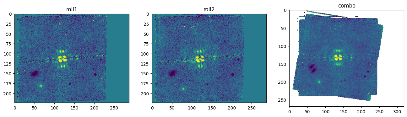
Overlay sky coordinates#
Overlay the RA and Dec grid over the combined rolls
with fits.open(i2dfiles[0]) as f:
    wcs = WCS(f[1].header)
WARNING: FITSFixedWarning: 'datfix' made the change 'Set DATE-BEG to '2022-07-17T22:58:10.204' from MJD-BEG.
Set DATE-AVG to '2022-07-18T00:15:08.760' from MJD-AVG.
Set DATE-END to '2022-07-18T01:32:07.316' from MJD-END'. [astropy.wcs.wcs]
WARNING: FITSFixedWarning: 'obsfix' made the change 'Set OBSGEO-L to   -69.981478 from OBSGEO-[XYZ].
Set OBSGEO-B to   -37.692706 from OBSGEO-[XYZ].
Set OBSGEO-H to 1737840324.368 from OBSGEO-[XYZ]'. [astropy.wcs.wcs]
# The star coordinates at the time of observation are in the header
exp_file = uncal_sci_r1_files[0]
targ_ra = fits.getval(exp_file, 'TARG_RA', 0)
targ_dec = fits.getval(exp_file, 'TARG_DEC', 0)
starcoord = SkyCoord(targ_ra, targ_dec, unit='deg', frame='icrs')
fig, ax = plt.subplots(1, 1, subplot_kw={'projection': wcs})
vmin, vmax = np.nanquantile(imgs['combo'], [0.01, 0.99])
ax.imshow(imgs['combo'], vmin=vmin, vmax=vmax)
ax.scatter(*wcs.world_to_pixel(starcoord),
           marker='x', s=100, c='w')
ax.grid(True)
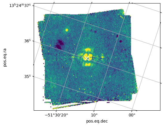
9.-Advanced Usage- PSF Reference Library#
In the above sections, we processed a single observation of a science target and its associated PSF reference target. However, the JWST archive contains many observations of MIRI coronagraphic PSF reference targets that could be used to construct a larger library of reference PSFs for improved PSF subtraction. In this section, we’ll show how to use multiple observations of different PSF reference targets through the pipeline and assemble them into a single association that can be used for PSF subtraction.
First we need to query the MAST database for potential references, and to do so we will make use of functions held within the local coron_psflib_functions.py file.
download_coron_references=None

# Check PSF library functions code is available to import
if importlib.util.find_spec("coron_psflib_functions") is None:
    print("Could not find `coron_psflib_functions.py` on the Python path or in the current project. Please ensure you have the latest pipeline notebook installation, or download `coron_psflib_functions.py` from the notebook repository directly.")
else:
    from coron_psflib_functions import download_coron_references
    print("Imported `coron_psflib_functions.py` successfully")
Imported `coron_psflib_functions.py` successfully
# If the relevant psflib functions were found and docoron3_psflib is True, proceed with PSF reference library
if download_coron_references and docoron3_psflib:
    # In this case we'll skip to the stage 2 products to avoid manual reprocessing.
    additional_ref_dir = os.path.join(basedir, 'ObsRef/stage2/')

    # We also need to provide the current calibrated science and reference files we're using so that we can match an appropriate reference and avoid duplicates.
    current_files = np.concatenate([calfiles, ref_targ_files])

    # Run function to download the files
    download_coron_references(current_files, download_dir=additional_ref_dir, num_refs=2)
Now that we have some files downloaded, we can simply add them to the reference target files list.
# Gather the filenames of the downloaded additional reference files.
if download_coron_references and docoron3_psflib:
    # Get the files
    sstring = os.path.join(additional_ref_dir, 'jw*mirimage*calints.fits')
    additional_ref_targ_files = sorted(glob.glob(sstring))

    # Add them to the current list
    psflib_ref_targ_files = np.concatenate([ref_targ_files, additional_ref_targ_files])

    # Check that these are the mask/filter to use
    psflib_ref_targ_files = select_mask_filter_files(psflib_ref_targ_files, use_mask, use_filter)
And run the Coron3 pipeline using the same settings as before using the call method.
if download_coron_references and docoron3_psflib:
    asnfile = os.path.join(coron3_psflib_dir, 'l3asn.json')
    writel3asn(calfiles, psflib_ref_targ_files, asnfile, 'Level 3')
    Coron3Pipeline.call(asnfile, steps=coron3dict, save_results=True, output_dir=coron3_psflib_dir)
else:
    print('Skipping coron3 processing')
/home/runner/micromamba/envs/ci-env/lib/python3.13/site-packages/jwst/associations/association.py:232: UserWarning: Input association file contains path information; note that this can complicate usage and/or sharing of such files.
  warnings.warn(err_str, UserWarning, stacklevel=1)
2026-04-15 20:42:59,873 - stpipe.step - INFO - PARS-RESAMPLESTEP parameters found: /home/runner/crds/references/jwst/miri/jwst_miri_pars-resamplestep_0001.asdf
2026-04-15 20:42:59,884 - stpipe.step - INFO - Coron3Pipeline instance created.
2026-04-15 20:42:59,885 - stpipe.step - INFO - StackRefsStep instance created.
2026-04-15 20:42:59,886 - stpipe.step - INFO - AlignRefsStep instance created.
2026-04-15 20:42:59,887 - stpipe.step - INFO - KlipStep instance created.
2026-04-15 20:42:59,888 - stpipe.step - INFO - OutlierDetectionStep instance created.
2026-04-15 20:42:59,889 - stpipe.step - INFO - ResampleStep instance created.
2026-04-15 20:43:00,088 - stpipe.step - INFO - Step Coron3Pipeline running with args ('./miri_coro_demo_data/stage3_psflib/l3asn.json',).
2026-04-15 20:43:00,096 - stpipe.step - INFO - Step Coron3Pipeline parameters are:
  pre_hooks: []
  post_hooks: []
  output_file: None
  output_dir: ./miri_coro_demo_data/stage3_psflib/
  output_ext: .fits
  output_use_model: False
  output_use_index: True
  save_results: True
  skip: False
  suffix: i2d
  search_output_file: True
  input_dir: ''
  steps:
    stack_refs:
      pre_hooks: []
      post_hooks: []
      output_file: None
      output_dir: None
      output_ext: .fits
      output_use_model: False
      output_use_index: True
      save_results: False
      skip: False
      suffix: None
      search_output_file: True
      input_dir: ''
    align_refs:
      pre_hooks: []
      post_hooks: []
      output_file: None
      output_dir: None
      output_ext: .fits
      output_use_model: False
      output_use_index: True
      save_results: False
      skip: False
      suffix: None
      search_output_file: True
      input_dir: ''
      median_box_length: 3
      bad_bits: DO_NOT_USE
    klip:
      pre_hooks: []
      post_hooks: []
      output_file: None
      output_dir: None
      output_ext: .fits
      output_use_model: False
      output_use_index: True
      save_results: False
      skip: False
      suffix: None
      search_output_file: True
      input_dir: ''
      truncate: 25
    outlier_detection:
      pre_hooks: []
      post_hooks: []
      output_file: None
      output_dir: None
      output_ext: .fits
      output_use_model: False
      output_use_index: True
      save_results: False
      skip: False
      suffix: None
      search_output_file: False
      input_dir: ''
      weight_type: ivm
      pixfrac: 1.0
      kernel: square
      fillval: NAN
      maskpt: 0.7
      snr: 5.0 4.0
      scale: 1.2 0.7
      backg: 0.0
      kernel_size: 7 7
      threshold_percent: 99.8
      rolling_window_width: 25
      ifu_second_check: False
      save_intermediate_results: False
      resample_data: True
      good_bits: ~DO_NOT_USE
      in_memory: True
      pixmap_stepsize: 1.0
      pixmap_order: 1
    resample:
      pre_hooks: []
      post_hooks: []
      output_file: None
      output_dir: None
      output_ext: .fits
      output_use_model: False
      output_use_index: True
      save_results: False
      skip: False
      suffix: None
      search_output_file: True
      input_dir: ''
      pixfrac: 1.0
      kernel: square
      fillval: NAN
      weight_type: exptime
      output_shape: None
      crpix: None
      crval: None
      rotation: None
      pixel_scale_ratio: 1.0
      pixel_scale: None
      output_wcs: ''
      single: False
      blendheaders: True
      in_memory: True
      enable_ctx: True
      enable_err: True
      report_var: True
      propagate_dq: False
      pixmap_stepsize: 1.0
      pixmap_order: 1
2026-04-15 20:43:00,099 - jwst.pipeline.calwebb_coron3 - INFO - Starting calwebb_coron3 ...
2026-04-15 20:43:03,343 - stpipe.pipeline - INFO - Prefetching reference files for dataset: 'jw01386007001_04101_00001_mirimage_calints.fits' reftypes = ['psfmask']
2026-04-15 20:43:03,346 - stpipe.pipeline - INFO - Prefetch for PSFMASK reference file is '/home/runner/crds/references/jwst/miri/jwst_miri_psfmask_0012.fits'.
2026-04-15 20:43:03,347 - stpipe.pipeline - INFO - Prefetching reference files for dataset: 'jw01386007001_04101_00002_mirimage_calints.fits' reftypes = ['psfmask']
2026-04-15 20:43:03,350 - stpipe.pipeline - INFO - Prefetch for PSFMASK reference file is '/home/runner/crds/references/jwst/miri/jwst_miri_psfmask_0012.fits'.
2026-04-15 20:43:03,351 - stpipe.pipeline - INFO - Prefetching reference files for dataset: 'jw01386007001_04101_00003_mirimage_calints.fits' reftypes = ['psfmask']
2026-04-15 20:43:03,353 - stpipe.pipeline - INFO - Prefetch for PSFMASK reference file is '/home/runner/crds/references/jwst/miri/jwst_miri_psfmask_0012.fits'.
2026-04-15 20:43:03,355 - stpipe.pipeline - INFO - Prefetching reference files for dataset: 'jw01386007001_04101_00004_mirimage_calints.fits' reftypes = ['psfmask']
2026-04-15 20:43:03,357 - stpipe.pipeline - INFO - Prefetch for PSFMASK reference file is '/home/runner/crds/references/jwst/miri/jwst_miri_psfmask_0012.fits'.
2026-04-15 20:43:03,359 - stpipe.pipeline - INFO - Prefetching reference files for dataset: 'jw01386007001_04101_00005_mirimage_calints.fits' reftypes = ['psfmask']
2026-04-15 20:43:03,361 - stpipe.pipeline - INFO - Prefetch for PSFMASK reference file is '/home/runner/crds/references/jwst/miri/jwst_miri_psfmask_0012.fits'.
2026-04-15 20:43:03,363 - stpipe.pipeline - INFO - Prefetching reference files for dataset: 'jw01386007001_04101_00006_mirimage_calints.fits' reftypes = ['psfmask']
2026-04-15 20:43:03,365 - stpipe.pipeline - INFO - Prefetch for PSFMASK reference file is '/home/runner/crds/references/jwst/miri/jwst_miri_psfmask_0012.fits'.
2026-04-15 20:43:03,367 - stpipe.pipeline - INFO - Prefetching reference files for dataset: 'jw01386007001_04101_00007_mirimage_calints.fits' reftypes = ['psfmask']
2026-04-15 20:43:03,369 - stpipe.pipeline - INFO - Prefetch for PSFMASK reference file is '/home/runner/crds/references/jwst/miri/jwst_miri_psfmask_0012.fits'.
2026-04-15 20:43:03,370 - stpipe.pipeline - INFO - Prefetching reference files for dataset: 'jw01386007001_04101_00008_mirimage_calints.fits' reftypes = ['psfmask']
2026-04-15 20:43:03,373 - stpipe.pipeline - INFO - Prefetch for PSFMASK reference file is '/home/runner/crds/references/jwst/miri/jwst_miri_psfmask_0012.fits'.
2026-04-15 20:43:03,374 - stpipe.pipeline - INFO - Prefetching reference files for dataset: 'jw01386007001_04101_00009_mirimage_calints.fits' reftypes = ['psfmask']
2026-04-15 20:43:03,377 - stpipe.pipeline - INFO - Prefetch for PSFMASK reference file is '/home/runner/crds/references/jwst/miri/jwst_miri_psfmask_0012.fits'.
2026-04-15 20:43:03,378 - stpipe.pipeline - INFO - Prefetching reference files for dataset: 'jw01194016001_04101_00001_mirimage_calints.fits' reftypes = ['psfmask']
2026-04-15 20:43:03,422 - stpipe.pipeline - INFO - Prefetch for PSFMASK reference file is '/home/runner/crds/references/jwst/miri/jwst_miri_psfmask_0012.fits'.
2026-04-15 20:43:03,424 - stpipe.pipeline - INFO - Prefetching reference files for dataset: 'jw01194016001_04101_00002_mirimage_calints.fits' reftypes = ['psfmask']
2026-04-15 20:43:03,426 - stpipe.pipeline - INFO - Prefetch for PSFMASK reference file is '/home/runner/crds/references/jwst/miri/jwst_miri_psfmask_0012.fits'.
2026-04-15 20:43:03,428 - stpipe.pipeline - INFO - Prefetching reference files for dataset: 'jw01194016001_04101_00003_mirimage_calints.fits' reftypes = ['psfmask']
2026-04-15 20:43:03,430 - stpipe.pipeline - INFO - Prefetch for PSFMASK reference file is '/home/runner/crds/references/jwst/miri/jwst_miri_psfmask_0012.fits'.
2026-04-15 20:43:03,431 - stpipe.pipeline - INFO - Prefetching reference files for dataset: 'jw01194016001_04101_00004_mirimage_calints.fits' reftypes = ['psfmask']
2026-04-15 20:43:03,433 - stpipe.pipeline - INFO - Prefetch for PSFMASK reference file is '/home/runner/crds/references/jwst/miri/jwst_miri_psfmask_0012.fits'.
2026-04-15 20:43:03,435 - stpipe.pipeline - INFO - Prefetching reference files for dataset: 'jw01194016001_04101_00005_mirimage_calints.fits' reftypes = ['psfmask']
2026-04-15 20:43:03,437 - stpipe.pipeline - INFO - Prefetch for PSFMASK reference file is '/home/runner/crds/references/jwst/miri/jwst_miri_psfmask_0012.fits'.
2026-04-15 20:43:03,438 - stpipe.pipeline - INFO - Prefetching reference files for dataset: 'jw01194016001_04101_00006_mirimage_calints.fits' reftypes = ['psfmask']
2026-04-15 20:43:03,441 - stpipe.pipeline - INFO - Prefetch for PSFMASK reference file is '/home/runner/crds/references/jwst/miri/jwst_miri_psfmask_0012.fits'.
2026-04-15 20:43:03,442 - stpipe.pipeline - INFO - Prefetching reference files for dataset: 'jw01194016001_04101_00007_mirimage_calints.fits' reftypes = ['psfmask']
2026-04-15 20:43:03,444 - stpipe.pipeline - INFO - Prefetch for PSFMASK reference file is '/home/runner/crds/references/jwst/miri/jwst_miri_psfmask_0012.fits'.
2026-04-15 20:43:03,446 - stpipe.pipeline - INFO - Prefetching reference files for dataset: 'jw01194016001_04101_00008_mirimage_calints.fits' reftypes = ['psfmask']
2026-04-15 20:43:03,448 - stpipe.pipeline - INFO - Prefetch for PSFMASK reference file is '/home/runner/crds/references/jwst/miri/jwst_miri_psfmask_0012.fits'.
2026-04-15 20:43:03,449 - stpipe.pipeline - INFO - Prefetching reference files for dataset: 'jw01194016001_04101_00009_mirimage_calints.fits' reftypes = ['psfmask']
2026-04-15 20:43:03,452 - stpipe.pipeline - INFO - Prefetch for PSFMASK reference file is '/home/runner/crds/references/jwst/miri/jwst_miri_psfmask_0012.fits'.
2026-04-15 20:43:03,453 - stpipe.pipeline - INFO - Prefetching reference files for dataset: 'jw01411008001_04101_00001_mirimage_calints.fits' reftypes = ['psfmask']
2026-04-15 20:43:03,455 - stpipe.pipeline - INFO - Prefetch for PSFMASK reference file is '/home/runner/crds/references/jwst/miri/jwst_miri_psfmask_0012.fits'.
2026-04-15 20:43:03,457 - stpipe.pipeline - INFO - Prefetching reference files for dataset: 'jw01411008001_04101_00002_mirimage_calints.fits' reftypes = ['psfmask']
2026-04-15 20:43:03,459 - stpipe.pipeline - INFO - Prefetch for PSFMASK reference file is '/home/runner/crds/references/jwst/miri/jwst_miri_psfmask_0012.fits'.
2026-04-15 20:43:03,460 - stpipe.pipeline - INFO - Prefetching reference files for dataset: 'jw01411008001_04101_00003_mirimage_calints.fits' reftypes = ['psfmask']
2026-04-15 20:43:03,463 - stpipe.pipeline - INFO - Prefetch for PSFMASK reference file is '/home/runner/crds/references/jwst/miri/jwst_miri_psfmask_0012.fits'.
2026-04-15 20:43:03,464 - stpipe.pipeline - INFO - Prefetching reference files for dataset: 'jw01411008001_04101_00004_mirimage_calints.fits' reftypes = ['psfmask']
2026-04-15 20:43:03,466 - stpipe.pipeline - INFO - Prefetch for PSFMASK reference file is '/home/runner/crds/references/jwst/miri/jwst_miri_psfmask_0012.fits'.
2026-04-15 20:43:03,468 - stpipe.pipeline - INFO - Prefetching reference files for dataset: 'jw01411008001_04101_00005_mirimage_calints.fits' reftypes = ['psfmask']
2026-04-15 20:43:03,470 - stpipe.pipeline - INFO - Prefetch for PSFMASK reference file is '/home/runner/crds/references/jwst/miri/jwst_miri_psfmask_0012.fits'.
2026-04-15 20:43:03,471 - stpipe.pipeline - INFO - Prefetching reference files for dataset: 'jw01386008001_04101_00001_mirimage_calints.fits' reftypes = ['psfmask']
2026-04-15 20:43:03,473 - stpipe.pipeline - INFO - Prefetch for PSFMASK reference file is '/home/runner/crds/references/jwst/miri/jwst_miri_psfmask_0012.fits'.
2026-04-15 20:43:03,475 - stpipe.pipeline - INFO - Prefetching reference files for dataset: 'jw01386009001_04101_00001_mirimage_calints.fits' reftypes = ['psfmask']
2026-04-15 20:43:03,477 - stpipe.pipeline - INFO - Prefetch for PSFMASK reference file is '/home/runner/crds/references/jwst/miri/jwst_miri_psfmask_0012.fits'.
2026-04-15 20:43:03,791 - stpipe.step - INFO - Step outlier_detection running with args (<CubeModel(19, 224, 288) from jw01386007001_04101_00001_mirimage_calints.fits>,).
2026-04-15 20:43:03,792 - jwst.outlier_detection.outlier_detection_step - INFO - Outlier Detection mode: coron
2026-04-15 20:43:03,793 - jwst.outlier_detection.outlier_detection_step - INFO - Outlier Detection asn_id: a3001
2026-04-15 20:43:03,802 - jwst.outlier_detection.utils - INFO - Computing median
2026-04-15 20:43:03,933 - jwst.outlier_detection.utils - INFO - 64 pixels marked as outliers
2026-04-15 20:43:04,052 - stpipe.step - INFO - Saved model in ./miri_coro_demo_data/stage3_psflib/jw01386007001_04101_00001_mirimage_a3001_crfints.fits
2026-04-15 20:43:04,053 - stpipe.step - INFO - Step outlier_detection done
2026-04-15 20:43:04,266 - stpipe.step - INFO - Step outlier_detection running with args (<CubeModel(19, 224, 288) from jw01386007001_04101_00002_mirimage_calints.fits>,).
2026-04-15 20:43:04,267 - jwst.outlier_detection.outlier_detection_step - INFO - Outlier Detection mode: coron
2026-04-15 20:43:04,268 - jwst.outlier_detection.outlier_detection_step - INFO - Outlier Detection asn_id: a3001
2026-04-15 20:43:04,275 - jwst.outlier_detection.utils - INFO - Computing median
2026-04-15 20:43:04,402 - jwst.outlier_detection.utils - INFO - 62 pixels marked as outliers
2026-04-15 20:43:04,521 - stpipe.step - INFO - Saved model in ./miri_coro_demo_data/stage3_psflib/jw01386007001_04101_00002_mirimage_a3001_crfints.fits
2026-04-15 20:43:04,522 - stpipe.step - INFO - Step outlier_detection done
2026-04-15 20:43:04,732 - stpipe.step - INFO - Step outlier_detection running with args (<CubeModel(19, 224, 288) from jw01386007001_04101_00003_mirimage_calints.fits>,).
2026-04-15 20:43:04,733 - jwst.outlier_detection.outlier_detection_step - INFO - Outlier Detection mode: coron
2026-04-15 20:43:04,733 - jwst.outlier_detection.outlier_detection_step - INFO - Outlier Detection asn_id: a3001
2026-04-15 20:43:04,740 - jwst.outlier_detection.utils - INFO - Computing median
2026-04-15 20:43:04,867 - jwst.outlier_detection.utils - INFO - 128 pixels marked as outliers
2026-04-15 20:43:04,988 - stpipe.step - INFO - Saved model in ./miri_coro_demo_data/stage3_psflib/jw01386007001_04101_00003_mirimage_a3001_crfints.fits
2026-04-15 20:43:04,989 - stpipe.step - INFO - Step outlier_detection done
2026-04-15 20:43:05,201 - stpipe.step - INFO - Step outlier_detection running with args (<CubeModel(19, 224, 288) from jw01386007001_04101_00004_mirimage_calints.fits>,).
2026-04-15 20:43:05,202 - jwst.outlier_detection.outlier_detection_step - INFO - Outlier Detection mode: coron
2026-04-15 20:43:05,203 - jwst.outlier_detection.outlier_detection_step - INFO - Outlier Detection asn_id: a3001
2026-04-15 20:43:05,210 - jwst.outlier_detection.utils - INFO - Computing median
2026-04-15 20:43:05,337 - jwst.outlier_detection.utils - INFO - 128 pixels marked as outliers
2026-04-15 20:43:05,457 - stpipe.step - INFO - Saved model in ./miri_coro_demo_data/stage3_psflib/jw01386007001_04101_00004_mirimage_a3001_crfints.fits
2026-04-15 20:43:05,458 - stpipe.step - INFO - Step outlier_detection done
2026-04-15 20:43:05,671 - stpipe.step - INFO - Step outlier_detection running with args (<CubeModel(19, 224, 288) from jw01386007001_04101_00005_mirimage_calints.fits>,).
2026-04-15 20:43:05,672 - jwst.outlier_detection.outlier_detection_step - INFO - Outlier Detection mode: coron
2026-04-15 20:43:05,673 - jwst.outlier_detection.outlier_detection_step - INFO - Outlier Detection asn_id: a3001
2026-04-15 20:43:05,680 - jwst.outlier_detection.utils - INFO - Computing median
2026-04-15 20:43:05,808 - jwst.outlier_detection.utils - INFO - 115 pixels marked as outliers
2026-04-15 20:43:05,928 - stpipe.step - INFO - Saved model in ./miri_coro_demo_data/stage3_psflib/jw01386007001_04101_00005_mirimage_a3001_crfints.fits
2026-04-15 20:43:05,929 - stpipe.step - INFO - Step outlier_detection done
2026-04-15 20:43:06,144 - stpipe.step - INFO - Step outlier_detection running with args (<CubeModel(19, 224, 288) from jw01386007001_04101_00006_mirimage_calints.fits>,).
2026-04-15 20:43:06,145 - jwst.outlier_detection.outlier_detection_step - INFO - Outlier Detection mode: coron
2026-04-15 20:43:06,145 - jwst.outlier_detection.outlier_detection_step - INFO - Outlier Detection asn_id: a3001
2026-04-15 20:43:06,152 - jwst.outlier_detection.utils - INFO - Computing median
2026-04-15 20:43:06,281 - jwst.outlier_detection.utils - INFO - 155 pixels marked as outliers
2026-04-15 20:43:06,401 - stpipe.step - INFO - Saved model in ./miri_coro_demo_data/stage3_psflib/jw01386007001_04101_00006_mirimage_a3001_crfints.fits
2026-04-15 20:43:06,402 - stpipe.step - INFO - Step outlier_detection done
2026-04-15 20:43:06,615 - stpipe.step - INFO - Step outlier_detection running with args (<CubeModel(19, 224, 288) from jw01386007001_04101_00007_mirimage_calints.fits>,).
2026-04-15 20:43:06,617 - jwst.outlier_detection.outlier_detection_step - INFO - Outlier Detection mode: coron
2026-04-15 20:43:06,617 - jwst.outlier_detection.outlier_detection_step - INFO - Outlier Detection asn_id: a3001
2026-04-15 20:43:06,624 - jwst.outlier_detection.utils - INFO - Computing median
2026-04-15 20:43:06,752 - jwst.outlier_detection.utils - INFO - 213 pixels marked as outliers
2026-04-15 20:43:06,873 - stpipe.step - INFO - Saved model in ./miri_coro_demo_data/stage3_psflib/jw01386007001_04101_00007_mirimage_a3001_crfints.fits
2026-04-15 20:43:06,873 - stpipe.step - INFO - Step outlier_detection done
2026-04-15 20:43:07,087 - stpipe.step - INFO - Step outlier_detection running with args (<CubeModel(19, 224, 288) from jw01386007001_04101_00008_mirimage_calints.fits>,).
2026-04-15 20:43:07,088 - jwst.outlier_detection.outlier_detection_step - INFO - Outlier Detection mode: coron
2026-04-15 20:43:07,089 - jwst.outlier_detection.outlier_detection_step - INFO - Outlier Detection asn_id: a3001
2026-04-15 20:43:07,096 - jwst.outlier_detection.utils - INFO - Computing median
2026-04-15 20:43:07,224 - jwst.outlier_detection.utils - INFO - 250 pixels marked as outliers
2026-04-15 20:43:07,346 - stpipe.step - INFO - Saved model in ./miri_coro_demo_data/stage3_psflib/jw01386007001_04101_00008_mirimage_a3001_crfints.fits
2026-04-15 20:43:07,347 - stpipe.step - INFO - Step outlier_detection done
2026-04-15 20:43:07,561 - stpipe.step - INFO - Step outlier_detection running with args (<CubeModel(19, 224, 288) from jw01386007001_04101_00009_mirimage_calints.fits>,).
2026-04-15 20:43:07,562 - jwst.outlier_detection.outlier_detection_step - INFO - Outlier Detection mode: coron
2026-04-15 20:43:07,563 - jwst.outlier_detection.outlier_detection_step - INFO - Outlier Detection asn_id: a3001
2026-04-15 20:43:07,570 - jwst.outlier_detection.utils - INFO - Computing median
2026-04-15 20:43:07,697 - jwst.outlier_detection.utils - INFO - 216 pixels marked as outliers
2026-04-15 20:43:07,818 - stpipe.step - INFO - Saved model in ./miri_coro_demo_data/stage3_psflib/jw01386007001_04101_00009_mirimage_a3001_crfints.fits
2026-04-15 20:43:07,819 - stpipe.step - INFO - Step outlier_detection done
2026-04-15 20:43:08,024 - stpipe.step - INFO - Step outlier_detection running with args (<CubeModel(2, 224, 288) from jw01194016001_04101_00001_mirimage_calints.fits>,).
2026-04-15 20:43:08,025 - jwst.outlier_detection.outlier_detection_step - INFO - Outlier Detection mode: coron
2026-04-15 20:43:08,026 - jwst.outlier_detection.outlier_detection_step - INFO - Outlier Detection asn_id: a3001
2026-04-15 20:43:08,032 - jwst.outlier_detection.utils - INFO - Computing median
2026-04-15 20:43:08,120 - jwst.outlier_detection.utils - INFO - 42 pixels marked as outliers
2026-04-15 20:43:08,222 - stpipe.step - INFO - Saved model in ./miri_coro_demo_data/stage3_psflib/jw01194016001_04101_00001_mirimage_a3001_crfints.fits
2026-04-15 20:43:08,223 - stpipe.step - INFO - Step outlier_detection done
2026-04-15 20:43:08,428 - stpipe.step - INFO - Step outlier_detection running with args (<CubeModel(2, 224, 288) from jw01194016001_04101_00002_mirimage_calints.fits>,).
2026-04-15 20:43:08,429 - jwst.outlier_detection.outlier_detection_step - INFO - Outlier Detection mode: coron
2026-04-15 20:43:08,430 - jwst.outlier_detection.outlier_detection_step - INFO - Outlier Detection asn_id: a3001
2026-04-15 20:43:08,436 - jwst.outlier_detection.utils - INFO - Computing median
2026-04-15 20:43:08,523 - jwst.outlier_detection.utils - INFO - 43 pixels marked as outliers
2026-04-15 20:43:08,625 - stpipe.step - INFO - Saved model in ./miri_coro_demo_data/stage3_psflib/jw01194016001_04101_00002_mirimage_a3001_crfints.fits
2026-04-15 20:43:08,626 - stpipe.step - INFO - Step outlier_detection done
2026-04-15 20:43:08,831 - stpipe.step - INFO - Step outlier_detection running with args (<CubeModel(2, 224, 288) from jw01194016001_04101_00003_mirimage_calints.fits>,).
2026-04-15 20:43:08,832 - jwst.outlier_detection.outlier_detection_step - INFO - Outlier Detection mode: coron
2026-04-15 20:43:08,833 - jwst.outlier_detection.outlier_detection_step - INFO - Outlier Detection asn_id: a3001
2026-04-15 20:43:08,840 - jwst.outlier_detection.utils - INFO - Computing median
2026-04-15 20:43:08,928 - jwst.outlier_detection.utils - INFO - 42 pixels marked as outliers
2026-04-15 20:43:09,030 - stpipe.step - INFO - Saved model in ./miri_coro_demo_data/stage3_psflib/jw01194016001_04101_00003_mirimage_a3001_crfints.fits
2026-04-15 20:43:09,031 - stpipe.step - INFO - Step outlier_detection done
2026-04-15 20:43:09,242 - stpipe.step - INFO - Step outlier_detection running with args (<CubeModel(2, 224, 288) from jw01194016001_04101_00004_mirimage_calints.fits>,).
2026-04-15 20:43:09,243 - jwst.outlier_detection.outlier_detection_step - INFO - Outlier Detection mode: coron
2026-04-15 20:43:09,244 - jwst.outlier_detection.outlier_detection_step - INFO - Outlier Detection asn_id: a3001
2026-04-15 20:43:09,250 - jwst.outlier_detection.utils - INFO - Computing median
2026-04-15 20:43:09,338 - jwst.outlier_detection.utils - INFO - 37 pixels marked as outliers
2026-04-15 20:43:09,441 - stpipe.step - INFO - Saved model in ./miri_coro_demo_data/stage3_psflib/jw01194016001_04101_00004_mirimage_a3001_crfints.fits
2026-04-15 20:43:09,442 - stpipe.step - INFO - Step outlier_detection done
2026-04-15 20:43:09,642 - stpipe.step - INFO - Step outlier_detection running with args (<CubeModel(2, 224, 288) from jw01194016001_04101_00005_mirimage_calints.fits>,).
2026-04-15 20:43:09,643 - jwst.outlier_detection.outlier_detection_step - INFO - Outlier Detection mode: coron
2026-04-15 20:43:09,644 - jwst.outlier_detection.outlier_detection_step - INFO - Outlier Detection asn_id: a3001
2026-04-15 20:43:09,650 - jwst.outlier_detection.utils - INFO - Computing median
2026-04-15 20:43:09,738 - jwst.outlier_detection.utils - INFO - 62 pixels marked as outliers
2026-04-15 20:43:09,843 - stpipe.step - INFO - Saved model in ./miri_coro_demo_data/stage3_psflib/jw01194016001_04101_00005_mirimage_a3001_crfints.fits
2026-04-15 20:43:09,844 - stpipe.step - INFO - Step outlier_detection done
2026-04-15 20:43:10,059 - stpipe.step - INFO - Step outlier_detection running with args (<CubeModel(2, 224, 288) from jw01194016001_04101_00006_mirimage_calints.fits>,).
2026-04-15 20:43:10,060 - jwst.outlier_detection.outlier_detection_step - INFO - Outlier Detection mode: coron
2026-04-15 20:43:10,061 - jwst.outlier_detection.outlier_detection_step - INFO - Outlier Detection asn_id: a3001
2026-04-15 20:43:10,068 - jwst.outlier_detection.utils - INFO - Computing median
2026-04-15 20:43:10,155 - jwst.outlier_detection.utils - INFO - 27 pixels marked as outliers
2026-04-15 20:43:10,260 - stpipe.step - INFO - Saved model in ./miri_coro_demo_data/stage3_psflib/jw01194016001_04101_00006_mirimage_a3001_crfints.fits
2026-04-15 20:43:10,261 - stpipe.step - INFO - Step outlier_detection done
2026-04-15 20:43:10,473 - stpipe.step - INFO - Step outlier_detection running with args (<CubeModel(2, 224, 288) from jw01194016001_04101_00007_mirimage_calints.fits>,).
2026-04-15 20:43:10,474 - jwst.outlier_detection.outlier_detection_step - INFO - Outlier Detection mode: coron
2026-04-15 20:43:10,475 - jwst.outlier_detection.outlier_detection_step - INFO - Outlier Detection asn_id: a3001
2026-04-15 20:43:10,481 - jwst.outlier_detection.utils - INFO - Computing median
2026-04-15 20:43:10,568 - jwst.outlier_detection.utils - INFO - 27 pixels marked as outliers
2026-04-15 20:43:10,671 - stpipe.step - INFO - Saved model in ./miri_coro_demo_data/stage3_psflib/jw01194016001_04101_00007_mirimage_a3001_crfints.fits
2026-04-15 20:43:10,672 - stpipe.step - INFO - Step outlier_detection done
2026-04-15 20:43:10,886 - stpipe.step - INFO - Step outlier_detection running with args (<CubeModel(2, 224, 288) from jw01194016001_04101_00008_mirimage_calints.fits>,).
2026-04-15 20:43:10,887 - jwst.outlier_detection.outlier_detection_step - INFO - Outlier Detection mode: coron
2026-04-15 20:43:10,888 - jwst.outlier_detection.outlier_detection_step - INFO - Outlier Detection asn_id: a3001
2026-04-15 20:43:10,894 - jwst.outlier_detection.utils - INFO - Computing median
2026-04-15 20:43:10,981 - jwst.outlier_detection.utils - INFO - 51 pixels marked as outliers
2026-04-15 20:43:11,085 - stpipe.step - INFO - Saved model in ./miri_coro_demo_data/stage3_psflib/jw01194016001_04101_00008_mirimage_a3001_crfints.fits
2026-04-15 20:43:11,086 - stpipe.step - INFO - Step outlier_detection done
2026-04-15 20:43:11,298 - stpipe.step - INFO - Step outlier_detection running with args (<CubeModel(2, 224, 288) from jw01194016001_04101_00009_mirimage_calints.fits>,).
2026-04-15 20:43:11,299 - jwst.outlier_detection.outlier_detection_step - INFO - Outlier Detection mode: coron
2026-04-15 20:43:11,300 - jwst.outlier_detection.outlier_detection_step - INFO - Outlier Detection asn_id: a3001
2026-04-15 20:43:11,307 - jwst.outlier_detection.utils - INFO - Computing median
2026-04-15 20:43:11,395 - jwst.outlier_detection.utils - INFO - 42 pixels marked as outliers
2026-04-15 20:43:11,499 - stpipe.step - INFO - Saved model in ./miri_coro_demo_data/stage3_psflib/jw01194016001_04101_00009_mirimage_a3001_crfints.fits
2026-04-15 20:43:11,500 - stpipe.step - INFO - Step outlier_detection done
2026-04-15 20:43:11,720 - stpipe.step - INFO - Step outlier_detection running with args (<CubeModel(30, 224, 288) from jw01411008001_04101_00001_mirimage_calints.fits>,).
2026-04-15 20:43:11,721 - jwst.outlier_detection.outlier_detection_step - INFO - Outlier Detection mode: coron
2026-04-15 20:43:11,722 - jwst.outlier_detection.outlier_detection_step - INFO - Outlier Detection asn_id: a3001
2026-04-15 20:43:11,729 - jwst.outlier_detection.utils - INFO - Computing median
2026-04-15 20:43:11,882 - jwst.outlier_detection.utils - INFO - 45 pixels marked as outliers
2026-04-15 20:43:12,014 - stpipe.step - INFO - Saved model in ./miri_coro_demo_data/stage3_psflib/jw01411008001_04101_00001_mirimage_a3001_crfints.fits
2026-04-15 20:43:12,015 - stpipe.step - INFO - Step outlier_detection done
2026-04-15 20:43:12,240 - stpipe.step - INFO - Step outlier_detection running with args (<CubeModel(30, 224, 288) from jw01411008001_04101_00002_mirimage_calints.fits>,).
2026-04-15 20:43:12,241 - jwst.outlier_detection.outlier_detection_step - INFO - Outlier Detection mode: coron
2026-04-15 20:43:12,242 - jwst.outlier_detection.outlier_detection_step - INFO - Outlier Detection asn_id: a3001
2026-04-15 20:43:12,249 - jwst.outlier_detection.utils - INFO - Computing median
2026-04-15 20:43:12,399 - jwst.outlier_detection.utils - INFO - 116 pixels marked as outliers
2026-04-15 20:43:12,532 - stpipe.step - INFO - Saved model in ./miri_coro_demo_data/stage3_psflib/jw01411008001_04101_00002_mirimage_a3001_crfints.fits
2026-04-15 20:43:12,533 - stpipe.step - INFO - Step outlier_detection done
2026-04-15 20:43:12,759 - stpipe.step - INFO - Step outlier_detection running with args (<CubeModel(30, 224, 288) from jw01411008001_04101_00003_mirimage_calints.fits>,).
2026-04-15 20:43:12,760 - jwst.outlier_detection.outlier_detection_step - INFO - Outlier Detection mode: coron
2026-04-15 20:43:12,761 - jwst.outlier_detection.outlier_detection_step - INFO - Outlier Detection asn_id: a3001
2026-04-15 20:43:12,768 - jwst.outlier_detection.utils - INFO - Computing median
2026-04-15 20:43:12,918 - jwst.outlier_detection.utils - INFO - 133 pixels marked as outliers
2026-04-15 20:43:13,051 - stpipe.step - INFO - Saved model in ./miri_coro_demo_data/stage3_psflib/jw01411008001_04101_00003_mirimage_a3001_crfints.fits
2026-04-15 20:43:13,052 - stpipe.step - INFO - Step outlier_detection done
2026-04-15 20:43:13,278 - stpipe.step - INFO - Step outlier_detection running with args (<CubeModel(30, 224, 288) from jw01411008001_04101_00004_mirimage_calints.fits>,).
2026-04-15 20:43:13,279 - jwst.outlier_detection.outlier_detection_step - INFO - Outlier Detection mode: coron
2026-04-15 20:43:13,280 - jwst.outlier_detection.outlier_detection_step - INFO - Outlier Detection asn_id: a3001
2026-04-15 20:43:13,287 - jwst.outlier_detection.utils - INFO - Computing median
2026-04-15 20:43:13,437 - jwst.outlier_detection.utils - INFO - 161 pixels marked as outliers
2026-04-15 20:43:13,571 - stpipe.step - INFO - Saved model in ./miri_coro_demo_data/stage3_psflib/jw01411008001_04101_00004_mirimage_a3001_crfints.fits
2026-04-15 20:43:13,572 - stpipe.step - INFO - Step outlier_detection done
2026-04-15 20:43:13,797 - stpipe.step - INFO - Step outlier_detection running with args (<CubeModel(30, 224, 288) from jw01411008001_04101_00005_mirimage_calints.fits>,).
2026-04-15 20:43:13,799 - jwst.outlier_detection.outlier_detection_step - INFO - Outlier Detection mode: coron
2026-04-15 20:43:13,799 - jwst.outlier_detection.outlier_detection_step - INFO - Outlier Detection asn_id: a3001
2026-04-15 20:43:13,807 - jwst.outlier_detection.utils - INFO - Computing median
2026-04-15 20:43:13,958 - jwst.outlier_detection.utils - INFO - 163 pixels marked as outliers
2026-04-15 20:43:14,091 - stpipe.step - INFO - Saved model in ./miri_coro_demo_data/stage3_psflib/jw01411008001_04101_00005_mirimage_a3001_crfints.fits
2026-04-15 20:43:14,092 - stpipe.step - INFO - Step outlier_detection done
2026-04-15 20:43:14,316 - stpipe.step - INFO - Step stack_refs running with args (<jwst.datamodels.container.ModelContainer object at 0x7f933e02e8b0>,).
2026-04-15 20:43:14,332 - jwst.coron.stack_refs - INFO - Adding psf member 1 to output stack
2026-04-15 20:43:14,336 - jwst.coron.stack_refs - INFO - Adding psf member 2 to output stack
2026-04-15 20:43:14,339 - jwst.coron.stack_refs - INFO - Adding psf member 3 to output stack
2026-04-15 20:43:14,342 - jwst.coron.stack_refs - INFO - Adding psf member 4 to output stack
2026-04-15 20:43:14,346 - jwst.coron.stack_refs - INFO - Adding psf member 5 to output stack
2026-04-15 20:43:14,348 - jwst.coron.stack_refs - INFO - Adding psf member 6 to output stack
2026-04-15 20:43:14,351 - jwst.coron.stack_refs - INFO - Adding psf member 7 to output stack
2026-04-15 20:43:14,355 - jwst.coron.stack_refs - INFO - Adding psf member 8 to output stack
2026-04-15 20:43:14,357 - jwst.coron.stack_refs - INFO - Adding psf member 9 to output stack
2026-04-15 20:43:14,360 - jwst.coron.stack_refs - INFO - Adding psf member 10 to output stack
2026-04-15 20:43:14,361 - jwst.coron.stack_refs - INFO - Adding psf member 11 to output stack
2026-04-15 20:43:14,362 - jwst.coron.stack_refs - INFO - Adding psf member 12 to output stack
2026-04-15 20:43:14,363 - jwst.coron.stack_refs - INFO - Adding psf member 13 to output stack
2026-04-15 20:43:14,364 - jwst.coron.stack_refs - INFO - Adding psf member 14 to output stack
2026-04-15 20:43:14,365 - jwst.coron.stack_refs - INFO - Adding psf member 15 to output stack
2026-04-15 20:43:14,365 - jwst.coron.stack_refs - INFO - Adding psf member 16 to output stack
2026-04-15 20:43:14,366 - jwst.coron.stack_refs - INFO - Adding psf member 17 to output stack
2026-04-15 20:43:14,367 - jwst.coron.stack_refs - INFO - Adding psf member 18 to output stack
2026-04-15 20:43:14,368 - jwst.coron.stack_refs - INFO - Adding psf member 19 to output stack
2026-04-15 20:43:14,372 - jwst.coron.stack_refs - INFO - Adding psf member 20 to output stack
2026-04-15 20:43:14,376 - jwst.coron.stack_refs - INFO - Adding psf member 21 to output stack
2026-04-15 20:43:14,380 - jwst.coron.stack_refs - INFO - Adding psf member 22 to output stack
2026-04-15 20:43:14,385 - jwst.coron.stack_refs - INFO - Adding psf member 23 to output stack
2026-04-15 20:43:14,465 - stpipe.step - INFO - Step stack_refs done
2026-04-15 20:43:14,619 - stpipe.step - INFO - Saved model in ./miri_coro_demo_data/stage3_psflib/Level 3_psfstack.fits
2026-04-15 20:43:14,848 - stpipe.step - INFO - Step outlier_detection running with args (<CubeModel(60, 224, 288) from jw01386008001_04101_00001_mirimage_calints.fits>,).
2026-04-15 20:43:14,850 - jwst.outlier_detection.outlier_detection_step - INFO - Outlier Detection mode: coron
2026-04-15 20:43:14,850 - jwst.outlier_detection.outlier_detection_step - INFO - Outlier Detection asn_id: a3001
2026-04-15 20:43:14,859 - jwst.outlier_detection.utils - INFO - Computing median
2026-04-15 20:43:15,082 - jwst.outlier_detection.utils - INFO - 34 pixels marked as outliers
2026-04-15 20:43:15,245 - stpipe.step - INFO - Saved model in ./miri_coro_demo_data/stage3_psflib/jw01386008001_04101_00001_mirimage_a3001_crfints.fits
2026-04-15 20:43:15,246 - stpipe.step - INFO - Step outlier_detection done
2026-04-15 20:43:15,474 - stpipe.step - INFO - Step align_refs running with args (<CubeModel(60, 224, 288) from jw01386008001_04101_00001_mirimage_a3001_crfints.fits>, <CubeModel(339, 224, 288) from Level 3_psfstack.fits>).
2026-04-15 20:43:15,535 - jwst.coron.align_refs_step - INFO - Using PSFMASK reference file /home/runner/crds/references/jwst/miri/jwst_miri_psfmask_0012.fits
2026-04-15 20:44:39,389 - stpipe.step - INFO - Step align_refs done
2026-04-15 20:44:39,543 - stpipe.step - INFO - Saved model in ./miri_coro_demo_data/stage3_psflib/jw01386008001_04101_00001_mirimage_a3001_psfalign.fits
2026-04-15 20:44:39,769 - stpipe.step - INFO - Step klip running with args (<CubeModel(60, 224, 288) from jw01386008001_04101_00001_mirimage_a3001_crfints.fits>, <CubeModel(339, 224, 288) from jw01386008001_04101_00001_mirimage_a3001_psfalign.fits>).
2026-04-15 20:44:39,770 - jwst.coron.klip_step - INFO - KL transform truncation = 25
2026-04-15 20:45:03,652 - stpipe.step - INFO - Step klip done
2026-04-15 20:45:03,830 - stpipe.step - INFO - Saved model in ./miri_coro_demo_data/stage3_psflib/jw01386008001_04101_00001_mirimage_a3001_psfsub.fits
2026-04-15 20:45:09,448 - stpipe.step - INFO - Step outlier_detection running with args (<CubeModel(60, 224, 288) from jw01386009001_04101_00001_mirimage_calints.fits>,).
2026-04-15 20:45:09,449 - jwst.outlier_detection.outlier_detection_step - INFO - Outlier Detection mode: coron
2026-04-15 20:45:09,450 - jwst.outlier_detection.outlier_detection_step - INFO - Outlier Detection asn_id: a3001
2026-04-15 20:45:09,458 - jwst.outlier_detection.utils - INFO - Computing median
2026-04-15 20:45:09,678 - jwst.outlier_detection.utils - INFO - 31 pixels marked as outliers
2026-04-15 20:45:09,840 - stpipe.step - INFO - Saved model in ./miri_coro_demo_data/stage3_psflib/jw01386009001_04101_00001_mirimage_a3001_crfints.fits
2026-04-15 20:45:09,841 - stpipe.step - INFO - Step outlier_detection done
2026-04-15 20:45:10,065 - stpipe.step - INFO - Step align_refs running with args (<CubeModel(60, 224, 288) from jw01386009001_04101_00001_mirimage_a3001_crfints.fits>, <CubeModel(339, 224, 288) from Level 3_psfstack.fits>).
2026-04-15 20:45:10,077 - jwst.coron.align_refs_step - INFO - Using PSFMASK reference file /home/runner/crds/references/jwst/miri/jwst_miri_psfmask_0012.fits
2026-04-15 20:46:36,265 - stpipe.step - INFO - Step align_refs done
2026-04-15 20:46:36,421 - stpipe.step - INFO - Saved model in ./miri_coro_demo_data/stage3_psflib/jw01386009001_04101_00001_mirimage_a3001_psfalign.fits
2026-04-15 20:46:36,651 - stpipe.step - INFO - Step klip running with args (<CubeModel(60, 224, 288) from jw01386009001_04101_00001_mirimage_a3001_crfints.fits>, <CubeModel(339, 224, 288) from jw01386009001_04101_00001_mirimage_a3001_psfalign.fits>).
2026-04-15 20:46:36,653 - jwst.coron.klip_step - INFO - KL transform truncation = 25
2026-04-15 20:47:00,597 - stpipe.step - INFO - Step klip done
2026-04-15 20:47:00,768 - stpipe.step - INFO - Saved model in ./miri_coro_demo_data/stage3_psflib/jw01386009001_04101_00001_mirimage_a3001_psfsub.fits
2026-04-15 20:47:06,723 - stpipe.step - INFO - Step resample running with args (<jwst.datamodels.library.ModelLibrary object at 0x7f933ae583b0>,).
2026-04-15 20:47:06,927 - jwst.resample.resample_utils - INFO - Pixel scale ratio (pscale_out/pscale_in): 1.0
2026-04-15 20:47:06,928 - jwst.resample.resample_utils - INFO - Computed output pixel scale: 0.11052294295742446 arcsec.
2026-04-15 20:47:07,101 - stcal.resample.resample - INFO - Output pixel scale: 0.11052294295742446 arcsec.
2026-04-15 20:47:07,102 - stcal.resample.resample - INFO - Driz parameter kernel: square
2026-04-15 20:47:07,103 - stcal.resample.resample - INFO - Driz parameter pixfrac: 1.0
2026-04-15 20:47:07,104 - stcal.resample.resample - INFO - Driz parameter fillval: NAN
2026-04-15 20:47:07,104 - stcal.resample.resample - INFO - Driz parameter weight_type: exptime
2026-04-15 20:47:07,106 - jwst.resample.resample - INFO - Resampling science and variance data
2026-04-15 20:47:07,132 - stcal.resample.resample - INFO - Resampling science and variance data
2026-04-15 20:47:07,142 - stcal.resample.resample - INFO - Drizzling (224, 288) --> (269, 319)
2026-04-15 20:47:07,151 - stcal.resample.resample - INFO - Drizzling (224, 288) --> (269, 319)
2026-04-15 20:47:07,160 - stcal.resample.resample - INFO - Drizzling (224, 288) --> (269, 319)
2026-04-15 20:47:07,236 - stcal.resample.resample - INFO - Resampling science and variance data
2026-04-15 20:47:07,246 - stcal.resample.resample - INFO - Drizzling (224, 288) --> (269, 319)
2026-04-15 20:47:07,255 - stcal.resample.resample - INFO - Drizzling (224, 288) --> (269, 319)
2026-04-15 20:47:07,264 - stcal.resample.resample - INFO - Drizzling (224, 288) --> (269, 319)
2026-04-15 20:47:07,301 - stcal.resample.resample - INFO - Resampling science and variance data
2026-04-15 20:47:07,311 - stcal.resample.resample - INFO - Drizzling (224, 288) --> (269, 319)
2026-04-15 20:47:07,320 - stcal.resample.resample - INFO - Drizzling (224, 288) --> (269, 319)
2026-04-15 20:47:07,329 - stcal.resample.resample - INFO - Drizzling (224, 288) --> (269, 319)
2026-04-15 20:47:07,367 - stcal.resample.resample - INFO - Resampling science and variance data
2026-04-15 20:47:07,376 - stcal.resample.resample - INFO - Drizzling (224, 288) --> (269, 319)
2026-04-15 20:47:07,385 - stcal.resample.resample - INFO - Drizzling (224, 288) --> (269, 319)
2026-04-15 20:47:07,394 - stcal.resample.resample - INFO - Drizzling (224, 288) --> (269, 319)
2026-04-15 20:47:07,431 - stcal.resample.resample - INFO - Resampling science and variance data
2026-04-15 20:47:07,441 - stcal.resample.resample - INFO - Drizzling (224, 288) --> (269, 319)
2026-04-15 20:47:07,450 - stcal.resample.resample - INFO - Drizzling (224, 288) --> (269, 319)
2026-04-15 20:47:07,459 - stcal.resample.resample - INFO - Drizzling (224, 288) --> (269, 319)
2026-04-15 20:47:07,496 - stcal.resample.resample - INFO - Resampling science and variance data
2026-04-15 20:47:07,505 - stcal.resample.resample - INFO - Drizzling (224, 288) --> (269, 319)
2026-04-15 20:47:07,514 - stcal.resample.resample - INFO - Drizzling (224, 288) --> (269, 319)
2026-04-15 20:47:07,524 - stcal.resample.resample - INFO - Drizzling (224, 288) --> (269, 319)
2026-04-15 20:47:07,563 - stcal.resample.resample - INFO - Resampling science and variance data
2026-04-15 20:47:07,572 - stcal.resample.resample - INFO - Drizzling (224, 288) --> (269, 319)
2026-04-15 20:47:07,581 - stcal.resample.resample - INFO - Drizzling (224, 288) --> (269, 319)
2026-04-15 20:47:07,590 - stcal.resample.resample - INFO - Drizzling (224, 288) --> (269, 319)
2026-04-15 20:47:07,627 - stcal.resample.resample - INFO - Resampling science and variance data
2026-04-15 20:47:07,636 - stcal.resample.resample - INFO - Drizzling (224, 288) --> (269, 319)
2026-04-15 20:47:07,645 - stcal.resample.resample - INFO - Drizzling (224, 288) --> (269, 319)
2026-04-15 20:47:07,654 - stcal.resample.resample - INFO - Drizzling (224, 288) --> (269, 319)
2026-04-15 20:47:07,691 - stcal.resample.resample - INFO - Resampling science and variance data
2026-04-15 20:47:07,700 - stcal.resample.resample - INFO - Drizzling (224, 288) --> (269, 319)
2026-04-15 20:47:07,710 - stcal.resample.resample - INFO - Drizzling (224, 288) --> (269, 319)
2026-04-15 20:47:07,719 - stcal.resample.resample - INFO - Drizzling (224, 288) --> (269, 319)
2026-04-15 20:47:07,757 - stcal.resample.resample - INFO - Resampling science and variance data
2026-04-15 20:47:07,767 - stcal.resample.resample - INFO - Drizzling (224, 288) --> (269, 319)
2026-04-15 20:47:07,778 - stcal.resample.resample - INFO - Drizzling (224, 288) --> (269, 319)
2026-04-15 20:47:07,786 - stcal.resample.resample - INFO - Drizzling (224, 288) --> (269, 319)
2026-04-15 20:47:07,824 - stcal.resample.resample - INFO - Resampling science and variance data
2026-04-15 20:47:07,833 - stcal.resample.resample - INFO - Drizzling (224, 288) --> (269, 319)
2026-04-15 20:47:07,842 - stcal.resample.resample - INFO - Drizzling (224, 288) --> (269, 319)
2026-04-15 20:47:07,851 - stcal.resample.resample - INFO - Drizzling (224, 288) --> (269, 319)
2026-04-15 20:47:07,887 - stcal.resample.resample - INFO - Resampling science and variance data
2026-04-15 20:47:07,897 - stcal.resample.resample - INFO - Drizzling (224, 288) --> (269, 319)
2026-04-15 20:47:07,905 - stcal.resample.resample - INFO - Drizzling (224, 288) --> (269, 319)
2026-04-15 20:47:07,914 - stcal.resample.resample - INFO - Drizzling (224, 288) --> (269, 319)
2026-04-15 20:47:07,951 - stcal.resample.resample - INFO - Resampling science and variance data
2026-04-15 20:47:07,961 - stcal.resample.resample - INFO - Drizzling (224, 288) --> (269, 319)
2026-04-15 20:47:07,969 - stcal.resample.resample - INFO - Drizzling (224, 288) --> (269, 319)
2026-04-15 20:47:07,978 - stcal.resample.resample - INFO - Drizzling (224, 288) --> (269, 319)
2026-04-15 20:47:08,015 - stcal.resample.resample - INFO - Resampling science and variance data
2026-04-15 20:47:08,024 - stcal.resample.resample - INFO - Drizzling (224, 288) --> (269, 319)
2026-04-15 20:47:08,033 - stcal.resample.resample - INFO - Drizzling (224, 288) --> (269, 319)
2026-04-15 20:47:08,041 - stcal.resample.resample - INFO - Drizzling (224, 288) --> (269, 319)
2026-04-15 20:47:08,078 - stcal.resample.resample - INFO - Resampling science and variance data
2026-04-15 20:47:08,087 - stcal.resample.resample - INFO - Drizzling (224, 288) --> (269, 319)
2026-04-15 20:47:08,096 - stcal.resample.resample - INFO - Drizzling (224, 288) --> (269, 319)
2026-04-15 20:47:08,105 - stcal.resample.resample - INFO - Drizzling (224, 288) --> (269, 319)
2026-04-15 20:47:08,142 - stcal.resample.resample - INFO - Resampling science and variance data
2026-04-15 20:47:08,151 - stcal.resample.resample - INFO - Drizzling (224, 288) --> (269, 319)
2026-04-15 20:47:08,160 - stcal.resample.resample - INFO - Drizzling (224, 288) --> (269, 319)
2026-04-15 20:47:08,169 - stcal.resample.resample - INFO - Drizzling (224, 288) --> (269, 319)
2026-04-15 20:47:08,205 - stcal.resample.resample - INFO - Resampling science and variance data
2026-04-15 20:47:08,214 - stcal.resample.resample - INFO - Drizzling (224, 288) --> (269, 319)
2026-04-15 20:47:08,223 - stcal.resample.resample - INFO - Drizzling (224, 288) --> (269, 319)
2026-04-15 20:47:08,232 - stcal.resample.resample - INFO - Drizzling (224, 288) --> (269, 319)
2026-04-15 20:47:08,268 - stcal.resample.resample - INFO - Resampling science and variance data
2026-04-15 20:47:08,278 - stcal.resample.resample - INFO - Drizzling (224, 288) --> (269, 319)
2026-04-15 20:47:08,286 - stcal.resample.resample - INFO - Drizzling (224, 288) --> (269, 319)
2026-04-15 20:47:08,295 - stcal.resample.resample - INFO - Drizzling (224, 288) --> (269, 319)
2026-04-15 20:47:08,332 - stcal.resample.resample - INFO - Resampling science and variance data
2026-04-15 20:47:08,342 - stcal.resample.resample - INFO - Drizzling (224, 288) --> (269, 319)
2026-04-15 20:47:08,350 - stcal.resample.resample - INFO - Drizzling (224, 288) --> (269, 319)
2026-04-15 20:47:08,359 - stcal.resample.resample - INFO - Drizzling (224, 288) --> (269, 319)
2026-04-15 20:47:08,395 - stcal.resample.resample - INFO - Resampling science and variance data
2026-04-15 20:47:08,405 - stcal.resample.resample - INFO - Drizzling (224, 288) --> (269, 319)
2026-04-15 20:47:08,413 - stcal.resample.resample - INFO - Drizzling (224, 288) --> (269, 319)
2026-04-15 20:47:08,422 - stcal.resample.resample - INFO - Drizzling (224, 288) --> (269, 319)
2026-04-15 20:47:08,459 - stcal.resample.resample - INFO - Resampling science and variance data
2026-04-15 20:47:08,468 - stcal.resample.resample - INFO - Drizzling (224, 288) --> (269, 319)
2026-04-15 20:47:08,477 - stcal.resample.resample - INFO - Drizzling (224, 288) --> (269, 319)
2026-04-15 20:47:08,485 - stcal.resample.resample - INFO - Drizzling (224, 288) --> (269, 319)
2026-04-15 20:47:08,522 - stcal.resample.resample - INFO - Resampling science and variance data
2026-04-15 20:47:08,531 - stcal.resample.resample - INFO - Drizzling (224, 288) --> (269, 319)
2026-04-15 20:47:08,540 - stcal.resample.resample - INFO - Drizzling (224, 288) --> (269, 319)
2026-04-15 20:47:08,549 - stcal.resample.resample - INFO - Drizzling (224, 288) --> (269, 319)
2026-04-15 20:47:08,585 - stcal.resample.resample - INFO - Resampling science and variance data
2026-04-15 20:47:08,594 - stcal.resample.resample - INFO - Drizzling (224, 288) --> (269, 319)
2026-04-15 20:47:08,603 - stcal.resample.resample - INFO - Drizzling (224, 288) --> (269, 319)
2026-04-15 20:47:08,612 - stcal.resample.resample - INFO - Drizzling (224, 288) --> (269, 319)
2026-04-15 20:47:08,648 - stcal.resample.resample - INFO - Resampling science and variance data
2026-04-15 20:47:08,657 - stcal.resample.resample - INFO - Drizzling (224, 288) --> (269, 319)
2026-04-15 20:47:08,666 - stcal.resample.resample - INFO - Drizzling (224, 288) --> (269, 319)
2026-04-15 20:47:08,675 - stcal.resample.resample - INFO - Drizzling (224, 288) --> (269, 319)
2026-04-15 20:47:08,714 - stcal.resample.resample - INFO - Resampling science and variance data
2026-04-15 20:47:08,723 - stcal.resample.resample - INFO - Drizzling (224, 288) --> (269, 319)
2026-04-15 20:47:08,732 - stcal.resample.resample - INFO - Drizzling (224, 288) --> (269, 319)
2026-04-15 20:47:08,741 - stcal.resample.resample - INFO - Drizzling (224, 288) --> (269, 319)
2026-04-15 20:47:08,777 - stcal.resample.resample - INFO - Resampling science and variance data
2026-04-15 20:47:08,786 - stcal.resample.resample - INFO - Drizzling (224, 288) --> (269, 319)
2026-04-15 20:47:08,795 - stcal.resample.resample - INFO - Drizzling (224, 288) --> (269, 319)
2026-04-15 20:47:08,804 - stcal.resample.resample - INFO - Drizzling (224, 288) --> (269, 319)
2026-04-15 20:47:08,841 - stcal.resample.resample - INFO - Resampling science and variance data
2026-04-15 20:47:08,850 - stcal.resample.resample - INFO - Drizzling (224, 288) --> (269, 319)
2026-04-15 20:47:08,859 - stcal.resample.resample - INFO - Drizzling (224, 288) --> (269, 319)
2026-04-15 20:47:08,868 - stcal.resample.resample - INFO - Drizzling (224, 288) --> (269, 319)
2026-04-15 20:47:08,905 - stcal.resample.resample - INFO - Resampling science and variance data
2026-04-15 20:47:08,915 - stcal.resample.resample - INFO - Drizzling (224, 288) --> (269, 319)
2026-04-15 20:47:08,924 - stcal.resample.resample - INFO - Drizzling (224, 288) --> (269, 319)
2026-04-15 20:47:08,932 - stcal.resample.resample - INFO - Drizzling (224, 288) --> (269, 319)
2026-04-15 20:47:08,969 - stcal.resample.resample - INFO - Resampling science and variance data
2026-04-15 20:47:08,978 - stcal.resample.resample - INFO - Drizzling (224, 288) --> (269, 319)
2026-04-15 20:47:08,987 - stcal.resample.resample - INFO - Drizzling (224, 288) --> (269, 319)
2026-04-15 20:47:08,996 - stcal.resample.resample - INFO - Drizzling (224, 288) --> (269, 319)
2026-04-15 20:47:09,033 - stcal.resample.resample - INFO - Resampling science and variance data
2026-04-15 20:47:09,043 - stcal.resample.resample - INFO - Drizzling (224, 288) --> (269, 319)
2026-04-15 20:47:09,051 - stcal.resample.resample - INFO - Drizzling (224, 288) --> (269, 319)
2026-04-15 20:47:09,060 - stcal.resample.resample - INFO - Drizzling (224, 288) --> (269, 319)
2026-04-15 20:47:09,097 - stcal.resample.resample - INFO - Resampling science and variance data
2026-04-15 20:47:09,106 - stcal.resample.resample - INFO - Drizzling (224, 288) --> (269, 319)
2026-04-15 20:47:09,115 - stcal.resample.resample - INFO - Drizzling (224, 288) --> (269, 319)
2026-04-15 20:47:09,124 - stcal.resample.resample - INFO - Drizzling (224, 288) --> (269, 319)
2026-04-15 20:47:09,161 - stcal.resample.resample - INFO - Resampling science and variance data
2026-04-15 20:47:09,170 - stcal.resample.resample - INFO - Drizzling (224, 288) --> (269, 319)
2026-04-15 20:47:09,179 - stcal.resample.resample - INFO - Drizzling (224, 288) --> (269, 319)
2026-04-15 20:47:09,188 - stcal.resample.resample - INFO - Drizzling (224, 288) --> (269, 319)
2026-04-15 20:47:09,225 - stcal.resample.resample - INFO - Resampling science and variance data
2026-04-15 20:47:09,234 - stcal.resample.resample - INFO - Drizzling (224, 288) --> (269, 319)
2026-04-15 20:47:09,243 - stcal.resample.resample - INFO - Drizzling (224, 288) --> (269, 319)
2026-04-15 20:47:09,252 - stcal.resample.resample - INFO - Drizzling (224, 288) --> (269, 319)
2026-04-15 20:47:09,288 - stcal.resample.resample - INFO - Resampling science and variance data
2026-04-15 20:47:09,297 - stcal.resample.resample - INFO - Drizzling (224, 288) --> (269, 319)
2026-04-15 20:47:09,306 - stcal.resample.resample - INFO - Drizzling (224, 288) --> (269, 319)
2026-04-15 20:47:09,315 - stcal.resample.resample - INFO - Drizzling (224, 288) --> (269, 319)
2026-04-15 20:47:09,351 - stcal.resample.resample - INFO - Resampling science and variance data
2026-04-15 20:47:09,361 - stcal.resample.resample - INFO - Drizzling (224, 288) --> (269, 319)
2026-04-15 20:47:09,369 - stcal.resample.resample - INFO - Drizzling (224, 288) --> (269, 319)
2026-04-15 20:47:09,378 - stcal.resample.resample - INFO - Drizzling (224, 288) --> (269, 319)
2026-04-15 20:47:09,415 - stcal.resample.resample - INFO - Resampling science and variance data
2026-04-15 20:47:09,424 - stcal.resample.resample - INFO - Drizzling (224, 288) --> (269, 319)
2026-04-15 20:47:09,433 - stcal.resample.resample - INFO - Drizzling (224, 288) --> (269, 319)
2026-04-15 20:47:09,442 - stcal.resample.resample - INFO - Drizzling (224, 288) --> (269, 319)
2026-04-15 20:47:09,479 - stcal.resample.resample - INFO - Resampling science and variance data
2026-04-15 20:47:09,488 - stcal.resample.resample - INFO - Drizzling (224, 288) --> (269, 319)
2026-04-15 20:47:09,497 - stcal.resample.resample - INFO - Drizzling (224, 288) --> (269, 319)
2026-04-15 20:47:09,506 - stcal.resample.resample - INFO - Drizzling (224, 288) --> (269, 319)
2026-04-15 20:47:09,542 - stcal.resample.resample - INFO - Resampling science and variance data
2026-04-15 20:47:09,552 - stcal.resample.resample - INFO - Drizzling (224, 288) --> (269, 319)
2026-04-15 20:47:09,561 - stcal.resample.resample - INFO - Drizzling (224, 288) --> (269, 319)
2026-04-15 20:47:09,570 - stcal.resample.resample - INFO - Drizzling (224, 288) --> (269, 319)
2026-04-15 20:47:09,607 - stcal.resample.resample - INFO - Resampling science and variance data
2026-04-15 20:47:09,617 - stcal.resample.resample - INFO - Drizzling (224, 288) --> (269, 319)
2026-04-15 20:47:09,626 - stcal.resample.resample - INFO - Drizzling (224, 288) --> (269, 319)
2026-04-15 20:47:09,635 - stcal.resample.resample - INFO - Drizzling (224, 288) --> (269, 319)
2026-04-15 20:47:09,673 - stcal.resample.resample - INFO - Resampling science and variance data
2026-04-15 20:47:09,683 - stcal.resample.resample - INFO - Drizzling (224, 288) --> (269, 319)
2026-04-15 20:47:09,692 - stcal.resample.resample - INFO - Drizzling (224, 288) --> (269, 319)
2026-04-15 20:47:09,701 - stcal.resample.resample - INFO - Drizzling (224, 288) --> (269, 319)
2026-04-15 20:47:09,739 - stcal.resample.resample - INFO - Resampling science and variance data
2026-04-15 20:47:09,748 - stcal.resample.resample - INFO - Drizzling (224, 288) --> (269, 319)
2026-04-15 20:47:09,757 - stcal.resample.resample - INFO - Drizzling (224, 288) --> (269, 319)
2026-04-15 20:47:09,766 - stcal.resample.resample - INFO - Drizzling (224, 288) --> (269, 319)
2026-04-15 20:47:09,804 - stcal.resample.resample - INFO - Resampling science and variance data
2026-04-15 20:47:09,813 - stcal.resample.resample - INFO - Drizzling (224, 288) --> (269, 319)
2026-04-15 20:47:09,822 - stcal.resample.resample - INFO - Drizzling (224, 288) --> (269, 319)
2026-04-15 20:47:09,831 - stcal.resample.resample - INFO - Drizzling (224, 288) --> (269, 319)
2026-04-15 20:47:09,868 - stcal.resample.resample - INFO - Resampling science and variance data
2026-04-15 20:47:09,877 - stcal.resample.resample - INFO - Drizzling (224, 288) --> (269, 319)
2026-04-15 20:47:09,886 - stcal.resample.resample - INFO - Drizzling (224, 288) --> (269, 319)
2026-04-15 20:47:09,896 - stcal.resample.resample - INFO - Drizzling (224, 288) --> (269, 319)
2026-04-15 20:47:09,932 - stcal.resample.resample - INFO - Resampling science and variance data
2026-04-15 20:47:09,941 - stcal.resample.resample - INFO - Drizzling (224, 288) --> (269, 319)
2026-04-15 20:47:09,950 - stcal.resample.resample - INFO - Drizzling (224, 288) --> (269, 319)
2026-04-15 20:47:09,959 - stcal.resample.resample - INFO - Drizzling (224, 288) --> (269, 319)
2026-04-15 20:47:09,997 - stcal.resample.resample - INFO - Resampling science and variance data
2026-04-15 20:47:10,006 - stcal.resample.resample - INFO - Drizzling (224, 288) --> (269, 319)
2026-04-15 20:47:10,015 - stcal.resample.resample - INFO - Drizzling (224, 288) --> (269, 319)
2026-04-15 20:47:10,025 - stcal.resample.resample - INFO - Drizzling (224, 288) --> (269, 319)
2026-04-15 20:47:10,062 - stcal.resample.resample - INFO - Resampling science and variance data
2026-04-15 20:47:10,071 - stcal.resample.resample - INFO - Drizzling (224, 288) --> (269, 319)
2026-04-15 20:47:10,080 - stcal.resample.resample - INFO - Drizzling (224, 288) --> (269, 319)
2026-04-15 20:47:10,089 - stcal.resample.resample - INFO - Drizzling (224, 288) --> (269, 319)
2026-04-15 20:47:10,125 - stcal.resample.resample - INFO - Resampling science and variance data
2026-04-15 20:47:10,135 - stcal.resample.resample - INFO - Drizzling (224, 288) --> (269, 319)
2026-04-15 20:47:10,144 - stcal.resample.resample - INFO - Drizzling (224, 288) --> (269, 319)
2026-04-15 20:47:10,153 - stcal.resample.resample - INFO - Drizzling (224, 288) --> (269, 319)
2026-04-15 20:47:10,190 - stcal.resample.resample - INFO - Resampling science and variance data
2026-04-15 20:47:10,200 - stcal.resample.resample - INFO - Drizzling (224, 288) --> (269, 319)
2026-04-15 20:47:10,209 - stcal.resample.resample - INFO - Drizzling (224, 288) --> (269, 319)
2026-04-15 20:47:10,218 - stcal.resample.resample - INFO - Drizzling (224, 288) --> (269, 319)
2026-04-15 20:47:10,255 - stcal.resample.resample - INFO - Resampling science and variance data
2026-04-15 20:47:10,264 - stcal.resample.resample - INFO - Drizzling (224, 288) --> (269, 319)
2026-04-15 20:47:10,273 - stcal.resample.resample - INFO - Drizzling (224, 288) --> (269, 319)
2026-04-15 20:47:10,282 - stcal.resample.resample - INFO - Drizzling (224, 288) --> (269, 319)
2026-04-15 20:47:10,318 - stcal.resample.resample - INFO - Resampling science and variance data
2026-04-15 20:47:10,328 - stcal.resample.resample - INFO - Drizzling (224, 288) --> (269, 319)
2026-04-15 20:47:10,338 - stcal.resample.resample - INFO - Drizzling (224, 288) --> (269, 319)
2026-04-15 20:47:10,347 - stcal.resample.resample - INFO - Drizzling (224, 288) --> (269, 319)
2026-04-15 20:47:10,386 - stcal.resample.resample - INFO - Resampling science and variance data
2026-04-15 20:47:10,396 - stcal.resample.resample - INFO - Drizzling (224, 288) --> (269, 319)
2026-04-15 20:47:10,405 - stcal.resample.resample - INFO - Drizzling (224, 288) --> (269, 319)
2026-04-15 20:47:10,414 - stcal.resample.resample - INFO - Drizzling (224, 288) --> (269, 319)
2026-04-15 20:47:10,450 - stcal.resample.resample - INFO - Resampling science and variance data
2026-04-15 20:47:10,459 - stcal.resample.resample - INFO - Drizzling (224, 288) --> (269, 319)
2026-04-15 20:47:10,468 - stcal.resample.resample - INFO - Drizzling (224, 288) --> (269, 319)
2026-04-15 20:47:10,477 - stcal.resample.resample - INFO - Drizzling (224, 288) --> (269, 319)
2026-04-15 20:47:10,513 - stcal.resample.resample - INFO - Resampling science and variance data
2026-04-15 20:47:10,522 - stcal.resample.resample - INFO - Drizzling (224, 288) --> (269, 319)
2026-04-15 20:47:10,531 - stcal.resample.resample - INFO - Drizzling (224, 288) --> (269, 319)
2026-04-15 20:47:10,540 - stcal.resample.resample - INFO - Drizzling (224, 288) --> (269, 319)
2026-04-15 20:47:10,577 - stcal.resample.resample - INFO - Resampling science and variance data
2026-04-15 20:47:10,586 - stcal.resample.resample - INFO - Drizzling (224, 288) --> (269, 319)
2026-04-15 20:47:10,595 - stcal.resample.resample - INFO - Drizzling (224, 288) --> (269, 319)
2026-04-15 20:47:10,604 - stcal.resample.resample - INFO - Drizzling (224, 288) --> (269, 319)
2026-04-15 20:47:10,640 - stcal.resample.resample - INFO - Resampling science and variance data
2026-04-15 20:47:10,649 - stcal.resample.resample - INFO - Drizzling (224, 288) --> (269, 319)
2026-04-15 20:47:10,658 - stcal.resample.resample - INFO - Drizzling (224, 288) --> (269, 319)
2026-04-15 20:47:10,667 - stcal.resample.resample - INFO - Drizzling (224, 288) --> (269, 319)
2026-04-15 20:47:10,703 - stcal.resample.resample - INFO - Resampling science and variance data
2026-04-15 20:47:10,712 - stcal.resample.resample - INFO - Drizzling (224, 288) --> (269, 319)
2026-04-15 20:47:10,721 - stcal.resample.resample - INFO - Drizzling (224, 288) --> (269, 319)
2026-04-15 20:47:10,729 - stcal.resample.resample - INFO - Drizzling (224, 288) --> (269, 319)
2026-04-15 20:47:10,766 - stcal.resample.resample - INFO - Resampling science and variance data
2026-04-15 20:47:10,775 - stcal.resample.resample - INFO - Drizzling (224, 288) --> (269, 319)
2026-04-15 20:47:10,784 - stcal.resample.resample - INFO - Drizzling (224, 288) --> (269, 319)
2026-04-15 20:47:10,793 - stcal.resample.resample - INFO - Drizzling (224, 288) --> (269, 319)
2026-04-15 20:47:10,829 - stcal.resample.resample - INFO - Resampling science and variance data
2026-04-15 20:47:10,838 - stcal.resample.resample - INFO - Drizzling (224, 288) --> (269, 319)
2026-04-15 20:47:10,847 - stcal.resample.resample - INFO - Drizzling (224, 288) --> (269, 319)
2026-04-15 20:47:10,856 - stcal.resample.resample - INFO - Drizzling (224, 288) --> (269, 319)
2026-04-15 20:47:10,892 - stcal.resample.resample - INFO - Resampling science and variance data
2026-04-15 20:47:10,901 - stcal.resample.resample - INFO - Drizzling (224, 288) --> (269, 319)
2026-04-15 20:47:10,910 - stcal.resample.resample - INFO - Drizzling (224, 288) --> (269, 319)
2026-04-15 20:47:10,918 - stcal.resample.resample - INFO - Drizzling (224, 288) --> (269, 319)
2026-04-15 20:47:10,956 - stcal.resample.resample - INFO - Resampling science and variance data
2026-04-15 20:47:10,965 - stcal.resample.resample - INFO - Drizzling (224, 288) --> (269, 319)
2026-04-15 20:47:10,974 - stcal.resample.resample - INFO - Drizzling (224, 288) --> (269, 319)
2026-04-15 20:47:10,983 - stcal.resample.resample - INFO - Drizzling (224, 288) --> (269, 319)
2026-04-15 20:47:11,019 - stcal.resample.resample - INFO - Resampling science and variance data
2026-04-15 20:47:11,030 - stcal.resample.resample - INFO - Drizzling (224, 288) --> (269, 319)
2026-04-15 20:47:11,040 - stcal.resample.resample - INFO - Drizzling (224, 288) --> (269, 319)
2026-04-15 20:47:11,050 - stcal.resample.resample - INFO - Drizzling (224, 288) --> (269, 319)
2026-04-15 20:47:11,088 - stcal.resample.resample - INFO - Resampling science and variance data
2026-04-15 20:47:11,099 - stcal.resample.resample - INFO - Drizzling (224, 288) --> (269, 319)
2026-04-15 20:47:11,109 - stcal.resample.resample - INFO - Drizzling (224, 288) --> (269, 319)
2026-04-15 20:47:11,119 - stcal.resample.resample - INFO - Drizzling (224, 288) --> (269, 319)
2026-04-15 20:47:11,157 - stcal.resample.resample - INFO - Resampling science and variance data
2026-04-15 20:47:11,168 - stcal.resample.resample - INFO - Drizzling (224, 288) --> (269, 319)
2026-04-15 20:47:11,178 - stcal.resample.resample - INFO - Drizzling (224, 288) --> (269, 319)
2026-04-15 20:47:11,188 - stcal.resample.resample - INFO - Drizzling (224, 288) --> (269, 319)
2026-04-15 20:47:11,225 - stcal.resample.resample - INFO - Resampling science and variance data
2026-04-15 20:47:11,236 - stcal.resample.resample - INFO - Drizzling (224, 288) --> (269, 319)
2026-04-15 20:47:11,246 - stcal.resample.resample - INFO - Drizzling (224, 288) --> (269, 319)
2026-04-15 20:47:11,256 - stcal.resample.resample - INFO - Drizzling (224, 288) --> (269, 319)
2026-04-15 20:47:11,294 - stcal.resample.resample - INFO - Resampling science and variance data
2026-04-15 20:47:11,305 - stcal.resample.resample - INFO - Drizzling (224, 288) --> (269, 319)
2026-04-15 20:47:11,315 - stcal.resample.resample - INFO - Drizzling (224, 288) --> (269, 319)
2026-04-15 20:47:11,325 - stcal.resample.resample - INFO - Drizzling (224, 288) --> (269, 319)
2026-04-15 20:47:11,362 - stcal.resample.resample - INFO - Resampling science and variance data
2026-04-15 20:47:11,373 - stcal.resample.resample - INFO - Drizzling (224, 288) --> (269, 319)
2026-04-15 20:47:11,383 - stcal.resample.resample - INFO - Drizzling (224, 288) --> (269, 319)
2026-04-15 20:47:11,392 - stcal.resample.resample - INFO - Drizzling (224, 288) --> (269, 319)
2026-04-15 20:47:11,430 - stcal.resample.resample - INFO - Resampling science and variance data
2026-04-15 20:47:11,440 - stcal.resample.resample - INFO - Drizzling (224, 288) --> (269, 319)
2026-04-15 20:47:11,450 - stcal.resample.resample - INFO - Drizzling (224, 288) --> (269, 319)
2026-04-15 20:47:11,460 - stcal.resample.resample - INFO - Drizzling (224, 288) --> (269, 319)
2026-04-15 20:47:11,498 - stcal.resample.resample - INFO - Resampling science and variance data
2026-04-15 20:47:11,508 - stcal.resample.resample - INFO - Drizzling (224, 288) --> (269, 319)
2026-04-15 20:47:11,518 - stcal.resample.resample - INFO - Drizzling (224, 288) --> (269, 319)
2026-04-15 20:47:11,528 - stcal.resample.resample - INFO - Drizzling (224, 288) --> (269, 319)
2026-04-15 20:47:11,564 - stcal.resample.resample - INFO - Resampling science and variance data
2026-04-15 20:47:11,576 - stcal.resample.resample - INFO - Drizzling (224, 288) --> (269, 319)
2026-04-15 20:47:11,585 - stcal.resample.resample - INFO - Drizzling (224, 288) --> (269, 319)
2026-04-15 20:47:11,595 - stcal.resample.resample - INFO - Drizzling (224, 288) --> (269, 319)
2026-04-15 20:47:11,633 - stcal.resample.resample - INFO - Resampling science and variance data
2026-04-15 20:47:11,644 - stcal.resample.resample - INFO - Drizzling (224, 288) --> (269, 319)
2026-04-15 20:47:11,654 - stcal.resample.resample - INFO - Drizzling (224, 288) --> (269, 319)
2026-04-15 20:47:11,663 - stcal.resample.resample - INFO - Drizzling (224, 288) --> (269, 319)
2026-04-15 20:47:11,702 - stcal.resample.resample - INFO - Resampling science and variance data
2026-04-15 20:47:11,713 - stcal.resample.resample - INFO - Drizzling (224, 288) --> (269, 319)
2026-04-15 20:47:11,723 - stcal.resample.resample - INFO - Drizzling (224, 288) --> (269, 319)
2026-04-15 20:47:11,732 - stcal.resample.resample - INFO - Drizzling (224, 288) --> (269, 319)
2026-04-15 20:47:11,770 - stcal.resample.resample - INFO - Resampling science and variance data
2026-04-15 20:47:11,781 - stcal.resample.resample - INFO - Drizzling (224, 288) --> (269, 319)
2026-04-15 20:47:11,790 - stcal.resample.resample - INFO - Drizzling (224, 288) --> (269, 319)
2026-04-15 20:47:11,800 - stcal.resample.resample - INFO - Drizzling (224, 288) --> (269, 319)
2026-04-15 20:47:11,837 - stcal.resample.resample - INFO - Resampling science and variance data
2026-04-15 20:47:11,848 - stcal.resample.resample - INFO - Drizzling (224, 288) --> (269, 319)
2026-04-15 20:47:11,858 - stcal.resample.resample - INFO - Drizzling (224, 288) --> (269, 319)
2026-04-15 20:47:11,868 - stcal.resample.resample - INFO - Drizzling (224, 288) --> (269, 319)
2026-04-15 20:47:11,906 - stcal.resample.resample - INFO - Resampling science and variance data
2026-04-15 20:47:11,917 - stcal.resample.resample - INFO - Drizzling (224, 288) --> (269, 319)
2026-04-15 20:47:11,927 - stcal.resample.resample - INFO - Drizzling (224, 288) --> (269, 319)
2026-04-15 20:47:11,937 - stcal.resample.resample - INFO - Drizzling (224, 288) --> (269, 319)
2026-04-15 20:47:11,975 - stcal.resample.resample - INFO - Resampling science and variance data
2026-04-15 20:47:11,986 - stcal.resample.resample - INFO - Drizzling (224, 288) --> (269, 319)
2026-04-15 20:47:11,996 - stcal.resample.resample - INFO - Drizzling (224, 288) --> (269, 319)
2026-04-15 20:47:12,005 - stcal.resample.resample - INFO - Drizzling (224, 288) --> (269, 319)
2026-04-15 20:47:12,043 - stcal.resample.resample - INFO - Resampling science and variance data
2026-04-15 20:47:12,054 - stcal.resample.resample - INFO - Drizzling (224, 288) --> (269, 319)
2026-04-15 20:47:12,064 - stcal.resample.resample - INFO - Drizzling (224, 288) --> (269, 319)
2026-04-15 20:47:12,074 - stcal.resample.resample - INFO - Drizzling (224, 288) --> (269, 319)
2026-04-15 20:47:12,113 - stcal.resample.resample - INFO - Resampling science and variance data
2026-04-15 20:47:12,124 - stcal.resample.resample - INFO - Drizzling (224, 288) --> (269, 319)
2026-04-15 20:47:12,134 - stcal.resample.resample - INFO - Drizzling (224, 288) --> (269, 319)
2026-04-15 20:47:12,144 - stcal.resample.resample - INFO - Drizzling (224, 288) --> (269, 319)
2026-04-15 20:47:12,181 - stcal.resample.resample - INFO - Resampling science and variance data
2026-04-15 20:47:12,192 - stcal.resample.resample - INFO - Drizzling (224, 288) --> (269, 319)
2026-04-15 20:47:12,202 - stcal.resample.resample - INFO - Drizzling (224, 288) --> (269, 319)
2026-04-15 20:47:12,212 - stcal.resample.resample - INFO - Drizzling (224, 288) --> (269, 319)
2026-04-15 20:47:12,250 - stcal.resample.resample - INFO - Resampling science and variance data
2026-04-15 20:47:12,261 - stcal.resample.resample - INFO - Drizzling (224, 288) --> (269, 319)
2026-04-15 20:47:12,270 - stcal.resample.resample - INFO - Drizzling (224, 288) --> (269, 319)
2026-04-15 20:47:12,280 - stcal.resample.resample - INFO - Drizzling (224, 288) --> (269, 319)
2026-04-15 20:47:12,319 - stcal.resample.resample - INFO - Resampling science and variance data
2026-04-15 20:47:12,330 - stcal.resample.resample - INFO - Drizzling (224, 288) --> (269, 319)
2026-04-15 20:47:12,340 - stcal.resample.resample - INFO - Drizzling (224, 288) --> (269, 319)
2026-04-15 20:47:12,350 - stcal.resample.resample - INFO - Drizzling (224, 288) --> (269, 319)
2026-04-15 20:47:12,387 - stcal.resample.resample - INFO - Resampling science and variance data
2026-04-15 20:47:12,398 - stcal.resample.resample - INFO - Drizzling (224, 288) --> (269, 319)
2026-04-15 20:47:12,408 - stcal.resample.resample - INFO - Drizzling (224, 288) --> (269, 319)
2026-04-15 20:47:12,418 - stcal.resample.resample - INFO - Drizzling (224, 288) --> (269, 319)
2026-04-15 20:47:12,456 - stcal.resample.resample - INFO - Resampling science and variance data
2026-04-15 20:47:12,467 - stcal.resample.resample - INFO - Drizzling (224, 288) --> (269, 319)
2026-04-15 20:47:12,477 - stcal.resample.resample - INFO - Drizzling (224, 288) --> (269, 319)
2026-04-15 20:47:12,487 - stcal.resample.resample - INFO - Drizzling (224, 288) --> (269, 319)
2026-04-15 20:47:12,526 - stcal.resample.resample - INFO - Resampling science and variance data
2026-04-15 20:47:12,537 - stcal.resample.resample - INFO - Drizzling (224, 288) --> (269, 319)
2026-04-15 20:47:12,547 - stcal.resample.resample - INFO - Drizzling (224, 288) --> (269, 319)
2026-04-15 20:47:12,557 - stcal.resample.resample - INFO - Drizzling (224, 288) --> (269, 319)
2026-04-15 20:47:12,596 - stcal.resample.resample - INFO - Resampling science and variance data
2026-04-15 20:47:12,607 - stcal.resample.resample - INFO - Drizzling (224, 288) --> (269, 319)
2026-04-15 20:47:12,617 - stcal.resample.resample - INFO - Drizzling (224, 288) --> (269, 319)
2026-04-15 20:47:12,628 - stcal.resample.resample - INFO - Drizzling (224, 288) --> (269, 319)
2026-04-15 20:47:12,665 - stcal.resample.resample - INFO - Resampling science and variance data
2026-04-15 20:47:12,677 - stcal.resample.resample - INFO - Drizzling (224, 288) --> (269, 319)
2026-04-15 20:47:12,687 - stcal.resample.resample - INFO - Drizzling (224, 288) --> (269, 319)
2026-04-15 20:47:12,697 - stcal.resample.resample - INFO - Drizzling (224, 288) --> (269, 319)
2026-04-15 20:47:12,735 - stcal.resample.resample - INFO - Resampling science and variance data
2026-04-15 20:47:12,746 - stcal.resample.resample - INFO - Drizzling (224, 288) --> (269, 319)
2026-04-15 20:47:12,756 - stcal.resample.resample - INFO - Drizzling (224, 288) --> (269, 319)
2026-04-15 20:47:12,766 - stcal.resample.resample - INFO - Drizzling (224, 288) --> (269, 319)
2026-04-15 20:47:12,806 - stcal.resample.resample - INFO - Resampling science and variance data
2026-04-15 20:47:12,817 - stcal.resample.resample - INFO - Drizzling (224, 288) --> (269, 319)
2026-04-15 20:47:12,827 - stcal.resample.resample - INFO - Drizzling (224, 288) --> (269, 319)
2026-04-15 20:47:12,837 - stcal.resample.resample - INFO - Drizzling (224, 288) --> (269, 319)
2026-04-15 20:47:12,875 - stcal.resample.resample - INFO - Resampling science and variance data
2026-04-15 20:47:12,886 - stcal.resample.resample - INFO - Drizzling (224, 288) --> (269, 319)
2026-04-15 20:47:12,896 - stcal.resample.resample - INFO - Drizzling (224, 288) --> (269, 319)
2026-04-15 20:47:12,905 - stcal.resample.resample - INFO - Drizzling (224, 288) --> (269, 319)
2026-04-15 20:47:12,944 - stcal.resample.resample - INFO - Resampling science and variance data
2026-04-15 20:47:12,955 - stcal.resample.resample - INFO - Drizzling (224, 288) --> (269, 319)
2026-04-15 20:47:12,965 - stcal.resample.resample - INFO - Drizzling (224, 288) --> (269, 319)
2026-04-15 20:47:12,975 - stcal.resample.resample - INFO - Drizzling (224, 288) --> (269, 319)
2026-04-15 20:47:13,013 - stcal.resample.resample - INFO - Resampling science and variance data
2026-04-15 20:47:13,024 - stcal.resample.resample - INFO - Drizzling (224, 288) --> (269, 319)
2026-04-15 20:47:13,033 - stcal.resample.resample - INFO - Drizzling (224, 288) --> (269, 319)
2026-04-15 20:47:13,043 - stcal.resample.resample - INFO - Drizzling (224, 288) --> (269, 319)
2026-04-15 20:47:13,081 - stcal.resample.resample - INFO - Resampling science and variance data
2026-04-15 20:47:13,092 - stcal.resample.resample - INFO - Drizzling (224, 288) --> (269, 319)
2026-04-15 20:47:13,102 - stcal.resample.resample - INFO - Drizzling (224, 288) --> (269, 319)
2026-04-15 20:47:13,111 - stcal.resample.resample - INFO - Drizzling (224, 288) --> (269, 319)
2026-04-15 20:47:13,150 - stcal.resample.resample - INFO - Resampling science and variance data
2026-04-15 20:47:13,161 - stcal.resample.resample - INFO - Drizzling (224, 288) --> (269, 319)
2026-04-15 20:47:13,170 - stcal.resample.resample - INFO - Drizzling (224, 288) --> (269, 319)
2026-04-15 20:47:13,180 - stcal.resample.resample - INFO - Drizzling (224, 288) --> (269, 319)
2026-04-15 20:47:13,218 - stcal.resample.resample - INFO - Resampling science and variance data
2026-04-15 20:47:13,229 - stcal.resample.resample - INFO - Drizzling (224, 288) --> (269, 319)
2026-04-15 20:47:13,239 - stcal.resample.resample - INFO - Drizzling (224, 288) --> (269, 319)
2026-04-15 20:47:13,249 - stcal.resample.resample - INFO - Drizzling (224, 288) --> (269, 319)
2026-04-15 20:47:13,289 - stcal.resample.resample - INFO - Resampling science and variance data
2026-04-15 20:47:13,300 - stcal.resample.resample - INFO - Drizzling (224, 288) --> (269, 319)
2026-04-15 20:47:13,310 - stcal.resample.resample - INFO - Drizzling (224, 288) --> (269, 319)
2026-04-15 20:47:13,320 - stcal.resample.resample - INFO - Drizzling (224, 288) --> (269, 319)
2026-04-15 20:47:13,357 - stcal.resample.resample - INFO - Resampling science and variance data
2026-04-15 20:47:13,368 - stcal.resample.resample - INFO - Drizzling (224, 288) --> (269, 319)
2026-04-15 20:47:13,378 - stcal.resample.resample - INFO - Drizzling (224, 288) --> (269, 319)
2026-04-15 20:47:13,388 - stcal.resample.resample - INFO - Drizzling (224, 288) --> (269, 319)
2026-04-15 20:47:13,425 - stcal.resample.resample - INFO - Resampling science and variance data
2026-04-15 20:47:13,436 - stcal.resample.resample - INFO - Drizzling (224, 288) --> (269, 319)
2026-04-15 20:47:13,446 - stcal.resample.resample - INFO - Drizzling (224, 288) --> (269, 319)
2026-04-15 20:47:13,456 - stcal.resample.resample - INFO - Drizzling (224, 288) --> (269, 319)
2026-04-15 20:47:13,494 - stcal.resample.resample - INFO - Resampling science and variance data
2026-04-15 20:47:13,505 - stcal.resample.resample - INFO - Drizzling (224, 288) --> (269, 319)
2026-04-15 20:47:13,515 - stcal.resample.resample - INFO - Drizzling (224, 288) --> (269, 319)
2026-04-15 20:47:13,524 - stcal.resample.resample - INFO - Drizzling (224, 288) --> (269, 319)
2026-04-15 20:47:13,562 - stcal.resample.resample - INFO - Resampling science and variance data
2026-04-15 20:47:13,573 - stcal.resample.resample - INFO - Drizzling (224, 288) --> (269, 319)
2026-04-15 20:47:13,583 - stcal.resample.resample - INFO - Drizzling (224, 288) --> (269, 319)
2026-04-15 20:47:13,593 - stcal.resample.resample - INFO - Drizzling (224, 288) --> (269, 319)
2026-04-15 20:47:13,631 - stcal.resample.resample - INFO - Resampling science and variance data
2026-04-15 20:47:13,642 - stcal.resample.resample - INFO - Drizzling (224, 288) --> (269, 319)
2026-04-15 20:47:13,652 - stcal.resample.resample - INFO - Drizzling (224, 288) --> (269, 319)
2026-04-15 20:47:13,661 - stcal.resample.resample - INFO - Drizzling (224, 288) --> (269, 319)
2026-04-15 20:47:13,700 - stcal.resample.resample - INFO - Resampling science and variance data
2026-04-15 20:47:13,711 - stcal.resample.resample - INFO - Drizzling (224, 288) --> (269, 319)
2026-04-15 20:47:13,721 - stcal.resample.resample - INFO - Drizzling (224, 288) --> (269, 319)
2026-04-15 20:47:13,731 - stcal.resample.resample - INFO - Drizzling (224, 288) --> (269, 319)
2026-04-15 20:47:13,769 - stcal.resample.resample - INFO - Resampling science and variance data
2026-04-15 20:47:13,780 - stcal.resample.resample - INFO - Drizzling (224, 288) --> (269, 319)
2026-04-15 20:47:13,789 - stcal.resample.resample - INFO - Drizzling (224, 288) --> (269, 319)
2026-04-15 20:47:13,799 - stcal.resample.resample - INFO - Drizzling (224, 288) --> (269, 319)
2026-04-15 20:47:13,837 - stcal.resample.resample - INFO - Resampling science and variance data
2026-04-15 20:47:13,848 - stcal.resample.resample - INFO - Drizzling (224, 288) --> (269, 319)
2026-04-15 20:47:13,858 - stcal.resample.resample - INFO - Drizzling (224, 288) --> (269, 319)
2026-04-15 20:47:13,868 - stcal.resample.resample - INFO - Drizzling (224, 288) --> (269, 319)
2026-04-15 20:47:13,906 - stcal.resample.resample - INFO - Resampling science and variance data
2026-04-15 20:47:13,917 - stcal.resample.resample - INFO - Drizzling (224, 288) --> (269, 319)
2026-04-15 20:47:13,927 - stcal.resample.resample - INFO - Drizzling (224, 288) --> (269, 319)
2026-04-15 20:47:13,937 - stcal.resample.resample - INFO - Drizzling (224, 288) --> (269, 319)
2026-04-15 20:47:13,975 - stcal.resample.resample - INFO - Resampling science and variance data
2026-04-15 20:47:13,986 - stcal.resample.resample - INFO - Drizzling (224, 288) --> (269, 319)
2026-04-15 20:47:13,996 - stcal.resample.resample - INFO - Drizzling (224, 288) --> (269, 319)
2026-04-15 20:47:14,006 - stcal.resample.resample - INFO - Drizzling (224, 288) --> (269, 319)
2026-04-15 20:47:14,044 - stcal.resample.resample - INFO - Resampling science and variance data
2026-04-15 20:47:14,056 - stcal.resample.resample - INFO - Drizzling (224, 288) --> (269, 319)
2026-04-15 20:47:14,066 - stcal.resample.resample - INFO - Drizzling (224, 288) --> (269, 319)
2026-04-15 20:47:14,077 - stcal.resample.resample - INFO - Drizzling (224, 288) --> (269, 319)
2026-04-15 20:47:14,116 - stcal.resample.resample - INFO - Resampling science and variance data
2026-04-15 20:47:14,128 - stcal.resample.resample - INFO - Drizzling (224, 288) --> (269, 319)
2026-04-15 20:47:14,139 - stcal.resample.resample - INFO - Drizzling (224, 288) --> (269, 319)
2026-04-15 20:47:14,150 - stcal.resample.resample - INFO - Drizzling (224, 288) --> (269, 319)
2026-04-15 20:47:14,189 - stcal.resample.resample - INFO - Resampling science and variance data
2026-04-15 20:47:14,201 - stcal.resample.resample - INFO - Drizzling (224, 288) --> (269, 319)
2026-04-15 20:47:14,212 - stcal.resample.resample - INFO - Drizzling (224, 288) --> (269, 319)
2026-04-15 20:47:14,222 - stcal.resample.resample - INFO - Drizzling (224, 288) --> (269, 319)
2026-04-15 20:47:14,260 - stcal.resample.resample - INFO - Resampling science and variance data
2026-04-15 20:47:14,271 - stcal.resample.resample - INFO - Drizzling (224, 288) --> (269, 319)
2026-04-15 20:47:14,281 - stcal.resample.resample - INFO - Drizzling (224, 288) --> (269, 319)
2026-04-15 20:47:14,291 - stcal.resample.resample - INFO - Drizzling (224, 288) --> (269, 319)
2026-04-15 20:47:14,330 - stcal.resample.resample - INFO - Resampling science and variance data
2026-04-15 20:47:14,342 - stcal.resample.resample - INFO - Drizzling (224, 288) --> (269, 319)
2026-04-15 20:47:14,352 - stcal.resample.resample - INFO - Drizzling (224, 288) --> (269, 319)
2026-04-15 20:47:14,362 - stcal.resample.resample - INFO - Drizzling (224, 288) --> (269, 319)
2026-04-15 20:47:14,401 - stcal.resample.resample - INFO - Resampling science and variance data
2026-04-15 20:47:14,412 - stcal.resample.resample - INFO - Drizzling (224, 288) --> (269, 319)
2026-04-15 20:47:14,422 - stcal.resample.resample - INFO - Drizzling (224, 288) --> (269, 319)
2026-04-15 20:47:14,432 - stcal.resample.resample - INFO - Drizzling (224, 288) --> (269, 319)
2026-04-15 20:47:14,471 - stcal.resample.resample - INFO - Resampling science and variance data
2026-04-15 20:47:14,482 - stcal.resample.resample - INFO - Drizzling (224, 288) --> (269, 319)
2026-04-15 20:47:14,492 - stcal.resample.resample - INFO - Drizzling (224, 288) --> (269, 319)
2026-04-15 20:47:14,502 - stcal.resample.resample - INFO - Drizzling (224, 288) --> (269, 319)
2026-04-15 20:47:14,541 - stcal.resample.resample - INFO - Resampling science and variance data
2026-04-15 20:47:14,553 - stcal.resample.resample - INFO - Drizzling (224, 288) --> (269, 319)
2026-04-15 20:47:14,563 - stcal.resample.resample - INFO - Drizzling (224, 288) --> (269, 319)
2026-04-15 20:47:14,573 - stcal.resample.resample - INFO - Drizzling (224, 288) --> (269, 319)
2026-04-15 20:47:14,611 - stcal.resample.resample - INFO - Resampling science and variance data
2026-04-15 20:47:14,622 - stcal.resample.resample - INFO - Drizzling (224, 288) --> (269, 319)
2026-04-15 20:47:14,632 - stcal.resample.resample - INFO - Drizzling (224, 288) --> (269, 319)
2026-04-15 20:47:14,642 - stcal.resample.resample - INFO - Drizzling (224, 288) --> (269, 319)
2026-04-15 20:47:14,680 - stcal.resample.resample - INFO - Resampling science and variance data
2026-04-15 20:47:14,692 - stcal.resample.resample - INFO - Drizzling (224, 288) --> (269, 319)
2026-04-15 20:47:14,702 - stcal.resample.resample - INFO - Drizzling (224, 288) --> (269, 319)
2026-04-15 20:47:14,712 - stcal.resample.resample - INFO - Drizzling (224, 288) --> (269, 319)
2026-04-15 20:47:14,750 - stcal.resample.resample - INFO - Resampling science and variance data
2026-04-15 20:47:14,762 - stcal.resample.resample - INFO - Drizzling (224, 288) --> (269, 319)
2026-04-15 20:47:14,772 - stcal.resample.resample - INFO - Drizzling (224, 288) --> (269, 319)
2026-04-15 20:47:14,782 - stcal.resample.resample - INFO - Drizzling (224, 288) --> (269, 319)
2026-04-15 20:47:14,820 - stcal.resample.resample - INFO - Resampling science and variance data
2026-04-15 20:47:14,831 - stcal.resample.resample - INFO - Drizzling (224, 288) --> (269, 319)
2026-04-15 20:47:14,841 - stcal.resample.resample - INFO - Drizzling (224, 288) --> (269, 319)
2026-04-15 20:47:14,851 - stcal.resample.resample - INFO - Drizzling (224, 288) --> (269, 319)
2026-04-15 20:47:14,889 - stcal.resample.resample - INFO - Resampling science and variance data
2026-04-15 20:47:14,900 - stcal.resample.resample - INFO - Drizzling (224, 288) --> (269, 319)
2026-04-15 20:47:14,910 - stcal.resample.resample - INFO - Drizzling (224, 288) --> (269, 319)
2026-04-15 20:47:14,920 - stcal.resample.resample - INFO - Drizzling (224, 288) --> (269, 319)
2026-04-15 20:47:14,958 - stcal.resample.resample - INFO - Resampling science and variance data
2026-04-15 20:47:14,970 - stcal.resample.resample - INFO - Drizzling (224, 288) --> (269, 319)
2026-04-15 20:47:14,979 - stcal.resample.resample - INFO - Drizzling (224, 288) --> (269, 319)
2026-04-15 20:47:14,989 - stcal.resample.resample - INFO - Drizzling (224, 288) --> (269, 319)
2026-04-15 20:47:15,027 - stcal.resample.resample - INFO - Resampling science and variance data
2026-04-15 20:47:15,038 - stcal.resample.resample - INFO - Drizzling (224, 288) --> (269, 319)
2026-04-15 20:47:15,048 - stcal.resample.resample - INFO - Drizzling (224, 288) --> (269, 319)
2026-04-15 20:47:15,058 - stcal.resample.resample - INFO - Drizzling (224, 288) --> (269, 319)
2026-04-15 20:47:15,095 - stcal.resample.resample - INFO - Resampling science and variance data
2026-04-15 20:47:15,106 - stcal.resample.resample - INFO - Drizzling (224, 288) --> (269, 319)
2026-04-15 20:47:15,116 - stcal.resample.resample - INFO - Drizzling (224, 288) --> (269, 319)
2026-04-15 20:47:15,126 - stcal.resample.resample - INFO - Drizzling (224, 288) --> (269, 319)
2026-04-15 20:47:15,341 - jwst.resample.resample - INFO - Assigning output S_REGION: POLYGON ICRS 201.153510597 -51.509037278 201.155169788 -51.505924705 201.158766766 -51.501665796 201.158838888 -51.501528960 201.157706792 -51.501164522 201.157961714 -51.500686153 201.153293873 -51.499743781 201.149018630 -51.498367122 201.149006308 -51.498364604 201.148637983 -51.498803598 201.147396425 -51.498552847 201.144929378 -51.503223218 201.142449558 -51.506177928 201.143235448 -51.506429418 201.142971984 -51.506928048 201.147837858 -51.507902060 201.152294942 -51.509327940 201.152680767 -51.508871235
2026-04-15 20:47:15,356 - stpipe.step - INFO - Step resample done
2026-04-15 20:47:15,762 - stpipe.step - INFO - Saved model in ./miri_coro_demo_data/stage3_psflib/Level 3_i2d.fits
2026-04-15 20:47:15,763 - jwst.pipeline.calwebb_coron3 - INFO - ...ending calwebb_coron3
2026-04-15 20:47:15,796 - stpipe.step - INFO - Step Coron3Pipeline done
2026-04-15 20:47:15,797 - jwst.stpipe.core - INFO - Results used jwst version: 2.0.0
10.-Advanced Usage- Examine the output#
Here we’ll plot the data from the larger library to see what our source looks like and whether the subtraction improved.
# Inspect the psf-subtracted images generated in the coron3 pipeline run
if download_coron_references and docoron3_psflib:
    # Gather Stage 3 PSF Library output files

    # Individual exposures
    sstring = os.path.join(coron3_psflib_dir, 'jw*psfsub.fits')
    psfsubfiles = sorted(glob.glob(sstring))
    npsfsub = len(psfsubfiles)

    # Combined exposure
    sstring = os.path.join(coron3_psflib_dir, '*i2d.fits')
    i2dfiles = sorted(glob.glob(sstring))

    if npsfsub == 1:
        imgs = {'roll1': datamodels.open(psfsubfiles[0]).data.copy(),
                'combo': datamodels.open(i2dfiles[0]).data.copy()}
    else:
        imgs = {'roll1': datamodels.open(psfsubfiles[0]).data.copy(),
                'roll2': datamodels.open(psfsubfiles[1]).data.copy(),
                'combo': datamodels.open(i2dfiles[0]).data.copy()}

    fig, axes = plt.subplots(nrows=1, ncols=3, figsize=(16, 8))
    vmin, vmax = np.nanquantile(np.concatenate(list([i.ravel() for i in imgs.values()])), [0.05, 0.95])
    for i, roll in enumerate(imgs.keys()):
        img = imgs[roll]
        while img.ndim > 2:
            img = np.nanmedian(img[0:60], axis=0)
        ax = axes[i]
        ax.set_title(roll)
        ax.imshow(img, vmin=-0.5, vmax=1)
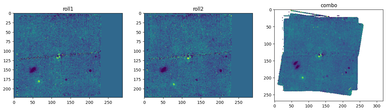
Overlay sky coordinates#
Overlay the RA and Dec grid over the combined rolls
if download_coron_references and docoron3_psflib:
    with fits.open(i2dfiles[0]) as f:
        wcs = WCS(f[1].header)

    # The star coordinates at the time of observation are in the header
    exp_file = uncal_sci_r1_files[0]
    targ_ra = fits.getval(exp_file, 'TARG_RA', 0)
    targ_dec = fits.getval(exp_file, 'TARG_DEC', 0)
    starcoord = SkyCoord(targ_ra, targ_dec, unit='deg', frame='icrs')

    fig, ax = plt.subplots(1, 1, subplot_kw={'projection': wcs})
    vmin, vmax = np.nanquantile(imgs['combo'], [0.01, 0.99])
    ax.imshow(imgs['combo'], vmin=vmin, vmax=vmax)
    ax.scatter(*wcs.world_to_pixel(starcoord),
               marker='x', s=100, c='w')
    ax.grid(True)
WARNING: FITSFixedWarning: 'datfix' made the change 'Set DATE-BEG to '2022-07-17T22:58:10.204' from MJD-BEG.
Set DATE-AVG to '2022-07-18T00:15:08.760' from MJD-AVG.
Set DATE-END to '2022-07-18T01:32:07.316' from MJD-END'. [astropy.wcs.wcs]
WARNING: FITSFixedWarning: 'obsfix' made the change 'Set OBSGEO-L to   -69.981478 from OBSGEO-[XYZ].
Set OBSGEO-B to   -37.692706 from OBSGEO-[XYZ].
Set OBSGEO-H to 1737840324.368 from OBSGEO-[XYZ]'. [astropy.wcs.wcs]
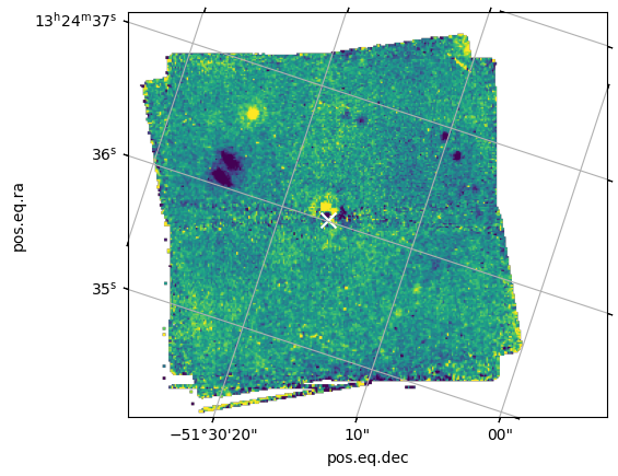
The subtraction is clearly dramatically improved, but we can get a quick quantitative estimate of the comparison between the dedicated reference versus the library by plotting the profiles of the annular standard deviation as a function of separation from the coronagraph center. This is analogous to a contrast curve, but without the normalization for the stellar peak flux. As our science target hasn’t changed, this is a suitable proxy for the improvement in contrast.
def compute_stdev_curves(i2d_file_orig, i2d_file_psflib, mask_circle=None):
    """
    Compute 5-sigma standard deviation curves for two i2d FITS files using CRPIX as center.

    Parameters
    ----------
    i2d_file_orig : str
        Path to the original i2d FITS file.
    i2d_file_psflib : str
        Path to the large-library i2d FITS file.
    mask_circle : tuple, optional
        A tuple of (x, y, radius) in pixels defining a circular region to set
        to NaN before computing the stdev curves. x and y are the center
        of the circle in pixel coordinates (0-indexed).

    Returns
    -------
    radii_arcsec : np.ndarray
        Radii in arcseconds for the stdev curve.
    stdev_orig : np.ndarray
        5-sigma stdev curve for the original library.
    stdev_psflib : np.ndarray
        5-sigma stdev curve for the larger library.
    """

    def load_i2d(filepath):
        with fits.open(filepath) as hdul:
            data = hdul['SCI'].data.astype(float)
            hdr = hdul['SCI'].header
            # CRPIX is 1-indexed, convert to 0-indexed
            cx = hdr.get('CRPIX1', data.shape[1] / 2) - 1
            cy = hdr.get('CRPIX2', data.shape[0] / 2) - 1
            pixelscale = np.sqrt(hdr.get('PIXAR_A2'))
        return data, cx, cy, pixelscale

    def apply_circle_mask(data, mask_circle):
        if mask_circle is not None:
            mx, my, mr = mask_circle
            y, x = np.indices(data.shape)
            dist = np.sqrt((x - mx)**2 + (y - my)**2)
            data = data.copy()
            data[dist <= mr] = np.nan
        return data

    def radial_5sigma_stdev(data, cx, cy):
        y, x = np.indices(data.shape)
        r = np.sqrt((x - cx)**2 + (y - cy)**2).astype(int)

        max_r = int(np.min([cx, cy, data.shape[1] - cx, data.shape[0] - cy]))
        radii = np.arange(1, max_r)
        stdev = np.full(len(radii), np.nan)

        for i, radius in enumerate(radii):
            annulus_mask = r == radius
            annulus_values = data[annulus_mask]
            # Remove NaNs
            annulus_values = annulus_values[np.isfinite(annulus_values)]
            if len(annulus_values) > 2:
                stdev[i] = 5.0 * np.nanstd(annulus_values)

        return radii, stdev

    # Load data
    data_orig, cx_orig, cy_orig, pixelscale_orig = load_i2d(i2d_file_orig)
    data_psflib, cx_psflib, cy_psflib, pixelscale_psflib = load_i2d(i2d_file_psflib)
    if pixelscale_orig != pixelscale_psflib:
        raise ValueError("Pixel scales of the two i2d files do not match.")
    else:
        pixelscale = pixelscale_orig

    # Apply circular mask if provided
    data_orig = apply_circle_mask(data_orig, mask_circle)
    data_psflib = apply_circle_mask(data_psflib, mask_circle)

    # Compute stdev curves
    radii_orig, stdev_orig = radial_5sigma_stdev(data_orig, cx_orig, cy_orig)
    radii_psflib, stdev_psflib = radial_5sigma_stdev(data_psflib, cx_psflib, cy_psflib)

    # Use the shorter of the two radius arrays for comparison
    min_len = min(len(radii_orig), len(radii_psflib))
    radii_arcsec = radii_orig[:min_len] * pixelscale

    return radii_arcsec, stdev_orig[:min_len], stdev_psflib[:min_len]
if download_coron_references and docoron3_psflib:
    # Look for *i2d file in the original coron3 output directory
    i2d_file_orig = sorted(glob.glob(os.path.join(coron3_dir, '*_i2d.fits')))[0]
    i2d_file_psflib = sorted(glob.glob(os.path.join(coron3_psflib_dir, '*_i2d.fits')))[0]

    # Run the stdev calculation, applying a circular mask to reduce the impact of the bright inner planet, HIP 65426 b
    radii_arcsec, stdev_orig, stdev_psflib = compute_stdev_curves(i2d_file_orig, i2d_file_psflib, mask_circle=(131, 138, 6))

    # Make plot of the stdev curves and relative residuals in second panel
    fig, ax = plt.subplots(2, 1, figsize=(8, 6), sharex=True, gridspec_kw={'height_ratios': [3,1]})
    ax[0].plot(radii_arcsec, stdev_orig, label='Dedicated Reference')
    ax[0].plot(radii_arcsec, stdev_psflib, label='PSF Library')
    ax[0].set_yscale('log')
    ax[0].set_ylabel('5$\\sigma$ Annular Standard Deviation')
    ax[0].set_xlim(0, 5)
    ax[0].legend()
    ax[1].plot(radii_arcsec, stdev_orig/stdev_psflib, label='Dedicated / Library')
    ax[1].axhline(1, color='gray', linestyle='--')
    ax[1].set_xlabel('Separation (arcsec)')
    ax[1].set_ylabel('Noise Reduction Factor')
    ax[1].set_xlim(0, 5)
    ax[1].legend()
    plt.tight_layout()
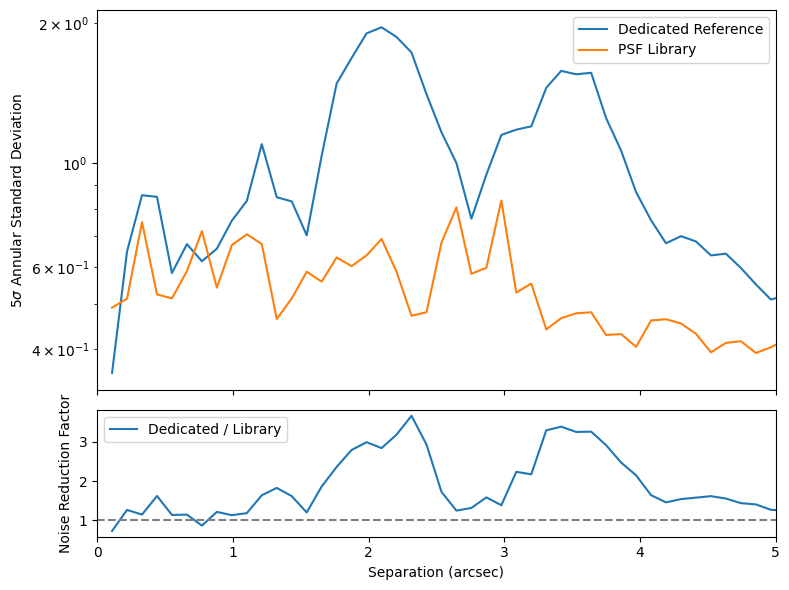
The output images above show that adopting a larger reference library has significantly improved the quality of the PSF subtraction, and the companion exoplanet HIP 65426 b is clearly resolved close to the center of the coronagraph. However, caution should still be taken when adopting such strategies. Even larger PSF libraries may improve the PSF subtraction quality further, but are more computationally demanding, and in some cases the subtraction quality may degrade if the additional PSFs are not suitably matched to the science data. Custom PSF libraries can also be useful when a formal reference target has not been defined for a given science observation.
