
NIRISS SOSS Pipeline Notebook#
Authors: R. Cooper, A. Carter, N. Espinoza, T. Baines
Last Updated: April 17, 2026
Pipeline Version: 2.0.0 (Build 12.3)
Purpose:
This notebook provides a framework for processing Near-Infrared
Imager and Slitless Spectrograph (NIRISS) Single Object Slitless Spectrograph (SOSS) data through all
three James Webb Space Telescope (JWST) pipeline stages. Data is assumed
to be located in one observation folder according to paths set up below.
It should not be necessary to edit any cells other than in the
Configuration section unless modifying the standard
pipeline processing options.
Data:
This notebook uses an example dataset from Early Release Observation (ER0) Program
2734 (PI: K. Pontoppidan).
This program consists of time series observations (TSO) of confirmed exoplanets HAT-P-18b and WASP-96b,
intended to demonstrate the power and precision of the JWST TSO modes. In this notebook, we will reduce the
NIRISS SOSS observations of transiting exoplanet WASP-96b.
Example input data to use will be downloaded automatically unless disabled (i.e., to use local files instead).
JWST pipeline version and CRDS context:
This notebook was written for the above-specified pipeline version and associated
build context for this version of the JWST Calibration Pipeline. Information about
this and other contexts can be found in the JWST Calibration Reference Data System
(CRDS server). If you use different pipeline versions,
please refer to the table here
to determine what context to use. To learn more about the differences for the pipeline,
read the relevant
documentation.
Please note that pipeline software development is a continuous process, so results
in some cases may be slightly different if a subsequent version is used. For optimal
results, users are strongly encouraged to reprocess their data using the most recent
pipeline version and
associated CRDS context,
taking advantage of bug fixes and algorithm improvements.
Any known issues for this build are noted in the notebook.
Visualization:
This notebook uses the batman package (Pypi batman-package) for analysis of the SOSS data.
Some versions of this package may be incompatible with certain python versions and CPU architectures.
If issues are encountered with this package it can be disabled in the ‘Package Imports’ section below;
the function to make the final data product visualization must then be called without the modelparams argument.
Updates:
This notebook is regularly updated as improvements are made to the
pipeline. Find the most up to date version of this notebook at:
https://github.com/spacetelescope/jwst-pipeline-notebooks/
Recent Changes:
November 07, 2025: original notebook released
April 17, 2026: Updated to jwst 2.0.0 (no significant changes)
Table of Contents#
1. Configuration#
Install dependencies and parameters#
To make sure that the pipeline version is compatabile with the steps
discussed below and the required dependencies and packages are installed,
you can create a fresh conda environment and install the provided
requirements.txt file:
conda create -n niriss_soss_pipeline python=3.13
conda activate niriss_soss_pipeline
pip install -r requirements.txt
Set the basic parameters to use with this notebook. These will affect what data is used, where data is located (if already in disk), and pipeline modules run in this data. The list of parameters are:
demo_mode
directories with data
pipeline modules
# Basic import necessary for configuration
import os
demo_mode must be set appropriately below.
Set demo_mode = True to run in demonstration mode. In this
mode this notebook will download example data from the Barbara A.
Mikulski Archive for Space Telescopes (MAST)
and process it through the
pipeline. This will all happen in a local directory unless modified
in Section 3
below.
Set demo_mode = False if you want to process your own data
that has already been downloaded and provide the location of the data.
# Set parameters for demo_mode and processing steps.

# -----------------------------Demo Mode---------------------------------
demo_mode = True

if demo_mode:
    print('Running in demonstration mode using online example data!')

# --------------------------User Mode Directories------------------------
# If demo_mode = False, look for user data in these paths
if not demo_mode:
    # Set directory paths for processing specific data; these will need
    # to be changed to your local directory setup (below are given as
    # examples)
    basedir = os.path.join(os.getcwd(), '')

    # Point to location of science observation data.
    # Assumes uncalibrated data in sci_dir/uncal/ and results in stage1,
    # stage2, stage3 directories
    sci_dir = os.path.join(basedir, 'JWSTData/PID_2734/')

# --------------------------Set Processing Steps--------------------------
# Individual pipeline stages can be turned on/off here.  Note that a later
# stage won't be able to run unless data products have already been
# produced from the prior stage.

# Science processing
dodet1 = True  # calwebb_detector1
dospec2 = True  # calwebb_spec2
dotso3 = True  # calwebb_tso3
doviz = True  # Visualize calwebb_tso3 output
Running in demonstration mode using online example data!
Set CRDS context and server#
Before importing CRDS and JWST modules, we need
to configure our environment. This includes defining a CRDS cache
directory in which to keep the reference files that will be used by the
calibration pipeline.
If the root directory for the local CRDS cache directory has not been set already, it will be set to create one in the home directory.
# ------------------------Set CRDS context and paths----------------------
# Each version of the calibration pipeline is associated with a specific CRDS
# context file. The pipeline will select the appropriate context file behind
# the scenes while running. However, if you wish to override the default context
# file and run the pipeline with a different context, you can set that using
# the CRDS_CONTEXT environment variable. Here we show how this is done,
# although we leave the line commented out in order to use the default context.
# If you wish to specify a different context, uncomment the line below.
#os.environ['CRDS_CONTEXT'] = 'jwst_1464.pmap'  # CRDS context for 1.20.2

# Check whether the local CRDS cache directory has been set.
# If not, set it to the user home directory
if (os.getenv('CRDS_PATH') is None):
    os.environ['CRDS_PATH'] = os.path.join(os.path.expanduser('~'), 'crds')

# Check whether the CRDS server URL has been set.  If not, set it.
if (os.getenv('CRDS_SERVER_URL') is None):
    os.environ['CRDS_SERVER_URL'] = 'https://jwst-crds.stsci.edu'

# Echo CRDS path in use
print(f"CRDS local filepath: {os.environ['CRDS_PATH']}")
print(f"CRDS file server: {os.environ['CRDS_SERVER_URL']}")
CRDS local filepath: /home/runner/crds
CRDS file server: https://jwst-crds.stsci.edu
2. Package Imports#
# Use the entire available screen width for this notebook
from IPython.display import display, HTML
display(HTML("<style>.container { width:95% !important; }</style>"))
# Basic system utilities for interacting with files
# ----------------------General Imports------------------------------------
import glob
import time
import json
from pathlib import Path
from collections import defaultdict

# Numpy for calculations
import numpy as np

# Pandas for loading data into tables
import pandas as pd

# Astroquery for downloading demo files
from astroquery.mast import Observations

# For visualizing data
import matplotlib.pyplot as plt
from astropy.visualization import (ManualInterval, LogStretch,
                                   ImageNormalize, simple_norm)
from astropy.stats import sigma_clip
from astropy.time import Time
import batman # Transit modeling

# For file manipulation
from astropy.io import fits

# For JWST calibration pipeline
import jwst
import crds

from jwst.pipeline import Detector1Pipeline
from jwst.pipeline import Spec2Pipeline
from jwst.pipeline import Tso3Pipeline

# JWST pipeline utilities
from jwst import datamodels
from jwst.associations import asn_from_list  # Tools for creating association files
from jwst.associations.lib.rules_level3_base import DMS_Level3_Base  # Definition of a Lvl3 association file

# Echo pipeline version and CRDS context in use
print(f"JWST Calibration Pipeline Version: {jwst.__version__}")
print(f"Using CRDS Context: {crds.get_context_name('jwst')}")
JWST Calibration Pipeline Version: 2.0.0
CRDS - INFO - Calibration SW Found: jwst 2.0.0 (/home/runner/micromamba/envs/ci-env/lib/python3.13/site-packages/jwst-2.0.0.dist-info)
Using CRDS Context: jwst_1535.pmap
Define convenience functions#
These functions are used within the notebook and assist with selecting certain kinds of input data.
# Sort files into types: TA, spectrum, and F277W
def sort_files(files):
    tafiles = []
    scifiles = []
    f277wfiles = []
    for file in files:
        exptype = fits.getval(file, 'EXP_TYPE')
        filt = fits.getval(file, 'FILTER')
        if ((exptype == 'NIS_TACQ') | (exptype == 'NIS_TACONFIRM')):
            tafiles.append(file)
        if ((exptype == 'NIS_SOSS') & (filt == 'CLEAR')):
            scifiles.append(file)
        if ((exptype == 'NIS_SOSS') & (filt == 'F277W')):
            f277wfiles.append(file)

    return tafiles, scifiles, f277wfiles
# Start a timer to keep track of runtime
time0 = time.perf_counter()
3. Demo Mode Setup (ignore if not using demo data)#
If running in demonstration mode, set up the program information to
retrieve the uncalibrated data automatically from MAST using
astroquery.
MAST has a dedicated service for JWST data retrieval, so the archive can
be searched by instrument keywords rather than just filenames or proposal IDs.
The list of searchable keywords for filtered JWST MAST queries
is here.
For this notebook, we will examine a single TSO of the target, which uses the GR700XD/CLEAR grating/filter combination. Note that the TSO data are typically split into multiple files to faciliate data processing; for more information see the documentation about Segmented Products.
We will start with the uncalibrated data products. The files we are interested in are named
jw02734002001_04101_00001-segNNN_nis_uncal.fits, where NNN refers to the
segment number.
More information about the JWST file naming conventions can be found at: https://jwst-pipeline.readthedocs.io/en/latest/jwst/data_products/file_naming.html
# Set up the program information and paths for demo program
if demo_mode:
    print('Running in demonstration mode and will download example data from MAST!')

    # --------------Program and observation information--------------
    program = '02734'
    instr = 'NIRISS/SOSS'
    filt_pupil = 'CLEAR;GR700XD'
    targname = 'WASP-96'

    # --------------Program and observation directories--------------
    data_dir = os.path.join('.', 'nis_soss_demo_data')
    sci_dir = os.path.join(data_dir, 'PID_2734')
    uncal_dir = os.path.join(sci_dir, 'uncal')  # Uncalibrated pipeline inputs should be here

    if not os.path.exists(uncal_dir):
        os.makedirs(uncal_dir)

    # Create directory if it does not exist
    if not os.path.isdir(data_dir):
        os.mkdir(data_dir)
Running in demonstration mode and will download example data from MAST!
Identify list of science (SCI) uncalibrated files associated with visits.
# Obtain a list of observation IDs for the specified demo program
if demo_mode:
    # Science data
    sci_obs_id_table = Observations.query_criteria(instrument_name=[instr],
                                                   proposal_id=[program],
                                                   filters=[filt_pupil],  # Data for specific filter/pupil
                                                   obs_id=['jw' + program + '*'],
                                                   target_name=targname)
# Turn the list of visits into a list of uncalibrated data files
if demo_mode:
    # Define types of files to select
    file_dict = {'uncal': {'product_type': 'SCIENCE',
                           'productSubGroupDescription': 'UNCAL',
                           'calib_level': [1]}}

    # Science files
    sci_files = []

    # Loop over visits identifying uncalibrated files that are associated
    # with them
    for exposure in (sci_obs_id_table):
        products = Observations.get_product_list(exposure)
        for filetype, query_dict in file_dict.items():
            filtered_products = Observations.filter_products(products, productType=query_dict['product_type'],
                                                             productSubGroupDescription=query_dict['productSubGroupDescription'],
                                                             calib_level=query_dict['calib_level'])
            sci_files.extend(filtered_products['dataURI'])

    print(f"Science files selected for downloading: {len(sci_files)}")
Science files selected for downloading: 8
Download all the uncal files and place them into the appropriate directories.
if demo_mode:
    for filename in sci_files:
        sci_manifest = Observations.download_file(filename,
                                                  local_path=os.path.join(uncal_dir, Path(filename).name))
Downloading URL https://mast.stsci.edu/api/v0.1/Download/file?uri=mast:JWST/product/jw02734002001_04101_00001-seg003_nis_uncal.fits to ./nis_soss_demo_data/PID_2734/uncal/jw02734002001_04101_00001-seg003_nis_uncal.fits ...
[Done]
Downloading URL https://mast.stsci.edu/api/v0.1/Download/file?uri=mast:JWST/product/jw02734002001_02101_00004-seg001_nis_uncal.fits to ./nis_soss_demo_data/PID_2734/uncal/jw02734002001_02101_00004-seg001_nis_uncal.fits ...
[Done]
Downloading URL https://mast.stsci.edu/api/v0.1/Download/file?uri=mast:JWST/product/jw02734002001_04101_00001-seg002_nis_uncal.fits to ./nis_soss_demo_data/PID_2734/uncal/jw02734002001_04101_00001-seg002_nis_uncal.fits ...
[Done]
Downloading URL https://mast.stsci.edu/api/v0.1/Download/file?uri=mast:JWST/product/jw02734002001_02101_00002-seg001_nis_uncal.fits to ./nis_soss_demo_data/PID_2734/uncal/jw02734002001_02101_00002-seg001_nis_uncal.fits ...
[Done]
Downloading URL https://mast.stsci.edu/api/v0.1/Download/file?uri=mast:JWST/product/jw02734002001_02101_00001-seg001_nis_uncal.fits to ./nis_soss_demo_data/PID_2734/uncal/jw02734002001_02101_00001-seg001_nis_uncal.fits ...
[Done]
Downloading URL https://mast.stsci.edu/api/v0.1/Download/file?uri=mast:JWST/product/jw02734002001_04101_00001-seg001_nis_uncal.fits to ./nis_soss_demo_data/PID_2734/uncal/jw02734002001_04101_00001-seg001_nis_uncal.fits ...
[Done]
Downloading URL https://mast.stsci.edu/api/v0.1/Download/file?uri=mast:JWST/product/jw02734002001_02101_00003-seg001_nis_uncal.fits to ./nis_soss_demo_data/PID_2734/uncal/jw02734002001_02101_00003-seg001_nis_uncal.fits ...
[Done]
Downloading URL https://mast.stsci.edu/api/v0.1/Download/file?uri=mast:JWST/product/jw02734002001_04102_00001-seg001_nis_uncal.fits to ./nis_soss_demo_data/PID_2734/uncal/jw02734002001_04102_00001-seg001_nis_uncal.fits ...
[Done]
4. Directory Setup#
Set up detailed paths to input/output stages here.
# Define output subdirectories to keep science data products organized
# -----------------------------Science Directories------------------------------
uncal_dir = os.path.join(sci_dir, 'uncal')  # Uncalibrated pipeline inputs should be here
det1_dir = os.path.join(sci_dir, 'stage1')  # calwebb_detector1 pipeline outputs will go here
spec2_dir = os.path.join(sci_dir, 'stage2')  # calwebb_spec2 pipeline outputs will go here
tso3_dir = os.path.join(sci_dir, 'stage3')  # calwebb_tso3 pipeline outputs will go here

# We need to check that the desired output directories exist, and if not create them
# Ensure filepaths for input data exist
if not os.path.exists(uncal_dir):
    os.makedirs(uncal_dir)

if not os.path.exists(det1_dir):
    os.makedirs(det1_dir)
if not os.path.exists(spec2_dir):
    os.makedirs(spec2_dir)
if not os.path.exists(tso3_dir):
    os.makedirs(tso3_dir)
Print the exposure parameters of all potential input files:
uncal_files = sorted(glob.glob(os.path.join(uncal_dir, '*_uncal.fits')))

for file in uncal_files:
    model = datamodels.open(file)
    # print file name
    print(model.meta.filename)
    # Print out exposure info
    print(f"Instrument: {model.meta.instrument.name}")
    print(f"Filter: {model.meta.instrument.filter}")
    print(f"Pupil: {model.meta.instrument.pupil}")
    print(f"Exposure type: {model.meta.exposure.type}")
    print(f"Total number of integrations: {model.meta.exposure.nints}")
    if model.meta.exposure.nints != 1:
        print(f"Integration range: {model.meta.exposure.integration_start}-{model.meta.exposure.integration_end}")
    print(f"Exposure start time (UTC): {Time(model.meta.exposure.start_time, format='mjd').fits}")
    print(f"Number of groups: {model.meta.exposure.ngroups}")
    print(f"Readout pattern: {model.meta.exposure.readpatt}")
    print("\n")
    model.close()
jw02734002001_02101_00001-seg001_nis_uncal.fits
Instrument: NIRISS
Filter: F480M
Pupil: CLEARP
Exposure type: NIS_TACQ
Total number of integrations: 1
Exposure start time (UTC): 2022-06-21T03:48:43.106
Number of groups: 19
Readout pattern: NISRAPID


jw02734002001_02101_00002-seg001_nis_uncal.fits
Instrument: NIRISS
Filter: F480M
Pupil: CLEARP
Exposure type: NIS_TACQ
Total number of integrations: 1
Exposure start time (UTC): 2022-06-21T03:49:57.794
Number of groups: 19
Readout pattern: NISRAPID


jw02734002001_02101_00003-seg001_nis_uncal.fits
Instrument: NIRISS
Filter: F480M
Pupil: CLEARP
Exposure type: NIS_TACQ
Total number of integrations: 1
Exposure start time (UTC): 2022-06-21T03:51:11.586
Number of groups: 19
Readout pattern: NISRAPID


jw02734002001_02101_00004-seg001_nis_uncal.fits
Instrument: NIRISS
Filter: F480M
Pupil: CLEARP
Exposure type: NIS_TACONFIRM
Total number of integrations: 1
Exposure start time (UTC): 2022-06-21T03:58:01.825
Number of groups: 19
Readout pattern: NISRAPID
jw02734002001_04101_00001-seg001_nis_uncal.fits
Instrument: NIRISS
Filter: CLEAR
Pupil: GR700XD
Exposure type: NIS_SOSS
Total number of integrations: 280
Integration range: 1-96
Exposure start time (UTC): 2022-06-21T04:06:18.164
Number of groups: 14
Readout pattern: NISRAPID
jw02734002001_04101_00001-seg002_nis_uncal.fits
Instrument: NIRISS
Filter: CLEAR
Pupil: GR700XD
Exposure type: NIS_SOSS
Total number of integrations: 280
Integration range: 97-188
Exposure start time (UTC): 2022-06-21T04:06:18.164
Number of groups: 14
Readout pattern: NISRAPID
jw02734002001_04101_00001-seg003_nis_uncal.fits
Instrument: NIRISS
Filter: CLEAR
Pupil: GR700XD
Exposure type: NIS_SOSS
Total number of integrations: 280
Integration range: 189-280
Exposure start time (UTC): 2022-06-21T04:06:18.164
Number of groups: 14
Readout pattern: NISRAPID


jw02734002001_04102_00001-seg001_nis_uncal.fits
Instrument: NIRISS
Filter: F277W
Pupil: GR700XD
Exposure type: NIS_SOSS
Total number of integrations: 11
Integration range: 1-11
Exposure start time (UTC): 2022-06-21T10:32:46.938
Number of groups: 14
Readout pattern: NISRAPID
Since this is a NIRISS SOSS observation, the first four files are target aquisition (TA) exposures.
Target acquisition is performed in a 64x64 pixel subarray before the target is moved
to its position in the science subarray. The TA exposures have exposure type NIS_TACQ or NIS_TACONFIRM and use the F480M filter.
These exposures, particularly the final confirmation image, can be helpful for diagnosing potential problems with the data.
For more information about the SOSS TA procedure, see the NIRISS TA documentation.
The following three exposures are our time series observation, split into three segments: seg001 through seg003 in the filenames. These exposures use the CLEAR/GR700XD filter/pupil combination and consist of 280 integrations in total, each composed of 14 groups up the ramp, corresponding to a total exposure time of 6.41 hours.
Each exposure uses the NISRAPID readout pattern.
The final exposure uses the F277W filter and was obtained because it is useful for masking order-zero sources and to isolate the first spectral order in the $2.4 \ \mu m-2.8 \ \mu m$ wavelength range, where they overlap significantly in the CLEAR exposures. We will process the F277W exposure through stage 1 in this notebook, but the background subtraction step in the second stage does not currently work with these exposures.
For more information about how JWST exposures are defined by up-the-ramp sampling, see the Understanding Exposure Times JDox article.
In this notebook, we will focus on processing the CLEAR/GR700XD exposures (though we will also process the single F277W exposure through Stage 1), so we can update the list of uncalibrated files to remove the TA exposures:
# Print out the time benchmark
time1 = time.perf_counter()
print(f"Runtime so far: {time1 - time0:0.0f} seconds")
Runtime so far: 92 seconds
5. Detector1 Pipeline#
Run the data through the
Detector1
stage of the pipeline to apply detector level calibrations and create a
countrate data product where slopes are fitted to the integration ramps.
These _rateints.fits products are 3D (nintegrations x nrows x ncols)
and contain the fitted ramp slopes for each integration.
2D countrate data products (_rate.fits) are also
created (nrows x ncols) which have been averaged over all
integrations.
The following Detector1 steps are available for NIRISS SOSS:
group_scaledq_initsaturationsuperbiasrefpixlinearitydark_currentjumpclean_flicker_noiseramp_fitgain_scale
By default, these Detector1 steps are currently skipped for NIRISS SOSS exposures: group_scale, clean_flicker_noise, and gain_scale.
Each observing mode of JWST has different requirements when it comes to correcting for detector effects.
The clean_flicker_noise step was designed to remove 1/f noise from calibrated ramp images, but SOSS
users have found its performance insufficient due to the lack of non-illuminated
background pixels in the SOSS subarrays. A more rigorous group-level subtraction is likely needed, and is currently in development by the SOSS team.
By default, this step is currently skipped.
It is also unclear whether TSO science benefits from the dark current step in its current implementation. In the following example we leave the step on, but it can easily be turned off as shown.
For more information about each step and a full list of step arguments, please refer to the official documentation on ReadtheDocs.
# Set up a dictionary to define how the Detector1 pipeline should be configured

# Boilerplate dictionary setup
det1dict = defaultdict(dict)

# Step names are copied here for reference
det1_steps = ['group_scale', 'dq_init', 'saturation', 'superbias', 'refpix',
              'linearity', 'dark_current', 'jump', 'clean_flicker_noise',
              'ramp_fit', 'gain_scale']

# Overrides for whether or not certain steps should be skipped
# Optionally, skip the dark step
# det1dict['dark_current']['skip'] = True

# Overrides for various reference files
# Files should be in the base local directory or provide full path
#det1dict['dq_init']['override_mask'] = 'myfile.fits'  # Bad pixel mask
#det1dict['saturation']['override_saturation'] = 'myfile.fits'  # Saturation
#det1dict['linearity']['override_linearity'] = 'myfile.fits'  # Linearity
#det1dict['dark_current']['override_dark'] = 'myfile.fits'  # Dark current subtraction
#det1dict['jump']['override_gain'] = 'myfile.fits'  # Gain used by jump step
#det1dict['ramp_fit']['override_gain'] = 'myfile.fits'  # Gain used by ramp fitting step
#det1dict['jump']['override_readnoise'] = 'myfile.fits'  # Read noise used by jump step
#det1dict['ramp_fit']['override_readnoise'] = 'myfile.fits'  # Read noise used by ramp fitting step

# Turn on multi-core processing (off by default). Choose what fraction of cores to use (quarter, half, or all)
det1dict['jump']['maximum_cores'] = 'half'
Run Detector1 stage of pipeline:
# Run Detector1 stage of pipeline, specifying:
# output directory to save *_rateints.fits files
# save_results flag set to True so the *rateints.fits files are saved

if dodet1:
    for uncal in uncal_files:
        rate_result = Detector1Pipeline.call(uncal,
                                             output_dir=det1_dir,
                                             steps=det1dict,
                                             save_results=True)
else:
    print('Skipping Detector1 processing')
2026-04-15 20:16:32,802 - CRDS - INFO - Fetching /home/runner/crds/mappings/jwst/jwst_system_datalvl_0002.rmap 694 bytes (1 / 224 files) (0 / 796.2 K bytes)
2026-04-15 20:16:33,035 - CRDS - INFO - Fetching /home/runner/crds/mappings/jwst/jwst_system_calver_0069.rmap 5.8 K bytes (2 / 224 files) (694 / 796.2 K bytes)
2026-04-15 20:16:33,251 - CRDS - INFO - Fetching /home/runner/crds/mappings/jwst/jwst_system_0064.imap 385 bytes (3 / 224 files) (6.5 K / 796.2 K bytes)
2026-04-15 20:16:33,471 - CRDS - INFO - Fetching /home/runner/crds/mappings/jwst/jwst_nirspec_wavelengthrange_0024.rmap 1.4 K bytes (4 / 224 files) (6.9 K / 796.2 K bytes)
2026-04-15 20:16:33,684 - CRDS - INFO - Fetching /home/runner/crds/mappings/jwst/jwst_nirspec_wavecorr_0005.rmap 884 bytes (5 / 224 files) (8.3 K / 796.2 K bytes)
2026-04-15 20:16:33,919 - CRDS - INFO - Fetching /home/runner/crds/mappings/jwst/jwst_nirspec_superbias_0089.rmap 39.4 K bytes (6 / 224 files) (9.1 K / 796.2 K bytes)
2026-04-15 20:16:34,203 - CRDS - INFO - Fetching /home/runner/crds/mappings/jwst/jwst_nirspec_sirskernel_0002.rmap 704 bytes (7 / 224 files) (48.5 K / 796.2 K bytes)
2026-04-15 20:16:34,445 - CRDS - INFO - Fetching /home/runner/crds/mappings/jwst/jwst_nirspec_sflat_0027.rmap 20.6 K bytes (8 / 224 files) (49.2 K / 796.2 K bytes)
2026-04-15 20:16:34,734 - CRDS - INFO - Fetching /home/runner/crds/mappings/jwst/jwst_nirspec_saturation_0018.rmap 2.0 K bytes (9 / 224 files) (69.8 K / 796.2 K bytes)
2026-04-15 20:16:34,949 - CRDS - INFO - Fetching /home/runner/crds/mappings/jwst/jwst_nirspec_refpix_0015.rmap 1.6 K bytes (10 / 224 files) (71.9 K / 796.2 K bytes)
2026-04-15 20:16:35,195 - CRDS - INFO - Fetching /home/runner/crds/mappings/jwst/jwst_nirspec_readnoise_0025.rmap 2.6 K bytes (11 / 224 files) (73.4 K / 796.2 K bytes)
2026-04-15 20:16:35,427 - CRDS - INFO - Fetching /home/runner/crds/mappings/jwst/jwst_nirspec_psf_0002.rmap 687 bytes (12 / 224 files) (76.0 K / 796.2 K bytes)
2026-04-15 20:16:35,653 - CRDS - INFO - Fetching /home/runner/crds/mappings/jwst/jwst_nirspec_pictureframe_0002.rmap 886 bytes (13 / 224 files) (76.7 K / 796.2 K bytes)
2026-04-15 20:16:35,876 - CRDS - INFO - Fetching /home/runner/crds/mappings/jwst/jwst_nirspec_photom_0013.rmap 958 bytes (14 / 224 files) (77.6 K / 796.2 K bytes)
2026-04-15 20:16:36,098 - CRDS - INFO - Fetching /home/runner/crds/mappings/jwst/jwst_nirspec_pathloss_0011.rmap 1.2 K bytes (15 / 224 files) (78.5 K / 796.2 K bytes)
2026-04-15 20:16:36,314 - CRDS - INFO - Fetching /home/runner/crds/mappings/jwst/jwst_nirspec_pars-whitelightstep_0001.rmap 777 bytes (16 / 224 files) (79.7 K / 796.2 K bytes)
2026-04-15 20:16:36,542 - CRDS - INFO - Fetching /home/runner/crds/mappings/jwst/jwst_nirspec_pars-tso3pipeline_0001.rmap 786 bytes (17 / 224 files) (80.5 K / 796.2 K bytes)
2026-04-15 20:16:36,766 - CRDS - INFO - Fetching /home/runner/crds/mappings/jwst/jwst_nirspec_pars-spec2pipeline_0013.rmap 2.1 K bytes (18 / 224 files) (81.3 K / 796.2 K bytes)
2026-04-15 20:16:36,987 - CRDS - INFO - Fetching /home/runner/crds/mappings/jwst/jwst_nirspec_pars-resamplespecstep_0002.rmap 709 bytes (19 / 224 files) (83.4 K / 796.2 K bytes)
2026-04-15 20:16:37,203 - CRDS - INFO - Fetching /home/runner/crds/mappings/jwst/jwst_nirspec_pars-refpixstep_0003.rmap 910 bytes (20 / 224 files) (84.1 K / 796.2 K bytes)
2026-04-15 20:16:37,421 - CRDS - INFO - Fetching /home/runner/crds/mappings/jwst/jwst_nirspec_pars-pixelreplacestep_0001.rmap 818 bytes (21 / 224 files) (85.0 K / 796.2 K bytes)
2026-04-15 20:16:37,658 - CRDS - INFO - Fetching /home/runner/crds/mappings/jwst/jwst_nirspec_pars-pictureframestep_0001.rmap 818 bytes (22 / 224 files) (85.8 K / 796.2 K bytes)
2026-04-15 20:16:37,876 - CRDS - INFO - Fetching /home/runner/crds/mappings/jwst/jwst_nirspec_pars-outlierdetectionstep_0005.rmap 1.1 K bytes (23 / 224 files) (86.7 K / 796.2 K bytes)
2026-04-15 20:16:38,093 - CRDS - INFO - Fetching /home/runner/crds/mappings/jwst/jwst_nirspec_pars-jumpstep_0006.rmap 810 bytes (24 / 224 files) (87.8 K / 796.2 K bytes)
2026-04-15 20:16:38,316 - CRDS - INFO - Fetching /home/runner/crds/mappings/jwst/jwst_nirspec_pars-image2pipeline_0008.rmap 1.0 K bytes (25 / 224 files) (88.6 K / 796.2 K bytes)
2026-04-15 20:16:38,536 - CRDS - INFO - Fetching /home/runner/crds/mappings/jwst/jwst_nirspec_pars-extract1dstep_0001.rmap 794 bytes (26 / 224 files) (89.6 K / 796.2 K bytes)
2026-04-15 20:16:38,762 - CRDS - INFO - Fetching /home/runner/crds/mappings/jwst/jwst_nirspec_pars-detector1pipeline_0004.rmap 1.1 K bytes (27 / 224 files) (90.4 K / 796.2 K bytes)
2026-04-15 20:16:38,974 - CRDS - INFO - Fetching /home/runner/crds/mappings/jwst/jwst_nirspec_pars-darkpipeline_0003.rmap 872 bytes (28 / 224 files) (91.5 K / 796.2 K bytes)
2026-04-15 20:16:39,205 - CRDS - INFO - Fetching /home/runner/crds/mappings/jwst/jwst_nirspec_pars-darkcurrentstep_0003.rmap 1.8 K bytes (29 / 224 files) (92.4 K / 796.2 K bytes)
2026-04-15 20:16:39,433 - CRDS - INFO - Fetching /home/runner/crds/mappings/jwst/jwst_nirspec_pars-cubebuildstep_0001.rmap 862 bytes (30 / 224 files) (94.2 K / 796.2 K bytes)
2026-04-15 20:16:39,656 - CRDS - INFO - Fetching /home/runner/crds/mappings/jwst/jwst_nirspec_pars-cleanflickernoisestep_0002.rmap 983 bytes (31 / 224 files) (95.1 K / 796.2 K bytes)
2026-04-15 20:16:39,873 - CRDS - INFO - Fetching /home/runner/crds/mappings/jwst/jwst_nirspec_pars-adaptivetracemodelstep_0002.rmap 997 bytes (32 / 224 files) (96.1 K / 796.2 K bytes)
2026-04-15 20:16:40,082 - CRDS - INFO - Fetching /home/runner/crds/mappings/jwst/jwst_nirspec_ote_0030.rmap 1.3 K bytes (33 / 224 files) (97.1 K / 796.2 K bytes)
2026-04-15 20:16:40,294 - CRDS - INFO - Fetching /home/runner/crds/mappings/jwst/jwst_nirspec_msaoper_0018.rmap 1.6 K bytes (34 / 224 files) (98.3 K / 796.2 K bytes)
2026-04-15 20:16:40,524 - CRDS - INFO - Fetching /home/runner/crds/mappings/jwst/jwst_nirspec_msa_0027.rmap 1.3 K bytes (35 / 224 files) (100.0 K / 796.2 K bytes)
2026-04-15 20:16:40,766 - CRDS - INFO - Fetching /home/runner/crds/mappings/jwst/jwst_nirspec_mask_0045.rmap 4.9 K bytes (36 / 224 files) (101.2 K / 796.2 K bytes)
2026-04-15 20:16:40,978 - CRDS - INFO - Fetching /home/runner/crds/mappings/jwst/jwst_nirspec_linearity_0017.rmap 1.6 K bytes (37 / 224 files) (106.2 K / 796.2 K bytes)
2026-04-15 20:16:41,194 - CRDS - INFO - Fetching /home/runner/crds/mappings/jwst/jwst_nirspec_ipc_0006.rmap 876 bytes (38 / 224 files) (107.7 K / 796.2 K bytes)
2026-04-15 20:16:41,414 - CRDS - INFO - Fetching /home/runner/crds/mappings/jwst/jwst_nirspec_ifuslicer_0018.rmap 1.5 K bytes (39 / 224 files) (108.6 K / 796.2 K bytes)
2026-04-15 20:16:41,643 - CRDS - INFO - Fetching /home/runner/crds/mappings/jwst/jwst_nirspec_ifupost_0020.rmap 1.5 K bytes (40 / 224 files) (110.1 K / 796.2 K bytes)
2026-04-15 20:16:41,855 - CRDS - INFO - Fetching /home/runner/crds/mappings/jwst/jwst_nirspec_ifufore_0017.rmap 1.5 K bytes (41 / 224 files) (111.6 K / 796.2 K bytes)
2026-04-15 20:16:42,071 - CRDS - INFO - Fetching /home/runner/crds/mappings/jwst/jwst_nirspec_gain_0023.rmap 1.8 K bytes (42 / 224 files) (113.1 K / 796.2 K bytes)
2026-04-15 20:16:42,299 - CRDS - INFO - Fetching /home/runner/crds/mappings/jwst/jwst_nirspec_fpa_0028.rmap 1.3 K bytes (43 / 224 files) (114.9 K / 796.2 K bytes)
2026-04-15 20:16:42,519 - CRDS - INFO - Fetching /home/runner/crds/mappings/jwst/jwst_nirspec_fore_0026.rmap 5.0 K bytes (44 / 224 files) (116.2 K / 796.2 K bytes)
2026-04-15 20:16:42,736 - CRDS - INFO - Fetching /home/runner/crds/mappings/jwst/jwst_nirspec_flat_0015.rmap 3.8 K bytes (45 / 224 files) (121.1 K / 796.2 K bytes)
2026-04-15 20:16:42,964 - CRDS - INFO - Fetching /home/runner/crds/mappings/jwst/jwst_nirspec_fflat_0030.rmap 7.2 K bytes (46 / 224 files) (124.9 K / 796.2 K bytes)
2026-04-15 20:16:43,184 - CRDS - INFO - Fetching /home/runner/crds/mappings/jwst/jwst_nirspec_extract1d_0018.rmap 2.3 K bytes (47 / 224 files) (132.1 K / 796.2 K bytes)
2026-04-15 20:16:43,412 - CRDS - INFO - Fetching /home/runner/crds/mappings/jwst/jwst_nirspec_disperser_0028.rmap 5.7 K bytes (48 / 224 files) (134.4 K / 796.2 K bytes)
2026-04-15 20:16:43,643 - CRDS - INFO - Fetching /home/runner/crds/mappings/jwst/jwst_nirspec_dflat_0007.rmap 1.1 K bytes (49 / 224 files) (140.1 K / 796.2 K bytes)
2026-04-15 20:16:43,855 - CRDS - INFO - Fetching /home/runner/crds/mappings/jwst/jwst_nirspec_dark_0085.rmap 37.4 K bytes (50 / 224 files) (141.3 K / 796.2 K bytes)
2026-04-15 20:16:44,137 - CRDS - INFO - Fetching /home/runner/crds/mappings/jwst/jwst_nirspec_cubepar_0015.rmap 966 bytes (51 / 224 files) (178.7 K / 796.2 K bytes)
2026-04-15 20:16:44,351 - CRDS - INFO - Fetching /home/runner/crds/mappings/jwst/jwst_nirspec_collimator_0026.rmap 1.3 K bytes (52 / 224 files) (179.6 K / 796.2 K bytes)
2026-04-15 20:16:44,587 - CRDS - INFO - Fetching /home/runner/crds/mappings/jwst/jwst_nirspec_camera_0026.rmap 1.3 K bytes (53 / 224 files) (181.0 K / 796.2 K bytes)
2026-04-15 20:16:44,795 - CRDS - INFO - Fetching /home/runner/crds/mappings/jwst/jwst_nirspec_barshadow_0007.rmap 1.8 K bytes (54 / 224 files) (182.3 K / 796.2 K bytes)
2026-04-15 20:16:45,010 - CRDS - INFO - Fetching /home/runner/crds/mappings/jwst/jwst_nirspec_area_0019.rmap 6.8 K bytes (55 / 224 files) (184.1 K / 796.2 K bytes)
2026-04-15 20:16:45,228 - CRDS - INFO - Fetching /home/runner/crds/mappings/jwst/jwst_nirspec_apcorr_0009.rmap 5.6 K bytes (56 / 224 files) (190.9 K / 796.2 K bytes)
2026-04-15 20:16:45,458 - CRDS - INFO - Fetching /home/runner/crds/mappings/jwst/jwst_nirspec_0432.imap 6.2 K bytes (57 / 224 files) (196.5 K / 796.2 K bytes)
2026-04-15 20:16:45,666 - CRDS - INFO - Fetching /home/runner/crds/mappings/jwst/jwst_niriss_wavelengthrange_0008.rmap 897 bytes (58 / 224 files) (202.6 K / 796.2 K bytes)
2026-04-15 20:16:45,884 - CRDS - INFO - Fetching /home/runner/crds/mappings/jwst/jwst_niriss_trappars_0004.rmap 753 bytes (59 / 224 files) (203.5 K / 796.2 K bytes)
2026-04-15 20:16:46,110 - CRDS - INFO - Fetching /home/runner/crds/mappings/jwst/jwst_niriss_trapdensity_0005.rmap 705 bytes (60 / 224 files) (204.3 K / 796.2 K bytes)
2026-04-15 20:16:46,318 - CRDS - INFO - Fetching /home/runner/crds/mappings/jwst/jwst_niriss_throughput_0005.rmap 1.3 K bytes (61 / 224 files) (205.0 K / 796.2 K bytes)
2026-04-15 20:16:46,536 - CRDS - INFO - Fetching /home/runner/crds/mappings/jwst/jwst_niriss_superbias_0035.rmap 8.3 K bytes (62 / 224 files) (206.2 K / 796.2 K bytes)
2026-04-15 20:16:46,766 - CRDS - INFO - Fetching /home/runner/crds/mappings/jwst/jwst_niriss_specwcs_0017.rmap 3.1 K bytes (63 / 224 files) (214.5 K / 796.2 K bytes)
2026-04-15 20:16:46,979 - CRDS - INFO - Fetching /home/runner/crds/mappings/jwst/jwst_niriss_specprofile_0010.rmap 2.5 K bytes (64 / 224 files) (217.7 K / 796.2 K bytes)
2026-04-15 20:16:47,189 - CRDS - INFO - Fetching /home/runner/crds/mappings/jwst/jwst_niriss_speckernel_0006.rmap 1.0 K bytes (65 / 224 files) (220.2 K / 796.2 K bytes)
2026-04-15 20:16:47,405 - CRDS - INFO - Fetching /home/runner/crds/mappings/jwst/jwst_niriss_sirskernel_0002.rmap 700 bytes (66 / 224 files) (221.2 K / 796.2 K bytes)
2026-04-15 20:16:47,634 - CRDS - INFO - Fetching /home/runner/crds/mappings/jwst/jwst_niriss_saturation_0015.rmap 829 bytes (67 / 224 files) (221.9 K / 796.2 K bytes)
2026-04-15 20:16:47,842 - CRDS - INFO - Fetching /home/runner/crds/mappings/jwst/jwst_niriss_readnoise_0011.rmap 987 bytes (68 / 224 files) (222.7 K / 796.2 K bytes)
2026-04-15 20:16:48,069 - CRDS - INFO - Fetching /home/runner/crds/mappings/jwst/jwst_niriss_photom_0041.rmap 1.3 K bytes (69 / 224 files) (223.7 K / 796.2 K bytes)
2026-04-15 20:16:48,278 - CRDS - INFO - Fetching /home/runner/crds/mappings/jwst/jwst_niriss_persat_0007.rmap 674 bytes (70 / 224 files) (225.0 K / 796.2 K bytes)
2026-04-15 20:16:48,498 - CRDS - INFO - Fetching /home/runner/crds/mappings/jwst/jwst_niriss_pathloss_0003.rmap 758 bytes (71 / 224 files) (225.6 K / 796.2 K bytes)
2026-04-15 20:16:48,713 - CRDS - INFO - Fetching /home/runner/crds/mappings/jwst/jwst_niriss_pastasoss_0006.rmap 818 bytes (72 / 224 files) (226.4 K / 796.2 K bytes)
2026-04-15 20:16:48,941 - CRDS - INFO - Fetching /home/runner/crds/mappings/jwst/jwst_niriss_pars-wfsscontamstep_0001.rmap 797 bytes (73 / 224 files) (227.2 K / 796.2 K bytes)
2026-04-15 20:16:49,169 - CRDS - INFO - Fetching /home/runner/crds/mappings/jwst/jwst_niriss_pars-undersamplecorrectionstep_0001.rmap 904 bytes (74 / 224 files) (228.0 K / 796.2 K bytes)
2026-04-15 20:16:49,406 - CRDS - INFO - Fetching /home/runner/crds/mappings/jwst/jwst_niriss_pars-tweakregstep_0012.rmap 3.1 K bytes (75 / 224 files) (228.9 K / 796.2 K bytes)
2026-04-15 20:16:49,627 - CRDS - INFO - Fetching /home/runner/crds/mappings/jwst/jwst_niriss_pars-spec2pipeline_0009.rmap 1.2 K bytes (76 / 224 files) (232.0 K / 796.2 K bytes)
2026-04-15 20:16:49,844 - CRDS - INFO - Fetching /home/runner/crds/mappings/jwst/jwst_niriss_pars-sourcecatalogstep_0002.rmap 2.3 K bytes (77 / 224 files) (233.3 K / 796.2 K bytes)
2026-04-15 20:16:50,060 - CRDS - INFO - Fetching /home/runner/crds/mappings/jwst/jwst_niriss_pars-resamplestep_0002.rmap 687 bytes (78 / 224 files) (235.6 K / 796.2 K bytes)
2026-04-15 20:16:50,296 - CRDS - INFO - Fetching /home/runner/crds/mappings/jwst/jwst_niriss_pars-outlierdetectionstep_0004.rmap 2.7 K bytes (79 / 224 files) (236.3 K / 796.2 K bytes)
2026-04-15 20:16:50,525 - CRDS - INFO - Fetching /home/runner/crds/mappings/jwst/jwst_niriss_pars-jumpstep_0007.rmap 6.4 K bytes (80 / 224 files) (239.0 K / 796.2 K bytes)
2026-04-15 20:16:50,740 - CRDS - INFO - Fetching /home/runner/crds/mappings/jwst/jwst_niriss_pars-image2pipeline_0005.rmap 1.0 K bytes (81 / 224 files) (245.3 K / 796.2 K bytes)
2026-04-15 20:16:50,959 - CRDS - INFO - Fetching /home/runner/crds/mappings/jwst/jwst_niriss_pars-detector1pipeline_0005.rmap 1.5 K bytes (82 / 224 files) (246.3 K / 796.2 K bytes)
2026-04-15 20:16:51,198 - CRDS - INFO - Fetching /home/runner/crds/mappings/jwst/jwst_niriss_pars-darkpipeline_0002.rmap 868 bytes (83 / 224 files) (247.9 K / 796.2 K bytes)
2026-04-15 20:16:51,409 - CRDS - INFO - Fetching /home/runner/crds/mappings/jwst/jwst_niriss_pars-darkcurrentstep_0001.rmap 591 bytes (84 / 224 files) (248.8 K / 796.2 K bytes)
2026-04-15 20:16:51,639 - CRDS - INFO - Fetching /home/runner/crds/mappings/jwst/jwst_niriss_pars-cleanflickernoisestep_0003.rmap 1.2 K bytes (85 / 224 files) (249.3 K / 796.2 K bytes)
2026-04-15 20:16:51,869 - CRDS - INFO - Fetching /home/runner/crds/mappings/jwst/jwst_niriss_pars-chargemigrationstep_0005.rmap 5.7 K bytes (86 / 224 files) (250.6 K / 796.2 K bytes)
2026-04-15 20:16:52,076 - CRDS - INFO - Fetching /home/runner/crds/mappings/jwst/jwst_niriss_pars-backgroundstep_0003.rmap 822 bytes (87 / 224 files) (256.2 K / 796.2 K bytes)
2026-04-15 20:16:52,294 - CRDS - INFO - Fetching /home/runner/crds/mappings/jwst/jwst_niriss_nrm_0005.rmap 663 bytes (88 / 224 files) (257.0 K / 796.2 K bytes)
2026-04-15 20:16:52,509 - CRDS - INFO - Fetching /home/runner/crds/mappings/jwst/jwst_niriss_mask_0025.rmap 1.6 K bytes (89 / 224 files) (257.7 K / 796.2 K bytes)
2026-04-15 20:16:52,720 - CRDS - INFO - Fetching /home/runner/crds/mappings/jwst/jwst_niriss_linearity_0022.rmap 961 bytes (90 / 224 files) (259.3 K / 796.2 K bytes)
2026-04-15 20:16:52,937 - CRDS - INFO - Fetching /home/runner/crds/mappings/jwst/jwst_niriss_ipc_0007.rmap 651 bytes (91 / 224 files) (260.3 K / 796.2 K bytes)
2026-04-15 20:16:53,162 - CRDS - INFO - Fetching /home/runner/crds/mappings/jwst/jwst_niriss_gain_0011.rmap 797 bytes (92 / 224 files) (260.9 K / 796.2 K bytes)
2026-04-15 20:16:53,368 - CRDS - INFO - Fetching /home/runner/crds/mappings/jwst/jwst_niriss_flat_0023.rmap 5.9 K bytes (93 / 224 files) (261.7 K / 796.2 K bytes)
2026-04-15 20:16:53,586 - CRDS - INFO - Fetching /home/runner/crds/mappings/jwst/jwst_niriss_filteroffset_0010.rmap 853 bytes (94 / 224 files) (267.6 K / 796.2 K bytes)
2026-04-15 20:16:53,794 - CRDS - INFO - Fetching /home/runner/crds/mappings/jwst/jwst_niriss_extract1d_0007.rmap 905 bytes (95 / 224 files) (268.4 K / 796.2 K bytes)
2026-04-15 20:16:54,012 - CRDS - INFO - Fetching /home/runner/crds/mappings/jwst/jwst_niriss_drizpars_0004.rmap 519 bytes (96 / 224 files) (269.3 K / 796.2 K bytes)
2026-04-15 20:16:54,222 - CRDS - INFO - Fetching /home/runner/crds/mappings/jwst/jwst_niriss_distortion_0025.rmap 3.4 K bytes (97 / 224 files) (269.9 K / 796.2 K bytes)
2026-04-15 20:16:54,432 - CRDS - INFO - Fetching /home/runner/crds/mappings/jwst/jwst_niriss_dark_0039.rmap 8.3 K bytes (98 / 224 files) (273.3 K / 796.2 K bytes)
2026-04-15 20:16:54,649 - CRDS - INFO - Fetching /home/runner/crds/mappings/jwst/jwst_niriss_bkg_0005.rmap 3.1 K bytes (99 / 224 files) (281.6 K / 796.2 K bytes)
2026-04-15 20:16:54,857 - CRDS - INFO - Fetching /home/runner/crds/mappings/jwst/jwst_niriss_area_0014.rmap 2.7 K bytes (100 / 224 files) (284.7 K / 796.2 K bytes)
2026-04-15 20:16:55,085 - CRDS - INFO - Fetching /home/runner/crds/mappings/jwst/jwst_niriss_apcorr_0010.rmap 4.3 K bytes (101 / 224 files) (287.4 K / 796.2 K bytes)
2026-04-15 20:16:55,311 - CRDS - INFO - Fetching /home/runner/crds/mappings/jwst/jwst_niriss_abvegaoffset_0004.rmap 1.4 K bytes (102 / 224 files) (291.7 K / 796.2 K bytes)
2026-04-15 20:16:55,521 - CRDS - INFO - Fetching /home/runner/crds/mappings/jwst/jwst_niriss_0308.imap 5.9 K bytes (103 / 224 files) (293.0 K / 796.2 K bytes)
2026-04-15 20:16:55,729 - CRDS - INFO - Fetching /home/runner/crds/mappings/jwst/jwst_nircam_wavelengthrange_0012.rmap 996 bytes (104 / 224 files) (299.0 K / 796.2 K bytes)
2026-04-15 20:16:55,969 - CRDS - INFO - Fetching /home/runner/crds/mappings/jwst/jwst_nircam_tsophot_0003.rmap 896 bytes (105 / 224 files) (300.0 K / 796.2 K bytes)
2026-04-15 20:16:56,184 - CRDS - INFO - Fetching /home/runner/crds/mappings/jwst/jwst_nircam_trappars_0003.rmap 1.6 K bytes (106 / 224 files) (300.9 K / 796.2 K bytes)
2026-04-15 20:16:56,401 - CRDS - INFO - Fetching /home/runner/crds/mappings/jwst/jwst_nircam_trapdensity_0003.rmap 1.6 K bytes (107 / 224 files) (302.5 K / 796.2 K bytes)
2026-04-15 20:16:56,610 - CRDS - INFO - Fetching /home/runner/crds/mappings/jwst/jwst_nircam_superbias_0022.rmap 25.5 K bytes (108 / 224 files) (304.1 K / 796.2 K bytes)
2026-04-15 20:16:56,897 - CRDS - INFO - Fetching /home/runner/crds/mappings/jwst/jwst_nircam_specwcs_0027.rmap 8.0 K bytes (109 / 224 files) (329.6 K / 796.2 K bytes)
2026-04-15 20:16:57,125 - CRDS - INFO - Fetching /home/runner/crds/mappings/jwst/jwst_nircam_sirskernel_0003.rmap 671 bytes (110 / 224 files) (337.6 K / 796.2 K bytes)
2026-04-15 20:16:57,363 - CRDS - INFO - Fetching /home/runner/crds/mappings/jwst/jwst_nircam_saturation_0011.rmap 2.8 K bytes (111 / 224 files) (338.3 K / 796.2 K bytes)
2026-04-15 20:16:57,576 - CRDS - INFO - Fetching /home/runner/crds/mappings/jwst/jwst_nircam_regions_0003.rmap 3.4 K bytes (112 / 224 files) (341.1 K / 796.2 K bytes)
2026-04-15 20:16:57,803 - CRDS - INFO - Fetching /home/runner/crds/mappings/jwst/jwst_nircam_readnoise_0028.rmap 27.1 K bytes (113 / 224 files) (344.5 K / 796.2 K bytes)
2026-04-15 20:16:58,085 - CRDS - INFO - Fetching /home/runner/crds/mappings/jwst/jwst_nircam_psfmask_0008.rmap 28.4 K bytes (114 / 224 files) (371.7 K / 796.2 K bytes)
2026-04-15 20:16:58,395 - CRDS - INFO - Fetching /home/runner/crds/mappings/jwst/jwst_nircam_photom_0031.rmap 3.4 K bytes (115 / 224 files) (400.0 K / 796.2 K bytes)
2026-04-15 20:16:58,613 - CRDS - INFO - Fetching /home/runner/crds/mappings/jwst/jwst_nircam_persat_0005.rmap 1.6 K bytes (116 / 224 files) (403.5 K / 796.2 K bytes)
2026-04-15 20:16:58,821 - CRDS - INFO - Fetching /home/runner/crds/mappings/jwst/jwst_nircam_pars-whitelightstep_0004.rmap 2.0 K bytes (117 / 224 files) (405.0 K / 796.2 K bytes)
2026-04-15 20:16:59,031 - CRDS - INFO - Fetching /home/runner/crds/mappings/jwst/jwst_nircam_pars-wfsscontamstep_0001.rmap 797 bytes (118 / 224 files) (407.0 K / 796.2 K bytes)
2026-04-15 20:16:59,257 - CRDS - INFO - Fetching /home/runner/crds/mappings/jwst/jwst_nircam_pars-tweakregstep_0003.rmap 4.5 K bytes (119 / 224 files) (407.8 K / 796.2 K bytes)
2026-04-15 20:16:59,467 - CRDS - INFO - Fetching /home/runner/crds/mappings/jwst/jwst_nircam_pars-tsophotometrystep_0003.rmap 1.1 K bytes (120 / 224 files) (412.3 K / 796.2 K bytes)
2026-04-15 20:16:59,706 - CRDS - INFO - Fetching /home/runner/crds/mappings/jwst/jwst_nircam_pars-spec2pipeline_0009.rmap 984 bytes (121 / 224 files) (413.4 K / 796.2 K bytes)
2026-04-15 20:16:59,926 - CRDS - INFO - Fetching /home/runner/crds/mappings/jwst/jwst_nircam_pars-sourcecatalogstep_0002.rmap 4.6 K bytes (122 / 224 files) (414.4 K / 796.2 K bytes)
2026-04-15 20:17:00,133 - CRDS - INFO - Fetching /home/runner/crds/mappings/jwst/jwst_nircam_pars-resamplestep_0002.rmap 687 bytes (123 / 224 files) (419.0 K / 796.2 K bytes)
2026-04-15 20:17:00,345 - CRDS - INFO - Fetching /home/runner/crds/mappings/jwst/jwst_nircam_pars-outlierdetectionstep_0003.rmap 940 bytes (124 / 224 files) (419.7 K / 796.2 K bytes)
2026-04-15 20:17:00,566 - CRDS - INFO - Fetching /home/runner/crds/mappings/jwst/jwst_nircam_pars-jumpstep_0005.rmap 806 bytes (125 / 224 files) (420.6 K / 796.2 K bytes)
2026-04-15 20:17:00,785 - CRDS - INFO - Fetching /home/runner/crds/mappings/jwst/jwst_nircam_pars-image2pipeline_0004.rmap 1.1 K bytes (126 / 224 files) (421.4 K / 796.2 K bytes)
2026-04-15 20:17:01,008 - CRDS - INFO - Fetching /home/runner/crds/mappings/jwst/jwst_nircam_pars-detector1pipeline_0007.rmap 1.7 K bytes (127 / 224 files) (422.6 K / 796.2 K bytes)
2026-04-15 20:17:01,217 - CRDS - INFO - Fetching /home/runner/crds/mappings/jwst/jwst_nircam_pars-darkpipeline_0002.rmap 868 bytes (128 / 224 files) (424.3 K / 796.2 K bytes)
2026-04-15 20:17:01,436 - CRDS - INFO - Fetching /home/runner/crds/mappings/jwst/jwst_nircam_pars-darkcurrentstep_0001.rmap 618 bytes (129 / 224 files) (425.2 K / 796.2 K bytes)
2026-04-15 20:17:01,663 - CRDS - INFO - Fetching /home/runner/crds/mappings/jwst/jwst_nircam_pars-backgroundstep_0003.rmap 822 bytes (130 / 224 files) (425.8 K / 796.2 K bytes)
2026-04-15 20:17:01,871 - CRDS - INFO - Fetching /home/runner/crds/mappings/jwst/jwst_nircam_mask_0014.rmap 5.4 K bytes (131 / 224 files) (426.6 K / 796.2 K bytes)
2026-04-15 20:17:02,080 - CRDS - INFO - Fetching /home/runner/crds/mappings/jwst/jwst_nircam_linearity_0011.rmap 2.4 K bytes (132 / 224 files) (432.0 K / 796.2 K bytes)
2026-04-15 20:17:02,293 - CRDS - INFO - Fetching /home/runner/crds/mappings/jwst/jwst_nircam_ipc_0003.rmap 2.0 K bytes (133 / 224 files) (434.4 K / 796.2 K bytes)
2026-04-15 20:17:02,521 - CRDS - INFO - Fetching /home/runner/crds/mappings/jwst/jwst_nircam_gain_0016.rmap 2.1 K bytes (134 / 224 files) (436.4 K / 796.2 K bytes)
2026-04-15 20:17:02,734 - CRDS - INFO - Fetching /home/runner/crds/mappings/jwst/jwst_nircam_flat_0028.rmap 51.7 K bytes (135 / 224 files) (438.5 K / 796.2 K bytes)
2026-04-15 20:17:03,111 - CRDS - INFO - Fetching /home/runner/crds/mappings/jwst/jwst_nircam_filteroffset_0004.rmap 1.4 K bytes (136 / 224 files) (490.2 K / 796.2 K bytes)
2026-04-15 20:17:03,330 - CRDS - INFO - Fetching /home/runner/crds/mappings/jwst/jwst_nircam_extract1d_0007.rmap 2.2 K bytes (137 / 224 files) (491.6 K / 796.2 K bytes)
2026-04-15 20:17:03,560 - CRDS - INFO - Fetching /home/runner/crds/mappings/jwst/jwst_nircam_drizpars_0001.rmap 519 bytes (138 / 224 files) (493.8 K / 796.2 K bytes)
2026-04-15 20:17:03,779 - CRDS - INFO - Fetching /home/runner/crds/mappings/jwst/jwst_nircam_distortion_0034.rmap 53.4 K bytes (139 / 224 files) (494.3 K / 796.2 K bytes)
2026-04-15 20:17:04,127 - CRDS - INFO - Fetching /home/runner/crds/mappings/jwst/jwst_nircam_dark_0054.rmap 33.9 K bytes (140 / 224 files) (547.6 K / 796.2 K bytes)
2026-04-15 20:17:04,406 - CRDS - INFO - Fetching /home/runner/crds/mappings/jwst/jwst_nircam_bkg_0002.rmap 7.0 K bytes (141 / 224 files) (581.5 K / 796.2 K bytes)
2026-04-15 20:17:04,625 - CRDS - INFO - Fetching /home/runner/crds/mappings/jwst/jwst_nircam_area_0012.rmap 33.5 K bytes (142 / 224 files) (588.5 K / 796.2 K bytes)
2026-04-15 20:17:04,914 - CRDS - INFO - Fetching /home/runner/crds/mappings/jwst/jwst_nircam_apcorr_0009.rmap 4.3 K bytes (143 / 224 files) (622.0 K / 796.2 K bytes)
2026-04-15 20:17:05,143 - CRDS - INFO - Fetching /home/runner/crds/mappings/jwst/jwst_nircam_abvegaoffset_0004.rmap 1.3 K bytes (144 / 224 files) (626.2 K / 796.2 K bytes)
2026-04-15 20:17:05,368 - CRDS - INFO - Fetching /home/runner/crds/mappings/jwst/jwst_nircam_0354.imap 5.8 K bytes (145 / 224 files) (627.5 K / 796.2 K bytes)
2026-04-15 20:17:05,585 - CRDS - INFO - Fetching /home/runner/crds/mappings/jwst/jwst_miri_wavelengthrange_0030.rmap 1.0 K bytes (146 / 224 files) (633.3 K / 796.2 K bytes)
2026-04-15 20:17:05,816 - CRDS - INFO - Fetching /home/runner/crds/mappings/jwst/jwst_miri_tsophot_0004.rmap 882 bytes (147 / 224 files) (634.3 K / 796.2 K bytes)
2026-04-15 20:17:06,035 - CRDS - INFO - Fetching /home/runner/crds/mappings/jwst/jwst_miri_straymask_0009.rmap 987 bytes (148 / 224 files) (635.2 K / 796.2 K bytes)
2026-04-15 20:17:06,244 - CRDS - INFO - Fetching /home/runner/crds/mappings/jwst/jwst_miri_specwcs_0048.rmap 5.9 K bytes (149 / 224 files) (636.2 K / 796.2 K bytes)
2026-04-15 20:17:06,476 - CRDS - INFO - Fetching /home/runner/crds/mappings/jwst/jwst_miri_saturation_0015.rmap 1.2 K bytes (150 / 224 files) (642.1 K / 796.2 K bytes)
2026-04-15 20:17:06,695 - CRDS - INFO - Fetching /home/runner/crds/mappings/jwst/jwst_miri_rscd_0010.rmap 1.0 K bytes (151 / 224 files) (643.3 K / 796.2 K bytes)
2026-04-15 20:17:06,902 - CRDS - INFO - Fetching /home/runner/crds/mappings/jwst/jwst_miri_resol_0006.rmap 790 bytes (152 / 224 files) (644.3 K / 796.2 K bytes)
2026-04-15 20:17:07,140 - CRDS - INFO - Fetching /home/runner/crds/mappings/jwst/jwst_miri_reset_0026.rmap 3.9 K bytes (153 / 224 files) (645.1 K / 796.2 K bytes)
2026-04-15 20:17:07,349 - CRDS - INFO - Fetching /home/runner/crds/mappings/jwst/jwst_miri_regions_0036.rmap 4.4 K bytes (154 / 224 files) (649.0 K / 796.2 K bytes)
2026-04-15 20:17:07,574 - CRDS - INFO - Fetching /home/runner/crds/mappings/jwst/jwst_miri_readnoise_0023.rmap 1.6 K bytes (155 / 224 files) (653.3 K / 796.2 K bytes)
2026-04-15 20:17:07,791 - CRDS - INFO - Fetching /home/runner/crds/mappings/jwst/jwst_miri_psfmask_0009.rmap 2.1 K bytes (156 / 224 files) (655.0 K / 796.2 K bytes)
2026-04-15 20:17:08,023 - CRDS - INFO - Fetching /home/runner/crds/mappings/jwst/jwst_miri_psf_0008.rmap 2.6 K bytes (157 / 224 files) (657.1 K / 796.2 K bytes)
2026-04-15 20:17:08,232 - CRDS - INFO - Fetching /home/runner/crds/mappings/jwst/jwst_miri_photom_0063.rmap 3.9 K bytes (158 / 224 files) (659.7 K / 796.2 K bytes)
2026-04-15 20:17:08,443 - CRDS - INFO - Fetching /home/runner/crds/mappings/jwst/jwst_miri_pathloss_0005.rmap 866 bytes (159 / 224 files) (663.6 K / 796.2 K bytes)
2026-04-15 20:17:08,651 - CRDS - INFO - Fetching /home/runner/crds/mappings/jwst/jwst_miri_pars-whitelightstep_0003.rmap 912 bytes (160 / 224 files) (664.4 K / 796.2 K bytes)
2026-04-15 20:17:08,862 - CRDS - INFO - Fetching /home/runner/crds/mappings/jwst/jwst_miri_pars-wfsscontamstep_0001.rmap 787 bytes (161 / 224 files) (665.4 K / 796.2 K bytes)
2026-04-15 20:17:09,100 - CRDS - INFO - Fetching /home/runner/crds/mappings/jwst/jwst_miri_pars-tweakregstep_0003.rmap 1.8 K bytes (162 / 224 files) (666.1 K / 796.2 K bytes)
2026-04-15 20:17:09,309 - CRDS - INFO - Fetching /home/runner/crds/mappings/jwst/jwst_miri_pars-tsophotometrystep_0003.rmap 2.7 K bytes (163 / 224 files) (668.0 K / 796.2 K bytes)
2026-04-15 20:17:09,529 - CRDS - INFO - Fetching /home/runner/crds/mappings/jwst/jwst_miri_pars-spec3pipeline_0011.rmap 886 bytes (164 / 224 files) (670.6 K / 796.2 K bytes)
2026-04-15 20:17:09,760 - CRDS - INFO - Fetching /home/runner/crds/mappings/jwst/jwst_miri_pars-spec2pipeline_0013.rmap 1.4 K bytes (165 / 224 files) (671.5 K / 796.2 K bytes)
2026-04-15 20:17:09,973 - CRDS - INFO - Fetching /home/runner/crds/mappings/jwst/jwst_miri_pars-sourcecatalogstep_0003.rmap 1.9 K bytes (166 / 224 files) (672.9 K / 796.2 K bytes)
2026-04-15 20:17:10,190 - CRDS - INFO - Fetching /home/runner/crds/mappings/jwst/jwst_miri_pars-resamplestep_0002.rmap 677 bytes (167 / 224 files) (674.9 K / 796.2 K bytes)
2026-04-15 20:17:10,413 - CRDS - INFO - Fetching /home/runner/crds/mappings/jwst/jwst_miri_pars-resamplespecstep_0002.rmap 706 bytes (168 / 224 files) (675.5 K / 796.2 K bytes)
2026-04-15 20:17:10,630 - CRDS - INFO - Fetching /home/runner/crds/mappings/jwst/jwst_miri_pars-outlierdetectionstep_0020.rmap 3.4 K bytes (169 / 224 files) (676.2 K / 796.2 K bytes)
2026-04-15 20:17:10,850 - CRDS - INFO - Fetching /home/runner/crds/mappings/jwst/jwst_miri_pars-jumpstep_0011.rmap 1.6 K bytes (170 / 224 files) (679.6 K / 796.2 K bytes)
2026-04-15 20:17:11,070 - CRDS - INFO - Fetching /home/runner/crds/mappings/jwst/jwst_miri_pars-image2pipeline_0010.rmap 1.1 K bytes (171 / 224 files) (681.2 K / 796.2 K bytes)
2026-04-15 20:17:11,278 - CRDS - INFO - Fetching /home/runner/crds/mappings/jwst/jwst_miri_pars-extract1dstep_0003.rmap 807 bytes (172 / 224 files) (682.3 K / 796.2 K bytes)
2026-04-15 20:17:11,493 - CRDS - INFO - Fetching /home/runner/crds/mappings/jwst/jwst_miri_pars-emicorrstep_0003.rmap 796 bytes (173 / 224 files) (683.1 K / 796.2 K bytes)
2026-04-15 20:17:11,701 - CRDS - INFO - Fetching /home/runner/crds/mappings/jwst/jwst_miri_pars-detector1pipeline_0010.rmap 1.6 K bytes (174 / 224 files) (683.9 K / 796.2 K bytes)
2026-04-15 20:17:11,932 - CRDS - INFO - Fetching /home/runner/crds/mappings/jwst/jwst_miri_pars-darkpipeline_0002.rmap 860 bytes (175 / 224 files) (685.5 K / 796.2 K bytes)
2026-04-15 20:17:12,158 - CRDS - INFO - Fetching /home/runner/crds/mappings/jwst/jwst_miri_pars-darkcurrentstep_0002.rmap 683 bytes (176 / 224 files) (686.3 K / 796.2 K bytes)
2026-04-15 20:17:12,385 - CRDS - INFO - Fetching /home/runner/crds/mappings/jwst/jwst_miri_pars-backgroundstep_0003.rmap 814 bytes (177 / 224 files) (687.0 K / 796.2 K bytes)
2026-04-15 20:17:12,594 - CRDS - INFO - Fetching /home/runner/crds/mappings/jwst/jwst_miri_pars-adaptivetracemodelstep_0002.rmap 979 bytes (178 / 224 files) (687.8 K / 796.2 K bytes)
2026-04-15 20:17:12,821 - CRDS - INFO - Fetching /home/runner/crds/mappings/jwst/jwst_miri_mrsxartcorr_0002.rmap 2.2 K bytes (179 / 224 files) (688.8 K / 796.2 K bytes)
2026-04-15 20:17:13,028 - CRDS - INFO - Fetching /home/runner/crds/mappings/jwst/jwst_miri_mrsptcorr_0005.rmap 2.0 K bytes (180 / 224 files) (691.0 K / 796.2 K bytes)
2026-04-15 20:17:13,237 - CRDS - INFO - Fetching /home/runner/crds/mappings/jwst/jwst_miri_mask_0036.rmap 8.6 K bytes (181 / 224 files) (692.9 K / 796.2 K bytes)
2026-04-15 20:17:13,464 - CRDS - INFO - Fetching /home/runner/crds/mappings/jwst/jwst_miri_linearity_0018.rmap 2.8 K bytes (182 / 224 files) (701.6 K / 796.2 K bytes)
2026-04-15 20:17:13,677 - CRDS - INFO - Fetching /home/runner/crds/mappings/jwst/jwst_miri_ipc_0008.rmap 700 bytes (183 / 224 files) (704.4 K / 796.2 K bytes)
2026-04-15 20:17:13,894 - CRDS - INFO - Fetching /home/runner/crds/mappings/jwst/jwst_miri_gain_0013.rmap 3.9 K bytes (184 / 224 files) (705.1 K / 796.2 K bytes)
2026-04-15 20:17:14,109 - CRDS - INFO - Fetching /home/runner/crds/mappings/jwst/jwst_miri_fringefreq_0003.rmap 1.4 K bytes (185 / 224 files) (709.0 K / 796.2 K bytes)
2026-04-15 20:17:14,320 - CRDS - INFO - Fetching /home/runner/crds/mappings/jwst/jwst_miri_fringe_0019.rmap 3.9 K bytes (186 / 224 files) (710.5 K / 796.2 K bytes)
2026-04-15 20:17:14,528 - CRDS - INFO - Fetching /home/runner/crds/mappings/jwst/jwst_miri_flat_0073.rmap 16.5 K bytes (187 / 224 files) (714.4 K / 796.2 K bytes)
2026-04-15 20:17:14,835 - CRDS - INFO - Fetching /home/runner/crds/mappings/jwst/jwst_miri_filteroffset_0029.rmap 2.4 K bytes (188 / 224 files) (730.9 K / 796.2 K bytes)
2026-04-15 20:17:15,048 - CRDS - INFO - Fetching /home/runner/crds/mappings/jwst/jwst_miri_extract1d_0022.rmap 1.0 K bytes (189 / 224 files) (733.3 K / 796.2 K bytes)
2026-04-15 20:17:15,260 - CRDS - INFO - Fetching /home/runner/crds/mappings/jwst/jwst_miri_emicorr_0004.rmap 663 bytes (190 / 224 files) (734.3 K / 796.2 K bytes)
2026-04-15 20:17:15,478 - CRDS - INFO - Fetching /home/runner/crds/mappings/jwst/jwst_miri_drizpars_0002.rmap 511 bytes (191 / 224 files) (735.0 K / 796.2 K bytes)
2026-04-15 20:17:15,718 - CRDS - INFO - Fetching /home/runner/crds/mappings/jwst/jwst_miri_distortion_0043.rmap 4.8 K bytes (192 / 224 files) (735.5 K / 796.2 K bytes)
2026-04-15 20:17:15,947 - CRDS - INFO - Fetching /home/runner/crds/mappings/jwst/jwst_miri_dark_0039.rmap 4.3 K bytes (193 / 224 files) (740.3 K / 796.2 K bytes)
2026-04-15 20:17:16,175 - CRDS - INFO - Fetching /home/runner/crds/mappings/jwst/jwst_miri_cubepar_0017.rmap 800 bytes (194 / 224 files) (744.6 K / 796.2 K bytes)
2026-04-15 20:17:16,392 - CRDS - INFO - Fetching /home/runner/crds/mappings/jwst/jwst_miri_bkg_0004.rmap 712 bytes (195 / 224 files) (745.4 K / 796.2 K bytes)
2026-04-15 20:17:16,611 - CRDS - INFO - Fetching /home/runner/crds/mappings/jwst/jwst_miri_area_0015.rmap 866 bytes (196 / 224 files) (746.1 K / 796.2 K bytes)
2026-04-15 20:17:16,828 - CRDS - INFO - Fetching /home/runner/crds/mappings/jwst/jwst_miri_apcorr_0023.rmap 5.0 K bytes (197 / 224 files) (746.9 K / 796.2 K bytes)
2026-04-15 20:17:17,056 - CRDS - INFO - Fetching /home/runner/crds/mappings/jwst/jwst_miri_abvegaoffset_0003.rmap 1.3 K bytes (198 / 224 files) (752.0 K / 796.2 K bytes)
2026-04-15 20:17:17,274 - CRDS - INFO - Fetching /home/runner/crds/mappings/jwst/jwst_miri_0487.imap 6.0 K bytes (199 / 224 files) (753.2 K / 796.2 K bytes)
2026-04-15 20:17:17,482 - CRDS - INFO - Fetching /home/runner/crds/mappings/jwst/jwst_fgs_trappars_0004.rmap 903 bytes (200 / 224 files) (759.3 K / 796.2 K bytes)
2026-04-15 20:17:17,696 - CRDS - INFO - Fetching /home/runner/crds/mappings/jwst/jwst_fgs_trapdensity_0006.rmap 930 bytes (201 / 224 files) (760.2 K / 796.2 K bytes)
2026-04-15 20:17:17,927 - CRDS - INFO - Fetching /home/runner/crds/mappings/jwst/jwst_fgs_superbias_0017.rmap 3.8 K bytes (202 / 224 files) (761.1 K / 796.2 K bytes)
2026-04-15 20:17:18,136 - CRDS - INFO - Fetching /home/runner/crds/mappings/jwst/jwst_fgs_saturation_0009.rmap 779 bytes (203 / 224 files) (764.9 K / 796.2 K bytes)
2026-04-15 20:17:18,350 - CRDS - INFO - Fetching /home/runner/crds/mappings/jwst/jwst_fgs_readnoise_0014.rmap 1.3 K bytes (204 / 224 files) (765.7 K / 796.2 K bytes)
2026-04-15 20:17:18,579 - CRDS - INFO - Fetching /home/runner/crds/mappings/jwst/jwst_fgs_photom_0014.rmap 1.1 K bytes (205 / 224 files) (766.9 K / 796.2 K bytes)
2026-04-15 20:17:18,789 - CRDS - INFO - Fetching /home/runner/crds/mappings/jwst/jwst_fgs_persat_0006.rmap 884 bytes (206 / 224 files) (768.1 K / 796.2 K bytes)
2026-04-15 20:17:18,999 - CRDS - INFO - Fetching /home/runner/crds/mappings/jwst/jwst_fgs_pars-tweakregstep_0002.rmap 850 bytes (207 / 224 files) (769.0 K / 796.2 K bytes)
2026-04-15 20:17:19,206 - CRDS - INFO - Fetching /home/runner/crds/mappings/jwst/jwst_fgs_pars-sourcecatalogstep_0001.rmap 636 bytes (208 / 224 files) (769.8 K / 796.2 K bytes)
2026-04-15 20:17:19,422 - CRDS - INFO - Fetching /home/runner/crds/mappings/jwst/jwst_fgs_pars-outlierdetectionstep_0001.rmap 654 bytes (209 / 224 files) (770.4 K / 796.2 K bytes)
2026-04-15 20:17:19,631 - CRDS - INFO - Fetching /home/runner/crds/mappings/jwst/jwst_fgs_pars-image2pipeline_0005.rmap 974 bytes (210 / 224 files) (771.1 K / 796.2 K bytes)
2026-04-15 20:17:19,842 - CRDS - INFO - Fetching /home/runner/crds/mappings/jwst/jwst_fgs_pars-detector1pipeline_0002.rmap 1.0 K bytes (211 / 224 files) (772.1 K / 796.2 K bytes)
2026-04-15 20:17:20,053 - CRDS - INFO - Fetching /home/runner/crds/mappings/jwst/jwst_fgs_pars-darkpipeline_0002.rmap 856 bytes (212 / 224 files) (773.1 K / 796.2 K bytes)
2026-04-15 20:17:20,278 - CRDS - INFO - Fetching /home/runner/crds/mappings/jwst/jwst_fgs_mask_0023.rmap 1.1 K bytes (213 / 224 files) (774.0 K / 796.2 K bytes)
2026-04-15 20:17:20,504 - CRDS - INFO - Fetching /home/runner/crds/mappings/jwst/jwst_fgs_linearity_0015.rmap 925 bytes (214 / 224 files) (775.0 K / 796.2 K bytes)
2026-04-15 20:17:20,718 - CRDS - INFO - Fetching /home/runner/crds/mappings/jwst/jwst_fgs_ipc_0003.rmap 614 bytes (215 / 224 files) (775.9 K / 796.2 K bytes)
2026-04-15 20:17:20,938 - CRDS - INFO - Fetching /home/runner/crds/mappings/jwst/jwst_fgs_gain_0010.rmap 890 bytes (216 / 224 files) (776.5 K / 796.2 K bytes)
2026-04-15 20:17:21,153 - CRDS - INFO - Fetching /home/runner/crds/mappings/jwst/jwst_fgs_flat_0009.rmap 1.1 K bytes (217 / 224 files) (777.4 K / 796.2 K bytes)
2026-04-15 20:17:21,380 - CRDS - INFO - Fetching /home/runner/crds/mappings/jwst/jwst_fgs_distortion_0011.rmap 1.2 K bytes (218 / 224 files) (778.6 K / 796.2 K bytes)
2026-04-15 20:17:21,617 - CRDS - INFO - Fetching /home/runner/crds/mappings/jwst/jwst_fgs_dark_0017.rmap 4.3 K bytes (219 / 224 files) (779.8 K / 796.2 K bytes)
2026-04-15 20:17:21,855 - CRDS - INFO - Fetching /home/runner/crds/mappings/jwst/jwst_fgs_area_0010.rmap 1.2 K bytes (220 / 224 files) (784.1 K / 796.2 K bytes)
2026-04-15 20:17:22,082 - CRDS - INFO - Fetching /home/runner/crds/mappings/jwst/jwst_fgs_apcorr_0004.rmap 4.0 K bytes (221 / 224 files) (785.2 K / 796.2 K bytes)
2026-04-15 20:17:22,311 - CRDS - INFO - Fetching /home/runner/crds/mappings/jwst/jwst_fgs_abvegaoffset_0002.rmap 1.3 K bytes (222 / 224 files) (789.2 K / 796.2 K bytes)
2026-04-15 20:17:22,518 - CRDS - INFO - Fetching /home/runner/crds/mappings/jwst/jwst_fgs_0125.imap 5.1 K bytes (223 / 224 files) (790.5 K / 796.2 K bytes)
2026-04-15 20:17:22,746 - CRDS - INFO - Fetching /home/runner/crds/mappings/jwst/jwst_1535.pmap 580 bytes (224 / 224 files) (795.6 K / 796.2 K bytes)
2026-04-15 20:17:23,204 - CRDS - ERROR - Error determining best reference for 'pars-darkcurrentstep' = No match found.
2026-04-15 20:17:23,218 - CRDS - ERROR - Error determining best reference for 'pars-chargemigrationstep' = parameter='META.EXPOSURE.TYPE [EXP_TYPE]' value='NIS_TACQ' is not in ['NIS_AMI', 'NIS_EXTCAL', 'NIS_IMAGE', 'NIS_SOSS', 'NIS_WFSS']
2026-04-15 20:17:23,221 - CRDS - INFO - Fetching /home/runner/crds/references/jwst/niriss/jwst_niriss_pars-jumpstep_0077.asdf 1.6 K bytes (1 / 1 files) (0 / 1.6 K bytes)
2026-04-15 20:17:23,437 - stpipe.step - INFO - PARS-JUMPSTEP parameters found: /home/runner/crds/references/jwst/niriss/jwst_niriss_pars-jumpstep_0077.asdf
2026-04-15 20:17:23,456 - CRDS - INFO - Fetching /home/runner/crds/references/jwst/niriss/jwst_niriss_pars-detector1pipeline_0002.asdf 1.5 K bytes (1 / 1 files) (0 / 1.5 K bytes)
2026-04-15 20:17:23,689 - stpipe.pipeline - INFO - PARS-DETECTOR1PIPELINE parameters found: /home/runner/crds/references/jwst/niriss/jwst_niriss_pars-detector1pipeline_0002.asdf
2026-04-15 20:17:23,707 - stpipe.step - INFO - Detector1Pipeline instance created.
2026-04-15 20:17:23,708 - stpipe.step - INFO - GroupScaleStep instance created.
2026-04-15 20:17:23,709 - stpipe.step - INFO - DQInitStep instance created.
2026-04-15 20:17:23,710 - stpipe.step - INFO - EmiCorrStep instance created.
2026-04-15 20:17:23,711 - stpipe.step - INFO - SaturationStep instance created.
2026-04-15 20:17:23,712 - stpipe.step - INFO - IPCStep instance created.
2026-04-15 20:17:23,713 - stpipe.step - INFO - SuperBiasStep instance created.
2026-04-15 20:17:23,714 - stpipe.step - INFO - RefPixStep instance created.
2026-04-15 20:17:23,714 - stpipe.step - INFO - RscdStep instance created.
2026-04-15 20:17:23,715 - stpipe.step - INFO - FirstFrameStep instance created.
2026-04-15 20:17:23,716 - stpipe.step - INFO - LastFrameStep instance created.
2026-04-15 20:17:23,716 - stpipe.step - INFO - LinearityStep instance created.
2026-04-15 20:17:23,717 - stpipe.step - INFO - DarkCurrentStep instance created.
2026-04-15 20:17:23,718 - stpipe.step - INFO - ResetStep instance created.
2026-04-15 20:17:23,719 - stpipe.step - INFO - PersistenceStep instance created.
2026-04-15 20:17:23,720 - stpipe.step - INFO - ChargeMigrationStep instance created.
2026-04-15 20:17:23,721 - stpipe.step - INFO - JumpStep instance created.
2026-04-15 20:17:23,722 - stpipe.step - INFO - PictureFrameStep instance created.
2026-04-15 20:17:23,723 - stpipe.step - INFO - CleanFlickerNoiseStep instance created.
2026-04-15 20:17:23,725 - stpipe.step - INFO - RampFitStep instance created.
2026-04-15 20:17:23,726 - stpipe.step - INFO - GainScaleStep instance created.
2026-04-15 20:17:23,862 - stpipe.step - INFO - Step Detector1Pipeline running with args ('./nis_soss_demo_data/PID_2734/uncal/jw02734002001_02101_00001-seg001_nis_uncal.fits',).
2026-04-15 20:17:23,883 - stpipe.step - INFO - Step Detector1Pipeline parameters are:
  pre_hooks: []
  post_hooks: []
  output_file: None
  output_dir: ./nis_soss_demo_data/PID_2734/stage1
  output_ext: .fits
  output_use_model: False
  output_use_index: True
  save_results: True
  skip: False
  suffix: None
  search_output_file: True
  input_dir: ''
  save_calibrated_ramp: True
  steps:
    group_scale:
      pre_hooks: []
      post_hooks: []
      output_file: None
      output_dir: None
      output_ext: .fits
      output_use_model: False
      output_use_index: True
      save_results: False
      skip: False
      suffix: None
      search_output_file: True
      input_dir: ''
    dq_init:
      pre_hooks: []
      post_hooks: []
      output_file: None
      output_dir: None
      output_ext: .fits
      output_use_model: False
      output_use_index: True
      save_results: False
      skip: False
      suffix: None
      search_output_file: True
      input_dir: ''
      user_supplied_dq: None
    emicorr:
      pre_hooks: []
      post_hooks: []
      output_file: None
      output_dir: None
      output_ext: .fits
      output_use_model: False
      output_use_index: True
      save_results: False
      skip: True
      suffix: None
      search_output_file: True
      input_dir: ''
      algorithm: joint
      nints_to_phase: None
      nbins: None
      scale_reference: True
      onthefly_corr_freq: None
      use_n_cycles: 3
      fit_ints_separately: False
      user_supplied_reffile: None
      save_intermediate_results: False
    saturation:
      pre_hooks: []
      post_hooks: []
      output_file: None
      output_dir: None
      output_ext: .fits
      output_use_model: False
      output_use_index: True
      save_results: False
      skip: False
      suffix: None
      search_output_file: True
      input_dir: ''
      n_pix_grow_sat: 1
      use_readpatt: True
    ipc:
      pre_hooks: []
      post_hooks: []
      output_file: None
      output_dir: None
      output_ext: .fits
      output_use_model: False
      output_use_index: True
      save_results: False
      skip: True
      suffix: None
      search_output_file: True
      input_dir: ''
    superbias:
      pre_hooks: []
      post_hooks: []
      output_file: None
      output_dir: None
      output_ext: .fits
      output_use_model: False
      output_use_index: True
      save_results: False
      skip: False
      suffix: None
      search_output_file: True
      input_dir: ''
    refpix:
      pre_hooks: []
      post_hooks: []
      output_file: None
      output_dir: None
      output_ext: .fits
      output_use_model: False
      output_use_index: True
      save_results: False
      skip: False
      suffix: None
      search_output_file: True
      input_dir: ''
      odd_even_columns: True
      use_side_ref_pixels: True
      side_smoothing_length: 11
      side_gain: 1.0
      odd_even_rows: True
      ovr_corr_mitigation_ftr: 3.0
      preserve_irs2_refpix: False
      irs2_mean_subtraction: False
      refpix_algorithm: median
      sigreject: 4.0
      gaussmooth: 1.0
      halfwidth: 30
    rscd:
      pre_hooks: []
      post_hooks: []
      output_file: None
      output_dir: None
      output_ext: .fits
      output_use_model: False
      output_use_index: True
      save_results: False
      skip: True
      suffix: None
      search_output_file: True
      input_dir: ''
    firstframe:
      pre_hooks: []
      post_hooks: []
      output_file: None
      output_dir: None
      output_ext: .fits
      output_use_model: False
      output_use_index: True
      save_results: False
      skip: True
      suffix: None
      search_output_file: True
      input_dir: ''
      bright_use_group1: True
    lastframe:
      pre_hooks: []
      post_hooks: []
      output_file: None
      output_dir: None
      output_ext: .fits
      output_use_model: False
      output_use_index: True
      save_results: False
      skip: True
      suffix: None
      search_output_file: True
      input_dir: ''
    linearity:
      pre_hooks: []
      post_hooks: []
      output_file: None
      output_dir: None
      output_ext: .fits
      output_use_model: False
      output_use_index: True
      save_results: False
      skip: False
      suffix: None
      search_output_file: True
      input_dir: ''
    dark_current:
      pre_hooks: []
      post_hooks: []
      output_file: None
      output_dir: None
      output_ext: .fits
      output_use_model: False
      output_use_index: True
      save_results: False
      skip: False
      suffix: None
      search_output_file: True
      input_dir: ''
      dark_output: None
      average_dark_current: None
    reset:
      pre_hooks: []
      post_hooks: []
      output_file: None
      output_dir: None
      output_ext: .fits
      output_use_model: False
      output_use_index: True
      save_results: False
      skip: False
      suffix: None
      search_output_file: True
      input_dir: ''
    persistence:
      pre_hooks: []
      post_hooks: []
      output_file: None
      output_dir: None
      output_ext: .fits
      output_use_model: False
      output_use_index: True
      save_results: False
      skip: True
      suffix: None
      search_output_file: True
      input_dir: ''
      input_trapsfilled: ''
      flag_pers_cutoff: 40.0
      save_persistence: False
      save_trapsfilled: True
      modify_input: False
    charge_migration:
      pre_hooks: []
      post_hooks: []
      output_file: None
      output_dir: None
      output_ext: .fits
      output_use_model: False
      output_use_index: True
      save_results: False
      skip: True
      suffix: None
      search_output_file: True
      input_dir: ''
      signal_threshold: 25000.0
    jump:
      pre_hooks: []
      post_hooks: []
      output_file: None
      output_dir: None
      output_ext: .fits
      output_use_model: False
      output_use_index: True
      save_results: False
      skip: False
      suffix: None
      search_output_file: True
      input_dir: ''
      rejection_threshold: 4.0
      three_group_rejection_threshold: 6.0
      four_group_rejection_threshold: 5.0
      maximum_cores: half
      flag_4_neighbors: False
      max_jump_to_flag_neighbors: 200.0
      min_jump_to_flag_neighbors: 10.0
      after_jump_flag_dn1: 1000
      after_jump_flag_time1: 90
      after_jump_flag_dn2: 0
      after_jump_flag_time2: 0
      expand_large_events: True
      min_sat_area: 5
      min_jump_area: 15.0
      expand_factor: 1.75
      use_ellipses: False
      sat_required_snowball: True
      min_sat_radius_extend: 5.0
      sat_expand: 0
      edge_size: 20
      mask_snowball_core_next_int: True
      snowball_time_masked_next_int: 4000
      find_showers: False
      max_shower_amplitude: 4.0
      extend_snr_threshold: 1.2
      extend_min_area: 90
      extend_inner_radius: 1.0
      extend_outer_radius: 2.6
      extend_ellipse_expand_ratio: 1.1
      time_masked_after_shower: 15.0
      min_diffs_single_pass: 10
      max_extended_radius: 100
      minimum_groups: 3
      minimum_sigclip_groups: 100
      only_use_ints: True
    picture_frame:
      pre_hooks: []
      post_hooks: []
      output_file: None
      output_dir: None
      output_ext: .fits
      output_use_model: False
      output_use_index: True
      save_results: False
      skip: True
      suffix: None
      search_output_file: True
      input_dir: ''
      mask_science_regions: True
      n_sigma: 2.0
      save_mask: False
      save_correction: False
    clean_flicker_noise:
      pre_hooks: []
      post_hooks: []
      output_file: None
      output_dir: None
      output_ext: .fits
      output_use_model: False
      output_use_index: True
      save_results: False
      skip: True
      suffix: None
      search_output_file: True
      input_dir: ''
      autoparam: False
      fit_method: median
      fit_by_channel: False
      background_method: median
      background_box_size: None
      mask_science_regions: False
      apply_flat_field: False
      n_sigma: 2.0
      fit_histogram: False
      single_mask: True
      user_mask: None
      save_mask: False
      save_background: False
      save_noise: False
    ramp_fit:
      pre_hooks: []
      post_hooks: []
      output_file: None
      output_dir: None
      output_ext: .fits
      output_use_model: False
      output_use_index: True
      save_results: False
      skip: False
      suffix: None
      search_output_file: True
      input_dir: ''
      algorithm: OLS_C
      int_name: ''
      save_opt: False
      opt_name: ''
      suppress_one_group: True
      firstgroup: None
      lastgroup: None
      maximum_cores: '1'
    gain_scale:
      pre_hooks: []
      post_hooks: []
      output_file: None
      output_dir: None
      output_ext: .fits
      output_use_model: False
      output_use_index: True
      save_results: False
      skip: False
      suffix: None
      search_output_file: True
      input_dir: ''
2026-04-15 20:17:23,909 - stpipe.pipeline - INFO - Prefetching reference files for dataset: 'jw02734002001_02101_00001-seg001_nis_uncal.fits' reftypes = ['dark', 'gain', 'linearity', 'mask', 'readnoise', 'refpix', 'reset', 'saturation', 'sirskernel', 'superbias']
2026-04-15 20:17:23,912 - CRDS - INFO - Fetching /home/runner/crds/references/jwst/niriss/jwst_niriss_dark_0175.fits 1.7 M bytes (1 / 8 files) (0 / 291.3 M bytes)
2026-04-15 20:17:24,721 - CRDS - INFO - Fetching /home/runner/crds/references/jwst/niriss/jwst_niriss_gain_0006.fits 16.8 M bytes (2 / 8 files) (1.7 M / 291.3 M bytes)
2026-04-15 20:17:26,061 - CRDS - INFO - Fetching /home/runner/crds/references/jwst/niriss/jwst_niriss_linearity_0017.fits 205.5 M bytes (3 / 8 files) (18.5 M / 291.3 M bytes)
2026-04-15 20:17:31,873 - CRDS - INFO - Fetching /home/runner/crds/references/jwst/niriss/jwst_niriss_mask_0017.fits 16.8 M bytes (4 / 8 files) (224.0 M / 291.3 M bytes)
2026-04-15 20:17:33,171 - CRDS - INFO - Fetching /home/runner/crds/references/jwst/niriss/jwst_niriss_readnoise_0005.fits 16.8 M bytes (5 / 8 files) (240.8 M / 291.3 M bytes)
2026-04-15 20:17:34,437 - CRDS - INFO - Fetching /home/runner/crds/references/jwst/niriss/jwst_niriss_saturation_0015.fits 33.6 M bytes (6 / 8 files) (257.6 M / 291.3 M bytes)
2026-04-15 20:17:36,058 - CRDS - INFO - Fetching /home/runner/crds/references/jwst/niriss/jwst_niriss_sirskernel_0001.asdf 67.4 K bytes (7 / 8 files) (291.2 M / 291.3 M bytes)
2026-04-15 20:17:36,418 - CRDS - INFO - Fetching /home/runner/crds/references/jwst/niriss/jwst_niriss_superbias_0199.fits 72.0 K bytes (8 / 8 files) (291.2 M / 291.3 M bytes)
2026-04-15 20:17:36,807 - stpipe.pipeline - INFO - Prefetch for DARK reference file is '/home/runner/crds/references/jwst/niriss/jwst_niriss_dark_0175.fits'.
2026-04-15 20:17:36,808 - stpipe.pipeline - INFO - Prefetch for GAIN reference file is '/home/runner/crds/references/jwst/niriss/jwst_niriss_gain_0006.fits'.
2026-04-15 20:17:36,809 - stpipe.pipeline - INFO - Prefetch for LINEARITY reference file is '/home/runner/crds/references/jwst/niriss/jwst_niriss_linearity_0017.fits'.
2026-04-15 20:17:36,809 - stpipe.pipeline - INFO - Prefetch for MASK reference file is '/home/runner/crds/references/jwst/niriss/jwst_niriss_mask_0017.fits'.
2026-04-15 20:17:36,810 - stpipe.pipeline - INFO - Prefetch for READNOISE reference file is '/home/runner/crds/references/jwst/niriss/jwst_niriss_readnoise_0005.fits'.
2026-04-15 20:17:36,810 - stpipe.pipeline - INFO - Prefetch for REFPIX reference file is 'N/A'.
2026-04-15 20:17:36,811 - stpipe.pipeline - INFO - Prefetch for RESET reference file is 'N/A'.
2026-04-15 20:17:36,811 - stpipe.pipeline - INFO - Prefetch for SATURATION reference file is '/home/runner/crds/references/jwst/niriss/jwst_niriss_saturation_0015.fits'.
2026-04-15 20:17:36,812 - stpipe.pipeline - INFO - Prefetch for SIRSKERNEL reference file is '/home/runner/crds/references/jwst/niriss/jwst_niriss_sirskernel_0001.asdf'.
2026-04-15 20:17:36,813 - stpipe.pipeline - INFO - Prefetch for SUPERBIAS reference file is '/home/runner/crds/references/jwst/niriss/jwst_niriss_superbias_0199.fits'.
2026-04-15 20:17:36,813 - jwst.pipeline.calwebb_detector1 - INFO - Starting calwebb_detector1 ...
2026-04-15 20:17:37,073 - stpipe.step - INFO - Step group_scale running with args (<RampModel(1, 19, 64, 64) from jw02734002001_02101_00001-seg001_nis_uncal.fits>,).
2026-04-15 20:17:37,075 - jwst.group_scale.group_scale_step - INFO - NFRAMES and FRMDIVSR are equal; correction not needed
2026-04-15 20:17:37,075 - jwst.group_scale.group_scale_step - INFO - Step will be skipped
2026-04-15 20:17:37,077 - stpipe.step - INFO - Step group_scale done
2026-04-15 20:17:37,202 - stpipe.step - INFO - Step dq_init running with args (<RampModel(1, 19, 64, 64) from jw02734002001_02101_00001-seg001_nis_uncal.fits>,).
2026-04-15 20:17:37,213 - jwst.dq_init.dq_init_step - INFO - Using MASK reference file /home/runner/crds/references/jwst/niriss/jwst_niriss_mask_0017.fits
2026-04-15 20:17:37,317 - jwst.dq_init.dq_initialization - INFO - Extracting mask subarray to match science data
2026-04-15 20:17:37,343 - CRDS - INFO - Calibration SW Found: jwst 2.0.0 (/home/runner/micromamba/envs/ci-env/lib/python3.13/site-packages/jwst-2.0.0.dist-info)
2026-04-15 20:17:37,571 - stpipe.step - INFO - Step dq_init done
2026-04-15 20:17:37,717 - stpipe.step - INFO - Step saturation running with args (<RampModel(1, 19, 64, 64) from jw02734002001_02101_00001-seg001_nis_uncal.fits>,).
2026-04-15 20:17:37,725 - jwst.saturation.saturation_step - INFO - Using SATURATION reference file /home/runner/crds/references/jwst/niriss/jwst_niriss_saturation_0015.fits
2026-04-15 20:17:37,726 - jwst.saturation.saturation_step - INFO - Using SUPERBIAS reference file /home/runner/crds/references/jwst/niriss/jwst_niriss_superbias_0199.fits
2026-04-15 20:17:37,767 - stdatamodels.dynamicdq - WARNING - Keyword LOWILLUM does not correspond to an existing DQ mnemonic, so will be ignored
2026-04-15 20:17:37,768 - stdatamodels.dynamicdq - WARNING - Keyword LOWRESP does not correspond to an existing DQ mnemonic, so will be ignored
2026-04-15 20:17:37,773 - stdatamodels.dynamicdq - WARNING - Keyword UNCERTAIN does not correspond to an existing DQ mnemonic, so will be ignored
2026-04-15 20:17:37,825 - jwst.saturation.saturation - INFO - Extracting reference file subarray to match science data
2026-04-15 20:17:37,844 - jwst.saturation.saturation - INFO - Using read_pattern with nframes 1
2026-04-15 20:17:37,849 - stcal.saturation.saturation - INFO - Detected 9 saturated pixels
2026-04-15 20:17:37,850 - stcal.saturation.saturation - INFO - Detected 0 A/D floor pixels
2026-04-15 20:17:37,863 - stpipe.step - INFO - Step saturation done
2026-04-15 20:17:38,004 - stpipe.step - INFO - Step ipc running with args (<RampModel(1, 19, 64, 64) from jw02734002001_02101_00001-seg001_nis_uncal.fits>,).
2026-04-15 20:17:38,005 - stpipe.step - INFO - Step skipped.
2026-04-15 20:17:38,132 - stpipe.step - INFO - Step superbias running with args (<RampModel(1, 19, 64, 64) from jw02734002001_02101_00001-seg001_nis_uncal.fits>,).
2026-04-15 20:17:38,142 - jwst.superbias.superbias_step - INFO - Using SUPERBIAS reference file /home/runner/crds/references/jwst/niriss/jwst_niriss_superbias_0199.fits
2026-04-15 20:17:38,193 - stpipe.step - INFO - Step superbias done
2026-04-15 20:17:38,322 - stpipe.step - INFO - Step refpix running with args (<RampModel(1, 19, 64, 64) from jw02734002001_02101_00001-seg001_nis_uncal.fits>,).
2026-04-15 20:17:38,324 - jwst.refpix.reference_pixels - INFO - NIR subarray data
2026-04-15 20:17:38,327 - jwst.refpix.reference_pixels - INFO - Single readout amplifier used
2026-04-15 20:17:38,327 - jwst.refpix.reference_pixels - INFO - No valid reference pixels. This step will have no effect.
2026-04-15 20:17:38,348 - stpipe.step - INFO - Step refpix done
2026-04-15 20:17:38,487 - stpipe.step - INFO - Step linearity running with args (<RampModel(1, 19, 64, 64) from jw02734002001_02101_00001-seg001_nis_uncal.fits>,).
2026-04-15 20:17:38,494 - jwst.linearity.linearity_step - INFO - Using Linearity reference file /home/runner/crds/references/jwst/niriss/jwst_niriss_linearity_0017.fits
2026-04-15 20:17:38,551 - stdatamodels.dynamicdq - WARNING - Keyword LOWILLUM does not correspond to an existing DQ mnemonic, so will be ignored
2026-04-15 20:17:38,552 - stdatamodels.dynamicdq - WARNING - Keyword LOWRESP does not correspond to an existing DQ mnemonic, so will be ignored
2026-04-15 20:17:38,558 - stdatamodels.dynamicdq - WARNING - Keyword UNCERTAIN does not correspond to an existing DQ mnemonic, so will be ignored
2026-04-15 20:17:38,596 - stpipe.step - INFO - Step linearity done
2026-04-15 20:17:38,739 - stpipe.step - INFO - Step persistence running with args (<RampModel(1, 19, 64, 64) from jw02734002001_02101_00001-seg001_nis_uncal.fits>,).
2026-04-15 20:17:38,740 - stpipe.step - INFO - Step skipped.
2026-04-15 20:17:38,868 - stpipe.step - INFO - Step dark_current running with args (<RampModel(1, 19, 64, 64) from jw02734002001_02101_00001-seg001_nis_uncal.fits>,).
2026-04-15 20:17:38,876 - jwst.dark_current.dark_current_step - INFO - Using DARK reference file /home/runner/crds/references/jwst/niriss/jwst_niriss_dark_0175.fits
2026-04-15 20:17:38,923 - stcal.dark_current.dark_sub - INFO - Science data nints=1, ngroups=19, nframes=1, groupgap=0
2026-04-15 20:17:38,924 - stcal.dark_current.dark_sub - INFO - Dark data nints=1, ngroups=50, nframes=1, groupgap=0
2026-04-15 20:17:38,941 - stpipe.step - INFO - Step dark_current done
2026-04-15 20:17:39,082 - stpipe.step - INFO - Step charge_migration running with args (<RampModel(1, 19, 64, 64) from jw02734002001_02101_00001-seg001_nis_uncal.fits>,).
2026-04-15 20:17:39,083 - stpipe.step - INFO - Step skipped.
2026-04-15 20:17:39,213 - stpipe.step - INFO - Step jump running with args (<RampModel(1, 19, 64, 64) from jw02734002001_02101_00001-seg001_nis_uncal.fits>,).
2026-04-15 20:17:39,214 - jwst.jump.jump_step - INFO - CR rejection threshold = 4 sigma
2026-04-15 20:17:39,215 - jwst.jump.jump_step - INFO - Maximum cores to use = half
2026-04-15 20:17:39,222 - jwst.jump.jump_step - INFO - Using GAIN reference file: /home/runner/crds/references/jwst/niriss/jwst_niriss_gain_0006.fits
2026-04-15 20:17:39,225 - jwst.jump.jump_step - INFO - Using READNOISE reference file: /home/runner/crds/references/jwst/niriss/jwst_niriss_readnoise_0005.fits
2026-04-15 20:17:39,261 - jwst.jump.jump_step - INFO - Extracting gain subarray to match science data
2026-04-15 20:17:39,274 - jwst.jump.jump_step - INFO - Extracting readnoise subarray to match science data
2026-04-15 20:17:39,289 - stcal.jump.jump - INFO - Executing two-point difference method
2026-04-15 20:17:39,289 - stcal.jump.jump - INFO - Creating 8 processes for jump detection
2026-04-15 20:17:39,821 - stcal.jump.jump - INFO - Flagging Snowballs
2026-04-15 20:17:39,830 - stcal.jump.jump - INFO - Total snowballs = 0
2026-04-15 20:17:39,831 - stcal.jump.jump - INFO - Total elapsed time = 0.541716 sec
2026-04-15 20:17:39,843 - jwst.jump.jump_step - INFO - The execution time in seconds: 0.628520
2026-04-15 20:17:39,846 - stpipe.step - INFO - Step jump done
2026-04-15 20:17:39,990 - stpipe.step - INFO - Step picture_frame running with args (<RampModel(1, 19, 64, 64) from jw02734002001_02101_00001-seg001_nis_uncal.fits>,).
2026-04-15 20:17:39,990 - stpipe.step - INFO - Step skipped.
2026-04-15 20:17:40,121 - stpipe.step - INFO - Step clean_flicker_noise running with args (<RampModel(1, 19, 64, 64) from jw02734002001_02101_00001-seg001_nis_uncal.fits>,).
2026-04-15 20:17:40,122 - stpipe.step - INFO - Step skipped.
2026-04-15 20:17:40,191 - stpipe.step - INFO - Saved model in ./nis_soss_demo_data/PID_2734/stage1/jw02734002001_02101_00001-seg001_nis_ramp.fits
2026-04-15 20:17:40,324 - stpipe.step - INFO - Step ramp_fit running with args (<RampModel(1, 19, 64, 64) from jw02734002001_02101_00001-seg001_nis_ramp.fits>,).
2026-04-15 20:17:40,338 - jwst.ramp_fitting.ramp_fit_step - INFO - Using READNOISE reference file: /home/runner/crds/references/jwst/niriss/jwst_niriss_readnoise_0005.fits
2026-04-15 20:17:40,339 - jwst.ramp_fitting.ramp_fit_step - INFO - Using GAIN reference file: /home/runner/crds/references/jwst/niriss/jwst_niriss_gain_0006.fits
2026-04-15 20:17:40,373 - jwst.ramp_fitting.ramp_fit_step - INFO - Extracting gain subarray to match science data
2026-04-15 20:17:40,387 - jwst.ramp_fitting.ramp_fit_step - INFO - Extracting readnoise subarray to match science data
2026-04-15 20:17:40,400 - jwst.ramp_fitting.ramp_fit_step - INFO - Using algorithm = OLS_C
2026-04-15 20:17:40,401 - jwst.ramp_fitting.ramp_fit_step - INFO - Using weighting = optimal
2026-04-15 20:17:40,402 - stcal.ramp_fitting.ols_fit - INFO - Number of multiprocessing slices: 1
2026-04-15 20:17:40,407 - stcal.ramp_fitting.ols_fit - INFO - Ramp Fitting C Time: 0.004305362701416016
2026-04-15 20:17:40,531 - stpipe.step - INFO - Step ramp_fit done
2026-04-15 20:17:40,678 - stpipe.step - INFO - Step gain_scale running with args (<ImageModel(64, 64) from jw02734002001_02101_00001-seg001_nis_ramp.fits>,).
2026-04-15 20:17:40,685 - jwst.gain_scale.gain_scale_step - INFO - Using GAIN reference file: /home/runner/crds/references/jwst/niriss/jwst_niriss_gain_0006.fits
2026-04-15 20:17:40,703 - jwst.gain_scale.gain_scale_step - INFO - GAINFACT not found in gain reference file
2026-04-15 20:17:40,704 - jwst.gain_scale.gain_scale_step - INFO - Step will be skipped
2026-04-15 20:17:40,707 - stpipe.step - INFO - Step gain_scale done
2026-04-15 20:17:40,850 - stpipe.step - INFO - Step gain_scale running with args (<CubeModel(1, 64, 64) from jw02734002001_02101_00001-seg001_nis_ramp.fits>,).
2026-04-15 20:17:40,853 - jwst.gain_scale.gain_scale_step - INFO - Using GAIN reference file: /home/runner/crds/references/jwst/niriss/jwst_niriss_gain_0006.fits
2026-04-15 20:17:40,870 - jwst.gain_scale.gain_scale_step - INFO - GAINFACT not found in gain reference file
2026-04-15 20:17:40,870 - jwst.gain_scale.gain_scale_step - INFO - Step will be skipped
2026-04-15 20:17:40,873 - stpipe.step - INFO - Step gain_scale done
2026-04-15 20:17:40,923 - stpipe.step - INFO - Saved model in ./nis_soss_demo_data/PID_2734/stage1/jw02734002001_02101_00001-seg001_nis_rateints.fits
2026-04-15 20:17:40,923 - jwst.pipeline.calwebb_detector1 - INFO - ... ending calwebb_detector1
2026-04-15 20:17:40,924 - jwst.stpipe.core - INFO - Results used CRDS context: jwst_1535.pmap
2026-04-15 20:17:40,969 - stpipe.step - INFO - Saved model in ./nis_soss_demo_data/PID_2734/stage1/jw02734002001_02101_00001-seg001_nis_rate.fits
2026-04-15 20:17:40,970 - stpipe.step - INFO - Step Detector1Pipeline done
2026-04-15 20:17:40,970 - jwst.stpipe.core - INFO - Results used jwst version: 2.0.0
2026-04-15 20:17:41,008 - CRDS - ERROR - Error determining best reference for 'pars-darkcurrentstep' = No match found.
2026-04-15 20:17:41,013 - CRDS - ERROR - Error determining best reference for 'pars-chargemigrationstep' = parameter='META.EXPOSURE.TYPE [EXP_TYPE]' value='NIS_TACQ' is not in ['NIS_AMI', 'NIS_EXTCAL', 'NIS_IMAGE', 'NIS_SOSS', 'NIS_WFSS']
2026-04-15 20:17:41,015 - stpipe.step - INFO - PARS-JUMPSTEP parameters found: /home/runner/crds/references/jwst/niriss/jwst_niriss_pars-jumpstep_0077.asdf
2026-04-15 20:17:41,031 - stpipe.pipeline - INFO - PARS-DETECTOR1PIPELINE parameters found: /home/runner/crds/references/jwst/niriss/jwst_niriss_pars-detector1pipeline_0002.asdf
2026-04-15 20:17:41,048 - stpipe.step - INFO - Detector1Pipeline instance created.
2026-04-15 20:17:41,048 - stpipe.step - INFO - GroupScaleStep instance created.
2026-04-15 20:17:41,049 - stpipe.step - INFO - DQInitStep instance created.
2026-04-15 20:17:41,050 - stpipe.step - INFO - EmiCorrStep instance created.
2026-04-15 20:17:41,051 - stpipe.step - INFO - SaturationStep instance created.
2026-04-15 20:17:41,052 - stpipe.step - INFO - IPCStep instance created.
2026-04-15 20:17:41,053 - stpipe.step - INFO - SuperBiasStep instance created.
2026-04-15 20:17:41,054 - stpipe.step - INFO - RefPixStep instance created.
2026-04-15 20:17:41,055 - stpipe.step - INFO - RscdStep instance created.
2026-04-15 20:17:41,056 - stpipe.step - INFO - FirstFrameStep instance created.
2026-04-15 20:17:41,056 - stpipe.step - INFO - LastFrameStep instance created.
2026-04-15 20:17:41,057 - stpipe.step - INFO - LinearityStep instance created.
2026-04-15 20:17:41,058 - stpipe.step - INFO - DarkCurrentStep instance created.
2026-04-15 20:17:41,059 - stpipe.step - INFO - ResetStep instance created.
2026-04-15 20:17:41,060 - stpipe.step - INFO - PersistenceStep instance created.
2026-04-15 20:17:41,061 - stpipe.step - INFO - ChargeMigrationStep instance created.
2026-04-15 20:17:41,062 - stpipe.step - INFO - JumpStep instance created.
2026-04-15 20:17:41,063 - stpipe.step - INFO - PictureFrameStep instance created.
2026-04-15 20:17:41,064 - stpipe.step - INFO - CleanFlickerNoiseStep instance created.
2026-04-15 20:17:41,065 - stpipe.step - INFO - RampFitStep instance created.
2026-04-15 20:17:41,066 - stpipe.step - INFO - GainScaleStep instance created.
2026-04-15 20:17:41,218 - stpipe.step - INFO - Step Detector1Pipeline running with args ('./nis_soss_demo_data/PID_2734/uncal/jw02734002001_02101_00002-seg001_nis_uncal.fits',).
2026-04-15 20:17:41,240 - stpipe.step - INFO - Step Detector1Pipeline parameters are:
  pre_hooks: []
  post_hooks: []
  output_file: None
  output_dir: ./nis_soss_demo_data/PID_2734/stage1
  output_ext: .fits
  output_use_model: False
  output_use_index: True
  save_results: True
  skip: False
  suffix: None
  search_output_file: True
  input_dir: ''
  save_calibrated_ramp: True
  steps:
    group_scale:
      pre_hooks: []
      post_hooks: []
      output_file: None
      output_dir: None
      output_ext: .fits
      output_use_model: False
      output_use_index: True
      save_results: False
      skip: False
      suffix: None
      search_output_file: True
      input_dir: ''
    dq_init:
      pre_hooks: []
      post_hooks: []
      output_file: None
      output_dir: None
      output_ext: .fits
      output_use_model: False
      output_use_index: True
      save_results: False
      skip: False
      suffix: None
      search_output_file: True
      input_dir: ''
      user_supplied_dq: None
    emicorr:
      pre_hooks: []
      post_hooks: []
      output_file: None
      output_dir: None
      output_ext: .fits
      output_use_model: False
      output_use_index: True
      save_results: False
      skip: True
      suffix: None
      search_output_file: True
      input_dir: ''
      algorithm: joint
      nints_to_phase: None
      nbins: None
      scale_reference: True
      onthefly_corr_freq: None
      use_n_cycles: 3
      fit_ints_separately: False
      user_supplied_reffile: None
      save_intermediate_results: False
    saturation:
      pre_hooks: []
      post_hooks: []
      output_file: None
      output_dir: None
      output_ext: .fits
      output_use_model: False
      output_use_index: True
      save_results: False
      skip: False
      suffix: None
      search_output_file: True
      input_dir: ''
      n_pix_grow_sat: 1
      use_readpatt: True
    ipc:
      pre_hooks: []
      post_hooks: []
      output_file: None
      output_dir: None
      output_ext: .fits
      output_use_model: False
      output_use_index: True
      save_results: False
      skip: True
      suffix: None
      search_output_file: True
      input_dir: ''
    superbias:
      pre_hooks: []
      post_hooks: []
      output_file: None
      output_dir: None
      output_ext: .fits
      output_use_model: False
      output_use_index: True
      save_results: False
      skip: False
      suffix: None
      search_output_file: True
      input_dir: ''
    refpix:
      pre_hooks: []
      post_hooks: []
      output_file: None
      output_dir: None
      output_ext: .fits
      output_use_model: False
      output_use_index: True
      save_results: False
      skip: False
      suffix: None
      search_output_file: True
      input_dir: ''
      odd_even_columns: True
      use_side_ref_pixels: True
      side_smoothing_length: 11
      side_gain: 1.0
      odd_even_rows: True
      ovr_corr_mitigation_ftr: 3.0
      preserve_irs2_refpix: False
      irs2_mean_subtraction: False
      refpix_algorithm: median
      sigreject: 4.0
      gaussmooth: 1.0
      halfwidth: 30
    rscd:
      pre_hooks: []
      post_hooks: []
      output_file: None
      output_dir: None
      output_ext: .fits
      output_use_model: False
      output_use_index: True
      save_results: False
      skip: True
      suffix: None
      search_output_file: True
      input_dir: ''
    firstframe:
      pre_hooks: []
      post_hooks: []
      output_file: None
      output_dir: None
      output_ext: .fits
      output_use_model: False
      output_use_index: True
      save_results: False
      skip: True
      suffix: None
      search_output_file: True
      input_dir: ''
      bright_use_group1: True
    lastframe:
      pre_hooks: []
      post_hooks: []
      output_file: None
      output_dir: None
      output_ext: .fits
      output_use_model: False
      output_use_index: True
      save_results: False
      skip: True
      suffix: None
      search_output_file: True
      input_dir: ''
    linearity:
      pre_hooks: []
      post_hooks: []
      output_file: None
      output_dir: None
      output_ext: .fits
      output_use_model: False
      output_use_index: True
      save_results: False
      skip: False
      suffix: None
      search_output_file: True
      input_dir: ''
    dark_current:
      pre_hooks: []
      post_hooks: []
      output_file: None
      output_dir: None
      output_ext: .fits
      output_use_model: False
      output_use_index: True
      save_results: False
      skip: False
      suffix: None
      search_output_file: True
      input_dir: ''
      dark_output: None
      average_dark_current: None
    reset:
      pre_hooks: []
      post_hooks: []
      output_file: None
      output_dir: None
      output_ext: .fits
      output_use_model: False
      output_use_index: True
      save_results: False
      skip: False
      suffix: None
      search_output_file: True
      input_dir: ''
    persistence:
      pre_hooks: []
      post_hooks: []
      output_file: None
      output_dir: None
      output_ext: .fits
      output_use_model: False
      output_use_index: True
      save_results: False
      skip: True
      suffix: None
      search_output_file: True
      input_dir: ''
      input_trapsfilled: ''
      flag_pers_cutoff: 40.0
      save_persistence: False
      save_trapsfilled: True
      modify_input: False
    charge_migration:
      pre_hooks: []
      post_hooks: []
      output_file: None
      output_dir: None
      output_ext: .fits
      output_use_model: False
      output_use_index: True
      save_results: False
      skip: True
      suffix: None
      search_output_file: True
      input_dir: ''
      signal_threshold: 25000.0
    jump:
      pre_hooks: []
      post_hooks: []
      output_file: None
      output_dir: None
      output_ext: .fits
      output_use_model: False
      output_use_index: True
      save_results: False
      skip: False
      suffix: None
      search_output_file: True
      input_dir: ''
      rejection_threshold: 4.0
      three_group_rejection_threshold: 6.0
      four_group_rejection_threshold: 5.0
      maximum_cores: half
      flag_4_neighbors: False
      max_jump_to_flag_neighbors: 200.0
      min_jump_to_flag_neighbors: 10.0
      after_jump_flag_dn1: 1000
      after_jump_flag_time1: 90
      after_jump_flag_dn2: 0
      after_jump_flag_time2: 0
      expand_large_events: True
      min_sat_area: 5
      min_jump_area: 15.0
      expand_factor: 1.75
      use_ellipses: False
      sat_required_snowball: True
      min_sat_radius_extend: 5.0
      sat_expand: 0
      edge_size: 20
      mask_snowball_core_next_int: True
      snowball_time_masked_next_int: 4000
      find_showers: False
      max_shower_amplitude: 4.0
      extend_snr_threshold: 1.2
      extend_min_area: 90
      extend_inner_radius: 1.0
      extend_outer_radius: 2.6
      extend_ellipse_expand_ratio: 1.1
      time_masked_after_shower: 15.0
      min_diffs_single_pass: 10
      max_extended_radius: 100
      minimum_groups: 3
      minimum_sigclip_groups: 100
      only_use_ints: True
    picture_frame:
      pre_hooks: []
      post_hooks: []
      output_file: None
      output_dir: None
      output_ext: .fits
      output_use_model: False
      output_use_index: True
      save_results: False
      skip: True
      suffix: None
      search_output_file: True
      input_dir: ''
      mask_science_regions: True
      n_sigma: 2.0
      save_mask: False
      save_correction: False
    clean_flicker_noise:
      pre_hooks: []
      post_hooks: []
      output_file: None
      output_dir: None
      output_ext: .fits
      output_use_model: False
      output_use_index: True
      save_results: False
      skip: True
      suffix: None
      search_output_file: True
      input_dir: ''
      autoparam: False
      fit_method: median
      fit_by_channel: False
      background_method: median
      background_box_size: None
      mask_science_regions: False
      apply_flat_field: False
      n_sigma: 2.0
      fit_histogram: False
      single_mask: True
      user_mask: None
      save_mask: False
      save_background: False
      save_noise: False
    ramp_fit:
      pre_hooks: []
      post_hooks: []
      output_file: None
      output_dir: None
      output_ext: .fits
      output_use_model: False
      output_use_index: True
      save_results: False
      skip: False
      suffix: None
      search_output_file: True
      input_dir: ''
      algorithm: OLS_C
      int_name: ''
      save_opt: False
      opt_name: ''
      suppress_one_group: True
      firstgroup: None
      lastgroup: None
      maximum_cores: '1'
    gain_scale:
      pre_hooks: []
      post_hooks: []
      output_file: None
      output_dir: None
      output_ext: .fits
      output_use_model: False
      output_use_index: True
      save_results: False
      skip: False
      suffix: None
      search_output_file: True
      input_dir: ''
2026-04-15 20:17:41,267 - stpipe.pipeline - INFO - Prefetching reference files for dataset: 'jw02734002001_02101_00002-seg001_nis_uncal.fits' reftypes = ['dark', 'gain', 'linearity', 'mask', 'readnoise', 'refpix', 'reset', 'saturation', 'sirskernel', 'superbias']
2026-04-15 20:17:41,270 - stpipe.pipeline - INFO - Prefetch for DARK reference file is '/home/runner/crds/references/jwst/niriss/jwst_niriss_dark_0175.fits'.
2026-04-15 20:17:41,270 - stpipe.pipeline - INFO - Prefetch for GAIN reference file is '/home/runner/crds/references/jwst/niriss/jwst_niriss_gain_0006.fits'.
2026-04-15 20:17:41,271 - stpipe.pipeline - INFO - Prefetch for LINEARITY reference file is '/home/runner/crds/references/jwst/niriss/jwst_niriss_linearity_0017.fits'.
2026-04-15 20:17:41,271 - stpipe.pipeline - INFO - Prefetch for MASK reference file is '/home/runner/crds/references/jwst/niriss/jwst_niriss_mask_0017.fits'.
2026-04-15 20:17:41,272 - stpipe.pipeline - INFO - Prefetch for READNOISE reference file is '/home/runner/crds/references/jwst/niriss/jwst_niriss_readnoise_0005.fits'.
2026-04-15 20:17:41,273 - stpipe.pipeline - INFO - Prefetch for REFPIX reference file is 'N/A'.
2026-04-15 20:17:41,273 - stpipe.pipeline - INFO - Prefetch for RESET reference file is 'N/A'.
2026-04-15 20:17:41,273 - stpipe.pipeline - INFO - Prefetch for SATURATION reference file is '/home/runner/crds/references/jwst/niriss/jwst_niriss_saturation_0015.fits'.
2026-04-15 20:17:41,274 - stpipe.pipeline - INFO - Prefetch for SIRSKERNEL reference file is '/home/runner/crds/references/jwst/niriss/jwst_niriss_sirskernel_0001.asdf'.
2026-04-15 20:17:41,275 - stpipe.pipeline - INFO - Prefetch for SUPERBIAS reference file is '/home/runner/crds/references/jwst/niriss/jwst_niriss_superbias_0199.fits'.
2026-04-15 20:17:41,275 - jwst.pipeline.calwebb_detector1 - INFO - Starting calwebb_detector1 ...
2026-04-15 20:17:41,536 - stpipe.step - INFO - Step group_scale running with args (<RampModel(1, 19, 64, 64) from jw02734002001_02101_00002-seg001_nis_uncal.fits>,).
2026-04-15 20:17:41,538 - jwst.group_scale.group_scale_step - INFO - NFRAMES and FRMDIVSR are equal; correction not needed
2026-04-15 20:17:41,538 - jwst.group_scale.group_scale_step - INFO - Step will be skipped
2026-04-15 20:17:41,540 - stpipe.step - INFO - Step group_scale done
2026-04-15 20:17:41,673 - stpipe.step - INFO - Step dq_init running with args (<RampModel(1, 19, 64, 64) from jw02734002001_02101_00002-seg001_nis_uncal.fits>,).
2026-04-15 20:17:41,676 - jwst.dq_init.dq_init_step - INFO - Using MASK reference file /home/runner/crds/references/jwst/niriss/jwst_niriss_mask_0017.fits
2026-04-15 20:17:41,772 - jwst.dq_init.dq_initialization - INFO - Extracting mask subarray to match science data
2026-04-15 20:17:41,798 - stpipe.step - INFO - Step dq_init done
2026-04-15 20:17:41,945 - stpipe.step - INFO - Step saturation running with args (<RampModel(1, 19, 64, 64) from jw02734002001_02101_00002-seg001_nis_uncal.fits>,).
2026-04-15 20:17:41,951 - jwst.saturation.saturation_step - INFO - Using SATURATION reference file /home/runner/crds/references/jwst/niriss/jwst_niriss_saturation_0015.fits
2026-04-15 20:17:41,952 - jwst.saturation.saturation_step - INFO - Using SUPERBIAS reference file /home/runner/crds/references/jwst/niriss/jwst_niriss_superbias_0199.fits
2026-04-15 20:17:41,991 - stdatamodels.dynamicdq - WARNING - Keyword LOWILLUM does not correspond to an existing DQ mnemonic, so will be ignored
2026-04-15 20:17:41,992 - stdatamodels.dynamicdq - WARNING - Keyword LOWRESP does not correspond to an existing DQ mnemonic, so will be ignored
2026-04-15 20:17:41,998 - stdatamodels.dynamicdq - WARNING - Keyword UNCERTAIN does not correspond to an existing DQ mnemonic, so will be ignored
2026-04-15 20:17:42,044 - jwst.saturation.saturation - INFO - Extracting reference file subarray to match science data
2026-04-15 20:17:42,063 - jwst.saturation.saturation - INFO - Using read_pattern with nframes 1
2026-04-15 20:17:42,067 - stcal.saturation.saturation - INFO - Detected 9 saturated pixels
2026-04-15 20:17:42,068 - stcal.saturation.saturation - INFO - Detected 0 A/D floor pixels
2026-04-15 20:17:42,081 - stpipe.step - INFO - Step saturation done
2026-04-15 20:17:42,227 - stpipe.step - INFO - Step ipc running with args (<RampModel(1, 19, 64, 64) from jw02734002001_02101_00002-seg001_nis_uncal.fits>,).
2026-04-15 20:17:42,228 - stpipe.step - INFO - Step skipped.
2026-04-15 20:17:42,362 - stpipe.step - INFO - Step superbias running with args (<RampModel(1, 19, 64, 64) from jw02734002001_02101_00002-seg001_nis_uncal.fits>,).
2026-04-15 20:17:42,365 - jwst.superbias.superbias_step - INFO - Using SUPERBIAS reference file /home/runner/crds/references/jwst/niriss/jwst_niriss_superbias_0199.fits
2026-04-15 20:17:42,417 - stpipe.step - INFO - Step superbias done
2026-04-15 20:17:42,551 - stpipe.step - INFO - Step refpix running with args (<RampModel(1, 19, 64, 64) from jw02734002001_02101_00002-seg001_nis_uncal.fits>,).
2026-04-15 20:17:42,554 - jwst.refpix.reference_pixels - INFO - NIR subarray data
2026-04-15 20:17:42,556 - jwst.refpix.reference_pixels - INFO - Single readout amplifier used
2026-04-15 20:17:42,556 - jwst.refpix.reference_pixels - INFO - No valid reference pixels. This step will have no effect.
2026-04-15 20:17:42,578 - stpipe.step - INFO - Step refpix done
2026-04-15 20:17:42,722 - stpipe.step - INFO - Step linearity running with args (<RampModel(1, 19, 64, 64) from jw02734002001_02101_00002-seg001_nis_uncal.fits>,).
2026-04-15 20:17:42,726 - jwst.linearity.linearity_step - INFO - Using Linearity reference file /home/runner/crds/references/jwst/niriss/jwst_niriss_linearity_0017.fits
2026-04-15 20:17:42,782 - stdatamodels.dynamicdq - WARNING - Keyword LOWILLUM does not correspond to an existing DQ mnemonic, so will be ignored
2026-04-15 20:17:42,783 - stdatamodels.dynamicdq - WARNING - Keyword LOWRESP does not correspond to an existing DQ mnemonic, so will be ignored
2026-04-15 20:17:42,790 - stdatamodels.dynamicdq - WARNING - Keyword UNCERTAIN does not correspond to an existing DQ mnemonic, so will be ignored
2026-04-15 20:17:42,828 - stpipe.step - INFO - Step linearity done
2026-04-15 20:17:42,978 - stpipe.step - INFO - Step persistence running with args (<RampModel(1, 19, 64, 64) from jw02734002001_02101_00002-seg001_nis_uncal.fits>,).
2026-04-15 20:17:42,979 - stpipe.step - INFO - Step skipped.
2026-04-15 20:17:43,130 - stpipe.step - INFO - Step dark_current running with args (<RampModel(1, 19, 64, 64) from jw02734002001_02101_00002-seg001_nis_uncal.fits>,).
2026-04-15 20:17:43,134 - jwst.dark_current.dark_current_step - INFO - Using DARK reference file /home/runner/crds/references/jwst/niriss/jwst_niriss_dark_0175.fits
2026-04-15 20:17:43,180 - stcal.dark_current.dark_sub - INFO - Science data nints=1, ngroups=19, nframes=1, groupgap=0
2026-04-15 20:17:43,180 - stcal.dark_current.dark_sub - INFO - Dark data nints=1, ngroups=50, nframes=1, groupgap=0
2026-04-15 20:17:43,198 - stpipe.step - INFO - Step dark_current done
2026-04-15 20:17:43,342 - stpipe.step - INFO - Step charge_migration running with args (<RampModel(1, 19, 64, 64) from jw02734002001_02101_00002-seg001_nis_uncal.fits>,).
2026-04-15 20:17:43,343 - stpipe.step - INFO - Step skipped.
2026-04-15 20:17:43,477 - stpipe.step - INFO - Step jump running with args (<RampModel(1, 19, 64, 64) from jw02734002001_02101_00002-seg001_nis_uncal.fits>,).
2026-04-15 20:17:43,478 - jwst.jump.jump_step - INFO - CR rejection threshold = 4 sigma
2026-04-15 20:17:43,478 - jwst.jump.jump_step - INFO - Maximum cores to use = half
2026-04-15 20:17:43,482 - jwst.jump.jump_step - INFO - Using GAIN reference file: /home/runner/crds/references/jwst/niriss/jwst_niriss_gain_0006.fits
2026-04-15 20:17:43,485 - jwst.jump.jump_step - INFO - Using READNOISE reference file: /home/runner/crds/references/jwst/niriss/jwst_niriss_readnoise_0005.fits
2026-04-15 20:17:43,520 - jwst.jump.jump_step - INFO - Extracting gain subarray to match science data
2026-04-15 20:17:43,533 - jwst.jump.jump_step - INFO - Extracting readnoise subarray to match science data
2026-04-15 20:17:43,548 - stcal.jump.jump - INFO - Executing two-point difference method
2026-04-15 20:17:43,548 - stcal.jump.jump - INFO - Creating 8 processes for jump detection
2026-04-15 20:17:44,028 - stcal.jump.jump - INFO - Flagging Snowballs
2026-04-15 20:17:44,034 - stcal.jump.jump - INFO - Total snowballs = 0
2026-04-15 20:17:44,034 - stcal.jump.jump - INFO - Total elapsed time = 0.486016 sec
2026-04-15 20:17:44,046 - jwst.jump.jump_step - INFO - The execution time in seconds: 0.568277
2026-04-15 20:17:44,049 - stpipe.step - INFO - Step jump done
2026-04-15 20:17:44,196 - stpipe.step - INFO - Step picture_frame running with args (<RampModel(1, 19, 64, 64) from jw02734002001_02101_00002-seg001_nis_uncal.fits>,).
2026-04-15 20:17:44,197 - stpipe.step - INFO - Step skipped.
2026-04-15 20:17:44,330 - stpipe.step - INFO - Step clean_flicker_noise running with args (<RampModel(1, 19, 64, 64) from jw02734002001_02101_00002-seg001_nis_uncal.fits>,).
2026-04-15 20:17:44,331 - stpipe.step - INFO - Step skipped.
2026-04-15 20:17:44,398 - stpipe.step - INFO - Saved model in ./nis_soss_demo_data/PID_2734/stage1/jw02734002001_02101_00002-seg001_nis_ramp.fits
2026-04-15 20:17:44,531 - stpipe.step - INFO - Step ramp_fit running with args (<RampModel(1, 19, 64, 64) from jw02734002001_02101_00002-seg001_nis_ramp.fits>,).
2026-04-15 20:17:44,538 - jwst.ramp_fitting.ramp_fit_step - INFO - Using READNOISE reference file: /home/runner/crds/references/jwst/niriss/jwst_niriss_readnoise_0005.fits
2026-04-15 20:17:44,539 - jwst.ramp_fitting.ramp_fit_step - INFO - Using GAIN reference file: /home/runner/crds/references/jwst/niriss/jwst_niriss_gain_0006.fits
2026-04-15 20:17:44,573 - jwst.ramp_fitting.ramp_fit_step - INFO - Extracting gain subarray to match science data
2026-04-15 20:17:44,587 - jwst.ramp_fitting.ramp_fit_step - INFO - Extracting readnoise subarray to match science data
2026-04-15 20:17:44,601 - jwst.ramp_fitting.ramp_fit_step - INFO - Using algorithm = OLS_C
2026-04-15 20:17:44,602 - jwst.ramp_fitting.ramp_fit_step - INFO - Using weighting = optimal
2026-04-15 20:17:44,603 - stcal.ramp_fitting.ols_fit - INFO - Number of multiprocessing slices: 1
2026-04-15 20:17:44,608 - stcal.ramp_fitting.ols_fit - INFO - Ramp Fitting C Time: 0.00429081916809082
2026-04-15 20:17:44,727 - stpipe.step - INFO - Step ramp_fit done
2026-04-15 20:17:44,875 - stpipe.step - INFO - Step gain_scale running with args (<ImageModel(64, 64) from jw02734002001_02101_00002-seg001_nis_ramp.fits>,).
2026-04-15 20:17:44,878 - jwst.gain_scale.gain_scale_step - INFO - Using GAIN reference file: /home/runner/crds/references/jwst/niriss/jwst_niriss_gain_0006.fits
2026-04-15 20:17:44,896 - jwst.gain_scale.gain_scale_step - INFO - GAINFACT not found in gain reference file
2026-04-15 20:17:44,896 - jwst.gain_scale.gain_scale_step - INFO - Step will be skipped
2026-04-15 20:17:44,899 - stpipe.step - INFO - Step gain_scale done
2026-04-15 20:17:45,045 - stpipe.step - INFO - Step gain_scale running with args (<CubeModel(1, 64, 64) from jw02734002001_02101_00002-seg001_nis_ramp.fits>,).
2026-04-15 20:17:45,048 - jwst.gain_scale.gain_scale_step - INFO - Using GAIN reference file: /home/runner/crds/references/jwst/niriss/jwst_niriss_gain_0006.fits
2026-04-15 20:17:45,064 - jwst.gain_scale.gain_scale_step - INFO - GAINFACT not found in gain reference file
2026-04-15 20:17:45,065 - jwst.gain_scale.gain_scale_step - INFO - Step will be skipped
2026-04-15 20:17:45,068 - stpipe.step - INFO - Step gain_scale done
2026-04-15 20:17:45,117 - stpipe.step - INFO - Saved model in ./nis_soss_demo_data/PID_2734/stage1/jw02734002001_02101_00002-seg001_nis_rateints.fits
2026-04-15 20:17:45,118 - jwst.pipeline.calwebb_detector1 - INFO - ... ending calwebb_detector1
2026-04-15 20:17:45,119 - jwst.stpipe.core - INFO - Results used CRDS context: jwst_1535.pmap
2026-04-15 20:17:45,164 - stpipe.step - INFO - Saved model in ./nis_soss_demo_data/PID_2734/stage1/jw02734002001_02101_00002-seg001_nis_rate.fits
2026-04-15 20:17:45,165 - stpipe.step - INFO - Step Detector1Pipeline done
2026-04-15 20:17:45,165 - jwst.stpipe.core - INFO - Results used jwst version: 2.0.0
2026-04-15 20:17:45,203 - CRDS - ERROR - Error determining best reference for 'pars-darkcurrentstep' = No match found.
2026-04-15 20:17:45,208 - CRDS - ERROR - Error determining best reference for 'pars-chargemigrationstep' = parameter='META.EXPOSURE.TYPE [EXP_TYPE]' value='NIS_TACQ' is not in ['NIS_AMI', 'NIS_EXTCAL', 'NIS_IMAGE', 'NIS_SOSS', 'NIS_WFSS']
2026-04-15 20:17:45,210 - stpipe.step - INFO - PARS-JUMPSTEP parameters found: /home/runner/crds/references/jwst/niriss/jwst_niriss_pars-jumpstep_0077.asdf
2026-04-15 20:17:45,226 - stpipe.pipeline - INFO - PARS-DETECTOR1PIPELINE parameters found: /home/runner/crds/references/jwst/niriss/jwst_niriss_pars-detector1pipeline_0002.asdf
2026-04-15 20:17:45,243 - stpipe.step - INFO - Detector1Pipeline instance created.
2026-04-15 20:17:45,243 - stpipe.step - INFO - GroupScaleStep instance created.
2026-04-15 20:17:45,244 - stpipe.step - INFO - DQInitStep instance created.
2026-04-15 20:17:45,245 - stpipe.step - INFO - EmiCorrStep instance created.
2026-04-15 20:17:45,246 - stpipe.step - INFO - SaturationStep instance created.
2026-04-15 20:17:45,247 - stpipe.step - INFO - IPCStep instance created.
2026-04-15 20:17:45,248 - stpipe.step - INFO - SuperBiasStep instance created.
2026-04-15 20:17:45,249 - stpipe.step - INFO - RefPixStep instance created.
2026-04-15 20:17:45,250 - stpipe.step - INFO - RscdStep instance created.
2026-04-15 20:17:45,250 - stpipe.step - INFO - FirstFrameStep instance created.
2026-04-15 20:17:45,251 - stpipe.step - INFO - LastFrameStep instance created.
2026-04-15 20:17:45,252 - stpipe.step - INFO - LinearityStep instance created.
2026-04-15 20:17:45,253 - stpipe.step - INFO - DarkCurrentStep instance created.
2026-04-15 20:17:45,253 - stpipe.step - INFO - ResetStep instance created.
2026-04-15 20:17:45,254 - stpipe.step - INFO - PersistenceStep instance created.
2026-04-15 20:17:45,255 - stpipe.step - INFO - ChargeMigrationStep instance created.
2026-04-15 20:17:45,257 - stpipe.step - INFO - JumpStep instance created.
2026-04-15 20:17:45,257 - stpipe.step - INFO - PictureFrameStep instance created.
2026-04-15 20:17:45,258 - stpipe.step - INFO - CleanFlickerNoiseStep instance created.
2026-04-15 20:17:45,259 - stpipe.step - INFO - RampFitStep instance created.
2026-04-15 20:17:45,260 - stpipe.step - INFO - GainScaleStep instance created.
2026-04-15 20:17:45,407 - stpipe.step - INFO - Step Detector1Pipeline running with args ('./nis_soss_demo_data/PID_2734/uncal/jw02734002001_02101_00003-seg001_nis_uncal.fits',).
2026-04-15 20:17:45,428 - stpipe.step - INFO - Step Detector1Pipeline parameters are:
  pre_hooks: []
  post_hooks: []
  output_file: None
  output_dir: ./nis_soss_demo_data/PID_2734/stage1
  output_ext: .fits
  output_use_model: False
  output_use_index: True
  save_results: True
  skip: False
  suffix: None
  search_output_file: True
  input_dir: ''
  save_calibrated_ramp: True
  steps:
    group_scale:
      pre_hooks: []
      post_hooks: []
      output_file: None
      output_dir: None
      output_ext: .fits
      output_use_model: False
      output_use_index: True
      save_results: False
      skip: False
      suffix: None
      search_output_file: True
      input_dir: ''
    dq_init:
      pre_hooks: []
      post_hooks: []
      output_file: None
      output_dir: None
      output_ext: .fits
      output_use_model: False
      output_use_index: True
      save_results: False
      skip: False
      suffix: None
      search_output_file: True
      input_dir: ''
      user_supplied_dq: None
    emicorr:
      pre_hooks: []
      post_hooks: []
      output_file: None
      output_dir: None
      output_ext: .fits
      output_use_model: False
      output_use_index: True
      save_results: False
      skip: True
      suffix: None
      search_output_file: True
      input_dir: ''
      algorithm: joint
      nints_to_phase: None
      nbins: None
      scale_reference: True
      onthefly_corr_freq: None
      use_n_cycles: 3
      fit_ints_separately: False
      user_supplied_reffile: None
      save_intermediate_results: False
    saturation:
      pre_hooks: []
      post_hooks: []
      output_file: None
      output_dir: None
      output_ext: .fits
      output_use_model: False
      output_use_index: True
      save_results: False
      skip: False
      suffix: None
      search_output_file: True
      input_dir: ''
      n_pix_grow_sat: 1
      use_readpatt: True
    ipc:
      pre_hooks: []
      post_hooks: []
      output_file: None
      output_dir: None
      output_ext: .fits
      output_use_model: False
      output_use_index: True
      save_results: False
      skip: True
      suffix: None
      search_output_file: True
      input_dir: ''
    superbias:
      pre_hooks: []
      post_hooks: []
      output_file: None
      output_dir: None
      output_ext: .fits
      output_use_model: False
      output_use_index: True
      save_results: False
      skip: False
      suffix: None
      search_output_file: True
      input_dir: ''
    refpix:
      pre_hooks: []
      post_hooks: []
      output_file: None
      output_dir: None
      output_ext: .fits
      output_use_model: False
      output_use_index: True
      save_results: False
      skip: False
      suffix: None
      search_output_file: True
      input_dir: ''
      odd_even_columns: True
      use_side_ref_pixels: True
      side_smoothing_length: 11
      side_gain: 1.0
      odd_even_rows: True
      ovr_corr_mitigation_ftr: 3.0
      preserve_irs2_refpix: False
      irs2_mean_subtraction: False
      refpix_algorithm: median
      sigreject: 4.0
      gaussmooth: 1.0
      halfwidth: 30
    rscd:
      pre_hooks: []
      post_hooks: []
      output_file: None
      output_dir: None
      output_ext: .fits
      output_use_model: False
      output_use_index: True
      save_results: False
      skip: True
      suffix: None
      search_output_file: True
      input_dir: ''
    firstframe:
      pre_hooks: []
      post_hooks: []
      output_file: None
      output_dir: None
      output_ext: .fits
      output_use_model: False
      output_use_index: True
      save_results: False
      skip: True
      suffix: None
      search_output_file: True
      input_dir: ''
      bright_use_group1: True
    lastframe:
      pre_hooks: []
      post_hooks: []
      output_file: None
      output_dir: None
      output_ext: .fits
      output_use_model: False
      output_use_index: True
      save_results: False
      skip: True
      suffix: None
      search_output_file: True
      input_dir: ''
    linearity:
      pre_hooks: []
      post_hooks: []
      output_file: None
      output_dir: None
      output_ext: .fits
      output_use_model: False
      output_use_index: True
      save_results: False
      skip: False
      suffix: None
      search_output_file: True
      input_dir: ''
    dark_current:
      pre_hooks: []
      post_hooks: []
      output_file: None
      output_dir: None
      output_ext: .fits
      output_use_model: False
      output_use_index: True
      save_results: False
      skip: False
      suffix: None
      search_output_file: True
      input_dir: ''
      dark_output: None
      average_dark_current: None
    reset:
      pre_hooks: []
      post_hooks: []
      output_file: None
      output_dir: None
      output_ext: .fits
      output_use_model: False
      output_use_index: True
      save_results: False
      skip: False
      suffix: None
      search_output_file: True
      input_dir: ''
    persistence:
      pre_hooks: []
      post_hooks: []
      output_file: None
      output_dir: None
      output_ext: .fits
      output_use_model: False
      output_use_index: True
      save_results: False
      skip: True
      suffix: None
      search_output_file: True
      input_dir: ''
      input_trapsfilled: ''
      flag_pers_cutoff: 40.0
      save_persistence: False
      save_trapsfilled: True
      modify_input: False
    charge_migration:
      pre_hooks: []
      post_hooks: []
      output_file: None
      output_dir: None
      output_ext: .fits
      output_use_model: False
      output_use_index: True
      save_results: False
      skip: True
      suffix: None
      search_output_file: True
      input_dir: ''
      signal_threshold: 25000.0
    jump:
      pre_hooks: []
      post_hooks: []
      output_file: None
      output_dir: None
      output_ext: .fits
      output_use_model: False
      output_use_index: True
      save_results: False
      skip: False
      suffix: None
      search_output_file: True
      input_dir: ''
      rejection_threshold: 4.0
      three_group_rejection_threshold: 6.0
      four_group_rejection_threshold: 5.0
      maximum_cores: half
      flag_4_neighbors: False
      max_jump_to_flag_neighbors: 200.0
      min_jump_to_flag_neighbors: 10.0
      after_jump_flag_dn1: 1000
      after_jump_flag_time1: 90
      after_jump_flag_dn2: 0
      after_jump_flag_time2: 0
      expand_large_events: True
      min_sat_area: 5
      min_jump_area: 15.0
      expand_factor: 1.75
      use_ellipses: False
      sat_required_snowball: True
      min_sat_radius_extend: 5.0
      sat_expand: 0
      edge_size: 20
      mask_snowball_core_next_int: True
      snowball_time_masked_next_int: 4000
      find_showers: False
      max_shower_amplitude: 4.0
      extend_snr_threshold: 1.2
      extend_min_area: 90
      extend_inner_radius: 1.0
      extend_outer_radius: 2.6
      extend_ellipse_expand_ratio: 1.1
      time_masked_after_shower: 15.0
      min_diffs_single_pass: 10
      max_extended_radius: 100
      minimum_groups: 3
      minimum_sigclip_groups: 100
      only_use_ints: True
    picture_frame:
      pre_hooks: []
      post_hooks: []
      output_file: None
      output_dir: None
      output_ext: .fits
      output_use_model: False
      output_use_index: True
      save_results: False
      skip: True
      suffix: None
      search_output_file: True
      input_dir: ''
      mask_science_regions: True
      n_sigma: 2.0
      save_mask: False
      save_correction: False
    clean_flicker_noise:
      pre_hooks: []
      post_hooks: []
      output_file: None
      output_dir: None
      output_ext: .fits
      output_use_model: False
      output_use_index: True
      save_results: False
      skip: True
      suffix: None
      search_output_file: True
      input_dir: ''
      autoparam: False
      fit_method: median
      fit_by_channel: False
      background_method: median
      background_box_size: None
      mask_science_regions: False
      apply_flat_field: False
      n_sigma: 2.0
      fit_histogram: False
      single_mask: True
      user_mask: None
      save_mask: False
      save_background: False
      save_noise: False
    ramp_fit:
      pre_hooks: []
      post_hooks: []
      output_file: None
      output_dir: None
      output_ext: .fits
      output_use_model: False
      output_use_index: True
      save_results: False
      skip: False
      suffix: None
      search_output_file: True
      input_dir: ''
      algorithm: OLS_C
      int_name: ''
      save_opt: False
      opt_name: ''
      suppress_one_group: True
      firstgroup: None
      lastgroup: None
      maximum_cores: '1'
    gain_scale:
      pre_hooks: []
      post_hooks: []
      output_file: None
      output_dir: None
      output_ext: .fits
      output_use_model: False
      output_use_index: True
      save_results: False
      skip: False
      suffix: None
      search_output_file: True
      input_dir: ''
2026-04-15 20:17:45,455 - stpipe.pipeline - INFO - Prefetching reference files for dataset: 'jw02734002001_02101_00003-seg001_nis_uncal.fits' reftypes = ['dark', 'gain', 'linearity', 'mask', 'readnoise', 'refpix', 'reset', 'saturation', 'sirskernel', 'superbias']
2026-04-15 20:17:45,458 - stpipe.pipeline - INFO - Prefetch for DARK reference file is '/home/runner/crds/references/jwst/niriss/jwst_niriss_dark_0175.fits'.
2026-04-15 20:17:45,458 - stpipe.pipeline - INFO - Prefetch for GAIN reference file is '/home/runner/crds/references/jwst/niriss/jwst_niriss_gain_0006.fits'.
2026-04-15 20:17:45,459 - stpipe.pipeline - INFO - Prefetch for LINEARITY reference file is '/home/runner/crds/references/jwst/niriss/jwst_niriss_linearity_0017.fits'.
2026-04-15 20:17:45,460 - stpipe.pipeline - INFO - Prefetch for MASK reference file is '/home/runner/crds/references/jwst/niriss/jwst_niriss_mask_0017.fits'.
2026-04-15 20:17:45,460 - stpipe.pipeline - INFO - Prefetch for READNOISE reference file is '/home/runner/crds/references/jwst/niriss/jwst_niriss_readnoise_0005.fits'.
2026-04-15 20:17:45,461 - stpipe.pipeline - INFO - Prefetch for REFPIX reference file is 'N/A'.
2026-04-15 20:17:45,461 - stpipe.pipeline - INFO - Prefetch for RESET reference file is 'N/A'.
2026-04-15 20:17:45,461 - stpipe.pipeline - INFO - Prefetch for SATURATION reference file is '/home/runner/crds/references/jwst/niriss/jwst_niriss_saturation_0015.fits'.
2026-04-15 20:17:45,462 - stpipe.pipeline - INFO - Prefetch for SIRSKERNEL reference file is '/home/runner/crds/references/jwst/niriss/jwst_niriss_sirskernel_0001.asdf'.
2026-04-15 20:17:45,463 - stpipe.pipeline - INFO - Prefetch for SUPERBIAS reference file is '/home/runner/crds/references/jwst/niriss/jwst_niriss_superbias_0199.fits'.
2026-04-15 20:17:45,463 - jwst.pipeline.calwebb_detector1 - INFO - Starting calwebb_detector1 ...
2026-04-15 20:17:45,725 - stpipe.step - INFO - Step group_scale running with args (<RampModel(1, 19, 64, 64) from jw02734002001_02101_00003-seg001_nis_uncal.fits>,).
2026-04-15 20:17:45,726 - jwst.group_scale.group_scale_step - INFO - NFRAMES and FRMDIVSR are equal; correction not needed
2026-04-15 20:17:45,726 - jwst.group_scale.group_scale_step - INFO - Step will be skipped
2026-04-15 20:17:45,728 - stpipe.step - INFO - Step group_scale done
2026-04-15 20:17:45,860 - stpipe.step - INFO - Step dq_init running with args (<RampModel(1, 19, 64, 64) from jw02734002001_02101_00003-seg001_nis_uncal.fits>,).
2026-04-15 20:17:45,864 - jwst.dq_init.dq_init_step - INFO - Using MASK reference file /home/runner/crds/references/jwst/niriss/jwst_niriss_mask_0017.fits
2026-04-15 20:17:45,960 - jwst.dq_init.dq_initialization - INFO - Extracting mask subarray to match science data
2026-04-15 20:17:45,986 - stpipe.step - INFO - Step dq_init done
2026-04-15 20:17:46,133 - stpipe.step - INFO - Step saturation running with args (<RampModel(1, 19, 64, 64) from jw02734002001_02101_00003-seg001_nis_uncal.fits>,).
2026-04-15 20:17:46,139 - jwst.saturation.saturation_step - INFO - Using SATURATION reference file /home/runner/crds/references/jwst/niriss/jwst_niriss_saturation_0015.fits
2026-04-15 20:17:46,139 - jwst.saturation.saturation_step - INFO - Using SUPERBIAS reference file /home/runner/crds/references/jwst/niriss/jwst_niriss_superbias_0199.fits
2026-04-15 20:17:46,178 - stdatamodels.dynamicdq - WARNING - Keyword LOWILLUM does not correspond to an existing DQ mnemonic, so will be ignored
2026-04-15 20:17:46,179 - stdatamodels.dynamicdq - WARNING - Keyword LOWRESP does not correspond to an existing DQ mnemonic, so will be ignored
2026-04-15 20:17:46,185 - stdatamodels.dynamicdq - WARNING - Keyword UNCERTAIN does not correspond to an existing DQ mnemonic, so will be ignored
2026-04-15 20:17:46,231 - jwst.saturation.saturation - INFO - Extracting reference file subarray to match science data
2026-04-15 20:17:46,250 - jwst.saturation.saturation - INFO - Using read_pattern with nframes 1
2026-04-15 20:17:46,254 - stcal.saturation.saturation - INFO - Detected 9 saturated pixels
2026-04-15 20:17:46,255 - stcal.saturation.saturation - INFO - Detected 0 A/D floor pixels
2026-04-15 20:17:46,268 - stpipe.step - INFO - Step saturation done
2026-04-15 20:17:46,414 - stpipe.step - INFO - Step ipc running with args (<RampModel(1, 19, 64, 64) from jw02734002001_02101_00003-seg001_nis_uncal.fits>,).
2026-04-15 20:17:46,415 - stpipe.step - INFO - Step skipped.
2026-04-15 20:17:46,549 - stpipe.step - INFO - Step superbias running with args (<RampModel(1, 19, 64, 64) from jw02734002001_02101_00003-seg001_nis_uncal.fits>,).
2026-04-15 20:17:46,552 - jwst.superbias.superbias_step - INFO - Using SUPERBIAS reference file /home/runner/crds/references/jwst/niriss/jwst_niriss_superbias_0199.fits
2026-04-15 20:17:46,603 - stpipe.step - INFO - Step superbias done
2026-04-15 20:17:46,737 - stpipe.step - INFO - Step refpix running with args (<RampModel(1, 19, 64, 64) from jw02734002001_02101_00003-seg001_nis_uncal.fits>,).
2026-04-15 20:17:46,740 - jwst.refpix.reference_pixels - INFO - NIR subarray data
2026-04-15 20:17:46,742 - jwst.refpix.reference_pixels - INFO - Single readout amplifier used
2026-04-15 20:17:46,743 - jwst.refpix.reference_pixels - INFO - No valid reference pixels. This step will have no effect.
2026-04-15 20:17:46,764 - stpipe.step - INFO - Step refpix done
2026-04-15 20:17:46,919 - stpipe.step - INFO - Step linearity running with args (<RampModel(1, 19, 64, 64) from jw02734002001_02101_00003-seg001_nis_uncal.fits>,).
2026-04-15 20:17:46,923 - jwst.linearity.linearity_step - INFO - Using Linearity reference file /home/runner/crds/references/jwst/niriss/jwst_niriss_linearity_0017.fits
2026-04-15 20:17:46,980 - stdatamodels.dynamicdq - WARNING - Keyword LOWILLUM does not correspond to an existing DQ mnemonic, so will be ignored
2026-04-15 20:17:46,981 - stdatamodels.dynamicdq - WARNING - Keyword LOWRESP does not correspond to an existing DQ mnemonic, so will be ignored
2026-04-15 20:17:46,988 - stdatamodels.dynamicdq - WARNING - Keyword UNCERTAIN does not correspond to an existing DQ mnemonic, so will be ignored
2026-04-15 20:17:47,027 - stpipe.step - INFO - Step linearity done
2026-04-15 20:17:47,177 - stpipe.step - INFO - Step persistence running with args (<RampModel(1, 19, 64, 64) from jw02734002001_02101_00003-seg001_nis_uncal.fits>,).
2026-04-15 20:17:47,178 - stpipe.step - INFO - Step skipped.
2026-04-15 20:17:47,314 - stpipe.step - INFO - Step dark_current running with args (<RampModel(1, 19, 64, 64) from jw02734002001_02101_00003-seg001_nis_uncal.fits>,).
2026-04-15 20:17:47,318 - jwst.dark_current.dark_current_step - INFO - Using DARK reference file /home/runner/crds/references/jwst/niriss/jwst_niriss_dark_0175.fits
2026-04-15 20:17:47,364 - stcal.dark_current.dark_sub - INFO - Science data nints=1, ngroups=19, nframes=1, groupgap=0
2026-04-15 20:17:47,365 - stcal.dark_current.dark_sub - INFO - Dark data nints=1, ngroups=50, nframes=1, groupgap=0
2026-04-15 20:17:47,382 - stpipe.step - INFO - Step dark_current done
2026-04-15 20:17:47,527 - stpipe.step - INFO - Step charge_migration running with args (<RampModel(1, 19, 64, 64) from jw02734002001_02101_00003-seg001_nis_uncal.fits>,).
2026-04-15 20:17:47,528 - stpipe.step - INFO - Step skipped.
2026-04-15 20:17:47,663 - stpipe.step - INFO - Step jump running with args (<RampModel(1, 19, 64, 64) from jw02734002001_02101_00003-seg001_nis_uncal.fits>,).
2026-04-15 20:17:47,664 - jwst.jump.jump_step - INFO - CR rejection threshold = 4 sigma
2026-04-15 20:17:47,664 - jwst.jump.jump_step - INFO - Maximum cores to use = half
2026-04-15 20:17:47,668 - jwst.jump.jump_step - INFO - Using GAIN reference file: /home/runner/crds/references/jwst/niriss/jwst_niriss_gain_0006.fits
2026-04-15 20:17:47,671 - jwst.jump.jump_step - INFO - Using READNOISE reference file: /home/runner/crds/references/jwst/niriss/jwst_niriss_readnoise_0005.fits
2026-04-15 20:17:47,705 - jwst.jump.jump_step - INFO - Extracting gain subarray to match science data
2026-04-15 20:17:47,719 - jwst.jump.jump_step - INFO - Extracting readnoise subarray to match science data
2026-04-15 20:17:47,734 - stcal.jump.jump - INFO - Executing two-point difference method
2026-04-15 20:17:47,734 - stcal.jump.jump - INFO - Creating 8 processes for jump detection
2026-04-15 20:17:48,194 - stcal.jump.jump - INFO - Flagging Snowballs
2026-04-15 20:17:48,199 - stcal.jump.jump - INFO - Total snowballs = 0
2026-04-15 20:17:48,199 - stcal.jump.jump - INFO - Total elapsed time = 0.464825 sec
2026-04-15 20:17:48,211 - jwst.jump.jump_step - INFO - The execution time in seconds: 0.547702
2026-04-15 20:17:48,214 - stpipe.step - INFO - Step jump done
2026-04-15 20:17:48,373 - stpipe.step - INFO - Step picture_frame running with args (<RampModel(1, 19, 64, 64) from jw02734002001_02101_00003-seg001_nis_uncal.fits>,).
2026-04-15 20:17:48,374 - stpipe.step - INFO - Step skipped.
2026-04-15 20:17:48,520 - stpipe.step - INFO - Step clean_flicker_noise running with args (<RampModel(1, 19, 64, 64) from jw02734002001_02101_00003-seg001_nis_uncal.fits>,).
2026-04-15 20:17:48,521 - stpipe.step - INFO - Step skipped.
2026-04-15 20:17:48,587 - stpipe.step - INFO - Saved model in ./nis_soss_demo_data/PID_2734/stage1/jw02734002001_02101_00003-seg001_nis_ramp.fits
2026-04-15 20:17:48,723 - stpipe.step - INFO - Step ramp_fit running with args (<RampModel(1, 19, 64, 64) from jw02734002001_02101_00003-seg001_nis_ramp.fits>,).
2026-04-15 20:17:48,730 - jwst.ramp_fitting.ramp_fit_step - INFO - Using READNOISE reference file: /home/runner/crds/references/jwst/niriss/jwst_niriss_readnoise_0005.fits
2026-04-15 20:17:48,730 - jwst.ramp_fitting.ramp_fit_step - INFO - Using GAIN reference file: /home/runner/crds/references/jwst/niriss/jwst_niriss_gain_0006.fits
2026-04-15 20:17:48,765 - jwst.ramp_fitting.ramp_fit_step - INFO - Extracting gain subarray to match science data
2026-04-15 20:17:48,779 - jwst.ramp_fitting.ramp_fit_step - INFO - Extracting readnoise subarray to match science data
2026-04-15 20:17:48,793 - jwst.ramp_fitting.ramp_fit_step - INFO - Using algorithm = OLS_C
2026-04-15 20:17:48,793 - jwst.ramp_fitting.ramp_fit_step - INFO - Using weighting = optimal
2026-04-15 20:17:48,794 - stcal.ramp_fitting.ols_fit - INFO - Number of multiprocessing slices: 1
2026-04-15 20:17:48,799 - stcal.ramp_fitting.ols_fit - INFO - Ramp Fitting C Time: 0.004316568374633789
2026-04-15 20:17:48,917 - stpipe.step - INFO - Step ramp_fit done
2026-04-15 20:17:49,066 - stpipe.step - INFO - Step gain_scale running with args (<ImageModel(64, 64) from jw02734002001_02101_00003-seg001_nis_ramp.fits>,).
2026-04-15 20:17:49,069 - jwst.gain_scale.gain_scale_step - INFO - Using GAIN reference file: /home/runner/crds/references/jwst/niriss/jwst_niriss_gain_0006.fits
2026-04-15 20:17:49,087 - jwst.gain_scale.gain_scale_step - INFO - GAINFACT not found in gain reference file
2026-04-15 20:17:49,088 - jwst.gain_scale.gain_scale_step - INFO - Step will be skipped
2026-04-15 20:17:49,091 - stpipe.step - INFO - Step gain_scale done
2026-04-15 20:17:49,237 - stpipe.step - INFO - Step gain_scale running with args (<CubeModel(1, 64, 64) from jw02734002001_02101_00003-seg001_nis_ramp.fits>,).
2026-04-15 20:17:49,240 - jwst.gain_scale.gain_scale_step - INFO - Using GAIN reference file: /home/runner/crds/references/jwst/niriss/jwst_niriss_gain_0006.fits
2026-04-15 20:17:49,257 - jwst.gain_scale.gain_scale_step - INFO - GAINFACT not found in gain reference file
2026-04-15 20:17:49,257 - jwst.gain_scale.gain_scale_step - INFO - Step will be skipped
2026-04-15 20:17:49,260 - stpipe.step - INFO - Step gain_scale done
2026-04-15 20:17:49,311 - stpipe.step - INFO - Saved model in ./nis_soss_demo_data/PID_2734/stage1/jw02734002001_02101_00003-seg001_nis_rateints.fits
2026-04-15 20:17:49,312 - jwst.pipeline.calwebb_detector1 - INFO - ... ending calwebb_detector1
2026-04-15 20:17:49,312 - jwst.stpipe.core - INFO - Results used CRDS context: jwst_1535.pmap
2026-04-15 20:17:49,358 - stpipe.step - INFO - Saved model in ./nis_soss_demo_data/PID_2734/stage1/jw02734002001_02101_00003-seg001_nis_rate.fits
2026-04-15 20:17:49,359 - stpipe.step - INFO - Step Detector1Pipeline done
2026-04-15 20:17:49,359 - jwst.stpipe.core - INFO - Results used jwst version: 2.0.0
2026-04-15 20:17:49,389 - CRDS - ERROR - Error determining best reference for 'pars-darkcurrentstep' = No match found.
2026-04-15 20:17:49,392 - CRDS - ERROR - Error determining best reference for 'pars-chargemigrationstep' = parameter='META.EXPOSURE.TYPE [EXP_TYPE]' value='NIS_TACONFIRM' is not in ['NIS_AMI', 'NIS_EXTCAL', 'NIS_IMAGE', 'NIS_SOSS', 'NIS_WFSS']
2026-04-15 20:17:49,394 - stpipe.step - INFO - PARS-JUMPSTEP parameters found: /home/runner/crds/references/jwst/niriss/jwst_niriss_pars-jumpstep_0077.asdf
2026-04-15 20:17:49,408 - stpipe.pipeline - INFO - PARS-DETECTOR1PIPELINE parameters found: /home/runner/crds/references/jwst/niriss/jwst_niriss_pars-detector1pipeline_0002.asdf
2026-04-15 20:17:49,424 - stpipe.step - INFO - Detector1Pipeline instance created.
2026-04-15 20:17:49,425 - stpipe.step - INFO - GroupScaleStep instance created.
2026-04-15 20:17:49,426 - stpipe.step - INFO - DQInitStep instance created.
2026-04-15 20:17:49,427 - stpipe.step - INFO - EmiCorrStep instance created.
2026-04-15 20:17:49,428 - stpipe.step - INFO - SaturationStep instance created.
2026-04-15 20:17:49,429 - stpipe.step - INFO - IPCStep instance created.
2026-04-15 20:17:49,430 - stpipe.step - INFO - SuperBiasStep instance created.
2026-04-15 20:17:49,431 - stpipe.step - INFO - RefPixStep instance created.
2026-04-15 20:17:49,431 - stpipe.step - INFO - RscdStep instance created.
2026-04-15 20:17:49,432 - stpipe.step - INFO - FirstFrameStep instance created.
2026-04-15 20:17:49,433 - stpipe.step - INFO - LastFrameStep instance created.
2026-04-15 20:17:49,433 - stpipe.step - INFO - LinearityStep instance created.
2026-04-15 20:17:49,434 - stpipe.step - INFO - DarkCurrentStep instance created.
2026-04-15 20:17:49,435 - stpipe.step - INFO - ResetStep instance created.
2026-04-15 20:17:49,436 - stpipe.step - INFO - PersistenceStep instance created.
2026-04-15 20:17:49,436 - stpipe.step - INFO - ChargeMigrationStep instance created.
2026-04-15 20:17:49,438 - stpipe.step - INFO - JumpStep instance created.
2026-04-15 20:17:49,439 - stpipe.step - INFO - PictureFrameStep instance created.
2026-04-15 20:17:49,440 - stpipe.step - INFO - CleanFlickerNoiseStep instance created.
2026-04-15 20:17:49,441 - stpipe.step - INFO - RampFitStep instance created.
2026-04-15 20:17:49,442 - stpipe.step - INFO - GainScaleStep instance created.
2026-04-15 20:17:49,587 - stpipe.step - INFO - Step Detector1Pipeline running with args ('./nis_soss_demo_data/PID_2734/uncal/jw02734002001_02101_00004-seg001_nis_uncal.fits',).
2026-04-15 20:17:49,608 - stpipe.step - INFO - Step Detector1Pipeline parameters are:
  pre_hooks: []
  post_hooks: []
  output_file: None
  output_dir: ./nis_soss_demo_data/PID_2734/stage1
  output_ext: .fits
  output_use_model: False
  output_use_index: True
  save_results: True
  skip: False
  suffix: None
  search_output_file: True
  input_dir: ''
  save_calibrated_ramp: True
  steps:
    group_scale:
      pre_hooks: []
      post_hooks: []
      output_file: None
      output_dir: None
      output_ext: .fits
      output_use_model: False
      output_use_index: True
      save_results: False
      skip: False
      suffix: None
      search_output_file: True
      input_dir: ''
    dq_init:
      pre_hooks: []
      post_hooks: []
      output_file: None
      output_dir: None
      output_ext: .fits
      output_use_model: False
      output_use_index: True
      save_results: False
      skip: False
      suffix: None
      search_output_file: True
      input_dir: ''
      user_supplied_dq: None
    emicorr:
      pre_hooks: []
      post_hooks: []
      output_file: None
      output_dir: None
      output_ext: .fits
      output_use_model: False
      output_use_index: True
      save_results: False
      skip: True
      suffix: None
      search_output_file: True
      input_dir: ''
      algorithm: joint
      nints_to_phase: None
      nbins: None
      scale_reference: True
      onthefly_corr_freq: None
      use_n_cycles: 3
      fit_ints_separately: False
      user_supplied_reffile: None
      save_intermediate_results: False
    saturation:
      pre_hooks: []
      post_hooks: []
      output_file: None
      output_dir: None
      output_ext: .fits
      output_use_model: False
      output_use_index: True
      save_results: False
      skip: False
      suffix: None
      search_output_file: True
      input_dir: ''
      n_pix_grow_sat: 1
      use_readpatt: True
    ipc:
      pre_hooks: []
      post_hooks: []
      output_file: None
      output_dir: None
      output_ext: .fits
      output_use_model: False
      output_use_index: True
      save_results: False
      skip: True
      suffix: None
      search_output_file: True
      input_dir: ''
    superbias:
      pre_hooks: []
      post_hooks: []
      output_file: None
      output_dir: None
      output_ext: .fits
      output_use_model: False
      output_use_index: True
      save_results: False
      skip: False
      suffix: None
      search_output_file: True
      input_dir: ''
    refpix:
      pre_hooks: []
      post_hooks: []
      output_file: None
      output_dir: None
      output_ext: .fits
      output_use_model: False
      output_use_index: True
      save_results: False
      skip: False
      suffix: None
      search_output_file: True
      input_dir: ''
      odd_even_columns: True
      use_side_ref_pixels: True
      side_smoothing_length: 11
      side_gain: 1.0
      odd_even_rows: True
      ovr_corr_mitigation_ftr: 3.0
      preserve_irs2_refpix: False
      irs2_mean_subtraction: False
      refpix_algorithm: median
      sigreject: 4.0
      gaussmooth: 1.0
      halfwidth: 30
    rscd:
      pre_hooks: []
      post_hooks: []
      output_file: None
      output_dir: None
      output_ext: .fits
      output_use_model: False
      output_use_index: True
      save_results: False
      skip: True
      suffix: None
      search_output_file: True
      input_dir: ''
    firstframe:
      pre_hooks: []
      post_hooks: []
      output_file: None
      output_dir: None
      output_ext: .fits
      output_use_model: False
      output_use_index: True
      save_results: False
      skip: True
      suffix: None
      search_output_file: True
      input_dir: ''
      bright_use_group1: True
    lastframe:
      pre_hooks: []
      post_hooks: []
      output_file: None
      output_dir: None
      output_ext: .fits
      output_use_model: False
      output_use_index: True
      save_results: False
      skip: True
      suffix: None
      search_output_file: True
      input_dir: ''
    linearity:
      pre_hooks: []
      post_hooks: []
      output_file: None
      output_dir: None
      output_ext: .fits
      output_use_model: False
      output_use_index: True
      save_results: False
      skip: False
      suffix: None
      search_output_file: True
      input_dir: ''
    dark_current:
      pre_hooks: []
      post_hooks: []
      output_file: None
      output_dir: None
      output_ext: .fits
      output_use_model: False
      output_use_index: True
      save_results: False
      skip: False
      suffix: None
      search_output_file: True
      input_dir: ''
      dark_output: None
      average_dark_current: None
    reset:
      pre_hooks: []
      post_hooks: []
      output_file: None
      output_dir: None
      output_ext: .fits
      output_use_model: False
      output_use_index: True
      save_results: False
      skip: False
      suffix: None
      search_output_file: True
      input_dir: ''
    persistence:
      pre_hooks: []
      post_hooks: []
      output_file: None
      output_dir: None
      output_ext: .fits
      output_use_model: False
      output_use_index: True
      save_results: False
      skip: True
      suffix: None
      search_output_file: True
      input_dir: ''
      input_trapsfilled: ''
      flag_pers_cutoff: 40.0
      save_persistence: False
      save_trapsfilled: True
      modify_input: False
    charge_migration:
      pre_hooks: []
      post_hooks: []
      output_file: None
      output_dir: None
      output_ext: .fits
      output_use_model: False
      output_use_index: True
      save_results: False
      skip: True
      suffix: None
      search_output_file: True
      input_dir: ''
      signal_threshold: 25000.0
    jump:
      pre_hooks: []
      post_hooks: []
      output_file: None
      output_dir: None
      output_ext: .fits
      output_use_model: False
      output_use_index: True
      save_results: False
      skip: False
      suffix: None
      search_output_file: True
      input_dir: ''
      rejection_threshold: 4.0
      three_group_rejection_threshold: 6.0
      four_group_rejection_threshold: 5.0
      maximum_cores: half
      flag_4_neighbors: False
      max_jump_to_flag_neighbors: 200.0
      min_jump_to_flag_neighbors: 10.0
      after_jump_flag_dn1: 1000
      after_jump_flag_time1: 90
      after_jump_flag_dn2: 0
      after_jump_flag_time2: 0
      expand_large_events: True
      min_sat_area: 5
      min_jump_area: 15.0
      expand_factor: 1.75
      use_ellipses: False
      sat_required_snowball: True
      min_sat_radius_extend: 5.0
      sat_expand: 0
      edge_size: 20
      mask_snowball_core_next_int: True
      snowball_time_masked_next_int: 4000
      find_showers: False
      max_shower_amplitude: 4.0
      extend_snr_threshold: 1.2
      extend_min_area: 90
      extend_inner_radius: 1.0
      extend_outer_radius: 2.6
      extend_ellipse_expand_ratio: 1.1
      time_masked_after_shower: 15.0
      min_diffs_single_pass: 10
      max_extended_radius: 100
      minimum_groups: 3
      minimum_sigclip_groups: 100
      only_use_ints: True
    picture_frame:
      pre_hooks: []
      post_hooks: []
      output_file: None
      output_dir: None
      output_ext: .fits
      output_use_model: False
      output_use_index: True
      save_results: False
      skip: True
      suffix: None
      search_output_file: True
      input_dir: ''
      mask_science_regions: True
      n_sigma: 2.0
      save_mask: False
      save_correction: False
    clean_flicker_noise:
      pre_hooks: []
      post_hooks: []
      output_file: None
      output_dir: None
      output_ext: .fits
      output_use_model: False
      output_use_index: True
      save_results: False
      skip: True
      suffix: None
      search_output_file: True
      input_dir: ''
      autoparam: False
      fit_method: median
      fit_by_channel: False
      background_method: median
      background_box_size: None
      mask_science_regions: False
      apply_flat_field: False
      n_sigma: 2.0
      fit_histogram: False
      single_mask: True
      user_mask: None
      save_mask: False
      save_background: False
      save_noise: False
    ramp_fit:
      pre_hooks: []
      post_hooks: []
      output_file: None
      output_dir: None
      output_ext: .fits
      output_use_model: False
      output_use_index: True
      save_results: False
      skip: False
      suffix: None
      search_output_file: True
      input_dir: ''
      algorithm: OLS_C
      int_name: ''
      save_opt: False
      opt_name: ''
      suppress_one_group: True
      firstgroup: None
      lastgroup: None
      maximum_cores: '1'
    gain_scale:
      pre_hooks: []
      post_hooks: []
      output_file: None
      output_dir: None
      output_ext: .fits
      output_use_model: False
      output_use_index: True
      save_results: False
      skip: False
      suffix: None
      search_output_file: True
      input_dir: ''
2026-04-15 20:17:49,633 - stpipe.pipeline - INFO - Prefetching reference files for dataset: 'jw02734002001_02101_00004-seg001_nis_uncal.fits' reftypes = ['dark', 'gain', 'linearity', 'mask', 'readnoise', 'refpix', 'reset', 'saturation', 'sirskernel', 'superbias']
2026-04-15 20:17:49,636 - stpipe.pipeline - INFO - Prefetch for DARK reference file is '/home/runner/crds/references/jwst/niriss/jwst_niriss_dark_0175.fits'.
2026-04-15 20:17:49,637 - stpipe.pipeline - INFO - Prefetch for GAIN reference file is '/home/runner/crds/references/jwst/niriss/jwst_niriss_gain_0006.fits'.
2026-04-15 20:17:49,637 - stpipe.pipeline - INFO - Prefetch for LINEARITY reference file is '/home/runner/crds/references/jwst/niriss/jwst_niriss_linearity_0017.fits'.
2026-04-15 20:17:49,638 - stpipe.pipeline - INFO - Prefetch for MASK reference file is '/home/runner/crds/references/jwst/niriss/jwst_niriss_mask_0017.fits'.
2026-04-15 20:17:49,638 - stpipe.pipeline - INFO - Prefetch for READNOISE reference file is '/home/runner/crds/references/jwst/niriss/jwst_niriss_readnoise_0005.fits'.
2026-04-15 20:17:49,639 - stpipe.pipeline - INFO - Prefetch for REFPIX reference file is 'N/A'.
2026-04-15 20:17:49,639 - stpipe.pipeline - INFO - Prefetch for RESET reference file is 'N/A'.
2026-04-15 20:17:49,640 - stpipe.pipeline - INFO - Prefetch for SATURATION reference file is '/home/runner/crds/references/jwst/niriss/jwst_niriss_saturation_0015.fits'.
2026-04-15 20:17:49,640 - stpipe.pipeline - INFO - Prefetch for SIRSKERNEL reference file is '/home/runner/crds/references/jwst/niriss/jwst_niriss_sirskernel_0001.asdf'.
2026-04-15 20:17:49,641 - stpipe.pipeline - INFO - Prefetch for SUPERBIAS reference file is '/home/runner/crds/references/jwst/niriss/jwst_niriss_superbias_0199.fits'.
2026-04-15 20:17:49,641 - jwst.pipeline.calwebb_detector1 - INFO - Starting calwebb_detector1 ...
2026-04-15 20:17:49,901 - stpipe.step - INFO - Step group_scale running with args (<RampModel(1, 19, 64, 64) from jw02734002001_02101_00004-seg001_nis_uncal.fits>,).
2026-04-15 20:17:49,902 - jwst.group_scale.group_scale_step - INFO - NFRAMES and FRMDIVSR are equal; correction not needed
2026-04-15 20:17:49,903 - jwst.group_scale.group_scale_step - INFO - Step will be skipped
2026-04-15 20:17:49,905 - stpipe.step - INFO - Step group_scale done
2026-04-15 20:17:50,037 - stpipe.step - INFO - Step dq_init running with args (<RampModel(1, 19, 64, 64) from jw02734002001_02101_00004-seg001_nis_uncal.fits>,).
2026-04-15 20:17:50,040 - jwst.dq_init.dq_init_step - INFO - Using MASK reference file /home/runner/crds/references/jwst/niriss/jwst_niriss_mask_0017.fits
2026-04-15 20:17:50,137 - jwst.dq_init.dq_initialization - INFO - Extracting mask subarray to match science data
2026-04-15 20:17:50,163 - stpipe.step - INFO - Step dq_init done
2026-04-15 20:17:50,308 - stpipe.step - INFO - Step saturation running with args (<RampModel(1, 19, 64, 64) from jw02734002001_02101_00004-seg001_nis_uncal.fits>,).
2026-04-15 20:17:50,312 - jwst.saturation.saturation_step - INFO - Using SATURATION reference file /home/runner/crds/references/jwst/niriss/jwst_niriss_saturation_0015.fits
2026-04-15 20:17:50,313 - jwst.saturation.saturation_step - INFO - Using SUPERBIAS reference file /home/runner/crds/references/jwst/niriss/jwst_niriss_superbias_0199.fits
2026-04-15 20:17:50,352 - stdatamodels.dynamicdq - WARNING - Keyword LOWILLUM does not correspond to an existing DQ mnemonic, so will be ignored
2026-04-15 20:17:50,353 - stdatamodels.dynamicdq - WARNING - Keyword LOWRESP does not correspond to an existing DQ mnemonic, so will be ignored
2026-04-15 20:17:50,360 - stdatamodels.dynamicdq - WARNING - Keyword UNCERTAIN does not correspond to an existing DQ mnemonic, so will be ignored
2026-04-15 20:17:50,407 - jwst.saturation.saturation - INFO - Extracting reference file subarray to match science data
2026-04-15 20:17:50,426 - jwst.saturation.saturation - INFO - Using read_pattern with nframes 1
2026-04-15 20:17:50,430 - stcal.saturation.saturation - INFO - Detected 9 saturated pixels
2026-04-15 20:17:50,431 - stcal.saturation.saturation - INFO - Detected 0 A/D floor pixels
2026-04-15 20:17:50,443 - stpipe.step - INFO - Step saturation done
2026-04-15 20:17:50,591 - stpipe.step - INFO - Step ipc running with args (<RampModel(1, 19, 64, 64) from jw02734002001_02101_00004-seg001_nis_uncal.fits>,).
2026-04-15 20:17:50,592 - stpipe.step - INFO - Step skipped.
2026-04-15 20:17:50,731 - stpipe.step - INFO - Step superbias running with args (<RampModel(1, 19, 64, 64) from jw02734002001_02101_00004-seg001_nis_uncal.fits>,).
2026-04-15 20:17:50,734 - jwst.superbias.superbias_step - INFO - Using SUPERBIAS reference file /home/runner/crds/references/jwst/niriss/jwst_niriss_superbias_0199.fits
2026-04-15 20:17:50,786 - stpipe.step - INFO - Step superbias done
2026-04-15 20:17:50,926 - stpipe.step - INFO - Step refpix running with args (<RampModel(1, 19, 64, 64) from jw02734002001_02101_00004-seg001_nis_uncal.fits>,).
2026-04-15 20:17:50,928 - jwst.refpix.reference_pixels - INFO - NIR subarray data
2026-04-15 20:17:50,930 - jwst.refpix.reference_pixels - INFO - Single readout amplifier used
2026-04-15 20:17:50,931 - jwst.refpix.reference_pixels - INFO - No valid reference pixels. This step will have no effect.
2026-04-15 20:17:50,953 - stpipe.step - INFO - Step refpix done
2026-04-15 20:17:51,098 - stpipe.step - INFO - Step linearity running with args (<RampModel(1, 19, 64, 64) from jw02734002001_02101_00004-seg001_nis_uncal.fits>,).
2026-04-15 20:17:51,101 - jwst.linearity.linearity_step - INFO - Using Linearity reference file /home/runner/crds/references/jwst/niriss/jwst_niriss_linearity_0017.fits
2026-04-15 20:17:51,158 - stdatamodels.dynamicdq - WARNING - Keyword LOWILLUM does not correspond to an existing DQ mnemonic, so will be ignored
2026-04-15 20:17:51,159 - stdatamodels.dynamicdq - WARNING - Keyword LOWRESP does not correspond to an existing DQ mnemonic, so will be ignored
2026-04-15 20:17:51,166 - stdatamodels.dynamicdq - WARNING - Keyword UNCERTAIN does not correspond to an existing DQ mnemonic, so will be ignored
2026-04-15 20:17:51,205 - stpipe.step - INFO - Step linearity done
2026-04-15 20:17:51,352 - stpipe.step - INFO - Step persistence running with args (<RampModel(1, 19, 64, 64) from jw02734002001_02101_00004-seg001_nis_uncal.fits>,).
2026-04-15 20:17:51,353 - stpipe.step - INFO - Step skipped.
2026-04-15 20:17:51,488 - stpipe.step - INFO - Step dark_current running with args (<RampModel(1, 19, 64, 64) from jw02734002001_02101_00004-seg001_nis_uncal.fits>,).
2026-04-15 20:17:51,491 - jwst.dark_current.dark_current_step - INFO - Using DARK reference file /home/runner/crds/references/jwst/niriss/jwst_niriss_dark_0175.fits
2026-04-15 20:17:51,537 - stcal.dark_current.dark_sub - INFO - Science data nints=1, ngroups=19, nframes=1, groupgap=0
2026-04-15 20:17:51,538 - stcal.dark_current.dark_sub - INFO - Dark data nints=1, ngroups=50, nframes=1, groupgap=0
2026-04-15 20:17:51,556 - stpipe.step - INFO - Step dark_current done
2026-04-15 20:17:51,691 - stpipe.step - INFO - Step charge_migration running with args (<RampModel(1, 19, 64, 64) from jw02734002001_02101_00004-seg001_nis_uncal.fits>,).
2026-04-15 20:17:51,692 - stpipe.step - INFO - Step skipped.
2026-04-15 20:17:51,824 - stpipe.step - INFO - Step jump running with args (<RampModel(1, 19, 64, 64) from jw02734002001_02101_00004-seg001_nis_uncal.fits>,).
2026-04-15 20:17:51,825 - jwst.jump.jump_step - INFO - CR rejection threshold = 4 sigma
2026-04-15 20:17:51,826 - jwst.jump.jump_step - INFO - Maximum cores to use = half
2026-04-15 20:17:51,828 - jwst.jump.jump_step - INFO - Using GAIN reference file: /home/runner/crds/references/jwst/niriss/jwst_niriss_gain_0006.fits
2026-04-15 20:17:51,831 - jwst.jump.jump_step - INFO - Using READNOISE reference file: /home/runner/crds/references/jwst/niriss/jwst_niriss_readnoise_0005.fits
2026-04-15 20:17:51,865 - jwst.jump.jump_step - INFO - Extracting gain subarray to match science data
2026-04-15 20:17:51,879 - jwst.jump.jump_step - INFO - Extracting readnoise subarray to match science data
2026-04-15 20:17:51,893 - stcal.jump.jump - INFO - Executing two-point difference method
2026-04-15 20:17:51,894 - stcal.jump.jump - INFO - Creating 8 processes for jump detection
2026-04-15 20:17:52,356 - stcal.jump.jump - INFO - Flagging Snowballs
2026-04-15 20:17:52,361 - stcal.jump.jump - INFO - Total snowballs = 0
2026-04-15 20:17:52,362 - stcal.jump.jump - INFO - Total elapsed time = 0.468105 sec
2026-04-15 20:17:52,373 - jwst.jump.jump_step - INFO - The execution time in seconds: 0.548266
2026-04-15 20:17:52,376 - stpipe.step - INFO - Step jump done
2026-04-15 20:17:52,519 - stpipe.step - INFO - Step picture_frame running with args (<RampModel(1, 19, 64, 64) from jw02734002001_02101_00004-seg001_nis_uncal.fits>,).
2026-04-15 20:17:52,520 - stpipe.step - INFO - Step skipped.
2026-04-15 20:17:52,651 - stpipe.step - INFO - Step clean_flicker_noise running with args (<RampModel(1, 19, 64, 64) from jw02734002001_02101_00004-seg001_nis_uncal.fits>,).
2026-04-15 20:17:52,652 - stpipe.step - INFO - Step skipped.
2026-04-15 20:17:52,709 - stpipe.step - INFO - Saved model in ./nis_soss_demo_data/PID_2734/stage1/jw02734002001_02101_00004-seg001_nis_ramp.fits
2026-04-15 20:17:52,841 - stpipe.step - INFO - Step ramp_fit running with args (<RampModel(1, 19, 64, 64) from jw02734002001_02101_00004-seg001_nis_ramp.fits>,).
2026-04-15 20:17:52,846 - jwst.ramp_fitting.ramp_fit_step - INFO - Using READNOISE reference file: /home/runner/crds/references/jwst/niriss/jwst_niriss_readnoise_0005.fits
2026-04-15 20:17:52,847 - jwst.ramp_fitting.ramp_fit_step - INFO - Using GAIN reference file: /home/runner/crds/references/jwst/niriss/jwst_niriss_gain_0006.fits
2026-04-15 20:17:52,881 - jwst.ramp_fitting.ramp_fit_step - INFO - Extracting gain subarray to match science data
2026-04-15 20:17:52,895 - jwst.ramp_fitting.ramp_fit_step - INFO - Extracting readnoise subarray to match science data
2026-04-15 20:17:52,909 - jwst.ramp_fitting.ramp_fit_step - INFO - Using algorithm = OLS_C
2026-04-15 20:17:52,909 - jwst.ramp_fitting.ramp_fit_step - INFO - Using weighting = optimal
2026-04-15 20:17:52,910 - stcal.ramp_fitting.ols_fit - INFO - Number of multiprocessing slices: 1
2026-04-15 20:17:52,915 - stcal.ramp_fitting.ols_fit - INFO - Ramp Fitting C Time: 0.004286766052246094
2026-04-15 20:17:53,032 - stpipe.step - INFO - Step ramp_fit done
2026-04-15 20:17:53,179 - stpipe.step - INFO - Step gain_scale running with args (<ImageModel(64, 64) from jw02734002001_02101_00004-seg001_nis_ramp.fits>,).
2026-04-15 20:17:53,182 - jwst.gain_scale.gain_scale_step - INFO - Using GAIN reference file: /home/runner/crds/references/jwst/niriss/jwst_niriss_gain_0006.fits
2026-04-15 20:17:53,200 - jwst.gain_scale.gain_scale_step - INFO - GAINFACT not found in gain reference file
2026-04-15 20:17:53,200 - jwst.gain_scale.gain_scale_step - INFO - Step will be skipped
2026-04-15 20:17:53,203 - stpipe.step - INFO - Step gain_scale done
2026-04-15 20:17:53,351 - stpipe.step - INFO - Step gain_scale running with args (<CubeModel(1, 64, 64) from jw02734002001_02101_00004-seg001_nis_ramp.fits>,).
2026-04-15 20:17:53,354 - jwst.gain_scale.gain_scale_step - INFO - Using GAIN reference file: /home/runner/crds/references/jwst/niriss/jwst_niriss_gain_0006.fits
2026-04-15 20:17:53,370 - jwst.gain_scale.gain_scale_step - INFO - GAINFACT not found in gain reference file
2026-04-15 20:17:53,371 - jwst.gain_scale.gain_scale_step - INFO - Step will be skipped
2026-04-15 20:17:53,374 - stpipe.step - INFO - Step gain_scale done
2026-04-15 20:17:53,423 - stpipe.step - INFO - Saved model in ./nis_soss_demo_data/PID_2734/stage1/jw02734002001_02101_00004-seg001_nis_rateints.fits
2026-04-15 20:17:53,423 - jwst.pipeline.calwebb_detector1 - INFO - ... ending calwebb_detector1
2026-04-15 20:17:53,424 - jwst.stpipe.core - INFO - Results used CRDS context: jwst_1535.pmap
2026-04-15 20:17:53,469 - stpipe.step - INFO - Saved model in ./nis_soss_demo_data/PID_2734/stage1/jw02734002001_02101_00004-seg001_nis_rate.fits
2026-04-15 20:17:53,470 - stpipe.step - INFO - Step Detector1Pipeline done
2026-04-15 20:17:53,470 - jwst.stpipe.core - INFO - Results used jwst version: 2.0.0
2026-04-15 20:17:53,499 - CRDS - ERROR - Error determining best reference for 'pars-darkcurrentstep' = No match found.
2026-04-15 20:17:53,504 - CRDS - INFO - Fetching /home/runner/crds/references/jwst/niriss/jwst_niriss_pars-jumpstep_0081.asdf 1.6 K bytes (1 / 1 files) (0 / 1.6 K bytes)
2026-04-15 20:17:53,714 - stpipe.step - INFO - PARS-JUMPSTEP parameters found: /home/runner/crds/references/jwst/niriss/jwst_niriss_pars-jumpstep_0081.asdf
2026-04-15 20:17:53,725 - CRDS - INFO - Fetching /home/runner/crds/references/jwst/niriss/jwst_niriss_pars-cleanflickernoisestep_0003.asdf 1.2 K bytes (1 / 1 files) (0 / 1.2 K bytes)
2026-04-15 20:17:53,958 - stpipe.step - INFO - PARS-CLEANFLICKERNOISESTEP parameters found: /home/runner/crds/references/jwst/niriss/jwst_niriss_pars-cleanflickernoisestep_0003.asdf
2026-04-15 20:17:53,967 - CRDS - INFO - Fetching /home/runner/crds/references/jwst/niriss/jwst_niriss_pars-detector1pipeline_0006.asdf 1.8 K bytes (1 / 1 files) (0 / 1.8 K bytes)
2026-04-15 20:17:54,187 - stpipe.pipeline - INFO - PARS-DETECTOR1PIPELINE parameters found: /home/runner/crds/references/jwst/niriss/jwst_niriss_pars-detector1pipeline_0006.asdf
2026-04-15 20:17:54,204 - stpipe.step - INFO - Detector1Pipeline instance created.
2026-04-15 20:17:54,205 - stpipe.step - INFO - GroupScaleStep instance created.
2026-04-15 20:17:54,205 - stpipe.step - INFO - DQInitStep instance created.
2026-04-15 20:17:54,206 - stpipe.step - INFO - EmiCorrStep instance created.
2026-04-15 20:17:54,207 - stpipe.step - INFO - SaturationStep instance created.
2026-04-15 20:17:54,208 - stpipe.step - INFO - IPCStep instance created.
2026-04-15 20:17:54,209 - stpipe.step - INFO - SuperBiasStep instance created.
2026-04-15 20:17:54,210 - stpipe.step - INFO - RefPixStep instance created.
2026-04-15 20:17:54,210 - stpipe.step - INFO - RscdStep instance created.
2026-04-15 20:17:54,211 - stpipe.step - INFO - FirstFrameStep instance created.
2026-04-15 20:17:54,212 - stpipe.step - INFO - LastFrameStep instance created.
2026-04-15 20:17:54,213 - stpipe.step - INFO - LinearityStep instance created.
2026-04-15 20:17:54,214 - stpipe.step - INFO - DarkCurrentStep instance created.
2026-04-15 20:17:54,214 - stpipe.step - INFO - ResetStep instance created.
2026-04-15 20:17:54,215 - stpipe.step - INFO - PersistenceStep instance created.
2026-04-15 20:17:54,216 - stpipe.step - INFO - ChargeMigrationStep instance created.
2026-04-15 20:17:54,217 - stpipe.step - INFO - JumpStep instance created.
2026-04-15 20:17:54,218 - stpipe.step - INFO - PictureFrameStep instance created.
2026-04-15 20:17:54,219 - stpipe.step - INFO - CleanFlickerNoiseStep instance created.
2026-04-15 20:17:54,220 - stpipe.step - INFO - RampFitStep instance created.
2026-04-15 20:17:54,221 - stpipe.step - INFO - GainScaleStep instance created.
2026-04-15 20:17:54,365 - stpipe.step - INFO - Step Detector1Pipeline running with args ('./nis_soss_demo_data/PID_2734/uncal/jw02734002001_04101_00001-seg001_nis_uncal.fits',).
2026-04-15 20:17:54,385 - stpipe.step - INFO - Step Detector1Pipeline parameters are:
  pre_hooks: []
  post_hooks: []
  output_file: None
  output_dir: ./nis_soss_demo_data/PID_2734/stage1
  output_ext: .fits
  output_use_model: False
  output_use_index: True
  save_results: True
  skip: False
  suffix: None
  search_output_file: True
  input_dir: ''
  save_calibrated_ramp: True
  steps:
    group_scale:
      pre_hooks: []
      post_hooks: []
      output_file: None
      output_dir: None
      output_ext: .fits
      output_use_model: False
      output_use_index: True
      save_results: False
      skip: False
      suffix: None
      search_output_file: True
      input_dir: ''
    dq_init:
      pre_hooks: []
      post_hooks: []
      output_file: None
      output_dir: None
      output_ext: .fits
      output_use_model: False
      output_use_index: True
      save_results: False
      skip: False
      suffix: None
      search_output_file: True
      input_dir: ''
      user_supplied_dq: None
    emicorr:
      pre_hooks: []
      post_hooks: []
      output_file: None
      output_dir: None
      output_ext: .fits
      output_use_model: False
      output_use_index: True
      save_results: False
      skip: True
      suffix: None
      search_output_file: True
      input_dir: ''
      algorithm: joint
      nints_to_phase: None
      nbins: None
      scale_reference: True
      onthefly_corr_freq: None
      use_n_cycles: 3
      fit_ints_separately: False
      user_supplied_reffile: None
      save_intermediate_results: False
    saturation:
      pre_hooks: []
      post_hooks: []
      output_file: None
      output_dir: None
      output_ext: .fits
      output_use_model: False
      output_use_index: True
      save_results: False
      skip: False
      suffix: None
      search_output_file: True
      input_dir: ''
      n_pix_grow_sat: 1
      use_readpatt: True
    ipc:
      pre_hooks: []
      post_hooks: []
      output_file: None
      output_dir: None
      output_ext: .fits
      output_use_model: False
      output_use_index: True
      save_results: False
      skip: True
      suffix: None
      search_output_file: True
      input_dir: ''
    superbias:
      pre_hooks: []
      post_hooks: []
      output_file: None
      output_dir: None
      output_ext: .fits
      output_use_model: False
      output_use_index: True
      save_results: False
      skip: False
      suffix: None
      search_output_file: True
      input_dir: ''
    refpix:
      pre_hooks: []
      post_hooks: []
      output_file: None
      output_dir: None
      output_ext: .fits
      output_use_model: False
      output_use_index: True
      save_results: False
      skip: False
      suffix: None
      search_output_file: True
      input_dir: ''
      odd_even_columns: True
      use_side_ref_pixels: True
      side_smoothing_length: 11
      side_gain: 1.0
      odd_even_rows: True
      ovr_corr_mitigation_ftr: 3.0
      preserve_irs2_refpix: False
      irs2_mean_subtraction: False
      refpix_algorithm: median
      sigreject: 4.0
      gaussmooth: 1.0
      halfwidth: 30
    rscd:
      pre_hooks: []
      post_hooks: []
      output_file: None
      output_dir: None
      output_ext: .fits
      output_use_model: False
      output_use_index: True
      save_results: False
      skip: True
      suffix: None
      search_output_file: True
      input_dir: ''
    firstframe:
      pre_hooks: []
      post_hooks: []
      output_file: None
      output_dir: None
      output_ext: .fits
      output_use_model: False
      output_use_index: True
      save_results: False
      skip: True
      suffix: None
      search_output_file: True
      input_dir: ''
      bright_use_group1: True
    lastframe:
      pre_hooks: []
      post_hooks: []
      output_file: None
      output_dir: None
      output_ext: .fits
      output_use_model: False
      output_use_index: True
      save_results: False
      skip: True
      suffix: None
      search_output_file: True
      input_dir: ''
    linearity:
      pre_hooks: []
      post_hooks: []
      output_file: None
      output_dir: None
      output_ext: .fits
      output_use_model: False
      output_use_index: True
      save_results: False
      skip: False
      suffix: None
      search_output_file: True
      input_dir: ''
    dark_current:
      pre_hooks: []
      post_hooks: []
      output_file: None
      output_dir: None
      output_ext: .fits
      output_use_model: False
      output_use_index: True
      save_results: False
      skip: False
      suffix: None
      search_output_file: True
      input_dir: ''
      dark_output: None
      average_dark_current: None
    reset:
      pre_hooks: []
      post_hooks: []
      output_file: None
      output_dir: None
      output_ext: .fits
      output_use_model: False
      output_use_index: True
      save_results: False
      skip: False
      suffix: None
      search_output_file: True
      input_dir: ''
    persistence:
      pre_hooks: []
      post_hooks: []
      output_file: None
      output_dir: None
      output_ext: .fits
      output_use_model: False
      output_use_index: True
      save_results: False
      skip: True
      suffix: None
      search_output_file: True
      input_dir: ''
      input_trapsfilled: ''
      flag_pers_cutoff: 40.0
      save_persistence: False
      save_trapsfilled: True
      modify_input: False
    charge_migration:
      pre_hooks: []
      post_hooks: []
      output_file: None
      output_dir: None
      output_ext: .fits
      output_use_model: False
      output_use_index: True
      save_results: False
      skip: True
      suffix: None
      search_output_file: True
      input_dir: ''
      signal_threshold: 25000.0
    jump:
      pre_hooks: []
      post_hooks: []
      output_file: None
      output_dir: None
      output_ext: .fits
      output_use_model: False
      output_use_index: True
      save_results: False
      skip: False
      suffix: None
      search_output_file: True
      input_dir: ''
      rejection_threshold: 6.0
      three_group_rejection_threshold: 6.0
      four_group_rejection_threshold: 5.0
      maximum_cores: half
      flag_4_neighbors: False
      max_jump_to_flag_neighbors: 200.0
      min_jump_to_flag_neighbors: 10.0
      after_jump_flag_dn1: 1000
      after_jump_flag_time1: 90
      after_jump_flag_dn2: 0
      after_jump_flag_time2: 0
      expand_large_events: False
      min_sat_area: 5
      min_jump_area: 15.0
      expand_factor: 1.75
      use_ellipses: False
      sat_required_snowball: True
      min_sat_radius_extend: 5.0
      sat_expand: 0
      edge_size: 20
      mask_snowball_core_next_int: True
      snowball_time_masked_next_int: 4000
      find_showers: False
      max_shower_amplitude: 4.0
      extend_snr_threshold: 1.2
      extend_min_area: 90
      extend_inner_radius: 1.0
      extend_outer_radius: 2.6
      extend_ellipse_expand_ratio: 1.1
      time_masked_after_shower: 15.0
      min_diffs_single_pass: 10
      max_extended_radius: 100
      minimum_groups: 3
      minimum_sigclip_groups: 100
      only_use_ints: True
    picture_frame:
      pre_hooks: []
      post_hooks: []
      output_file: None
      output_dir: None
      output_ext: .fits
      output_use_model: False
      output_use_index: True
      save_results: False
      skip: True
      suffix: None
      search_output_file: True
      input_dir: ''
      mask_science_regions: True
      n_sigma: 2.0
      save_mask: False
      save_correction: False
    clean_flicker_noise:
      pre_hooks: []
      post_hooks: []
      output_file: None
      output_dir: None
      output_ext: .fits
      output_use_model: False
      output_use_index: True
      save_results: False
      skip: False
      suffix: None
      search_output_file: True
      input_dir: ''
      autoparam: False
      fit_method: median
      fit_by_channel: False
      background_method: median_image
      background_box_size: None
      mask_science_regions: True
      apply_flat_field: False
      n_sigma: 0.0
      fit_histogram: False
      single_mask: True
      user_mask: None
      save_mask: False
      save_background: False
      save_noise: False
    ramp_fit:
      pre_hooks: []
      post_hooks: []
      output_file: None
      output_dir: None
      output_ext: .fits
      output_use_model: False
      output_use_index: True
      save_results: False
      skip: False
      suffix: None
      search_output_file: True
      input_dir: ''
      algorithm: OLS_C
      int_name: ''
      save_opt: False
      opt_name: ''
      suppress_one_group: True
      firstgroup: None
      lastgroup: None
      maximum_cores: '1'
    gain_scale:
      pre_hooks: []
      post_hooks: []
      output_file: None
      output_dir: None
      output_ext: .fits
      output_use_model: False
      output_use_index: True
      save_results: False
      skip: False
      suffix: None
      search_output_file: True
      input_dir: ''
2026-04-15 20:17:54,410 - stpipe.pipeline - INFO - Prefetching reference files for dataset: 'jw02734002001_04101_00001-seg001_nis_uncal.fits' reftypes = ['dark', 'flat', 'gain', 'linearity', 'mask', 'pastasoss', 'readnoise', 'refpix', 'reset', 'saturation', 'sirskernel', 'superbias']
2026-04-15 20:17:54,413 - CRDS - INFO - Fetching /home/runner/crds/references/jwst/niriss/jwst_niriss_dark_0171.fits 211.8 M bytes (1 / 4 files) (0 / 285.5 M bytes)
2026-04-15 20:17:59,913 - CRDS - INFO - Fetching /home/runner/crds/references/jwst/niriss/jwst_niriss_flat_0275.fits 67.1 M bytes (2 / 4 files) (211.8 M / 285.5 M bytes)
2026-04-15 20:18:02,189 - CRDS - INFO - Fetching /home/runner/crds/references/jwst/niriss/jwst_niriss_pastasoss_0003.asdf 263.3 K bytes (3 / 4 files) (279.0 M / 285.5 M bytes)
2026-04-15 20:18:02,670 - CRDS - INFO - Fetching /home/runner/crds/references/jwst/niriss/jwst_niriss_superbias_0200.fits 6.3 M bytes (4 / 4 files) (279.2 M / 285.5 M bytes)
2026-04-15 20:18:03,780 - stpipe.pipeline - INFO - Prefetch for DARK reference file is '/home/runner/crds/references/jwst/niriss/jwst_niriss_dark_0171.fits'.
2026-04-15 20:18:03,781 - stpipe.pipeline - INFO - Prefetch for FLAT reference file is '/home/runner/crds/references/jwst/niriss/jwst_niriss_flat_0275.fits'.
2026-04-15 20:18:03,781 - stpipe.pipeline - INFO - Prefetch for GAIN reference file is '/home/runner/crds/references/jwst/niriss/jwst_niriss_gain_0006.fits'.
2026-04-15 20:18:03,782 - stpipe.pipeline - INFO - Prefetch for LINEARITY reference file is '/home/runner/crds/references/jwst/niriss/jwst_niriss_linearity_0017.fits'.
2026-04-15 20:18:03,782 - stpipe.pipeline - INFO - Prefetch for MASK reference file is '/home/runner/crds/references/jwst/niriss/jwst_niriss_mask_0017.fits'.
2026-04-15 20:18:03,783 - stpipe.pipeline - INFO - Prefetch for PASTASOSS reference file is '/home/runner/crds/references/jwst/niriss/jwst_niriss_pastasoss_0003.asdf'.
2026-04-15 20:18:03,784 - stpipe.pipeline - INFO - Prefetch for READNOISE reference file is '/home/runner/crds/references/jwst/niriss/jwst_niriss_readnoise_0005.fits'.
2026-04-15 20:18:03,784 - stpipe.pipeline - INFO - Prefetch for REFPIX reference file is 'N/A'.
2026-04-15 20:18:03,784 - stpipe.pipeline - INFO - Prefetch for RESET reference file is 'N/A'.
2026-04-15 20:18:03,785 - stpipe.pipeline - INFO - Prefetch for SATURATION reference file is '/home/runner/crds/references/jwst/niriss/jwst_niriss_saturation_0015.fits'.
2026-04-15 20:18:03,785 - stpipe.pipeline - INFO - Prefetch for SIRSKERNEL reference file is '/home/runner/crds/references/jwst/niriss/jwst_niriss_sirskernel_0001.asdf'.
2026-04-15 20:18:03,786 - stpipe.pipeline - INFO - Prefetch for SUPERBIAS reference file is '/home/runner/crds/references/jwst/niriss/jwst_niriss_superbias_0200.fits'.
2026-04-15 20:18:03,786 - jwst.pipeline.calwebb_detector1 - INFO - Starting calwebb_detector1 ...
2026-04-15 20:18:05,013 - stpipe.step - INFO - Step group_scale running with args (<RampModel(96, 14, 256, 2048) from jw02734002001_04101_00001-seg001_nis_uncal.fits>,).
2026-04-15 20:18:05,014 - jwst.group_scale.group_scale_step - INFO - NFRAMES and FRMDIVSR are equal; correction not needed
2026-04-15 20:18:05,015 - jwst.group_scale.group_scale_step - INFO - Step will be skipped
2026-04-15 20:18:05,016 - stpipe.step - INFO - Step group_scale done
2026-04-15 20:18:05,151 - stpipe.step - INFO - Step dq_init running with args (<RampModel(96, 14, 256, 2048) from jw02734002001_04101_00001-seg001_nis_uncal.fits>,).
2026-04-15 20:18:05,153 - jwst.dq_init.dq_init_step - INFO - Using MASK reference file /home/runner/crds/references/jwst/niriss/jwst_niriss_mask_0017.fits
2026-04-15 20:18:05,250 - jwst.dq_init.dq_initialization - INFO - Extracting mask subarray to match science data
2026-04-15 20:18:05,485 - stpipe.step - INFO - Step dq_init done
2026-04-15 20:18:05,630 - stpipe.step - INFO - Step saturation running with args (<RampModel(96, 14, 256, 2048) from jw02734002001_04101_00001-seg001_nis_uncal.fits>,).
2026-04-15 20:18:05,634 - jwst.saturation.saturation_step - INFO - Using SATURATION reference file /home/runner/crds/references/jwst/niriss/jwst_niriss_saturation_0015.fits
2026-04-15 20:18:05,635 - jwst.saturation.saturation_step - INFO - Using SUPERBIAS reference file /home/runner/crds/references/jwst/niriss/jwst_niriss_superbias_0200.fits
2026-04-15 20:18:05,674 - stdatamodels.dynamicdq - WARNING - Keyword LOWILLUM does not correspond to an existing DQ mnemonic, so will be ignored
2026-04-15 20:18:05,675 - stdatamodels.dynamicdq - WARNING - Keyword LOWRESP does not correspond to an existing DQ mnemonic, so will be ignored
2026-04-15 20:18:05,681 - stdatamodels.dynamicdq - WARNING - Keyword UNCERTAIN does not correspond to an existing DQ mnemonic, so will be ignored
2026-04-15 20:18:05,733 - jwst.saturation.saturation - INFO - Extracting reference file subarray to match science data
2026-04-15 20:18:05,751 - jwst.saturation.saturation - INFO - Using read_pattern with nframes 1
2026-04-15 20:18:08,841 - stcal.saturation.saturation - INFO - Detected 4250 saturated pixels
2026-04-15 20:18:08,960 - stcal.saturation.saturation - INFO - Detected 2 A/D floor pixels
2026-04-15 20:18:08,973 - stpipe.step - INFO - Step saturation done
2026-04-15 20:18:09,124 - stpipe.step - INFO - Step ipc running with args (<RampModel(96, 14, 256, 2048) from jw02734002001_04101_00001-seg001_nis_uncal.fits>,).
2026-04-15 20:18:09,125 - stpipe.step - INFO - Step skipped.
2026-04-15 20:18:09,270 - stpipe.step - INFO - Step superbias running with args (<RampModel(96, 14, 256, 2048) from jw02734002001_04101_00001-seg001_nis_uncal.fits>,).
2026-04-15 20:18:09,273 - jwst.superbias.superbias_step - INFO - Using SUPERBIAS reference file /home/runner/crds/references/jwst/niriss/jwst_niriss_superbias_0200.fits
2026-04-15 20:18:09,516 - stpipe.step - INFO - Step superbias done
2026-04-15 20:18:09,661 - stpipe.step - INFO - Step refpix running with args (<RampModel(96, 14, 256, 2048) from jw02734002001_04101_00001-seg001_nis_uncal.fits>,).
2026-04-15 20:18:09,663 - jwst.refpix.reference_pixels - INFO - NIR subarray data
2026-04-15 20:18:09,666 - jwst.refpix.reference_pixels - INFO - Single readout amplifier used
2026-04-15 20:18:09,666 - jwst.refpix.reference_pixels - INFO - The following parameter is valid for this mode:
2026-04-15 20:18:09,667 - jwst.refpix.reference_pixels - INFO - odd_even_columns = True
2026-04-15 20:18:09,667 - jwst.refpix.reference_pixels - INFO - The following parameters are not applicable and are ignored:
2026-04-15 20:18:09,668 - jwst.refpix.reference_pixels - INFO - use_side_ref_pixels = True
2026-04-15 20:18:09,668 - jwst.refpix.reference_pixels - INFO - side_smoothing_length = 11
2026-04-15 20:18:09,669 - jwst.refpix.reference_pixels - INFO - side_gain = 1.0
2026-04-15 20:18:09,669 - jwst.refpix.reference_pixels - INFO - odd_even_rows = False
2026-04-15 20:18:12,441 - stpipe.step - INFO - Step refpix done
2026-04-15 20:18:12,585 - stpipe.step - INFO - Step linearity running with args (<RampModel(96, 14, 256, 2048) from jw02734002001_04101_00001-seg001_nis_uncal.fits>,).
2026-04-15 20:18:12,587 - jwst.linearity.linearity_step - INFO - Using Linearity reference file /home/runner/crds/references/jwst/niriss/jwst_niriss_linearity_0017.fits
2026-04-15 20:18:12,644 - stdatamodels.dynamicdq - WARNING - Keyword LOWILLUM does not correspond to an existing DQ mnemonic, so will be ignored
2026-04-15 20:18:12,645 - stdatamodels.dynamicdq - WARNING - Keyword LOWRESP does not correspond to an existing DQ mnemonic, so will be ignored
2026-04-15 20:18:12,650 - stdatamodels.dynamicdq - WARNING - Keyword UNCERTAIN does not correspond to an existing DQ mnemonic, so will be ignored
2026-04-15 20:18:14,596 - stpipe.step - INFO - Step linearity done
2026-04-15 20:18:14,746 - stpipe.step - INFO - Step persistence running with args (<RampModel(96, 14, 256, 2048) from jw02734002001_04101_00001-seg001_nis_uncal.fits>,).
2026-04-15 20:18:14,747 - stpipe.step - INFO - Step skipped.
2026-04-15 20:18:14,879 - stpipe.step - INFO - Step dark_current running with args (<RampModel(96, 14, 256, 2048) from jw02734002001_04101_00001-seg001_nis_uncal.fits>,).
2026-04-15 20:18:14,882 - jwst.dark_current.dark_current_step - INFO - Using DARK reference file /home/runner/crds/references/jwst/niriss/jwst_niriss_dark_0171.fits
2026-04-15 20:18:14,955 - stcal.dark_current.dark_sub - INFO - Science data nints=96, ngroups=14, nframes=1, groupgap=0
2026-04-15 20:18:14,955 - stcal.dark_current.dark_sub - INFO - Dark data nints=1, ngroups=50, nframes=1, groupgap=0
2026-04-15 20:18:15,565 - stpipe.step - INFO - Step dark_current done
2026-04-15 20:18:15,710 - stpipe.step - INFO - Step charge_migration running with args (<RampModel(96, 14, 256, 2048) from jw02734002001_04101_00001-seg001_nis_uncal.fits>,).
2026-04-15 20:18:15,712 - stpipe.step - INFO - Step skipped.
2026-04-15 20:18:15,846 - stpipe.step - INFO - Step jump running with args (<RampModel(96, 14, 256, 2048) from jw02734002001_04101_00001-seg001_nis_uncal.fits>,).
2026-04-15 20:18:15,847 - jwst.jump.jump_step - INFO - CR rejection threshold = 6 sigma
2026-04-15 20:18:15,847 - jwst.jump.jump_step - INFO - Maximum cores to use = half
2026-04-15 20:18:15,850 - jwst.jump.jump_step - INFO - Using GAIN reference file: /home/runner/crds/references/jwst/niriss/jwst_niriss_gain_0006.fits
2026-04-15 20:18:15,852 - jwst.jump.jump_step - INFO - Using READNOISE reference file: /home/runner/crds/references/jwst/niriss/jwst_niriss_readnoise_0005.fits
2026-04-15 20:18:15,887 - jwst.jump.jump_step - INFO - Extracting gain subarray to match science data
2026-04-15 20:18:15,900 - jwst.jump.jump_step - INFO - Extracting readnoise subarray to match science data
2026-04-15 20:18:16,257 - stcal.jump.jump - INFO - Executing two-point difference method
2026-04-15 20:18:16,258 - stcal.jump.jump - INFO - Creating 8 processes for jump detection
2026-04-15 20:18:28,394 - stcal.jump.jump - INFO - Total elapsed time = 12.1358 sec
2026-04-15 20:18:28,475 - jwst.jump.jump_step - INFO - The execution time in seconds: 12.628470
2026-04-15 20:18:28,478 - stpipe.step - INFO - Step jump done
2026-04-15 20:18:28,624 - stpipe.step - INFO - Step picture_frame running with args (<RampModel(96, 14, 256, 2048) from jw02734002001_04101_00001-seg001_nis_uncal.fits>,).
2026-04-15 20:18:28,625 - stpipe.step - INFO - Step skipped.
2026-04-15 20:18:28,757 - stpipe.step - INFO - Step clean_flicker_noise running with args (<RampModel(96, 14, 256, 2048) from jw02734002001_04101_00001-seg001_nis_uncal.fits>,).
2026-04-15 20:18:28,760 - jwst.clean_flicker_noise.clean_flicker_noise_step - INFO - Using PASTASOSS reference file: /home/runner/crds/references/jwst/niriss/jwst_niriss_pastasoss_0003.asdf
2026-04-15 20:18:28,761 - jwst.clean_flicker_noise.clean_flicker_noise - INFO - Input exposure type is NIS_SOSS, detector=NIS
2026-04-15 20:18:28,762 - jwst.clean_flicker_noise.clean_flicker_noise - WARNING - The median_image background method requires draft rateints files.
2026-04-15 20:18:28,763 - jwst.clean_flicker_noise.clean_flicker_noise - WARNING - Setting single_mask to False.
2026-04-15 20:18:28,778 - jwst.clean_flicker_noise.clean_flicker_noise - INFO - Creating draft rate file for scene masking
2026-04-15 20:19:11,217 - jwst.clean_flicker_noise.clean_flicker_noise - INFO - Creating mask
2026-04-15 20:19:11,648 - jwst.clean_flicker_noise.tso_median_image - INFO - Calling the bkg_subtract step on the rate file to subtract SOSS background
2026-04-15 20:19:40,616 - jwst.clean_flicker_noise.tso_median_image - INFO - Calling the white_light step to compute an approximate whitelight curve for scaling
2026-04-15 20:19:41,962 - jwst.clean_flicker_noise.tso_median_image - INFO - Making a scaled median image
2026-04-15 20:20:31,712 - jwst.clean_flicker_noise.clean_flicker_noise - INFO - Cleaning image jw02734002001_04101_00001-seg001_nis_uncal.fits
2026-04-15 20:21:00,074 - stpipe.step - INFO - Step clean_flicker_noise done
2026-04-15 20:21:01,129 - stpipe.step - INFO - Saved model in ./nis_soss_demo_data/PID_2734/stage1/jw02734002001_04101_00001-seg001_nis_ramp.fits
2026-04-15 20:21:01,278 - stpipe.step - INFO - Step ramp_fit running with args (<RampModel(96, 14, 256, 2048) from jw02734002001_04101_00001-seg001_nis_ramp.fits>,).
2026-04-15 20:21:01,285 - jwst.ramp_fitting.ramp_fit_step - INFO - Using READNOISE reference file: /home/runner/crds/references/jwst/niriss/jwst_niriss_readnoise_0005.fits
2026-04-15 20:21:01,286 - jwst.ramp_fitting.ramp_fit_step - INFO - Using GAIN reference file: /home/runner/crds/references/jwst/niriss/jwst_niriss_gain_0006.fits
2026-04-15 20:21:01,317 - jwst.ramp_fitting.ramp_fit_step - INFO - Extracting gain subarray to match science data
2026-04-15 20:21:01,331 - jwst.ramp_fitting.ramp_fit_step - INFO - Extracting readnoise subarray to match science data
2026-04-15 20:21:01,344 - jwst.ramp_fitting.ramp_fit_step - INFO - Using algorithm = OLS_C
2026-04-15 20:21:01,345 - jwst.ramp_fitting.ramp_fit_step - INFO - Using weighting = optimal
2026-04-15 20:21:02,799 - stcal.ramp_fitting.ols_fit - INFO - Number of multiprocessing slices: 1
2026-04-15 20:21:43,156 - stcal.ramp_fitting.ols_fit - INFO - Ramp Fitting C Time: 40.34823489189148
2026-04-15 20:21:43,325 - stpipe.step - INFO - Step ramp_fit done
2026-04-15 20:21:43,489 - stpipe.step - INFO - Step gain_scale running with args (<ImageModel(256, 2048) from jw02734002001_04101_00001-seg001_nis_ramp.fits>,).
2026-04-15 20:21:43,497 - jwst.gain_scale.gain_scale_step - INFO - Using GAIN reference file: /home/runner/crds/references/jwst/niriss/jwst_niriss_gain_0006.fits
2026-04-15 20:21:43,513 - jwst.gain_scale.gain_scale_step - INFO - GAINFACT not found in gain reference file
2026-04-15 20:21:43,514 - jwst.gain_scale.gain_scale_step - INFO - Step will be skipped
2026-04-15 20:21:43,517 - stpipe.step - INFO - Step gain_scale done
2026-04-15 20:21:43,653 - stpipe.step - INFO - Step gain_scale running with args (<CubeModel(96, 256, 2048) from jw02734002001_04101_00001-seg001_nis_ramp.fits>,).
2026-04-15 20:21:43,656 - jwst.gain_scale.gain_scale_step - INFO - Using GAIN reference file: /home/runner/crds/references/jwst/niriss/jwst_niriss_gain_0006.fits
2026-04-15 20:21:43,672 - jwst.gain_scale.gain_scale_step - INFO - GAINFACT not found in gain reference file
2026-04-15 20:21:43,673 - jwst.gain_scale.gain_scale_step - INFO - Step will be skipped
2026-04-15 20:21:43,676 - stpipe.step - INFO - Step gain_scale done
2026-04-15 20:21:44,060 - stpipe.step - INFO - Saved model in ./nis_soss_demo_data/PID_2734/stage1/jw02734002001_04101_00001-seg001_nis_rateints.fits
2026-04-15 20:21:44,061 - jwst.pipeline.calwebb_detector1 - INFO - ... ending calwebb_detector1
2026-04-15 20:21:44,066 - jwst.stpipe.core - INFO - Results used CRDS context: jwst_1535.pmap
2026-04-15 20:21:44,117 - stpipe.step - INFO - Saved model in ./nis_soss_demo_data/PID_2734/stage1/jw02734002001_04101_00001-seg001_nis_rate.fits
2026-04-15 20:21:44,117 - stpipe.step - INFO - Step Detector1Pipeline done
2026-04-15 20:21:44,118 - jwst.stpipe.core - INFO - Results used jwst version: 2.0.0
2026-04-15 20:21:44,148 - CRDS - ERROR - Error determining best reference for 'pars-darkcurrentstep' = No match found.
2026-04-15 20:21:44,152 - stpipe.step - INFO - PARS-JUMPSTEP parameters found: /home/runner/crds/references/jwst/niriss/jwst_niriss_pars-jumpstep_0081.asdf
2026-04-15 20:21:44,164 - stpipe.step - INFO - PARS-CLEANFLICKERNOISESTEP parameters found: /home/runner/crds/references/jwst/niriss/jwst_niriss_pars-cleanflickernoisestep_0003.asdf
2026-04-15 20:21:44,174 - stpipe.pipeline - INFO - PARS-DETECTOR1PIPELINE parameters found: /home/runner/crds/references/jwst/niriss/jwst_niriss_pars-detector1pipeline_0006.asdf
2026-04-15 20:21:44,191 - stpipe.step - INFO - Detector1Pipeline instance created.
2026-04-15 20:21:44,191 - stpipe.step - INFO - GroupScaleStep instance created.
2026-04-15 20:21:44,192 - stpipe.step - INFO - DQInitStep instance created.
2026-04-15 20:21:44,193 - stpipe.step - INFO - EmiCorrStep instance created.
2026-04-15 20:21:44,194 - stpipe.step - INFO - SaturationStep instance created.
2026-04-15 20:21:44,195 - stpipe.step - INFO - IPCStep instance created.
2026-04-15 20:21:44,195 - stpipe.step - INFO - SuperBiasStep instance created.
2026-04-15 20:21:44,197 - stpipe.step - INFO - RefPixStep instance created.
2026-04-15 20:21:44,197 - stpipe.step - INFO - RscdStep instance created.
2026-04-15 20:21:44,198 - stpipe.step - INFO - FirstFrameStep instance created.
2026-04-15 20:21:44,198 - stpipe.step - INFO - LastFrameStep instance created.
2026-04-15 20:21:44,199 - stpipe.step - INFO - LinearityStep instance created.
2026-04-15 20:21:44,200 - stpipe.step - INFO - DarkCurrentStep instance created.
2026-04-15 20:21:44,200 - stpipe.step - INFO - ResetStep instance created.
2026-04-15 20:21:44,202 - stpipe.step - INFO - PersistenceStep instance created.
2026-04-15 20:21:44,202 - stpipe.step - INFO - ChargeMigrationStep instance created.
2026-04-15 20:21:44,204 - stpipe.step - INFO - JumpStep instance created.
2026-04-15 20:21:44,205 - stpipe.step - INFO - PictureFrameStep instance created.
2026-04-15 20:21:44,206 - stpipe.step - INFO - CleanFlickerNoiseStep instance created.
2026-04-15 20:21:44,207 - stpipe.step - INFO - RampFitStep instance created.
2026-04-15 20:21:44,207 - stpipe.step - INFO - GainScaleStep instance created.
2026-04-15 20:21:44,358 - stpipe.step - INFO - Step Detector1Pipeline running with args ('./nis_soss_demo_data/PID_2734/uncal/jw02734002001_04101_00001-seg002_nis_uncal.fits',).
2026-04-15 20:21:44,379 - stpipe.step - INFO - Step Detector1Pipeline parameters are:
  pre_hooks: []
  post_hooks: []
  output_file: None
  output_dir: ./nis_soss_demo_data/PID_2734/stage1
  output_ext: .fits
  output_use_model: False
  output_use_index: True
  save_results: True
  skip: False
  suffix: None
  search_output_file: True
  input_dir: ''
  save_calibrated_ramp: True
  steps:
    group_scale:
      pre_hooks: []
      post_hooks: []
      output_file: None
      output_dir: None
      output_ext: .fits
      output_use_model: False
      output_use_index: True
      save_results: False
      skip: False
      suffix: None
      search_output_file: True
      input_dir: ''
    dq_init:
      pre_hooks: []
      post_hooks: []
      output_file: None
      output_dir: None
      output_ext: .fits
      output_use_model: False
      output_use_index: True
      save_results: False
      skip: False
      suffix: None
      search_output_file: True
      input_dir: ''
      user_supplied_dq: None
    emicorr:
      pre_hooks: []
      post_hooks: []
      output_file: None
      output_dir: None
      output_ext: .fits
      output_use_model: False
      output_use_index: True
      save_results: False
      skip: True
      suffix: None
      search_output_file: True
      input_dir: ''
      algorithm: joint
      nints_to_phase: None
      nbins: None
      scale_reference: True
      onthefly_corr_freq: None
      use_n_cycles: 3
      fit_ints_separately: False
      user_supplied_reffile: None
      save_intermediate_results: False
    saturation:
      pre_hooks: []
      post_hooks: []
      output_file: None
      output_dir: None
      output_ext: .fits
      output_use_model: False
      output_use_index: True
      save_results: False
      skip: False
      suffix: None
      search_output_file: True
      input_dir: ''
      n_pix_grow_sat: 1
      use_readpatt: True
    ipc:
      pre_hooks: []
      post_hooks: []
      output_file: None
      output_dir: None
      output_ext: .fits
      output_use_model: False
      output_use_index: True
      save_results: False
      skip: True
      suffix: None
      search_output_file: True
      input_dir: ''
    superbias:
      pre_hooks: []
      post_hooks: []
      output_file: None
      output_dir: None
      output_ext: .fits
      output_use_model: False
      output_use_index: True
      save_results: False
      skip: False
      suffix: None
      search_output_file: True
      input_dir: ''
    refpix:
      pre_hooks: []
      post_hooks: []
      output_file: None
      output_dir: None
      output_ext: .fits
      output_use_model: False
      output_use_index: True
      save_results: False
      skip: False
      suffix: None
      search_output_file: True
      input_dir: ''
      odd_even_columns: True
      use_side_ref_pixels: True
      side_smoothing_length: 11
      side_gain: 1.0
      odd_even_rows: True
      ovr_corr_mitigation_ftr: 3.0
      preserve_irs2_refpix: False
      irs2_mean_subtraction: False
      refpix_algorithm: median
      sigreject: 4.0
      gaussmooth: 1.0
      halfwidth: 30
    rscd:
      pre_hooks: []
      post_hooks: []
      output_file: None
      output_dir: None
      output_ext: .fits
      output_use_model: False
      output_use_index: True
      save_results: False
      skip: True
      suffix: None
      search_output_file: True
      input_dir: ''
    firstframe:
      pre_hooks: []
      post_hooks: []
      output_file: None
      output_dir: None
      output_ext: .fits
      output_use_model: False
      output_use_index: True
      save_results: False
      skip: True
      suffix: None
      search_output_file: True
      input_dir: ''
      bright_use_group1: True
    lastframe:
      pre_hooks: []
      post_hooks: []
      output_file: None
      output_dir: None
      output_ext: .fits
      output_use_model: False
      output_use_index: True
      save_results: False
      skip: True
      suffix: None
      search_output_file: True
      input_dir: ''
    linearity:
      pre_hooks: []
      post_hooks: []
      output_file: None
      output_dir: None
      output_ext: .fits
      output_use_model: False
      output_use_index: True
      save_results: False
      skip: False
      suffix: None
      search_output_file: True
      input_dir: ''
    dark_current:
      pre_hooks: []
      post_hooks: []
      output_file: None
      output_dir: None
      output_ext: .fits
      output_use_model: False
      output_use_index: True
      save_results: False
      skip: False
      suffix: None
      search_output_file: True
      input_dir: ''
      dark_output: None
      average_dark_current: None
    reset:
      pre_hooks: []
      post_hooks: []
      output_file: None
      output_dir: None
      output_ext: .fits
      output_use_model: False
      output_use_index: True
      save_results: False
      skip: False
      suffix: None
      search_output_file: True
      input_dir: ''
    persistence:
      pre_hooks: []
      post_hooks: []
      output_file: None
      output_dir: None
      output_ext: .fits
      output_use_model: False
      output_use_index: True
      save_results: False
      skip: True
      suffix: None
      search_output_file: True
      input_dir: ''
      input_trapsfilled: ''
      flag_pers_cutoff: 40.0
      save_persistence: False
      save_trapsfilled: True
      modify_input: False
    charge_migration:
      pre_hooks: []
      post_hooks: []
      output_file: None
      output_dir: None
      output_ext: .fits
      output_use_model: False
      output_use_index: True
      save_results: False
      skip: True
      suffix: None
      search_output_file: True
      input_dir: ''
      signal_threshold: 25000.0
    jump:
      pre_hooks: []
      post_hooks: []
      output_file: None
      output_dir: None
      output_ext: .fits
      output_use_model: False
      output_use_index: True
      save_results: False
      skip: False
      suffix: None
      search_output_file: True
      input_dir: ''
      rejection_threshold: 6.0
      three_group_rejection_threshold: 6.0
      four_group_rejection_threshold: 5.0
      maximum_cores: half
      flag_4_neighbors: False
      max_jump_to_flag_neighbors: 200.0
      min_jump_to_flag_neighbors: 10.0
      after_jump_flag_dn1: 1000
      after_jump_flag_time1: 90
      after_jump_flag_dn2: 0
      after_jump_flag_time2: 0
      expand_large_events: False
      min_sat_area: 5
      min_jump_area: 15.0
      expand_factor: 1.75
      use_ellipses: False
      sat_required_snowball: True
      min_sat_radius_extend: 5.0
      sat_expand: 0
      edge_size: 20
      mask_snowball_core_next_int: True
      snowball_time_masked_next_int: 4000
      find_showers: False
      max_shower_amplitude: 4.0
      extend_snr_threshold: 1.2
      extend_min_area: 90
      extend_inner_radius: 1.0
      extend_outer_radius: 2.6
      extend_ellipse_expand_ratio: 1.1
      time_masked_after_shower: 15.0
      min_diffs_single_pass: 10
      max_extended_radius: 100
      minimum_groups: 3
      minimum_sigclip_groups: 100
      only_use_ints: True
    picture_frame:
      pre_hooks: []
      post_hooks: []
      output_file: None
      output_dir: None
      output_ext: .fits
      output_use_model: False
      output_use_index: True
      save_results: False
      skip: True
      suffix: None
      search_output_file: True
      input_dir: ''
      mask_science_regions: True
      n_sigma: 2.0
      save_mask: False
      save_correction: False
    clean_flicker_noise:
      pre_hooks: []
      post_hooks: []
      output_file: None
      output_dir: None
      output_ext: .fits
      output_use_model: False
      output_use_index: True
      save_results: False
      skip: False
      suffix: None
      search_output_file: True
      input_dir: ''
      autoparam: False
      fit_method: median
      fit_by_channel: False
      background_method: median_image
      background_box_size: None
      mask_science_regions: True
      apply_flat_field: False
      n_sigma: 0.0
      fit_histogram: False
      single_mask: True
      user_mask: None
      save_mask: False
      save_background: False
      save_noise: False
    ramp_fit:
      pre_hooks: []
      post_hooks: []
      output_file: None
      output_dir: None
      output_ext: .fits
      output_use_model: False
      output_use_index: True
      save_results: False
      skip: False
      suffix: None
      search_output_file: True
      input_dir: ''
      algorithm: OLS_C
      int_name: ''
      save_opt: False
      opt_name: ''
      suppress_one_group: True
      firstgroup: None
      lastgroup: None
      maximum_cores: '1'
    gain_scale:
      pre_hooks: []
      post_hooks: []
      output_file: None
      output_dir: None
      output_ext: .fits
      output_use_model: False
      output_use_index: True
      save_results: False
      skip: False
      suffix: None
      search_output_file: True
      input_dir: ''
2026-04-15 20:21:44,405 - stpipe.pipeline - INFO - Prefetching reference files for dataset: 'jw02734002001_04101_00001-seg002_nis_uncal.fits' reftypes = ['dark', 'flat', 'gain', 'linearity', 'mask', 'pastasoss', 'readnoise', 'refpix', 'reset', 'saturation', 'sirskernel', 'superbias']
2026-04-15 20:21:44,407 - stpipe.pipeline - INFO - Prefetch for DARK reference file is '/home/runner/crds/references/jwst/niriss/jwst_niriss_dark_0171.fits'.
2026-04-15 20:21:44,408 - stpipe.pipeline - INFO - Prefetch for FLAT reference file is '/home/runner/crds/references/jwst/niriss/jwst_niriss_flat_0275.fits'.
2026-04-15 20:21:44,409 - stpipe.pipeline - INFO - Prefetch for GAIN reference file is '/home/runner/crds/references/jwst/niriss/jwst_niriss_gain_0006.fits'.
2026-04-15 20:21:44,409 - stpipe.pipeline - INFO - Prefetch for LINEARITY reference file is '/home/runner/crds/references/jwst/niriss/jwst_niriss_linearity_0017.fits'.
2026-04-15 20:21:44,410 - stpipe.pipeline - INFO - Prefetch for MASK reference file is '/home/runner/crds/references/jwst/niriss/jwst_niriss_mask_0017.fits'.
2026-04-15 20:21:44,410 - stpipe.pipeline - INFO - Prefetch for PASTASOSS reference file is '/home/runner/crds/references/jwst/niriss/jwst_niriss_pastasoss_0003.asdf'.
2026-04-15 20:21:44,411 - stpipe.pipeline - INFO - Prefetch for READNOISE reference file is '/home/runner/crds/references/jwst/niriss/jwst_niriss_readnoise_0005.fits'.
2026-04-15 20:21:44,411 - stpipe.pipeline - INFO - Prefetch for REFPIX reference file is 'N/A'.
2026-04-15 20:21:44,412 - stpipe.pipeline - INFO - Prefetch for RESET reference file is 'N/A'.
2026-04-15 20:21:44,412 - stpipe.pipeline - INFO - Prefetch for SATURATION reference file is '/home/runner/crds/references/jwst/niriss/jwst_niriss_saturation_0015.fits'.
2026-04-15 20:21:44,413 - stpipe.pipeline - INFO - Prefetch for SIRSKERNEL reference file is '/home/runner/crds/references/jwst/niriss/jwst_niriss_sirskernel_0001.asdf'.
2026-04-15 20:21:44,413 - stpipe.pipeline - INFO - Prefetch for SUPERBIAS reference file is '/home/runner/crds/references/jwst/niriss/jwst_niriss_superbias_0200.fits'.
2026-04-15 20:21:44,414 - jwst.pipeline.calwebb_detector1 - INFO - Starting calwebb_detector1 ...
2026-04-15 20:21:45,585 - stpipe.step - INFO - Step group_scale running with args (<RampModel(92, 14, 256, 2048) from jw02734002001_04101_00001-seg002_nis_uncal.fits>,).
2026-04-15 20:21:45,586 - jwst.group_scale.group_scale_step - INFO - NFRAMES and FRMDIVSR are equal; correction not needed
2026-04-15 20:21:45,587 - jwst.group_scale.group_scale_step - INFO - Step will be skipped
2026-04-15 20:21:45,589 - stpipe.step - INFO - Step group_scale done
2026-04-15 20:21:45,723 - stpipe.step - INFO - Step dq_init running with args (<RampModel(92, 14, 256, 2048) from jw02734002001_04101_00001-seg002_nis_uncal.fits>,).
2026-04-15 20:21:45,725 - jwst.dq_init.dq_init_step - INFO - Using MASK reference file /home/runner/crds/references/jwst/niriss/jwst_niriss_mask_0017.fits
2026-04-15 20:21:45,813 - jwst.dq_init.dq_initialization - INFO - Extracting mask subarray to match science data
2026-04-15 20:21:46,039 - stpipe.step - INFO - Step dq_init done
2026-04-15 20:21:46,189 - stpipe.step - INFO - Step saturation running with args (<RampModel(92, 14, 256, 2048) from jw02734002001_04101_00001-seg002_nis_uncal.fits>,).
2026-04-15 20:21:46,193 - jwst.saturation.saturation_step - INFO - Using SATURATION reference file /home/runner/crds/references/jwst/niriss/jwst_niriss_saturation_0015.fits
2026-04-15 20:21:46,194 - jwst.saturation.saturation_step - INFO - Using SUPERBIAS reference file /home/runner/crds/references/jwst/niriss/jwst_niriss_superbias_0200.fits
2026-04-15 20:21:46,230 - stdatamodels.dynamicdq - WARNING - Keyword LOWILLUM does not correspond to an existing DQ mnemonic, so will be ignored
2026-04-15 20:21:46,231 - stdatamodels.dynamicdq - WARNING - Keyword LOWRESP does not correspond to an existing DQ mnemonic, so will be ignored
2026-04-15 20:21:46,237 - stdatamodels.dynamicdq - WARNING - Keyword UNCERTAIN does not correspond to an existing DQ mnemonic, so will be ignored
2026-04-15 20:21:46,285 - jwst.saturation.saturation - INFO - Extracting reference file subarray to match science data
2026-04-15 20:21:46,303 - jwst.saturation.saturation - INFO - Using read_pattern with nframes 1
2026-04-15 20:21:49,241 - stcal.saturation.saturation - INFO - Detected 4062 saturated pixels
2026-04-15 20:21:49,355 - stcal.saturation.saturation - INFO - Detected 1 A/D floor pixels
2026-04-15 20:21:49,369 - stpipe.step - INFO - Step saturation done
2026-04-15 20:21:49,518 - stpipe.step - INFO - Step ipc running with args (<RampModel(92, 14, 256, 2048) from jw02734002001_04101_00001-seg002_nis_uncal.fits>,).
2026-04-15 20:21:49,519 - stpipe.step - INFO - Step skipped.
2026-04-15 20:21:49,655 - stpipe.step - INFO - Step superbias running with args (<RampModel(92, 14, 256, 2048) from jw02734002001_04101_00001-seg002_nis_uncal.fits>,).
2026-04-15 20:21:49,658 - jwst.superbias.superbias_step - INFO - Using SUPERBIAS reference file /home/runner/crds/references/jwst/niriss/jwst_niriss_superbias_0200.fits
2026-04-15 20:21:49,899 - stpipe.step - INFO - Step superbias done
2026-04-15 20:21:50,059 - stpipe.step - INFO - Step refpix running with args (<RampModel(92, 14, 256, 2048) from jw02734002001_04101_00001-seg002_nis_uncal.fits>,).
2026-04-15 20:21:50,061 - jwst.refpix.reference_pixels - INFO - NIR subarray data
2026-04-15 20:21:50,063 - jwst.refpix.reference_pixels - INFO - Single readout amplifier used
2026-04-15 20:21:50,064 - jwst.refpix.reference_pixels - INFO - The following parameter is valid for this mode:
2026-04-15 20:21:50,064 - jwst.refpix.reference_pixels - INFO - odd_even_columns = True
2026-04-15 20:21:50,065 - jwst.refpix.reference_pixels - INFO - The following parameters are not applicable and are ignored:
2026-04-15 20:21:50,065 - jwst.refpix.reference_pixels - INFO - use_side_ref_pixels = True
2026-04-15 20:21:50,066 - jwst.refpix.reference_pixels - INFO - side_smoothing_length = 11
2026-04-15 20:21:50,066 - jwst.refpix.reference_pixels - INFO - side_gain = 1.0
2026-04-15 20:21:50,066 - jwst.refpix.reference_pixels - INFO - odd_even_rows = False
2026-04-15 20:21:52,795 - stpipe.step - INFO - Step refpix done
2026-04-15 20:21:52,945 - stpipe.step - INFO - Step linearity running with args (<RampModel(92, 14, 256, 2048) from jw02734002001_04101_00001-seg002_nis_uncal.fits>,).
2026-04-15 20:21:52,948 - jwst.linearity.linearity_step - INFO - Using Linearity reference file /home/runner/crds/references/jwst/niriss/jwst_niriss_linearity_0017.fits
2026-04-15 20:21:53,004 - stdatamodels.dynamicdq - WARNING - Keyword LOWILLUM does not correspond to an existing DQ mnemonic, so will be ignored
2026-04-15 20:21:53,005 - stdatamodels.dynamicdq - WARNING - Keyword LOWRESP does not correspond to an existing DQ mnemonic, so will be ignored
2026-04-15 20:21:53,009 - stdatamodels.dynamicdq - WARNING - Keyword UNCERTAIN does not correspond to an existing DQ mnemonic, so will be ignored
2026-04-15 20:21:56,470 - stpipe.step - INFO - Step linearity done
2026-04-15 20:21:56,618 - stpipe.step - INFO - Step persistence running with args (<RampModel(92, 14, 256, 2048) from jw02734002001_04101_00001-seg002_nis_uncal.fits>,).
2026-04-15 20:21:56,619 - stpipe.step - INFO - Step skipped.
2026-04-15 20:21:56,755 - stpipe.step - INFO - Step dark_current running with args (<RampModel(92, 14, 256, 2048) from jw02734002001_04101_00001-seg002_nis_uncal.fits>,).
2026-04-15 20:21:56,758 - jwst.dark_current.dark_current_step - INFO - Using DARK reference file /home/runner/crds/references/jwst/niriss/jwst_niriss_dark_0171.fits
2026-04-15 20:21:56,830 - stcal.dark_current.dark_sub - INFO - Science data nints=92, ngroups=14, nframes=1, groupgap=0
2026-04-15 20:21:56,831 - stcal.dark_current.dark_sub - INFO - Dark data nints=1, ngroups=50, nframes=1, groupgap=0
2026-04-15 20:21:57,428 - stpipe.step - INFO - Step dark_current done
2026-04-15 20:21:57,579 - stpipe.step - INFO - Step charge_migration running with args (<RampModel(92, 14, 256, 2048) from jw02734002001_04101_00001-seg002_nis_uncal.fits>,).
2026-04-15 20:21:57,580 - stpipe.step - INFO - Step skipped.
2026-04-15 20:21:57,717 - stpipe.step - INFO - Step jump running with args (<RampModel(92, 14, 256, 2048) from jw02734002001_04101_00001-seg002_nis_uncal.fits>,).
2026-04-15 20:21:57,718 - jwst.jump.jump_step - INFO - CR rejection threshold = 6 sigma
2026-04-15 20:21:57,719 - jwst.jump.jump_step - INFO - Maximum cores to use = half
2026-04-15 20:21:57,721 - jwst.jump.jump_step - INFO - Using GAIN reference file: /home/runner/crds/references/jwst/niriss/jwst_niriss_gain_0006.fits
2026-04-15 20:21:57,723 - jwst.jump.jump_step - INFO - Using READNOISE reference file: /home/runner/crds/references/jwst/niriss/jwst_niriss_readnoise_0005.fits
2026-04-15 20:21:57,755 - jwst.jump.jump_step - INFO - Extracting gain subarray to match science data
2026-04-15 20:21:57,769 - jwst.jump.jump_step - INFO - Extracting readnoise subarray to match science data
2026-04-15 20:21:58,107 - stcal.jump.jump - INFO - Executing two-point difference method
2026-04-15 20:21:58,108 - stcal.jump.jump - INFO - Creating 8 processes for jump detection
2026-04-15 20:22:10,125 - stcal.jump.jump - INFO - Total elapsed time = 12.0168 sec
2026-04-15 20:22:10,204 - jwst.jump.jump_step - INFO - The execution time in seconds: 12.486268
2026-04-15 20:22:10,209 - stpipe.step - INFO - Step jump done
2026-04-15 20:22:10,359 - stpipe.step - INFO - Step picture_frame running with args (<RampModel(92, 14, 256, 2048) from jw02734002001_04101_00001-seg002_nis_uncal.fits>,).
2026-04-15 20:22:10,360 - stpipe.step - INFO - Step skipped.
2026-04-15 20:22:10,498 - stpipe.step - INFO - Step clean_flicker_noise running with args (<RampModel(92, 14, 256, 2048) from jw02734002001_04101_00001-seg002_nis_uncal.fits>,).
2026-04-15 20:22:10,500 - jwst.clean_flicker_noise.clean_flicker_noise_step - INFO - Using PASTASOSS reference file: /home/runner/crds/references/jwst/niriss/jwst_niriss_pastasoss_0003.asdf
2026-04-15 20:22:10,501 - jwst.clean_flicker_noise.clean_flicker_noise - INFO - Input exposure type is NIS_SOSS, detector=NIS
2026-04-15 20:22:10,502 - jwst.clean_flicker_noise.clean_flicker_noise - WARNING - The median_image background method requires draft rateints files.
2026-04-15 20:22:10,502 - jwst.clean_flicker_noise.clean_flicker_noise - WARNING - Setting single_mask to False.
2026-04-15 20:22:10,516 - jwst.clean_flicker_noise.clean_flicker_noise - INFO - Creating draft rate file for scene masking
2026-04-15 20:22:50,919 - jwst.clean_flicker_noise.clean_flicker_noise - INFO - Creating mask
2026-04-15 20:22:51,329 - jwst.clean_flicker_noise.tso_median_image - INFO - Calling the bkg_subtract step on the rate file to subtract SOSS background
2026-04-15 20:23:16,726 - jwst.clean_flicker_noise.tso_median_image - INFO - Calling the white_light step to compute an approximate whitelight curve for scaling
2026-04-15 20:23:17,813 - jwst.clean_flicker_noise.tso_median_image - INFO - Making a scaled median image
2026-04-15 20:24:05,656 - jwst.clean_flicker_noise.clean_flicker_noise - INFO - Cleaning image jw02734002001_04101_00001-seg002_nis_uncal.fits
2026-04-15 20:24:34,487 - stpipe.step - INFO - Step clean_flicker_noise done
2026-04-15 20:24:35,499 - stpipe.step - INFO - Saved model in ./nis_soss_demo_data/PID_2734/stage1/jw02734002001_04101_00001-seg002_nis_ramp.fits
2026-04-15 20:24:35,648 - stpipe.step - INFO - Step ramp_fit running with args (<RampModel(92, 14, 256, 2048) from jw02734002001_04101_00001-seg002_nis_ramp.fits>,).
2026-04-15 20:24:35,653 - jwst.ramp_fitting.ramp_fit_step - INFO - Using READNOISE reference file: /home/runner/crds/references/jwst/niriss/jwst_niriss_readnoise_0005.fits
2026-04-15 20:24:35,654 - jwst.ramp_fitting.ramp_fit_step - INFO - Using GAIN reference file: /home/runner/crds/references/jwst/niriss/jwst_niriss_gain_0006.fits
2026-04-15 20:24:35,687 - jwst.ramp_fitting.ramp_fit_step - INFO - Extracting gain subarray to match science data
2026-04-15 20:24:35,700 - jwst.ramp_fitting.ramp_fit_step - INFO - Extracting readnoise subarray to match science data
2026-04-15 20:24:35,713 - jwst.ramp_fitting.ramp_fit_step - INFO - Using algorithm = OLS_C
2026-04-15 20:24:35,714 - jwst.ramp_fitting.ramp_fit_step - INFO - Using weighting = optimal
2026-04-15 20:24:37,116 - stcal.ramp_fitting.ols_fit - INFO - Number of multiprocessing slices: 1
2026-04-15 20:25:15,432 - stcal.ramp_fitting.ols_fit - INFO - Ramp Fitting C Time: 38.305973052978516
2026-04-15 20:25:15,599 - stpipe.step - INFO - Step ramp_fit done
2026-04-15 20:25:15,764 - stpipe.step - INFO - Step gain_scale running with args (<ImageModel(256, 2048) from jw02734002001_04101_00001-seg002_nis_ramp.fits>,).
2026-04-15 20:25:15,767 - jwst.gain_scale.gain_scale_step - INFO - Using GAIN reference file: /home/runner/crds/references/jwst/niriss/jwst_niriss_gain_0006.fits
2026-04-15 20:25:15,783 - jwst.gain_scale.gain_scale_step - INFO - GAINFACT not found in gain reference file
2026-04-15 20:25:15,784 - jwst.gain_scale.gain_scale_step - INFO - Step will be skipped
2026-04-15 20:25:15,787 - stpipe.step - INFO - Step gain_scale done
2026-04-15 20:25:15,926 - stpipe.step - INFO - Step gain_scale running with args (<CubeModel(92, 256, 2048) from jw02734002001_04101_00001-seg002_nis_ramp.fits>,).
2026-04-15 20:25:15,929 - jwst.gain_scale.gain_scale_step - INFO - Using GAIN reference file: /home/runner/crds/references/jwst/niriss/jwst_niriss_gain_0006.fits
2026-04-15 20:25:15,946 - jwst.gain_scale.gain_scale_step - INFO - GAINFACT not found in gain reference file
2026-04-15 20:25:15,946 - jwst.gain_scale.gain_scale_step - INFO - Step will be skipped
2026-04-15 20:25:15,949 - stpipe.step - INFO - Step gain_scale done
2026-04-15 20:25:16,319 - stpipe.step - INFO - Saved model in ./nis_soss_demo_data/PID_2734/stage1/jw02734002001_04101_00001-seg002_nis_rateints.fits
2026-04-15 20:25:16,320 - jwst.pipeline.calwebb_detector1 - INFO - ... ending calwebb_detector1
2026-04-15 20:25:16,325 - jwst.stpipe.core - INFO - Results used CRDS context: jwst_1535.pmap
2026-04-15 20:25:16,375 - stpipe.step - INFO - Saved model in ./nis_soss_demo_data/PID_2734/stage1/jw02734002001_04101_00001-seg002_nis_rate.fits
2026-04-15 20:25:16,376 - stpipe.step - INFO - Step Detector1Pipeline done
2026-04-15 20:25:16,376 - jwst.stpipe.core - INFO - Results used jwst version: 2.0.0
2026-04-15 20:25:16,406 - CRDS - ERROR - Error determining best reference for 'pars-darkcurrentstep' = No match found.
2026-04-15 20:25:16,411 - stpipe.step - INFO - PARS-JUMPSTEP parameters found: /home/runner/crds/references/jwst/niriss/jwst_niriss_pars-jumpstep_0081.asdf
2026-04-15 20:25:16,422 - stpipe.step - INFO - PARS-CLEANFLICKERNOISESTEP parameters found: /home/runner/crds/references/jwst/niriss/jwst_niriss_pars-cleanflickernoisestep_0003.asdf
2026-04-15 20:25:16,432 - stpipe.pipeline - INFO - PARS-DETECTOR1PIPELINE parameters found: /home/runner/crds/references/jwst/niriss/jwst_niriss_pars-detector1pipeline_0006.asdf
2026-04-15 20:25:16,449 - stpipe.step - INFO - Detector1Pipeline instance created.
2026-04-15 20:25:16,450 - stpipe.step - INFO - GroupScaleStep instance created.
2026-04-15 20:25:16,451 - stpipe.step - INFO - DQInitStep instance created.
2026-04-15 20:25:16,452 - stpipe.step - INFO - EmiCorrStep instance created.
2026-04-15 20:25:16,452 - stpipe.step - INFO - SaturationStep instance created.
2026-04-15 20:25:16,453 - stpipe.step - INFO - IPCStep instance created.
2026-04-15 20:25:16,454 - stpipe.step - INFO - SuperBiasStep instance created.
2026-04-15 20:25:16,455 - stpipe.step - INFO - RefPixStep instance created.
2026-04-15 20:25:16,455 - stpipe.step - INFO - RscdStep instance created.
2026-04-15 20:25:16,456 - stpipe.step - INFO - FirstFrameStep instance created.
2026-04-15 20:25:16,457 - stpipe.step - INFO - LastFrameStep instance created.
2026-04-15 20:25:16,458 - stpipe.step - INFO - LinearityStep instance created.
2026-04-15 20:25:16,458 - stpipe.step - INFO - DarkCurrentStep instance created.
2026-04-15 20:25:16,459 - stpipe.step - INFO - ResetStep instance created.
2026-04-15 20:25:16,460 - stpipe.step - INFO - PersistenceStep instance created.
2026-04-15 20:25:16,461 - stpipe.step - INFO - ChargeMigrationStep instance created.
2026-04-15 20:25:16,462 - stpipe.step - INFO - JumpStep instance created.
2026-04-15 20:25:16,463 - stpipe.step - INFO - PictureFrameStep instance created.
2026-04-15 20:25:16,464 - stpipe.step - INFO - CleanFlickerNoiseStep instance created.
2026-04-15 20:25:16,465 - stpipe.step - INFO - RampFitStep instance created.
2026-04-15 20:25:16,465 - stpipe.step - INFO - GainScaleStep instance created.
2026-04-15 20:25:16,618 - stpipe.step - INFO - Step Detector1Pipeline running with args ('./nis_soss_demo_data/PID_2734/uncal/jw02734002001_04101_00001-seg003_nis_uncal.fits',).
2026-04-15 20:25:16,639 - stpipe.step - INFO - Step Detector1Pipeline parameters are:
  pre_hooks: []
  post_hooks: []
  output_file: None
  output_dir: ./nis_soss_demo_data/PID_2734/stage1
  output_ext: .fits
  output_use_model: False
  output_use_index: True
  save_results: True
  skip: False
  suffix: None
  search_output_file: True
  input_dir: ''
  save_calibrated_ramp: True
  steps:
    group_scale:
      pre_hooks: []
      post_hooks: []
      output_file: None
      output_dir: None
      output_ext: .fits
      output_use_model: False
      output_use_index: True
      save_results: False
      skip: False
      suffix: None
      search_output_file: True
      input_dir: ''
    dq_init:
      pre_hooks: []
      post_hooks: []
      output_file: None
      output_dir: None
      output_ext: .fits
      output_use_model: False
      output_use_index: True
      save_results: False
      skip: False
      suffix: None
      search_output_file: True
      input_dir: ''
      user_supplied_dq: None
    emicorr:
      pre_hooks: []
      post_hooks: []
      output_file: None
      output_dir: None
      output_ext: .fits
      output_use_model: False
      output_use_index: True
      save_results: False
      skip: True
      suffix: None
      search_output_file: True
      input_dir: ''
      algorithm: joint
      nints_to_phase: None
      nbins: None
      scale_reference: True
      onthefly_corr_freq: None
      use_n_cycles: 3
      fit_ints_separately: False
      user_supplied_reffile: None
      save_intermediate_results: False
    saturation:
      pre_hooks: []
      post_hooks: []
      output_file: None
      output_dir: None
      output_ext: .fits
      output_use_model: False
      output_use_index: True
      save_results: False
      skip: False
      suffix: None
      search_output_file: True
      input_dir: ''
      n_pix_grow_sat: 1
      use_readpatt: True
    ipc:
      pre_hooks: []
      post_hooks: []
      output_file: None
      output_dir: None
      output_ext: .fits
      output_use_model: False
      output_use_index: True
      save_results: False
      skip: True
      suffix: None
      search_output_file: True
      input_dir: ''
    superbias:
      pre_hooks: []
      post_hooks: []
      output_file: None
      output_dir: None
      output_ext: .fits
      output_use_model: False
      output_use_index: True
      save_results: False
      skip: False
      suffix: None
      search_output_file: True
      input_dir: ''
    refpix:
      pre_hooks: []
      post_hooks: []
      output_file: None
      output_dir: None
      output_ext: .fits
      output_use_model: False
      output_use_index: True
      save_results: False
      skip: False
      suffix: None
      search_output_file: True
      input_dir: ''
      odd_even_columns: True
      use_side_ref_pixels: True
      side_smoothing_length: 11
      side_gain: 1.0
      odd_even_rows: True
      ovr_corr_mitigation_ftr: 3.0
      preserve_irs2_refpix: False
      irs2_mean_subtraction: False
      refpix_algorithm: median
      sigreject: 4.0
      gaussmooth: 1.0
      halfwidth: 30
    rscd:
      pre_hooks: []
      post_hooks: []
      output_file: None
      output_dir: None
      output_ext: .fits
      output_use_model: False
      output_use_index: True
      save_results: False
      skip: True
      suffix: None
      search_output_file: True
      input_dir: ''
    firstframe:
      pre_hooks: []
      post_hooks: []
      output_file: None
      output_dir: None
      output_ext: .fits
      output_use_model: False
      output_use_index: True
      save_results: False
      skip: True
      suffix: None
      search_output_file: True
      input_dir: ''
      bright_use_group1: True
    lastframe:
      pre_hooks: []
      post_hooks: []
      output_file: None
      output_dir: None
      output_ext: .fits
      output_use_model: False
      output_use_index: True
      save_results: False
      skip: True
      suffix: None
      search_output_file: True
      input_dir: ''
    linearity:
      pre_hooks: []
      post_hooks: []
      output_file: None
      output_dir: None
      output_ext: .fits
      output_use_model: False
      output_use_index: True
      save_results: False
      skip: False
      suffix: None
      search_output_file: True
      input_dir: ''
    dark_current:
      pre_hooks: []
      post_hooks: []
      output_file: None
      output_dir: None
      output_ext: .fits
      output_use_model: False
      output_use_index: True
      save_results: False
      skip: False
      suffix: None
      search_output_file: True
      input_dir: ''
      dark_output: None
      average_dark_current: None
    reset:
      pre_hooks: []
      post_hooks: []
      output_file: None
      output_dir: None
      output_ext: .fits
      output_use_model: False
      output_use_index: True
      save_results: False
      skip: False
      suffix: None
      search_output_file: True
      input_dir: ''
    persistence:
      pre_hooks: []
      post_hooks: []
      output_file: None
      output_dir: None
      output_ext: .fits
      output_use_model: False
      output_use_index: True
      save_results: False
      skip: True
      suffix: None
      search_output_file: True
      input_dir: ''
      input_trapsfilled: ''
      flag_pers_cutoff: 40.0
      save_persistence: False
      save_trapsfilled: True
      modify_input: False
    charge_migration:
      pre_hooks: []
      post_hooks: []
      output_file: None
      output_dir: None
      output_ext: .fits
      output_use_model: False
      output_use_index: True
      save_results: False
      skip: True
      suffix: None
      search_output_file: True
      input_dir: ''
      signal_threshold: 25000.0
    jump:
      pre_hooks: []
      post_hooks: []
      output_file: None
      output_dir: None
      output_ext: .fits
      output_use_model: False
      output_use_index: True
      save_results: False
      skip: False
      suffix: None
      search_output_file: True
      input_dir: ''
      rejection_threshold: 6.0
      three_group_rejection_threshold: 6.0
      four_group_rejection_threshold: 5.0
      maximum_cores: half
      flag_4_neighbors: False
      max_jump_to_flag_neighbors: 200.0
      min_jump_to_flag_neighbors: 10.0
      after_jump_flag_dn1: 1000
      after_jump_flag_time1: 90
      after_jump_flag_dn2: 0
      after_jump_flag_time2: 0
      expand_large_events: False
      min_sat_area: 5
      min_jump_area: 15.0
      expand_factor: 1.75
      use_ellipses: False
      sat_required_snowball: True
      min_sat_radius_extend: 5.0
      sat_expand: 0
      edge_size: 20
      mask_snowball_core_next_int: True
      snowball_time_masked_next_int: 4000
      find_showers: False
      max_shower_amplitude: 4.0
      extend_snr_threshold: 1.2
      extend_min_area: 90
      extend_inner_radius: 1.0
      extend_outer_radius: 2.6
      extend_ellipse_expand_ratio: 1.1
      time_masked_after_shower: 15.0
      min_diffs_single_pass: 10
      max_extended_radius: 100
      minimum_groups: 3
      minimum_sigclip_groups: 100
      only_use_ints: True
    picture_frame:
      pre_hooks: []
      post_hooks: []
      output_file: None
      output_dir: None
      output_ext: .fits
      output_use_model: False
      output_use_index: True
      save_results: False
      skip: True
      suffix: None
      search_output_file: True
      input_dir: ''
      mask_science_regions: True
      n_sigma: 2.0
      save_mask: False
      save_correction: False
    clean_flicker_noise:
      pre_hooks: []
      post_hooks: []
      output_file: None
      output_dir: None
      output_ext: .fits
      output_use_model: False
      output_use_index: True
      save_results: False
      skip: False
      suffix: None
      search_output_file: True
      input_dir: ''
      autoparam: False
      fit_method: median
      fit_by_channel: False
      background_method: median_image
      background_box_size: None
      mask_science_regions: True
      apply_flat_field: False
      n_sigma: 0.0
      fit_histogram: False
      single_mask: True
      user_mask: None
      save_mask: False
      save_background: False
      save_noise: False
    ramp_fit:
      pre_hooks: []
      post_hooks: []
      output_file: None
      output_dir: None
      output_ext: .fits
      output_use_model: False
      output_use_index: True
      save_results: False
      skip: False
      suffix: None
      search_output_file: True
      input_dir: ''
      algorithm: OLS_C
      int_name: ''
      save_opt: False
      opt_name: ''
      suppress_one_group: True
      firstgroup: None
      lastgroup: None
      maximum_cores: '1'
    gain_scale:
      pre_hooks: []
      post_hooks: []
      output_file: None
      output_dir: None
      output_ext: .fits
      output_use_model: False
      output_use_index: True
      save_results: False
      skip: False
      suffix: None
      search_output_file: True
      input_dir: ''
2026-04-15 20:25:16,664 - stpipe.pipeline - INFO - Prefetching reference files for dataset: 'jw02734002001_04101_00001-seg003_nis_uncal.fits' reftypes = ['dark', 'flat', 'gain', 'linearity', 'mask', 'pastasoss', 'readnoise', 'refpix', 'reset', 'saturation', 'sirskernel', 'superbias']
2026-04-15 20:25:16,667 - stpipe.pipeline - INFO - Prefetch for DARK reference file is '/home/runner/crds/references/jwst/niriss/jwst_niriss_dark_0171.fits'.
2026-04-15 20:25:16,668 - stpipe.pipeline - INFO - Prefetch for FLAT reference file is '/home/runner/crds/references/jwst/niriss/jwst_niriss_flat_0275.fits'.
2026-04-15 20:25:16,668 - stpipe.pipeline - INFO - Prefetch for GAIN reference file is '/home/runner/crds/references/jwst/niriss/jwst_niriss_gain_0006.fits'.
2026-04-15 20:25:16,669 - stpipe.pipeline - INFO - Prefetch for LINEARITY reference file is '/home/runner/crds/references/jwst/niriss/jwst_niriss_linearity_0017.fits'.
2026-04-15 20:25:16,669 - stpipe.pipeline - INFO - Prefetch for MASK reference file is '/home/runner/crds/references/jwst/niriss/jwst_niriss_mask_0017.fits'.
2026-04-15 20:25:16,670 - stpipe.pipeline - INFO - Prefetch for PASTASOSS reference file is '/home/runner/crds/references/jwst/niriss/jwst_niriss_pastasoss_0003.asdf'.
2026-04-15 20:25:16,671 - stpipe.pipeline - INFO - Prefetch for READNOISE reference file is '/home/runner/crds/references/jwst/niriss/jwst_niriss_readnoise_0005.fits'.
2026-04-15 20:25:16,671 - stpipe.pipeline - INFO - Prefetch for REFPIX reference file is 'N/A'.
2026-04-15 20:25:16,672 - stpipe.pipeline - INFO - Prefetch for RESET reference file is 'N/A'.
2026-04-15 20:25:16,672 - stpipe.pipeline - INFO - Prefetch for SATURATION reference file is '/home/runner/crds/references/jwst/niriss/jwst_niriss_saturation_0015.fits'.
2026-04-15 20:25:16,673 - stpipe.pipeline - INFO - Prefetch for SIRSKERNEL reference file is '/home/runner/crds/references/jwst/niriss/jwst_niriss_sirskernel_0001.asdf'.
2026-04-15 20:25:16,673 - stpipe.pipeline - INFO - Prefetch for SUPERBIAS reference file is '/home/runner/crds/references/jwst/niriss/jwst_niriss_superbias_0200.fits'.
2026-04-15 20:25:16,673 - jwst.pipeline.calwebb_detector1 - INFO - Starting calwebb_detector1 ...
2026-04-15 20:25:17,851 - stpipe.step - INFO - Step group_scale running with args (<RampModel(92, 14, 256, 2048) from jw02734002001_04101_00001-seg003_nis_uncal.fits>,).
2026-04-15 20:25:17,852 - jwst.group_scale.group_scale_step - INFO - NFRAMES and FRMDIVSR are equal; correction not needed
2026-04-15 20:25:17,853 - jwst.group_scale.group_scale_step - INFO - Step will be skipped
2026-04-15 20:25:17,855 - stpipe.step - INFO - Step group_scale done
2026-04-15 20:25:17,989 - stpipe.step - INFO - Step dq_init running with args (<RampModel(92, 14, 256, 2048) from jw02734002001_04101_00001-seg003_nis_uncal.fits>,).
2026-04-15 20:25:17,991 - jwst.dq_init.dq_init_step - INFO - Using MASK reference file /home/runner/crds/references/jwst/niriss/jwst_niriss_mask_0017.fits
2026-04-15 20:25:18,082 - jwst.dq_init.dq_initialization - INFO - Extracting mask subarray to match science data
2026-04-15 20:25:18,308 - stpipe.step - INFO - Step dq_init done
2026-04-15 20:25:18,457 - stpipe.step - INFO - Step saturation running with args (<RampModel(92, 14, 256, 2048) from jw02734002001_04101_00001-seg003_nis_uncal.fits>,).
2026-04-15 20:25:18,461 - jwst.saturation.saturation_step - INFO - Using SATURATION reference file /home/runner/crds/references/jwst/niriss/jwst_niriss_saturation_0015.fits
2026-04-15 20:25:18,462 - jwst.saturation.saturation_step - INFO - Using SUPERBIAS reference file /home/runner/crds/references/jwst/niriss/jwst_niriss_superbias_0200.fits
2026-04-15 20:25:18,498 - stdatamodels.dynamicdq - WARNING - Keyword LOWILLUM does not correspond to an existing DQ mnemonic, so will be ignored
2026-04-15 20:25:18,499 - stdatamodels.dynamicdq - WARNING - Keyword LOWRESP does not correspond to an existing DQ mnemonic, so will be ignored
2026-04-15 20:25:18,504 - stdatamodels.dynamicdq - WARNING - Keyword UNCERTAIN does not correspond to an existing DQ mnemonic, so will be ignored
2026-04-15 20:25:18,552 - jwst.saturation.saturation - INFO - Extracting reference file subarray to match science data
2026-04-15 20:25:18,570 - jwst.saturation.saturation - INFO - Using read_pattern with nframes 1
2026-04-15 20:25:21,507 - stcal.saturation.saturation - INFO - Detected 3546 saturated pixels
2026-04-15 20:25:21,624 - stcal.saturation.saturation - INFO - Detected 0 A/D floor pixels
2026-04-15 20:25:21,637 - stpipe.step - INFO - Step saturation done
2026-04-15 20:25:21,785 - stpipe.step - INFO - Step ipc running with args (<RampModel(92, 14, 256, 2048) from jw02734002001_04101_00001-seg003_nis_uncal.fits>,).
2026-04-15 20:25:21,786 - stpipe.step - INFO - Step skipped.
2026-04-15 20:25:21,922 - stpipe.step - INFO - Step superbias running with args (<RampModel(92, 14, 256, 2048) from jw02734002001_04101_00001-seg003_nis_uncal.fits>,).
2026-04-15 20:25:21,924 - jwst.superbias.superbias_step - INFO - Using SUPERBIAS reference file /home/runner/crds/references/jwst/niriss/jwst_niriss_superbias_0200.fits
2026-04-15 20:25:22,162 - stpipe.step - INFO - Step superbias done
2026-04-15 20:25:22,312 - stpipe.step - INFO - Step refpix running with args (<RampModel(92, 14, 256, 2048) from jw02734002001_04101_00001-seg003_nis_uncal.fits>,).
2026-04-15 20:25:22,315 - jwst.refpix.reference_pixels - INFO - NIR subarray data
2026-04-15 20:25:22,317 - jwst.refpix.reference_pixels - INFO - Single readout amplifier used
2026-04-15 20:25:22,318 - jwst.refpix.reference_pixels - INFO - The following parameter is valid for this mode:
2026-04-15 20:25:22,318 - jwst.refpix.reference_pixels - INFO - odd_even_columns = True
2026-04-15 20:25:22,319 - jwst.refpix.reference_pixels - INFO - The following parameters are not applicable and are ignored:
2026-04-15 20:25:22,319 - jwst.refpix.reference_pixels - INFO - use_side_ref_pixels = True
2026-04-15 20:25:22,320 - jwst.refpix.reference_pixels - INFO - side_smoothing_length = 11
2026-04-15 20:25:22,321 - jwst.refpix.reference_pixels - INFO - side_gain = 1.0
2026-04-15 20:25:22,321 - jwst.refpix.reference_pixels - INFO - odd_even_rows = False
2026-04-15 20:25:24,961 - stpipe.step - INFO - Step refpix done
2026-04-15 20:25:25,110 - stpipe.step - INFO - Step linearity running with args (<RampModel(92, 14, 256, 2048) from jw02734002001_04101_00001-seg003_nis_uncal.fits>,).
2026-04-15 20:25:25,113 - jwst.linearity.linearity_step - INFO - Using Linearity reference file /home/runner/crds/references/jwst/niriss/jwst_niriss_linearity_0017.fits
2026-04-15 20:25:25,170 - stdatamodels.dynamicdq - WARNING - Keyword LOWILLUM does not correspond to an existing DQ mnemonic, so will be ignored
2026-04-15 20:25:25,171 - stdatamodels.dynamicdq - WARNING - Keyword LOWRESP does not correspond to an existing DQ mnemonic, so will be ignored
2026-04-15 20:25:25,175 - stdatamodels.dynamicdq - WARNING - Keyword UNCERTAIN does not correspond to an existing DQ mnemonic, so will be ignored
2026-04-15 20:25:27,001 - stpipe.step - INFO - Step linearity done
2026-04-15 20:25:27,152 - stpipe.step - INFO - Step persistence running with args (<RampModel(92, 14, 256, 2048) from jw02734002001_04101_00001-seg003_nis_uncal.fits>,).
2026-04-15 20:25:27,153 - stpipe.step - INFO - Step skipped.
2026-04-15 20:25:27,289 - stpipe.step - INFO - Step dark_current running with args (<RampModel(92, 14, 256, 2048) from jw02734002001_04101_00001-seg003_nis_uncal.fits>,).
2026-04-15 20:25:27,292 - jwst.dark_current.dark_current_step - INFO - Using DARK reference file /home/runner/crds/references/jwst/niriss/jwst_niriss_dark_0171.fits
2026-04-15 20:25:27,365 - stcal.dark_current.dark_sub - INFO - Science data nints=92, ngroups=14, nframes=1, groupgap=0
2026-04-15 20:25:27,366 - stcal.dark_current.dark_sub - INFO - Dark data nints=1, ngroups=50, nframes=1, groupgap=0
2026-04-15 20:25:27,954 - stpipe.step - INFO - Step dark_current done
2026-04-15 20:25:28,106 - stpipe.step - INFO - Step charge_migration running with args (<RampModel(92, 14, 256, 2048) from jw02734002001_04101_00001-seg003_nis_uncal.fits>,).
2026-04-15 20:25:28,107 - stpipe.step - INFO - Step skipped.
2026-04-15 20:25:28,245 - stpipe.step - INFO - Step jump running with args (<RampModel(92, 14, 256, 2048) from jw02734002001_04101_00001-seg003_nis_uncal.fits>,).
2026-04-15 20:25:28,246 - jwst.jump.jump_step - INFO - CR rejection threshold = 6 sigma
2026-04-15 20:25:28,246 - jwst.jump.jump_step - INFO - Maximum cores to use = half
2026-04-15 20:25:28,249 - jwst.jump.jump_step - INFO - Using GAIN reference file: /home/runner/crds/references/jwst/niriss/jwst_niriss_gain_0006.fits
2026-04-15 20:25:28,251 - jwst.jump.jump_step - INFO - Using READNOISE reference file: /home/runner/crds/references/jwst/niriss/jwst_niriss_readnoise_0005.fits
2026-04-15 20:25:28,283 - jwst.jump.jump_step - INFO - Extracting gain subarray to match science data
2026-04-15 20:25:28,297 - jwst.jump.jump_step - INFO - Extracting readnoise subarray to match science data
2026-04-15 20:25:28,634 - stcal.jump.jump - INFO - Executing two-point difference method
2026-04-15 20:25:28,635 - stcal.jump.jump - INFO - Creating 8 processes for jump detection
2026-04-15 20:25:40,487 - stcal.jump.jump - INFO - Total elapsed time = 11.8522 sec
2026-04-15 20:25:40,565 - jwst.jump.jump_step - INFO - The execution time in seconds: 12.319046
2026-04-15 20:25:40,568 - stpipe.step - INFO - Step jump done
2026-04-15 20:25:40,714 - stpipe.step - INFO - Step picture_frame running with args (<RampModel(92, 14, 256, 2048) from jw02734002001_04101_00001-seg003_nis_uncal.fits>,).
2026-04-15 20:25:40,715 - stpipe.step - INFO - Step skipped.
2026-04-15 20:25:40,848 - stpipe.step - INFO - Step clean_flicker_noise running with args (<RampModel(92, 14, 256, 2048) from jw02734002001_04101_00001-seg003_nis_uncal.fits>,).
2026-04-15 20:25:40,851 - jwst.clean_flicker_noise.clean_flicker_noise_step - INFO - Using PASTASOSS reference file: /home/runner/crds/references/jwst/niriss/jwst_niriss_pastasoss_0003.asdf
2026-04-15 20:25:40,852 - jwst.clean_flicker_noise.clean_flicker_noise - INFO - Input exposure type is NIS_SOSS, detector=NIS
2026-04-15 20:25:40,852 - jwst.clean_flicker_noise.clean_flicker_noise - WARNING - The median_image background method requires draft rateints files.
2026-04-15 20:25:40,853 - jwst.clean_flicker_noise.clean_flicker_noise - WARNING - Setting single_mask to False.
2026-04-15 20:25:40,867 - jwst.clean_flicker_noise.clean_flicker_noise - INFO - Creating draft rate file for scene masking
2026-04-15 20:26:21,284 - jwst.clean_flicker_noise.clean_flicker_noise - INFO - Creating mask
2026-04-15 20:26:21,697 - jwst.clean_flicker_noise.tso_median_image - INFO - Calling the bkg_subtract step on the rate file to subtract SOSS background
2026-04-15 20:26:47,006 - jwst.clean_flicker_noise.tso_median_image - INFO - Calling the white_light step to compute an approximate whitelight curve for scaling
2026-04-15 20:26:48,077 - jwst.clean_flicker_noise.tso_median_image - INFO - Making a scaled median image
2026-04-15 20:27:35,584 - jwst.clean_flicker_noise.clean_flicker_noise - INFO - Cleaning image jw02734002001_04101_00001-seg003_nis_uncal.fits
2026-04-15 20:28:03,981 - stpipe.step - INFO - Step clean_flicker_noise done
2026-04-15 20:28:04,997 - stpipe.step - INFO - Saved model in ./nis_soss_demo_data/PID_2734/stage1/jw02734002001_04101_00001-seg003_nis_ramp.fits
2026-04-15 20:28:05,147 - stpipe.step - INFO - Step ramp_fit running with args (<RampModel(92, 14, 256, 2048) from jw02734002001_04101_00001-seg003_nis_ramp.fits>,).
2026-04-15 20:28:05,152 - jwst.ramp_fitting.ramp_fit_step - INFO - Using READNOISE reference file: /home/runner/crds/references/jwst/niriss/jwst_niriss_readnoise_0005.fits
2026-04-15 20:28:05,153 - jwst.ramp_fitting.ramp_fit_step - INFO - Using GAIN reference file: /home/runner/crds/references/jwst/niriss/jwst_niriss_gain_0006.fits
2026-04-15 20:28:05,184 - jwst.ramp_fitting.ramp_fit_step - INFO - Extracting gain subarray to match science data
2026-04-15 20:28:05,198 - jwst.ramp_fitting.ramp_fit_step - INFO - Extracting readnoise subarray to match science data
2026-04-15 20:28:05,211 - jwst.ramp_fitting.ramp_fit_step - INFO - Using algorithm = OLS_C
2026-04-15 20:28:05,212 - jwst.ramp_fitting.ramp_fit_step - INFO - Using weighting = optimal
2026-04-15 20:28:06,585 - stcal.ramp_fitting.ols_fit - INFO - Number of multiprocessing slices: 1
2026-04-15 20:28:44,937 - stcal.ramp_fitting.ols_fit - INFO - Ramp Fitting C Time: 38.34286379814148
2026-04-15 20:28:45,103 - stpipe.step - INFO - Step ramp_fit done
2026-04-15 20:28:45,268 - stpipe.step - INFO - Step gain_scale running with args (<ImageModel(256, 2048) from jw02734002001_04101_00001-seg003_nis_ramp.fits>,).
2026-04-15 20:28:45,270 - jwst.gain_scale.gain_scale_step - INFO - Using GAIN reference file: /home/runner/crds/references/jwst/niriss/jwst_niriss_gain_0006.fits
2026-04-15 20:28:45,287 - jwst.gain_scale.gain_scale_step - INFO - GAINFACT not found in gain reference file
2026-04-15 20:28:45,287 - jwst.gain_scale.gain_scale_step - INFO - Step will be skipped
2026-04-15 20:28:45,290 - stpipe.step - INFO - Step gain_scale done
2026-04-15 20:28:45,426 - stpipe.step - INFO - Step gain_scale running with args (<CubeModel(92, 256, 2048) from jw02734002001_04101_00001-seg003_nis_ramp.fits>,).
2026-04-15 20:28:45,429 - jwst.gain_scale.gain_scale_step - INFO - Using GAIN reference file: /home/runner/crds/references/jwst/niriss/jwst_niriss_gain_0006.fits
2026-04-15 20:28:45,446 - jwst.gain_scale.gain_scale_step - INFO - GAINFACT not found in gain reference file
2026-04-15 20:28:45,446 - jwst.gain_scale.gain_scale_step - INFO - Step will be skipped
2026-04-15 20:28:45,449 - stpipe.step - INFO - Step gain_scale done
2026-04-15 20:28:45,816 - stpipe.step - INFO - Saved model in ./nis_soss_demo_data/PID_2734/stage1/jw02734002001_04101_00001-seg003_nis_rateints.fits
2026-04-15 20:28:45,817 - jwst.pipeline.calwebb_detector1 - INFO - ... ending calwebb_detector1
2026-04-15 20:28:45,822 - jwst.stpipe.core - INFO - Results used CRDS context: jwst_1535.pmap
2026-04-15 20:28:45,872 - stpipe.step - INFO - Saved model in ./nis_soss_demo_data/PID_2734/stage1/jw02734002001_04101_00001-seg003_nis_rate.fits
2026-04-15 20:28:45,872 - stpipe.step - INFO - Step Detector1Pipeline done
2026-04-15 20:28:45,873 - jwst.stpipe.core - INFO - Results used jwst version: 2.0.0
2026-04-15 20:28:45,903 - CRDS - ERROR - Error determining best reference for 'pars-darkcurrentstep' = No match found.
2026-04-15 20:28:45,907 - CRDS - INFO - Fetching /home/runner/crds/references/jwst/niriss/jwst_niriss_pars-jumpstep_0084.asdf 1.6 K bytes (1 / 1 files) (0 / 1.6 K bytes)
2026-04-15 20:28:46,126 - stpipe.step - INFO - PARS-JUMPSTEP parameters found: /home/runner/crds/references/jwst/niriss/jwst_niriss_pars-jumpstep_0084.asdf
2026-04-15 20:28:46,138 - stpipe.step - INFO - PARS-CLEANFLICKERNOISESTEP parameters found: /home/runner/crds/references/jwst/niriss/jwst_niriss_pars-cleanflickernoisestep_0003.asdf
2026-04-15 20:28:46,148 - stpipe.pipeline - INFO - PARS-DETECTOR1PIPELINE parameters found: /home/runner/crds/references/jwst/niriss/jwst_niriss_pars-detector1pipeline_0006.asdf
2026-04-15 20:28:46,164 - stpipe.step - INFO - Detector1Pipeline instance created.
2026-04-15 20:28:46,165 - stpipe.step - INFO - GroupScaleStep instance created.
2026-04-15 20:28:46,166 - stpipe.step - INFO - DQInitStep instance created.
2026-04-15 20:28:46,167 - stpipe.step - INFO - EmiCorrStep instance created.
2026-04-15 20:28:46,168 - stpipe.step - INFO - SaturationStep instance created.
2026-04-15 20:28:46,168 - stpipe.step - INFO - IPCStep instance created.
2026-04-15 20:28:46,169 - stpipe.step - INFO - SuperBiasStep instance created.
2026-04-15 20:28:46,170 - stpipe.step - INFO - RefPixStep instance created.
2026-04-15 20:28:46,171 - stpipe.step - INFO - RscdStep instance created.
2026-04-15 20:28:46,171 - stpipe.step - INFO - FirstFrameStep instance created.
2026-04-15 20:28:46,172 - stpipe.step - INFO - LastFrameStep instance created.
2026-04-15 20:28:46,173 - stpipe.step - INFO - LinearityStep instance created.
2026-04-15 20:28:46,173 - stpipe.step - INFO - DarkCurrentStep instance created.
2026-04-15 20:28:46,174 - stpipe.step - INFO - ResetStep instance created.
2026-04-15 20:28:46,175 - stpipe.step - INFO - PersistenceStep instance created.
2026-04-15 20:28:46,175 - stpipe.step - INFO - ChargeMigrationStep instance created.
2026-04-15 20:28:46,177 - stpipe.step - INFO - JumpStep instance created.
2026-04-15 20:28:46,178 - stpipe.step - INFO - PictureFrameStep instance created.
2026-04-15 20:28:46,179 - stpipe.step - INFO - CleanFlickerNoiseStep instance created.
2026-04-15 20:28:46,180 - stpipe.step - INFO - RampFitStep instance created.
2026-04-15 20:28:46,181 - stpipe.step - INFO - GainScaleStep instance created.
2026-04-15 20:28:46,329 - stpipe.step - INFO - Step Detector1Pipeline running with args ('./nis_soss_demo_data/PID_2734/uncal/jw02734002001_04102_00001-seg001_nis_uncal.fits',).
2026-04-15 20:28:46,349 - stpipe.step - INFO - Step Detector1Pipeline parameters are:
  pre_hooks: []
  post_hooks: []
  output_file: None
  output_dir: ./nis_soss_demo_data/PID_2734/stage1
  output_ext: .fits
  output_use_model: False
  output_use_index: True
  save_results: True
  skip: False
  suffix: None
  search_output_file: True
  input_dir: ''
  save_calibrated_ramp: True
  steps:
    group_scale:
      pre_hooks: []
      post_hooks: []
      output_file: None
      output_dir: None
      output_ext: .fits
      output_use_model: False
      output_use_index: True
      save_results: False
      skip: False
      suffix: None
      search_output_file: True
      input_dir: ''
    dq_init:
      pre_hooks: []
      post_hooks: []
      output_file: None
      output_dir: None
      output_ext: .fits
      output_use_model: False
      output_use_index: True
      save_results: False
      skip: False
      suffix: None
      search_output_file: True
      input_dir: ''
      user_supplied_dq: None
    emicorr:
      pre_hooks: []
      post_hooks: []
      output_file: None
      output_dir: None
      output_ext: .fits
      output_use_model: False
      output_use_index: True
      save_results: False
      skip: True
      suffix: None
      search_output_file: True
      input_dir: ''
      algorithm: joint
      nints_to_phase: None
      nbins: None
      scale_reference: True
      onthefly_corr_freq: None
      use_n_cycles: 3
      fit_ints_separately: False
      user_supplied_reffile: None
      save_intermediate_results: False
    saturation:
      pre_hooks: []
      post_hooks: []
      output_file: None
      output_dir: None
      output_ext: .fits
      output_use_model: False
      output_use_index: True
      save_results: False
      skip: False
      suffix: None
      search_output_file: True
      input_dir: ''
      n_pix_grow_sat: 1
      use_readpatt: True
    ipc:
      pre_hooks: []
      post_hooks: []
      output_file: None
      output_dir: None
      output_ext: .fits
      output_use_model: False
      output_use_index: True
      save_results: False
      skip: True
      suffix: None
      search_output_file: True
      input_dir: ''
    superbias:
      pre_hooks: []
      post_hooks: []
      output_file: None
      output_dir: None
      output_ext: .fits
      output_use_model: False
      output_use_index: True
      save_results: False
      skip: False
      suffix: None
      search_output_file: True
      input_dir: ''
    refpix:
      pre_hooks: []
      post_hooks: []
      output_file: None
      output_dir: None
      output_ext: .fits
      output_use_model: False
      output_use_index: True
      save_results: False
      skip: False
      suffix: None
      search_output_file: True
      input_dir: ''
      odd_even_columns: True
      use_side_ref_pixels: True
      side_smoothing_length: 11
      side_gain: 1.0
      odd_even_rows: True
      ovr_corr_mitigation_ftr: 3.0
      preserve_irs2_refpix: False
      irs2_mean_subtraction: False
      refpix_algorithm: median
      sigreject: 4.0
      gaussmooth: 1.0
      halfwidth: 30
    rscd:
      pre_hooks: []
      post_hooks: []
      output_file: None
      output_dir: None
      output_ext: .fits
      output_use_model: False
      output_use_index: True
      save_results: False
      skip: True
      suffix: None
      search_output_file: True
      input_dir: ''
    firstframe:
      pre_hooks: []
      post_hooks: []
      output_file: None
      output_dir: None
      output_ext: .fits
      output_use_model: False
      output_use_index: True
      save_results: False
      skip: True
      suffix: None
      search_output_file: True
      input_dir: ''
      bright_use_group1: True
    lastframe:
      pre_hooks: []
      post_hooks: []
      output_file: None
      output_dir: None
      output_ext: .fits
      output_use_model: False
      output_use_index: True
      save_results: False
      skip: True
      suffix: None
      search_output_file: True
      input_dir: ''
    linearity:
      pre_hooks: []
      post_hooks: []
      output_file: None
      output_dir: None
      output_ext: .fits
      output_use_model: False
      output_use_index: True
      save_results: False
      skip: False
      suffix: None
      search_output_file: True
      input_dir: ''
    dark_current:
      pre_hooks: []
      post_hooks: []
      output_file: None
      output_dir: None
      output_ext: .fits
      output_use_model: False
      output_use_index: True
      save_results: False
      skip: False
      suffix: None
      search_output_file: True
      input_dir: ''
      dark_output: None
      average_dark_current: None
    reset:
      pre_hooks: []
      post_hooks: []
      output_file: None
      output_dir: None
      output_ext: .fits
      output_use_model: False
      output_use_index: True
      save_results: False
      skip: False
      suffix: None
      search_output_file: True
      input_dir: ''
    persistence:
      pre_hooks: []
      post_hooks: []
      output_file: None
      output_dir: None
      output_ext: .fits
      output_use_model: False
      output_use_index: True
      save_results: False
      skip: True
      suffix: None
      search_output_file: True
      input_dir: ''
      input_trapsfilled: ''
      flag_pers_cutoff: 40.0
      save_persistence: False
      save_trapsfilled: True
      modify_input: False
    charge_migration:
      pre_hooks: []
      post_hooks: []
      output_file: None
      output_dir: None
      output_ext: .fits
      output_use_model: False
      output_use_index: True
      save_results: False
      skip: True
      suffix: None
      search_output_file: True
      input_dir: ''
      signal_threshold: 25000.0
    jump:
      pre_hooks: []
      post_hooks: []
      output_file: None
      output_dir: None
      output_ext: .fits
      output_use_model: False
      output_use_index: True
      save_results: False
      skip: False
      suffix: None
      search_output_file: True
      input_dir: ''
      rejection_threshold: 6.0
      three_group_rejection_threshold: 6.0
      four_group_rejection_threshold: 5.0
      maximum_cores: half
      flag_4_neighbors: False
      max_jump_to_flag_neighbors: 200.0
      min_jump_to_flag_neighbors: 10.0
      after_jump_flag_dn1: 1000
      after_jump_flag_time1: 90
      after_jump_flag_dn2: 0
      after_jump_flag_time2: 0
      expand_large_events: False
      min_sat_area: 5
      min_jump_area: 15.0
      expand_factor: 1.75
      use_ellipses: False
      sat_required_snowball: True
      min_sat_radius_extend: 5.0
      sat_expand: 0
      edge_size: 20
      mask_snowball_core_next_int: True
      snowball_time_masked_next_int: 4000
      find_showers: False
      max_shower_amplitude: 4.0
      extend_snr_threshold: 1.2
      extend_min_area: 90
      extend_inner_radius: 1.0
      extend_outer_radius: 2.6
      extend_ellipse_expand_ratio: 1.1
      time_masked_after_shower: 15.0
      min_diffs_single_pass: 10
      max_extended_radius: 100
      minimum_groups: 3
      minimum_sigclip_groups: 100
      only_use_ints: True
    picture_frame:
      pre_hooks: []
      post_hooks: []
      output_file: None
      output_dir: None
      output_ext: .fits
      output_use_model: False
      output_use_index: True
      save_results: False
      skip: True
      suffix: None
      search_output_file: True
      input_dir: ''
      mask_science_regions: True
      n_sigma: 2.0
      save_mask: False
      save_correction: False
    clean_flicker_noise:
      pre_hooks: []
      post_hooks: []
      output_file: None
      output_dir: None
      output_ext: .fits
      output_use_model: False
      output_use_index: True
      save_results: False
      skip: False
      suffix: None
      search_output_file: True
      input_dir: ''
      autoparam: False
      fit_method: median
      fit_by_channel: False
      background_method: median_image
      background_box_size: None
      mask_science_regions: True
      apply_flat_field: False
      n_sigma: 0.0
      fit_histogram: False
      single_mask: True
      user_mask: None
      save_mask: False
      save_background: False
      save_noise: False
    ramp_fit:
      pre_hooks: []
      post_hooks: []
      output_file: None
      output_dir: None
      output_ext: .fits
      output_use_model: False
      output_use_index: True
      save_results: False
      skip: False
      suffix: None
      search_output_file: True
      input_dir: ''
      algorithm: OLS_C
      int_name: ''
      save_opt: False
      opt_name: ''
      suppress_one_group: True
      firstgroup: None
      lastgroup: None
      maximum_cores: '1'
    gain_scale:
      pre_hooks: []
      post_hooks: []
      output_file: None
      output_dir: None
      output_ext: .fits
      output_use_model: False
      output_use_index: True
      save_results: False
      skip: False
      suffix: None
      search_output_file: True
      input_dir: ''
2026-04-15 20:28:46,375 - stpipe.pipeline - INFO - Prefetching reference files for dataset: 'jw02734002001_04102_00001-seg001_nis_uncal.fits' reftypes = ['dark', 'flat', 'gain', 'linearity', 'mask', 'pastasoss', 'readnoise', 'refpix', 'reset', 'saturation', 'sirskernel', 'superbias']
2026-04-15 20:28:46,378 - CRDS - INFO - Fetching /home/runner/crds/references/jwst/niriss/jwst_niriss_flat_0278.fits 67.1 M bytes (1 / 1 files) (0 / 67.1 M bytes)
2026-04-15 20:28:50,785 - stpipe.pipeline - INFO - Prefetch for DARK reference file is '/home/runner/crds/references/jwst/niriss/jwst_niriss_dark_0171.fits'.
2026-04-15 20:28:50,785 - stpipe.pipeline - INFO - Prefetch for FLAT reference file is '/home/runner/crds/references/jwst/niriss/jwst_niriss_flat_0278.fits'.
2026-04-15 20:28:50,786 - stpipe.pipeline - INFO - Prefetch for GAIN reference file is '/home/runner/crds/references/jwst/niriss/jwst_niriss_gain_0006.fits'.
2026-04-15 20:28:50,787 - stpipe.pipeline - INFO - Prefetch for LINEARITY reference file is '/home/runner/crds/references/jwst/niriss/jwst_niriss_linearity_0017.fits'.
2026-04-15 20:28:50,787 - stpipe.pipeline - INFO - Prefetch for MASK reference file is '/home/runner/crds/references/jwst/niriss/jwst_niriss_mask_0017.fits'.
2026-04-15 20:28:50,788 - stpipe.pipeline - INFO - Prefetch for PASTASOSS reference file is 'N/A'.
2026-04-15 20:28:50,788 - stpipe.pipeline - INFO - Prefetch for READNOISE reference file is '/home/runner/crds/references/jwst/niriss/jwst_niriss_readnoise_0005.fits'.
2026-04-15 20:28:50,789 - stpipe.pipeline - INFO - Prefetch for REFPIX reference file is 'N/A'.
2026-04-15 20:28:50,789 - stpipe.pipeline - INFO - Prefetch for RESET reference file is 'N/A'.
2026-04-15 20:28:50,789 - stpipe.pipeline - INFO - Prefetch for SATURATION reference file is '/home/runner/crds/references/jwst/niriss/jwst_niriss_saturation_0015.fits'.
2026-04-15 20:28:50,790 - stpipe.pipeline - INFO - Prefetch for SIRSKERNEL reference file is '/home/runner/crds/references/jwst/niriss/jwst_niriss_sirskernel_0001.asdf'.
2026-04-15 20:28:50,791 - stpipe.pipeline - INFO - Prefetch for SUPERBIAS reference file is '/home/runner/crds/references/jwst/niriss/jwst_niriss_superbias_0200.fits'.
2026-04-15 20:28:50,791 - jwst.pipeline.calwebb_detector1 - INFO - Starting calwebb_detector1 ...
2026-04-15 20:28:51,166 - stpipe.step - INFO - Step group_scale running with args (<RampModel(11, 14, 256, 2048) from jw02734002001_04102_00001-seg001_nis_uncal.fits>,).
2026-04-15 20:28:51,167 - jwst.group_scale.group_scale_step - INFO - NFRAMES and FRMDIVSR are equal; correction not needed
2026-04-15 20:28:51,168 - jwst.group_scale.group_scale_step - INFO - Step will be skipped
2026-04-15 20:28:51,170 - stpipe.step - INFO - Step group_scale done
2026-04-15 20:28:51,302 - stpipe.step - INFO - Step dq_init running with args (<RampModel(11, 14, 256, 2048) from jw02734002001_04102_00001-seg001_nis_uncal.fits>,).
2026-04-15 20:28:51,305 - jwst.dq_init.dq_init_step - INFO - Using MASK reference file /home/runner/crds/references/jwst/niriss/jwst_niriss_mask_0017.fits
2026-04-15 20:28:51,395 - jwst.dq_init.dq_initialization - INFO - Extracting mask subarray to match science data
2026-04-15 20:28:51,444 - stpipe.step - INFO - Step dq_init done
2026-04-15 20:28:51,592 - stpipe.step - INFO - Step saturation running with args (<RampModel(11, 14, 256, 2048) from jw02734002001_04102_00001-seg001_nis_uncal.fits>,).
2026-04-15 20:28:51,596 - jwst.saturation.saturation_step - INFO - Using SATURATION reference file /home/runner/crds/references/jwst/niriss/jwst_niriss_saturation_0015.fits
2026-04-15 20:28:51,596 - jwst.saturation.saturation_step - INFO - Using SUPERBIAS reference file /home/runner/crds/references/jwst/niriss/jwst_niriss_superbias_0200.fits
2026-04-15 20:28:51,632 - stdatamodels.dynamicdq - WARNING - Keyword LOWILLUM does not correspond to an existing DQ mnemonic, so will be ignored
2026-04-15 20:28:51,633 - stdatamodels.dynamicdq - WARNING - Keyword LOWRESP does not correspond to an existing DQ mnemonic, so will be ignored
2026-04-15 20:28:51,638 - stdatamodels.dynamicdq - WARNING - Keyword UNCERTAIN does not correspond to an existing DQ mnemonic, so will be ignored
2026-04-15 20:28:51,685 - jwst.saturation.saturation - INFO - Extracting reference file subarray to match science data
2026-04-15 20:28:51,704 - jwst.saturation.saturation - INFO - Using read_pattern with nframes 1
2026-04-15 20:28:52,050 - stcal.saturation.saturation - INFO - Detected 538 saturated pixels
2026-04-15 20:28:52,066 - stcal.saturation.saturation - INFO - Detected 0 A/D floor pixels
2026-04-15 20:28:52,080 - stpipe.step - INFO - Step saturation done
2026-04-15 20:28:52,229 - stpipe.step - INFO - Step ipc running with args (<RampModel(11, 14, 256, 2048) from jw02734002001_04102_00001-seg001_nis_uncal.fits>,).
2026-04-15 20:28:52,230 - stpipe.step - INFO - Step skipped.
2026-04-15 20:28:52,364 - stpipe.step - INFO - Step superbias running with args (<RampModel(11, 14, 256, 2048) from jw02734002001_04102_00001-seg001_nis_uncal.fits>,).
2026-04-15 20:28:52,367 - jwst.superbias.superbias_step - INFO - Using SUPERBIAS reference file /home/runner/crds/references/jwst/niriss/jwst_niriss_superbias_0200.fits
2026-04-15 20:28:52,444 - stpipe.step - INFO - Step superbias done
2026-04-15 20:28:52,593 - stpipe.step - INFO - Step refpix running with args (<RampModel(11, 14, 256, 2048) from jw02734002001_04102_00001-seg001_nis_uncal.fits>,).
2026-04-15 20:28:52,595 - jwst.refpix.reference_pixels - INFO - NIR subarray data
2026-04-15 20:28:52,598 - jwst.refpix.reference_pixels - INFO - Single readout amplifier used
2026-04-15 20:28:52,598 - jwst.refpix.reference_pixels - INFO - The following parameter is valid for this mode:
2026-04-15 20:28:52,599 - jwst.refpix.reference_pixels - INFO - odd_even_columns = True
2026-04-15 20:28:52,599 - jwst.refpix.reference_pixels - INFO - The following parameters are not applicable and are ignored:
2026-04-15 20:28:52,600 - jwst.refpix.reference_pixels - INFO - use_side_ref_pixels = True
2026-04-15 20:28:52,600 - jwst.refpix.reference_pixels - INFO - side_smoothing_length = 11
2026-04-15 20:28:52,601 - jwst.refpix.reference_pixels - INFO - side_gain = 1.0
2026-04-15 20:28:52,601 - jwst.refpix.reference_pixels - INFO - odd_even_rows = False
2026-04-15 20:28:52,931 - stpipe.step - INFO - Step refpix done
2026-04-15 20:28:53,077 - stpipe.step - INFO - Step linearity running with args (<RampModel(11, 14, 256, 2048) from jw02734002001_04102_00001-seg001_nis_uncal.fits>,).
2026-04-15 20:28:53,080 - jwst.linearity.linearity_step - INFO - Using Linearity reference file /home/runner/crds/references/jwst/niriss/jwst_niriss_linearity_0017.fits
2026-04-15 20:28:53,136 - stdatamodels.dynamicdq - WARNING - Keyword LOWILLUM does not correspond to an existing DQ mnemonic, so will be ignored
2026-04-15 20:28:53,137 - stdatamodels.dynamicdq - WARNING - Keyword LOWRESP does not correspond to an existing DQ mnemonic, so will be ignored
2026-04-15 20:28:53,141 - stdatamodels.dynamicdq - WARNING - Keyword UNCERTAIN does not correspond to an existing DQ mnemonic, so will be ignored
2026-04-15 20:28:53,404 - stpipe.step - INFO - Step linearity done
2026-04-15 20:28:53,550 - stpipe.step - INFO - Step persistence running with args (<RampModel(11, 14, 256, 2048) from jw02734002001_04102_00001-seg001_nis_uncal.fits>,).
2026-04-15 20:28:53,551 - stpipe.step - INFO - Step skipped.
2026-04-15 20:28:53,685 - stpipe.step - INFO - Step dark_current running with args (<RampModel(11, 14, 256, 2048) from jw02734002001_04102_00001-seg001_nis_uncal.fits>,).
2026-04-15 20:28:53,688 - jwst.dark_current.dark_current_step - INFO - Using DARK reference file /home/runner/crds/references/jwst/niriss/jwst_niriss_dark_0171.fits
2026-04-15 20:28:53,759 - stcal.dark_current.dark_sub - INFO - Science data nints=11, ngroups=14, nframes=1, groupgap=0
2026-04-15 20:28:53,759 - stcal.dark_current.dark_sub - INFO - Dark data nints=1, ngroups=50, nframes=1, groupgap=0
2026-04-15 20:28:53,856 - stpipe.step - INFO - Step dark_current done
2026-04-15 20:28:54,004 - stpipe.step - INFO - Step charge_migration running with args (<RampModel(11, 14, 256, 2048) from jw02734002001_04102_00001-seg001_nis_uncal.fits>,).
2026-04-15 20:28:54,005 - stpipe.step - INFO - Step skipped.
2026-04-15 20:28:54,140 - stpipe.step - INFO - Step jump running with args (<RampModel(11, 14, 256, 2048) from jw02734002001_04102_00001-seg001_nis_uncal.fits>,).
2026-04-15 20:28:54,141 - jwst.jump.jump_step - INFO - CR rejection threshold = 6 sigma
2026-04-15 20:28:54,142 - jwst.jump.jump_step - INFO - Maximum cores to use = half
2026-04-15 20:28:54,144 - jwst.jump.jump_step - INFO - Using GAIN reference file: /home/runner/crds/references/jwst/niriss/jwst_niriss_gain_0006.fits
2026-04-15 20:28:54,147 - jwst.jump.jump_step - INFO - Using READNOISE reference file: /home/runner/crds/references/jwst/niriss/jwst_niriss_readnoise_0005.fits
2026-04-15 20:28:54,178 - jwst.jump.jump_step - INFO - Extracting gain subarray to match science data
2026-04-15 20:28:54,192 - jwst.jump.jump_step - INFO - Extracting readnoise subarray to match science data
2026-04-15 20:28:54,248 - stcal.jump.jump - INFO - Executing two-point difference method
2026-04-15 20:28:54,249 - stcal.jump.jump - INFO - Creating 8 processes for jump detection
2026-04-15 20:28:56,463 - stcal.jump.jump - INFO - Total elapsed time = 2.21382 sec
2026-04-15 20:28:56,483 - jwst.jump.jump_step - INFO - The execution time in seconds: 2.341447
2026-04-15 20:28:56,486 - stpipe.step - INFO - Step jump done
2026-04-15 20:28:56,637 - stpipe.step - INFO - Step picture_frame running with args (<RampModel(11, 14, 256, 2048) from jw02734002001_04102_00001-seg001_nis_uncal.fits>,).
2026-04-15 20:28:56,638 - stpipe.step - INFO - Step skipped.
2026-04-15 20:28:56,774 - stpipe.step - INFO - Step clean_flicker_noise running with args (<RampModel(11, 14, 256, 2048) from jw02734002001_04102_00001-seg001_nis_uncal.fits>,).
2026-04-15 20:28:56,777 - jwst.clean_flicker_noise.clean_flicker_noise_step - WARNING - No PASTASOSS reference file found
2026-04-15 20:28:56,778 - jwst.clean_flicker_noise.clean_flicker_noise_step - WARNING - Skipping: median_image processing is not available for SOSS without a pastasoss file.
2026-04-15 20:28:56,781 - stpipe.step - INFO - Step clean_flicker_noise done
2026-04-15 20:28:56,954 - stpipe.step - INFO - Saved model in ./nis_soss_demo_data/PID_2734/stage1/jw02734002001_04102_00001-seg001_nis_ramp.fits
2026-04-15 20:28:57,105 - stpipe.step - INFO - Step ramp_fit running with args (<RampModel(11, 14, 256, 2048) from jw02734002001_04102_00001-seg001_nis_ramp.fits>,).
2026-04-15 20:28:57,109 - jwst.ramp_fitting.ramp_fit_step - INFO - Using READNOISE reference file: /home/runner/crds/references/jwst/niriss/jwst_niriss_readnoise_0005.fits
2026-04-15 20:28:57,110 - jwst.ramp_fitting.ramp_fit_step - INFO - Using GAIN reference file: /home/runner/crds/references/jwst/niriss/jwst_niriss_gain_0006.fits
2026-04-15 20:28:57,142 - jwst.ramp_fitting.ramp_fit_step - INFO - Extracting gain subarray to match science data
2026-04-15 20:28:57,156 - jwst.ramp_fitting.ramp_fit_step - INFO - Extracting readnoise subarray to match science data
2026-04-15 20:28:57,169 - jwst.ramp_fitting.ramp_fit_step - INFO - Using algorithm = OLS_C
2026-04-15 20:28:57,170 - jwst.ramp_fitting.ramp_fit_step - INFO - Using weighting = optimal
2026-04-15 20:28:57,339 - stcal.ramp_fitting.ols_fit - INFO - Number of multiprocessing slices: 1
2026-04-15 20:29:01,278 - stcal.ramp_fitting.ols_fit - INFO - Ramp Fitting C Time: 3.937540292739868
2026-04-15 20:29:01,407 - stpipe.step - INFO - Step ramp_fit done
2026-04-15 20:29:01,560 - stpipe.step - INFO - Step gain_scale running with args (<ImageModel(256, 2048) from jw02734002001_04102_00001-seg001_nis_ramp.fits>,).
2026-04-15 20:29:01,563 - jwst.gain_scale.gain_scale_step - INFO - Using GAIN reference file: /home/runner/crds/references/jwst/niriss/jwst_niriss_gain_0006.fits
2026-04-15 20:29:01,579 - jwst.gain_scale.gain_scale_step - INFO - GAINFACT not found in gain reference file
2026-04-15 20:29:01,580 - jwst.gain_scale.gain_scale_step - INFO - Step will be skipped
2026-04-15 20:29:01,583 - stpipe.step - INFO - Step gain_scale done
2026-04-15 20:29:01,721 - stpipe.step - INFO - Step gain_scale running with args (<CubeModel(11, 256, 2048) from jw02734002001_04102_00001-seg001_nis_ramp.fits>,).
2026-04-15 20:29:01,724 - jwst.gain_scale.gain_scale_step - INFO - Using GAIN reference file: /home/runner/crds/references/jwst/niriss/jwst_niriss_gain_0006.fits
2026-04-15 20:29:01,740 - jwst.gain_scale.gain_scale_step - INFO - GAINFACT not found in gain reference file
2026-04-15 20:29:01,741 - jwst.gain_scale.gain_scale_step - INFO - Step will be skipped
2026-04-15 20:29:01,744 - stpipe.step - INFO - Step gain_scale done
2026-04-15 20:29:01,834 - stpipe.step - INFO - Saved model in ./nis_soss_demo_data/PID_2734/stage1/jw02734002001_04102_00001-seg001_nis_rateints.fits
2026-04-15 20:29:01,835 - jwst.pipeline.calwebb_detector1 - INFO - ... ending calwebb_detector1
2026-04-15 20:29:01,837 - jwst.stpipe.core - INFO - Results used CRDS context: jwst_1535.pmap
2026-04-15 20:29:01,887 - stpipe.step - INFO - Saved model in ./nis_soss_demo_data/PID_2734/stage1/jw02734002001_04102_00001-seg001_nis_rate.fits
2026-04-15 20:29:01,888 - stpipe.step - INFO - Step Detector1Pipeline done
2026-04-15 20:29:01,888 - jwst.stpipe.core - INFO - Results used jwst version: 2.0.0
# Print out the time benchmark
time1 = time.perf_counter()
print(f"Runtime for Detector1: {time1 - time0:0.0f} seconds")
Runtime for Detector1: 842 seconds
Exploring the data#
Identify *_rateints.fits files and verify which pipeline steps were run and
which calibration reference files were applied.
if dodet1:
    # find rateints files
    rateints_files = sorted(glob.glob(os.path.join(det1_dir, '*_rateints.fits')))
    # Restrict to selected filter if applicable
    #rateints_files = select_filter_files(rateints_files, use_filter)

    # Read in the first file as datamodel as an example
    rateints = datamodels.open(rateints_files[0])

    # Check which steps were run
    for step, status in rateints.meta.cal_step.instance.items():
        print(f"{step}: {status}")
charge_migration: SKIPPED
clean_flicker_noise: SKIPPED
dark_sub: COMPLETE
dq_init: COMPLETE
gain_scale: SKIPPED
group_scale: SKIPPED
ipc: SKIPPED
jump: COMPLETE
linearity: COMPLETE
persistence: SKIPPED
picture_frame: SKIPPED
ramp_fit: COMPLETE
refpix: COMPLETE
saturation: COMPLETE
superbias: COMPLETE
Check which CRDS version and reference files were used to calibrate the dataset:
if dodet1:
    for key, val in rateints.meta.ref_file.instance.items():
        print(f"{key}:")
        for param in rateints.meta.ref_file.instance[key]:
            print(f"\t{rateints.meta.ref_file.instance[key][param]}")
crds:
	jwst_1535.pmap
	13.1.13
dark:
	crds://jwst_niriss_dark_0175.fits
gain:
	crds://jwst_niriss_gain_0006.fits
linearity:
	crds://jwst_niriss_linearity_0017.fits
mask:
	crds://jwst_niriss_mask_0017.fits
readnoise:
	crds://jwst_niriss_readnoise_0005.fits
saturation:
	crds://jwst_niriss_saturation_0015.fits
superbias:
	crds://jwst_niriss_superbias_0199.fits
6. Spec2 Pipeline#
In the Spec2 stage of the pipeline, each exposure is corrected with further instrumental calibrations, and then a 1D spectrum is extracted. The steps applied to NIRISS SOSS exposures are, in order:
assign_wcsbackgroundsrctypestraylightflat_fieldpathlossextract_1dphotom
Note that while most JWST spectroscopic modes perform the photometric calibration (photom) followed by spectral extraction (extract_1d),
the order of these steps is switched for SOSS so that the overlapping spectral orders can be disentangled before they are converted to flux units, as required for the Algorithm to Treat Order ContAmination (ATOCA).
The Spec2 Pipeline can produce *_x1d.fits or *_x1dints.fits files, depending on whether the input files are
*_rate.fits or *_rateints.fits. These products are the 1D extracted spectra which will be used as input to the following pipeline stage. In this case, we are interested in the time series of observations, so we want to preserve the multiple integrations by using the *_rateints.fits files as input.
The Spec2 Pipeline can also save *_cal.fits or *_calints.fits, which are 2D or 3D fully calibrated images, again depending on the dimensions of the input.
For more information about each step and a full list of step arguments, please refer to the official documentation on ReadtheDocs.
time_spec2 = time.perf_counter()
# Set up a dictionary to define how the Spec2 pipeline should be configured.

# Boilerplate dictionary setup
spec2dict = defaultdict(dict)

# Step names are copied here for reference
spec2steps = ['assign_wcs',
              'bkg_subtract',
              'srctype',
              'straylight',
              'flat_field',
              'pathloss',
              'extract_1d',
              'photom']

# Overrides for whether or not certain steps should be skipped (example)
# spec2dict['bkg_subtract']['skip'] = True

spec2dict['bkg_subtract']['soss_source_percentile'] = 50.0

# Overrides for various reference files
# Files should be in the base local directory or provide full path
#spec2dict['flat_field']['override_flat'] = 'myfile.fits'  # Pixel flatfield
Find and sort the input files, ensuring use of absolute paths. At this time we will discard the last exposure, the F277W spectrum, from the list of files, as it cannot currently be processed through Stage 2. We will also remove the TA exposures from the list.
# Use files from the detector1 output folder
rateints_files = sorted(glob.glob(os.path.join(det1_dir, 'jw*rateints.fits')))

for ii in range(len(rateints_files)):
    rateints_files[ii] = os.path.abspath(rateints_files[ii])

# Discard any TA exposures and the final F277W exposure from the list
tafiles, scifiles, f277wfiles = sort_files(rateints_files)
rateints_files = scifiles

print(f"Found {str(len(rateints_files))} science files")
Found 3 science files
# Run Spec2 stage of pipeline, specifying:
# output directory to save files

if dospec2:
    for rateints in rateints_files:
        calints_result = Spec2Pipeline.call(rateints,
                                            output_dir=spec2_dir,
                                            steps=spec2dict,
                                            )
else:
    print("Skipping Spec2 processing.")
2026-04-15 20:29:02,034 - stpipe.step - INFO - PARS-CLEANFLICKERNOISESTEP parameters found: /home/runner/crds/references/jwst/niriss/jwst_niriss_pars-cleanflickernoisestep_0003.asdf
2026-04-15 20:29:02,051 - CRDS - ERROR - Error determining best reference for 'pars-targcentroidstep' = Unknown reference type 'pars-targcentroidstep'
2026-04-15 20:29:02,063 - CRDS - INFO - Fetching /home/runner/crds/references/jwst/niriss/jwst_niriss_pars-spec2pipeline_0007.asdf 2.2 K bytes (1 / 1 files) (0 / 2.2 K bytes)
2026-04-15 20:29:02,288 - stpipe.pipeline - INFO - PARS-SPEC2PIPELINE parameters found: /home/runner/crds/references/jwst/niriss/jwst_niriss_pars-spec2pipeline_0007.asdf
2026-04-15 20:29:02,312 - stpipe.step - INFO - Spec2Pipeline instance created.
2026-04-15 20:29:02,313 - stpipe.step - INFO - AssignWcsStep instance created.
2026-04-15 20:29:02,314 - stpipe.step - INFO - BadpixSelfcalStep instance created.
2026-04-15 20:29:02,315 - stpipe.step - INFO - MSAFlagOpenStep instance created.
2026-04-15 20:29:02,316 - stpipe.step - INFO - CleanFlickerNoiseStep instance created.
2026-04-15 20:29:02,318 - stpipe.step - INFO - BackgroundStep instance created.
2026-04-15 20:29:02,318 - stpipe.step - INFO - ImprintStep instance created.
2026-04-15 20:29:02,319 - stpipe.step - INFO - Extract2dStep instance created.
2026-04-15 20:29:02,324 - stpipe.step - INFO - MasterBackgroundMosStep instance created.
2026-04-15 20:29:02,325 - stpipe.step - INFO - FlatFieldStep instance created.
2026-04-15 20:29:02,325 - stpipe.step - INFO - PathLossStep instance created.
2026-04-15 20:29:02,326 - stpipe.step - INFO - BarShadowStep instance created.
2026-04-15 20:29:02,327 - stpipe.step - INFO - PhotomStep instance created.
2026-04-15 20:29:02,328 - stpipe.step - INFO - PixelReplaceStep instance created.
2026-04-15 20:29:02,329 - stpipe.step - INFO - ResampleSpecStep instance created.
2026-04-15 20:29:02,331 - stpipe.step - INFO - Extract1dStep instance created.
2026-04-15 20:29:02,331 - stpipe.step - INFO - TargCentroidStep instance created.
2026-04-15 20:29:02,332 - stpipe.step - INFO - WavecorrStep instance created.
2026-04-15 20:29:02,333 - stpipe.step - INFO - FlatFieldStep instance created.
2026-04-15 20:29:02,334 - stpipe.step - INFO - SourceTypeStep instance created.
2026-04-15 20:29:02,335 - stpipe.step - INFO - StraylightStep instance created.
2026-04-15 20:29:02,335 - stpipe.step - INFO - FringeStep instance created.
2026-04-15 20:29:02,336 - stpipe.step - INFO - ResidualFringeStep instance created.
2026-04-15 20:29:02,337 - stpipe.step - INFO - PathLossStep instance created.
2026-04-15 20:29:02,338 - stpipe.step - INFO - BarShadowStep instance created.
2026-04-15 20:29:02,339 - stpipe.step - INFO - WfssContamStep instance created.
2026-04-15 20:29:02,339 - stpipe.step - INFO - PhotomStep instance created.
2026-04-15 20:29:02,340 - stpipe.step - INFO - AdaptiveTraceModelStep instance created.
2026-04-15 20:29:02,341 - stpipe.step - INFO - PixelReplaceStep instance created.
2026-04-15 20:29:02,342 - stpipe.step - INFO - ResampleSpecStep instance created.
2026-04-15 20:29:02,343 - stpipe.step - INFO - CubeBuildStep instance created.
2026-04-15 20:29:02,344 - stpipe.step - INFO - Extract1dStep instance created.
2026-04-15 20:29:02,495 - stpipe.step - INFO - Step Spec2Pipeline running with args ('/home/runner/work/jwst-pipeline-notebooks/jwst-pipeline-notebooks/notebooks/NIRISS/SOSS/nis_soss_demo_data/PID_2734/stage1/jw02734002001_04101_00001-seg001_nis_rateints.fits',).
2026-04-15 20:29:02,530 - stpipe.step - INFO - Step Spec2Pipeline parameters are:
  pre_hooks: []
  post_hooks: []
  output_file: None
  output_dir: ./nis_soss_demo_data/PID_2734/stage2
  output_ext: .fits
  output_use_model: False
  output_use_index: True
  save_results: True
  skip: False
  suffix: None
  search_output_file: True
  input_dir: ''
  save_bsub: False
  fail_on_exception: True
  save_wfss_esec: False
  steps:
    assign_wcs:
      pre_hooks: []
      post_hooks: []
      output_file: None
      output_dir: None
      output_ext: .fits
      output_use_model: False
      output_use_index: True
      save_results: False
      skip: False
      suffix: None
      search_output_file: True
      input_dir: ''
      sip_approx: True
      sip_max_pix_error: 0.01
      sip_degree: None
      sip_max_inv_pix_error: 0.01
      sip_inv_degree: None
      sip_npoints: 12
      slit_y_low: -0.55
      slit_y_high: 0.55
      nrs_ifu_slice_wcs: False
    badpix_selfcal:
      pre_hooks: []
      post_hooks: []
      output_file: None
      output_dir: None
      output_ext: .fits
      output_use_model: False
      output_use_index: True
      save_results: False
      skip: True
      suffix: None
      search_output_file: True
      input_dir: ''
      flagfrac_lower: 0.001
      flagfrac_upper: 0.001
      kernel_size: 15
      force_single: False
      save_flagged_bkg: False
    msa_flagging:
      pre_hooks: []
      post_hooks: []
      output_file: None
      output_dir: None
      output_ext: .fits
      output_use_model: False
      output_use_index: True
      save_results: False
      skip: True
      suffix: None
      search_output_file: True
      input_dir: ''
    clean_flicker_noise:
      pre_hooks: []
      post_hooks: []
      output_file: None
      output_dir: None
      output_ext: .fits
      output_use_model: False
      output_use_index: True
      save_results: False
      skip: True
      suffix: None
      search_output_file: True
      input_dir: ''
      autoparam: False
      fit_method: median
      fit_by_channel: False
      background_method: median_image
      background_box_size: None
      mask_science_regions: True
      apply_flat_field: False
      n_sigma: 0.0
      fit_histogram: False
      single_mask: True
      user_mask: None
      save_mask: False
      save_background: False
      save_noise: False
    bkg_subtract:
      pre_hooks: []
      post_hooks: []
      output_file: None
      output_dir: None
      output_ext: .fits
      output_use_model: False
      output_use_index: True
      save_results: False
      skip: False
      suffix: None
      search_output_file: True
      input_dir: ''
      bkg_list: None
      save_combined_background: False
      sigma: 3.0
      maxiters: None
      soss_source_percentile: 50.0
      soss_bkg_percentile: None
      wfss_mmag_extract: None
      wfss_mask: None
      wfss_maxiter: 5
      wfss_rms_stop: 0.0
      wfss_outlier_percent: 1.0
    imprint_subtract:
      pre_hooks: []
      post_hooks: []
      output_file: None
      output_dir: None
      output_ext: .fits
      output_use_model: False
      output_use_index: True
      save_results: False
      skip: True
      suffix: None
      search_output_file: True
      input_dir: ''
    extract_2d:
      pre_hooks: []
      post_hooks: []
      output_file: None
      output_dir: None
      output_ext: .fits
      output_use_model: False
      output_use_index: True
      save_results: False
      skip: False
      suffix: None
      search_output_file: True
      input_dir: ''
      slit_names: None
      source_ids: None
      source_ra: None
      source_dec: None
      source_max_sep: 2.0
      extract_orders: None
      grism_objects: None
      tsgrism_extract_height: None
      wfss_extract_half_height: 5
      wfss_mmag_extract: None
      wfss_nbright: 1000
    master_background_mos:
      pre_hooks: []
      post_hooks: []
      output_file: None
      output_dir: None
      output_ext: .fits
      output_use_model: True
      output_use_index: True
      save_results: False
      skip: True
      suffix: None
      search_output_file: True
      input_dir: ''
      sigma_clip: 3.0
      median_kernel: 1
      force_subtract: False
      save_background: False
      user_background: None
      inverse: False
      steps:
        flat_field:
          pre_hooks: []
          post_hooks: []
          output_file: None
          output_dir: None
          output_ext: .fits
          output_use_model: False
          output_use_index: True
          save_results: False
          skip: False
          suffix: None
          search_output_file: True
          input_dir: ''
          save_interpolated_flat: False
          user_supplied_flat: None
          inverse: False
        pathloss:
          pre_hooks: []
          post_hooks: []
          output_file: None
          output_dir: None
          output_ext: .fits
          output_use_model: False
          output_use_index: True
          save_results: False
          skip: False
          suffix: None
          search_output_file: True
          input_dir: ''
          inverse: False
          source_type: None
          user_slit_loc: None
        barshadow:
          pre_hooks: []
          post_hooks: []
          output_file: None
          output_dir: None
          output_ext: .fits
          output_use_model: False
          output_use_index: True
          save_results: False
          skip: False
          suffix: None
          search_output_file: True
          input_dir: ''
          inverse: False
          source_type: None
        photom:
          pre_hooks: []
          post_hooks: []
          output_file: None
          output_dir: None
          output_ext: .fits
          output_use_model: False
          output_use_index: True
          save_results: False
          skip: False
          suffix: None
          search_output_file: True
          input_dir: ''
          inverse: False
          source_type: None
          apply_time_correction: True
        pixel_replace:
          pre_hooks: []
          post_hooks: []
          output_file: None
          output_dir: None
          output_ext: .fits
          output_use_model: True
          output_use_index: True
          save_results: False
          skip: True
          suffix: None
          search_output_file: True
          input_dir: ''
          algorithm: fit_profile
          n_adjacent_cols: 3
        resample_spec:
          pre_hooks: []
          post_hooks: []
          output_file: None
          output_dir: None
          output_ext: .fits
          output_use_model: False
          output_use_index: True
          save_results: False
          skip: False
          suffix: None
          search_output_file: True
          input_dir: ''
          pixfrac: 1.0
          kernel: square
          fillval: NAN
          weight_type: ivm
          output_shape: None
          pixel_scale_ratio: 1.0
          pixel_scale: None
          output_wcs: ''
          single: False
          blendheaders: True
          in_memory: True
          propagate_dq: False
        extract_1d:
          pre_hooks: []
          post_hooks: []
          output_file: None
          output_dir: None
          output_ext: .fits
          output_use_model: False
          output_use_index: True
          save_results: False
          skip: False
          suffix: None
          search_output_file: True
          input_dir: ''
          subtract_background: None
          apply_apcorr: True
          extraction_type: box
          use_source_posn: None
          position_offset: 0.0
          model_nod_pair: True
          optimize_psf_location: True
          smoothing_length: None
          bkg_fit: None
          bkg_order: None
          log_increment: 50
          save_profile: False
          save_scene_model: False
          save_residual_image: False
          center_xy: None
          ifu_autocen: False
          bkg_sigma_clip: 3.0
          ifu_rfcorr: True
          ifu_set_srctype: None
          ifu_rscale: None
          ifu_covar_scale: 1.0
          soss_atoca: True
          soss_threshold: 0.01
          soss_n_os: 2
          soss_wave_grid_in: None
          soss_wave_grid_out: None
          soss_estimate: None
          soss_rtol: 0.0001
          soss_max_grid_size: 20000
          soss_tikfac: None
          soss_width: 40.0
          soss_bad_pix: masking
          soss_modelname: None
          soss_order_3: True
    targ_centroid:
      pre_hooks: []
      post_hooks: []
      output_file: None
      output_dir: None
      output_ext: .fits
      output_use_model: False
      output_use_index: True
      save_results: False
      skip: True
      suffix: None
      search_output_file: True
      input_dir: ''
      ta_file: None
    wavecorr:
      pre_hooks: []
      post_hooks: []
      output_file: None
      output_dir: None
      output_ext: .fits
      output_use_model: False
      output_use_index: True
      save_results: False
      skip: False
      suffix: None
      search_output_file: True
      input_dir: ''
    flat_field:
      pre_hooks: []
      post_hooks: []
      output_file: None
      output_dir: None
      output_ext: .fits
      output_use_model: False
      output_use_index: True
      save_results: False
      skip: False
      suffix: None
      search_output_file: True
      input_dir: ''
      save_interpolated_flat: False
      user_supplied_flat: None
      inverse: False
    srctype:
      pre_hooks: []
      post_hooks: []
      output_file: None
      output_dir: None
      output_ext: .fits
      output_use_model: False
      output_use_index: True
      save_results: False
      skip: False
      suffix: None
      search_output_file: True
      input_dir: ''
      source_type: None
    straylight:
      pre_hooks: []
      post_hooks: []
      output_file: None
      output_dir: None
      output_ext: .fits
      output_use_model: False
      output_use_index: True
      save_results: False
      skip: True
      suffix: None
      search_output_file: True
      input_dir: ''
      clean_showers: False
      shower_plane: 3
      shower_x_stddev: 18.0
      shower_y_stddev: 5.0
      shower_low_reject: 0.1
      shower_high_reject: 99.9
      save_shower_model: False
    fringe:
      pre_hooks: []
      post_hooks: []
      output_file: None
      output_dir: None
      output_ext: .fits
      output_use_model: False
      output_use_index: True
      save_results: False
      skip: False
      suffix: None
      search_output_file: True
      input_dir: ''
    residual_fringe:
      pre_hooks: []
      post_hooks: []
      output_file: None
      output_dir: None
      output_ext: .fits
      output_use_model: False
      output_use_index: True
      save_results: False
      skip: True
      suffix: residual_fringe
      search_output_file: False
      input_dir: ''
      save_intermediate_results: False
      ignore_region_min: None
      ignore_region_max: None
    pathloss:
      pre_hooks: []
      post_hooks: []
      output_file: None
      output_dir: None
      output_ext: .fits
      output_use_model: False
      output_use_index: True
      save_results: False
      skip: True
      suffix: None
      search_output_file: True
      input_dir: ''
      inverse: False
      source_type: None
      user_slit_loc: None
    barshadow:
      pre_hooks: []
      post_hooks: []
      output_file: None
      output_dir: None
      output_ext: .fits
      output_use_model: False
      output_use_index: True
      save_results: False
      skip: True
      suffix: None
      search_output_file: True
      input_dir: ''
      inverse: False
      source_type: None
    wfss_contam:
      pre_hooks: []
      post_hooks: []
      output_file: None
      output_dir: None
      output_ext: .fits
      output_use_model: False
      output_use_index: True
      save_results: False
      skip: True
      suffix: None
      search_output_file: True
      input_dir: ''
      save_simulated_image: False
      save_contam_images: False
      maximum_cores: '1'
      orders: None
      magnitude_limit: None
      wl_oversample: 2
      max_pixels_per_chunk: 5000
    photom:
      pre_hooks: []
      post_hooks: []
      output_file: None
      output_dir: None
      output_ext: .fits
      output_use_model: False
      output_use_index: True
      save_results: False
      skip: False
      suffix: None
      search_output_file: True
      input_dir: ''
      inverse: False
      source_type: None
      apply_time_correction: True
    adaptive_trace_model:
      pre_hooks: []
      post_hooks: []
      output_file: None
      output_dir: None
      output_ext: .fits
      output_use_model: True
      output_use_index: True
      save_results: False
      skip: True
      suffix: None
      search_output_file: True
      input_dir: ''
      fit_threshold: 10.0
      oversample: 1.0
      slope_limit: 0.1
      psf_optimal: False
      save_intermediate_results: False
    pixel_replace:
      pre_hooks: []
      post_hooks: []
      output_file: None
      output_dir: None
      output_ext: .fits
      output_use_model: True
      output_use_index: True
      save_results: False
      skip: True
      suffix: None
      search_output_file: True
      input_dir: ''
      algorithm: fit_profile
      n_adjacent_cols: 3
    resample_spec:
      pre_hooks: []
      post_hooks: []
      output_file: None
      output_dir: None
      output_ext: .fits
      output_use_model: False
      output_use_index: True
      save_results: False
      skip: True
      suffix: None
      search_output_file: True
      input_dir: ''
      pixfrac: 1.0
      kernel: square
      fillval: NAN
      weight_type: ivm
      output_shape: None
      pixel_scale_ratio: 1.0
      pixel_scale: None
      output_wcs: ''
      single: False
      blendheaders: True
      in_memory: True
      propagate_dq: False
    cube_build:
      pre_hooks: []
      post_hooks: []
      output_file: None
      output_dir: None
      output_ext: .fits
      output_use_model: True
      output_use_index: True
      save_results: False
      skip: True
      suffix: s3d
      search_output_file: False
      input_dir: ''
      pipeline: 3
      channel: all
      band: all
      grating: all
      filter: all
      output_type: None
      linear_wave: True
      scalexy: 0.0
      scalew: 0.0
      weighting: drizzle
      coord_system: skyalign
      ra_center: None
      dec_center: None
      cube_pa: None
      nspax_x: None
      nspax_y: None
      rois: 0.0
      roiw: 0.0
      weight_power: 2.0
      wavemin: None
      wavemax: None
      single: False
      skip_dqflagging: False
      offset_file: None
      debug_spaxel: -1 -1 -1
    extract_1d:
      pre_hooks: []
      post_hooks: []
      output_file: None
      output_dir: None
      output_ext: .fits
      output_use_model: False
      output_use_index: True
      save_results: False
      skip: False
      suffix: None
      search_output_file: True
      input_dir: ''
      subtract_background: None
      apply_apcorr: True
      extraction_type: box
      use_source_posn: None
      position_offset: 0.0
      model_nod_pair: True
      optimize_psf_location: True
      smoothing_length: None
      bkg_fit: None
      bkg_order: None
      log_increment: 50
      save_profile: False
      save_scene_model: False
      save_residual_image: False
      center_xy: None
      ifu_autocen: False
      bkg_sigma_clip: 3.0
      ifu_rfcorr: True
      ifu_set_srctype: None
      ifu_rscale: None
      ifu_covar_scale: 1.0
      soss_atoca: True
      soss_threshold: 0.01
      soss_n_os: 2
      soss_wave_grid_in: None
      soss_wave_grid_out: None
      soss_estimate: None
      soss_rtol: 0.0001
      soss_max_grid_size: 20000
      soss_tikfac: None
      soss_width: 40.0
      soss_bad_pix: masking
      soss_modelname: None
      soss_order_3: True
2026-04-15 20:29:02,561 - stpipe.pipeline - INFO - Prefetching reference files for dataset: 'jw02734002001_04101_00001-seg001_nis_rateints.fits' reftypes = ['apcorr', 'area', 'bkg', 'camera', 'collimator', 'dflat', 'disperser', 'distortion', 'extract1d', 'fflat', 'filteroffset', 'flat', 'fore', 'fpa', 'fringe', 'ifufore', 'ifupost', 'ifuslicer', 'msa', 'ote', 'pastasoss', 'photom', 'psf', 'regions', 'sflat', 'speckernel', 'specprofile', 'specwcs', 'wavecorr', 'wavelengthrange']
2026-04-15 20:29:02,564 - CRDS - INFO - Fetching /home/runner/crds/references/jwst/niriss/jwst_niriss_extract1d_0003.json 1.3 K bytes (1 / 5 files) (0 / 58.2 M bytes)
2026-04-15 20:29:02,789 - CRDS - INFO - Fetching /home/runner/crds/references/jwst/niriss/jwst_niriss_photom_0048.fits 253.4 K bytes (2 / 5 files) (1.3 K / 58.2 M bytes)
2026-04-15 20:29:03,262 - CRDS - INFO - Fetching /home/runner/crds/references/jwst/niriss/jwst_niriss_speckernel_0004.fits 118.1 K bytes (3 / 5 files) (254.7 K / 58.2 M bytes)
2026-04-15 20:29:03,664 - CRDS - INFO - Fetching /home/runner/crds/references/jwst/niriss/jwst_niriss_specprofile_0025.fits 7.4 M bytes (4 / 5 files) (372.8 K / 58.2 M bytes)
2026-04-15 20:29:04,865 - CRDS - INFO - Fetching /home/runner/crds/references/jwst/niriss/jwst_niriss_specwcs_0002.asdf 50.4 M bytes (5 / 5 files) (7.8 M / 58.2 M bytes)
2026-04-15 20:29:07,558 - stpipe.pipeline - INFO - Prefetch for APCORR reference file is 'N/A'.
2026-04-15 20:29:07,559 - stpipe.pipeline - INFO - Prefetch for AREA reference file is 'N/A'.
2026-04-15 20:29:07,559 - stpipe.pipeline - INFO - Prefetch for BKG reference file is '/home/runner/crds/references/jwst/niriss/jwst_niriss_bkg_0033.fits'.
2026-04-15 20:29:07,560 - stpipe.pipeline - INFO - Prefetch for CAMERA reference file is 'N/A'.
2026-04-15 20:29:07,560 - stpipe.pipeline - INFO - Prefetch for COLLIMATOR reference file is 'N/A'.
2026-04-15 20:29:07,561 - stpipe.pipeline - INFO - Prefetch for DFLAT reference file is 'N/A'.
2026-04-15 20:29:07,561 - stpipe.pipeline - INFO - Prefetch for DISPERSER reference file is 'N/A'.
2026-04-15 20:29:07,561 - stpipe.pipeline - INFO - Prefetch for DISTORTION reference file is 'N/A'.
2026-04-15 20:29:07,562 - stpipe.pipeline - INFO - Prefetch for EXTRACT1D reference file is '/home/runner/crds/references/jwst/niriss/jwst_niriss_extract1d_0003.json'.
2026-04-15 20:29:07,562 - stpipe.pipeline - INFO - Prefetch for FFLAT reference file is 'N/A'.
2026-04-15 20:29:07,563 - stpipe.pipeline - INFO - Prefetch for FILTEROFFSET reference file is 'N/A'.
2026-04-15 20:29:07,563 - stpipe.pipeline - INFO - Prefetch for FLAT reference file is '/home/runner/crds/references/jwst/niriss/jwst_niriss_flat_0275.fits'.
2026-04-15 20:29:07,564 - stpipe.pipeline - INFO - Prefetch for FORE reference file is 'N/A'.
2026-04-15 20:29:07,564 - stpipe.pipeline - INFO - Prefetch for FPA reference file is 'N/A'.
2026-04-15 20:29:07,565 - stpipe.pipeline - INFO - Prefetch for FRINGE reference file is 'N/A'.
2026-04-15 20:29:07,565 - stpipe.pipeline - INFO - Prefetch for IFUFORE reference file is 'N/A'.
2026-04-15 20:29:07,566 - stpipe.pipeline - INFO - Prefetch for IFUPOST reference file is 'N/A'.
2026-04-15 20:29:07,566 - stpipe.pipeline - INFO - Prefetch for IFUSLICER reference file is 'N/A'.
2026-04-15 20:29:07,566 - stpipe.pipeline - INFO - Prefetch for MSA reference file is 'N/A'.
2026-04-15 20:29:07,567 - stpipe.pipeline - INFO - Prefetch for OTE reference file is 'N/A'.
2026-04-15 20:29:07,567 - stpipe.pipeline - INFO - Prefetch for PASTASOSS reference file is '/home/runner/crds/references/jwst/niriss/jwst_niriss_pastasoss_0003.asdf'.
2026-04-15 20:29:07,568 - stpipe.pipeline - INFO - Prefetch for PHOTOM reference file is '/home/runner/crds/references/jwst/niriss/jwst_niriss_photom_0048.fits'.
2026-04-15 20:29:07,568 - stpipe.pipeline - INFO - Prefetch for PSF reference file is 'N/A'.
2026-04-15 20:29:07,569 - stpipe.pipeline - INFO - Prefetch for REGIONS reference file is 'N/A'.
2026-04-15 20:29:07,569 - stpipe.pipeline - INFO - Prefetch for SFLAT reference file is 'N/A'.
2026-04-15 20:29:07,569 - stpipe.pipeline - INFO - Prefetch for SPECKERNEL reference file is '/home/runner/crds/references/jwst/niriss/jwst_niriss_speckernel_0004.fits'.
2026-04-15 20:29:07,570 - stpipe.pipeline - INFO - Prefetch for SPECPROFILE reference file is '/home/runner/crds/references/jwst/niriss/jwst_niriss_specprofile_0025.fits'.
2026-04-15 20:29:07,570 - stpipe.pipeline - INFO - Prefetch for SPECWCS reference file is '/home/runner/crds/references/jwst/niriss/jwst_niriss_specwcs_0002.asdf'.
2026-04-15 20:29:07,571 - stpipe.pipeline - INFO - Prefetch for WAVECORR reference file is 'N/A'.
2026-04-15 20:29:07,571 - stpipe.pipeline - INFO - Prefetch for WAVELENGTHRANGE reference file is '/home/runner/crds/references/jwst/niriss/jwst_niriss_wavelengthrange_0003.asdf'.
2026-04-15 20:29:07,572 - jwst.pipeline.calwebb_spec2 - INFO - Starting calwebb_spec2 ...
2026-04-15 20:29:07,572 - jwst.pipeline.calwebb_spec2 - INFO - Processing product /home/runner/work/jwst-pipeline-notebooks/jwst-pipeline-notebooks/notebooks/NIRISS/SOSS/nis_soss_demo_data/PID_2734/stage1/jw02734002001_04101_00001-seg001_nis
2026-04-15 20:29:07,573 - jwst.pipeline.calwebb_spec2 - INFO - Working on input /home/runner/work/jwst-pipeline-notebooks/jwst-pipeline-notebooks/notebooks/NIRISS/SOSS/nis_soss_demo_data/PID_2734/stage1/jw02734002001_04101_00001-seg001_nis_rateints.fits ...
2026-04-15 20:29:07,941 - stpipe.step - INFO - Step assign_wcs running with args (<CubeModel(96, 256, 2048) from jw02734002001_04101_00001-seg001_nis_rateints.fits>,).
2026-04-15 20:29:07,997 - jwst.assign_wcs.niriss - INFO - Applied Barycentric velocity correction: 1.0000668367351928
2026-04-15 20:29:08,033 - jwst.assign_wcs.assign_wcs - INFO - COMPLETED assign_wcs
2026-04-15 20:29:08,038 - stpipe.step - INFO - Step assign_wcs done
2026-04-15 20:29:08,187 - stpipe.step - INFO - Step badpix_selfcal running with args (<CubeModel(96, 256, 2048) from jw02734002001_04101_00001-seg001_nis_rateints.fits>, [], []).
2026-04-15 20:29:08,188 - stpipe.step - INFO - Step skipped.
2026-04-15 20:29:08,322 - stpipe.step - INFO - Step msa_flagging running with args (<CubeModel(96, 256, 2048) from jw02734002001_04101_00001-seg001_nis_rateints.fits>,).
2026-04-15 20:29:08,323 - stpipe.step - INFO - Step skipped.
2026-04-15 20:29:08,456 - stpipe.step - INFO - Step clean_flicker_noise running with args (<CubeModel(96, 256, 2048) from jw02734002001_04101_00001-seg001_nis_rateints.fits>,).
2026-04-15 20:29:08,457 - stpipe.step - INFO - Step skipped.
2026-04-15 20:29:08,590 - stpipe.step - INFO - Step imprint_subtract running with args (<CubeModel(96, 256, 2048) from jw02734002001_04101_00001-seg001_nis_rateints.fits>, []).
2026-04-15 20:29:08,591 - stpipe.step - INFO - Step skipped.
2026-04-15 20:29:08,724 - stpipe.step - INFO - Step bkg_subtract running with args (<CubeModel(96, 256, 2048) from jw02734002001_04101_00001-seg001_nis_rateints.fits>, []).
2026-04-15 20:29:08,838 - jwst.background.background_step - INFO - Working on input <CubeModel(96, 256, 2048) from jw02734002001_04101_00001-seg001_nis_rateints.fits> ...
2026-04-15 20:29:08,861 - jwst.background.background_step - INFO - Using BKG reference file /home/runner/crds/references/jwst/niriss/jwst_niriss_bkg_0033.fits
2026-04-15 20:29:23,089 - stpipe.step - INFO - Step bkg_subtract done
2026-04-15 20:29:23,249 - stpipe.step - INFO - Step srctype running with args (<CubeModel(96, 256, 2048) from jw02734002001_04101_00001-seg001_nis_rateints.fits>,).
2026-04-15 20:29:23,250 - jwst.srctype.srctype - INFO - Input EXP_TYPE is NIS_SOSS
2026-04-15 20:29:23,251 - jwst.srctype.srctype - INFO - Input SRCTYAPT = POINT
2026-04-15 20:29:23,251 - jwst.srctype.srctype - INFO - Input is a TSO exposure; setting SRCTYPE = POINT
2026-04-15 20:29:23,253 - stpipe.step - INFO - Step srctype done
2026-04-15 20:29:23,392 - stpipe.step - INFO - Step flat_field running with args (<CubeModel(96, 256, 2048) from jw02734002001_04101_00001-seg001_nis_rateints.fits>,).
2026-04-15 20:29:23,479 - jwst.flatfield.flat_field_step - INFO - Using FLAT reference file: /home/runner/crds/references/jwst/niriss/jwst_niriss_flat_0275.fits
2026-04-15 20:29:23,479 - jwst.flatfield.flat_field_step - INFO - No reference found for type FFLAT
2026-04-15 20:29:23,480 - jwst.flatfield.flat_field_step - INFO - No reference found for type SFLAT
2026-04-15 20:29:23,481 - jwst.flatfield.flat_field_step - INFO - No reference found for type DFLAT
2026-04-15 20:29:23,481 - jwst.flatfield.flat_field - INFO - Extracting matching subarray from flat
2026-04-15 20:29:24,018 - stpipe.step - INFO - Step flat_field done
2026-04-15 20:29:24,172 - stpipe.step - INFO - Step straylight running with args (<CubeModel(96, 256, 2048) from jw02734002001_04101_00001-seg001_nis_rateints.fits>,).
2026-04-15 20:29:24,173 - stpipe.step - INFO - Step skipped.
2026-04-15 20:29:24,313 - stpipe.step - INFO - Step fringe running with args (<CubeModel(96, 256, 2048) from jw02734002001_04101_00001-seg001_nis_rateints.fits>,).
2026-04-15 20:29:24,314 - stpipe.step - INFO - Step skipped.
2026-04-15 20:29:24,451 - stpipe.step - INFO - Step pathloss running with args (<CubeModel(96, 256, 2048) from jw02734002001_04101_00001-seg001_nis_rateints.fits>,).
2026-04-15 20:29:24,452 - stpipe.step - INFO - Step skipped.
2026-04-15 20:29:24,590 - stpipe.step - INFO - Step barshadow running with args (<CubeModel(96, 256, 2048) from jw02734002001_04101_00001-seg001_nis_rateints.fits>,).
2026-04-15 20:29:24,591 - stpipe.step - INFO - Step skipped.
2026-04-15 20:29:24,875 - stpipe.step - INFO - Step pixel_replace running with args (<CubeModel(96, 256, 2048) from ./nis_soss_demo_data/PID_2734/stage2/jw02734002001_04101_00001-seg001_nis_calints.fits>,).
2026-04-15 20:29:24,876 - stpipe.step - INFO - Step skipped.
2026-04-15 20:29:25,165 - stpipe.step - INFO - Step extract_1d running with args (<CubeModel(96, 256, 2048) from ./nis_soss_demo_data/PID_2734/stage2/jw02734002001_04101_00001-seg001_nis_calints.fits>,).
2026-04-15 20:29:25,166 - jwst.extract_1d.extract_1d_step - INFO - Input is a NIRISS SOSS observation, the specialized SOSS extraction (ATOCA) will be used.
2026-04-15 20:29:25,167 - jwst.extract_1d.extract_1d_step - INFO - Exposure is through the GR700XD + CLEAR (science).
2026-04-15 20:29:25,167 - jwst.extract_1d.extract_1d_step - INFO - Exposure is in the SUBSTRIP256 subarray.
2026-04-15 20:29:25,168 - jwst.extract_1d.extract_1d_step - INFO - Traces 1 and 2 will be modelled and decontaminated before extraction.
2026-04-15 20:29:25,245 - jwst.extract_1d.soss_extract.soss_extract - INFO - Wavelength grid was not specified. Setting `wave_grid` to None.
2026-04-15 20:29:25,298 - jwst.extract_1d.soss_extract.soss_extract - INFO - Input is a CubeModel containing 96 integrations.
2026-04-15 20:29:38,866 - jwst.extract_1d.soss_extract.soss_extract - INFO - Computing order models and Tikhonov factors from the mean integration
2026-04-15 20:29:38,868 - jwst.extract_1d.soss_extract.soss_extract - INFO - Estimating the target flux based on order 1 low-contamination pixels.
2026-04-15 20:29:38,942 - jwst.extract_1d.soss_extract.soss_extract - INFO - wave_grid not given: generating grid based on rtol=0.0001
2026-04-15 20:29:39,018 - jwst.extract_1d.soss_extract.atoca_utils - WARNING - Precision cannot be guaranteed: smallest subdivision 1/1.1e+09 was reached for grid index = 0
2026-04-15 20:29:39,027 - jwst.extract_1d.soss_extract.soss_extract - INFO - wave_grid covering from 0.7699580816353803 to 2.8330693352795917 with 8755 points
2026-04-15 20:29:43,020 - jwst.extract_1d.soss_extract.soss_extract - INFO - Solving for the optimal Tikhonov factor for overlapping orders 1 & 2.
2026-04-15 20:29:43,022 - jwst.extract_1d.soss_extract.atoca - INFO - First guess of tikhonov factor: 5.3703872228136876e-15
2026-04-15 20:29:46,095 - jwst.extract_1d.soss_extract.atoca_utils - INFO - Testing factors...
2026-04-15 20:29:51,717 - jwst.extract_1d.soss_extract.soss_extract - INFO - Coarse grid best tikfac: 7.3709e-12
2026-04-15 20:29:51,719 - jwst.extract_1d.soss_extract.atoca_utils - INFO - Testing factors...
2026-04-15 20:29:52,855 - jwst.extract_1d.soss_extract.atoca_utils - INFO - Testing factors...
2026-04-15 20:29:54,046 - jwst.extract_1d.soss_extract.atoca_utils - INFO - Testing factors...
2026-04-15 20:29:55,196 - jwst.extract_1d.soss_extract.soss_extract - INFO - Final best tikfac: 3.4378e-12
2026-04-15 20:29:55,198 - jwst.extract_1d.soss_extract.soss_extract - INFO - Precomputing the inverse of the design matrix for Order 1+2 modeling
2026-04-15 20:30:06,688 - jwst.extract_1d.soss_extract.atoca_utils - INFO - Testing factors...
2026-04-15 20:30:06,715 - jwst.extract_1d.soss_extract.soss_extract - INFO - Coarse grid best tikfac: 1.2760e-08
2026-04-15 20:30:06,716 - jwst.extract_1d.soss_extract.atoca_utils - INFO - Testing factors...
2026-04-15 20:30:06,730 - jwst.extract_1d.soss_extract.atoca_utils - INFO - Testing factors...
2026-04-15 20:30:06,743 - jwst.extract_1d.soss_extract.atoca_utils - INFO - Testing factors...
2026-04-15 20:30:06,755 - jwst.extract_1d.soss_extract.soss_extract - INFO - Final best tikfac: 9.7911e-09
2026-04-15 20:30:07,056 - jwst.extract_1d.soss_extract.atoca_utils - INFO - Testing factors...
2026-04-15 20:30:07,091 - jwst.extract_1d.soss_extract.soss_extract - INFO - Coarse grid best tikfac: 1.6434e-09
2026-04-15 20:30:07,092 - jwst.extract_1d.soss_extract.atoca_utils - INFO - Testing factors...
2026-04-15 20:30:07,108 - jwst.extract_1d.soss_extract.atoca_utils - INFO - Testing factors...
2026-04-15 20:30:07,124 - jwst.extract_1d.soss_extract.atoca_utils - INFO - Testing factors...
2026-04-15 20:30:07,142 - jwst.extract_1d.soss_extract.soss_extract - INFO - Final best tikfac: 4.7841e-09
2026-04-15 20:30:07,537 - jwst.extract_1d.soss_extract.soss_extract - INFO - Tikhonov factors and wavelength grid computed from the mean integration will be applied to all integrations.
2026-04-15 20:30:07,539 - jwst.extract_1d.soss_extract.soss_extract - INFO - Processing integration 1
2026-04-15 20:30:07,541 - jwst.extract_1d.soss_extract.soss_extract - INFO - Using previously computed or user specified wavelength grid.
2026-04-15 20:30:08,825 - jwst.extract_1d.soss_extract.soss_extract - INFO - Bad pixels in Order 1 will be masked instead of modeled: Trace model unavailable or not requested.
2026-04-15 20:30:08,860 - jwst.extract_1d.soss_extract.soss_extract - INFO - Bad pixels in Order 2 will be masked instead of modeled: Trace model unavailable or not requested.
2026-04-15 20:30:08,890 - jwst.extract_1d.soss_extract.soss_extract - INFO - Bad pixels in Order 3 will be masked instead of modeled: Trace model unavailable or not requested.
2026-04-15 20:30:09,089 - jwst.extract_1d.soss_extract.soss_extract - INFO - Processing integration 2
2026-04-15 20:30:10,176 - jwst.extract_1d.soss_extract.soss_extract - INFO - Processing integration 3
2026-04-15 20:30:11,265 - jwst.extract_1d.soss_extract.soss_extract - INFO - Processing integration 4
2026-04-15 20:30:12,346 - jwst.extract_1d.soss_extract.soss_extract - INFO - Processing integration 5
2026-04-15 20:30:13,427 - jwst.extract_1d.soss_extract.soss_extract - INFO - Processing integration 6
2026-04-15 20:30:14,503 - jwst.extract_1d.soss_extract.soss_extract - INFO - Processing integration 7
2026-04-15 20:30:15,586 - jwst.extract_1d.soss_extract.soss_extract - INFO - Processing integration 8
2026-04-15 20:30:16,657 - jwst.extract_1d.soss_extract.soss_extract - INFO - Processing integration 9
2026-04-15 20:30:17,717 - jwst.extract_1d.soss_extract.soss_extract - INFO - Processing integration 10
2026-04-15 20:30:18,788 - jwst.extract_1d.soss_extract.soss_extract - INFO - Processing integration 11
2026-04-15 20:30:19,850 - jwst.extract_1d.soss_extract.soss_extract - INFO - Processing integration 12
2026-04-15 20:30:20,921 - jwst.extract_1d.soss_extract.soss_extract - INFO - Processing integration 13
2026-04-15 20:30:21,995 - jwst.extract_1d.soss_extract.soss_extract - INFO - Processing integration 14
2026-04-15 20:30:23,069 - jwst.extract_1d.soss_extract.soss_extract - INFO - Processing integration 15
2026-04-15 20:30:24,146 - jwst.extract_1d.soss_extract.soss_extract - INFO - Processing integration 16
2026-04-15 20:30:25,419 - jwst.extract_1d.soss_extract.soss_extract - INFO - Processing integration 17
2026-04-15 20:30:26,483 - jwst.extract_1d.soss_extract.soss_extract - INFO - Processing integration 18
2026-04-15 20:30:27,552 - jwst.extract_1d.soss_extract.soss_extract - INFO - Processing integration 19
2026-04-15 20:30:28,656 - jwst.extract_1d.soss_extract.soss_extract - INFO - Processing integration 20
2026-04-15 20:30:29,739 - jwst.extract_1d.soss_extract.soss_extract - INFO - Processing integration 21
2026-04-15 20:30:30,825 - jwst.extract_1d.soss_extract.soss_extract - INFO - Processing integration 22
2026-04-15 20:30:31,891 - jwst.extract_1d.soss_extract.soss_extract - INFO - Processing integration 23
2026-04-15 20:30:32,959 - jwst.extract_1d.soss_extract.soss_extract - INFO - Processing integration 24
2026-04-15 20:30:34,029 - jwst.extract_1d.soss_extract.soss_extract - INFO - Processing integration 25
2026-04-15 20:30:35,102 - jwst.extract_1d.soss_extract.soss_extract - INFO - Processing integration 26
2026-04-15 20:30:36,180 - jwst.extract_1d.soss_extract.soss_extract - INFO - Processing integration 27
2026-04-15 20:30:37,261 - jwst.extract_1d.soss_extract.soss_extract - INFO - Processing integration 28
2026-04-15 20:30:38,325 - jwst.extract_1d.soss_extract.soss_extract - INFO - Processing integration 29
2026-04-15 20:30:39,386 - jwst.extract_1d.soss_extract.soss_extract - INFO - Processing integration 30
2026-04-15 20:30:40,450 - jwst.extract_1d.soss_extract.soss_extract - INFO - Processing integration 31
2026-04-15 20:30:41,519 - jwst.extract_1d.soss_extract.soss_extract - INFO - Processing integration 32
2026-04-15 20:30:42,591 - jwst.extract_1d.soss_extract.soss_extract - INFO - Processing integration 33
2026-04-15 20:30:43,652 - jwst.extract_1d.soss_extract.soss_extract - INFO - Processing integration 34
2026-04-15 20:30:44,716 - jwst.extract_1d.soss_extract.soss_extract - INFO - Processing integration 35
2026-04-15 20:30:46,010 - jwst.extract_1d.soss_extract.soss_extract - INFO - Processing integration 36
2026-04-15 20:30:47,081 - jwst.extract_1d.soss_extract.soss_extract - INFO - Processing integration 37
2026-04-15 20:30:48,154 - jwst.extract_1d.soss_extract.soss_extract - INFO - Processing integration 38
2026-04-15 20:30:49,230 - jwst.extract_1d.soss_extract.soss_extract - INFO - Processing integration 39
2026-04-15 20:30:50,315 - jwst.extract_1d.soss_extract.soss_extract - INFO - Processing integration 40
2026-04-15 20:30:51,393 - jwst.extract_1d.soss_extract.soss_extract - INFO - Processing integration 41
2026-04-15 20:30:52,473 - jwst.extract_1d.soss_extract.soss_extract - INFO - Processing integration 42
2026-04-15 20:30:53,548 - jwst.extract_1d.soss_extract.soss_extract - INFO - Processing integration 43
2026-04-15 20:30:54,622 - jwst.extract_1d.soss_extract.soss_extract - INFO - Processing integration 44
2026-04-15 20:30:55,690 - jwst.extract_1d.soss_extract.soss_extract - INFO - Processing integration 45
2026-04-15 20:30:56,765 - jwst.extract_1d.soss_extract.soss_extract - INFO - Processing integration 46
2026-04-15 20:30:57,838 - jwst.extract_1d.soss_extract.soss_extract - INFO - Processing integration 47
2026-04-15 20:30:58,913 - jwst.extract_1d.soss_extract.soss_extract - INFO - Processing integration 48
2026-04-15 20:30:59,987 - jwst.extract_1d.soss_extract.soss_extract - INFO - Processing integration 49
2026-04-15 20:31:01,060 - jwst.extract_1d.soss_extract.soss_extract - INFO - Processing integration 50
2026-04-15 20:31:02,136 - jwst.extract_1d.soss_extract.soss_extract - INFO - Processing integration 51
2026-04-15 20:31:03,210 - jwst.extract_1d.soss_extract.soss_extract - INFO - Processing integration 52
2026-04-15 20:31:04,293 - jwst.extract_1d.soss_extract.soss_extract - INFO - Processing integration 53
2026-04-15 20:31:05,374 - jwst.extract_1d.soss_extract.soss_extract - INFO - Processing integration 54
2026-04-15 20:31:06,450 - jwst.extract_1d.soss_extract.soss_extract - INFO - Processing integration 55
2026-04-15 20:31:07,775 - jwst.extract_1d.soss_extract.soss_extract - INFO - Processing integration 56
2026-04-15 20:31:08,848 - jwst.extract_1d.soss_extract.soss_extract - INFO - Processing integration 57
2026-04-15 20:31:09,917 - jwst.extract_1d.soss_extract.soss_extract - INFO - Processing integration 58
2026-04-15 20:31:10,995 - jwst.extract_1d.soss_extract.soss_extract - INFO - Processing integration 59
2026-04-15 20:31:12,072 - jwst.extract_1d.soss_extract.soss_extract - INFO - Processing integration 60
2026-04-15 20:31:13,150 - jwst.extract_1d.soss_extract.soss_extract - INFO - Processing integration 61
2026-04-15 20:31:14,233 - jwst.extract_1d.soss_extract.soss_extract - INFO - Processing integration 62
2026-04-15 20:31:15,315 - jwst.extract_1d.soss_extract.soss_extract - INFO - Processing integration 63
2026-04-15 20:31:16,390 - jwst.extract_1d.soss_extract.soss_extract - INFO - Processing integration 64
2026-04-15 20:31:17,460 - jwst.extract_1d.soss_extract.soss_extract - INFO - Processing integration 65
2026-04-15 20:31:18,528 - jwst.extract_1d.soss_extract.soss_extract - INFO - Processing integration 66
2026-04-15 20:31:19,606 - jwst.extract_1d.soss_extract.soss_extract - INFO - Processing integration 67
2026-04-15 20:31:20,679 - jwst.extract_1d.soss_extract.soss_extract - INFO - Processing integration 68
2026-04-15 20:31:21,752 - jwst.extract_1d.soss_extract.soss_extract - INFO - Processing integration 69
2026-04-15 20:31:22,834 - jwst.extract_1d.soss_extract.soss_extract - INFO - Processing integration 70
2026-04-15 20:31:23,908 - jwst.extract_1d.soss_extract.soss_extract - INFO - Processing integration 71
2026-04-15 20:31:24,980 - jwst.extract_1d.soss_extract.soss_extract - INFO - Processing integration 72
2026-04-15 20:31:26,047 - jwst.extract_1d.soss_extract.soss_extract - INFO - Processing integration 73
2026-04-15 20:31:27,123 - jwst.extract_1d.soss_extract.soss_extract - INFO - Processing integration 74
2026-04-15 20:31:28,202 - jwst.extract_1d.soss_extract.soss_extract - INFO - Processing integration 75
2026-04-15 20:31:29,284 - jwst.extract_1d.soss_extract.soss_extract - INFO - Processing integration 76
2026-04-15 20:31:30,359 - jwst.extract_1d.soss_extract.soss_extract - INFO - Processing integration 77
2026-04-15 20:31:31,434 - jwst.extract_1d.soss_extract.soss_extract - INFO - Processing integration 78
2026-04-15 20:31:32,792 - jwst.extract_1d.soss_extract.soss_extract - INFO - Processing integration 79
2026-04-15 20:31:33,867 - jwst.extract_1d.soss_extract.soss_extract - INFO - Processing integration 80
2026-04-15 20:31:34,936 - jwst.extract_1d.soss_extract.soss_extract - INFO - Processing integration 81
2026-04-15 20:31:36,022 - jwst.extract_1d.soss_extract.soss_extract - INFO - Processing integration 82
2026-04-15 20:31:37,094 - jwst.extract_1d.soss_extract.soss_extract - INFO - Processing integration 83
2026-04-15 20:31:38,172 - jwst.extract_1d.soss_extract.soss_extract - INFO - Processing integration 84
2026-04-15 20:31:39,251 - jwst.extract_1d.soss_extract.soss_extract - INFO - Processing integration 85
2026-04-15 20:31:40,328 - jwst.extract_1d.soss_extract.soss_extract - INFO - Processing integration 86
2026-04-15 20:31:41,407 - jwst.extract_1d.soss_extract.soss_extract - INFO - Processing integration 87
2026-04-15 20:31:42,479 - jwst.extract_1d.soss_extract.soss_extract - INFO - Processing integration 88
2026-04-15 20:31:43,563 - jwst.extract_1d.soss_extract.soss_extract - INFO - Processing integration 89
2026-04-15 20:31:44,642 - jwst.extract_1d.soss_extract.soss_extract - INFO - Processing integration 90
2026-04-15 20:31:45,711 - jwst.extract_1d.soss_extract.soss_extract - INFO - Processing integration 91
2026-04-15 20:31:46,784 - jwst.extract_1d.soss_extract.soss_extract - INFO - Processing integration 92
2026-04-15 20:31:47,852 - jwst.extract_1d.soss_extract.soss_extract - INFO - Processing integration 93
2026-04-15 20:31:48,919 - jwst.extract_1d.soss_extract.soss_extract - INFO - Processing integration 94
2026-04-15 20:31:50,000 - jwst.extract_1d.soss_extract.soss_extract - INFO - Processing integration 95
2026-04-15 20:31:51,081 - jwst.extract_1d.soss_extract.soss_extract - INFO - Processing integration 96
2026-04-15 20:31:52,149 - jwst.extract_1d.soss_extract.soss_extract - INFO - Wall clock time for processing 96 integrations: 104.6 sec
2026-04-15 20:31:52,454 - jwst.extract_1d.soss_extract.soss_extract - INFO - Populating INT_TIMES keywords from input table.
2026-04-15 20:31:52,578 - stpipe.step - INFO - Step extract_1d done
2026-04-15 20:31:52,765 - stpipe.step - INFO - Step photom running with args (<TSOMultiSpecModel from ./nis_soss_demo_data/PID_2734/stage2/jw02734002001_04101_00001-seg001_nis_calints.fits>,).
2026-04-15 20:31:52,833 - jwst.photom.photom_step - INFO - Using photom reference file: /home/runner/crds/references/jwst/niriss/jwst_niriss_photom_0048.fits
2026-04-15 20:31:52,834 - jwst.photom.photom_step - INFO - Using area reference file: N/A
2026-04-15 20:31:52,835 - jwst.photom.photom - INFO - Using instrument: NIRISS
2026-04-15 20:31:52,835 - jwst.photom.photom - INFO - detector: NIS
2026-04-15 20:31:52,836 - jwst.photom.photom - INFO - exp_type: NIS_SOSS
2026-04-15 20:31:52,836 - jwst.photom.photom - INFO - filter: CLEAR
2026-04-15 20:31:52,837 - jwst.photom.photom - INFO - pupil: GR700XD
2026-04-15 20:31:52,869 - jwst.photom.photom - INFO - PHOTMJSR value: 5.14166e-05
2026-04-15 20:31:52,870 - jwst.photom.photom - INFO - PHOTMJSR value: 5.14166e-05
2026-04-15 20:31:52,872 - jwst.photom.photom - INFO - PHOTMJSR value: 5.14166e-05
2026-04-15 20:31:52,873 - jwst.photom.photom - INFO - PHOTMJSR value: 5.14166e-05
2026-04-15 20:31:52,875 - jwst.photom.photom - INFO - PHOTMJSR value: 5.14166e-05
2026-04-15 20:31:52,876 - jwst.photom.photom - INFO - PHOTMJSR value: 5.14166e-05
2026-04-15 20:31:52,877 - jwst.photom.photom - INFO - PHOTMJSR value: 5.14166e-05
2026-04-15 20:31:52,879 - jwst.photom.photom - INFO - PHOTMJSR value: 5.14166e-05
2026-04-15 20:31:52,880 - jwst.photom.photom - INFO - PHOTMJSR value: 5.14166e-05
2026-04-15 20:31:52,881 - jwst.photom.photom - INFO - PHOTMJSR value: 5.14166e-05
2026-04-15 20:31:52,882 - jwst.photom.photom - INFO - PHOTMJSR value: 5.14166e-05
2026-04-15 20:31:52,884 - jwst.photom.photom - INFO - PHOTMJSR value: 5.14166e-05
2026-04-15 20:31:52,885 - jwst.photom.photom - INFO - PHOTMJSR value: 5.14166e-05
2026-04-15 20:31:52,887 - jwst.photom.photom - INFO - PHOTMJSR value: 5.14166e-05
2026-04-15 20:31:52,888 - jwst.photom.photom - INFO - PHOTMJSR value: 5.14166e-05
2026-04-15 20:31:52,889 - jwst.photom.photom - INFO - PHOTMJSR value: 5.14166e-05
2026-04-15 20:31:52,890 - jwst.photom.photom - INFO - PHOTMJSR value: 5.14166e-05
2026-04-15 20:31:52,892 - jwst.photom.photom - INFO - PHOTMJSR value: 5.14166e-05
2026-04-15 20:31:52,893 - jwst.photom.photom - INFO - PHOTMJSR value: 5.14166e-05
2026-04-15 20:31:52,894 - jwst.photom.photom - INFO - PHOTMJSR value: 5.14166e-05
2026-04-15 20:31:52,896 - jwst.photom.photom - INFO - PHOTMJSR value: 5.14166e-05
2026-04-15 20:31:52,897 - jwst.photom.photom - INFO - PHOTMJSR value: 5.14166e-05
2026-04-15 20:31:52,898 - jwst.photom.photom - INFO - PHOTMJSR value: 5.14166e-05
2026-04-15 20:31:52,900 - jwst.photom.photom - INFO - PHOTMJSR value: 5.14166e-05
2026-04-15 20:31:52,901 - jwst.photom.photom - INFO - PHOTMJSR value: 5.14166e-05
2026-04-15 20:31:52,903 - jwst.photom.photom - INFO - PHOTMJSR value: 5.14166e-05
2026-04-15 20:31:52,904 - jwst.photom.photom - INFO - PHOTMJSR value: 5.14166e-05
2026-04-15 20:31:52,905 - jwst.photom.photom - INFO - PHOTMJSR value: 5.14166e-05
2026-04-15 20:31:52,906 - jwst.photom.photom - INFO - PHOTMJSR value: 5.14166e-05
2026-04-15 20:31:52,908 - jwst.photom.photom - INFO - PHOTMJSR value: 5.14166e-05
2026-04-15 20:31:52,909 - jwst.photom.photom - INFO - PHOTMJSR value: 5.14166e-05
2026-04-15 20:31:52,910 - jwst.photom.photom - INFO - PHOTMJSR value: 5.14166e-05
2026-04-15 20:31:52,912 - jwst.photom.photom - INFO - PHOTMJSR value: 5.14166e-05
2026-04-15 20:31:52,913 - jwst.photom.photom - INFO - PHOTMJSR value: 5.14166e-05
2026-04-15 20:31:52,914 - jwst.photom.photom - INFO - PHOTMJSR value: 5.14166e-05
2026-04-15 20:31:52,916 - jwst.photom.photom - INFO - PHOTMJSR value: 5.14166e-05
2026-04-15 20:31:52,917 - jwst.photom.photom - INFO - PHOTMJSR value: 5.14166e-05
2026-04-15 20:31:52,918 - jwst.photom.photom - INFO - PHOTMJSR value: 5.14166e-05
2026-04-15 20:31:52,920 - jwst.photom.photom - INFO - PHOTMJSR value: 5.14166e-05
2026-04-15 20:31:52,921 - jwst.photom.photom - INFO - PHOTMJSR value: 5.14166e-05
2026-04-15 20:31:52,922 - jwst.photom.photom - INFO - PHOTMJSR value: 5.14166e-05
2026-04-15 20:31:52,924 - jwst.photom.photom - INFO - PHOTMJSR value: 5.14166e-05
2026-04-15 20:31:52,925 - jwst.photom.photom - INFO - PHOTMJSR value: 5.14166e-05
2026-04-15 20:31:52,926 - jwst.photom.photom - INFO - PHOTMJSR value: 5.14166e-05
2026-04-15 20:31:52,927 - jwst.photom.photom - INFO - PHOTMJSR value: 5.14166e-05
2026-04-15 20:31:52,929 - jwst.photom.photom - INFO - PHOTMJSR value: 5.14166e-05
2026-04-15 20:31:52,930 - jwst.photom.photom - INFO - PHOTMJSR value: 5.14166e-05
2026-04-15 20:31:52,931 - jwst.photom.photom - INFO - PHOTMJSR value: 5.14166e-05
2026-04-15 20:31:52,933 - jwst.photom.photom - INFO - PHOTMJSR value: 5.14166e-05
2026-04-15 20:31:52,934 - jwst.photom.photom - INFO - PHOTMJSR value: 5.14166e-05
2026-04-15 20:31:52,935 - jwst.photom.photom - INFO - PHOTMJSR value: 5.14166e-05
2026-04-15 20:31:52,937 - jwst.photom.photom - INFO - PHOTMJSR value: 5.14166e-05
2026-04-15 20:31:52,938 - jwst.photom.photom - INFO - PHOTMJSR value: 5.14166e-05
2026-04-15 20:31:52,939 - jwst.photom.photom - INFO - PHOTMJSR value: 5.14166e-05
2026-04-15 20:31:52,941 - jwst.photom.photom - INFO - PHOTMJSR value: 5.14166e-05
2026-04-15 20:31:52,942 - jwst.photom.photom - INFO - PHOTMJSR value: 5.14166e-05
2026-04-15 20:31:52,943 - jwst.photom.photom - INFO - PHOTMJSR value: 5.14166e-05
2026-04-15 20:31:52,945 - jwst.photom.photom - INFO - PHOTMJSR value: 5.14166e-05
2026-04-15 20:31:52,946 - jwst.photom.photom - INFO - PHOTMJSR value: 5.14166e-05
2026-04-15 20:31:52,947 - jwst.photom.photom - INFO - PHOTMJSR value: 5.14166e-05
2026-04-15 20:31:52,949 - jwst.photom.photom - INFO - PHOTMJSR value: 5.14166e-05
2026-04-15 20:31:52,950 - jwst.photom.photom - INFO - PHOTMJSR value: 5.14166e-05
2026-04-15 20:31:52,951 - jwst.photom.photom - INFO - PHOTMJSR value: 5.14166e-05
2026-04-15 20:31:52,953 - jwst.photom.photom - INFO - PHOTMJSR value: 5.14166e-05
2026-04-15 20:31:52,954 - jwst.photom.photom - INFO - PHOTMJSR value: 5.14166e-05
2026-04-15 20:31:52,955 - jwst.photom.photom - INFO - PHOTMJSR value: 5.14166e-05
2026-04-15 20:31:52,956 - jwst.photom.photom - INFO - PHOTMJSR value: 5.14166e-05
2026-04-15 20:31:52,958 - jwst.photom.photom - INFO - PHOTMJSR value: 5.14166e-05
2026-04-15 20:31:52,959 - jwst.photom.photom - INFO - PHOTMJSR value: 5.14166e-05
2026-04-15 20:31:52,960 - jwst.photom.photom - INFO - PHOTMJSR value: 5.14166e-05
2026-04-15 20:31:52,961 - jwst.photom.photom - INFO - PHOTMJSR value: 5.14166e-05
2026-04-15 20:31:52,963 - jwst.photom.photom - INFO - PHOTMJSR value: 5.14166e-05
2026-04-15 20:31:52,964 - jwst.photom.photom - INFO - PHOTMJSR value: 5.14166e-05
2026-04-15 20:31:52,965 - jwst.photom.photom - INFO - PHOTMJSR value: 5.14166e-05
2026-04-15 20:31:52,967 - jwst.photom.photom - INFO - PHOTMJSR value: 5.14166e-05
2026-04-15 20:31:52,968 - jwst.photom.photom - INFO - PHOTMJSR value: 5.14166e-05
2026-04-15 20:31:52,969 - jwst.photom.photom - INFO - PHOTMJSR value: 5.14166e-05
2026-04-15 20:31:52,971 - jwst.photom.photom - INFO - PHOTMJSR value: 5.14166e-05
2026-04-15 20:31:52,972 - jwst.photom.photom - INFO - PHOTMJSR value: 5.14166e-05
2026-04-15 20:31:52,973 - jwst.photom.photom - INFO - PHOTMJSR value: 5.14166e-05
2026-04-15 20:31:52,975 - jwst.photom.photom - INFO - PHOTMJSR value: 5.14166e-05
2026-04-15 20:31:52,976 - jwst.photom.photom - INFO - PHOTMJSR value: 5.14166e-05
2026-04-15 20:31:52,977 - jwst.photom.photom - INFO - PHOTMJSR value: 5.14166e-05
2026-04-15 20:31:52,979 - jwst.photom.photom - INFO - PHOTMJSR value: 5.14166e-05
2026-04-15 20:31:52,980 - jwst.photom.photom - INFO - PHOTMJSR value: 5.14166e-05
2026-04-15 20:31:52,981 - jwst.photom.photom - INFO - PHOTMJSR value: 5.14166e-05
2026-04-15 20:31:52,983 - jwst.photom.photom - INFO - PHOTMJSR value: 5.14166e-05
2026-04-15 20:31:52,984 - jwst.photom.photom - INFO - PHOTMJSR value: 5.14166e-05
2026-04-15 20:31:52,985 - jwst.photom.photom - INFO - PHOTMJSR value: 5.14166e-05
2026-04-15 20:31:52,986 - jwst.photom.photom - INFO - PHOTMJSR value: 5.14166e-05
2026-04-15 20:31:52,988 - jwst.photom.photom - INFO - PHOTMJSR value: 5.14166e-05
2026-04-15 20:31:52,989 - jwst.photom.photom - INFO - PHOTMJSR value: 5.14166e-05
2026-04-15 20:31:52,990 - jwst.photom.photom - INFO - PHOTMJSR value: 5.14166e-05
2026-04-15 20:31:52,992 - jwst.photom.photom - INFO - PHOTMJSR value: 5.14166e-05
2026-04-15 20:31:52,993 - jwst.photom.photom - INFO - PHOTMJSR value: 5.14166e-05
2026-04-15 20:31:52,994 - jwst.photom.photom - INFO - PHOTMJSR value: 5.14166e-05
2026-04-15 20:31:52,996 - jwst.photom.photom - INFO - PHOTMJSR value: 5.14166e-05
2026-04-15 20:31:52,997 - jwst.photom.photom - INFO - PHOTMJSR value: 5.14166e-05
2026-04-15 20:31:52,998 - jwst.photom.photom - INFO - PHOTMJSR value: 5.14166e-05
2026-04-15 20:31:53,000 - jwst.photom.photom - INFO - PHOTMJSR value: 5.14166e-05
2026-04-15 20:31:53,001 - jwst.photom.photom - INFO - PHOTMJSR value: 5.14166e-05
2026-04-15 20:31:53,002 - jwst.photom.photom - INFO - PHOTMJSR value: 5.14166e-05
2026-04-15 20:31:53,004 - jwst.photom.photom - INFO - PHOTMJSR value: 5.14166e-05
2026-04-15 20:31:53,005 - jwst.photom.photom - INFO - PHOTMJSR value: 5.14166e-05
2026-04-15 20:31:53,006 - jwst.photom.photom - INFO - PHOTMJSR value: 5.14166e-05
2026-04-15 20:31:53,008 - jwst.photom.photom - INFO - PHOTMJSR value: 5.14166e-05
2026-04-15 20:31:53,009 - jwst.photom.photom - INFO - PHOTMJSR value: 5.14166e-05
2026-04-15 20:31:53,010 - jwst.photom.photom - INFO - PHOTMJSR value: 5.14166e-05
2026-04-15 20:31:53,012 - jwst.photom.photom - INFO - PHOTMJSR value: 5.14166e-05
2026-04-15 20:31:53,013 - jwst.photom.photom - INFO - PHOTMJSR value: 5.14166e-05
2026-04-15 20:31:53,014 - jwst.photom.photom - INFO - PHOTMJSR value: 5.14166e-05
2026-04-15 20:31:53,016 - jwst.photom.photom - INFO - PHOTMJSR value: 5.14166e-05
2026-04-15 20:31:53,017 - jwst.photom.photom - INFO - PHOTMJSR value: 5.14166e-05
2026-04-15 20:31:53,018 - jwst.photom.photom - INFO - PHOTMJSR value: 5.14166e-05
2026-04-15 20:31:53,019 - jwst.photom.photom - INFO - PHOTMJSR value: 5.14166e-05
2026-04-15 20:31:53,021 - jwst.photom.photom - INFO - PHOTMJSR value: 5.14166e-05
2026-04-15 20:31:53,022 - jwst.photom.photom - INFO - PHOTMJSR value: 5.14166e-05
2026-04-15 20:31:53,023 - jwst.photom.photom - INFO - PHOTMJSR value: 5.14166e-05
2026-04-15 20:31:53,025 - jwst.photom.photom - INFO - PHOTMJSR value: 5.14166e-05
2026-04-15 20:31:53,026 - jwst.photom.photom - INFO - PHOTMJSR value: 5.14166e-05
2026-04-15 20:31:53,027 - jwst.photom.photom - INFO - PHOTMJSR value: 5.14166e-05
2026-04-15 20:31:53,029 - jwst.photom.photom - INFO - PHOTMJSR value: 5.14166e-05
2026-04-15 20:31:53,030 - jwst.photom.photom - INFO - PHOTMJSR value: 5.14166e-05
2026-04-15 20:31:53,031 - jwst.photom.photom - INFO - PHOTMJSR value: 5.14166e-05
2026-04-15 20:31:53,032 - jwst.photom.photom - INFO - PHOTMJSR value: 5.14166e-05
2026-04-15 20:31:53,034 - jwst.photom.photom - INFO - PHOTMJSR value: 5.14166e-05
2026-04-15 20:31:53,035 - jwst.photom.photom - INFO - PHOTMJSR value: 5.14166e-05
2026-04-15 20:31:53,036 - jwst.photom.photom - INFO - PHOTMJSR value: 5.14166e-05
2026-04-15 20:31:53,038 - jwst.photom.photom - INFO - PHOTMJSR value: 5.14166e-05
2026-04-15 20:31:53,039 - jwst.photom.photom - INFO - PHOTMJSR value: 5.14166e-05
2026-04-15 20:31:53,040 - jwst.photom.photom - INFO - PHOTMJSR value: 5.14166e-05
2026-04-15 20:31:53,042 - jwst.photom.photom - INFO - PHOTMJSR value: 5.14166e-05
2026-04-15 20:31:53,043 - jwst.photom.photom - INFO - PHOTMJSR value: 5.14166e-05
2026-04-15 20:31:53,044 - jwst.photom.photom - INFO - PHOTMJSR value: 5.14166e-05
2026-04-15 20:31:53,046 - jwst.photom.photom - INFO - PHOTMJSR value: 5.14166e-05
2026-04-15 20:31:53,047 - jwst.photom.photom - INFO - PHOTMJSR value: 5.14166e-05
2026-04-15 20:31:53,048 - jwst.photom.photom - INFO - PHOTMJSR value: 5.14166e-05
2026-04-15 20:31:53,050 - jwst.photom.photom - INFO - PHOTMJSR value: 5.14166e-05
2026-04-15 20:31:53,051 - jwst.photom.photom - INFO - PHOTMJSR value: 5.14166e-05
2026-04-15 20:31:53,052 - jwst.photom.photom - INFO - PHOTMJSR value: 5.14166e-05
2026-04-15 20:31:53,053 - jwst.photom.photom - INFO - PHOTMJSR value: 5.14166e-05
2026-04-15 20:31:53,055 - jwst.photom.photom - INFO - PHOTMJSR value: 5.14166e-05
2026-04-15 20:31:53,056 - jwst.photom.photom - INFO - PHOTMJSR value: 5.14166e-05
2026-04-15 20:31:53,057 - jwst.photom.photom - INFO - PHOTMJSR value: 5.14166e-05
2026-04-15 20:31:53,059 - jwst.photom.photom - INFO - PHOTMJSR value: 5.14166e-05
2026-04-15 20:31:53,060 - jwst.photom.photom - INFO - PHOTMJSR value: 5.14166e-05
2026-04-15 20:31:53,061 - jwst.photom.photom - INFO - PHOTMJSR value: 5.14166e-05
2026-04-15 20:31:53,063 - jwst.photom.photom - INFO - PHOTMJSR value: 5.14166e-05
2026-04-15 20:31:53,064 - jwst.photom.photom - INFO - PHOTMJSR value: 5.14166e-05
2026-04-15 20:31:53,065 - jwst.photom.photom - INFO - PHOTMJSR value: 5.14166e-05
2026-04-15 20:31:53,067 - jwst.photom.photom - INFO - PHOTMJSR value: 5.14166e-05
2026-04-15 20:31:53,068 - jwst.photom.photom - INFO - PHOTMJSR value: 5.14166e-05
2026-04-15 20:31:53,069 - jwst.photom.photom - INFO - PHOTMJSR value: 5.14166e-05
2026-04-15 20:31:53,070 - jwst.photom.photom - INFO - PHOTMJSR value: 5.14166e-05
2026-04-15 20:31:53,072 - jwst.photom.photom - INFO - PHOTMJSR value: 5.14166e-05
2026-04-15 20:31:53,073 - jwst.photom.photom - INFO - PHOTMJSR value: 5.14166e-05
2026-04-15 20:31:53,074 - jwst.photom.photom - INFO - PHOTMJSR value: 5.14166e-05
2026-04-15 20:31:53,076 - jwst.photom.photom - INFO - PHOTMJSR value: 5.14166e-05
2026-04-15 20:31:53,077 - jwst.photom.photom - INFO - PHOTMJSR value: 5.14166e-05
2026-04-15 20:31:53,078 - jwst.photom.photom - INFO - PHOTMJSR value: 5.14166e-05
2026-04-15 20:31:53,080 - jwst.photom.photom - INFO - PHOTMJSR value: 5.14166e-05
2026-04-15 20:31:53,081 - jwst.photom.photom - INFO - PHOTMJSR value: 5.14166e-05
2026-04-15 20:31:53,082 - jwst.photom.photom - INFO - PHOTMJSR value: 5.14166e-05
2026-04-15 20:31:53,084 - jwst.photom.photom - INFO - PHOTMJSR value: 5.14166e-05
2026-04-15 20:31:53,085 - jwst.photom.photom - INFO - PHOTMJSR value: 5.14166e-05
2026-04-15 20:31:53,086 - jwst.photom.photom - INFO - PHOTMJSR value: 5.14166e-05
2026-04-15 20:31:53,088 - jwst.photom.photom - INFO - PHOTMJSR value: 5.14166e-05
2026-04-15 20:31:53,089 - jwst.photom.photom - INFO - PHOTMJSR value: 5.14166e-05
2026-04-15 20:31:53,090 - jwst.photom.photom - INFO - PHOTMJSR value: 5.14166e-05
2026-04-15 20:31:53,092 - jwst.photom.photom - INFO - PHOTMJSR value: 5.14166e-05
2026-04-15 20:31:53,093 - jwst.photom.photom - INFO - PHOTMJSR value: 5.14166e-05
2026-04-15 20:31:53,094 - jwst.photom.photom - INFO - PHOTMJSR value: 5.14166e-05
2026-04-15 20:31:53,096 - jwst.photom.photom - INFO - PHOTMJSR value: 5.14166e-05
2026-04-15 20:31:53,097 - jwst.photom.photom - INFO - PHOTMJSR value: 5.14166e-05
2026-04-15 20:31:53,098 - jwst.photom.photom - INFO - PHOTMJSR value: 5.14166e-05
2026-04-15 20:31:53,099 - jwst.photom.photom - INFO - PHOTMJSR value: 5.14166e-05
2026-04-15 20:31:53,101 - jwst.photom.photom - INFO - PHOTMJSR value: 5.14166e-05
2026-04-15 20:31:53,102 - jwst.photom.photom - INFO - PHOTMJSR value: 5.14166e-05
2026-04-15 20:31:53,103 - jwst.photom.photom - INFO - PHOTMJSR value: 5.14166e-05
2026-04-15 20:31:53,105 - jwst.photom.photom - INFO - PHOTMJSR value: 5.14166e-05
2026-04-15 20:31:53,106 - jwst.photom.photom - INFO - PHOTMJSR value: 5.14166e-05
2026-04-15 20:31:53,107 - jwst.photom.photom - INFO - PHOTMJSR value: 5.14166e-05
2026-04-15 20:31:53,109 - jwst.photom.photom - INFO - PHOTMJSR value: 5.14166e-05
2026-04-15 20:31:53,110 - jwst.photom.photom - INFO - PHOTMJSR value: 5.14166e-05
2026-04-15 20:31:53,111 - jwst.photom.photom - INFO - PHOTMJSR value: 5.14166e-05
2026-04-15 20:31:53,113 - jwst.photom.photom - INFO - PHOTMJSR value: 5.14166e-05
2026-04-15 20:31:53,114 - jwst.photom.photom - INFO - PHOTMJSR value: 5.14166e-05
2026-04-15 20:31:53,115 - jwst.photom.photom - INFO - PHOTMJSR value: 5.14166e-05
2026-04-15 20:31:53,117 - jwst.photom.photom - INFO - PHOTMJSR value: 5.14166e-05
2026-04-15 20:31:53,118 - jwst.photom.photom - INFO - PHOTMJSR value: 5.14166e-05
2026-04-15 20:31:53,119 - jwst.photom.photom - INFO - PHOTMJSR value: 5.14166e-05
2026-04-15 20:31:53,121 - jwst.photom.photom - INFO - PHOTMJSR value: 5.14166e-05
2026-04-15 20:31:53,122 - jwst.photom.photom - INFO - PHOTMJSR value: 5.14166e-05
2026-04-15 20:31:53,123 - jwst.photom.photom - INFO - PHOTMJSR value: 5.14166e-05
2026-04-15 20:31:53,124 - jwst.photom.photom - INFO - PHOTMJSR value: 5.14166e-05
2026-04-15 20:31:53,126 - jwst.photom.photom - INFO - PHOTMJSR value: 5.14166e-05
2026-04-15 20:31:53,127 - jwst.photom.photom - INFO - PHOTMJSR value: 5.14166e-05
2026-04-15 20:31:53,128 - jwst.photom.photom - INFO - PHOTMJSR value: 5.14166e-05
2026-04-15 20:31:53,130 - jwst.photom.photom - INFO - PHOTMJSR value: 5.14166e-05
2026-04-15 20:31:53,131 - jwst.photom.photom - INFO - PHOTMJSR value: 5.14166e-05
2026-04-15 20:31:53,132 - jwst.photom.photom - INFO - PHOTMJSR value: 5.14166e-05
2026-04-15 20:31:53,133 - jwst.photom.photom - INFO - PHOTMJSR value: 5.14166e-05
2026-04-15 20:31:53,135 - jwst.photom.photom - INFO - PHOTMJSR value: 5.14166e-05
2026-04-15 20:31:53,136 - jwst.photom.photom - INFO - PHOTMJSR value: 5.14166e-05
2026-04-15 20:31:53,137 - jwst.photom.photom - INFO - PHOTMJSR value: 5.14166e-05
2026-04-15 20:31:53,138 - jwst.photom.photom - INFO - PHOTMJSR value: 5.14166e-05
2026-04-15 20:31:53,140 - jwst.photom.photom - INFO - PHOTMJSR value: 5.14166e-05
2026-04-15 20:31:53,141 - jwst.photom.photom - INFO - PHOTMJSR value: 5.14166e-05
2026-04-15 20:31:53,142 - jwst.photom.photom - INFO - PHOTMJSR value: 5.14166e-05
2026-04-15 20:31:53,144 - jwst.photom.photom - INFO - PHOTMJSR value: 5.14166e-05
2026-04-15 20:31:53,145 - jwst.photom.photom - INFO - PHOTMJSR value: 5.14166e-05
2026-04-15 20:31:53,146 - jwst.photom.photom - INFO - PHOTMJSR value: 5.14166e-05
2026-04-15 20:31:53,148 - jwst.photom.photom - INFO - PHOTMJSR value: 5.14166e-05
2026-04-15 20:31:53,149 - jwst.photom.photom - INFO - PHOTMJSR value: 5.14166e-05
2026-04-15 20:31:53,150 - jwst.photom.photom - INFO - PHOTMJSR value: 5.14166e-05
2026-04-15 20:31:53,151 - jwst.photom.photom - INFO - PHOTMJSR value: 5.14166e-05
2026-04-15 20:31:53,153 - jwst.photom.photom - INFO - PHOTMJSR value: 5.14166e-05
2026-04-15 20:31:53,154 - jwst.photom.photom - INFO - PHOTMJSR value: 5.14166e-05
2026-04-15 20:31:53,155 - jwst.photom.photom - INFO - PHOTMJSR value: 5.14166e-05
2026-04-15 20:31:53,157 - jwst.photom.photom - INFO - PHOTMJSR value: 5.14166e-05
2026-04-15 20:31:53,158 - jwst.photom.photom - INFO - PHOTMJSR value: 5.14166e-05
2026-04-15 20:31:53,159 - jwst.photom.photom - INFO - PHOTMJSR value: 5.14166e-05
2026-04-15 20:31:53,161 - jwst.photom.photom - INFO - PHOTMJSR value: 5.14166e-05
2026-04-15 20:31:53,162 - jwst.photom.photom - INFO - PHOTMJSR value: 5.14166e-05
2026-04-15 20:31:53,163 - jwst.photom.photom - INFO - PHOTMJSR value: 5.14166e-05
2026-04-15 20:31:53,164 - jwst.photom.photom - INFO - PHOTMJSR value: 5.14166e-05
2026-04-15 20:31:53,166 - jwst.photom.photom - INFO - PHOTMJSR value: 5.14166e-05
2026-04-15 20:31:53,167 - jwst.photom.photom - INFO - PHOTMJSR value: 5.14166e-05
2026-04-15 20:31:53,168 - jwst.photom.photom - INFO - PHOTMJSR value: 5.14166e-05
2026-04-15 20:31:53,170 - jwst.photom.photom - INFO - PHOTMJSR value: 5.14166e-05
2026-04-15 20:31:53,171 - jwst.photom.photom - INFO - PHOTMJSR value: 5.14166e-05
2026-04-15 20:31:53,172 - jwst.photom.photom - INFO - PHOTMJSR value: 5.14166e-05
2026-04-15 20:31:53,173 - jwst.photom.photom - INFO - PHOTMJSR value: 5.14166e-05
2026-04-15 20:31:53,175 - jwst.photom.photom - INFO - PHOTMJSR value: 5.14166e-05
2026-04-15 20:31:53,176 - jwst.photom.photom - INFO - PHOTMJSR value: 5.14166e-05
2026-04-15 20:31:53,177 - jwst.photom.photom - INFO - PHOTMJSR value: 5.14166e-05
2026-04-15 20:31:53,179 - jwst.photom.photom - INFO - PHOTMJSR value: 5.14166e-05
2026-04-15 20:31:53,180 - jwst.photom.photom - INFO - PHOTMJSR value: 5.14166e-05
2026-04-15 20:31:53,181 - jwst.photom.photom - INFO - PHOTMJSR value: 5.14166e-05
2026-04-15 20:31:53,182 - jwst.photom.photom - INFO - PHOTMJSR value: 5.14166e-05
2026-04-15 20:31:53,184 - jwst.photom.photom - INFO - PHOTMJSR value: 5.14166e-05
2026-04-15 20:31:53,185 - jwst.photom.photom - INFO - PHOTMJSR value: 5.14166e-05
2026-04-15 20:31:53,186 - jwst.photom.photom - INFO - PHOTMJSR value: 5.14166e-05
2026-04-15 20:31:53,188 - jwst.photom.photom - INFO - PHOTMJSR value: 5.14166e-05
2026-04-15 20:31:53,189 - jwst.photom.photom - INFO - PHOTMJSR value: 5.14166e-05
2026-04-15 20:31:53,190 - jwst.photom.photom - INFO - PHOTMJSR value: 5.14166e-05
2026-04-15 20:31:53,192 - jwst.photom.photom - INFO - PHOTMJSR value: 5.14166e-05
2026-04-15 20:31:53,193 - jwst.photom.photom - INFO - PHOTMJSR value: 5.14166e-05
2026-04-15 20:31:53,194 - jwst.photom.photom - INFO - PHOTMJSR value: 5.14166e-05
2026-04-15 20:31:53,196 - jwst.photom.photom - INFO - PHOTMJSR value: 5.14166e-05
2026-04-15 20:31:53,197 - jwst.photom.photom - INFO - PHOTMJSR value: 5.14166e-05
2026-04-15 20:31:53,198 - jwst.photom.photom - INFO - PHOTMJSR value: 5.14166e-05
2026-04-15 20:31:53,200 - jwst.photom.photom - INFO - PHOTMJSR value: 5.14166e-05
2026-04-15 20:31:53,201 - jwst.photom.photom - INFO - PHOTMJSR value: 5.14166e-05
2026-04-15 20:31:53,202 - jwst.photom.photom - INFO - PHOTMJSR value: 5.14166e-05
2026-04-15 20:31:53,204 - jwst.photom.photom - INFO - PHOTMJSR value: 5.14166e-05
2026-04-15 20:31:53,205 - jwst.photom.photom - INFO - PHOTMJSR value: 5.14166e-05
2026-04-15 20:31:53,206 - jwst.photom.photom - INFO - PHOTMJSR value: 5.14166e-05
2026-04-15 20:31:53,207 - jwst.photom.photom - INFO - PHOTMJSR value: 5.14166e-05
2026-04-15 20:31:53,209 - jwst.photom.photom - INFO - PHOTMJSR value: 5.14166e-05
2026-04-15 20:31:53,210 - jwst.photom.photom - INFO - PHOTMJSR value: 5.14166e-05
2026-04-15 20:31:53,211 - jwst.photom.photom - INFO - PHOTMJSR value: 5.14166e-05
2026-04-15 20:31:53,213 - jwst.photom.photom - INFO - PHOTMJSR value: 5.14166e-05
2026-04-15 20:31:53,214 - jwst.photom.photom - INFO - PHOTMJSR value: 5.14166e-05
2026-04-15 20:31:53,215 - jwst.photom.photom - INFO - PHOTMJSR value: 5.14166e-05
2026-04-15 20:31:53,217 - jwst.photom.photom - INFO - PHOTMJSR value: 5.14166e-05
2026-04-15 20:31:53,218 - jwst.photom.photom - INFO - PHOTMJSR value: 5.14166e-05
2026-04-15 20:31:53,219 - jwst.photom.photom - INFO - PHOTMJSR value: 5.14166e-05
2026-04-15 20:31:53,221 - jwst.photom.photom - INFO - PHOTMJSR value: 5.14166e-05
2026-04-15 20:31:53,222 - jwst.photom.photom - INFO - PHOTMJSR value: 5.14166e-05
2026-04-15 20:31:53,223 - jwst.photom.photom - INFO - PHOTMJSR value: 5.14166e-05
2026-04-15 20:31:53,225 - jwst.photom.photom - INFO - PHOTMJSR value: 5.14166e-05
2026-04-15 20:31:53,226 - jwst.photom.photom - INFO - PHOTMJSR value: 5.14166e-05
2026-04-15 20:31:53,227 - jwst.photom.photom - INFO - PHOTMJSR value: 5.14166e-05
2026-04-15 20:31:53,228 - jwst.photom.photom - INFO - PHOTMJSR value: 5.14166e-05
2026-04-15 20:31:53,230 - jwst.photom.photom - INFO - PHOTMJSR value: 5.14166e-05
2026-04-15 20:31:53,231 - jwst.photom.photom - INFO - PHOTMJSR value: 5.14166e-05
2026-04-15 20:31:53,232 - jwst.photom.photom - INFO - PHOTMJSR value: 5.14166e-05
2026-04-15 20:31:53,234 - jwst.photom.photom - INFO - PHOTMJSR value: 5.14166e-05
2026-04-15 20:31:53,235 - jwst.photom.photom - INFO - PHOTMJSR value: 5.14166e-05
2026-04-15 20:31:53,236 - jwst.photom.photom - INFO - PHOTMJSR value: 5.14166e-05
2026-04-15 20:31:53,238 - jwst.photom.photom - INFO - PHOTMJSR value: 5.14166e-05
2026-04-15 20:31:53,239 - jwst.photom.photom - INFO - PHOTMJSR value: 5.14166e-05
2026-04-15 20:31:53,240 - jwst.photom.photom - INFO - PHOTMJSR value: 5.14166e-05
2026-04-15 20:31:53,242 - jwst.photom.photom - INFO - PHOTMJSR value: 5.14166e-05
2026-04-15 20:31:53,243 - jwst.photom.photom - INFO - PHOTMJSR value: 5.14166e-05
2026-04-15 20:31:53,244 - jwst.photom.photom - INFO - PHOTMJSR value: 5.14166e-05
2026-04-15 20:31:53,246 - jwst.photom.photom - INFO - PHOTMJSR value: 5.14166e-05
2026-04-15 20:31:53,381 - stpipe.step - INFO - Saved model in ./nis_soss_demo_data/PID_2734/stage2/jw02734002001_04101_00001-seg001_nis_x1dints.fits
2026-04-15 20:31:53,381 - stpipe.step - INFO - Step photom done
2026-04-15 20:31:53,382 - jwst.pipeline.calwebb_spec2 - INFO - Finished processing product /home/runner/work/jwst-pipeline-notebooks/jwst-pipeline-notebooks/notebooks/NIRISS/SOSS/nis_soss_demo_data/PID_2734/stage1/jw02734002001_04101_00001-seg001_nis
2026-04-15 20:31:53,388 - jwst.pipeline.calwebb_spec2 - INFO - Ending calwebb_spec2
2026-04-15 20:31:53,389 - jwst.stpipe.core - INFO - Results used CRDS context: jwst_1535.pmap
2026-04-15 20:31:53,887 - stpipe.step - INFO - Saved model in ./nis_soss_demo_data/PID_2734/stage2/jw02734002001_04101_00001-seg001_nis_calints.fits
2026-04-15 20:31:53,888 - stpipe.step - INFO - Step Spec2Pipeline done
2026-04-15 20:31:53,889 - jwst.stpipe.core - INFO - Results used jwst version: 2.0.0
2026-04-15 20:31:53,912 - stpipe.step - INFO - PARS-CLEANFLICKERNOISESTEP parameters found: /home/runner/crds/references/jwst/niriss/jwst_niriss_pars-cleanflickernoisestep_0003.asdf
2026-04-15 20:31:53,929 - CRDS - ERROR - Error determining best reference for 'pars-targcentroidstep' = Unknown reference type 'pars-targcentroidstep'
2026-04-15 20:31:53,941 - stpipe.pipeline - INFO - PARS-SPEC2PIPELINE parameters found: /home/runner/crds/references/jwst/niriss/jwst_niriss_pars-spec2pipeline_0007.asdf
2026-04-15 20:31:53,964 - stpipe.step - INFO - Spec2Pipeline instance created.
2026-04-15 20:31:53,965 - stpipe.step - INFO - AssignWcsStep instance created.
2026-04-15 20:31:53,966 - stpipe.step - INFO - BadpixSelfcalStep instance created.
2026-04-15 20:31:53,966 - stpipe.step - INFO - MSAFlagOpenStep instance created.
2026-04-15 20:31:53,967 - stpipe.step - INFO - CleanFlickerNoiseStep instance created.
2026-04-15 20:31:53,968 - stpipe.step - INFO - BackgroundStep instance created.
2026-04-15 20:31:53,969 - stpipe.step - INFO - ImprintStep instance created.
2026-04-15 20:31:53,970 - stpipe.step - INFO - Extract2dStep instance created.
2026-04-15 20:31:53,974 - stpipe.step - INFO - MasterBackgroundMosStep instance created.
2026-04-15 20:31:53,975 - stpipe.step - INFO - FlatFieldStep instance created.
2026-04-15 20:31:53,976 - stpipe.step - INFO - PathLossStep instance created.
2026-04-15 20:31:53,977 - stpipe.step - INFO - BarShadowStep instance created.
2026-04-15 20:31:53,978 - stpipe.step - INFO - PhotomStep instance created.
2026-04-15 20:31:53,978 - stpipe.step - INFO - PixelReplaceStep instance created.
2026-04-15 20:31:53,979 - stpipe.step - INFO - ResampleSpecStep instance created.
2026-04-15 20:31:53,981 - stpipe.step - INFO - Extract1dStep instance created.
2026-04-15 20:31:53,981 - stpipe.step - INFO - TargCentroidStep instance created.
2026-04-15 20:31:53,982 - stpipe.step - INFO - WavecorrStep instance created.
2026-04-15 20:31:53,983 - stpipe.step - INFO - FlatFieldStep instance created.
2026-04-15 20:31:53,984 - stpipe.step - INFO - SourceTypeStep instance created.
2026-04-15 20:31:53,985 - stpipe.step - INFO - StraylightStep instance created.
2026-04-15 20:31:53,985 - stpipe.step - INFO - FringeStep instance created.
2026-04-15 20:31:53,986 - stpipe.step - INFO - ResidualFringeStep instance created.
2026-04-15 20:31:53,987 - stpipe.step - INFO - PathLossStep instance created.
2026-04-15 20:31:53,988 - stpipe.step - INFO - BarShadowStep instance created.
2026-04-15 20:31:53,989 - stpipe.step - INFO - WfssContamStep instance created.
2026-04-15 20:31:53,990 - stpipe.step - INFO - PhotomStep instance created.
2026-04-15 20:31:53,990 - stpipe.step - INFO - AdaptiveTraceModelStep instance created.
2026-04-15 20:31:53,991 - stpipe.step - INFO - PixelReplaceStep instance created.
2026-04-15 20:31:53,992 - stpipe.step - INFO - ResampleSpecStep instance created.
2026-04-15 20:31:53,993 - stpipe.step - INFO - CubeBuildStep instance created.
2026-04-15 20:31:53,995 - stpipe.step - INFO - Extract1dStep instance created.
2026-04-15 20:31:54,153 - stpipe.step - INFO - Step Spec2Pipeline running with args ('/home/runner/work/jwst-pipeline-notebooks/jwst-pipeline-notebooks/notebooks/NIRISS/SOSS/nis_soss_demo_data/PID_2734/stage1/jw02734002001_04101_00001-seg002_nis_rateints.fits',).
2026-04-15 20:31:54,189 - stpipe.step - INFO - Step Spec2Pipeline parameters are:
  pre_hooks: []
  post_hooks: []
  output_file: None
  output_dir: ./nis_soss_demo_data/PID_2734/stage2
  output_ext: .fits
  output_use_model: False
  output_use_index: True
  save_results: True
  skip: False
  suffix: None
  search_output_file: True
  input_dir: ''
  save_bsub: False
  fail_on_exception: True
  save_wfss_esec: False
  steps:
    assign_wcs:
      pre_hooks: []
      post_hooks: []
      output_file: None
      output_dir: None
      output_ext: .fits
      output_use_model: False
      output_use_index: True
      save_results: False
      skip: False
      suffix: None
      search_output_file: True
      input_dir: ''
      sip_approx: True
      sip_max_pix_error: 0.01
      sip_degree: None
      sip_max_inv_pix_error: 0.01
      sip_inv_degree: None
      sip_npoints: 12
      slit_y_low: -0.55
      slit_y_high: 0.55
      nrs_ifu_slice_wcs: False
    badpix_selfcal:
      pre_hooks: []
      post_hooks: []
      output_file: None
      output_dir: None
      output_ext: .fits
      output_use_model: False
      output_use_index: True
      save_results: False
      skip: True
      suffix: None
      search_output_file: True
      input_dir: ''
      flagfrac_lower: 0.001
      flagfrac_upper: 0.001
      kernel_size: 15
      force_single: False
      save_flagged_bkg: False
    msa_flagging:
      pre_hooks: []
      post_hooks: []
      output_file: None
      output_dir: None
      output_ext: .fits
      output_use_model: False
      output_use_index: True
      save_results: False
      skip: True
      suffix: None
      search_output_file: True
      input_dir: ''
    clean_flicker_noise:
      pre_hooks: []
      post_hooks: []
      output_file: None
      output_dir: None
      output_ext: .fits
      output_use_model: False
      output_use_index: True
      save_results: False
      skip: True
      suffix: None
      search_output_file: True
      input_dir: ''
      autoparam: False
      fit_method: median
      fit_by_channel: False
      background_method: median_image
      background_box_size: None
      mask_science_regions: True
      apply_flat_field: False
      n_sigma: 0.0
      fit_histogram: False
      single_mask: True
      user_mask: None
      save_mask: False
      save_background: False
      save_noise: False
    bkg_subtract:
      pre_hooks: []
      post_hooks: []
      output_file: None
      output_dir: None
      output_ext: .fits
      output_use_model: False
      output_use_index: True
      save_results: False
      skip: False
      suffix: None
      search_output_file: True
      input_dir: ''
      bkg_list: None
      save_combined_background: False
      sigma: 3.0
      maxiters: None
      soss_source_percentile: 50.0
      soss_bkg_percentile: None
      wfss_mmag_extract: None
      wfss_mask: None
      wfss_maxiter: 5
      wfss_rms_stop: 0.0
      wfss_outlier_percent: 1.0
    imprint_subtract:
      pre_hooks: []
      post_hooks: []
      output_file: None
      output_dir: None
      output_ext: .fits
      output_use_model: False
      output_use_index: True
      save_results: False
      skip: True
      suffix: None
      search_output_file: True
      input_dir: ''
    extract_2d:
      pre_hooks: []
      post_hooks: []
      output_file: None
      output_dir: None
      output_ext: .fits
      output_use_model: False
      output_use_index: True
      save_results: False
      skip: False
      suffix: None
      search_output_file: True
      input_dir: ''
      slit_names: None
      source_ids: None
      source_ra: None
      source_dec: None
      source_max_sep: 2.0
      extract_orders: None
      grism_objects: None
      tsgrism_extract_height: None
      wfss_extract_half_height: 5
      wfss_mmag_extract: None
      wfss_nbright: 1000
    master_background_mos:
      pre_hooks: []
      post_hooks: []
      output_file: None
      output_dir: None
      output_ext: .fits
      output_use_model: True
      output_use_index: True
      save_results: False
      skip: True
      suffix: None
      search_output_file: True
      input_dir: ''
      sigma_clip: 3.0
      median_kernel: 1
      force_subtract: False
      save_background: False
      user_background: None
      inverse: False
      steps:
        flat_field:
          pre_hooks: []
          post_hooks: []
          output_file: None
          output_dir: None
          output_ext: .fits
          output_use_model: False
          output_use_index: True
          save_results: False
          skip: False
          suffix: None
          search_output_file: True
          input_dir: ''
          save_interpolated_flat: False
          user_supplied_flat: None
          inverse: False
        pathloss:
          pre_hooks: []
          post_hooks: []
          output_file: None
          output_dir: None
          output_ext: .fits
          output_use_model: False
          output_use_index: True
          save_results: False
          skip: False
          suffix: None
          search_output_file: True
          input_dir: ''
          inverse: False
          source_type: None
          user_slit_loc: None
        barshadow:
          pre_hooks: []
          post_hooks: []
          output_file: None
          output_dir: None
          output_ext: .fits
          output_use_model: False
          output_use_index: True
          save_results: False
          skip: False
          suffix: None
          search_output_file: True
          input_dir: ''
          inverse: False
          source_type: None
        photom:
          pre_hooks: []
          post_hooks: []
          output_file: None
          output_dir: None
          output_ext: .fits
          output_use_model: False
          output_use_index: True
          save_results: False
          skip: False
          suffix: None
          search_output_file: True
          input_dir: ''
          inverse: False
          source_type: None
          apply_time_correction: True
        pixel_replace:
          pre_hooks: []
          post_hooks: []
          output_file: None
          output_dir: None
          output_ext: .fits
          output_use_model: True
          output_use_index: True
          save_results: False
          skip: True
          suffix: None
          search_output_file: True
          input_dir: ''
          algorithm: fit_profile
          n_adjacent_cols: 3
        resample_spec:
          pre_hooks: []
          post_hooks: []
          output_file: None
          output_dir: None
          output_ext: .fits
          output_use_model: False
          output_use_index: True
          save_results: False
          skip: False
          suffix: None
          search_output_file: True
          input_dir: ''
          pixfrac: 1.0
          kernel: square
          fillval: NAN
          weight_type: ivm
          output_shape: None
          pixel_scale_ratio: 1.0
          pixel_scale: None
          output_wcs: ''
          single: False
          blendheaders: True
          in_memory: True
          propagate_dq: False
        extract_1d:
          pre_hooks: []
          post_hooks: []
          output_file: None
          output_dir: None
          output_ext: .fits
          output_use_model: False
          output_use_index: True
          save_results: False
          skip: False
          suffix: None
          search_output_file: True
          input_dir: ''
          subtract_background: None
          apply_apcorr: True
          extraction_type: box
          use_source_posn: None
          position_offset: 0.0
          model_nod_pair: True
          optimize_psf_location: True
          smoothing_length: None
          bkg_fit: None
          bkg_order: None
          log_increment: 50
          save_profile: False
          save_scene_model: False
          save_residual_image: False
          center_xy: None
          ifu_autocen: False
          bkg_sigma_clip: 3.0
          ifu_rfcorr: True
          ifu_set_srctype: None
          ifu_rscale: None
          ifu_covar_scale: 1.0
          soss_atoca: True
          soss_threshold: 0.01
          soss_n_os: 2
          soss_wave_grid_in: None
          soss_wave_grid_out: None
          soss_estimate: None
          soss_rtol: 0.0001
          soss_max_grid_size: 20000
          soss_tikfac: None
          soss_width: 40.0
          soss_bad_pix: masking
          soss_modelname: None
          soss_order_3: True
    targ_centroid:
      pre_hooks: []
      post_hooks: []
      output_file: None
      output_dir: None
      output_ext: .fits
      output_use_model: False
      output_use_index: True
      save_results: False
      skip: True
      suffix: None
      search_output_file: True
      input_dir: ''
      ta_file: None
    wavecorr:
      pre_hooks: []
      post_hooks: []
      output_file: None
      output_dir: None
      output_ext: .fits
      output_use_model: False
      output_use_index: True
      save_results: False
      skip: False
      suffix: None
      search_output_file: True
      input_dir: ''
    flat_field:
      pre_hooks: []
      post_hooks: []
      output_file: None
      output_dir: None
      output_ext: .fits
      output_use_model: False
      output_use_index: True
      save_results: False
      skip: False
      suffix: None
      search_output_file: True
      input_dir: ''
      save_interpolated_flat: False
      user_supplied_flat: None
      inverse: False
    srctype:
      pre_hooks: []
      post_hooks: []
      output_file: None
      output_dir: None
      output_ext: .fits
      output_use_model: False
      output_use_index: True
      save_results: False
      skip: False
      suffix: None
      search_output_file: True
      input_dir: ''
      source_type: None
    straylight:
      pre_hooks: []
      post_hooks: []
      output_file: None
      output_dir: None
      output_ext: .fits
      output_use_model: False
      output_use_index: True
      save_results: False
      skip: True
      suffix: None
      search_output_file: True
      input_dir: ''
      clean_showers: False
      shower_plane: 3
      shower_x_stddev: 18.0
      shower_y_stddev: 5.0
      shower_low_reject: 0.1
      shower_high_reject: 99.9
      save_shower_model: False
    fringe:
      pre_hooks: []
      post_hooks: []
      output_file: None
      output_dir: None
      output_ext: .fits
      output_use_model: False
      output_use_index: True
      save_results: False
      skip: False
      suffix: None
      search_output_file: True
      input_dir: ''
    residual_fringe:
      pre_hooks: []
      post_hooks: []
      output_file: None
      output_dir: None
      output_ext: .fits
      output_use_model: False
      output_use_index: True
      save_results: False
      skip: True
      suffix: residual_fringe
      search_output_file: False
      input_dir: ''
      save_intermediate_results: False
      ignore_region_min: None
      ignore_region_max: None
    pathloss:
      pre_hooks: []
      post_hooks: []
      output_file: None
      output_dir: None
      output_ext: .fits
      output_use_model: False
      output_use_index: True
      save_results: False
      skip: True
      suffix: None
      search_output_file: True
      input_dir: ''
      inverse: False
      source_type: None
      user_slit_loc: None
    barshadow:
      pre_hooks: []
      post_hooks: []
      output_file: None
      output_dir: None
      output_ext: .fits
      output_use_model: False
      output_use_index: True
      save_results: False
      skip: True
      suffix: None
      search_output_file: True
      input_dir: ''
      inverse: False
      source_type: None
    wfss_contam:
      pre_hooks: []
      post_hooks: []
      output_file: None
      output_dir: None
      output_ext: .fits
      output_use_model: False
      output_use_index: True
      save_results: False
      skip: True
      suffix: None
      search_output_file: True
      input_dir: ''
      save_simulated_image: False
      save_contam_images: False
      maximum_cores: '1'
      orders: None
      magnitude_limit: None
      wl_oversample: 2
      max_pixels_per_chunk: 5000
    photom:
      pre_hooks: []
      post_hooks: []
      output_file: None
      output_dir: None
      output_ext: .fits
      output_use_model: False
      output_use_index: True
      save_results: False
      skip: False
      suffix: None
      search_output_file: True
      input_dir: ''
      inverse: False
      source_type: None
      apply_time_correction: True
    adaptive_trace_model:
      pre_hooks: []
      post_hooks: []
      output_file: None
      output_dir: None
      output_ext: .fits
      output_use_model: True
      output_use_index: True
      save_results: False
      skip: True
      suffix: None
      search_output_file: True
      input_dir: ''
      fit_threshold: 10.0
      oversample: 1.0
      slope_limit: 0.1
      psf_optimal: False
      save_intermediate_results: False
    pixel_replace:
      pre_hooks: []
      post_hooks: []
      output_file: None
      output_dir: None
      output_ext: .fits
      output_use_model: True
      output_use_index: True
      save_results: False
      skip: True
      suffix: None
      search_output_file: True
      input_dir: ''
      algorithm: fit_profile
      n_adjacent_cols: 3
    resample_spec:
      pre_hooks: []
      post_hooks: []
      output_file: None
      output_dir: None
      output_ext: .fits
      output_use_model: False
      output_use_index: True
      save_results: False
      skip: True
      suffix: None
      search_output_file: True
      input_dir: ''
      pixfrac: 1.0
      kernel: square
      fillval: NAN
      weight_type: ivm
      output_shape: None
      pixel_scale_ratio: 1.0
      pixel_scale: None
      output_wcs: ''
      single: False
      blendheaders: True
      in_memory: True
      propagate_dq: False
    cube_build:
      pre_hooks: []
      post_hooks: []
      output_file: None
      output_dir: None
      output_ext: .fits
      output_use_model: True
      output_use_index: True
      save_results: False
      skip: True
      suffix: s3d
      search_output_file: False
      input_dir: ''
      pipeline: 3
      channel: all
      band: all
      grating: all
      filter: all
      output_type: None
      linear_wave: True
      scalexy: 0.0
      scalew: 0.0
      weighting: drizzle
      coord_system: skyalign
      ra_center: None
      dec_center: None
      cube_pa: None
      nspax_x: None
      nspax_y: None
      rois: 0.0
      roiw: 0.0
      weight_power: 2.0
      wavemin: None
      wavemax: None
      single: False
      skip_dqflagging: False
      offset_file: None
      debug_spaxel: -1 -1 -1
    extract_1d:
      pre_hooks: []
      post_hooks: []
      output_file: None
      output_dir: None
      output_ext: .fits
      output_use_model: False
      output_use_index: True
      save_results: False
      skip: False
      suffix: None
      search_output_file: True
      input_dir: ''
      subtract_background: None
      apply_apcorr: True
      extraction_type: box
      use_source_posn: None
      position_offset: 0.0
      model_nod_pair: True
      optimize_psf_location: True
      smoothing_length: None
      bkg_fit: None
      bkg_order: None
      log_increment: 50
      save_profile: False
      save_scene_model: False
      save_residual_image: False
      center_xy: None
      ifu_autocen: False
      bkg_sigma_clip: 3.0
      ifu_rfcorr: True
      ifu_set_srctype: None
      ifu_rscale: None
      ifu_covar_scale: 1.0
      soss_atoca: True
      soss_threshold: 0.01
      soss_n_os: 2
      soss_wave_grid_in: None
      soss_wave_grid_out: None
      soss_estimate: None
      soss_rtol: 0.0001
      soss_max_grid_size: 20000
      soss_tikfac: None
      soss_width: 40.0
      soss_bad_pix: masking
      soss_modelname: None
      soss_order_3: True
2026-04-15 20:31:54,219 - stpipe.pipeline - INFO - Prefetching reference files for dataset: 'jw02734002001_04101_00001-seg002_nis_rateints.fits' reftypes = ['apcorr', 'area', 'bkg', 'camera', 'collimator', 'dflat', 'disperser', 'distortion', 'extract1d', 'fflat', 'filteroffset', 'flat', 'fore', 'fpa', 'fringe', 'ifufore', 'ifupost', 'ifuslicer', 'msa', 'ote', 'pastasoss', 'photom', 'psf', 'regions', 'sflat', 'speckernel', 'specprofile', 'specwcs', 'wavecorr', 'wavelengthrange']
2026-04-15 20:31:54,222 - stpipe.pipeline - INFO - Prefetch for APCORR reference file is 'N/A'.
2026-04-15 20:31:54,223 - stpipe.pipeline - INFO - Prefetch for AREA reference file is 'N/A'.
2026-04-15 20:31:54,223 - stpipe.pipeline - INFO - Prefetch for BKG reference file is '/home/runner/crds/references/jwst/niriss/jwst_niriss_bkg_0033.fits'.
2026-04-15 20:31:54,224 - stpipe.pipeline - INFO - Prefetch for CAMERA reference file is 'N/A'.
2026-04-15 20:31:54,224 - stpipe.pipeline - INFO - Prefetch for COLLIMATOR reference file is 'N/A'.
2026-04-15 20:31:54,225 - stpipe.pipeline - INFO - Prefetch for DFLAT reference file is 'N/A'.
2026-04-15 20:31:54,225 - stpipe.pipeline - INFO - Prefetch for DISPERSER reference file is 'N/A'.
2026-04-15 20:31:54,225 - stpipe.pipeline - INFO - Prefetch for DISTORTION reference file is 'N/A'.
2026-04-15 20:31:54,226 - stpipe.pipeline - INFO - Prefetch for EXTRACT1D reference file is '/home/runner/crds/references/jwst/niriss/jwst_niriss_extract1d_0003.json'.
2026-04-15 20:31:54,227 - stpipe.pipeline - INFO - Prefetch for FFLAT reference file is 'N/A'.
2026-04-15 20:31:54,227 - stpipe.pipeline - INFO - Prefetch for FILTEROFFSET reference file is 'N/A'.
2026-04-15 20:31:54,227 - stpipe.pipeline - INFO - Prefetch for FLAT reference file is '/home/runner/crds/references/jwst/niriss/jwst_niriss_flat_0275.fits'.
2026-04-15 20:31:54,228 - stpipe.pipeline - INFO - Prefetch for FORE reference file is 'N/A'.
2026-04-15 20:31:54,228 - stpipe.pipeline - INFO - Prefetch for FPA reference file is 'N/A'.
2026-04-15 20:31:54,229 - stpipe.pipeline - INFO - Prefetch for FRINGE reference file is 'N/A'.
2026-04-15 20:31:54,229 - stpipe.pipeline - INFO - Prefetch for IFUFORE reference file is 'N/A'.
2026-04-15 20:31:54,229 - stpipe.pipeline - INFO - Prefetch for IFUPOST reference file is 'N/A'.
2026-04-15 20:31:54,230 - stpipe.pipeline - INFO - Prefetch for IFUSLICER reference file is 'N/A'.
2026-04-15 20:31:54,230 - stpipe.pipeline - INFO - Prefetch for MSA reference file is 'N/A'.
2026-04-15 20:31:54,230 - stpipe.pipeline - INFO - Prefetch for OTE reference file is 'N/A'.
2026-04-15 20:31:54,231 - stpipe.pipeline - INFO - Prefetch for PASTASOSS reference file is '/home/runner/crds/references/jwst/niriss/jwst_niriss_pastasoss_0003.asdf'.
2026-04-15 20:31:54,231 - stpipe.pipeline - INFO - Prefetch for PHOTOM reference file is '/home/runner/crds/references/jwst/niriss/jwst_niriss_photom_0048.fits'.
2026-04-15 20:31:54,232 - stpipe.pipeline - INFO - Prefetch for PSF reference file is 'N/A'.
2026-04-15 20:31:54,233 - stpipe.pipeline - INFO - Prefetch for REGIONS reference file is 'N/A'.
2026-04-15 20:31:54,233 - stpipe.pipeline - INFO - Prefetch for SFLAT reference file is 'N/A'.
2026-04-15 20:31:54,233 - stpipe.pipeline - INFO - Prefetch for SPECKERNEL reference file is '/home/runner/crds/references/jwst/niriss/jwst_niriss_speckernel_0004.fits'.
2026-04-15 20:31:54,234 - stpipe.pipeline - INFO - Prefetch for SPECPROFILE reference file is '/home/runner/crds/references/jwst/niriss/jwst_niriss_specprofile_0025.fits'.
2026-04-15 20:31:54,235 - stpipe.pipeline - INFO - Prefetch for SPECWCS reference file is '/home/runner/crds/references/jwst/niriss/jwst_niriss_specwcs_0002.asdf'.
2026-04-15 20:31:54,235 - stpipe.pipeline - INFO - Prefetch for WAVECORR reference file is 'N/A'.
2026-04-15 20:31:54,235 - stpipe.pipeline - INFO - Prefetch for WAVELENGTHRANGE reference file is '/home/runner/crds/references/jwst/niriss/jwst_niriss_wavelengthrange_0003.asdf'.
2026-04-15 20:31:54,236 - jwst.pipeline.calwebb_spec2 - INFO - Starting calwebb_spec2 ...
2026-04-15 20:31:54,236 - jwst.pipeline.calwebb_spec2 - INFO - Processing product /home/runner/work/jwst-pipeline-notebooks/jwst-pipeline-notebooks/notebooks/NIRISS/SOSS/nis_soss_demo_data/PID_2734/stage1/jw02734002001_04101_00001-seg002_nis
2026-04-15 20:31:54,237 - jwst.pipeline.calwebb_spec2 - INFO - Working on input /home/runner/work/jwst-pipeline-notebooks/jwst-pipeline-notebooks/notebooks/NIRISS/SOSS/nis_soss_demo_data/PID_2734/stage1/jw02734002001_04101_00001-seg002_nis_rateints.fits ...
2026-04-15 20:31:54,608 - stpipe.step - INFO - Step assign_wcs running with args (<CubeModel(92, 256, 2048) from jw02734002001_04101_00001-seg002_nis_rateints.fits>,).
2026-04-15 20:31:54,654 - jwst.assign_wcs.niriss - INFO - Applied Barycentric velocity correction: 1.0000668367351928
2026-04-15 20:31:54,688 - jwst.assign_wcs.assign_wcs - INFO - COMPLETED assign_wcs
2026-04-15 20:31:54,693 - stpipe.step - INFO - Step assign_wcs done
2026-04-15 20:31:54,846 - stpipe.step - INFO - Step badpix_selfcal running with args (<CubeModel(92, 256, 2048) from jw02734002001_04101_00001-seg002_nis_rateints.fits>, [], []).
2026-04-15 20:31:54,847 - stpipe.step - INFO - Step skipped.
2026-04-15 20:31:54,986 - stpipe.step - INFO - Step msa_flagging running with args (<CubeModel(92, 256, 2048) from jw02734002001_04101_00001-seg002_nis_rateints.fits>,).
2026-04-15 20:31:54,987 - stpipe.step - INFO - Step skipped.
2026-04-15 20:31:55,124 - stpipe.step - INFO - Step clean_flicker_noise running with args (<CubeModel(92, 256, 2048) from jw02734002001_04101_00001-seg002_nis_rateints.fits>,).
2026-04-15 20:31:55,125 - stpipe.step - INFO - Step skipped.
2026-04-15 20:31:55,263 - stpipe.step - INFO - Step imprint_subtract running with args (<CubeModel(92, 256, 2048) from jw02734002001_04101_00001-seg002_nis_rateints.fits>, []).
2026-04-15 20:31:55,264 - stpipe.step - INFO - Step skipped.
2026-04-15 20:31:55,402 - stpipe.step - INFO - Step bkg_subtract running with args (<CubeModel(92, 256, 2048) from jw02734002001_04101_00001-seg002_nis_rateints.fits>, []).
2026-04-15 20:31:55,512 - jwst.background.background_step - INFO - Working on input <CubeModel(92, 256, 2048) from jw02734002001_04101_00001-seg002_nis_rateints.fits> ...
2026-04-15 20:31:55,516 - jwst.background.background_step - INFO - Using BKG reference file /home/runner/crds/references/jwst/niriss/jwst_niriss_bkg_0033.fits
2026-04-15 20:32:08,396 - stpipe.step - INFO - Step bkg_subtract done
2026-04-15 20:32:08,554 - stpipe.step - INFO - Step srctype running with args (<CubeModel(92, 256, 2048) from jw02734002001_04101_00001-seg002_nis_rateints.fits>,).
2026-04-15 20:32:08,555 - jwst.srctype.srctype - INFO - Input EXP_TYPE is NIS_SOSS
2026-04-15 20:32:08,556 - jwst.srctype.srctype - INFO - Input SRCTYAPT = POINT
2026-04-15 20:32:08,556 - jwst.srctype.srctype - INFO - Input is a TSO exposure; setting SRCTYPE = POINT
2026-04-15 20:32:08,558 - stpipe.step - INFO - Step srctype done
2026-04-15 20:32:08,698 - stpipe.step - INFO - Step flat_field running with args (<CubeModel(92, 256, 2048) from jw02734002001_04101_00001-seg002_nis_rateints.fits>,).
2026-04-15 20:32:08,773 - jwst.flatfield.flat_field_step - INFO - Using FLAT reference file: /home/runner/crds/references/jwst/niriss/jwst_niriss_flat_0275.fits
2026-04-15 20:32:08,774 - jwst.flatfield.flat_field_step - INFO - No reference found for type FFLAT
2026-04-15 20:32:08,775 - jwst.flatfield.flat_field_step - INFO - No reference found for type SFLAT
2026-04-15 20:32:08,775 - jwst.flatfield.flat_field_step - INFO - No reference found for type DFLAT
2026-04-15 20:32:08,776 - jwst.flatfield.flat_field - INFO - Extracting matching subarray from flat
2026-04-15 20:32:09,291 - stpipe.step - INFO - Step flat_field done
2026-04-15 20:32:09,448 - stpipe.step - INFO - Step straylight running with args (<CubeModel(92, 256, 2048) from jw02734002001_04101_00001-seg002_nis_rateints.fits>,).
2026-04-15 20:32:09,449 - stpipe.step - INFO - Step skipped.
2026-04-15 20:32:09,590 - stpipe.step - INFO - Step fringe running with args (<CubeModel(92, 256, 2048) from jw02734002001_04101_00001-seg002_nis_rateints.fits>,).
2026-04-15 20:32:09,591 - stpipe.step - INFO - Step skipped.
2026-04-15 20:32:09,730 - stpipe.step - INFO - Step pathloss running with args (<CubeModel(92, 256, 2048) from jw02734002001_04101_00001-seg002_nis_rateints.fits>,).
2026-04-15 20:32:09,731 - stpipe.step - INFO - Step skipped.
2026-04-15 20:32:09,870 - stpipe.step - INFO - Step barshadow running with args (<CubeModel(92, 256, 2048) from jw02734002001_04101_00001-seg002_nis_rateints.fits>,).
2026-04-15 20:32:09,871 - stpipe.step - INFO - Step skipped.
2026-04-15 20:32:10,150 - stpipe.step - INFO - Step pixel_replace running with args (<CubeModel(92, 256, 2048) from ./nis_soss_demo_data/PID_2734/stage2/jw02734002001_04101_00001-seg002_nis_calints.fits>,).
2026-04-15 20:32:10,151 - stpipe.step - INFO - Step skipped.
2026-04-15 20:32:10,435 - stpipe.step - INFO - Step extract_1d running with args (<CubeModel(92, 256, 2048) from ./nis_soss_demo_data/PID_2734/stage2/jw02734002001_04101_00001-seg002_nis_calints.fits>,).
2026-04-15 20:32:10,436 - jwst.extract_1d.extract_1d_step - INFO - Input is a NIRISS SOSS observation, the specialized SOSS extraction (ATOCA) will be used.
2026-04-15 20:32:10,437 - jwst.extract_1d.extract_1d_step - INFO - Exposure is through the GR700XD + CLEAR (science).
2026-04-15 20:32:10,438 - jwst.extract_1d.extract_1d_step - INFO - Exposure is in the SUBSTRIP256 subarray.
2026-04-15 20:32:10,438 - jwst.extract_1d.extract_1d_step - INFO - Traces 1 and 2 will be modelled and decontaminated before extraction.
2026-04-15 20:32:10,506 - jwst.extract_1d.soss_extract.soss_extract - INFO - Wavelength grid was not specified. Setting `wave_grid` to None.
2026-04-15 20:32:10,554 - jwst.extract_1d.soss_extract.soss_extract - INFO - Input is a CubeModel containing 92 integrations.
2026-04-15 20:32:23,510 - jwst.extract_1d.soss_extract.soss_extract - INFO - Computing order models and Tikhonov factors from the mean integration
2026-04-15 20:32:23,512 - jwst.extract_1d.soss_extract.soss_extract - INFO - Estimating the target flux based on order 1 low-contamination pixels.
2026-04-15 20:32:23,579 - jwst.extract_1d.soss_extract.soss_extract - INFO - wave_grid not given: generating grid based on rtol=0.0001
2026-04-15 20:32:23,641 - jwst.extract_1d.soss_extract.atoca_utils - WARNING - Precision cannot be guaranteed: smallest subdivision 1/1.1e+09 was reached for grid index = 0
2026-04-15 20:32:23,650 - jwst.extract_1d.soss_extract.soss_extract - INFO - wave_grid covering from 0.7699580816353803 to 2.8330693352795917 with 8813 points
2026-04-15 20:32:26,817 - jwst.extract_1d.soss_extract.soss_extract - INFO - Solving for the optimal Tikhonov factor for overlapping orders 1 & 2.
2026-04-15 20:32:26,819 - jwst.extract_1d.soss_extract.atoca - INFO - First guess of tikhonov factor: 6.027424839714207e-15
2026-04-15 20:32:29,929 - jwst.extract_1d.soss_extract.atoca_utils - INFO - Testing factors...
2026-04-15 20:32:35,715 - jwst.extract_1d.soss_extract.soss_extract - INFO - Coarse grid best tikfac: 5.5876e-12
2026-04-15 20:32:35,716 - jwst.extract_1d.soss_extract.atoca_utils - INFO - Testing factors...
2026-04-15 20:32:36,850 - jwst.extract_1d.soss_extract.atoca_utils - INFO - Testing factors...
2026-04-15 20:32:38,037 - jwst.extract_1d.soss_extract.atoca_utils - INFO - Testing factors...
2026-04-15 20:32:39,230 - jwst.extract_1d.soss_extract.soss_extract - INFO - Final best tikfac: 3.3854e-12
2026-04-15 20:32:39,231 - jwst.extract_1d.soss_extract.soss_extract - INFO - Precomputing the inverse of the design matrix for Order 1+2 modeling
2026-04-15 20:32:50,693 - jwst.extract_1d.soss_extract.atoca_utils - INFO - Testing factors...
2026-04-15 20:32:50,719 - jwst.extract_1d.soss_extract.soss_extract - INFO - Coarse grid best tikfac: 1.2565e-08
2026-04-15 20:32:50,721 - jwst.extract_1d.soss_extract.atoca_utils - INFO - Testing factors...
2026-04-15 20:32:50,732 - jwst.extract_1d.soss_extract.atoca_utils - INFO - Testing factors...
2026-04-15 20:32:50,744 - jwst.extract_1d.soss_extract.atoca_utils - INFO - Testing factors...
2026-04-15 20:32:50,756 - jwst.extract_1d.soss_extract.soss_extract - INFO - Final best tikfac: 9.7533e-09
2026-04-15 20:32:51,049 - jwst.extract_1d.soss_extract.atoca_utils - INFO - Testing factors...
2026-04-15 20:32:51,085 - jwst.extract_1d.soss_extract.soss_extract - INFO - Coarse grid best tikfac: 1.6599e-09
2026-04-15 20:32:51,086 - jwst.extract_1d.soss_extract.atoca_utils - INFO - Testing factors...
2026-04-15 20:32:51,101 - jwst.extract_1d.soss_extract.atoca_utils - INFO - Testing factors...
2026-04-15 20:32:51,118 - jwst.extract_1d.soss_extract.atoca_utils - INFO - Testing factors...
2026-04-15 20:32:51,135 - jwst.extract_1d.soss_extract.soss_extract - INFO - Final best tikfac: 4.7547e-09
2026-04-15 20:32:51,519 - jwst.extract_1d.soss_extract.soss_extract - INFO - Tikhonov factors and wavelength grid computed from the mean integration will be applied to all integrations.
2026-04-15 20:32:51,521 - jwst.extract_1d.soss_extract.soss_extract - INFO - Processing integration 1
2026-04-15 20:32:51,523 - jwst.extract_1d.soss_extract.soss_extract - INFO - Using previously computed or user specified wavelength grid.
2026-04-15 20:32:52,802 - jwst.extract_1d.soss_extract.soss_extract - INFO - Bad pixels in Order 1 will be masked instead of modeled: Trace model unavailable or not requested.
2026-04-15 20:32:52,832 - jwst.extract_1d.soss_extract.soss_extract - INFO - Bad pixels in Order 2 will be masked instead of modeled: Trace model unavailable or not requested.
2026-04-15 20:32:52,863 - jwst.extract_1d.soss_extract.soss_extract - INFO - Bad pixels in Order 3 will be masked instead of modeled: Trace model unavailable or not requested.
2026-04-15 20:32:53,060 - jwst.extract_1d.soss_extract.soss_extract - INFO - Processing integration 2
2026-04-15 20:32:54,122 - jwst.extract_1d.soss_extract.soss_extract - INFO - Processing integration 3
2026-04-15 20:32:55,187 - jwst.extract_1d.soss_extract.soss_extract - INFO - Processing integration 4
2026-04-15 20:32:56,253 - jwst.extract_1d.soss_extract.soss_extract - INFO - Processing integration 5
2026-04-15 20:32:57,326 - jwst.extract_1d.soss_extract.soss_extract - INFO - Processing integration 6
2026-04-15 20:32:58,395 - jwst.extract_1d.soss_extract.soss_extract - INFO - Processing integration 7
2026-04-15 20:32:59,473 - jwst.extract_1d.soss_extract.soss_extract - INFO - Processing integration 8
2026-04-15 20:33:00,542 - jwst.extract_1d.soss_extract.soss_extract - INFO - Processing integration 9
2026-04-15 20:33:01,613 - jwst.extract_1d.soss_extract.soss_extract - INFO - Processing integration 10
2026-04-15 20:33:02,686 - jwst.extract_1d.soss_extract.soss_extract - INFO - Processing integration 11
2026-04-15 20:33:03,756 - jwst.extract_1d.soss_extract.soss_extract - INFO - Processing integration 12
2026-04-15 20:33:04,825 - jwst.extract_1d.soss_extract.soss_extract - INFO - Processing integration 13
2026-04-15 20:33:05,901 - jwst.extract_1d.soss_extract.soss_extract - INFO - Processing integration 14
2026-04-15 20:33:06,978 - jwst.extract_1d.soss_extract.soss_extract - INFO - Processing integration 15
2026-04-15 20:33:08,054 - jwst.extract_1d.soss_extract.soss_extract - INFO - Processing integration 16
2026-04-15 20:33:09,331 - jwst.extract_1d.soss_extract.soss_extract - INFO - Processing integration 17
2026-04-15 20:33:10,404 - jwst.extract_1d.soss_extract.soss_extract - INFO - Processing integration 18
2026-04-15 20:33:11,474 - jwst.extract_1d.soss_extract.soss_extract - INFO - Processing integration 19
2026-04-15 20:33:12,543 - jwst.extract_1d.soss_extract.soss_extract - INFO - Processing integration 20
2026-04-15 20:33:13,618 - jwst.extract_1d.soss_extract.soss_extract - INFO - Processing integration 21
2026-04-15 20:33:14,692 - jwst.extract_1d.soss_extract.soss_extract - INFO - Processing integration 22
2026-04-15 20:33:15,757 - jwst.extract_1d.soss_extract.soss_extract - INFO - Processing integration 23
2026-04-15 20:33:16,825 - jwst.extract_1d.soss_extract.soss_extract - INFO - Processing integration 24
2026-04-15 20:33:17,895 - jwst.extract_1d.soss_extract.soss_extract - INFO - Processing integration 25
2026-04-15 20:33:18,968 - jwst.extract_1d.soss_extract.soss_extract - INFO - Processing integration 26
2026-04-15 20:33:20,031 - jwst.extract_1d.soss_extract.soss_extract - INFO - Processing integration 27
2026-04-15 20:33:21,092 - jwst.extract_1d.soss_extract.soss_extract - INFO - Processing integration 28
2026-04-15 20:33:22,156 - jwst.extract_1d.soss_extract.soss_extract - INFO - Processing integration 29
2026-04-15 20:33:23,220 - jwst.extract_1d.soss_extract.soss_extract - INFO - Processing integration 30
2026-04-15 20:33:24,288 - jwst.extract_1d.soss_extract.soss_extract - INFO - Processing integration 31
2026-04-15 20:33:25,356 - jwst.extract_1d.soss_extract.soss_extract - INFO - Processing integration 32
2026-04-15 20:33:26,427 - jwst.extract_1d.soss_extract.soss_extract - INFO - Processing integration 33
2026-04-15 20:33:27,492 - jwst.extract_1d.soss_extract.soss_extract - INFO - Processing integration 34
2026-04-15 20:33:28,792 - jwst.extract_1d.soss_extract.soss_extract - INFO - Processing integration 35
2026-04-15 20:33:29,862 - jwst.extract_1d.soss_extract.soss_extract - INFO - Processing integration 36
2026-04-15 20:33:30,933 - jwst.extract_1d.soss_extract.soss_extract - INFO - Processing integration 37
2026-04-15 20:33:32,011 - jwst.extract_1d.soss_extract.soss_extract - INFO - Processing integration 38
2026-04-15 20:33:33,093 - jwst.extract_1d.soss_extract.soss_extract - INFO - Processing integration 39
2026-04-15 20:33:34,170 - jwst.extract_1d.soss_extract.soss_extract - INFO - Processing integration 40
2026-04-15 20:33:35,246 - jwst.extract_1d.soss_extract.soss_extract - INFO - Processing integration 41
2026-04-15 20:33:36,317 - jwst.extract_1d.soss_extract.soss_extract - INFO - Processing integration 42
2026-04-15 20:33:37,394 - jwst.extract_1d.soss_extract.soss_extract - INFO - Processing integration 43
2026-04-15 20:33:38,463 - jwst.extract_1d.soss_extract.soss_extract - INFO - Processing integration 44
2026-04-15 20:33:39,535 - jwst.extract_1d.soss_extract.soss_extract - INFO - Processing integration 45
2026-04-15 20:33:40,611 - jwst.extract_1d.soss_extract.soss_extract - INFO - Processing integration 46
2026-04-15 20:33:41,682 - jwst.extract_1d.soss_extract.soss_extract - INFO - Processing integration 47
2026-04-15 20:33:42,749 - jwst.extract_1d.soss_extract.soss_extract - INFO - Processing integration 48
2026-04-15 20:33:43,817 - jwst.extract_1d.soss_extract.soss_extract - INFO - Processing integration 49
2026-04-15 20:33:44,882 - jwst.extract_1d.soss_extract.soss_extract - INFO - Processing integration 50
2026-04-15 20:33:45,957 - jwst.extract_1d.soss_extract.soss_extract - INFO - Processing integration 51
2026-04-15 20:33:47,027 - jwst.extract_1d.soss_extract.soss_extract - INFO - Processing integration 52
2026-04-15 20:33:48,099 - jwst.extract_1d.soss_extract.soss_extract - INFO - Processing integration 53
2026-04-15 20:33:49,167 - jwst.extract_1d.soss_extract.soss_extract - INFO - Processing integration 54
2026-04-15 20:33:50,488 - jwst.extract_1d.soss_extract.soss_extract - INFO - Processing integration 55
2026-04-15 20:33:51,562 - jwst.extract_1d.soss_extract.soss_extract - INFO - Processing integration 56
2026-04-15 20:33:52,632 - jwst.extract_1d.soss_extract.soss_extract - INFO - Processing integration 57
2026-04-15 20:33:53,705 - jwst.extract_1d.soss_extract.soss_extract - INFO - Processing integration 58
2026-04-15 20:33:54,785 - jwst.extract_1d.soss_extract.soss_extract - INFO - Processing integration 59
2026-04-15 20:33:55,868 - jwst.extract_1d.soss_extract.soss_extract - INFO - Processing integration 60
2026-04-15 20:33:56,954 - jwst.extract_1d.soss_extract.soss_extract - INFO - Processing integration 61
2026-04-15 20:33:58,028 - jwst.extract_1d.soss_extract.soss_extract - INFO - Processing integration 62
2026-04-15 20:33:59,111 - jwst.extract_1d.soss_extract.soss_extract - INFO - Processing integration 63
2026-04-15 20:34:00,182 - jwst.extract_1d.soss_extract.soss_extract - INFO - Processing integration 64
2026-04-15 20:34:01,264 - jwst.extract_1d.soss_extract.soss_extract - INFO - Processing integration 65
2026-04-15 20:34:02,348 - jwst.extract_1d.soss_extract.soss_extract - INFO - Processing integration 66
2026-04-15 20:34:03,429 - jwst.extract_1d.soss_extract.soss_extract - INFO - Processing integration 67
2026-04-15 20:34:04,507 - jwst.extract_1d.soss_extract.soss_extract - INFO - Processing integration 68
2026-04-15 20:34:05,575 - jwst.extract_1d.soss_extract.soss_extract - INFO - Processing integration 69
2026-04-15 20:34:06,650 - jwst.extract_1d.soss_extract.soss_extract - INFO - Processing integration 70
2026-04-15 20:34:07,718 - jwst.extract_1d.soss_extract.soss_extract - INFO - Processing integration 71
2026-04-15 20:34:08,784 - jwst.extract_1d.soss_extract.soss_extract - INFO - Processing integration 72
2026-04-15 20:34:09,846 - jwst.extract_1d.soss_extract.soss_extract - INFO - Processing integration 73
2026-04-15 20:34:10,919 - jwst.extract_1d.soss_extract.soss_extract - INFO - Processing integration 74
2026-04-15 20:34:11,988 - jwst.extract_1d.soss_extract.soss_extract - INFO - Processing integration 75
2026-04-15 20:34:13,348 - jwst.extract_1d.soss_extract.soss_extract - INFO - Processing integration 76
2026-04-15 20:34:14,427 - jwst.extract_1d.soss_extract.soss_extract - INFO - Processing integration 77
2026-04-15 20:34:15,510 - jwst.extract_1d.soss_extract.soss_extract - INFO - Processing integration 78
2026-04-15 20:34:16,589 - jwst.extract_1d.soss_extract.soss_extract - INFO - Processing integration 79
2026-04-15 20:34:17,664 - jwst.extract_1d.soss_extract.soss_extract - INFO - Processing integration 80
2026-04-15 20:34:18,744 - jwst.extract_1d.soss_extract.soss_extract - INFO - Processing integration 81
2026-04-15 20:34:19,824 - jwst.extract_1d.soss_extract.soss_extract - INFO - Processing integration 82
2026-04-15 20:34:20,903 - jwst.extract_1d.soss_extract.soss_extract - INFO - Processing integration 83
2026-04-15 20:34:21,982 - jwst.extract_1d.soss_extract.soss_extract - INFO - Processing integration 84
2026-04-15 20:34:23,068 - jwst.extract_1d.soss_extract.soss_extract - INFO - Processing integration 85
2026-04-15 20:34:24,148 - jwst.extract_1d.soss_extract.soss_extract - INFO - Processing integration 86
2026-04-15 20:34:25,226 - jwst.extract_1d.soss_extract.soss_extract - INFO - Processing integration 87
2026-04-15 20:34:26,306 - jwst.extract_1d.soss_extract.soss_extract - INFO - Processing integration 88
2026-04-15 20:34:27,383 - jwst.extract_1d.soss_extract.soss_extract - INFO - Processing integration 89
2026-04-15 20:34:28,461 - jwst.extract_1d.soss_extract.soss_extract - INFO - Processing integration 90
2026-04-15 20:34:29,542 - jwst.extract_1d.soss_extract.soss_extract - INFO - Processing integration 91
2026-04-15 20:34:30,614 - jwst.extract_1d.soss_extract.soss_extract - INFO - Processing integration 92
2026-04-15 20:34:31,688 - jwst.extract_1d.soss_extract.soss_extract - INFO - Wall clock time for processing 92 integrations: 100.2 sec
2026-04-15 20:34:31,985 - jwst.extract_1d.soss_extract.soss_extract - INFO - Populating INT_TIMES keywords from input table.
2026-04-15 20:34:32,104 - stpipe.step - INFO - Step extract_1d done
2026-04-15 20:34:32,290 - stpipe.step - INFO - Step photom running with args (<TSOMultiSpecModel from ./nis_soss_demo_data/PID_2734/stage2/jw02734002001_04101_00001-seg002_nis_calints.fits>,).
2026-04-15 20:34:32,297 - jwst.photom.photom_step - INFO - Using photom reference file: /home/runner/crds/references/jwst/niriss/jwst_niriss_photom_0048.fits
2026-04-15 20:34:32,297 - jwst.photom.photom_step - INFO - Using area reference file: N/A
2026-04-15 20:34:32,298 - jwst.photom.photom - INFO - Using instrument: NIRISS
2026-04-15 20:34:32,298 - jwst.photom.photom - INFO - detector: NIS
2026-04-15 20:34:32,299 - jwst.photom.photom - INFO - exp_type: NIS_SOSS
2026-04-15 20:34:32,299 - jwst.photom.photom - INFO - filter: CLEAR
2026-04-15 20:34:32,300 - jwst.photom.photom - INFO - pupil: GR700XD
2026-04-15 20:34:32,330 - jwst.photom.photom - INFO - PHOTMJSR value: 5.14166e-05
2026-04-15 20:34:32,332 - jwst.photom.photom - INFO - PHOTMJSR value: 5.14166e-05
2026-04-15 20:34:32,333 - jwst.photom.photom - INFO - PHOTMJSR value: 5.14166e-05
2026-04-15 20:34:32,334 - jwst.photom.photom - INFO - PHOTMJSR value: 5.14166e-05
2026-04-15 20:34:32,336 - jwst.photom.photom - INFO - PHOTMJSR value: 5.14166e-05
2026-04-15 20:34:32,337 - jwst.photom.photom - INFO - PHOTMJSR value: 5.14166e-05
2026-04-15 20:34:32,338 - jwst.photom.photom - INFO - PHOTMJSR value: 5.14166e-05
2026-04-15 20:34:32,340 - jwst.photom.photom - INFO - PHOTMJSR value: 5.14166e-05
2026-04-15 20:34:32,341 - jwst.photom.photom - INFO - PHOTMJSR value: 5.14166e-05
2026-04-15 20:34:32,342 - jwst.photom.photom - INFO - PHOTMJSR value: 5.14166e-05
2026-04-15 20:34:32,344 - jwst.photom.photom - INFO - PHOTMJSR value: 5.14166e-05
2026-04-15 20:34:32,345 - jwst.photom.photom - INFO - PHOTMJSR value: 5.14166e-05
2026-04-15 20:34:32,346 - jwst.photom.photom - INFO - PHOTMJSR value: 5.14166e-05
2026-04-15 20:34:32,348 - jwst.photom.photom - INFO - PHOTMJSR value: 5.14166e-05
2026-04-15 20:34:32,349 - jwst.photom.photom - INFO - PHOTMJSR value: 5.14166e-05
2026-04-15 20:34:32,350 - jwst.photom.photom - INFO - PHOTMJSR value: 5.14166e-05
2026-04-15 20:34:32,352 - jwst.photom.photom - INFO - PHOTMJSR value: 5.14166e-05
2026-04-15 20:34:32,353 - jwst.photom.photom - INFO - PHOTMJSR value: 5.14166e-05
2026-04-15 20:34:32,354 - jwst.photom.photom - INFO - PHOTMJSR value: 5.14166e-05
2026-04-15 20:34:32,356 - jwst.photom.photom - INFO - PHOTMJSR value: 5.14166e-05
2026-04-15 20:34:32,357 - jwst.photom.photom - INFO - PHOTMJSR value: 5.14166e-05
2026-04-15 20:34:32,358 - jwst.photom.photom - INFO - PHOTMJSR value: 5.14166e-05
2026-04-15 20:34:32,360 - jwst.photom.photom - INFO - PHOTMJSR value: 5.14166e-05
2026-04-15 20:34:32,361 - jwst.photom.photom - INFO - PHOTMJSR value: 5.14166e-05
2026-04-15 20:34:32,362 - jwst.photom.photom - INFO - PHOTMJSR value: 5.14166e-05
2026-04-15 20:34:32,364 - jwst.photom.photom - INFO - PHOTMJSR value: 5.14166e-05
2026-04-15 20:34:32,365 - jwst.photom.photom - INFO - PHOTMJSR value: 5.14166e-05
2026-04-15 20:34:32,366 - jwst.photom.photom - INFO - PHOTMJSR value: 5.14166e-05
2026-04-15 20:34:32,367 - jwst.photom.photom - INFO - PHOTMJSR value: 5.14166e-05
2026-04-15 20:34:32,369 - jwst.photom.photom - INFO - PHOTMJSR value: 5.14166e-05
2026-04-15 20:34:32,370 - jwst.photom.photom - INFO - PHOTMJSR value: 5.14166e-05
2026-04-15 20:34:32,371 - jwst.photom.photom - INFO - PHOTMJSR value: 5.14166e-05
2026-04-15 20:34:32,373 - jwst.photom.photom - INFO - PHOTMJSR value: 5.14166e-05
2026-04-15 20:34:32,374 - jwst.photom.photom - INFO - PHOTMJSR value: 5.14166e-05
2026-04-15 20:34:32,375 - jwst.photom.photom - INFO - PHOTMJSR value: 5.14166e-05
2026-04-15 20:34:32,377 - jwst.photom.photom - INFO - PHOTMJSR value: 5.14166e-05
2026-04-15 20:34:32,378 - jwst.photom.photom - INFO - PHOTMJSR value: 5.14166e-05
2026-04-15 20:34:32,379 - jwst.photom.photom - INFO - PHOTMJSR value: 5.14166e-05
2026-04-15 20:34:32,381 - jwst.photom.photom - INFO - PHOTMJSR value: 5.14166e-05
2026-04-15 20:34:32,382 - jwst.photom.photom - INFO - PHOTMJSR value: 5.14166e-05
2026-04-15 20:34:32,383 - jwst.photom.photom - INFO - PHOTMJSR value: 5.14166e-05
2026-04-15 20:34:32,384 - jwst.photom.photom - INFO - PHOTMJSR value: 5.14166e-05
2026-04-15 20:34:32,386 - jwst.photom.photom - INFO - PHOTMJSR value: 5.14166e-05
2026-04-15 20:34:32,387 - jwst.photom.photom - INFO - PHOTMJSR value: 5.14166e-05
2026-04-15 20:34:32,388 - jwst.photom.photom - INFO - PHOTMJSR value: 5.14166e-05
2026-04-15 20:34:32,390 - jwst.photom.photom - INFO - PHOTMJSR value: 5.14166e-05
2026-04-15 20:34:32,391 - jwst.photom.photom - INFO - PHOTMJSR value: 5.14166e-05
2026-04-15 20:34:32,392 - jwst.photom.photom - INFO - PHOTMJSR value: 5.14166e-05
2026-04-15 20:34:32,394 - jwst.photom.photom - INFO - PHOTMJSR value: 5.14166e-05
2026-04-15 20:34:32,395 - jwst.photom.photom - INFO - PHOTMJSR value: 5.14166e-05
2026-04-15 20:34:32,396 - jwst.photom.photom - INFO - PHOTMJSR value: 5.14166e-05
2026-04-15 20:34:32,398 - jwst.photom.photom - INFO - PHOTMJSR value: 5.14166e-05
2026-04-15 20:34:32,399 - jwst.photom.photom - INFO - PHOTMJSR value: 5.14166e-05
2026-04-15 20:34:32,400 - jwst.photom.photom - INFO - PHOTMJSR value: 5.14166e-05
2026-04-15 20:34:32,401 - jwst.photom.photom - INFO - PHOTMJSR value: 5.14166e-05
2026-04-15 20:34:32,403 - jwst.photom.photom - INFO - PHOTMJSR value: 5.14166e-05
2026-04-15 20:34:32,404 - jwst.photom.photom - INFO - PHOTMJSR value: 5.14166e-05
2026-04-15 20:34:32,405 - jwst.photom.photom - INFO - PHOTMJSR value: 5.14166e-05
2026-04-15 20:34:32,407 - jwst.photom.photom - INFO - PHOTMJSR value: 5.14166e-05
2026-04-15 20:34:32,408 - jwst.photom.photom - INFO - PHOTMJSR value: 5.14166e-05
2026-04-15 20:34:32,409 - jwst.photom.photom - INFO - PHOTMJSR value: 5.14166e-05
2026-04-15 20:34:32,410 - jwst.photom.photom - INFO - PHOTMJSR value: 5.14166e-05
2026-04-15 20:34:32,412 - jwst.photom.photom - INFO - PHOTMJSR value: 5.14166e-05
2026-04-15 20:34:32,413 - jwst.photom.photom - INFO - PHOTMJSR value: 5.14166e-05
2026-04-15 20:34:32,414 - jwst.photom.photom - INFO - PHOTMJSR value: 5.14166e-05
2026-04-15 20:34:32,416 - jwst.photom.photom - INFO - PHOTMJSR value: 5.14166e-05
2026-04-15 20:34:32,417 - jwst.photom.photom - INFO - PHOTMJSR value: 5.14166e-05
2026-04-15 20:34:32,418 - jwst.photom.photom - INFO - PHOTMJSR value: 5.14166e-05
2026-04-15 20:34:32,420 - jwst.photom.photom - INFO - PHOTMJSR value: 5.14166e-05
2026-04-15 20:34:32,421 - jwst.photom.photom - INFO - PHOTMJSR value: 5.14166e-05
2026-04-15 20:34:32,422 - jwst.photom.photom - INFO - PHOTMJSR value: 5.14166e-05
2026-04-15 20:34:32,424 - jwst.photom.photom - INFO - PHOTMJSR value: 5.14166e-05
2026-04-15 20:34:32,425 - jwst.photom.photom - INFO - PHOTMJSR value: 5.14166e-05
2026-04-15 20:34:32,426 - jwst.photom.photom - INFO - PHOTMJSR value: 5.14166e-05
2026-04-15 20:34:32,427 - jwst.photom.photom - INFO - PHOTMJSR value: 5.14166e-05
2026-04-15 20:34:32,429 - jwst.photom.photom - INFO - PHOTMJSR value: 5.14166e-05
2026-04-15 20:34:32,430 - jwst.photom.photom - INFO - PHOTMJSR value: 5.14166e-05
2026-04-15 20:34:32,431 - jwst.photom.photom - INFO - PHOTMJSR value: 5.14166e-05
2026-04-15 20:34:32,433 - jwst.photom.photom - INFO - PHOTMJSR value: 5.14166e-05
2026-04-15 20:34:32,434 - jwst.photom.photom - INFO - PHOTMJSR value: 5.14166e-05
2026-04-15 20:34:32,435 - jwst.photom.photom - INFO - PHOTMJSR value: 5.14166e-05
2026-04-15 20:34:32,436 - jwst.photom.photom - INFO - PHOTMJSR value: 5.14166e-05
2026-04-15 20:34:32,438 - jwst.photom.photom - INFO - PHOTMJSR value: 5.14166e-05
2026-04-15 20:34:32,439 - jwst.photom.photom - INFO - PHOTMJSR value: 5.14166e-05
2026-04-15 20:34:32,440 - jwst.photom.photom - INFO - PHOTMJSR value: 5.14166e-05
2026-04-15 20:34:32,442 - jwst.photom.photom - INFO - PHOTMJSR value: 5.14166e-05
2026-04-15 20:34:32,443 - jwst.photom.photom - INFO - PHOTMJSR value: 5.14166e-05
2026-04-15 20:34:32,444 - jwst.photom.photom - INFO - PHOTMJSR value: 5.14166e-05
2026-04-15 20:34:32,445 - jwst.photom.photom - INFO - PHOTMJSR value: 5.14166e-05
2026-04-15 20:34:32,447 - jwst.photom.photom - INFO - PHOTMJSR value: 5.14166e-05
2026-04-15 20:34:32,448 - jwst.photom.photom - INFO - PHOTMJSR value: 5.14166e-05
2026-04-15 20:34:32,449 - jwst.photom.photom - INFO - PHOTMJSR value: 5.14166e-05
2026-04-15 20:34:32,451 - jwst.photom.photom - INFO - PHOTMJSR value: 5.14166e-05
2026-04-15 20:34:32,452 - jwst.photom.photom - INFO - PHOTMJSR value: 5.14166e-05
2026-04-15 20:34:32,453 - jwst.photom.photom - INFO - PHOTMJSR value: 5.14166e-05
2026-04-15 20:34:32,455 - jwst.photom.photom - INFO - PHOTMJSR value: 5.14166e-05
2026-04-15 20:34:32,456 - jwst.photom.photom - INFO - PHOTMJSR value: 5.14166e-05
2026-04-15 20:34:32,457 - jwst.photom.photom - INFO - PHOTMJSR value: 5.14166e-05
2026-04-15 20:34:32,459 - jwst.photom.photom - INFO - PHOTMJSR value: 5.14166e-05
2026-04-15 20:34:32,460 - jwst.photom.photom - INFO - PHOTMJSR value: 5.14166e-05
2026-04-15 20:34:32,461 - jwst.photom.photom - INFO - PHOTMJSR value: 5.14166e-05
2026-04-15 20:34:32,463 - jwst.photom.photom - INFO - PHOTMJSR value: 5.14166e-05
2026-04-15 20:34:32,464 - jwst.photom.photom - INFO - PHOTMJSR value: 5.14166e-05
2026-04-15 20:34:32,465 - jwst.photom.photom - INFO - PHOTMJSR value: 5.14166e-05
2026-04-15 20:34:32,466 - jwst.photom.photom - INFO - PHOTMJSR value: 5.14166e-05
2026-04-15 20:34:32,468 - jwst.photom.photom - INFO - PHOTMJSR value: 5.14166e-05
2026-04-15 20:34:32,469 - jwst.photom.photom - INFO - PHOTMJSR value: 5.14166e-05
2026-04-15 20:34:32,470 - jwst.photom.photom - INFO - PHOTMJSR value: 5.14166e-05
2026-04-15 20:34:32,472 - jwst.photom.photom - INFO - PHOTMJSR value: 5.14166e-05
2026-04-15 20:34:32,473 - jwst.photom.photom - INFO - PHOTMJSR value: 5.14166e-05
2026-04-15 20:34:32,474 - jwst.photom.photom - INFO - PHOTMJSR value: 5.14166e-05
2026-04-15 20:34:32,476 - jwst.photom.photom - INFO - PHOTMJSR value: 5.14166e-05
2026-04-15 20:34:32,477 - jwst.photom.photom - INFO - PHOTMJSR value: 5.14166e-05
2026-04-15 20:34:32,478 - jwst.photom.photom - INFO - PHOTMJSR value: 5.14166e-05
2026-04-15 20:34:32,479 - jwst.photom.photom - INFO - PHOTMJSR value: 5.14166e-05
2026-04-15 20:34:32,481 - jwst.photom.photom - INFO - PHOTMJSR value: 5.14166e-05
2026-04-15 20:34:32,482 - jwst.photom.photom - INFO - PHOTMJSR value: 5.14166e-05
2026-04-15 20:34:32,483 - jwst.photom.photom - INFO - PHOTMJSR value: 5.14166e-05
2026-04-15 20:34:32,485 - jwst.photom.photom - INFO - PHOTMJSR value: 5.14166e-05
2026-04-15 20:34:32,486 - jwst.photom.photom - INFO - PHOTMJSR value: 5.14166e-05
2026-04-15 20:34:32,487 - jwst.photom.photom - INFO - PHOTMJSR value: 5.14166e-05
2026-04-15 20:34:32,489 - jwst.photom.photom - INFO - PHOTMJSR value: 5.14166e-05
2026-04-15 20:34:32,490 - jwst.photom.photom - INFO - PHOTMJSR value: 5.14166e-05
2026-04-15 20:34:32,491 - jwst.photom.photom - INFO - PHOTMJSR value: 5.14166e-05
2026-04-15 20:34:32,492 - jwst.photom.photom - INFO - PHOTMJSR value: 5.14166e-05
2026-04-15 20:34:32,494 - jwst.photom.photom - INFO - PHOTMJSR value: 5.14166e-05
2026-04-15 20:34:32,495 - jwst.photom.photom - INFO - PHOTMJSR value: 5.14166e-05
2026-04-15 20:34:32,496 - jwst.photom.photom - INFO - PHOTMJSR value: 5.14166e-05
2026-04-15 20:34:32,498 - jwst.photom.photom - INFO - PHOTMJSR value: 5.14166e-05
2026-04-15 20:34:32,499 - jwst.photom.photom - INFO - PHOTMJSR value: 5.14166e-05
2026-04-15 20:34:32,500 - jwst.photom.photom - INFO - PHOTMJSR value: 5.14166e-05
2026-04-15 20:34:32,502 - jwst.photom.photom - INFO - PHOTMJSR value: 5.14166e-05
2026-04-15 20:34:32,503 - jwst.photom.photom - INFO - PHOTMJSR value: 5.14166e-05
2026-04-15 20:34:32,505 - jwst.photom.photom - INFO - PHOTMJSR value: 5.14166e-05
2026-04-15 20:34:32,506 - jwst.photom.photom - INFO - PHOTMJSR value: 5.14166e-05
2026-04-15 20:34:32,507 - jwst.photom.photom - INFO - PHOTMJSR value: 5.14166e-05
2026-04-15 20:34:32,509 - jwst.photom.photom - INFO - PHOTMJSR value: 5.14166e-05
2026-04-15 20:34:32,510 - jwst.photom.photom - INFO - PHOTMJSR value: 5.14166e-05
2026-04-15 20:34:32,512 - jwst.photom.photom - INFO - PHOTMJSR value: 5.14166e-05
2026-04-15 20:34:32,513 - jwst.photom.photom - INFO - PHOTMJSR value: 5.14166e-05
2026-04-15 20:34:32,514 - jwst.photom.photom - INFO - PHOTMJSR value: 5.14166e-05
2026-04-15 20:34:32,516 - jwst.photom.photom - INFO - PHOTMJSR value: 5.14166e-05
2026-04-15 20:34:32,517 - jwst.photom.photom - INFO - PHOTMJSR value: 5.14166e-05
2026-04-15 20:34:32,518 - jwst.photom.photom - INFO - PHOTMJSR value: 5.14166e-05
2026-04-15 20:34:32,520 - jwst.photom.photom - INFO - PHOTMJSR value: 5.14166e-05
2026-04-15 20:34:32,521 - jwst.photom.photom - INFO - PHOTMJSR value: 5.14166e-05
2026-04-15 20:34:32,523 - jwst.photom.photom - INFO - PHOTMJSR value: 5.14166e-05
2026-04-15 20:34:32,524 - jwst.photom.photom - INFO - PHOTMJSR value: 5.14166e-05
2026-04-15 20:34:32,525 - jwst.photom.photom - INFO - PHOTMJSR value: 5.14166e-05
2026-04-15 20:34:32,527 - jwst.photom.photom - INFO - PHOTMJSR value: 5.14166e-05
2026-04-15 20:34:32,528 - jwst.photom.photom - INFO - PHOTMJSR value: 5.14166e-05
2026-04-15 20:34:32,530 - jwst.photom.photom - INFO - PHOTMJSR value: 5.14166e-05
2026-04-15 20:34:32,531 - jwst.photom.photom - INFO - PHOTMJSR value: 5.14166e-05
2026-04-15 20:34:32,532 - jwst.photom.photom - INFO - PHOTMJSR value: 5.14166e-05
2026-04-15 20:34:32,534 - jwst.photom.photom - INFO - PHOTMJSR value: 5.14166e-05
2026-04-15 20:34:32,535 - jwst.photom.photom - INFO - PHOTMJSR value: 5.14166e-05
2026-04-15 20:34:32,536 - jwst.photom.photom - INFO - PHOTMJSR value: 5.14166e-05
2026-04-15 20:34:32,538 - jwst.photom.photom - INFO - PHOTMJSR value: 5.14166e-05
2026-04-15 20:34:32,539 - jwst.photom.photom - INFO - PHOTMJSR value: 5.14166e-05
2026-04-15 20:34:32,541 - jwst.photom.photom - INFO - PHOTMJSR value: 5.14166e-05
2026-04-15 20:34:32,542 - jwst.photom.photom - INFO - PHOTMJSR value: 5.14166e-05
2026-04-15 20:34:32,543 - jwst.photom.photom - INFO - PHOTMJSR value: 5.14166e-05
2026-04-15 20:34:32,545 - jwst.photom.photom - INFO - PHOTMJSR value: 5.14166e-05
2026-04-15 20:34:32,546 - jwst.photom.photom - INFO - PHOTMJSR value: 5.14166e-05
2026-04-15 20:34:32,547 - jwst.photom.photom - INFO - PHOTMJSR value: 5.14166e-05
2026-04-15 20:34:32,549 - jwst.photom.photom - INFO - PHOTMJSR value: 5.14166e-05
2026-04-15 20:34:32,550 - jwst.photom.photom - INFO - PHOTMJSR value: 5.14166e-05
2026-04-15 20:34:32,552 - jwst.photom.photom - INFO - PHOTMJSR value: 5.14166e-05
2026-04-15 20:34:32,553 - jwst.photom.photom - INFO - PHOTMJSR value: 5.14166e-05
2026-04-15 20:34:32,554 - jwst.photom.photom - INFO - PHOTMJSR value: 5.14166e-05
2026-04-15 20:34:32,556 - jwst.photom.photom - INFO - PHOTMJSR value: 5.14166e-05
2026-04-15 20:34:32,557 - jwst.photom.photom - INFO - PHOTMJSR value: 5.14166e-05
2026-04-15 20:34:32,559 - jwst.photom.photom - INFO - PHOTMJSR value: 5.14166e-05
2026-04-15 20:34:32,560 - jwst.photom.photom - INFO - PHOTMJSR value: 5.14166e-05
2026-04-15 20:34:32,561 - jwst.photom.photom - INFO - PHOTMJSR value: 5.14166e-05
2026-04-15 20:34:32,563 - jwst.photom.photom - INFO - PHOTMJSR value: 5.14166e-05
2026-04-15 20:34:32,564 - jwst.photom.photom - INFO - PHOTMJSR value: 5.14166e-05
2026-04-15 20:34:32,566 - jwst.photom.photom - INFO - PHOTMJSR value: 5.14166e-05
2026-04-15 20:34:32,567 - jwst.photom.photom - INFO - PHOTMJSR value: 5.14166e-05
2026-04-15 20:34:32,568 - jwst.photom.photom - INFO - PHOTMJSR value: 5.14166e-05
2026-04-15 20:34:32,570 - jwst.photom.photom - INFO - PHOTMJSR value: 5.14166e-05
2026-04-15 20:34:32,571 - jwst.photom.photom - INFO - PHOTMJSR value: 5.14166e-05
2026-04-15 20:34:32,572 - jwst.photom.photom - INFO - PHOTMJSR value: 5.14166e-05
2026-04-15 20:34:32,574 - jwst.photom.photom - INFO - PHOTMJSR value: 5.14166e-05
2026-04-15 20:34:32,575 - jwst.photom.photom - INFO - PHOTMJSR value: 5.14166e-05
2026-04-15 20:34:32,577 - jwst.photom.photom - INFO - PHOTMJSR value: 5.14166e-05
2026-04-15 20:34:32,578 - jwst.photom.photom - INFO - PHOTMJSR value: 5.14166e-05
2026-04-15 20:34:32,580 - jwst.photom.photom - INFO - PHOTMJSR value: 5.14166e-05
2026-04-15 20:34:32,581 - jwst.photom.photom - INFO - PHOTMJSR value: 5.14166e-05
2026-04-15 20:34:32,582 - jwst.photom.photom - INFO - PHOTMJSR value: 5.14166e-05
2026-04-15 20:34:32,584 - jwst.photom.photom - INFO - PHOTMJSR value: 5.14166e-05
2026-04-15 20:34:32,585 - jwst.photom.photom - INFO - PHOTMJSR value: 5.14166e-05
2026-04-15 20:34:32,586 - jwst.photom.photom - INFO - PHOTMJSR value: 5.14166e-05
2026-04-15 20:34:32,588 - jwst.photom.photom - INFO - PHOTMJSR value: 5.14166e-05
2026-04-15 20:34:32,589 - jwst.photom.photom - INFO - PHOTMJSR value: 5.14166e-05
2026-04-15 20:34:32,590 - jwst.photom.photom - INFO - PHOTMJSR value: 5.14166e-05
2026-04-15 20:34:32,592 - jwst.photom.photom - INFO - PHOTMJSR value: 5.14166e-05
2026-04-15 20:34:32,593 - jwst.photom.photom - INFO - PHOTMJSR value: 5.14166e-05
2026-04-15 20:34:32,594 - jwst.photom.photom - INFO - PHOTMJSR value: 5.14166e-05
2026-04-15 20:34:32,596 - jwst.photom.photom - INFO - PHOTMJSR value: 5.14166e-05
2026-04-15 20:34:32,597 - jwst.photom.photom - INFO - PHOTMJSR value: 5.14166e-05
2026-04-15 20:34:32,599 - jwst.photom.photom - INFO - PHOTMJSR value: 5.14166e-05
2026-04-15 20:34:32,600 - jwst.photom.photom - INFO - PHOTMJSR value: 5.14166e-05
2026-04-15 20:34:32,601 - jwst.photom.photom - INFO - PHOTMJSR value: 5.14166e-05
2026-04-15 20:34:32,603 - jwst.photom.photom - INFO - PHOTMJSR value: 5.14166e-05
2026-04-15 20:34:32,604 - jwst.photom.photom - INFO - PHOTMJSR value: 5.14166e-05
2026-04-15 20:34:32,605 - jwst.photom.photom - INFO - PHOTMJSR value: 5.14166e-05
2026-04-15 20:34:32,607 - jwst.photom.photom - INFO - PHOTMJSR value: 5.14166e-05
2026-04-15 20:34:32,608 - jwst.photom.photom - INFO - PHOTMJSR value: 5.14166e-05
2026-04-15 20:34:32,609 - jwst.photom.photom - INFO - PHOTMJSR value: 5.14166e-05
2026-04-15 20:34:32,611 - jwst.photom.photom - INFO - PHOTMJSR value: 5.14166e-05
2026-04-15 20:34:32,612 - jwst.photom.photom - INFO - PHOTMJSR value: 5.14166e-05
2026-04-15 20:34:32,613 - jwst.photom.photom - INFO - PHOTMJSR value: 5.14166e-05
2026-04-15 20:34:32,615 - jwst.photom.photom - INFO - PHOTMJSR value: 5.14166e-05
2026-04-15 20:34:32,616 - jwst.photom.photom - INFO - PHOTMJSR value: 5.14166e-05
2026-04-15 20:34:32,618 - jwst.photom.photom - INFO - PHOTMJSR value: 5.14166e-05
2026-04-15 20:34:32,619 - jwst.photom.photom - INFO - PHOTMJSR value: 5.14166e-05
2026-04-15 20:34:32,620 - jwst.photom.photom - INFO - PHOTMJSR value: 5.14166e-05
2026-04-15 20:34:32,622 - jwst.photom.photom - INFO - PHOTMJSR value: 5.14166e-05
2026-04-15 20:34:32,623 - jwst.photom.photom - INFO - PHOTMJSR value: 5.14166e-05
2026-04-15 20:34:32,625 - jwst.photom.photom - INFO - PHOTMJSR value: 5.14166e-05
2026-04-15 20:34:32,626 - jwst.photom.photom - INFO - PHOTMJSR value: 5.14166e-05
2026-04-15 20:34:32,627 - jwst.photom.photom - INFO - PHOTMJSR value: 5.14166e-05
2026-04-15 20:34:32,629 - jwst.photom.photom - INFO - PHOTMJSR value: 5.14166e-05
2026-04-15 20:34:32,630 - jwst.photom.photom - INFO - PHOTMJSR value: 5.14166e-05
2026-04-15 20:34:32,632 - jwst.photom.photom - INFO - PHOTMJSR value: 5.14166e-05
2026-04-15 20:34:32,633 - jwst.photom.photom - INFO - PHOTMJSR value: 5.14166e-05
2026-04-15 20:34:32,634 - jwst.photom.photom - INFO - PHOTMJSR value: 5.14166e-05
2026-04-15 20:34:32,636 - jwst.photom.photom - INFO - PHOTMJSR value: 5.14166e-05
2026-04-15 20:34:32,637 - jwst.photom.photom - INFO - PHOTMJSR value: 5.14166e-05
2026-04-15 20:34:32,638 - jwst.photom.photom - INFO - PHOTMJSR value: 5.14166e-05
2026-04-15 20:34:32,640 - jwst.photom.photom - INFO - PHOTMJSR value: 5.14166e-05
2026-04-15 20:34:32,641 - jwst.photom.photom - INFO - PHOTMJSR value: 5.14166e-05
2026-04-15 20:34:32,643 - jwst.photom.photom - INFO - PHOTMJSR value: 5.14166e-05
2026-04-15 20:34:32,644 - jwst.photom.photom - INFO - PHOTMJSR value: 5.14166e-05
2026-04-15 20:34:32,645 - jwst.photom.photom - INFO - PHOTMJSR value: 5.14166e-05
2026-04-15 20:34:32,647 - jwst.photom.photom - INFO - PHOTMJSR value: 5.14166e-05
2026-04-15 20:34:32,648 - jwst.photom.photom - INFO - PHOTMJSR value: 5.14166e-05
2026-04-15 20:34:32,649 - jwst.photom.photom - INFO - PHOTMJSR value: 5.14166e-05
2026-04-15 20:34:32,651 - jwst.photom.photom - INFO - PHOTMJSR value: 5.14166e-05
2026-04-15 20:34:32,652 - jwst.photom.photom - INFO - PHOTMJSR value: 5.14166e-05
2026-04-15 20:34:32,654 - jwst.photom.photom - INFO - PHOTMJSR value: 5.14166e-05
2026-04-15 20:34:32,655 - jwst.photom.photom - INFO - PHOTMJSR value: 5.14166e-05
2026-04-15 20:34:32,656 - jwst.photom.photom - INFO - PHOTMJSR value: 5.14166e-05
2026-04-15 20:34:32,658 - jwst.photom.photom - INFO - PHOTMJSR value: 5.14166e-05
2026-04-15 20:34:32,659 - jwst.photom.photom - INFO - PHOTMJSR value: 5.14166e-05
2026-04-15 20:34:32,660 - jwst.photom.photom - INFO - PHOTMJSR value: 5.14166e-05
2026-04-15 20:34:32,662 - jwst.photom.photom - INFO - PHOTMJSR value: 5.14166e-05
2026-04-15 20:34:32,663 - jwst.photom.photom - INFO - PHOTMJSR value: 5.14166e-05
2026-04-15 20:34:32,665 - jwst.photom.photom - INFO - PHOTMJSR value: 5.14166e-05
2026-04-15 20:34:32,666 - jwst.photom.photom - INFO - PHOTMJSR value: 5.14166e-05
2026-04-15 20:34:32,667 - jwst.photom.photom - INFO - PHOTMJSR value: 5.14166e-05
2026-04-15 20:34:32,669 - jwst.photom.photom - INFO - PHOTMJSR value: 5.14166e-05
2026-04-15 20:34:32,670 - jwst.photom.photom - INFO - PHOTMJSR value: 5.14166e-05
2026-04-15 20:34:32,671 - jwst.photom.photom - INFO - PHOTMJSR value: 5.14166e-05
2026-04-15 20:34:32,673 - jwst.photom.photom - INFO - PHOTMJSR value: 5.14166e-05
2026-04-15 20:34:32,674 - jwst.photom.photom - INFO - PHOTMJSR value: 5.14166e-05
2026-04-15 20:34:32,676 - jwst.photom.photom - INFO - PHOTMJSR value: 5.14166e-05
2026-04-15 20:34:32,677 - jwst.photom.photom - INFO - PHOTMJSR value: 5.14166e-05
2026-04-15 20:34:32,678 - jwst.photom.photom - INFO - PHOTMJSR value: 5.14166e-05
2026-04-15 20:34:32,680 - jwst.photom.photom - INFO - PHOTMJSR value: 5.14166e-05
2026-04-15 20:34:32,681 - jwst.photom.photom - INFO - PHOTMJSR value: 5.14166e-05
2026-04-15 20:34:32,682 - jwst.photom.photom - INFO - PHOTMJSR value: 5.14166e-05
2026-04-15 20:34:32,684 - jwst.photom.photom - INFO - PHOTMJSR value: 5.14166e-05
2026-04-15 20:34:32,685 - jwst.photom.photom - INFO - PHOTMJSR value: 5.14166e-05
2026-04-15 20:34:32,687 - jwst.photom.photom - INFO - PHOTMJSR value: 5.14166e-05
2026-04-15 20:34:32,688 - jwst.photom.photom - INFO - PHOTMJSR value: 5.14166e-05
2026-04-15 20:34:32,689 - jwst.photom.photom - INFO - PHOTMJSR value: 5.14166e-05
2026-04-15 20:34:32,691 - jwst.photom.photom - INFO - PHOTMJSR value: 5.14166e-05
2026-04-15 20:34:32,692 - jwst.photom.photom - INFO - PHOTMJSR value: 5.14166e-05
2026-04-15 20:34:32,693 - jwst.photom.photom - INFO - PHOTMJSR value: 5.14166e-05
2026-04-15 20:34:32,695 - jwst.photom.photom - INFO - PHOTMJSR value: 5.14166e-05
2026-04-15 20:34:32,696 - jwst.photom.photom - INFO - PHOTMJSR value: 5.14166e-05
2026-04-15 20:34:32,698 - jwst.photom.photom - INFO - PHOTMJSR value: 5.14166e-05
2026-04-15 20:34:32,699 - jwst.photom.photom - INFO - PHOTMJSR value: 5.14166e-05
2026-04-15 20:34:32,700 - jwst.photom.photom - INFO - PHOTMJSR value: 5.14166e-05
2026-04-15 20:34:32,834 - stpipe.step - INFO - Saved model in ./nis_soss_demo_data/PID_2734/stage2/jw02734002001_04101_00001-seg002_nis_x1dints.fits
2026-04-15 20:34:32,835 - stpipe.step - INFO - Step photom done
2026-04-15 20:34:32,836 - jwst.pipeline.calwebb_spec2 - INFO - Finished processing product /home/runner/work/jwst-pipeline-notebooks/jwst-pipeline-notebooks/notebooks/NIRISS/SOSS/nis_soss_demo_data/PID_2734/stage1/jw02734002001_04101_00001-seg002_nis
2026-04-15 20:34:32,842 - jwst.pipeline.calwebb_spec2 - INFO - Ending calwebb_spec2
2026-04-15 20:34:32,843 - jwst.stpipe.core - INFO - Results used CRDS context: jwst_1535.pmap
2026-04-15 20:34:33,341 - stpipe.step - INFO - Saved model in ./nis_soss_demo_data/PID_2734/stage2/jw02734002001_04101_00001-seg002_nis_calints.fits
2026-04-15 20:34:33,342 - stpipe.step - INFO - Step Spec2Pipeline done
2026-04-15 20:34:33,342 - jwst.stpipe.core - INFO - Results used jwst version: 2.0.0
2026-04-15 20:34:33,375 - stpipe.step - INFO - PARS-CLEANFLICKERNOISESTEP parameters found: /home/runner/crds/references/jwst/niriss/jwst_niriss_pars-cleanflickernoisestep_0003.asdf
2026-04-15 20:34:33,391 - CRDS - ERROR - Error determining best reference for 'pars-targcentroidstep' = Unknown reference type 'pars-targcentroidstep'
2026-04-15 20:34:33,404 - stpipe.pipeline - INFO - PARS-SPEC2PIPELINE parameters found: /home/runner/crds/references/jwst/niriss/jwst_niriss_pars-spec2pipeline_0007.asdf
2026-04-15 20:34:33,426 - stpipe.step - INFO - Spec2Pipeline instance created.
2026-04-15 20:34:33,427 - stpipe.step - INFO - AssignWcsStep instance created.
2026-04-15 20:34:33,428 - stpipe.step - INFO - BadpixSelfcalStep instance created.
2026-04-15 20:34:33,429 - stpipe.step - INFO - MSAFlagOpenStep instance created.
2026-04-15 20:34:33,430 - stpipe.step - INFO - CleanFlickerNoiseStep instance created.
2026-04-15 20:34:33,431 - stpipe.step - INFO - BackgroundStep instance created.
2026-04-15 20:34:33,432 - stpipe.step - INFO - ImprintStep instance created.
2026-04-15 20:34:33,433 - stpipe.step - INFO - Extract2dStep instance created.
2026-04-15 20:34:33,438 - stpipe.step - INFO - MasterBackgroundMosStep instance created.
2026-04-15 20:34:33,439 - stpipe.step - INFO - FlatFieldStep instance created.
2026-04-15 20:34:33,440 - stpipe.step - INFO - PathLossStep instance created.
2026-04-15 20:34:33,440 - stpipe.step - INFO - BarShadowStep instance created.
2026-04-15 20:34:33,441 - stpipe.step - INFO - PhotomStep instance created.
2026-04-15 20:34:33,442 - stpipe.step - INFO - PixelReplaceStep instance created.
2026-04-15 20:34:33,443 - stpipe.step - INFO - ResampleSpecStep instance created.
2026-04-15 20:34:33,444 - stpipe.step - INFO - Extract1dStep instance created.
2026-04-15 20:34:33,446 - stpipe.step - INFO - TargCentroidStep instance created.
2026-04-15 20:34:33,447 - stpipe.step - INFO - WavecorrStep instance created.
2026-04-15 20:34:33,447 - stpipe.step - INFO - FlatFieldStep instance created.
2026-04-15 20:34:33,448 - stpipe.step - INFO - SourceTypeStep instance created.
2026-04-15 20:34:33,449 - stpipe.step - INFO - StraylightStep instance created.
2026-04-15 20:34:33,450 - stpipe.step - INFO - FringeStep instance created.
2026-04-15 20:34:33,451 - stpipe.step - INFO - ResidualFringeStep instance created.
2026-04-15 20:34:33,452 - stpipe.step - INFO - PathLossStep instance created.
2026-04-15 20:34:33,452 - stpipe.step - INFO - BarShadowStep instance created.
2026-04-15 20:34:33,453 - stpipe.step - INFO - WfssContamStep instance created.
2026-04-15 20:34:33,454 - stpipe.step - INFO - PhotomStep instance created.
2026-04-15 20:34:33,455 - stpipe.step - INFO - AdaptiveTraceModelStep instance created.
2026-04-15 20:34:33,455 - stpipe.step - INFO - PixelReplaceStep instance created.
2026-04-15 20:34:33,456 - stpipe.step - INFO - ResampleSpecStep instance created.
2026-04-15 20:34:33,458 - stpipe.step - INFO - CubeBuildStep instance created.
2026-04-15 20:34:33,459 - stpipe.step - INFO - Extract1dStep instance created.
2026-04-15 20:34:33,618 - stpipe.step - INFO - Step Spec2Pipeline running with args ('/home/runner/work/jwst-pipeline-notebooks/jwst-pipeline-notebooks/notebooks/NIRISS/SOSS/nis_soss_demo_data/PID_2734/stage1/jw02734002001_04101_00001-seg003_nis_rateints.fits',).
2026-04-15 20:34:33,652 - stpipe.step - INFO - Step Spec2Pipeline parameters are:
  pre_hooks: []
  post_hooks: []
  output_file: None
  output_dir: ./nis_soss_demo_data/PID_2734/stage2
  output_ext: .fits
  output_use_model: False
  output_use_index: True
  save_results: True
  skip: False
  suffix: None
  search_output_file: True
  input_dir: ''
  save_bsub: False
  fail_on_exception: True
  save_wfss_esec: False
  steps:
    assign_wcs:
      pre_hooks: []
      post_hooks: []
      output_file: None
      output_dir: None
      output_ext: .fits
      output_use_model: False
      output_use_index: True
      save_results: False
      skip: False
      suffix: None
      search_output_file: True
      input_dir: ''
      sip_approx: True
      sip_max_pix_error: 0.01
      sip_degree: None
      sip_max_inv_pix_error: 0.01
      sip_inv_degree: None
      sip_npoints: 12
      slit_y_low: -0.55
      slit_y_high: 0.55
      nrs_ifu_slice_wcs: False
    badpix_selfcal:
      pre_hooks: []
      post_hooks: []
      output_file: None
      output_dir: None
      output_ext: .fits
      output_use_model: False
      output_use_index: True
      save_results: False
      skip: True
      suffix: None
      search_output_file: True
      input_dir: ''
      flagfrac_lower: 0.001
      flagfrac_upper: 0.001
      kernel_size: 15
      force_single: False
      save_flagged_bkg: False
    msa_flagging:
      pre_hooks: []
      post_hooks: []
      output_file: None
      output_dir: None
      output_ext: .fits
      output_use_model: False
      output_use_index: True
      save_results: False
      skip: True
      suffix: None
      search_output_file: True
      input_dir: ''
    clean_flicker_noise:
      pre_hooks: []
      post_hooks: []
      output_file: None
      output_dir: None
      output_ext: .fits
      output_use_model: False
      output_use_index: True
      save_results: False
      skip: True
      suffix: None
      search_output_file: True
      input_dir: ''
      autoparam: False
      fit_method: median
      fit_by_channel: False
      background_method: median_image
      background_box_size: None
      mask_science_regions: True
      apply_flat_field: False
      n_sigma: 0.0
      fit_histogram: False
      single_mask: True
      user_mask: None
      save_mask: False
      save_background: False
      save_noise: False
    bkg_subtract:
      pre_hooks: []
      post_hooks: []
      output_file: None
      output_dir: None
      output_ext: .fits
      output_use_model: False
      output_use_index: True
      save_results: False
      skip: False
      suffix: None
      search_output_file: True
      input_dir: ''
      bkg_list: None
      save_combined_background: False
      sigma: 3.0
      maxiters: None
      soss_source_percentile: 50.0
      soss_bkg_percentile: None
      wfss_mmag_extract: None
      wfss_mask: None
      wfss_maxiter: 5
      wfss_rms_stop: 0.0
      wfss_outlier_percent: 1.0
    imprint_subtract:
      pre_hooks: []
      post_hooks: []
      output_file: None
      output_dir: None
      output_ext: .fits
      output_use_model: False
      output_use_index: True
      save_results: False
      skip: True
      suffix: None
      search_output_file: True
      input_dir: ''
    extract_2d:
      pre_hooks: []
      post_hooks: []
      output_file: None
      output_dir: None
      output_ext: .fits
      output_use_model: False
      output_use_index: True
      save_results: False
      skip: False
      suffix: None
      search_output_file: True
      input_dir: ''
      slit_names: None
      source_ids: None
      source_ra: None
      source_dec: None
      source_max_sep: 2.0
      extract_orders: None
      grism_objects: None
      tsgrism_extract_height: None
      wfss_extract_half_height: 5
      wfss_mmag_extract: None
      wfss_nbright: 1000
    master_background_mos:
      pre_hooks: []
      post_hooks: []
      output_file: None
      output_dir: None
      output_ext: .fits
      output_use_model: True
      output_use_index: True
      save_results: False
      skip: True
      suffix: None
      search_output_file: True
      input_dir: ''
      sigma_clip: 3.0
      median_kernel: 1
      force_subtract: False
      save_background: False
      user_background: None
      inverse: False
      steps:
        flat_field:
          pre_hooks: []
          post_hooks: []
          output_file: None
          output_dir: None
          output_ext: .fits
          output_use_model: False
          output_use_index: True
          save_results: False
          skip: False
          suffix: None
          search_output_file: True
          input_dir: ''
          save_interpolated_flat: False
          user_supplied_flat: None
          inverse: False
        pathloss:
          pre_hooks: []
          post_hooks: []
          output_file: None
          output_dir: None
          output_ext: .fits
          output_use_model: False
          output_use_index: True
          save_results: False
          skip: False
          suffix: None
          search_output_file: True
          input_dir: ''
          inverse: False
          source_type: None
          user_slit_loc: None
        barshadow:
          pre_hooks: []
          post_hooks: []
          output_file: None
          output_dir: None
          output_ext: .fits
          output_use_model: False
          output_use_index: True
          save_results: False
          skip: False
          suffix: None
          search_output_file: True
          input_dir: ''
          inverse: False
          source_type: None
        photom:
          pre_hooks: []
          post_hooks: []
          output_file: None
          output_dir: None
          output_ext: .fits
          output_use_model: False
          output_use_index: True
          save_results: False
          skip: False
          suffix: None
          search_output_file: True
          input_dir: ''
          inverse: False
          source_type: None
          apply_time_correction: True
        pixel_replace:
          pre_hooks: []
          post_hooks: []
          output_file: None
          output_dir: None
          output_ext: .fits
          output_use_model: True
          output_use_index: True
          save_results: False
          skip: True
          suffix: None
          search_output_file: True
          input_dir: ''
          algorithm: fit_profile
          n_adjacent_cols: 3
        resample_spec:
          pre_hooks: []
          post_hooks: []
          output_file: None
          output_dir: None
          output_ext: .fits
          output_use_model: False
          output_use_index: True
          save_results: False
          skip: False
          suffix: None
          search_output_file: True
          input_dir: ''
          pixfrac: 1.0
          kernel: square
          fillval: NAN
          weight_type: ivm
          output_shape: None
          pixel_scale_ratio: 1.0
          pixel_scale: None
          output_wcs: ''
          single: False
          blendheaders: True
          in_memory: True
          propagate_dq: False
        extract_1d:
          pre_hooks: []
          post_hooks: []
          output_file: None
          output_dir: None
          output_ext: .fits
          output_use_model: False
          output_use_index: True
          save_results: False
          skip: False
          suffix: None
          search_output_file: True
          input_dir: ''
          subtract_background: None
          apply_apcorr: True
          extraction_type: box
          use_source_posn: None
          position_offset: 0.0
          model_nod_pair: True
          optimize_psf_location: True
          smoothing_length: None
          bkg_fit: None
          bkg_order: None
          log_increment: 50
          save_profile: False
          save_scene_model: False
          save_residual_image: False
          center_xy: None
          ifu_autocen: False
          bkg_sigma_clip: 3.0
          ifu_rfcorr: True
          ifu_set_srctype: None
          ifu_rscale: None
          ifu_covar_scale: 1.0
          soss_atoca: True
          soss_threshold: 0.01
          soss_n_os: 2
          soss_wave_grid_in: None
          soss_wave_grid_out: None
          soss_estimate: None
          soss_rtol: 0.0001
          soss_max_grid_size: 20000
          soss_tikfac: None
          soss_width: 40.0
          soss_bad_pix: masking
          soss_modelname: None
          soss_order_3: True
    targ_centroid:
      pre_hooks: []
      post_hooks: []
      output_file: None
      output_dir: None
      output_ext: .fits
      output_use_model: False
      output_use_index: True
      save_results: False
      skip: True
      suffix: None
      search_output_file: True
      input_dir: ''
      ta_file: None
    wavecorr:
      pre_hooks: []
      post_hooks: []
      output_file: None
      output_dir: None
      output_ext: .fits
      output_use_model: False
      output_use_index: True
      save_results: False
      skip: False
      suffix: None
      search_output_file: True
      input_dir: ''
    flat_field:
      pre_hooks: []
      post_hooks: []
      output_file: None
      output_dir: None
      output_ext: .fits
      output_use_model: False
      output_use_index: True
      save_results: False
      skip: False
      suffix: None
      search_output_file: True
      input_dir: ''
      save_interpolated_flat: False
      user_supplied_flat: None
      inverse: False
    srctype:
      pre_hooks: []
      post_hooks: []
      output_file: None
      output_dir: None
      output_ext: .fits
      output_use_model: False
      output_use_index: True
      save_results: False
      skip: False
      suffix: None
      search_output_file: True
      input_dir: ''
      source_type: None
    straylight:
      pre_hooks: []
      post_hooks: []
      output_file: None
      output_dir: None
      output_ext: .fits
      output_use_model: False
      output_use_index: True
      save_results: False
      skip: True
      suffix: None
      search_output_file: True
      input_dir: ''
      clean_showers: False
      shower_plane: 3
      shower_x_stddev: 18.0
      shower_y_stddev: 5.0
      shower_low_reject: 0.1
      shower_high_reject: 99.9
      save_shower_model: False
    fringe:
      pre_hooks: []
      post_hooks: []
      output_file: None
      output_dir: None
      output_ext: .fits
      output_use_model: False
      output_use_index: True
      save_results: False
      skip: False
      suffix: None
      search_output_file: True
      input_dir: ''
    residual_fringe:
      pre_hooks: []
      post_hooks: []
      output_file: None
      output_dir: None
      output_ext: .fits
      output_use_model: False
      output_use_index: True
      save_results: False
      skip: True
      suffix: residual_fringe
      search_output_file: False
      input_dir: ''
      save_intermediate_results: False
      ignore_region_min: None
      ignore_region_max: None
    pathloss:
      pre_hooks: []
      post_hooks: []
      output_file: None
      output_dir: None
      output_ext: .fits
      output_use_model: False
      output_use_index: True
      save_results: False
      skip: True
      suffix: None
      search_output_file: True
      input_dir: ''
      inverse: False
      source_type: None
      user_slit_loc: None
    barshadow:
      pre_hooks: []
      post_hooks: []
      output_file: None
      output_dir: None
      output_ext: .fits
      output_use_model: False
      output_use_index: True
      save_results: False
      skip: True
      suffix: None
      search_output_file: True
      input_dir: ''
      inverse: False
      source_type: None
    wfss_contam:
      pre_hooks: []
      post_hooks: []
      output_file: None
      output_dir: None
      output_ext: .fits
      output_use_model: False
      output_use_index: True
      save_results: False
      skip: True
      suffix: None
      search_output_file: True
      input_dir: ''
      save_simulated_image: False
      save_contam_images: False
      maximum_cores: '1'
      orders: None
      magnitude_limit: None
      wl_oversample: 2
      max_pixels_per_chunk: 5000
    photom:
      pre_hooks: []
      post_hooks: []
      output_file: None
      output_dir: None
      output_ext: .fits
      output_use_model: False
      output_use_index: True
      save_results: False
      skip: False
      suffix: None
      search_output_file: True
      input_dir: ''
      inverse: False
      source_type: None
      apply_time_correction: True
    adaptive_trace_model:
      pre_hooks: []
      post_hooks: []
      output_file: None
      output_dir: None
      output_ext: .fits
      output_use_model: True
      output_use_index: True
      save_results: False
      skip: True
      suffix: None
      search_output_file: True
      input_dir: ''
      fit_threshold: 10.0
      oversample: 1.0
      slope_limit: 0.1
      psf_optimal: False
      save_intermediate_results: False
    pixel_replace:
      pre_hooks: []
      post_hooks: []
      output_file: None
      output_dir: None
      output_ext: .fits
      output_use_model: True
      output_use_index: True
      save_results: False
      skip: True
      suffix: None
      search_output_file: True
      input_dir: ''
      algorithm: fit_profile
      n_adjacent_cols: 3
    resample_spec:
      pre_hooks: []
      post_hooks: []
      output_file: None
      output_dir: None
      output_ext: .fits
      output_use_model: False
      output_use_index: True
      save_results: False
      skip: True
      suffix: None
      search_output_file: True
      input_dir: ''
      pixfrac: 1.0
      kernel: square
      fillval: NAN
      weight_type: ivm
      output_shape: None
      pixel_scale_ratio: 1.0
      pixel_scale: None
      output_wcs: ''
      single: False
      blendheaders: True
      in_memory: True
      propagate_dq: False
    cube_build:
      pre_hooks: []
      post_hooks: []
      output_file: None
      output_dir: None
      output_ext: .fits
      output_use_model: True
      output_use_index: True
      save_results: False
      skip: True
      suffix: s3d
      search_output_file: False
      input_dir: ''
      pipeline: 3
      channel: all
      band: all
      grating: all
      filter: all
      output_type: None
      linear_wave: True
      scalexy: 0.0
      scalew: 0.0
      weighting: drizzle
      coord_system: skyalign
      ra_center: None
      dec_center: None
      cube_pa: None
      nspax_x: None
      nspax_y: None
      rois: 0.0
      roiw: 0.0
      weight_power: 2.0
      wavemin: None
      wavemax: None
      single: False
      skip_dqflagging: False
      offset_file: None
      debug_spaxel: -1 -1 -1
    extract_1d:
      pre_hooks: []
      post_hooks: []
      output_file: None
      output_dir: None
      output_ext: .fits
      output_use_model: False
      output_use_index: True
      save_results: False
      skip: False
      suffix: None
      search_output_file: True
      input_dir: ''
      subtract_background: None
      apply_apcorr: True
      extraction_type: box
      use_source_posn: None
      position_offset: 0.0
      model_nod_pair: True
      optimize_psf_location: True
      smoothing_length: None
      bkg_fit: None
      bkg_order: None
      log_increment: 50
      save_profile: False
      save_scene_model: False
      save_residual_image: False
      center_xy: None
      ifu_autocen: False
      bkg_sigma_clip: 3.0
      ifu_rfcorr: True
      ifu_set_srctype: None
      ifu_rscale: None
      ifu_covar_scale: 1.0
      soss_atoca: True
      soss_threshold: 0.01
      soss_n_os: 2
      soss_wave_grid_in: None
      soss_wave_grid_out: None
      soss_estimate: None
      soss_rtol: 0.0001
      soss_max_grid_size: 20000
      soss_tikfac: None
      soss_width: 40.0
      soss_bad_pix: masking
      soss_modelname: None
      soss_order_3: True
2026-04-15 20:34:33,682 - stpipe.pipeline - INFO - Prefetching reference files for dataset: 'jw02734002001_04101_00001-seg003_nis_rateints.fits' reftypes = ['apcorr', 'area', 'bkg', 'camera', 'collimator', 'dflat', 'disperser', 'distortion', 'extract1d', 'fflat', 'filteroffset', 'flat', 'fore', 'fpa', 'fringe', 'ifufore', 'ifupost', 'ifuslicer', 'msa', 'ote', 'pastasoss', 'photom', 'psf', 'regions', 'sflat', 'speckernel', 'specprofile', 'specwcs', 'wavecorr', 'wavelengthrange']
2026-04-15 20:34:33,685 - stpipe.pipeline - INFO - Prefetch for APCORR reference file is 'N/A'.
2026-04-15 20:34:33,686 - stpipe.pipeline - INFO - Prefetch for AREA reference file is 'N/A'.
2026-04-15 20:34:33,686 - stpipe.pipeline - INFO - Prefetch for BKG reference file is '/home/runner/crds/references/jwst/niriss/jwst_niriss_bkg_0033.fits'.
2026-04-15 20:34:33,687 - stpipe.pipeline - INFO - Prefetch for CAMERA reference file is 'N/A'.
2026-04-15 20:34:33,687 - stpipe.pipeline - INFO - Prefetch for COLLIMATOR reference file is 'N/A'.
2026-04-15 20:34:33,688 - stpipe.pipeline - INFO - Prefetch for DFLAT reference file is 'N/A'.
2026-04-15 20:34:33,688 - stpipe.pipeline - INFO - Prefetch for DISPERSER reference file is 'N/A'.
2026-04-15 20:34:33,689 - stpipe.pipeline - INFO - Prefetch for DISTORTION reference file is 'N/A'.
2026-04-15 20:34:33,689 - stpipe.pipeline - INFO - Prefetch for EXTRACT1D reference file is '/home/runner/crds/references/jwst/niriss/jwst_niriss_extract1d_0003.json'.
2026-04-15 20:34:33,690 - stpipe.pipeline - INFO - Prefetch for FFLAT reference file is 'N/A'.
2026-04-15 20:34:33,690 - stpipe.pipeline - INFO - Prefetch for FILTEROFFSET reference file is 'N/A'.
2026-04-15 20:34:33,691 - stpipe.pipeline - INFO - Prefetch for FLAT reference file is '/home/runner/crds/references/jwst/niriss/jwst_niriss_flat_0275.fits'.
2026-04-15 20:34:33,691 - stpipe.pipeline - INFO - Prefetch for FORE reference file is 'N/A'.
2026-04-15 20:34:33,692 - stpipe.pipeline - INFO - Prefetch for FPA reference file is 'N/A'.
2026-04-15 20:34:33,692 - stpipe.pipeline - INFO - Prefetch for FRINGE reference file is 'N/A'.
2026-04-15 20:34:33,693 - stpipe.pipeline - INFO - Prefetch for IFUFORE reference file is 'N/A'.
2026-04-15 20:34:33,693 - stpipe.pipeline - INFO - Prefetch for IFUPOST reference file is 'N/A'.
2026-04-15 20:34:33,694 - stpipe.pipeline - INFO - Prefetch for IFUSLICER reference file is 'N/A'.
2026-04-15 20:34:33,694 - stpipe.pipeline - INFO - Prefetch for MSA reference file is 'N/A'.
2026-04-15 20:34:33,695 - stpipe.pipeline - INFO - Prefetch for OTE reference file is 'N/A'.
2026-04-15 20:34:33,697 - stpipe.pipeline - INFO - Prefetch for PASTASOSS reference file is '/home/runner/crds/references/jwst/niriss/jwst_niriss_pastasoss_0003.asdf'.
2026-04-15 20:34:33,697 - stpipe.pipeline - INFO - Prefetch for PHOTOM reference file is '/home/runner/crds/references/jwst/niriss/jwst_niriss_photom_0048.fits'.
2026-04-15 20:34:33,698 - stpipe.pipeline - INFO - Prefetch for PSF reference file is 'N/A'.
2026-04-15 20:34:33,698 - stpipe.pipeline - INFO - Prefetch for REGIONS reference file is 'N/A'.
2026-04-15 20:34:33,699 - stpipe.pipeline - INFO - Prefetch for SFLAT reference file is 'N/A'.
2026-04-15 20:34:33,699 - stpipe.pipeline - INFO - Prefetch for SPECKERNEL reference file is '/home/runner/crds/references/jwst/niriss/jwst_niriss_speckernel_0004.fits'.
2026-04-15 20:34:33,701 - stpipe.pipeline - INFO - Prefetch for SPECPROFILE reference file is '/home/runner/crds/references/jwst/niriss/jwst_niriss_specprofile_0025.fits'.
2026-04-15 20:34:33,701 - stpipe.pipeline - INFO - Prefetch for SPECWCS reference file is '/home/runner/crds/references/jwst/niriss/jwst_niriss_specwcs_0002.asdf'.
2026-04-15 20:34:33,702 - stpipe.pipeline - INFO - Prefetch for WAVECORR reference file is 'N/A'.
2026-04-15 20:34:33,702 - stpipe.pipeline - INFO - Prefetch for WAVELENGTHRANGE reference file is '/home/runner/crds/references/jwst/niriss/jwst_niriss_wavelengthrange_0003.asdf'.
2026-04-15 20:34:33,703 - jwst.pipeline.calwebb_spec2 - INFO - Starting calwebb_spec2 ...
2026-04-15 20:34:33,703 - jwst.pipeline.calwebb_spec2 - INFO - Processing product /home/runner/work/jwst-pipeline-notebooks/jwst-pipeline-notebooks/notebooks/NIRISS/SOSS/nis_soss_demo_data/PID_2734/stage1/jw02734002001_04101_00001-seg003_nis
2026-04-15 20:34:33,704 - jwst.pipeline.calwebb_spec2 - INFO - Working on input /home/runner/work/jwst-pipeline-notebooks/jwst-pipeline-notebooks/notebooks/NIRISS/SOSS/nis_soss_demo_data/PID_2734/stage1/jw02734002001_04101_00001-seg003_nis_rateints.fits ...
2026-04-15 20:34:34,069 - stpipe.step - INFO - Step assign_wcs running with args (<CubeModel(92, 256, 2048) from jw02734002001_04101_00001-seg003_nis_rateints.fits>,).
2026-04-15 20:34:34,114 - jwst.assign_wcs.niriss - INFO - Applied Barycentric velocity correction: 1.0000668367351928
2026-04-15 20:34:34,146 - jwst.assign_wcs.assign_wcs - INFO - COMPLETED assign_wcs
2026-04-15 20:34:34,151 - stpipe.step - INFO - Step assign_wcs done
2026-04-15 20:34:34,301 - stpipe.step - INFO - Step badpix_selfcal running with args (<CubeModel(92, 256, 2048) from jw02734002001_04101_00001-seg003_nis_rateints.fits>, [], []).
2026-04-15 20:34:34,301 - stpipe.step - INFO - Step skipped.
2026-04-15 20:34:34,439 - stpipe.step - INFO - Step msa_flagging running with args (<CubeModel(92, 256, 2048) from jw02734002001_04101_00001-seg003_nis_rateints.fits>,).
2026-04-15 20:34:34,440 - stpipe.step - INFO - Step skipped.
2026-04-15 20:34:34,576 - stpipe.step - INFO - Step clean_flicker_noise running with args (<CubeModel(92, 256, 2048) from jw02734002001_04101_00001-seg003_nis_rateints.fits>,).
2026-04-15 20:34:34,577 - stpipe.step - INFO - Step skipped.
2026-04-15 20:34:34,712 - stpipe.step - INFO - Step imprint_subtract running with args (<CubeModel(92, 256, 2048) from jw02734002001_04101_00001-seg003_nis_rateints.fits>, []).
2026-04-15 20:34:34,712 - stpipe.step - INFO - Step skipped.
2026-04-15 20:34:34,848 - stpipe.step - INFO - Step bkg_subtract running with args (<CubeModel(92, 256, 2048) from jw02734002001_04101_00001-seg003_nis_rateints.fits>, []).
2026-04-15 20:34:34,958 - jwst.background.background_step - INFO - Working on input <CubeModel(92, 256, 2048) from jw02734002001_04101_00001-seg003_nis_rateints.fits> ...
2026-04-15 20:34:34,962 - jwst.background.background_step - INFO - Using BKG reference file /home/runner/crds/references/jwst/niriss/jwst_niriss_bkg_0033.fits
2026-04-15 20:34:47,545 - stpipe.step - INFO - Step bkg_subtract done
2026-04-15 20:34:47,701 - stpipe.step - INFO - Step srctype running with args (<CubeModel(92, 256, 2048) from jw02734002001_04101_00001-seg003_nis_rateints.fits>,).
2026-04-15 20:34:47,702 - jwst.srctype.srctype - INFO - Input EXP_TYPE is NIS_SOSS
2026-04-15 20:34:47,702 - jwst.srctype.srctype - INFO - Input SRCTYAPT = POINT
2026-04-15 20:34:47,703 - jwst.srctype.srctype - INFO - Input is a TSO exposure; setting SRCTYPE = POINT
2026-04-15 20:34:47,705 - stpipe.step - INFO - Step srctype done
2026-04-15 20:34:47,843 - stpipe.step - INFO - Step flat_field running with args (<CubeModel(92, 256, 2048) from jw02734002001_04101_00001-seg003_nis_rateints.fits>,).
2026-04-15 20:34:47,916 - jwst.flatfield.flat_field_step - INFO - Using FLAT reference file: /home/runner/crds/references/jwst/niriss/jwst_niriss_flat_0275.fits
2026-04-15 20:34:47,917 - jwst.flatfield.flat_field_step - INFO - No reference found for type FFLAT
2026-04-15 20:34:47,918 - jwst.flatfield.flat_field_step - INFO - No reference found for type SFLAT
2026-04-15 20:34:47,919 - jwst.flatfield.flat_field_step - INFO - No reference found for type DFLAT
2026-04-15 20:34:47,919 - jwst.flatfield.flat_field - INFO - Extracting matching subarray from flat
2026-04-15 20:34:48,428 - stpipe.step - INFO - Step flat_field done
2026-04-15 20:34:48,597 - stpipe.step - INFO - Step straylight running with args (<CubeModel(92, 256, 2048) from jw02734002001_04101_00001-seg003_nis_rateints.fits>,).
2026-04-15 20:34:48,598 - stpipe.step - INFO - Step skipped.
2026-04-15 20:34:48,737 - stpipe.step - INFO - Step fringe running with args (<CubeModel(92, 256, 2048) from jw02734002001_04101_00001-seg003_nis_rateints.fits>,).
2026-04-15 20:34:48,738 - stpipe.step - INFO - Step skipped.
2026-04-15 20:34:48,876 - stpipe.step - INFO - Step pathloss running with args (<CubeModel(92, 256, 2048) from jw02734002001_04101_00001-seg003_nis_rateints.fits>,).
2026-04-15 20:34:48,877 - stpipe.step - INFO - Step skipped.
2026-04-15 20:34:49,014 - stpipe.step - INFO - Step barshadow running with args (<CubeModel(92, 256, 2048) from jw02734002001_04101_00001-seg003_nis_rateints.fits>,).
2026-04-15 20:34:49,015 - stpipe.step - INFO - Step skipped.
2026-04-15 20:34:49,290 - stpipe.step - INFO - Step pixel_replace running with args (<CubeModel(92, 256, 2048) from ./nis_soss_demo_data/PID_2734/stage2/jw02734002001_04101_00001-seg003_nis_calints.fits>,).
2026-04-15 20:34:49,291 - stpipe.step - INFO - Step skipped.
2026-04-15 20:34:49,564 - stpipe.step - INFO - Step extract_1d running with args (<CubeModel(92, 256, 2048) from ./nis_soss_demo_data/PID_2734/stage2/jw02734002001_04101_00001-seg003_nis_calints.fits>,).
2026-04-15 20:34:49,565 - jwst.extract_1d.extract_1d_step - INFO - Input is a NIRISS SOSS observation, the specialized SOSS extraction (ATOCA) will be used.
2026-04-15 20:34:49,566 - jwst.extract_1d.extract_1d_step - INFO - Exposure is through the GR700XD + CLEAR (science).
2026-04-15 20:34:49,566 - jwst.extract_1d.extract_1d_step - INFO - Exposure is in the SUBSTRIP256 subarray.
2026-04-15 20:34:49,567 - jwst.extract_1d.extract_1d_step - INFO - Traces 1 and 2 will be modelled and decontaminated before extraction.
2026-04-15 20:34:49,634 - jwst.extract_1d.soss_extract.soss_extract - INFO - Wavelength grid was not specified. Setting `wave_grid` to None.
2026-04-15 20:34:49,682 - jwst.extract_1d.soss_extract.soss_extract - INFO - Input is a CubeModel containing 92 integrations.
2026-04-15 20:35:02,564 - jwst.extract_1d.soss_extract.soss_extract - INFO - Computing order models and Tikhonov factors from the mean integration
2026-04-15 20:35:02,566 - jwst.extract_1d.soss_extract.soss_extract - INFO - Estimating the target flux based on order 1 low-contamination pixels.
2026-04-15 20:35:02,634 - jwst.extract_1d.soss_extract.soss_extract - INFO - wave_grid not given: generating grid based on rtol=0.0001
2026-04-15 20:35:02,695 - jwst.extract_1d.soss_extract.atoca_utils - WARNING - Precision cannot be guaranteed: smallest subdivision 1/1.1e+09 was reached for grid index = 0
2026-04-15 20:35:02,705 - jwst.extract_1d.soss_extract.soss_extract - INFO - wave_grid covering from 0.7699580816353803 to 2.8330693352795917 with 8741 points
2026-04-15 20:35:05,667 - jwst.extract_1d.soss_extract.soss_extract - INFO - Solving for the optimal Tikhonov factor for overlapping orders 1 & 2.
2026-04-15 20:35:05,670 - jwst.extract_1d.soss_extract.atoca - INFO - First guess of tikhonov factor: 1.0706215704919099e-14
2026-04-15 20:35:08,654 - jwst.extract_1d.soss_extract.atoca_utils - INFO - Testing factors...
2026-04-15 20:35:14,470 - jwst.extract_1d.soss_extract.soss_extract - INFO - Coarse grid best tikfac: 1.9189e-12
2026-04-15 20:35:14,471 - jwst.extract_1d.soss_extract.atoca_utils - INFO - Testing factors...
2026-04-15 20:35:15,680 - jwst.extract_1d.soss_extract.atoca_utils - INFO - Testing factors...
2026-04-15 20:35:16,863 - jwst.extract_1d.soss_extract.atoca_utils - INFO - Testing factors...
2026-04-15 20:35:18,086 - jwst.extract_1d.soss_extract.soss_extract - INFO - Final best tikfac: 3.4601e-12
2026-04-15 20:35:18,086 - jwst.extract_1d.soss_extract.soss_extract - INFO - Precomputing the inverse of the design matrix for Order 1+2 modeling
2026-04-15 20:35:29,252 - jwst.extract_1d.soss_extract.atoca_utils - INFO - Testing factors...
2026-04-15 20:35:29,279 - jwst.extract_1d.soss_extract.soss_extract - INFO - Coarse grid best tikfac: 1.2813e-08
2026-04-15 20:35:29,280 - jwst.extract_1d.soss_extract.atoca_utils - INFO - Testing factors...
2026-04-15 20:35:29,292 - jwst.extract_1d.soss_extract.atoca_utils - INFO - Testing factors...
2026-04-15 20:35:29,304 - jwst.extract_1d.soss_extract.atoca_utils - INFO - Testing factors...
2026-04-15 20:35:29,317 - jwst.extract_1d.soss_extract.soss_extract - INFO - Final best tikfac: 9.6523e-09
2026-04-15 20:35:29,610 - jwst.extract_1d.soss_extract.atoca_utils - INFO - Testing factors...
2026-04-15 20:35:29,646 - jwst.extract_1d.soss_extract.soss_extract - INFO - Coarse grid best tikfac: 1.6541e-09
2026-04-15 20:35:29,647 - jwst.extract_1d.soss_extract.atoca_utils - INFO - Testing factors...
2026-04-15 20:35:29,663 - jwst.extract_1d.soss_extract.atoca_utils - INFO - Testing factors...
2026-04-15 20:35:29,679 - jwst.extract_1d.soss_extract.atoca_utils - INFO - Testing factors...
2026-04-15 20:35:29,697 - jwst.extract_1d.soss_extract.soss_extract - INFO - Final best tikfac: 4.8151e-09
2026-04-15 20:35:30,076 - jwst.extract_1d.soss_extract.soss_extract - INFO - Tikhonov factors and wavelength grid computed from the mean integration will be applied to all integrations.
2026-04-15 20:35:30,078 - jwst.extract_1d.soss_extract.soss_extract - INFO - Processing integration 1
2026-04-15 20:35:30,080 - jwst.extract_1d.soss_extract.soss_extract - INFO - Using previously computed or user specified wavelength grid.
2026-04-15 20:35:31,349 - jwst.extract_1d.soss_extract.soss_extract - INFO - Bad pixels in Order 1 will be masked instead of modeled: Trace model unavailable or not requested.
2026-04-15 20:35:31,382 - jwst.extract_1d.soss_extract.soss_extract - INFO - Bad pixels in Order 2 will be masked instead of modeled: Trace model unavailable or not requested.
2026-04-15 20:35:31,416 - jwst.extract_1d.soss_extract.soss_extract - INFO - Bad pixels in Order 3 will be masked instead of modeled: Trace model unavailable or not requested.
2026-04-15 20:35:31,613 - jwst.extract_1d.soss_extract.soss_extract - INFO - Processing integration 2
2026-04-15 20:35:32,677 - jwst.extract_1d.soss_extract.soss_extract - INFO - Processing integration 3
2026-04-15 20:35:33,751 - jwst.extract_1d.soss_extract.soss_extract - INFO - Processing integration 4
2026-04-15 20:35:34,817 - jwst.extract_1d.soss_extract.soss_extract - INFO - Processing integration 5
2026-04-15 20:35:35,885 - jwst.extract_1d.soss_extract.soss_extract - INFO - Processing integration 6
2026-04-15 20:35:36,953 - jwst.extract_1d.soss_extract.soss_extract - INFO - Processing integration 7
2026-04-15 20:35:38,028 - jwst.extract_1d.soss_extract.soss_extract - INFO - Processing integration 8
2026-04-15 20:35:39,098 - jwst.extract_1d.soss_extract.soss_extract - INFO - Processing integration 9
2026-04-15 20:35:40,169 - jwst.extract_1d.soss_extract.soss_extract - INFO - Processing integration 10
2026-04-15 20:35:41,241 - jwst.extract_1d.soss_extract.soss_extract - INFO - Processing integration 11
2026-04-15 20:35:42,309 - jwst.extract_1d.soss_extract.soss_extract - INFO - Processing integration 12
2026-04-15 20:35:43,380 - jwst.extract_1d.soss_extract.soss_extract - INFO - Processing integration 13
2026-04-15 20:35:44,448 - jwst.extract_1d.soss_extract.soss_extract - INFO - Processing integration 14
2026-04-15 20:35:45,521 - jwst.extract_1d.soss_extract.soss_extract - INFO - Processing integration 15
2026-04-15 20:35:46,595 - jwst.extract_1d.soss_extract.soss_extract - INFO - Processing integration 16
2026-04-15 20:35:47,863 - jwst.extract_1d.soss_extract.soss_extract - INFO - Processing integration 17
2026-04-15 20:35:48,939 - jwst.extract_1d.soss_extract.soss_extract - INFO - Processing integration 18
2026-04-15 20:35:50,015 - jwst.extract_1d.soss_extract.soss_extract - INFO - Processing integration 19
2026-04-15 20:35:51,089 - jwst.extract_1d.soss_extract.soss_extract - INFO - Processing integration 20
2026-04-15 20:35:52,166 - jwst.extract_1d.soss_extract.soss_extract - INFO - Processing integration 21
2026-04-15 20:35:53,243 - jwst.extract_1d.soss_extract.soss_extract - INFO - Processing integration 22
2026-04-15 20:35:54,326 - jwst.extract_1d.soss_extract.soss_extract - INFO - Processing integration 23
2026-04-15 20:35:55,396 - jwst.extract_1d.soss_extract.soss_extract - INFO - Processing integration 24
2026-04-15 20:35:56,466 - jwst.extract_1d.soss_extract.soss_extract - INFO - Processing integration 25
2026-04-15 20:35:57,539 - jwst.extract_1d.soss_extract.soss_extract - INFO - Processing integration 26
2026-04-15 20:35:58,607 - jwst.extract_1d.soss_extract.soss_extract - INFO - Processing integration 27
2026-04-15 20:35:59,673 - jwst.extract_1d.soss_extract.soss_extract - INFO - Processing integration 28
2026-04-15 20:36:00,727 - jwst.extract_1d.soss_extract.soss_extract - INFO - Processing integration 29
2026-04-15 20:36:01,794 - jwst.extract_1d.soss_extract.soss_extract - INFO - Processing integration 30
2026-04-15 20:36:02,867 - jwst.extract_1d.soss_extract.soss_extract - INFO - Processing integration 31
2026-04-15 20:36:03,931 - jwst.extract_1d.soss_extract.soss_extract - INFO - Processing integration 32
2026-04-15 20:36:05,010 - jwst.extract_1d.soss_extract.soss_extract - INFO - Processing integration 33
2026-04-15 20:36:06,083 - jwst.extract_1d.soss_extract.soss_extract - INFO - Processing integration 34
2026-04-15 20:36:07,389 - jwst.extract_1d.soss_extract.soss_extract - INFO - Processing integration 35
2026-04-15 20:36:08,479 - jwst.extract_1d.soss_extract.soss_extract - INFO - Processing integration 36
2026-04-15 20:36:09,559 - jwst.extract_1d.soss_extract.soss_extract - INFO - Processing integration 37
2026-04-15 20:36:10,638 - jwst.extract_1d.soss_extract.soss_extract - INFO - Processing integration 38
2026-04-15 20:36:11,704 - jwst.extract_1d.soss_extract.soss_extract - INFO - Processing integration 39
2026-04-15 20:36:12,778 - jwst.extract_1d.soss_extract.soss_extract - INFO - Processing integration 40
2026-04-15 20:36:13,849 - jwst.extract_1d.soss_extract.soss_extract - INFO - Processing integration 41
2026-04-15 20:36:14,929 - jwst.extract_1d.soss_extract.soss_extract - INFO - Processing integration 42
2026-04-15 20:36:15,996 - jwst.extract_1d.soss_extract.soss_extract - INFO - Processing integration 43
2026-04-15 20:36:17,070 - jwst.extract_1d.soss_extract.soss_extract - INFO - Processing integration 44
2026-04-15 20:36:18,147 - jwst.extract_1d.soss_extract.soss_extract - INFO - Processing integration 45
2026-04-15 20:36:19,221 - jwst.extract_1d.soss_extract.soss_extract - INFO - Processing integration 46
2026-04-15 20:36:20,290 - jwst.extract_1d.soss_extract.soss_extract - INFO - Processing integration 47
2026-04-15 20:36:21,363 - jwst.extract_1d.soss_extract.soss_extract - INFO - Processing integration 48
2026-04-15 20:36:22,429 - jwst.extract_1d.soss_extract.soss_extract - INFO - Processing integration 49
2026-04-15 20:36:23,506 - jwst.extract_1d.soss_extract.soss_extract - INFO - Processing integration 50
2026-04-15 20:36:24,581 - jwst.extract_1d.soss_extract.soss_extract - INFO - Processing integration 51
2026-04-15 20:36:25,658 - jwst.extract_1d.soss_extract.soss_extract - INFO - Processing integration 52
2026-04-15 20:36:26,733 - jwst.extract_1d.soss_extract.soss_extract - INFO - Processing integration 53
2026-04-15 20:36:27,804 - jwst.extract_1d.soss_extract.soss_extract - INFO - Processing integration 54
2026-04-15 20:36:29,126 - jwst.extract_1d.soss_extract.soss_extract - INFO - Processing integration 55
2026-04-15 20:36:30,202 - jwst.extract_1d.soss_extract.soss_extract - INFO - Processing integration 56
2026-04-15 20:36:31,271 - jwst.extract_1d.soss_extract.soss_extract - INFO - Processing integration 57
2026-04-15 20:36:32,344 - jwst.extract_1d.soss_extract.soss_extract - INFO - Processing integration 58
2026-04-15 20:36:33,419 - jwst.extract_1d.soss_extract.soss_extract - INFO - Processing integration 59
2026-04-15 20:36:34,493 - jwst.extract_1d.soss_extract.soss_extract - INFO - Processing integration 60
2026-04-15 20:36:35,569 - jwst.extract_1d.soss_extract.soss_extract - INFO - Processing integration 61
2026-04-15 20:36:36,644 - jwst.extract_1d.soss_extract.soss_extract - INFO - Processing integration 62
2026-04-15 20:36:37,713 - jwst.extract_1d.soss_extract.soss_extract - INFO - Processing integration 63
2026-04-15 20:36:38,779 - jwst.extract_1d.soss_extract.soss_extract - INFO - Processing integration 64
2026-04-15 20:36:39,838 - jwst.extract_1d.soss_extract.soss_extract - INFO - Processing integration 65
2026-04-15 20:36:40,906 - jwst.extract_1d.soss_extract.soss_extract - INFO - Processing integration 66
2026-04-15 20:36:41,979 - jwst.extract_1d.soss_extract.soss_extract - INFO - Processing integration 67
2026-04-15 20:36:43,052 - jwst.extract_1d.soss_extract.soss_extract - INFO - Processing integration 68
2026-04-15 20:36:44,124 - jwst.extract_1d.soss_extract.soss_extract - INFO - Processing integration 69
2026-04-15 20:36:45,200 - jwst.extract_1d.soss_extract.soss_extract - INFO - Processing integration 70
2026-04-15 20:36:46,275 - jwst.extract_1d.soss_extract.soss_extract - INFO - Processing integration 71
2026-04-15 20:36:47,341 - jwst.extract_1d.soss_extract.soss_extract - INFO - Processing integration 72
2026-04-15 20:36:48,414 - jwst.extract_1d.soss_extract.soss_extract - INFO - Processing integration 73
2026-04-15 20:36:49,487 - jwst.extract_1d.soss_extract.soss_extract - INFO - Processing integration 74
2026-04-15 20:36:50,560 - jwst.extract_1d.soss_extract.soss_extract - INFO - Processing integration 75
2026-04-15 20:36:51,917 - jwst.extract_1d.soss_extract.soss_extract - INFO - Processing integration 76
2026-04-15 20:36:52,988 - jwst.extract_1d.soss_extract.soss_extract - INFO - Processing integration 77
2026-04-15 20:36:54,063 - jwst.extract_1d.soss_extract.soss_extract - INFO - Processing integration 78
2026-04-15 20:36:55,143 - jwst.extract_1d.soss_extract.soss_extract - INFO - Processing integration 79
2026-04-15 20:36:56,217 - jwst.extract_1d.soss_extract.soss_extract - INFO - Processing integration 80
2026-04-15 20:36:57,296 - jwst.extract_1d.soss_extract.soss_extract - INFO - Processing integration 81
2026-04-15 20:36:58,366 - jwst.extract_1d.soss_extract.soss_extract - INFO - Processing integration 82
2026-04-15 20:36:59,438 - jwst.extract_1d.soss_extract.soss_extract - INFO - Processing integration 83
2026-04-15 20:37:00,508 - jwst.extract_1d.soss_extract.soss_extract - INFO - Processing integration 84
2026-04-15 20:37:01,580 - jwst.extract_1d.soss_extract.soss_extract - INFO - Processing integration 85
2026-04-15 20:37:02,655 - jwst.extract_1d.soss_extract.soss_extract - INFO - Processing integration 86
2026-04-15 20:37:03,729 - jwst.extract_1d.soss_extract.soss_extract - INFO - Processing integration 87
2026-04-15 20:37:04,802 - jwst.extract_1d.soss_extract.soss_extract - INFO - Processing integration 88
2026-04-15 20:37:05,875 - jwst.extract_1d.soss_extract.soss_extract - INFO - Processing integration 89
2026-04-15 20:37:06,944 - jwst.extract_1d.soss_extract.soss_extract - INFO - Processing integration 90
2026-04-15 20:37:08,020 - jwst.extract_1d.soss_extract.soss_extract - INFO - Processing integration 91
2026-04-15 20:37:09,089 - jwst.extract_1d.soss_extract.soss_extract - INFO - Processing integration 92
2026-04-15 20:37:10,160 - jwst.extract_1d.soss_extract.soss_extract - INFO - Wall clock time for processing 92 integrations: 100.1 sec
2026-04-15 20:37:10,459 - jwst.extract_1d.soss_extract.soss_extract - INFO - Populating INT_TIMES keywords from input table.
2026-04-15 20:37:10,581 - stpipe.step - INFO - Step extract_1d done
2026-04-15 20:37:10,768 - stpipe.step - INFO - Step photom running with args (<TSOMultiSpecModel from ./nis_soss_demo_data/PID_2734/stage2/jw02734002001_04101_00001-seg003_nis_calints.fits>,).
2026-04-15 20:37:10,775 - jwst.photom.photom_step - INFO - Using photom reference file: /home/runner/crds/references/jwst/niriss/jwst_niriss_photom_0048.fits
2026-04-15 20:37:10,775 - jwst.photom.photom_step - INFO - Using area reference file: N/A
2026-04-15 20:37:10,776 - jwst.photom.photom - INFO - Using instrument: NIRISS
2026-04-15 20:37:10,777 - jwst.photom.photom - INFO - detector: NIS
2026-04-15 20:37:10,777 - jwst.photom.photom - INFO - exp_type: NIS_SOSS
2026-04-15 20:37:10,778 - jwst.photom.photom - INFO - filter: CLEAR
2026-04-15 20:37:10,778 - jwst.photom.photom - INFO - pupil: GR700XD
2026-04-15 20:37:10,809 - jwst.photom.photom - INFO - PHOTMJSR value: 5.14166e-05
2026-04-15 20:37:10,810 - jwst.photom.photom - INFO - PHOTMJSR value: 5.14166e-05
2026-04-15 20:37:10,812 - jwst.photom.photom - INFO - PHOTMJSR value: 5.14166e-05
2026-04-15 20:37:10,813 - jwst.photom.photom - INFO - PHOTMJSR value: 5.14166e-05
2026-04-15 20:37:10,815 - jwst.photom.photom - INFO - PHOTMJSR value: 5.14166e-05
2026-04-15 20:37:10,816 - jwst.photom.photom - INFO - PHOTMJSR value: 5.14166e-05
2026-04-15 20:37:10,817 - jwst.photom.photom - INFO - PHOTMJSR value: 5.14166e-05
2026-04-15 20:37:10,819 - jwst.photom.photom - INFO - PHOTMJSR value: 5.14166e-05
2026-04-15 20:37:10,820 - jwst.photom.photom - INFO - PHOTMJSR value: 5.14166e-05
2026-04-15 20:37:10,821 - jwst.photom.photom - INFO - PHOTMJSR value: 5.14166e-05
2026-04-15 20:37:10,823 - jwst.photom.photom - INFO - PHOTMJSR value: 5.14166e-05
2026-04-15 20:37:10,824 - jwst.photom.photom - INFO - PHOTMJSR value: 5.14166e-05
2026-04-15 20:37:10,825 - jwst.photom.photom - INFO - PHOTMJSR value: 5.14166e-05
2026-04-15 20:37:10,827 - jwst.photom.photom - INFO - PHOTMJSR value: 5.14166e-05
2026-04-15 20:37:10,828 - jwst.photom.photom - INFO - PHOTMJSR value: 5.14166e-05
2026-04-15 20:37:10,829 - jwst.photom.photom - INFO - PHOTMJSR value: 5.14166e-05
2026-04-15 20:37:10,830 - jwst.photom.photom - INFO - PHOTMJSR value: 5.14166e-05
2026-04-15 20:37:10,832 - jwst.photom.photom - INFO - PHOTMJSR value: 5.14166e-05
2026-04-15 20:37:10,833 - jwst.photom.photom - INFO - PHOTMJSR value: 5.14166e-05
2026-04-15 20:37:10,834 - jwst.photom.photom - INFO - PHOTMJSR value: 5.14166e-05
2026-04-15 20:37:10,836 - jwst.photom.photom - INFO - PHOTMJSR value: 5.14166e-05
2026-04-15 20:37:10,837 - jwst.photom.photom - INFO - PHOTMJSR value: 5.14166e-05
2026-04-15 20:37:10,838 - jwst.photom.photom - INFO - PHOTMJSR value: 5.14166e-05
2026-04-15 20:37:10,840 - jwst.photom.photom - INFO - PHOTMJSR value: 5.14166e-05
2026-04-15 20:37:10,841 - jwst.photom.photom - INFO - PHOTMJSR value: 5.14166e-05
2026-04-15 20:37:10,842 - jwst.photom.photom - INFO - PHOTMJSR value: 5.14166e-05
2026-04-15 20:37:10,844 - jwst.photom.photom - INFO - PHOTMJSR value: 5.14166e-05
2026-04-15 20:37:10,845 - jwst.photom.photom - INFO - PHOTMJSR value: 5.14166e-05
2026-04-15 20:37:10,846 - jwst.photom.photom - INFO - PHOTMJSR value: 5.14166e-05
2026-04-15 20:37:10,848 - jwst.photom.photom - INFO - PHOTMJSR value: 5.14166e-05
2026-04-15 20:37:10,849 - jwst.photom.photom - INFO - PHOTMJSR value: 5.14166e-05
2026-04-15 20:37:10,850 - jwst.photom.photom - INFO - PHOTMJSR value: 5.14166e-05
2026-04-15 20:37:10,851 - jwst.photom.photom - INFO - PHOTMJSR value: 5.14166e-05
2026-04-15 20:37:10,853 - jwst.photom.photom - INFO - PHOTMJSR value: 5.14166e-05
2026-04-15 20:37:10,854 - jwst.photom.photom - INFO - PHOTMJSR value: 5.14166e-05
2026-04-15 20:37:10,855 - jwst.photom.photom - INFO - PHOTMJSR value: 5.14166e-05
2026-04-15 20:37:10,857 - jwst.photom.photom - INFO - PHOTMJSR value: 5.14166e-05
2026-04-15 20:37:10,858 - jwst.photom.photom - INFO - PHOTMJSR value: 5.14166e-05
2026-04-15 20:37:10,859 - jwst.photom.photom - INFO - PHOTMJSR value: 5.14166e-05
2026-04-15 20:37:10,860 - jwst.photom.photom - INFO - PHOTMJSR value: 5.14166e-05
2026-04-15 20:37:10,862 - jwst.photom.photom - INFO - PHOTMJSR value: 5.14166e-05
2026-04-15 20:37:10,863 - jwst.photom.photom - INFO - PHOTMJSR value: 5.14166e-05
2026-04-15 20:37:10,864 - jwst.photom.photom - INFO - PHOTMJSR value: 5.14166e-05
2026-04-15 20:37:10,866 - jwst.photom.photom - INFO - PHOTMJSR value: 5.14166e-05
2026-04-15 20:37:10,867 - jwst.photom.photom - INFO - PHOTMJSR value: 5.14166e-05
2026-04-15 20:37:10,868 - jwst.photom.photom - INFO - PHOTMJSR value: 5.14166e-05
2026-04-15 20:37:10,869 - jwst.photom.photom - INFO - PHOTMJSR value: 5.14166e-05
2026-04-15 20:37:10,871 - jwst.photom.photom - INFO - PHOTMJSR value: 5.14166e-05
2026-04-15 20:37:10,872 - jwst.photom.photom - INFO - PHOTMJSR value: 5.14166e-05
2026-04-15 20:37:10,873 - jwst.photom.photom - INFO - PHOTMJSR value: 5.14166e-05
2026-04-15 20:37:10,875 - jwst.photom.photom - INFO - PHOTMJSR value: 5.14166e-05
2026-04-15 20:37:10,876 - jwst.photom.photom - INFO - PHOTMJSR value: 5.14166e-05
2026-04-15 20:37:10,877 - jwst.photom.photom - INFO - PHOTMJSR value: 5.14166e-05
2026-04-15 20:37:10,879 - jwst.photom.photom - INFO - PHOTMJSR value: 5.14166e-05
2026-04-15 20:37:10,880 - jwst.photom.photom - INFO - PHOTMJSR value: 5.14166e-05
2026-04-15 20:37:10,881 - jwst.photom.photom - INFO - PHOTMJSR value: 5.14166e-05
2026-04-15 20:37:10,882 - jwst.photom.photom - INFO - PHOTMJSR value: 5.14166e-05
2026-04-15 20:37:10,884 - jwst.photom.photom - INFO - PHOTMJSR value: 5.14166e-05
2026-04-15 20:37:10,885 - jwst.photom.photom - INFO - PHOTMJSR value: 5.14166e-05
2026-04-15 20:37:10,886 - jwst.photom.photom - INFO - PHOTMJSR value: 5.14166e-05
2026-04-15 20:37:10,888 - jwst.photom.photom - INFO - PHOTMJSR value: 5.14166e-05
2026-04-15 20:37:10,889 - jwst.photom.photom - INFO - PHOTMJSR value: 5.14166e-05
2026-04-15 20:37:10,890 - jwst.photom.photom - INFO - PHOTMJSR value: 5.14166e-05
2026-04-15 20:37:10,891 - jwst.photom.photom - INFO - PHOTMJSR value: 5.14166e-05
2026-04-15 20:37:10,893 - jwst.photom.photom - INFO - PHOTMJSR value: 5.14166e-05
2026-04-15 20:37:10,894 - jwst.photom.photom - INFO - PHOTMJSR value: 5.14166e-05
2026-04-15 20:37:10,895 - jwst.photom.photom - INFO - PHOTMJSR value: 5.14166e-05
2026-04-15 20:37:10,896 - jwst.photom.photom - INFO - PHOTMJSR value: 5.14166e-05
2026-04-15 20:37:10,898 - jwst.photom.photom - INFO - PHOTMJSR value: 5.14166e-05
2026-04-15 20:37:10,899 - jwst.photom.photom - INFO - PHOTMJSR value: 5.14166e-05
2026-04-15 20:37:10,900 - jwst.photom.photom - INFO - PHOTMJSR value: 5.14166e-05
2026-04-15 20:37:10,902 - jwst.photom.photom - INFO - PHOTMJSR value: 5.14166e-05
2026-04-15 20:37:10,903 - jwst.photom.photom - INFO - PHOTMJSR value: 5.14166e-05
2026-04-15 20:37:10,904 - jwst.photom.photom - INFO - PHOTMJSR value: 5.14166e-05
2026-04-15 20:37:10,905 - jwst.photom.photom - INFO - PHOTMJSR value: 5.14166e-05
2026-04-15 20:37:10,907 - jwst.photom.photom - INFO - PHOTMJSR value: 5.14166e-05
2026-04-15 20:37:10,908 - jwst.photom.photom - INFO - PHOTMJSR value: 5.14166e-05
2026-04-15 20:37:10,909 - jwst.photom.photom - INFO - PHOTMJSR value: 5.14166e-05
2026-04-15 20:37:10,911 - jwst.photom.photom - INFO - PHOTMJSR value: 5.14166e-05
2026-04-15 20:37:10,912 - jwst.photom.photom - INFO - PHOTMJSR value: 5.14166e-05
2026-04-15 20:37:10,913 - jwst.photom.photom - INFO - PHOTMJSR value: 5.14166e-05
2026-04-15 20:37:10,915 - jwst.photom.photom - INFO - PHOTMJSR value: 5.14166e-05
2026-04-15 20:37:10,916 - jwst.photom.photom - INFO - PHOTMJSR value: 5.14166e-05
2026-04-15 20:37:10,917 - jwst.photom.photom - INFO - PHOTMJSR value: 5.14166e-05
2026-04-15 20:37:10,918 - jwst.photom.photom - INFO - PHOTMJSR value: 5.14166e-05
2026-04-15 20:37:10,920 - jwst.photom.photom - INFO - PHOTMJSR value: 5.14166e-05
2026-04-15 20:37:10,921 - jwst.photom.photom - INFO - PHOTMJSR value: 5.14166e-05
2026-04-15 20:37:10,922 - jwst.photom.photom - INFO - PHOTMJSR value: 5.14166e-05
2026-04-15 20:37:10,924 - jwst.photom.photom - INFO - PHOTMJSR value: 5.14166e-05
2026-04-15 20:37:10,925 - jwst.photom.photom - INFO - PHOTMJSR value: 5.14166e-05
2026-04-15 20:37:10,926 - jwst.photom.photom - INFO - PHOTMJSR value: 5.14166e-05
2026-04-15 20:37:10,927 - jwst.photom.photom - INFO - PHOTMJSR value: 5.14166e-05
2026-04-15 20:37:10,929 - jwst.photom.photom - INFO - PHOTMJSR value: 5.14166e-05
2026-04-15 20:37:10,930 - jwst.photom.photom - INFO - PHOTMJSR value: 5.14166e-05
2026-04-15 20:37:10,931 - jwst.photom.photom - INFO - PHOTMJSR value: 5.14166e-05
2026-04-15 20:37:10,933 - jwst.photom.photom - INFO - PHOTMJSR value: 5.14166e-05
2026-04-15 20:37:10,934 - jwst.photom.photom - INFO - PHOTMJSR value: 5.14166e-05
2026-04-15 20:37:10,935 - jwst.photom.photom - INFO - PHOTMJSR value: 5.14166e-05
2026-04-15 20:37:10,937 - jwst.photom.photom - INFO - PHOTMJSR value: 5.14166e-05
2026-04-15 20:37:10,938 - jwst.photom.photom - INFO - PHOTMJSR value: 5.14166e-05
2026-04-15 20:37:10,939 - jwst.photom.photom - INFO - PHOTMJSR value: 5.14166e-05
2026-04-15 20:37:10,941 - jwst.photom.photom - INFO - PHOTMJSR value: 5.14166e-05
2026-04-15 20:37:10,942 - jwst.photom.photom - INFO - PHOTMJSR value: 5.14166e-05
2026-04-15 20:37:10,943 - jwst.photom.photom - INFO - PHOTMJSR value: 5.14166e-05
2026-04-15 20:37:10,945 - jwst.photom.photom - INFO - PHOTMJSR value: 5.14166e-05
2026-04-15 20:37:10,946 - jwst.photom.photom - INFO - PHOTMJSR value: 5.14166e-05
2026-04-15 20:37:10,947 - jwst.photom.photom - INFO - PHOTMJSR value: 5.14166e-05
2026-04-15 20:37:10,949 - jwst.photom.photom - INFO - PHOTMJSR value: 5.14166e-05
2026-04-15 20:37:10,950 - jwst.photom.photom - INFO - PHOTMJSR value: 5.14166e-05
2026-04-15 20:37:10,951 - jwst.photom.photom - INFO - PHOTMJSR value: 5.14166e-05
2026-04-15 20:37:10,953 - jwst.photom.photom - INFO - PHOTMJSR value: 5.14166e-05
2026-04-15 20:37:10,954 - jwst.photom.photom - INFO - PHOTMJSR value: 5.14166e-05
2026-04-15 20:37:10,955 - jwst.photom.photom - INFO - PHOTMJSR value: 5.14166e-05
2026-04-15 20:37:10,957 - jwst.photom.photom - INFO - PHOTMJSR value: 5.14166e-05
2026-04-15 20:37:10,958 - jwst.photom.photom - INFO - PHOTMJSR value: 5.14166e-05
2026-04-15 20:37:10,959 - jwst.photom.photom - INFO - PHOTMJSR value: 5.14166e-05
2026-04-15 20:37:10,961 - jwst.photom.photom - INFO - PHOTMJSR value: 5.14166e-05
2026-04-15 20:37:10,962 - jwst.photom.photom - INFO - PHOTMJSR value: 5.14166e-05
2026-04-15 20:37:10,963 - jwst.photom.photom - INFO - PHOTMJSR value: 5.14166e-05
2026-04-15 20:37:10,965 - jwst.photom.photom - INFO - PHOTMJSR value: 5.14166e-05
2026-04-15 20:37:10,966 - jwst.photom.photom - INFO - PHOTMJSR value: 5.14166e-05
2026-04-15 20:37:10,967 - jwst.photom.photom - INFO - PHOTMJSR value: 5.14166e-05
2026-04-15 20:37:10,969 - jwst.photom.photom - INFO - PHOTMJSR value: 5.14166e-05
2026-04-15 20:37:10,970 - jwst.photom.photom - INFO - PHOTMJSR value: 5.14166e-05
2026-04-15 20:37:10,971 - jwst.photom.photom - INFO - PHOTMJSR value: 5.14166e-05
2026-04-15 20:37:10,973 - jwst.photom.photom - INFO - PHOTMJSR value: 5.14166e-05
2026-04-15 20:37:10,974 - jwst.photom.photom - INFO - PHOTMJSR value: 5.14166e-05
2026-04-15 20:37:10,975 - jwst.photom.photom - INFO - PHOTMJSR value: 5.14166e-05
2026-04-15 20:37:10,977 - jwst.photom.photom - INFO - PHOTMJSR value: 5.14166e-05
2026-04-15 20:37:10,978 - jwst.photom.photom - INFO - PHOTMJSR value: 5.14166e-05
2026-04-15 20:37:10,979 - jwst.photom.photom - INFO - PHOTMJSR value: 5.14166e-05
2026-04-15 20:37:10,981 - jwst.photom.photom - INFO - PHOTMJSR value: 5.14166e-05
2026-04-15 20:37:10,982 - jwst.photom.photom - INFO - PHOTMJSR value: 5.14166e-05
2026-04-15 20:37:10,983 - jwst.photom.photom - INFO - PHOTMJSR value: 5.14166e-05
2026-04-15 20:37:10,984 - jwst.photom.photom - INFO - PHOTMJSR value: 5.14166e-05
2026-04-15 20:37:10,986 - jwst.photom.photom - INFO - PHOTMJSR value: 5.14166e-05
2026-04-15 20:37:10,987 - jwst.photom.photom - INFO - PHOTMJSR value: 5.14166e-05
2026-04-15 20:37:10,988 - jwst.photom.photom - INFO - PHOTMJSR value: 5.14166e-05
2026-04-15 20:37:10,990 - jwst.photom.photom - INFO - PHOTMJSR value: 5.14166e-05
2026-04-15 20:37:10,991 - jwst.photom.photom - INFO - PHOTMJSR value: 5.14166e-05
2026-04-15 20:37:10,992 - jwst.photom.photom - INFO - PHOTMJSR value: 5.14166e-05
2026-04-15 20:37:10,994 - jwst.photom.photom - INFO - PHOTMJSR value: 5.14166e-05
2026-04-15 20:37:10,995 - jwst.photom.photom - INFO - PHOTMJSR value: 5.14166e-05
2026-04-15 20:37:10,996 - jwst.photom.photom - INFO - PHOTMJSR value: 5.14166e-05
2026-04-15 20:37:10,998 - jwst.photom.photom - INFO - PHOTMJSR value: 5.14166e-05
2026-04-15 20:37:10,999 - jwst.photom.photom - INFO - PHOTMJSR value: 5.14166e-05
2026-04-15 20:37:11,000 - jwst.photom.photom - INFO - PHOTMJSR value: 5.14166e-05
2026-04-15 20:37:11,001 - jwst.photom.photom - INFO - PHOTMJSR value: 5.14166e-05
2026-04-15 20:37:11,003 - jwst.photom.photom - INFO - PHOTMJSR value: 5.14166e-05
2026-04-15 20:37:11,004 - jwst.photom.photom - INFO - PHOTMJSR value: 5.14166e-05
2026-04-15 20:37:11,005 - jwst.photom.photom - INFO - PHOTMJSR value: 5.14166e-05
2026-04-15 20:37:11,006 - jwst.photom.photom - INFO - PHOTMJSR value: 5.14166e-05
2026-04-15 20:37:11,008 - jwst.photom.photom - INFO - PHOTMJSR value: 5.14166e-05
2026-04-15 20:37:11,009 - jwst.photom.photom - INFO - PHOTMJSR value: 5.14166e-05
2026-04-15 20:37:11,010 - jwst.photom.photom - INFO - PHOTMJSR value: 5.14166e-05
2026-04-15 20:37:11,012 - jwst.photom.photom - INFO - PHOTMJSR value: 5.14166e-05
2026-04-15 20:37:11,013 - jwst.photom.photom - INFO - PHOTMJSR value: 5.14166e-05
2026-04-15 20:37:11,014 - jwst.photom.photom - INFO - PHOTMJSR value: 5.14166e-05
2026-04-15 20:37:11,016 - jwst.photom.photom - INFO - PHOTMJSR value: 5.14166e-05
2026-04-15 20:37:11,017 - jwst.photom.photom - INFO - PHOTMJSR value: 5.14166e-05
2026-04-15 20:37:11,018 - jwst.photom.photom - INFO - PHOTMJSR value: 5.14166e-05
2026-04-15 20:37:11,020 - jwst.photom.photom - INFO - PHOTMJSR value: 5.14166e-05
2026-04-15 20:37:11,021 - jwst.photom.photom - INFO - PHOTMJSR value: 5.14166e-05
2026-04-15 20:37:11,022 - jwst.photom.photom - INFO - PHOTMJSR value: 5.14166e-05
2026-04-15 20:37:11,024 - jwst.photom.photom - INFO - PHOTMJSR value: 5.14166e-05
2026-04-15 20:37:11,025 - jwst.photom.photom - INFO - PHOTMJSR value: 5.14166e-05
2026-04-15 20:37:11,026 - jwst.photom.photom - INFO - PHOTMJSR value: 5.14166e-05
2026-04-15 20:37:11,027 - jwst.photom.photom - INFO - PHOTMJSR value: 5.14166e-05
2026-04-15 20:37:11,029 - jwst.photom.photom - INFO - PHOTMJSR value: 5.14166e-05
2026-04-15 20:37:11,030 - jwst.photom.photom - INFO - PHOTMJSR value: 5.14166e-05
2026-04-15 20:37:11,031 - jwst.photom.photom - INFO - PHOTMJSR value: 5.14166e-05
2026-04-15 20:37:11,033 - jwst.photom.photom - INFO - PHOTMJSR value: 5.14166e-05
2026-04-15 20:37:11,034 - jwst.photom.photom - INFO - PHOTMJSR value: 5.14166e-05
2026-04-15 20:37:11,035 - jwst.photom.photom - INFO - PHOTMJSR value: 5.14166e-05
2026-04-15 20:37:11,037 - jwst.photom.photom - INFO - PHOTMJSR value: 5.14166e-05
2026-04-15 20:37:11,038 - jwst.photom.photom - INFO - PHOTMJSR value: 5.14166e-05
2026-04-15 20:37:11,039 - jwst.photom.photom - INFO - PHOTMJSR value: 5.14166e-05
2026-04-15 20:37:11,041 - jwst.photom.photom - INFO - PHOTMJSR value: 5.14166e-05
2026-04-15 20:37:11,042 - jwst.photom.photom - INFO - PHOTMJSR value: 5.14166e-05
2026-04-15 20:37:11,043 - jwst.photom.photom - INFO - PHOTMJSR value: 5.14166e-05
2026-04-15 20:37:11,045 - jwst.photom.photom - INFO - PHOTMJSR value: 5.14166e-05
2026-04-15 20:37:11,046 - jwst.photom.photom - INFO - PHOTMJSR value: 5.14166e-05
2026-04-15 20:37:11,047 - jwst.photom.photom - INFO - PHOTMJSR value: 5.14166e-05
2026-04-15 20:37:11,048 - jwst.photom.photom - INFO - PHOTMJSR value: 5.14166e-05
2026-04-15 20:37:11,050 - jwst.photom.photom - INFO - PHOTMJSR value: 5.14166e-05
2026-04-15 20:37:11,051 - jwst.photom.photom - INFO - PHOTMJSR value: 5.14166e-05
2026-04-15 20:37:11,052 - jwst.photom.photom - INFO - PHOTMJSR value: 5.14166e-05
2026-04-15 20:37:11,054 - jwst.photom.photom - INFO - PHOTMJSR value: 5.14166e-05
2026-04-15 20:37:11,055 - jwst.photom.photom - INFO - PHOTMJSR value: 5.14166e-05
2026-04-15 20:37:11,056 - jwst.photom.photom - INFO - PHOTMJSR value: 5.14166e-05
2026-04-15 20:37:11,058 - jwst.photom.photom - INFO - PHOTMJSR value: 5.14166e-05
2026-04-15 20:37:11,059 - jwst.photom.photom - INFO - PHOTMJSR value: 5.14166e-05
2026-04-15 20:37:11,060 - jwst.photom.photom - INFO - PHOTMJSR value: 5.14166e-05
2026-04-15 20:37:11,062 - jwst.photom.photom - INFO - PHOTMJSR value: 5.14166e-05
2026-04-15 20:37:11,063 - jwst.photom.photom - INFO - PHOTMJSR value: 5.14166e-05
2026-04-15 20:37:11,064 - jwst.photom.photom - INFO - PHOTMJSR value: 5.14166e-05
2026-04-15 20:37:11,066 - jwst.photom.photom - INFO - PHOTMJSR value: 5.14166e-05
2026-04-15 20:37:11,067 - jwst.photom.photom - INFO - PHOTMJSR value: 5.14166e-05
2026-04-15 20:37:11,068 - jwst.photom.photom - INFO - PHOTMJSR value: 5.14166e-05
2026-04-15 20:37:11,069 - jwst.photom.photom - INFO - PHOTMJSR value: 5.14166e-05
2026-04-15 20:37:11,071 - jwst.photom.photom - INFO - PHOTMJSR value: 5.14166e-05
2026-04-15 20:37:11,072 - jwst.photom.photom - INFO - PHOTMJSR value: 5.14166e-05
2026-04-15 20:37:11,073 - jwst.photom.photom - INFO - PHOTMJSR value: 5.14166e-05
2026-04-15 20:37:11,075 - jwst.photom.photom - INFO - PHOTMJSR value: 5.14166e-05
2026-04-15 20:37:11,076 - jwst.photom.photom - INFO - PHOTMJSR value: 5.14166e-05
2026-04-15 20:37:11,077 - jwst.photom.photom - INFO - PHOTMJSR value: 5.14166e-05
2026-04-15 20:37:11,079 - jwst.photom.photom - INFO - PHOTMJSR value: 5.14166e-05
2026-04-15 20:37:11,080 - jwst.photom.photom - INFO - PHOTMJSR value: 5.14166e-05
2026-04-15 20:37:11,081 - jwst.photom.photom - INFO - PHOTMJSR value: 5.14166e-05
2026-04-15 20:37:11,082 - jwst.photom.photom - INFO - PHOTMJSR value: 5.14166e-05
2026-04-15 20:37:11,084 - jwst.photom.photom - INFO - PHOTMJSR value: 5.14166e-05
2026-04-15 20:37:11,085 - jwst.photom.photom - INFO - PHOTMJSR value: 5.14166e-05
2026-04-15 20:37:11,086 - jwst.photom.photom - INFO - PHOTMJSR value: 5.14166e-05
2026-04-15 20:37:11,087 - jwst.photom.photom - INFO - PHOTMJSR value: 5.14166e-05
2026-04-15 20:37:11,089 - jwst.photom.photom - INFO - PHOTMJSR value: 5.14166e-05
2026-04-15 20:37:11,090 - jwst.photom.photom - INFO - PHOTMJSR value: 5.14166e-05
2026-04-15 20:37:11,091 - jwst.photom.photom - INFO - PHOTMJSR value: 5.14166e-05
2026-04-15 20:37:11,092 - jwst.photom.photom - INFO - PHOTMJSR value: 5.14166e-05
2026-04-15 20:37:11,094 - jwst.photom.photom - INFO - PHOTMJSR value: 5.14166e-05
2026-04-15 20:37:11,095 - jwst.photom.photom - INFO - PHOTMJSR value: 5.14166e-05
2026-04-15 20:37:11,096 - jwst.photom.photom - INFO - PHOTMJSR value: 5.14166e-05
2026-04-15 20:37:11,098 - jwst.photom.photom - INFO - PHOTMJSR value: 5.14166e-05
2026-04-15 20:37:11,099 - jwst.photom.photom - INFO - PHOTMJSR value: 5.14166e-05
2026-04-15 20:37:11,100 - jwst.photom.photom - INFO - PHOTMJSR value: 5.14166e-05
2026-04-15 20:37:11,101 - jwst.photom.photom - INFO - PHOTMJSR value: 5.14166e-05
2026-04-15 20:37:11,103 - jwst.photom.photom - INFO - PHOTMJSR value: 5.14166e-05
2026-04-15 20:37:11,104 - jwst.photom.photom - INFO - PHOTMJSR value: 5.14166e-05
2026-04-15 20:37:11,105 - jwst.photom.photom - INFO - PHOTMJSR value: 5.14166e-05
2026-04-15 20:37:11,106 - jwst.photom.photom - INFO - PHOTMJSR value: 5.14166e-05
2026-04-15 20:37:11,108 - jwst.photom.photom - INFO - PHOTMJSR value: 5.14166e-05
2026-04-15 20:37:11,109 - jwst.photom.photom - INFO - PHOTMJSR value: 5.14166e-05
2026-04-15 20:37:11,110 - jwst.photom.photom - INFO - PHOTMJSR value: 5.14166e-05
2026-04-15 20:37:11,112 - jwst.photom.photom - INFO - PHOTMJSR value: 5.14166e-05
2026-04-15 20:37:11,113 - jwst.photom.photom - INFO - PHOTMJSR value: 5.14166e-05
2026-04-15 20:37:11,114 - jwst.photom.photom - INFO - PHOTMJSR value: 5.14166e-05
2026-04-15 20:37:11,115 - jwst.photom.photom - INFO - PHOTMJSR value: 5.14166e-05
2026-04-15 20:37:11,117 - jwst.photom.photom - INFO - PHOTMJSR value: 5.14166e-05
2026-04-15 20:37:11,118 - jwst.photom.photom - INFO - PHOTMJSR value: 5.14166e-05
2026-04-15 20:37:11,119 - jwst.photom.photom - INFO - PHOTMJSR value: 5.14166e-05
2026-04-15 20:37:11,120 - jwst.photom.photom - INFO - PHOTMJSR value: 5.14166e-05
2026-04-15 20:37:11,122 - jwst.photom.photom - INFO - PHOTMJSR value: 5.14166e-05
2026-04-15 20:37:11,123 - jwst.photom.photom - INFO - PHOTMJSR value: 5.14166e-05
2026-04-15 20:37:11,124 - jwst.photom.photom - INFO - PHOTMJSR value: 5.14166e-05
2026-04-15 20:37:11,125 - jwst.photom.photom - INFO - PHOTMJSR value: 5.14166e-05
2026-04-15 20:37:11,127 - jwst.photom.photom - INFO - PHOTMJSR value: 5.14166e-05
2026-04-15 20:37:11,128 - jwst.photom.photom - INFO - PHOTMJSR value: 5.14166e-05
2026-04-15 20:37:11,129 - jwst.photom.photom - INFO - PHOTMJSR value: 5.14166e-05
2026-04-15 20:37:11,130 - jwst.photom.photom - INFO - PHOTMJSR value: 5.14166e-05
2026-04-15 20:37:11,132 - jwst.photom.photom - INFO - PHOTMJSR value: 5.14166e-05
2026-04-15 20:37:11,133 - jwst.photom.photom - INFO - PHOTMJSR value: 5.14166e-05
2026-04-15 20:37:11,134 - jwst.photom.photom - INFO - PHOTMJSR value: 5.14166e-05
2026-04-15 20:37:11,136 - jwst.photom.photom - INFO - PHOTMJSR value: 5.14166e-05
2026-04-15 20:37:11,137 - jwst.photom.photom - INFO - PHOTMJSR value: 5.14166e-05
2026-04-15 20:37:11,138 - jwst.photom.photom - INFO - PHOTMJSR value: 5.14166e-05
2026-04-15 20:37:11,139 - jwst.photom.photom - INFO - PHOTMJSR value: 5.14166e-05
2026-04-15 20:37:11,141 - jwst.photom.photom - INFO - PHOTMJSR value: 5.14166e-05
2026-04-15 20:37:11,142 - jwst.photom.photom - INFO - PHOTMJSR value: 5.14166e-05
2026-04-15 20:37:11,143 - jwst.photom.photom - INFO - PHOTMJSR value: 5.14166e-05
2026-04-15 20:37:11,145 - jwst.photom.photom - INFO - PHOTMJSR value: 5.14166e-05
2026-04-15 20:37:11,146 - jwst.photom.photom - INFO - PHOTMJSR value: 5.14166e-05
2026-04-15 20:37:11,147 - jwst.photom.photom - INFO - PHOTMJSR value: 5.14166e-05
2026-04-15 20:37:11,148 - jwst.photom.photom - INFO - PHOTMJSR value: 5.14166e-05
2026-04-15 20:37:11,150 - jwst.photom.photom - INFO - PHOTMJSR value: 5.14166e-05
2026-04-15 20:37:11,151 - jwst.photom.photom - INFO - PHOTMJSR value: 5.14166e-05
2026-04-15 20:37:11,152 - jwst.photom.photom - INFO - PHOTMJSR value: 5.14166e-05
2026-04-15 20:37:11,154 - jwst.photom.photom - INFO - PHOTMJSR value: 5.14166e-05
2026-04-15 20:37:11,155 - jwst.photom.photom - INFO - PHOTMJSR value: 5.14166e-05
2026-04-15 20:37:11,156 - jwst.photom.photom - INFO - PHOTMJSR value: 5.14166e-05
2026-04-15 20:37:11,157 - jwst.photom.photom - INFO - PHOTMJSR value: 5.14166e-05
2026-04-15 20:37:11,159 - jwst.photom.photom - INFO - PHOTMJSR value: 5.14166e-05
2026-04-15 20:37:11,160 - jwst.photom.photom - INFO - PHOTMJSR value: 5.14166e-05
2026-04-15 20:37:11,161 - jwst.photom.photom - INFO - PHOTMJSR value: 5.14166e-05
2026-04-15 20:37:11,163 - jwst.photom.photom - INFO - PHOTMJSR value: 5.14166e-05
2026-04-15 20:37:11,164 - jwst.photom.photom - INFO - PHOTMJSR value: 5.14166e-05
2026-04-15 20:37:11,165 - jwst.photom.photom - INFO - PHOTMJSR value: 5.14166e-05
2026-04-15 20:37:11,166 - jwst.photom.photom - INFO - PHOTMJSR value: 5.14166e-05
2026-04-15 20:37:11,299 - stpipe.step - INFO - Saved model in ./nis_soss_demo_data/PID_2734/stage2/jw02734002001_04101_00001-seg003_nis_x1dints.fits
2026-04-15 20:37:11,300 - stpipe.step - INFO - Step photom done
2026-04-15 20:37:11,300 - jwst.pipeline.calwebb_spec2 - INFO - Finished processing product /home/runner/work/jwst-pipeline-notebooks/jwst-pipeline-notebooks/notebooks/NIRISS/SOSS/nis_soss_demo_data/PID_2734/stage1/jw02734002001_04101_00001-seg003_nis
2026-04-15 20:37:11,307 - jwst.pipeline.calwebb_spec2 - INFO - Ending calwebb_spec2
2026-04-15 20:37:11,307 - jwst.stpipe.core - INFO - Results used CRDS context: jwst_1535.pmap
2026-04-15 20:37:11,800 - stpipe.step - INFO - Saved model in ./nis_soss_demo_data/PID_2734/stage2/jw02734002001_04101_00001-seg003_nis_calints.fits
2026-04-15 20:37:11,800 - stpipe.step - INFO - Step Spec2Pipeline done
2026-04-15 20:37:11,801 - jwst.stpipe.core - INFO - Results used jwst version: 2.0.0
# Print out the time benchmark
time1 = time.perf_counter()
print(f"Runtime so far: {time1 - time0:0.0f} seconds")
print(f"Runtime for Spec2: {time1 - time_spec2:0.0f} seconds")
Runtime so far: 1332 seconds
Runtime for Spec2: 490 seconds
Verify which pipeline steps were run:
if dospec2:
    # Identify *_calints.fits files
    calints_files = sorted(glob.glob(os.path.join(spec2_dir, '*_calints.fits')))
    # Restrict to selected filter if applicable

    # Read in the first file as datamodel as an example
    calints = datamodels.open(calints_files[0])

    # Check which steps were run
    for step, status in calints.meta.cal_step.instance.items():
        print(f"{step}: {status}")
assign_wcs: COMPLETE
badpix_selfcal: SKIPPED
barshadow: SKIPPED
bkg_subtract: COMPLETE
charge_migration: SKIPPED
clean_flicker_noise: SKIPPED
dark_sub: COMPLETE
dq_init: COMPLETE
flat_field: COMPLETE
fringe: SKIPPED
gain_scale: SKIPPED
group_scale: SKIPPED
imprint: SKIPPED
ipc: SKIPPED
jump: COMPLETE
linearity: COMPLETE
msa_flagging: SKIPPED
pathloss: SKIPPED
persistence: SKIPPED
picture_frame: SKIPPED
ramp_fit: COMPLETE
refpix: COMPLETE
saturation: COMPLETE
srctype: COMPLETE
straylight: SKIPPED
superbias: COMPLETE
Check which reference files were used to calibrate the dataset:
if dospec2:
    for key, val in calints.meta.ref_file.instance.items():
        print(f"{key}:")
        for param in calints.meta.ref_file.instance[key]:
            print(f"\t{calints.meta.ref_file.instance[key][param]}")
bkg:
	crds://jwst_niriss_bkg_0033.fits
camera:
	N/A
collimator:
	N/A
crds:
	jwst_1535.pmap
	13.1.13
dark:
	crds://jwst_niriss_dark_0171.fits
dflat:
	N/A
disperser:
	N/A
distortion:
	N/A
fflat:
	N/A
filteroffset:
	N/A
flat:
	crds://jwst_niriss_flat_0275.fits
fore:
	N/A
fpa:
	N/A
gain:
	crds://jwst_niriss_gain_0006.fits
ifufore:
	N/A
ifupost:
	N/A
ifuslicer:
	N/A
linearity:
	crds://jwst_niriss_linearity_0017.fits
mask:
	crds://jwst_niriss_mask_0017.fits
msa:
	N/A
ote:
	N/A
pastasoss:
	crds://jwst_niriss_pastasoss_0003.asdf
readnoise:
	crds://jwst_niriss_readnoise_0005.fits
regions:
	N/A
saturation:
	crds://jwst_niriss_saturation_0015.fits
sflat:
	N/A
specwcs:
	crds://jwst_niriss_specwcs_0002.asdf
superbias:
	crds://jwst_niriss_superbias_0200.fits
wavelengthrange:
	crds://jwst_niriss_wavelengthrange_0003.asdf
7. TSO3 Pipeline#
In the TSO3 stage of the pipeline, an association of calibrated TSO exposures is used to produce calibrated time-series spectra of the target. By default his stage consists of three steps for SOSS TSOs:
outlier_detectionextract_1dwhite_light
This stage also includes an optional pixel replacement step (pixel_replace) that is off by default for SOSS, but can be enabled to reduce the noise introduced by bad pixels in the spectrum. To run it, uncomment the relevant line in the tso3dict below.
In order to run the TSO3 stage, an Association file must first be created to instruct the pipeline to process the segments of the time series together.
time_tso3 = time.perf_counter()
# Set up a dictionary to define how the TSO3 pipeline should be configured
# Boilerplate dictionary setup
tso3dict = defaultdict(dict)

# Options for each step (example)
#tso3dict['outlier_detection']['snr'] = '5.0 4.0' # Signal-to-noise thresholds for bad pixel identification
#tso3dict['extract_1d']['soss_atoca'] = False  # Turn off the ATOCA algorithm for order contamination (default=True)
#tso3dict['whitelight']['min_wavelength'] = 0.8 # minimum wavelength from which to sum the flux array
tso3dict['extract_1d']['save_results'] = True
tso3dict['white_light']['save_results'] = True
# tso3dict['pixel_replace']['skip'] = False # Run the pixel replacement step

# Overrides for whether or not certain steps should be skipped (example)
#tso3dict['white_light']['skip'] = True

# Overrides for various reference files (example)
# Files should be in the base local directory or provide full path
#tso3dict['extract_1d']['override_extract1d'] = 'myx1dfile.fits'  # override spectral extraction parameters
Find and sort all of the input files, ensuring use of absolute paths
# TSO3 takes the calints.fits files output by Spec2

calints_files = sorted(glob.glob(os.path.join(spec2_dir, 'jw*calints.fits')))
calints_files = [os.path.abspath(calints) for calints in calints_files]

print(f'Found {str(len(calints_files))} science files to process')
Found 3 science files to process
Create Association Files#
An association file lists the exposures to calibrate together in Stage 3
of the pipeline. Note that an association file is available for download
from MAST, with a filename of *_asn.json, though it may require additional manipulation.
Here we create a Level 3 association file that will tell the pipeline to process the segments of the time series together. Since we only have a single time series, we only need one association file.
Note that the final output products will have a rootname that is specified by the product_name
in the association file.
# Create Level 3 Association
if dotso3:
    # Get the program, target name from the header of one file
    hdr = fits.getheader(calints_files[0])
    program = hdr['PROGRAM']
    name = hdr['TARGNAME']
    # Create and save the asn file to the TSO3 directory
    asnfile = os.path.join(tso3_dir, f'level3_{program}_asn.json')
    asn = asn_from_list.asn_from_list(calints_files, rule=DMS_Level3_Base, product_name=name)
    asn.data['asn_type'] = 'tso3'
    asn.data['program'] = program

    with open(asnfile, 'w') as f:
        f.write(asn.dump()[1])
    if os.path.exists(asnfile):
        print(rf"Level 3 association successfully created and saved to: {asnfile}")
Level 3 association successfully created and saved to: ./nis_soss_demo_data/PID_2734/stage3/level3_02734_asn.json
/home/runner/micromamba/envs/ci-env/lib/python3.13/site-packages/jwst/associations/association.py:232: UserWarning: Input association file contains path information; note that this can complicate usage and/or sharing of such files.
  warnings.warn(err_str, UserWarning, stacklevel=1)
# Examine the ASN file.
if dotso3:
    with open(asnfile, 'r') as f_obj:
        asnfile_data = json.load(f_obj)
    expanded_json = json.dumps(asnfile_data, indent=2)
    print(expanded_json)
{
  "asn_type": "tso3",
  "asn_rule": "DMS_Level3_Base",
  "version_id": null,
  "code_version": "2.0.0",
  "degraded_status": "No known degraded exposures in association.",
  "program": "02734",
  "constraints": "No constraints",
  "asn_id": "a3001",
  "target": "none",
  "asn_pool": "none",
  "products": [
    {
      "name": "WASP-96",
      "members": [
        {
          "expname": "/home/runner/work/jwst-pipeline-notebooks/jwst-pipeline-notebooks/notebooks/NIRISS/SOSS/nis_soss_demo_data/PID_2734/stage2/jw02734002001_04101_00001-seg001_nis_calints.fits",
          "exptype": "science"
        },
        {
          "expname": "/home/runner/work/jwst-pipeline-notebooks/jwst-pipeline-notebooks/notebooks/NIRISS/SOSS/nis_soss_demo_data/PID_2734/stage2/jw02734002001_04101_00001-seg002_nis_calints.fits",
          "exptype": "science"
        },
        {
          "expname": "/home/runner/work/jwst-pipeline-notebooks/jwst-pipeline-notebooks/notebooks/NIRISS/SOSS/nis_soss_demo_data/PID_2734/stage2/jw02734002001_04101_00001-seg003_nis_calints.fits",
          "exptype": "science"
        }
      ]
    }
  ]
}
Run TSO3 stage of the pipeline#
From the four exposures listed in the association file, the
TSO3 stage of the pipeline will produce:
*_cfrints.fitsfiles from theoutlier_detectionstep containing cosmic-ray-flagged images with updated DQ arrays for each inputcalintsfile*_x1dints.fitsfile from theextract_1dstep containing extracted spectra for all integrations in the input exposures*_whtlt.ecsvfile from thewhite_lightstep containing an ASCII catalog of wavelength-integrated white-light flux as a function of time
# Run Stage 3
if dotso3:
    tso3_result = Tso3Pipeline.call(asnfile,
                                    save_results=True,
                                    output_dir=tso3_dir,
                                    steps=tso3dict)
else:
    print('Skipping TSO3 processing')
2026-04-15 20:37:12,238 - CRDS - INFO - Fetching /home/runner/crds/references/jwst/niriss/jwst_niriss_pars-outlierdetectionstep_0001.asdf 1.1 K bytes (1 / 1 files) (0 / 1.1 K bytes)
2026-04-15 20:37:12,451 - stpipe.step - INFO - PARS-OUTLIERDETECTIONSTEP parameters found: /home/runner/crds/references/jwst/niriss/jwst_niriss_pars-outlierdetectionstep_0001.asdf
2026-04-15 20:37:12,468 - stpipe.step - INFO - Tso3Pipeline instance created.
2026-04-15 20:37:12,469 - stpipe.step - INFO - OutlierDetectionStep instance created.
2026-04-15 20:37:12,470 - stpipe.step - INFO - TSOPhotometryStep instance created.
2026-04-15 20:37:12,472 - stpipe.step - INFO - PixelReplaceStep instance created.
2026-04-15 20:37:12,473 - stpipe.step - INFO - Extract1dStep instance created.
2026-04-15 20:37:12,474 - stpipe.step - INFO - PhotomStep instance created.
2026-04-15 20:37:12,475 - stpipe.step - INFO - WhiteLightStep instance created.
2026-04-15 20:37:12,631 - stpipe.step - INFO - Step Tso3Pipeline running with args ('./nis_soss_demo_data/PID_2734/stage3/level3_02734_asn.json',).
2026-04-15 20:37:12,641 - stpipe.step - INFO - Step Tso3Pipeline parameters are:
  pre_hooks: []
  post_hooks: []
  output_file: None
  output_dir: ./nis_soss_demo_data/PID_2734/stage3
  output_ext: .fits
  output_use_model: False
  output_use_index: True
  save_results: True
  skip: False
  suffix: None
  search_output_file: True
  input_dir: ''
  steps:
    outlier_detection:
      pre_hooks: []
      post_hooks: []
      output_file: None
      output_dir: None
      output_ext: .fits
      output_use_model: False
      output_use_index: True
      save_results: False
      skip: False
      suffix: None
      search_output_file: False
      input_dir: ''
      weight_type: ivm
      pixfrac: 1.0
      kernel: square
      fillval: NAN
      maskpt: 0.7
      snr: 5.0 4.0
      scale: 1.2 0.7
      backg: 0.0
      kernel_size: 7 7
      threshold_percent: 99.8
      rolling_window_width: 25
      ifu_second_check: False
      save_intermediate_results: False
      resample_data: False
      good_bits: ~DO_NOT_USE
      in_memory: True
      pixmap_stepsize: 1.0
      pixmap_order: 1
    tso_photometry:
      pre_hooks: []
      post_hooks: []
      output_file: None
      output_dir: None
      output_ext: .fits
      output_use_model: False
      output_use_index: True
      save_results: False
      skip: False
      suffix: None
      search_output_file: True
      input_dir: ''
      save_catalog: False
      radius: 3.0
      radius_inner: 4.0
      radius_outer: 5.0
      centroid_source: True
      search_box_width: 41
      fit_box_width: 11
      moving_centroid: False
    pixel_replace:
      pre_hooks: []
      post_hooks: []
      output_file: None
      output_dir: None
      output_ext: .fits
      output_use_model: True
      output_use_index: True
      save_results: False
      skip: True
      suffix: None
      search_output_file: True
      input_dir: ''
      algorithm: fit_profile
      n_adjacent_cols: 3
    extract_1d:
      pre_hooks: []
      post_hooks: []
      output_file: None
      output_dir: None
      output_ext: .fits
      output_use_model: False
      output_use_index: True
      save_results: True
      skip: False
      suffix: None
      search_output_file: True
      input_dir: ''
      subtract_background: None
      apply_apcorr: True
      extraction_type: box
      use_source_posn: None
      position_offset: 0.0
      model_nod_pair: True
      optimize_psf_location: True
      smoothing_length: None
      bkg_fit: None
      bkg_order: None
      log_increment: 50
      save_profile: False
      save_scene_model: False
      save_residual_image: False
      center_xy: None
      ifu_autocen: False
      bkg_sigma_clip: 3.0
      ifu_rfcorr: True
      ifu_set_srctype: None
      ifu_rscale: None
      ifu_covar_scale: 1.0
      soss_atoca: True
      soss_threshold: 0.01
      soss_n_os: 2
      soss_wave_grid_in: None
      soss_wave_grid_out: None
      soss_estimate: None
      soss_rtol: 0.0001
      soss_max_grid_size: 20000
      soss_tikfac: None
      soss_width: 40.0
      soss_bad_pix: masking
      soss_modelname: None
      soss_order_3: True
    photom:
      pre_hooks: []
      post_hooks: []
      output_file: None
      output_dir: None
      output_ext: .fits
      output_use_model: False
      output_use_index: True
      save_results: False
      skip: False
      suffix: None
      search_output_file: True
      input_dir: ''
      inverse: False
      source_type: None
      apply_time_correction: True
    white_light:
      pre_hooks: []
      post_hooks: []
      output_file: None
      output_dir: None
      output_ext: .ecsv
      output_use_model: False
      output_use_index: True
      save_results: True
      skip: False
      suffix: whtlt
      search_output_file: True
      input_dir: ''
      min_wavelength: None
      max_wavelength: None
2026-04-15 20:37:12,706 - stpipe.pipeline - INFO - Prefetching reference files for dataset: 'level3_02734_asn.json' reftypes = ['gain', 'readnoise']
2026-04-15 20:37:12,708 - stpipe.pipeline - INFO - Prefetch for GAIN reference file is '/home/runner/crds/references/jwst/niriss/jwst_niriss_gain_0006.fits'.
2026-04-15 20:37:12,709 - stpipe.pipeline - INFO - Prefetch for READNOISE reference file is '/home/runner/crds/references/jwst/niriss/jwst_niriss_readnoise_0005.fits'.
2026-04-15 20:37:12,709 - jwst.pipeline.calwebb_tso3 - INFO - Starting calwebb_tso3...
2026-04-15 20:37:13,641 - jwst.pipeline.calwebb_tso3 - INFO - Performing outlier detection on input images ...
2026-04-15 20:37:13,797 - stpipe.step - INFO - Step outlier_detection running with args (<CubeModel(96, 256, 2048) from jw02734002001_04101_00001-seg001_nis_calints.fits>,).
2026-04-15 20:37:13,798 - jwst.outlier_detection.outlier_detection_step - INFO - Outlier Detection mode: tso
2026-04-15 20:37:13,799 - jwst.outlier_detection.outlier_detection_step - INFO - Outlier Detection asn_id: a3001
2026-04-15 20:37:49,085 - jwst.outlier_detection.tso - INFO - Flagging outliers
2026-04-15 20:37:49,657 - jwst.outlier_detection.utils - INFO - 12163 pixels marked as outliers
2026-04-15 20:37:49,683 - stpipe.step - INFO - Step outlier_detection done
2026-04-15 20:37:49,683 - jwst.pipeline.calwebb_tso3 - INFO - Saving crfints products with updated DQ arrays ...
2026-04-15 20:37:50,116 - stpipe.step - INFO - Saved model in ./nis_soss_demo_data/PID_2734/stage3/jw02734002001_04101_00001-seg001_nis_a3001_crfints.fits
2026-04-15 20:37:50,121 - jwst.pipeline.calwebb_tso3 - INFO - Performing outlier detection on input images ...
2026-04-15 20:37:50,273 - stpipe.step - INFO - Step outlier_detection running with args (<CubeModel(92, 256, 2048) from jw02734002001_04101_00001-seg002_nis_calints.fits>,).
2026-04-15 20:37:50,274 - jwst.outlier_detection.outlier_detection_step - INFO - Outlier Detection mode: tso
2026-04-15 20:37:50,275 - jwst.outlier_detection.outlier_detection_step - INFO - Outlier Detection asn_id: a3001
2026-04-15 20:38:24,190 - jwst.outlier_detection.tso - INFO - Flagging outliers
2026-04-15 20:38:24,716 - jwst.outlier_detection.utils - INFO - 11942 pixels marked as outliers
2026-04-15 20:38:24,738 - stpipe.step - INFO - Step outlier_detection done
2026-04-15 20:38:24,739 - jwst.pipeline.calwebb_tso3 - INFO - Saving crfints products with updated DQ arrays ...
2026-04-15 20:38:25,161 - stpipe.step - INFO - Saved model in ./nis_soss_demo_data/PID_2734/stage3/jw02734002001_04101_00001-seg002_nis_a3001_crfints.fits
2026-04-15 20:38:25,167 - jwst.pipeline.calwebb_tso3 - INFO - Performing outlier detection on input images ...
2026-04-15 20:38:25,321 - stpipe.step - INFO - Step outlier_detection running with args (<CubeModel(92, 256, 2048) from jw02734002001_04101_00001-seg003_nis_calints.fits>,).
2026-04-15 20:38:25,322 - jwst.outlier_detection.outlier_detection_step - INFO - Outlier Detection mode: tso
2026-04-15 20:38:25,323 - jwst.outlier_detection.outlier_detection_step - INFO - Outlier Detection asn_id: a3001
2026-04-15 20:38:59,733 - jwst.outlier_detection.tso - INFO - Flagging outliers
2026-04-15 20:39:00,266 - jwst.outlier_detection.utils - INFO - 11643 pixels marked as outliers
2026-04-15 20:39:00,307 - stpipe.step - INFO - Step outlier_detection done
2026-04-15 20:39:00,308 - jwst.pipeline.calwebb_tso3 - INFO - Saving crfints products with updated DQ arrays ...
2026-04-15 20:39:00,734 - stpipe.step - INFO - Saved model in ./nis_soss_demo_data/PID_2734/stage3/jw02734002001_04101_00001-seg003_nis_a3001_crfints.fits
2026-04-15 20:39:00,926 - stpipe.step - INFO - Step pixel_replace running with args (<CubeModel(96, 256, 2048) from jw02734002001_04101_00001-seg001_nis_calints.fits>,).
2026-04-15 20:39:00,927 - stpipe.step - INFO - Step skipped.
2026-04-15 20:39:00,943 - jwst.pipeline.calwebb_tso3 - INFO - Extracting 1-D spectra ...
2026-04-15 20:39:01,098 - stpipe.step - INFO - Step extract_1d running with args (<CubeModel(96, 256, 2048) from jw02734002001_04101_00001-seg001_nis_calints.fits>,).
2026-04-15 20:39:01,099 - jwst.extract_1d.extract_1d_step - INFO - Input is a NIRISS SOSS observation, the specialized SOSS extraction (ATOCA) will be used.
2026-04-15 20:39:01,100 - jwst.extract_1d.extract_1d_step - INFO - Exposure is through the GR700XD + CLEAR (science).
2026-04-15 20:39:01,100 - jwst.extract_1d.extract_1d_step - INFO - Exposure is in the SUBSTRIP256 subarray.
2026-04-15 20:39:01,101 - jwst.extract_1d.extract_1d_step - INFO - Traces 1 and 2 will be modelled and decontaminated before extraction.
2026-04-15 20:39:01,310 - jwst.extract_1d.soss_extract.soss_extract - INFO - Wavelength grid was not specified. Setting `wave_grid` to None.
2026-04-15 20:39:01,388 - jwst.extract_1d.soss_extract.soss_extract - INFO - Input is a CubeModel containing 96 integrations.
2026-04-15 20:39:14,926 - jwst.extract_1d.soss_extract.soss_extract - INFO - Computing order models and Tikhonov factors from the mean integration
2026-04-15 20:39:14,928 - jwst.extract_1d.soss_extract.soss_extract - INFO - Estimating the target flux based on order 1 low-contamination pixels.
2026-04-15 20:39:14,995 - jwst.extract_1d.soss_extract.soss_extract - INFO - wave_grid not given: generating grid based on rtol=0.0001
2026-04-15 20:39:15,059 - jwst.extract_1d.soss_extract.atoca_utils - WARNING - Precision cannot be guaranteed: smallest subdivision 1/1.1e+09 was reached for grid index = 0
2026-04-15 20:39:15,068 - jwst.extract_1d.soss_extract.soss_extract - INFO - wave_grid covering from 0.7699580816353803 to 2.8330693352795917 with 8881 points
2026-04-15 20:39:18,488 - jwst.extract_1d.soss_extract.soss_extract - INFO - Solving for the optimal Tikhonov factor for overlapping orders 1 & 2.
2026-04-15 20:39:18,491 - jwst.extract_1d.soss_extract.atoca - INFO - First guess of tikhonov factor: 9.25750501157632e-16
2026-04-15 20:39:21,786 - jwst.extract_1d.soss_extract.atoca_utils - INFO - Testing factors...
2026-04-15 20:39:28,070 - jwst.extract_1d.soss_extract.soss_extract - INFO - Coarse grid best tikfac: 2.0028e-12
2026-04-15 20:39:28,071 - jwst.extract_1d.soss_extract.atoca_utils - INFO - Testing factors...
2026-04-15 20:39:29,370 - jwst.extract_1d.soss_extract.atoca_utils - INFO - Testing factors...
2026-04-15 20:39:30,635 - jwst.extract_1d.soss_extract.atoca_utils - INFO - Testing factors...
2026-04-15 20:39:31,933 - jwst.extract_1d.soss_extract.soss_extract - INFO - Final best tikfac: 3.4806e-12
2026-04-15 20:39:31,934 - jwst.extract_1d.soss_extract.soss_extract - INFO - Precomputing the inverse of the design matrix for Order 1+2 modeling
2026-04-15 20:39:44,491 - jwst.extract_1d.soss_extract.atoca_utils - INFO - Testing factors...
2026-04-15 20:39:44,518 - jwst.extract_1d.soss_extract.soss_extract - INFO - Coarse grid best tikfac: 1.2918e-08
2026-04-15 20:39:44,519 - jwst.extract_1d.soss_extract.atoca_utils - INFO - Testing factors...
2026-04-15 20:39:44,530 - jwst.extract_1d.soss_extract.atoca_utils - INFO - Testing factors...
2026-04-15 20:39:44,542 - jwst.extract_1d.soss_extract.atoca_utils - INFO - Testing factors...
2026-04-15 20:39:44,555 - jwst.extract_1d.soss_extract.soss_extract - INFO - Final best tikfac: 9.8219e-09
2026-04-15 20:39:44,849 - jwst.extract_1d.soss_extract.atoca_utils - INFO - Testing factors...
2026-04-15 20:39:44,885 - jwst.extract_1d.soss_extract.soss_extract - INFO - Coarse grid best tikfac: 1.6373e-09
2026-04-15 20:39:44,886 - jwst.extract_1d.soss_extract.atoca_utils - INFO - Testing factors...
2026-04-15 20:39:44,902 - jwst.extract_1d.soss_extract.atoca_utils - INFO - Testing factors...
2026-04-15 20:39:44,918 - jwst.extract_1d.soss_extract.atoca_utils - INFO - Testing factors...
2026-04-15 20:39:44,936 - jwst.extract_1d.soss_extract.soss_extract - INFO - Final best tikfac: 4.8213e-09
2026-04-15 20:39:45,320 - jwst.extract_1d.soss_extract.soss_extract - INFO - Tikhonov factors and wavelength grid computed from the mean integration will be applied to all integrations.
2026-04-15 20:39:45,322 - jwst.extract_1d.soss_extract.soss_extract - INFO - Processing integration 1
2026-04-15 20:39:45,324 - jwst.extract_1d.soss_extract.soss_extract - INFO - Using previously computed or user specified wavelength grid.
2026-04-15 20:39:46,626 - jwst.extract_1d.soss_extract.soss_extract - INFO - Bad pixels in Order 1 will be masked instead of modeled: Trace model unavailable or not requested.
2026-04-15 20:39:46,660 - jwst.extract_1d.soss_extract.soss_extract - INFO - Bad pixels in Order 2 will be masked instead of modeled: Trace model unavailable or not requested.
2026-04-15 20:39:46,696 - jwst.extract_1d.soss_extract.soss_extract - INFO - Bad pixels in Order 3 will be masked instead of modeled: Trace model unavailable or not requested.
2026-04-15 20:39:46,893 - jwst.extract_1d.soss_extract.soss_extract - INFO - Processing integration 2
2026-04-15 20:39:47,959 - jwst.extract_1d.soss_extract.soss_extract - INFO - Processing integration 3
2026-04-15 20:39:49,040 - jwst.extract_1d.soss_extract.soss_extract - INFO - Processing integration 4
2026-04-15 20:39:50,116 - jwst.extract_1d.soss_extract.soss_extract - INFO - Processing integration 5
2026-04-15 20:39:51,184 - jwst.extract_1d.soss_extract.soss_extract - INFO - Processing integration 6
2026-04-15 20:39:52,262 - jwst.extract_1d.soss_extract.soss_extract - INFO - Processing integration 7
2026-04-15 20:39:53,335 - jwst.extract_1d.soss_extract.soss_extract - INFO - Processing integration 8
2026-04-15 20:39:54,424 - jwst.extract_1d.soss_extract.soss_extract - INFO - Processing integration 9
2026-04-15 20:39:55,500 - jwst.extract_1d.soss_extract.soss_extract - INFO - Processing integration 10
2026-04-15 20:39:56,566 - jwst.extract_1d.soss_extract.soss_extract - INFO - Processing integration 11
2026-04-15 20:39:57,640 - jwst.extract_1d.soss_extract.soss_extract - INFO - Processing integration 12
2026-04-15 20:39:58,708 - jwst.extract_1d.soss_extract.soss_extract - INFO - Processing integration 13
2026-04-15 20:39:59,779 - jwst.extract_1d.soss_extract.soss_extract - INFO - Processing integration 14
2026-04-15 20:40:00,851 - jwst.extract_1d.soss_extract.soss_extract - INFO - Processing integration 15
2026-04-15 20:40:01,919 - jwst.extract_1d.soss_extract.soss_extract - INFO - Processing integration 16
2026-04-15 20:40:02,993 - jwst.extract_1d.soss_extract.soss_extract - INFO - Processing integration 17
2026-04-15 20:40:04,272 - jwst.extract_1d.soss_extract.soss_extract - INFO - Processing integration 18
2026-04-15 20:40:05,352 - jwst.extract_1d.soss_extract.soss_extract - INFO - Processing integration 19
2026-04-15 20:40:06,426 - jwst.extract_1d.soss_extract.soss_extract - INFO - Processing integration 20
2026-04-15 20:40:07,507 - jwst.extract_1d.soss_extract.soss_extract - INFO - Processing integration 21
2026-04-15 20:40:08,581 - jwst.extract_1d.soss_extract.soss_extract - INFO - Processing integration 22
2026-04-15 20:40:09,663 - jwst.extract_1d.soss_extract.soss_extract - INFO - Processing integration 23
2026-04-15 20:40:10,740 - jwst.extract_1d.soss_extract.soss_extract - INFO - Processing integration 24
2026-04-15 20:40:11,812 - jwst.extract_1d.soss_extract.soss_extract - INFO - Processing integration 25
2026-04-15 20:40:12,878 - jwst.extract_1d.soss_extract.soss_extract - INFO - Processing integration 26
2026-04-15 20:40:13,951 - jwst.extract_1d.soss_extract.soss_extract - INFO - Processing integration 27
2026-04-15 20:40:15,023 - jwst.extract_1d.soss_extract.soss_extract - INFO - Processing integration 28
2026-04-15 20:40:16,089 - jwst.extract_1d.soss_extract.soss_extract - INFO - Processing integration 29
2026-04-15 20:40:17,161 - jwst.extract_1d.soss_extract.soss_extract - INFO - Processing integration 30
2026-04-15 20:40:18,231 - jwst.extract_1d.soss_extract.soss_extract - INFO - Processing integration 31
2026-04-15 20:40:19,294 - jwst.extract_1d.soss_extract.soss_extract - INFO - Processing integration 32
2026-04-15 20:40:20,363 - jwst.extract_1d.soss_extract.soss_extract - INFO - Processing integration 33
2026-04-15 20:40:21,430 - jwst.extract_1d.soss_extract.soss_extract - INFO - Processing integration 34
2026-04-15 20:40:22,500 - jwst.extract_1d.soss_extract.soss_extract - INFO - Processing integration 35
2026-04-15 20:40:23,573 - jwst.extract_1d.soss_extract.soss_extract - INFO - Processing integration 36
2026-04-15 20:40:24,883 - jwst.extract_1d.soss_extract.soss_extract - INFO - Processing integration 37
2026-04-15 20:40:25,960 - jwst.extract_1d.soss_extract.soss_extract - INFO - Processing integration 38
2026-04-15 20:40:27,044 - jwst.extract_1d.soss_extract.soss_extract - INFO - Processing integration 39
2026-04-15 20:40:28,124 - jwst.extract_1d.soss_extract.soss_extract - INFO - Processing integration 40
2026-04-15 20:40:29,200 - jwst.extract_1d.soss_extract.soss_extract - INFO - Processing integration 41
2026-04-15 20:40:30,274 - jwst.extract_1d.soss_extract.soss_extract - INFO - Processing integration 42
2026-04-15 20:40:31,346 - jwst.extract_1d.soss_extract.soss_extract - INFO - Processing integration 43
2026-04-15 20:40:32,426 - jwst.extract_1d.soss_extract.soss_extract - INFO - Processing integration 44
2026-04-15 20:40:33,493 - jwst.extract_1d.soss_extract.soss_extract - INFO - Processing integration 45
2026-04-15 20:40:34,570 - jwst.extract_1d.soss_extract.soss_extract - INFO - Processing integration 46
2026-04-15 20:40:35,645 - jwst.extract_1d.soss_extract.soss_extract - INFO - Processing integration 47
2026-04-15 20:40:36,710 - jwst.extract_1d.soss_extract.soss_extract - INFO - Processing integration 48
2026-04-15 20:40:37,786 - jwst.extract_1d.soss_extract.soss_extract - INFO - Processing integration 49
2026-04-15 20:40:38,850 - jwst.extract_1d.soss_extract.soss_extract - INFO - Processing integration 50
2026-04-15 20:40:39,912 - jwst.extract_1d.soss_extract.soss_extract - INFO - Processing integration 51
2026-04-15 20:40:40,976 - jwst.extract_1d.soss_extract.soss_extract - INFO - Processing integration 52
2026-04-15 20:40:42,051 - jwst.extract_1d.soss_extract.soss_extract - INFO - Processing integration 53
2026-04-15 20:40:43,126 - jwst.extract_1d.soss_extract.soss_extract - INFO - Processing integration 54
2026-04-15 20:40:44,197 - jwst.extract_1d.soss_extract.soss_extract - INFO - Processing integration 55
2026-04-15 20:40:45,285 - jwst.extract_1d.soss_extract.soss_extract - INFO - Processing integration 56
2026-04-15 20:40:46,352 - jwst.extract_1d.soss_extract.soss_extract - INFO - Processing integration 57
2026-04-15 20:40:47,682 - jwst.extract_1d.soss_extract.soss_extract - INFO - Processing integration 58
2026-04-15 20:40:48,759 - jwst.extract_1d.soss_extract.soss_extract - INFO - Processing integration 59
2026-04-15 20:40:49,830 - jwst.extract_1d.soss_extract.soss_extract - INFO - Processing integration 60
2026-04-15 20:40:50,913 - jwst.extract_1d.soss_extract.soss_extract - INFO - Processing integration 61
2026-04-15 20:40:51,990 - jwst.extract_1d.soss_extract.soss_extract - INFO - Processing integration 62
2026-04-15 20:40:53,062 - jwst.extract_1d.soss_extract.soss_extract - INFO - Processing integration 63
2026-04-15 20:40:54,143 - jwst.extract_1d.soss_extract.soss_extract - INFO - Processing integration 64
2026-04-15 20:40:55,218 - jwst.extract_1d.soss_extract.soss_extract - INFO - Processing integration 65
2026-04-15 20:40:56,281 - jwst.extract_1d.soss_extract.soss_extract - INFO - Processing integration 66
2026-04-15 20:40:57,355 - jwst.extract_1d.soss_extract.soss_extract - INFO - Processing integration 67
2026-04-15 20:40:58,422 - jwst.extract_1d.soss_extract.soss_extract - INFO - Processing integration 68
2026-04-15 20:40:59,493 - jwst.extract_1d.soss_extract.soss_extract - INFO - Processing integration 69
2026-04-15 20:41:00,561 - jwst.extract_1d.soss_extract.soss_extract - INFO - Processing integration 70
2026-04-15 20:41:01,636 - jwst.extract_1d.soss_extract.soss_extract - INFO - Processing integration 71
2026-04-15 20:41:02,709 - jwst.extract_1d.soss_extract.soss_extract - INFO - Processing integration 72
2026-04-15 20:41:03,777 - jwst.extract_1d.soss_extract.soss_extract - INFO - Processing integration 73
2026-04-15 20:41:04,845 - jwst.extract_1d.soss_extract.soss_extract - INFO - Processing integration 74
2026-04-15 20:41:05,919 - jwst.extract_1d.soss_extract.soss_extract - INFO - Processing integration 75
2026-04-15 20:41:06,995 - jwst.extract_1d.soss_extract.soss_extract - INFO - Processing integration 76
2026-04-15 20:41:08,067 - jwst.extract_1d.soss_extract.soss_extract - INFO - Processing integration 77
2026-04-15 20:41:09,144 - jwst.extract_1d.soss_extract.soss_extract - INFO - Processing integration 78
2026-04-15 20:41:10,218 - jwst.extract_1d.soss_extract.soss_extract - INFO - Processing integration 79
2026-04-15 20:41:11,587 - jwst.extract_1d.soss_extract.soss_extract - INFO - Processing integration 80
2026-04-15 20:41:12,658 - jwst.extract_1d.soss_extract.soss_extract - INFO - Processing integration 81
2026-04-15 20:41:13,733 - jwst.extract_1d.soss_extract.soss_extract - INFO - Processing integration 82
2026-04-15 20:41:14,819 - jwst.extract_1d.soss_extract.soss_extract - INFO - Processing integration 83
2026-04-15 20:41:15,902 - jwst.extract_1d.soss_extract.soss_extract - INFO - Processing integration 84
2026-04-15 20:41:16,983 - jwst.extract_1d.soss_extract.soss_extract - INFO - Processing integration 85
2026-04-15 20:41:18,061 - jwst.extract_1d.soss_extract.soss_extract - INFO - Processing integration 86
2026-04-15 20:41:19,127 - jwst.extract_1d.soss_extract.soss_extract - INFO - Processing integration 87
2026-04-15 20:41:20,197 - jwst.extract_1d.soss_extract.soss_extract - INFO - Processing integration 88
2026-04-15 20:41:21,269 - jwst.extract_1d.soss_extract.soss_extract - INFO - Processing integration 89
2026-04-15 20:41:22,343 - jwst.extract_1d.soss_extract.soss_extract - INFO - Processing integration 90
2026-04-15 20:41:23,404 - jwst.extract_1d.soss_extract.soss_extract - INFO - Processing integration 91
2026-04-15 20:41:24,469 - jwst.extract_1d.soss_extract.soss_extract - INFO - Processing integration 92
2026-04-15 20:41:25,534 - jwst.extract_1d.soss_extract.soss_extract - INFO - Processing integration 93
2026-04-15 20:41:26,605 - jwst.extract_1d.soss_extract.soss_extract - INFO - Processing integration 94
2026-04-15 20:41:27,670 - jwst.extract_1d.soss_extract.soss_extract - INFO - Processing integration 95
2026-04-15 20:41:28,738 - jwst.extract_1d.soss_extract.soss_extract - INFO - Processing integration 96
2026-04-15 20:41:29,805 - jwst.extract_1d.soss_extract.soss_extract - INFO - Wall clock time for processing 96 integrations: 104.5 sec
2026-04-15 20:41:30,109 - jwst.extract_1d.soss_extract.soss_extract - INFO - Populating INT_TIMES keywords from input table.
2026-04-15 20:41:30,362 - stpipe.step - INFO - Saved model in ./nis_soss_demo_data/PID_2734/stage3/WASP-96_extract_1d.fits
2026-04-15 20:41:30,363 - stpipe.step - INFO - Step extract_1d done
2026-04-15 20:41:30,570 - stpipe.step - INFO - Step photom running with args (<TSOMultiSpecModel from WASP-96_extract_1d.fits>,).
2026-04-15 20:41:30,637 - jwst.photom.photom_step - INFO - Using photom reference file: /home/runner/crds/references/jwst/niriss/jwst_niriss_photom_0048.fits
2026-04-15 20:41:30,638 - jwst.photom.photom_step - INFO - Using area reference file: N/A
2026-04-15 20:41:30,639 - jwst.photom.photom - INFO - Using instrument: NIRISS
2026-04-15 20:41:30,639 - jwst.photom.photom - INFO - detector: NIS
2026-04-15 20:41:30,640 - jwst.photom.photom - INFO - exp_type: NIS_SOSS
2026-04-15 20:41:30,640 - jwst.photom.photom - INFO - filter: CLEAR
2026-04-15 20:41:30,641 - jwst.photom.photom - INFO - pupil: GR700XD
2026-04-15 20:41:30,672 - jwst.photom.photom - INFO - PHOTMJSR value: 5.14166e-05
2026-04-15 20:41:30,673 - jwst.photom.photom - INFO - PHOTMJSR value: 5.14166e-05
2026-04-15 20:41:30,675 - jwst.photom.photom - INFO - PHOTMJSR value: 5.14166e-05
2026-04-15 20:41:30,676 - jwst.photom.photom - INFO - PHOTMJSR value: 5.14166e-05
2026-04-15 20:41:30,678 - jwst.photom.photom - INFO - PHOTMJSR value: 5.14166e-05
2026-04-15 20:41:30,679 - jwst.photom.photom - INFO - PHOTMJSR value: 5.14166e-05
2026-04-15 20:41:30,680 - jwst.photom.photom - INFO - PHOTMJSR value: 5.14166e-05
2026-04-15 20:41:30,682 - jwst.photom.photom - INFO - PHOTMJSR value: 5.14166e-05
2026-04-15 20:41:30,683 - jwst.photom.photom - INFO - PHOTMJSR value: 5.14166e-05
2026-04-15 20:41:30,684 - jwst.photom.photom - INFO - PHOTMJSR value: 5.14166e-05
2026-04-15 20:41:30,686 - jwst.photom.photom - INFO - PHOTMJSR value: 5.14166e-05
2026-04-15 20:41:30,687 - jwst.photom.photom - INFO - PHOTMJSR value: 5.14166e-05
2026-04-15 20:41:30,688 - jwst.photom.photom - INFO - PHOTMJSR value: 5.14166e-05
2026-04-15 20:41:30,690 - jwst.photom.photom - INFO - PHOTMJSR value: 5.14166e-05
2026-04-15 20:41:30,691 - jwst.photom.photom - INFO - PHOTMJSR value: 5.14166e-05
2026-04-15 20:41:30,692 - jwst.photom.photom - INFO - PHOTMJSR value: 5.14166e-05
2026-04-15 20:41:30,694 - jwst.photom.photom - INFO - PHOTMJSR value: 5.14166e-05
2026-04-15 20:41:30,695 - jwst.photom.photom - INFO - PHOTMJSR value: 5.14166e-05
2026-04-15 20:41:30,696 - jwst.photom.photom - INFO - PHOTMJSR value: 5.14166e-05
2026-04-15 20:41:30,698 - jwst.photom.photom - INFO - PHOTMJSR value: 5.14166e-05
2026-04-15 20:41:30,699 - jwst.photom.photom - INFO - PHOTMJSR value: 5.14166e-05
2026-04-15 20:41:30,700 - jwst.photom.photom - INFO - PHOTMJSR value: 5.14166e-05
2026-04-15 20:41:30,701 - jwst.photom.photom - INFO - PHOTMJSR value: 5.14166e-05
2026-04-15 20:41:30,703 - jwst.photom.photom - INFO - PHOTMJSR value: 5.14166e-05
2026-04-15 20:41:30,704 - jwst.photom.photom - INFO - PHOTMJSR value: 5.14166e-05
2026-04-15 20:41:30,705 - jwst.photom.photom - INFO - PHOTMJSR value: 5.14166e-05
2026-04-15 20:41:30,707 - jwst.photom.photom - INFO - PHOTMJSR value: 5.14166e-05
2026-04-15 20:41:30,708 - jwst.photom.photom - INFO - PHOTMJSR value: 5.14166e-05
2026-04-15 20:41:30,709 - jwst.photom.photom - INFO - PHOTMJSR value: 5.14166e-05
2026-04-15 20:41:30,711 - jwst.photom.photom - INFO - PHOTMJSR value: 5.14166e-05
2026-04-15 20:41:30,712 - jwst.photom.photom - INFO - PHOTMJSR value: 5.14166e-05
2026-04-15 20:41:30,713 - jwst.photom.photom - INFO - PHOTMJSR value: 5.14166e-05
2026-04-15 20:41:30,715 - jwst.photom.photom - INFO - PHOTMJSR value: 5.14166e-05
2026-04-15 20:41:30,716 - jwst.photom.photom - INFO - PHOTMJSR value: 5.14166e-05
2026-04-15 20:41:30,717 - jwst.photom.photom - INFO - PHOTMJSR value: 5.14166e-05
2026-04-15 20:41:30,718 - jwst.photom.photom - INFO - PHOTMJSR value: 5.14166e-05
2026-04-15 20:41:30,720 - jwst.photom.photom - INFO - PHOTMJSR value: 5.14166e-05
2026-04-15 20:41:30,721 - jwst.photom.photom - INFO - PHOTMJSR value: 5.14166e-05
2026-04-15 20:41:30,722 - jwst.photom.photom - INFO - PHOTMJSR value: 5.14166e-05
2026-04-15 20:41:30,724 - jwst.photom.photom - INFO - PHOTMJSR value: 5.14166e-05
2026-04-15 20:41:30,725 - jwst.photom.photom - INFO - PHOTMJSR value: 5.14166e-05
2026-04-15 20:41:30,726 - jwst.photom.photom - INFO - PHOTMJSR value: 5.14166e-05
2026-04-15 20:41:30,727 - jwst.photom.photom - INFO - PHOTMJSR value: 5.14166e-05
2026-04-15 20:41:30,729 - jwst.photom.photom - INFO - PHOTMJSR value: 5.14166e-05
2026-04-15 20:41:30,730 - jwst.photom.photom - INFO - PHOTMJSR value: 5.14166e-05
2026-04-15 20:41:30,731 - jwst.photom.photom - INFO - PHOTMJSR value: 5.14166e-05
2026-04-15 20:41:30,732 - jwst.photom.photom - INFO - PHOTMJSR value: 5.14166e-05
2026-04-15 20:41:30,734 - jwst.photom.photom - INFO - PHOTMJSR value: 5.14166e-05
2026-04-15 20:41:30,735 - jwst.photom.photom - INFO - PHOTMJSR value: 5.14166e-05
2026-04-15 20:41:30,736 - jwst.photom.photom - INFO - PHOTMJSR value: 5.14166e-05
2026-04-15 20:41:30,738 - jwst.photom.photom - INFO - PHOTMJSR value: 5.14166e-05
2026-04-15 20:41:30,739 - jwst.photom.photom - INFO - PHOTMJSR value: 5.14166e-05
2026-04-15 20:41:30,740 - jwst.photom.photom - INFO - PHOTMJSR value: 5.14166e-05
2026-04-15 20:41:30,742 - jwst.photom.photom - INFO - PHOTMJSR value: 5.14166e-05
2026-04-15 20:41:30,743 - jwst.photom.photom - INFO - PHOTMJSR value: 5.14166e-05
2026-04-15 20:41:30,744 - jwst.photom.photom - INFO - PHOTMJSR value: 5.14166e-05
2026-04-15 20:41:30,745 - jwst.photom.photom - INFO - PHOTMJSR value: 5.14166e-05
2026-04-15 20:41:30,747 - jwst.photom.photom - INFO - PHOTMJSR value: 5.14166e-05
2026-04-15 20:41:30,748 - jwst.photom.photom - INFO - PHOTMJSR value: 5.14166e-05
2026-04-15 20:41:30,749 - jwst.photom.photom - INFO - PHOTMJSR value: 5.14166e-05
2026-04-15 20:41:30,751 - jwst.photom.photom - INFO - PHOTMJSR value: 5.14166e-05
2026-04-15 20:41:30,752 - jwst.photom.photom - INFO - PHOTMJSR value: 5.14166e-05
2026-04-15 20:41:30,753 - jwst.photom.photom - INFO - PHOTMJSR value: 5.14166e-05
2026-04-15 20:41:30,755 - jwst.photom.photom - INFO - PHOTMJSR value: 5.14166e-05
2026-04-15 20:41:30,756 - jwst.photom.photom - INFO - PHOTMJSR value: 5.14166e-05
2026-04-15 20:41:30,757 - jwst.photom.photom - INFO - PHOTMJSR value: 5.14166e-05
2026-04-15 20:41:30,758 - jwst.photom.photom - INFO - PHOTMJSR value: 5.14166e-05
2026-04-15 20:41:30,760 - jwst.photom.photom - INFO - PHOTMJSR value: 5.14166e-05
2026-04-15 20:41:30,761 - jwst.photom.photom - INFO - PHOTMJSR value: 5.14166e-05
2026-04-15 20:41:30,762 - jwst.photom.photom - INFO - PHOTMJSR value: 5.14166e-05
2026-04-15 20:41:30,764 - jwst.photom.photom - INFO - PHOTMJSR value: 5.14166e-05
2026-04-15 20:41:30,765 - jwst.photom.photom - INFO - PHOTMJSR value: 5.14166e-05
2026-04-15 20:41:30,766 - jwst.photom.photom - INFO - PHOTMJSR value: 5.14166e-05
2026-04-15 20:41:30,767 - jwst.photom.photom - INFO - PHOTMJSR value: 5.14166e-05
2026-04-15 20:41:30,769 - jwst.photom.photom - INFO - PHOTMJSR value: 5.14166e-05
2026-04-15 20:41:30,770 - jwst.photom.photom - INFO - PHOTMJSR value: 5.14166e-05
2026-04-15 20:41:30,771 - jwst.photom.photom - INFO - PHOTMJSR value: 5.14166e-05
2026-04-15 20:41:30,773 - jwst.photom.photom - INFO - PHOTMJSR value: 5.14166e-05
2026-04-15 20:41:30,774 - jwst.photom.photom - INFO - PHOTMJSR value: 5.14166e-05
2026-04-15 20:41:30,775 - jwst.photom.photom - INFO - PHOTMJSR value: 5.14166e-05
2026-04-15 20:41:30,777 - jwst.photom.photom - INFO - PHOTMJSR value: 5.14166e-05
2026-04-15 20:41:30,778 - jwst.photom.photom - INFO - PHOTMJSR value: 5.14166e-05
2026-04-15 20:41:30,779 - jwst.photom.photom - INFO - PHOTMJSR value: 5.14166e-05
2026-04-15 20:41:30,780 - jwst.photom.photom - INFO - PHOTMJSR value: 5.14166e-05
2026-04-15 20:41:30,782 - jwst.photom.photom - INFO - PHOTMJSR value: 5.14166e-05
2026-04-15 20:41:30,783 - jwst.photom.photom - INFO - PHOTMJSR value: 5.14166e-05
2026-04-15 20:41:30,784 - jwst.photom.photom - INFO - PHOTMJSR value: 5.14166e-05
2026-04-15 20:41:30,786 - jwst.photom.photom - INFO - PHOTMJSR value: 5.14166e-05
2026-04-15 20:41:30,787 - jwst.photom.photom - INFO - PHOTMJSR value: 5.14166e-05
2026-04-15 20:41:30,788 - jwst.photom.photom - INFO - PHOTMJSR value: 5.14166e-05
2026-04-15 20:41:30,789 - jwst.photom.photom - INFO - PHOTMJSR value: 5.14166e-05
2026-04-15 20:41:30,791 - jwst.photom.photom - INFO - PHOTMJSR value: 5.14166e-05
2026-04-15 20:41:30,792 - jwst.photom.photom - INFO - PHOTMJSR value: 5.14166e-05
2026-04-15 20:41:30,793 - jwst.photom.photom - INFO - PHOTMJSR value: 5.14166e-05
2026-04-15 20:41:30,795 - jwst.photom.photom - INFO - PHOTMJSR value: 5.14166e-05
2026-04-15 20:41:30,796 - jwst.photom.photom - INFO - PHOTMJSR value: 5.14166e-05
2026-04-15 20:41:30,797 - jwst.photom.photom - INFO - PHOTMJSR value: 5.14166e-05
2026-04-15 20:41:30,799 - jwst.photom.photom - INFO - PHOTMJSR value: 5.14166e-05
2026-04-15 20:41:30,800 - jwst.photom.photom - INFO - PHOTMJSR value: 5.14166e-05
2026-04-15 20:41:30,801 - jwst.photom.photom - INFO - PHOTMJSR value: 5.14166e-05
2026-04-15 20:41:30,802 - jwst.photom.photom - INFO - PHOTMJSR value: 5.14166e-05
2026-04-15 20:41:30,804 - jwst.photom.photom - INFO - PHOTMJSR value: 5.14166e-05
2026-04-15 20:41:30,805 - jwst.photom.photom - INFO - PHOTMJSR value: 5.14166e-05
2026-04-15 20:41:30,806 - jwst.photom.photom - INFO - PHOTMJSR value: 5.14166e-05
2026-04-15 20:41:30,808 - jwst.photom.photom - INFO - PHOTMJSR value: 5.14166e-05
2026-04-15 20:41:30,809 - jwst.photom.photom - INFO - PHOTMJSR value: 5.14166e-05
2026-04-15 20:41:30,810 - jwst.photom.photom - INFO - PHOTMJSR value: 5.14166e-05
2026-04-15 20:41:30,811 - jwst.photom.photom - INFO - PHOTMJSR value: 5.14166e-05
2026-04-15 20:41:30,813 - jwst.photom.photom - INFO - PHOTMJSR value: 5.14166e-05
2026-04-15 20:41:30,814 - jwst.photom.photom - INFO - PHOTMJSR value: 5.14166e-05
2026-04-15 20:41:30,815 - jwst.photom.photom - INFO - PHOTMJSR value: 5.14166e-05
2026-04-15 20:41:30,817 - jwst.photom.photom - INFO - PHOTMJSR value: 5.14166e-05
2026-04-15 20:41:30,818 - jwst.photom.photom - INFO - PHOTMJSR value: 5.14166e-05
2026-04-15 20:41:30,819 - jwst.photom.photom - INFO - PHOTMJSR value: 5.14166e-05
2026-04-15 20:41:30,821 - jwst.photom.photom - INFO - PHOTMJSR value: 5.14166e-05
2026-04-15 20:41:30,822 - jwst.photom.photom - INFO - PHOTMJSR value: 5.14166e-05
2026-04-15 20:41:30,823 - jwst.photom.photom - INFO - PHOTMJSR value: 5.14166e-05
2026-04-15 20:41:30,824 - jwst.photom.photom - INFO - PHOTMJSR value: 5.14166e-05
2026-04-15 20:41:30,826 - jwst.photom.photom - INFO - PHOTMJSR value: 5.14166e-05
2026-04-15 20:41:30,827 - jwst.photom.photom - INFO - PHOTMJSR value: 5.14166e-05
2026-04-15 20:41:30,828 - jwst.photom.photom - INFO - PHOTMJSR value: 5.14166e-05
2026-04-15 20:41:30,830 - jwst.photom.photom - INFO - PHOTMJSR value: 5.14166e-05
2026-04-15 20:41:30,831 - jwst.photom.photom - INFO - PHOTMJSR value: 5.14166e-05
2026-04-15 20:41:30,832 - jwst.photom.photom - INFO - PHOTMJSR value: 5.14166e-05
2026-04-15 20:41:30,833 - jwst.photom.photom - INFO - PHOTMJSR value: 5.14166e-05
2026-04-15 20:41:30,835 - jwst.photom.photom - INFO - PHOTMJSR value: 5.14166e-05
2026-04-15 20:41:30,836 - jwst.photom.photom - INFO - PHOTMJSR value: 5.14166e-05
2026-04-15 20:41:30,837 - jwst.photom.photom - INFO - PHOTMJSR value: 5.14166e-05
2026-04-15 20:41:30,839 - jwst.photom.photom - INFO - PHOTMJSR value: 5.14166e-05
2026-04-15 20:41:30,840 - jwst.photom.photom - INFO - PHOTMJSR value: 5.14166e-05
2026-04-15 20:41:30,841 - jwst.photom.photom - INFO - PHOTMJSR value: 5.14166e-05
2026-04-15 20:41:30,843 - jwst.photom.photom - INFO - PHOTMJSR value: 5.14166e-05
2026-04-15 20:41:30,844 - jwst.photom.photom - INFO - PHOTMJSR value: 5.14166e-05
2026-04-15 20:41:30,845 - jwst.photom.photom - INFO - PHOTMJSR value: 5.14166e-05
2026-04-15 20:41:30,847 - jwst.photom.photom - INFO - PHOTMJSR value: 5.14166e-05
2026-04-15 20:41:30,848 - jwst.photom.photom - INFO - PHOTMJSR value: 5.14166e-05
2026-04-15 20:41:30,849 - jwst.photom.photom - INFO - PHOTMJSR value: 5.14166e-05
2026-04-15 20:41:30,850 - jwst.photom.photom - INFO - PHOTMJSR value: 5.14166e-05
2026-04-15 20:41:30,852 - jwst.photom.photom - INFO - PHOTMJSR value: 5.14166e-05
2026-04-15 20:41:30,853 - jwst.photom.photom - INFO - PHOTMJSR value: 5.14166e-05
2026-04-15 20:41:30,854 - jwst.photom.photom - INFO - PHOTMJSR value: 5.14166e-05
2026-04-15 20:41:30,856 - jwst.photom.photom - INFO - PHOTMJSR value: 5.14166e-05
2026-04-15 20:41:30,857 - jwst.photom.photom - INFO - PHOTMJSR value: 5.14166e-05
2026-04-15 20:41:30,858 - jwst.photom.photom - INFO - PHOTMJSR value: 5.14166e-05
2026-04-15 20:41:30,860 - jwst.photom.photom - INFO - PHOTMJSR value: 5.14166e-05
2026-04-15 20:41:30,861 - jwst.photom.photom - INFO - PHOTMJSR value: 5.14166e-05
2026-04-15 20:41:30,862 - jwst.photom.photom - INFO - PHOTMJSR value: 5.14166e-05
2026-04-15 20:41:30,863 - jwst.photom.photom - INFO - PHOTMJSR value: 5.14166e-05
2026-04-15 20:41:30,865 - jwst.photom.photom - INFO - PHOTMJSR value: 5.14166e-05
2026-04-15 20:41:30,866 - jwst.photom.photom - INFO - PHOTMJSR value: 5.14166e-05
2026-04-15 20:41:30,867 - jwst.photom.photom - INFO - PHOTMJSR value: 5.14166e-05
2026-04-15 20:41:30,869 - jwst.photom.photom - INFO - PHOTMJSR value: 5.14166e-05
2026-04-15 20:41:30,870 - jwst.photom.photom - INFO - PHOTMJSR value: 5.14166e-05
2026-04-15 20:41:30,871 - jwst.photom.photom - INFO - PHOTMJSR value: 5.14166e-05
2026-04-15 20:41:30,872 - jwst.photom.photom - INFO - PHOTMJSR value: 5.14166e-05
2026-04-15 20:41:30,874 - jwst.photom.photom - INFO - PHOTMJSR value: 5.14166e-05
2026-04-15 20:41:30,875 - jwst.photom.photom - INFO - PHOTMJSR value: 5.14166e-05
2026-04-15 20:41:30,876 - jwst.photom.photom - INFO - PHOTMJSR value: 5.14166e-05
2026-04-15 20:41:30,878 - jwst.photom.photom - INFO - PHOTMJSR value: 5.14166e-05
2026-04-15 20:41:30,879 - jwst.photom.photom - INFO - PHOTMJSR value: 5.14166e-05
2026-04-15 20:41:30,880 - jwst.photom.photom - INFO - PHOTMJSR value: 5.14166e-05
2026-04-15 20:41:30,882 - jwst.photom.photom - INFO - PHOTMJSR value: 5.14166e-05
2026-04-15 20:41:30,883 - jwst.photom.photom - INFO - PHOTMJSR value: 5.14166e-05
2026-04-15 20:41:30,884 - jwst.photom.photom - INFO - PHOTMJSR value: 5.14166e-05
2026-04-15 20:41:30,886 - jwst.photom.photom - INFO - PHOTMJSR value: 5.14166e-05
2026-04-15 20:41:30,887 - jwst.photom.photom - INFO - PHOTMJSR value: 5.14166e-05
2026-04-15 20:41:30,888 - jwst.photom.photom - INFO - PHOTMJSR value: 5.14166e-05
2026-04-15 20:41:30,889 - jwst.photom.photom - INFO - PHOTMJSR value: 5.14166e-05
2026-04-15 20:41:30,891 - jwst.photom.photom - INFO - PHOTMJSR value: 5.14166e-05
2026-04-15 20:41:30,892 - jwst.photom.photom - INFO - PHOTMJSR value: 5.14166e-05
2026-04-15 20:41:30,893 - jwst.photom.photom - INFO - PHOTMJSR value: 5.14166e-05
2026-04-15 20:41:30,895 - jwst.photom.photom - INFO - PHOTMJSR value: 5.14166e-05
2026-04-15 20:41:30,896 - jwst.photom.photom - INFO - PHOTMJSR value: 5.14166e-05
2026-04-15 20:41:30,897 - jwst.photom.photom - INFO - PHOTMJSR value: 5.14166e-05
2026-04-15 20:41:30,899 - jwst.photom.photom - INFO - PHOTMJSR value: 5.14166e-05
2026-04-15 20:41:30,900 - jwst.photom.photom - INFO - PHOTMJSR value: 5.14166e-05
2026-04-15 20:41:30,901 - jwst.photom.photom - INFO - PHOTMJSR value: 5.14166e-05
2026-04-15 20:41:30,903 - jwst.photom.photom - INFO - PHOTMJSR value: 5.14166e-05
2026-04-15 20:41:30,904 - jwst.photom.photom - INFO - PHOTMJSR value: 5.14166e-05
2026-04-15 20:41:30,905 - jwst.photom.photom - INFO - PHOTMJSR value: 5.14166e-05
2026-04-15 20:41:30,907 - jwst.photom.photom - INFO - PHOTMJSR value: 5.14166e-05
2026-04-15 20:41:30,908 - jwst.photom.photom - INFO - PHOTMJSR value: 5.14166e-05
2026-04-15 20:41:30,909 - jwst.photom.photom - INFO - PHOTMJSR value: 5.14166e-05
2026-04-15 20:41:30,910 - jwst.photom.photom - INFO - PHOTMJSR value: 5.14166e-05
2026-04-15 20:41:30,912 - jwst.photom.photom - INFO - PHOTMJSR value: 5.14166e-05
2026-04-15 20:41:30,913 - jwst.photom.photom - INFO - PHOTMJSR value: 5.14166e-05
2026-04-15 20:41:30,914 - jwst.photom.photom - INFO - PHOTMJSR value: 5.14166e-05
2026-04-15 20:41:30,916 - jwst.photom.photom - INFO - PHOTMJSR value: 5.14166e-05
2026-04-15 20:41:30,917 - jwst.photom.photom - INFO - PHOTMJSR value: 5.14166e-05
2026-04-15 20:41:30,918 - jwst.photom.photom - INFO - PHOTMJSR value: 5.14166e-05
2026-04-15 20:41:30,920 - jwst.photom.photom - INFO - PHOTMJSR value: 5.14166e-05
2026-04-15 20:41:30,921 - jwst.photom.photom - INFO - PHOTMJSR value: 5.14166e-05
2026-04-15 20:41:30,922 - jwst.photom.photom - INFO - PHOTMJSR value: 5.14166e-05
2026-04-15 20:41:30,924 - jwst.photom.photom - INFO - PHOTMJSR value: 5.14166e-05
2026-04-15 20:41:30,925 - jwst.photom.photom - INFO - PHOTMJSR value: 5.14166e-05
2026-04-15 20:41:30,926 - jwst.photom.photom - INFO - PHOTMJSR value: 5.14166e-05
2026-04-15 20:41:30,927 - jwst.photom.photom - INFO - PHOTMJSR value: 5.14166e-05
2026-04-15 20:41:30,929 - jwst.photom.photom - INFO - PHOTMJSR value: 5.14166e-05
2026-04-15 20:41:30,930 - jwst.photom.photom - INFO - PHOTMJSR value: 5.14166e-05
2026-04-15 20:41:30,931 - jwst.photom.photom - INFO - PHOTMJSR value: 5.14166e-05
2026-04-15 20:41:30,933 - jwst.photom.photom - INFO - PHOTMJSR value: 5.14166e-05
2026-04-15 20:41:30,934 - jwst.photom.photom - INFO - PHOTMJSR value: 5.14166e-05
2026-04-15 20:41:30,935 - jwst.photom.photom - INFO - PHOTMJSR value: 5.14166e-05
2026-04-15 20:41:30,936 - jwst.photom.photom - INFO - PHOTMJSR value: 5.14166e-05
2026-04-15 20:41:30,938 - jwst.photom.photom - INFO - PHOTMJSR value: 5.14166e-05
2026-04-15 20:41:30,939 - jwst.photom.photom - INFO - PHOTMJSR value: 5.14166e-05
2026-04-15 20:41:30,940 - jwst.photom.photom - INFO - PHOTMJSR value: 5.14166e-05
2026-04-15 20:41:30,941 - jwst.photom.photom - INFO - PHOTMJSR value: 5.14166e-05
2026-04-15 20:41:30,943 - jwst.photom.photom - INFO - PHOTMJSR value: 5.14166e-05
2026-04-15 20:41:30,944 - jwst.photom.photom - INFO - PHOTMJSR value: 5.14166e-05
2026-04-15 20:41:30,945 - jwst.photom.photom - INFO - PHOTMJSR value: 5.14166e-05
2026-04-15 20:41:30,947 - jwst.photom.photom - INFO - PHOTMJSR value: 5.14166e-05
2026-04-15 20:41:30,948 - jwst.photom.photom - INFO - PHOTMJSR value: 5.14166e-05
2026-04-15 20:41:30,949 - jwst.photom.photom - INFO - PHOTMJSR value: 5.14166e-05
2026-04-15 20:41:30,950 - jwst.photom.photom - INFO - PHOTMJSR value: 5.14166e-05
2026-04-15 20:41:30,952 - jwst.photom.photom - INFO - PHOTMJSR value: 5.14166e-05
2026-04-15 20:41:30,953 - jwst.photom.photom - INFO - PHOTMJSR value: 5.14166e-05
2026-04-15 20:41:30,954 - jwst.photom.photom - INFO - PHOTMJSR value: 5.14166e-05
2026-04-15 20:41:30,956 - jwst.photom.photom - INFO - PHOTMJSR value: 5.14166e-05
2026-04-15 20:41:30,957 - jwst.photom.photom - INFO - PHOTMJSR value: 5.14166e-05
2026-04-15 20:41:30,958 - jwst.photom.photom - INFO - PHOTMJSR value: 5.14166e-05
2026-04-15 20:41:30,960 - jwst.photom.photom - INFO - PHOTMJSR value: 5.14166e-05
2026-04-15 20:41:30,961 - jwst.photom.photom - INFO - PHOTMJSR value: 5.14166e-05
2026-04-15 20:41:30,962 - jwst.photom.photom - INFO - PHOTMJSR value: 5.14166e-05
2026-04-15 20:41:30,963 - jwst.photom.photom - INFO - PHOTMJSR value: 5.14166e-05
2026-04-15 20:41:30,965 - jwst.photom.photom - INFO - PHOTMJSR value: 5.14166e-05
2026-04-15 20:41:30,966 - jwst.photom.photom - INFO - PHOTMJSR value: 5.14166e-05
2026-04-15 20:41:30,967 - jwst.photom.photom - INFO - PHOTMJSR value: 5.14166e-05
2026-04-15 20:41:30,969 - jwst.photom.photom - INFO - PHOTMJSR value: 5.14166e-05
2026-04-15 20:41:30,970 - jwst.photom.photom - INFO - PHOTMJSR value: 5.14166e-05
2026-04-15 20:41:30,971 - jwst.photom.photom - INFO - PHOTMJSR value: 5.14166e-05
2026-04-15 20:41:30,972 - jwst.photom.photom - INFO - PHOTMJSR value: 5.14166e-05
2026-04-15 20:41:30,974 - jwst.photom.photom - INFO - PHOTMJSR value: 5.14166e-05
2026-04-15 20:41:30,975 - jwst.photom.photom - INFO - PHOTMJSR value: 5.14166e-05
2026-04-15 20:41:30,976 - jwst.photom.photom - INFO - PHOTMJSR value: 5.14166e-05
2026-04-15 20:41:30,977 - jwst.photom.photom - INFO - PHOTMJSR value: 5.14166e-05
2026-04-15 20:41:30,979 - jwst.photom.photom - INFO - PHOTMJSR value: 5.14166e-05
2026-04-15 20:41:30,980 - jwst.photom.photom - INFO - PHOTMJSR value: 5.14166e-05
2026-04-15 20:41:30,981 - jwst.photom.photom - INFO - PHOTMJSR value: 5.14166e-05
2026-04-15 20:41:30,982 - jwst.photom.photom - INFO - PHOTMJSR value: 5.14166e-05
2026-04-15 20:41:30,984 - jwst.photom.photom - INFO - PHOTMJSR value: 5.14166e-05
2026-04-15 20:41:30,985 - jwst.photom.photom - INFO - PHOTMJSR value: 5.14166e-05
2026-04-15 20:41:30,986 - jwst.photom.photom - INFO - PHOTMJSR value: 5.14166e-05
2026-04-15 20:41:30,988 - jwst.photom.photom - INFO - PHOTMJSR value: 5.14166e-05
2026-04-15 20:41:30,989 - jwst.photom.photom - INFO - PHOTMJSR value: 5.14166e-05
2026-04-15 20:41:30,990 - jwst.photom.photom - INFO - PHOTMJSR value: 5.14166e-05
2026-04-15 20:41:30,992 - jwst.photom.photom - INFO - PHOTMJSR value: 5.14166e-05
2026-04-15 20:41:30,993 - jwst.photom.photom - INFO - PHOTMJSR value: 5.14166e-05
2026-04-15 20:41:30,994 - jwst.photom.photom - INFO - PHOTMJSR value: 5.14166e-05
2026-04-15 20:41:30,995 - jwst.photom.photom - INFO - PHOTMJSR value: 5.14166e-05
2026-04-15 20:41:30,997 - jwst.photom.photom - INFO - PHOTMJSR value: 5.14166e-05
2026-04-15 20:41:30,998 - jwst.photom.photom - INFO - PHOTMJSR value: 5.14166e-05
2026-04-15 20:41:30,999 - jwst.photom.photom - INFO - PHOTMJSR value: 5.14166e-05
2026-04-15 20:41:31,001 - jwst.photom.photom - INFO - PHOTMJSR value: 5.14166e-05
2026-04-15 20:41:31,002 - jwst.photom.photom - INFO - PHOTMJSR value: 5.14166e-05
2026-04-15 20:41:31,003 - jwst.photom.photom - INFO - PHOTMJSR value: 5.14166e-05
2026-04-15 20:41:31,005 - jwst.photom.photom - INFO - PHOTMJSR value: 5.14166e-05
2026-04-15 20:41:31,006 - jwst.photom.photom - INFO - PHOTMJSR value: 5.14166e-05
2026-04-15 20:41:31,007 - jwst.photom.photom - INFO - PHOTMJSR value: 5.14166e-05
2026-04-15 20:41:31,009 - jwst.photom.photom - INFO - PHOTMJSR value: 5.14166e-05
2026-04-15 20:41:31,010 - jwst.photom.photom - INFO - PHOTMJSR value: 5.14166e-05
2026-04-15 20:41:31,011 - jwst.photom.photom - INFO - PHOTMJSR value: 5.14166e-05
2026-04-15 20:41:31,012 - jwst.photom.photom - INFO - PHOTMJSR value: 5.14166e-05
2026-04-15 20:41:31,014 - jwst.photom.photom - INFO - PHOTMJSR value: 5.14166e-05
2026-04-15 20:41:31,015 - jwst.photom.photom - INFO - PHOTMJSR value: 5.14166e-05
2026-04-15 20:41:31,016 - jwst.photom.photom - INFO - PHOTMJSR value: 5.14166e-05
2026-04-15 20:41:31,018 - jwst.photom.photom - INFO - PHOTMJSR value: 5.14166e-05
2026-04-15 20:41:31,019 - jwst.photom.photom - INFO - PHOTMJSR value: 5.14166e-05
2026-04-15 20:41:31,020 - jwst.photom.photom - INFO - PHOTMJSR value: 5.14166e-05
2026-04-15 20:41:31,022 - jwst.photom.photom - INFO - PHOTMJSR value: 5.14166e-05
2026-04-15 20:41:31,023 - jwst.photom.photom - INFO - PHOTMJSR value: 5.14166e-05
2026-04-15 20:41:31,024 - jwst.photom.photom - INFO - PHOTMJSR value: 5.14166e-05
2026-04-15 20:41:31,025 - jwst.photom.photom - INFO - PHOTMJSR value: 5.14166e-05
2026-04-15 20:41:31,027 - jwst.photom.photom - INFO - PHOTMJSR value: 5.14166e-05
2026-04-15 20:41:31,028 - jwst.photom.photom - INFO - PHOTMJSR value: 5.14166e-05
2026-04-15 20:41:31,030 - jwst.photom.photom - INFO - PHOTMJSR value: 5.14166e-05
2026-04-15 20:41:31,031 - jwst.photom.photom - INFO - PHOTMJSR value: 5.14166e-05
2026-04-15 20:41:31,032 - jwst.photom.photom - INFO - PHOTMJSR value: 5.14166e-05
2026-04-15 20:41:31,033 - jwst.photom.photom - INFO - PHOTMJSR value: 5.14166e-05
2026-04-15 20:41:31,035 - jwst.photom.photom - INFO - PHOTMJSR value: 5.14166e-05
2026-04-15 20:41:31,036 - jwst.photom.photom - INFO - PHOTMJSR value: 5.14166e-05
2026-04-15 20:41:31,037 - jwst.photom.photom - INFO - PHOTMJSR value: 5.14166e-05
2026-04-15 20:41:31,039 - jwst.photom.photom - INFO - PHOTMJSR value: 5.14166e-05
2026-04-15 20:41:31,040 - jwst.photom.photom - INFO - PHOTMJSR value: 5.14166e-05
2026-04-15 20:41:31,041 - jwst.photom.photom - INFO - PHOTMJSR value: 5.14166e-05
2026-04-15 20:41:31,042 - jwst.photom.photom - INFO - PHOTMJSR value: 5.14166e-05
2026-04-15 20:41:31,044 - jwst.photom.photom - INFO - PHOTMJSR value: 5.14166e-05
2026-04-15 20:41:31,045 - jwst.photom.photom - INFO - PHOTMJSR value: 5.14166e-05
2026-04-15 20:41:31,053 - stpipe.step - INFO - Step photom done
2026-04-15 20:41:31,247 - stpipe.step - INFO - Step pixel_replace running with args (<CubeModel(92, 256, 2048) from jw02734002001_04101_00001-seg002_nis_calints.fits>,).
2026-04-15 20:41:31,248 - stpipe.step - INFO - Step skipped.
2026-04-15 20:41:31,269 - jwst.pipeline.calwebb_tso3 - INFO - Extracting 1-D spectra ...
2026-04-15 20:41:31,425 - stpipe.step - INFO - Step extract_1d running with args (<CubeModel(92, 256, 2048) from jw02734002001_04101_00001-seg002_nis_calints.fits>,).
2026-04-15 20:41:31,426 - jwst.extract_1d.extract_1d_step - INFO - Input is a NIRISS SOSS observation, the specialized SOSS extraction (ATOCA) will be used.
2026-04-15 20:41:31,426 - jwst.extract_1d.extract_1d_step - INFO - Exposure is through the GR700XD + CLEAR (science).
2026-04-15 20:41:31,427 - jwst.extract_1d.extract_1d_step - INFO - Exposure is in the SUBSTRIP256 subarray.
2026-04-15 20:41:31,427 - jwst.extract_1d.extract_1d_step - INFO - Traces 1 and 2 will be modelled and decontaminated before extraction.
2026-04-15 20:41:31,629 - jwst.extract_1d.soss_extract.soss_extract - INFO - Wavelength grid was not specified. Setting `wave_grid` to None.
2026-04-15 20:41:31,733 - jwst.extract_1d.soss_extract.soss_extract - INFO - Input is a CubeModel containing 92 integrations.
2026-04-15 20:41:44,669 - jwst.extract_1d.soss_extract.soss_extract - INFO - Computing order models and Tikhonov factors from the mean integration
2026-04-15 20:41:44,671 - jwst.extract_1d.soss_extract.soss_extract - INFO - Estimating the target flux based on order 1 low-contamination pixels.
2026-04-15 20:41:44,738 - jwst.extract_1d.soss_extract.soss_extract - INFO - wave_grid not given: generating grid based on rtol=0.0001
2026-04-15 20:41:44,799 - jwst.extract_1d.soss_extract.atoca_utils - WARNING - Precision cannot be guaranteed: smallest subdivision 1/1.1e+09 was reached for grid index = 0
2026-04-15 20:41:44,808 - jwst.extract_1d.soss_extract.soss_extract - INFO - wave_grid covering from 0.7699580816353803 to 2.8330693352795917 with 8667 points
2026-04-15 20:41:47,319 - jwst.extract_1d.soss_extract.soss_extract - INFO - Solving for the optimal Tikhonov factor for overlapping orders 1 & 2.
2026-04-15 20:41:47,321 - jwst.extract_1d.soss_extract.atoca - INFO - First guess of tikhonov factor: 1.717215517270308e-14
2026-04-15 20:41:50,171 - jwst.extract_1d.soss_extract.atoca_utils - INFO - Testing factors...
2026-04-15 20:41:55,911 - jwst.extract_1d.soss_extract.soss_extract - INFO - Coarse grid best tikfac: 2.7967e-12
2026-04-15 20:41:55,912 - jwst.extract_1d.soss_extract.atoca_utils - INFO - Testing factors...
2026-04-15 20:41:57,103 - jwst.extract_1d.soss_extract.atoca_utils - INFO - Testing factors...
2026-04-15 20:41:58,297 - jwst.extract_1d.soss_extract.atoca_utils - INFO - Testing factors...
2026-04-15 20:41:59,496 - jwst.extract_1d.soss_extract.soss_extract - INFO - Final best tikfac: 3.3998e-12
2026-04-15 20:41:59,497 - jwst.extract_1d.soss_extract.soss_extract - INFO - Precomputing the inverse of the design matrix for Order 1+2 modeling
2026-04-15 20:42:09,635 - jwst.extract_1d.soss_extract.atoca_utils - INFO - Testing factors...
2026-04-15 20:42:09,662 - jwst.extract_1d.soss_extract.soss_extract - INFO - Coarse grid best tikfac: 1.2619e-08
2026-04-15 20:42:09,663 - jwst.extract_1d.soss_extract.atoca_utils - INFO - Testing factors...
2026-04-15 20:42:09,675 - jwst.extract_1d.soss_extract.atoca_utils - INFO - Testing factors...
2026-04-15 20:42:09,687 - jwst.extract_1d.soss_extract.atoca_utils - INFO - Testing factors...
2026-04-15 20:42:09,699 - jwst.extract_1d.soss_extract.soss_extract - INFO - Final best tikfac: 9.7724e-09
2026-04-15 20:42:09,995 - jwst.extract_1d.soss_extract.atoca_utils - INFO - Testing factors...
2026-04-15 20:42:10,030 - jwst.extract_1d.soss_extract.soss_extract - INFO - Coarse grid best tikfac: 1.6555e-09
2026-04-15 20:42:10,031 - jwst.extract_1d.soss_extract.atoca_utils - INFO - Testing factors...
2026-04-15 20:42:10,047 - jwst.extract_1d.soss_extract.atoca_utils - INFO - Testing factors...
2026-04-15 20:42:10,064 - jwst.extract_1d.soss_extract.atoca_utils - INFO - Testing factors...
2026-04-15 20:42:10,082 - jwst.extract_1d.soss_extract.soss_extract - INFO - Final best tikfac: 4.7640e-09
2026-04-15 20:42:10,476 - jwst.extract_1d.soss_extract.soss_extract - INFO - Tikhonov factors and wavelength grid computed from the mean integration will be applied to all integrations.
2026-04-15 20:42:10,478 - jwst.extract_1d.soss_extract.soss_extract - INFO - Processing integration 1
2026-04-15 20:42:10,480 - jwst.extract_1d.soss_extract.soss_extract - INFO - Using previously computed or user specified wavelength grid.
2026-04-15 20:42:11,716 - jwst.extract_1d.soss_extract.soss_extract - INFO - Bad pixels in Order 1 will be masked instead of modeled: Trace model unavailable or not requested.
2026-04-15 20:42:11,753 - jwst.extract_1d.soss_extract.soss_extract - INFO - Bad pixels in Order 2 will be masked instead of modeled: Trace model unavailable or not requested.
2026-04-15 20:42:11,786 - jwst.extract_1d.soss_extract.soss_extract - INFO - Bad pixels in Order 3 will be masked instead of modeled: Trace model unavailable or not requested.
2026-04-15 20:42:11,985 - jwst.extract_1d.soss_extract.soss_extract - INFO - Processing integration 2
2026-04-15 20:42:13,063 - jwst.extract_1d.soss_extract.soss_extract - INFO - Processing integration 3
2026-04-15 20:42:14,142 - jwst.extract_1d.soss_extract.soss_extract - INFO - Processing integration 4
2026-04-15 20:42:15,212 - jwst.extract_1d.soss_extract.soss_extract - INFO - Processing integration 5
2026-04-15 20:42:16,291 - jwst.extract_1d.soss_extract.soss_extract - INFO - Processing integration 6
2026-04-15 20:42:17,364 - jwst.extract_1d.soss_extract.soss_extract - INFO - Processing integration 7
2026-04-15 20:42:18,434 - jwst.extract_1d.soss_extract.soss_extract - INFO - Processing integration 8
2026-04-15 20:42:19,503 - jwst.extract_1d.soss_extract.soss_extract - INFO - Processing integration 9
2026-04-15 20:42:20,571 - jwst.extract_1d.soss_extract.soss_extract - INFO - Processing integration 10
2026-04-15 20:42:21,634 - jwst.extract_1d.soss_extract.soss_extract - INFO - Processing integration 11
2026-04-15 20:42:22,703 - jwst.extract_1d.soss_extract.soss_extract - INFO - Processing integration 12
2026-04-15 20:42:23,776 - jwst.extract_1d.soss_extract.soss_extract - INFO - Processing integration 13
2026-04-15 20:42:24,846 - jwst.extract_1d.soss_extract.soss_extract - INFO - Processing integration 14
2026-04-15 20:42:25,910 - jwst.extract_1d.soss_extract.soss_extract - INFO - Processing integration 15
2026-04-15 20:42:26,984 - jwst.extract_1d.soss_extract.soss_extract - INFO - Processing integration 16
2026-04-15 20:42:28,047 - jwst.extract_1d.soss_extract.soss_extract - INFO - Processing integration 17
2026-04-15 20:42:29,323 - jwst.extract_1d.soss_extract.soss_extract - INFO - Processing integration 18
2026-04-15 20:42:30,398 - jwst.extract_1d.soss_extract.soss_extract - INFO - Processing integration 19
2026-04-15 20:42:31,474 - jwst.extract_1d.soss_extract.soss_extract - INFO - Processing integration 20
2026-04-15 20:42:32,545 - jwst.extract_1d.soss_extract.soss_extract - INFO - Processing integration 21
2026-04-15 20:42:33,626 - jwst.extract_1d.soss_extract.soss_extract - INFO - Processing integration 22
2026-04-15 20:42:34,705 - jwst.extract_1d.soss_extract.soss_extract - INFO - Processing integration 23
2026-04-15 20:42:35,770 - jwst.extract_1d.soss_extract.soss_extract - INFO - Processing integration 24
2026-04-15 20:42:36,841 - jwst.extract_1d.soss_extract.soss_extract - INFO - Processing integration 25
2026-04-15 20:42:37,917 - jwst.extract_1d.soss_extract.soss_extract - INFO - Processing integration 26
2026-04-15 20:42:38,985 - jwst.extract_1d.soss_extract.soss_extract - INFO - Processing integration 27
2026-04-15 20:42:40,059 - jwst.extract_1d.soss_extract.soss_extract - INFO - Processing integration 28
2026-04-15 20:42:41,133 - jwst.extract_1d.soss_extract.soss_extract - INFO - Processing integration 29
2026-04-15 20:42:42,205 - jwst.extract_1d.soss_extract.soss_extract - INFO - Processing integration 30
2026-04-15 20:42:43,276 - jwst.extract_1d.soss_extract.soss_extract - INFO - Processing integration 31
2026-04-15 20:42:44,340 - jwst.extract_1d.soss_extract.soss_extract - INFO - Processing integration 32
2026-04-15 20:42:45,405 - jwst.extract_1d.soss_extract.soss_extract - INFO - Processing integration 33
2026-04-15 20:42:46,465 - jwst.extract_1d.soss_extract.soss_extract - INFO - Processing integration 34
2026-04-15 20:42:47,530 - jwst.extract_1d.soss_extract.soss_extract - INFO - Processing integration 35
2026-04-15 20:42:48,597 - jwst.extract_1d.soss_extract.soss_extract - INFO - Processing integration 36
2026-04-15 20:42:49,892 - jwst.extract_1d.soss_extract.soss_extract - INFO - Processing integration 37
2026-04-15 20:42:50,964 - jwst.extract_1d.soss_extract.soss_extract - INFO - Processing integration 38
2026-04-15 20:42:52,040 - jwst.extract_1d.soss_extract.soss_extract - INFO - Processing integration 39
2026-04-15 20:42:53,111 - jwst.extract_1d.soss_extract.soss_extract - INFO - Processing integration 40
2026-04-15 20:42:54,184 - jwst.extract_1d.soss_extract.soss_extract - INFO - Processing integration 41
2026-04-15 20:42:55,252 - jwst.extract_1d.soss_extract.soss_extract - INFO - Processing integration 42
2026-04-15 20:42:56,325 - jwst.extract_1d.soss_extract.soss_extract - INFO - Processing integration 43
2026-04-15 20:42:57,399 - jwst.extract_1d.soss_extract.soss_extract - INFO - Processing integration 44
2026-04-15 20:42:58,468 - jwst.extract_1d.soss_extract.soss_extract - INFO - Processing integration 45
2026-04-15 20:42:59,536 - jwst.extract_1d.soss_extract.soss_extract - INFO - Processing integration 46
2026-04-15 20:43:00,604 - jwst.extract_1d.soss_extract.soss_extract - INFO - Processing integration 47
2026-04-15 20:43:01,674 - jwst.extract_1d.soss_extract.soss_extract - INFO - Processing integration 48
2026-04-15 20:43:02,743 - jwst.extract_1d.soss_extract.soss_extract - INFO - Processing integration 49
2026-04-15 20:43:03,809 - jwst.extract_1d.soss_extract.soss_extract - INFO - Processing integration 50
2026-04-15 20:43:04,874 - jwst.extract_1d.soss_extract.soss_extract - INFO - Processing integration 51
2026-04-15 20:43:05,937 - jwst.extract_1d.soss_extract.soss_extract - INFO - Processing integration 52
2026-04-15 20:43:07,003 - jwst.extract_1d.soss_extract.soss_extract - INFO - Processing integration 53
2026-04-15 20:43:08,064 - jwst.extract_1d.soss_extract.soss_extract - INFO - Processing integration 54
2026-04-15 20:43:09,136 - jwst.extract_1d.soss_extract.soss_extract - INFO - Processing integration 55
2026-04-15 20:43:10,197 - jwst.extract_1d.soss_extract.soss_extract - INFO - Processing integration 56
2026-04-15 20:43:11,265 - jwst.extract_1d.soss_extract.soss_extract - INFO - Processing integration 57
2026-04-15 20:43:12,590 - jwst.extract_1d.soss_extract.soss_extract - INFO - Processing integration 58
2026-04-15 20:43:13,671 - jwst.extract_1d.soss_extract.soss_extract - INFO - Processing integration 59
2026-04-15 20:43:14,740 - jwst.extract_1d.soss_extract.soss_extract - INFO - Processing integration 60
2026-04-15 20:43:15,812 - jwst.extract_1d.soss_extract.soss_extract - INFO - Processing integration 61
2026-04-15 20:43:16,884 - jwst.extract_1d.soss_extract.soss_extract - INFO - Processing integration 62
2026-04-15 20:43:17,960 - jwst.extract_1d.soss_extract.soss_extract - INFO - Processing integration 63
2026-04-15 20:43:19,021 - jwst.extract_1d.soss_extract.soss_extract - INFO - Processing integration 64
2026-04-15 20:43:20,087 - jwst.extract_1d.soss_extract.soss_extract - INFO - Processing integration 65
2026-04-15 20:43:21,147 - jwst.extract_1d.soss_extract.soss_extract - INFO - Processing integration 66
2026-04-15 20:43:22,213 - jwst.extract_1d.soss_extract.soss_extract - INFO - Processing integration 67
2026-04-15 20:43:23,274 - jwst.extract_1d.soss_extract.soss_extract - INFO - Processing integration 68
2026-04-15 20:43:24,341 - jwst.extract_1d.soss_extract.soss_extract - INFO - Processing integration 69
2026-04-15 20:43:25,410 - jwst.extract_1d.soss_extract.soss_extract - INFO - Processing integration 70
2026-04-15 20:43:26,481 - jwst.extract_1d.soss_extract.soss_extract - INFO - Processing integration 71
2026-04-15 20:43:27,550 - jwst.extract_1d.soss_extract.soss_extract - INFO - Processing integration 72
2026-04-15 20:43:28,616 - jwst.extract_1d.soss_extract.soss_extract - INFO - Processing integration 73
2026-04-15 20:43:29,684 - jwst.extract_1d.soss_extract.soss_extract - INFO - Processing integration 74
2026-04-15 20:43:30,751 - jwst.extract_1d.soss_extract.soss_extract - INFO - Processing integration 75
2026-04-15 20:43:31,820 - jwst.extract_1d.soss_extract.soss_extract - INFO - Processing integration 76
2026-04-15 20:43:32,888 - jwst.extract_1d.soss_extract.soss_extract - INFO - Processing integration 77
2026-04-15 20:43:33,957 - jwst.extract_1d.soss_extract.soss_extract - INFO - Processing integration 78
2026-04-15 20:43:35,020 - jwst.extract_1d.soss_extract.soss_extract - INFO - Processing integration 79
2026-04-15 20:43:36,363 - jwst.extract_1d.soss_extract.soss_extract - INFO - Processing integration 80
2026-04-15 20:43:37,436 - jwst.extract_1d.soss_extract.soss_extract - INFO - Processing integration 81
2026-04-15 20:43:38,499 - jwst.extract_1d.soss_extract.soss_extract - INFO - Processing integration 82
2026-04-15 20:43:39,573 - jwst.extract_1d.soss_extract.soss_extract - INFO - Processing integration 83
2026-04-15 20:43:40,641 - jwst.extract_1d.soss_extract.soss_extract - INFO - Processing integration 84
2026-04-15 20:43:41,711 - jwst.extract_1d.soss_extract.soss_extract - INFO - Processing integration 85
2026-04-15 20:43:42,778 - jwst.extract_1d.soss_extract.soss_extract - INFO - Processing integration 86
2026-04-15 20:43:43,847 - jwst.extract_1d.soss_extract.soss_extract - INFO - Processing integration 87
2026-04-15 20:43:44,918 - jwst.extract_1d.soss_extract.soss_extract - INFO - Processing integration 88
2026-04-15 20:43:45,989 - jwst.extract_1d.soss_extract.soss_extract - INFO - Processing integration 89
2026-04-15 20:43:47,049 - jwst.extract_1d.soss_extract.soss_extract - INFO - Processing integration 90
2026-04-15 20:43:48,118 - jwst.extract_1d.soss_extract.soss_extract - INFO - Processing integration 91
2026-04-15 20:43:49,177 - jwst.extract_1d.soss_extract.soss_extract - INFO - Processing integration 92
2026-04-15 20:43:50,230 - jwst.extract_1d.soss_extract.soss_extract - INFO - Wall clock time for processing 92 integrations: 99.8 sec
2026-04-15 20:43:50,527 - jwst.extract_1d.soss_extract.soss_extract - INFO - Populating INT_TIMES keywords from input table.
2026-04-15 20:43:50,793 - stpipe.step - INFO - Saved model in ./nis_soss_demo_data/PID_2734/stage3/WASP-96_extract_1d.fits
2026-04-15 20:43:50,794 - stpipe.step - INFO - Step extract_1d done
2026-04-15 20:43:50,994 - stpipe.step - INFO - Step photom running with args (<TSOMultiSpecModel from WASP-96_extract_1d.fits>,).
2026-04-15 20:43:51,063 - jwst.photom.photom_step - INFO - Using photom reference file: /home/runner/crds/references/jwst/niriss/jwst_niriss_photom_0048.fits
2026-04-15 20:43:51,064 - jwst.photom.photom_step - INFO - Using area reference file: N/A
2026-04-15 20:43:51,064 - jwst.photom.photom - INFO - Using instrument: NIRISS
2026-04-15 20:43:51,065 - jwst.photom.photom - INFO - detector: NIS
2026-04-15 20:43:51,065 - jwst.photom.photom - INFO - exp_type: NIS_SOSS
2026-04-15 20:43:51,066 - jwst.photom.photom - INFO - filter: CLEAR
2026-04-15 20:43:51,067 - jwst.photom.photom - INFO - pupil: GR700XD
2026-04-15 20:43:51,097 - jwst.photom.photom - INFO - PHOTMJSR value: 5.14166e-05
2026-04-15 20:43:51,098 - jwst.photom.photom - INFO - PHOTMJSR value: 5.14166e-05
2026-04-15 20:43:51,100 - jwst.photom.photom - INFO - PHOTMJSR value: 5.14166e-05
2026-04-15 20:43:51,101 - jwst.photom.photom - INFO - PHOTMJSR value: 5.14166e-05
2026-04-15 20:43:51,102 - jwst.photom.photom - INFO - PHOTMJSR value: 5.14166e-05
2026-04-15 20:43:51,104 - jwst.photom.photom - INFO - PHOTMJSR value: 5.14166e-05
2026-04-15 20:43:51,105 - jwst.photom.photom - INFO - PHOTMJSR value: 5.14166e-05
2026-04-15 20:43:51,106 - jwst.photom.photom - INFO - PHOTMJSR value: 5.14166e-05
2026-04-15 20:43:51,108 - jwst.photom.photom - INFO - PHOTMJSR value: 5.14166e-05
2026-04-15 20:43:51,109 - jwst.photom.photom - INFO - PHOTMJSR value: 5.14166e-05
2026-04-15 20:43:51,110 - jwst.photom.photom - INFO - PHOTMJSR value: 5.14166e-05
2026-04-15 20:43:51,112 - jwst.photom.photom - INFO - PHOTMJSR value: 5.14166e-05
2026-04-15 20:43:51,113 - jwst.photom.photom - INFO - PHOTMJSR value: 5.14166e-05
2026-04-15 20:43:51,114 - jwst.photom.photom - INFO - PHOTMJSR value: 5.14166e-05
2026-04-15 20:43:51,116 - jwst.photom.photom - INFO - PHOTMJSR value: 5.14166e-05
2026-04-15 20:43:51,117 - jwst.photom.photom - INFO - PHOTMJSR value: 5.14166e-05
2026-04-15 20:43:51,118 - jwst.photom.photom - INFO - PHOTMJSR value: 5.14166e-05
2026-04-15 20:43:51,119 - jwst.photom.photom - INFO - PHOTMJSR value: 5.14166e-05
2026-04-15 20:43:51,121 - jwst.photom.photom - INFO - PHOTMJSR value: 5.14166e-05
2026-04-15 20:43:51,122 - jwst.photom.photom - INFO - PHOTMJSR value: 5.14166e-05
2026-04-15 20:43:51,123 - jwst.photom.photom - INFO - PHOTMJSR value: 5.14166e-05
2026-04-15 20:43:51,125 - jwst.photom.photom - INFO - PHOTMJSR value: 5.14166e-05
2026-04-15 20:43:51,126 - jwst.photom.photom - INFO - PHOTMJSR value: 5.14166e-05
2026-04-15 20:43:51,127 - jwst.photom.photom - INFO - PHOTMJSR value: 5.14166e-05
2026-04-15 20:43:51,129 - jwst.photom.photom - INFO - PHOTMJSR value: 5.14166e-05
2026-04-15 20:43:51,130 - jwst.photom.photom - INFO - PHOTMJSR value: 5.14166e-05
2026-04-15 20:43:51,131 - jwst.photom.photom - INFO - PHOTMJSR value: 5.14166e-05
2026-04-15 20:43:51,133 - jwst.photom.photom - INFO - PHOTMJSR value: 5.14166e-05
2026-04-15 20:43:51,134 - jwst.photom.photom - INFO - PHOTMJSR value: 5.14166e-05
2026-04-15 20:43:51,135 - jwst.photom.photom - INFO - PHOTMJSR value: 5.14166e-05
2026-04-15 20:43:51,137 - jwst.photom.photom - INFO - PHOTMJSR value: 5.14166e-05
2026-04-15 20:43:51,138 - jwst.photom.photom - INFO - PHOTMJSR value: 5.14166e-05
2026-04-15 20:43:51,139 - jwst.photom.photom - INFO - PHOTMJSR value: 5.14166e-05
2026-04-15 20:43:51,141 - jwst.photom.photom - INFO - PHOTMJSR value: 5.14166e-05
2026-04-15 20:43:51,142 - jwst.photom.photom - INFO - PHOTMJSR value: 5.14166e-05
2026-04-15 20:43:51,143 - jwst.photom.photom - INFO - PHOTMJSR value: 5.14166e-05
2026-04-15 20:43:51,144 - jwst.photom.photom - INFO - PHOTMJSR value: 5.14166e-05
2026-04-15 20:43:51,146 - jwst.photom.photom - INFO - PHOTMJSR value: 5.14166e-05
2026-04-15 20:43:51,147 - jwst.photom.photom - INFO - PHOTMJSR value: 5.14166e-05
2026-04-15 20:43:51,148 - jwst.photom.photom - INFO - PHOTMJSR value: 5.14166e-05
2026-04-15 20:43:51,149 - jwst.photom.photom - INFO - PHOTMJSR value: 5.14166e-05
2026-04-15 20:43:51,151 - jwst.photom.photom - INFO - PHOTMJSR value: 5.14166e-05
2026-04-15 20:43:51,152 - jwst.photom.photom - INFO - PHOTMJSR value: 5.14166e-05
2026-04-15 20:43:51,153 - jwst.photom.photom - INFO - PHOTMJSR value: 5.14166e-05
2026-04-15 20:43:51,155 - jwst.photom.photom - INFO - PHOTMJSR value: 5.14166e-05
2026-04-15 20:43:51,156 - jwst.photom.photom - INFO - PHOTMJSR value: 5.14166e-05
2026-04-15 20:43:51,157 - jwst.photom.photom - INFO - PHOTMJSR value: 5.14166e-05
2026-04-15 20:43:51,159 - jwst.photom.photom - INFO - PHOTMJSR value: 5.14166e-05
2026-04-15 20:43:51,160 - jwst.photom.photom - INFO - PHOTMJSR value: 5.14166e-05
2026-04-15 20:43:51,161 - jwst.photom.photom - INFO - PHOTMJSR value: 5.14166e-05
2026-04-15 20:43:51,163 - jwst.photom.photom - INFO - PHOTMJSR value: 5.14166e-05
2026-04-15 20:43:51,164 - jwst.photom.photom - INFO - PHOTMJSR value: 5.14166e-05
2026-04-15 20:43:51,165 - jwst.photom.photom - INFO - PHOTMJSR value: 5.14166e-05
2026-04-15 20:43:51,166 - jwst.photom.photom - INFO - PHOTMJSR value: 5.14166e-05
2026-04-15 20:43:51,168 - jwst.photom.photom - INFO - PHOTMJSR value: 5.14166e-05
2026-04-15 20:43:51,169 - jwst.photom.photom - INFO - PHOTMJSR value: 5.14166e-05
2026-04-15 20:43:51,170 - jwst.photom.photom - INFO - PHOTMJSR value: 5.14166e-05
2026-04-15 20:43:51,172 - jwst.photom.photom - INFO - PHOTMJSR value: 5.14166e-05
2026-04-15 20:43:51,173 - jwst.photom.photom - INFO - PHOTMJSR value: 5.14166e-05
2026-04-15 20:43:51,174 - jwst.photom.photom - INFO - PHOTMJSR value: 5.14166e-05
2026-04-15 20:43:51,175 - jwst.photom.photom - INFO - PHOTMJSR value: 5.14166e-05
2026-04-15 20:43:51,177 - jwst.photom.photom - INFO - PHOTMJSR value: 5.14166e-05
2026-04-15 20:43:51,178 - jwst.photom.photom - INFO - PHOTMJSR value: 5.14166e-05
2026-04-15 20:43:51,179 - jwst.photom.photom - INFO - PHOTMJSR value: 5.14166e-05
2026-04-15 20:43:51,181 - jwst.photom.photom - INFO - PHOTMJSR value: 5.14166e-05
2026-04-15 20:43:51,182 - jwst.photom.photom - INFO - PHOTMJSR value: 5.14166e-05
2026-04-15 20:43:51,183 - jwst.photom.photom - INFO - PHOTMJSR value: 5.14166e-05
2026-04-15 20:43:51,184 - jwst.photom.photom - INFO - PHOTMJSR value: 5.14166e-05
2026-04-15 20:43:51,186 - jwst.photom.photom - INFO - PHOTMJSR value: 5.14166e-05
2026-04-15 20:43:51,187 - jwst.photom.photom - INFO - PHOTMJSR value: 5.14166e-05
2026-04-15 20:43:51,188 - jwst.photom.photom - INFO - PHOTMJSR value: 5.14166e-05
2026-04-15 20:43:51,189 - jwst.photom.photom - INFO - PHOTMJSR value: 5.14166e-05
2026-04-15 20:43:51,191 - jwst.photom.photom - INFO - PHOTMJSR value: 5.14166e-05
2026-04-15 20:43:51,192 - jwst.photom.photom - INFO - PHOTMJSR value: 5.14166e-05
2026-04-15 20:43:51,193 - jwst.photom.photom - INFO - PHOTMJSR value: 5.14166e-05
2026-04-15 20:43:51,195 - jwst.photom.photom - INFO - PHOTMJSR value: 5.14166e-05
2026-04-15 20:43:51,196 - jwst.photom.photom - INFO - PHOTMJSR value: 5.14166e-05
2026-04-15 20:43:51,197 - jwst.photom.photom - INFO - PHOTMJSR value: 5.14166e-05
2026-04-15 20:43:51,198 - jwst.photom.photom - INFO - PHOTMJSR value: 5.14166e-05
2026-04-15 20:43:51,200 - jwst.photom.photom - INFO - PHOTMJSR value: 5.14166e-05
2026-04-15 20:43:51,201 - jwst.photom.photom - INFO - PHOTMJSR value: 5.14166e-05
2026-04-15 20:43:51,202 - jwst.photom.photom - INFO - PHOTMJSR value: 5.14166e-05
2026-04-15 20:43:51,203 - jwst.photom.photom - INFO - PHOTMJSR value: 5.14166e-05
2026-04-15 20:43:51,205 - jwst.photom.photom - INFO - PHOTMJSR value: 5.14166e-05
2026-04-15 20:43:51,206 - jwst.photom.photom - INFO - PHOTMJSR value: 5.14166e-05
2026-04-15 20:43:51,207 - jwst.photom.photom - INFO - PHOTMJSR value: 5.14166e-05
2026-04-15 20:43:51,209 - jwst.photom.photom - INFO - PHOTMJSR value: 5.14166e-05
2026-04-15 20:43:51,210 - jwst.photom.photom - INFO - PHOTMJSR value: 5.14166e-05
2026-04-15 20:43:51,211 - jwst.photom.photom - INFO - PHOTMJSR value: 5.14166e-05
2026-04-15 20:43:51,212 - jwst.photom.photom - INFO - PHOTMJSR value: 5.14166e-05
2026-04-15 20:43:51,214 - jwst.photom.photom - INFO - PHOTMJSR value: 5.14166e-05
2026-04-15 20:43:51,215 - jwst.photom.photom - INFO - PHOTMJSR value: 5.14166e-05
2026-04-15 20:43:51,217 - jwst.photom.photom - INFO - PHOTMJSR value: 5.14166e-05
2026-04-15 20:43:51,218 - jwst.photom.photom - INFO - PHOTMJSR value: 5.14166e-05
2026-04-15 20:43:51,219 - jwst.photom.photom - INFO - PHOTMJSR value: 5.14166e-05
2026-04-15 20:43:51,220 - jwst.photom.photom - INFO - PHOTMJSR value: 5.14166e-05
2026-04-15 20:43:51,222 - jwst.photom.photom - INFO - PHOTMJSR value: 5.14166e-05
2026-04-15 20:43:51,223 - jwst.photom.photom - INFO - PHOTMJSR value: 5.14166e-05
2026-04-15 20:43:51,224 - jwst.photom.photom - INFO - PHOTMJSR value: 5.14166e-05
2026-04-15 20:43:51,226 - jwst.photom.photom - INFO - PHOTMJSR value: 5.14166e-05
2026-04-15 20:43:51,227 - jwst.photom.photom - INFO - PHOTMJSR value: 5.14166e-05
2026-04-15 20:43:51,228 - jwst.photom.photom - INFO - PHOTMJSR value: 5.14166e-05
2026-04-15 20:43:51,229 - jwst.photom.photom - INFO - PHOTMJSR value: 5.14166e-05
2026-04-15 20:43:51,231 - jwst.photom.photom - INFO - PHOTMJSR value: 5.14166e-05
2026-04-15 20:43:51,232 - jwst.photom.photom - INFO - PHOTMJSR value: 5.14166e-05
2026-04-15 20:43:51,233 - jwst.photom.photom - INFO - PHOTMJSR value: 5.14166e-05
2026-04-15 20:43:51,235 - jwst.photom.photom - INFO - PHOTMJSR value: 5.14166e-05
2026-04-15 20:43:51,236 - jwst.photom.photom - INFO - PHOTMJSR value: 5.14166e-05
2026-04-15 20:43:51,237 - jwst.photom.photom - INFO - PHOTMJSR value: 5.14166e-05
2026-04-15 20:43:51,238 - jwst.photom.photom - INFO - PHOTMJSR value: 5.14166e-05
2026-04-15 20:43:51,240 - jwst.photom.photom - INFO - PHOTMJSR value: 5.14166e-05
2026-04-15 20:43:51,241 - jwst.photom.photom - INFO - PHOTMJSR value: 5.14166e-05
2026-04-15 20:43:51,242 - jwst.photom.photom - INFO - PHOTMJSR value: 5.14166e-05
2026-04-15 20:43:51,244 - jwst.photom.photom - INFO - PHOTMJSR value: 5.14166e-05
2026-04-15 20:43:51,245 - jwst.photom.photom - INFO - PHOTMJSR value: 5.14166e-05
2026-04-15 20:43:51,246 - jwst.photom.photom - INFO - PHOTMJSR value: 5.14166e-05
2026-04-15 20:43:51,248 - jwst.photom.photom - INFO - PHOTMJSR value: 5.14166e-05
2026-04-15 20:43:51,249 - jwst.photom.photom - INFO - PHOTMJSR value: 5.14166e-05
2026-04-15 20:43:51,250 - jwst.photom.photom - INFO - PHOTMJSR value: 5.14166e-05
2026-04-15 20:43:51,252 - jwst.photom.photom - INFO - PHOTMJSR value: 5.14166e-05
2026-04-15 20:43:51,253 - jwst.photom.photom - INFO - PHOTMJSR value: 5.14166e-05
2026-04-15 20:43:51,254 - jwst.photom.photom - INFO - PHOTMJSR value: 5.14166e-05
2026-04-15 20:43:51,256 - jwst.photom.photom - INFO - PHOTMJSR value: 5.14166e-05
2026-04-15 20:43:51,257 - jwst.photom.photom - INFO - PHOTMJSR value: 5.14166e-05
2026-04-15 20:43:51,258 - jwst.photom.photom - INFO - PHOTMJSR value: 5.14166e-05
2026-04-15 20:43:51,259 - jwst.photom.photom - INFO - PHOTMJSR value: 5.14166e-05
2026-04-15 20:43:51,261 - jwst.photom.photom - INFO - PHOTMJSR value: 5.14166e-05
2026-04-15 20:43:51,262 - jwst.photom.photom - INFO - PHOTMJSR value: 5.14166e-05
2026-04-15 20:43:51,263 - jwst.photom.photom - INFO - PHOTMJSR value: 5.14166e-05
2026-04-15 20:43:51,265 - jwst.photom.photom - INFO - PHOTMJSR value: 5.14166e-05
2026-04-15 20:43:51,266 - jwst.photom.photom - INFO - PHOTMJSR value: 5.14166e-05
2026-04-15 20:43:51,267 - jwst.photom.photom - INFO - PHOTMJSR value: 5.14166e-05
2026-04-15 20:43:51,269 - jwst.photom.photom - INFO - PHOTMJSR value: 5.14166e-05
2026-04-15 20:43:51,270 - jwst.photom.photom - INFO - PHOTMJSR value: 5.14166e-05
2026-04-15 20:43:51,271 - jwst.photom.photom - INFO - PHOTMJSR value: 5.14166e-05
2026-04-15 20:43:51,273 - jwst.photom.photom - INFO - PHOTMJSR value: 5.14166e-05
2026-04-15 20:43:51,274 - jwst.photom.photom - INFO - PHOTMJSR value: 5.14166e-05
2026-04-15 20:43:51,275 - jwst.photom.photom - INFO - PHOTMJSR value: 5.14166e-05
2026-04-15 20:43:51,277 - jwst.photom.photom - INFO - PHOTMJSR value: 5.14166e-05
2026-04-15 20:43:51,278 - jwst.photom.photom - INFO - PHOTMJSR value: 5.14166e-05
2026-04-15 20:43:51,279 - jwst.photom.photom - INFO - PHOTMJSR value: 5.14166e-05
2026-04-15 20:43:51,280 - jwst.photom.photom - INFO - PHOTMJSR value: 5.14166e-05
2026-04-15 20:43:51,282 - jwst.photom.photom - INFO - PHOTMJSR value: 5.14166e-05
2026-04-15 20:43:51,283 - jwst.photom.photom - INFO - PHOTMJSR value: 5.14166e-05
2026-04-15 20:43:51,284 - jwst.photom.photom - INFO - PHOTMJSR value: 5.14166e-05
2026-04-15 20:43:51,286 - jwst.photom.photom - INFO - PHOTMJSR value: 5.14166e-05
2026-04-15 20:43:51,287 - jwst.photom.photom - INFO - PHOTMJSR value: 5.14166e-05
2026-04-15 20:43:51,289 - jwst.photom.photom - INFO - PHOTMJSR value: 5.14166e-05
2026-04-15 20:43:51,290 - jwst.photom.photom - INFO - PHOTMJSR value: 5.14166e-05
2026-04-15 20:43:51,291 - jwst.photom.photom - INFO - PHOTMJSR value: 5.14166e-05
2026-04-15 20:43:51,292 - jwst.photom.photom - INFO - PHOTMJSR value: 5.14166e-05
2026-04-15 20:43:51,294 - jwst.photom.photom - INFO - PHOTMJSR value: 5.14166e-05
2026-04-15 20:43:51,295 - jwst.photom.photom - INFO - PHOTMJSR value: 5.14166e-05
2026-04-15 20:43:51,296 - jwst.photom.photom - INFO - PHOTMJSR value: 5.14166e-05
2026-04-15 20:43:51,298 - jwst.photom.photom - INFO - PHOTMJSR value: 5.14166e-05
2026-04-15 20:43:51,299 - jwst.photom.photom - INFO - PHOTMJSR value: 5.14166e-05
2026-04-15 20:43:51,300 - jwst.photom.photom - INFO - PHOTMJSR value: 5.14166e-05
2026-04-15 20:43:51,301 - jwst.photom.photom - INFO - PHOTMJSR value: 5.14166e-05
2026-04-15 20:43:51,303 - jwst.photom.photom - INFO - PHOTMJSR value: 5.14166e-05
2026-04-15 20:43:51,304 - jwst.photom.photom - INFO - PHOTMJSR value: 5.14166e-05
2026-04-15 20:43:51,305 - jwst.photom.photom - INFO - PHOTMJSR value: 5.14166e-05
2026-04-15 20:43:51,306 - jwst.photom.photom - INFO - PHOTMJSR value: 5.14166e-05
2026-04-15 20:43:51,308 - jwst.photom.photom - INFO - PHOTMJSR value: 5.14166e-05
2026-04-15 20:43:51,309 - jwst.photom.photom - INFO - PHOTMJSR value: 5.14166e-05
2026-04-15 20:43:51,310 - jwst.photom.photom - INFO - PHOTMJSR value: 5.14166e-05
2026-04-15 20:43:51,312 - jwst.photom.photom - INFO - PHOTMJSR value: 5.14166e-05
2026-04-15 20:43:51,313 - jwst.photom.photom - INFO - PHOTMJSR value: 5.14166e-05
2026-04-15 20:43:51,314 - jwst.photom.photom - INFO - PHOTMJSR value: 5.14166e-05
2026-04-15 20:43:51,315 - jwst.photom.photom - INFO - PHOTMJSR value: 5.14166e-05
2026-04-15 20:43:51,317 - jwst.photom.photom - INFO - PHOTMJSR value: 5.14166e-05
2026-04-15 20:43:51,318 - jwst.photom.photom - INFO - PHOTMJSR value: 5.14166e-05
2026-04-15 20:43:51,319 - jwst.photom.photom - INFO - PHOTMJSR value: 5.14166e-05
2026-04-15 20:43:51,321 - jwst.photom.photom - INFO - PHOTMJSR value: 5.14166e-05
2026-04-15 20:43:51,322 - jwst.photom.photom - INFO - PHOTMJSR value: 5.14166e-05
2026-04-15 20:43:51,323 - jwst.photom.photom - INFO - PHOTMJSR value: 5.14166e-05
2026-04-15 20:43:51,325 - jwst.photom.photom - INFO - PHOTMJSR value: 5.14166e-05
2026-04-15 20:43:51,326 - jwst.photom.photom - INFO - PHOTMJSR value: 5.14166e-05
2026-04-15 20:43:51,327 - jwst.photom.photom - INFO - PHOTMJSR value: 5.14166e-05
2026-04-15 20:43:51,328 - jwst.photom.photom - INFO - PHOTMJSR value: 5.14166e-05
2026-04-15 20:43:51,330 - jwst.photom.photom - INFO - PHOTMJSR value: 5.14166e-05
2026-04-15 20:43:51,331 - jwst.photom.photom - INFO - PHOTMJSR value: 5.14166e-05
2026-04-15 20:43:51,333 - jwst.photom.photom - INFO - PHOTMJSR value: 5.14166e-05
2026-04-15 20:43:51,334 - jwst.photom.photom - INFO - PHOTMJSR value: 5.14166e-05
2026-04-15 20:43:51,335 - jwst.photom.photom - INFO - PHOTMJSR value: 5.14166e-05
2026-04-15 20:43:51,336 - jwst.photom.photom - INFO - PHOTMJSR value: 5.14166e-05
2026-04-15 20:43:51,338 - jwst.photom.photom - INFO - PHOTMJSR value: 5.14166e-05
2026-04-15 20:43:51,339 - jwst.photom.photom - INFO - PHOTMJSR value: 5.14166e-05
2026-04-15 20:43:51,340 - jwst.photom.photom - INFO - PHOTMJSR value: 5.14166e-05
2026-04-15 20:43:51,342 - jwst.photom.photom - INFO - PHOTMJSR value: 5.14166e-05
2026-04-15 20:43:51,343 - jwst.photom.photom - INFO - PHOTMJSR value: 5.14166e-05
2026-04-15 20:43:51,344 - jwst.photom.photom - INFO - PHOTMJSR value: 5.14166e-05
2026-04-15 20:43:51,346 - jwst.photom.photom - INFO - PHOTMJSR value: 5.14166e-05
2026-04-15 20:43:51,347 - jwst.photom.photom - INFO - PHOTMJSR value: 5.14166e-05
2026-04-15 20:43:51,348 - jwst.photom.photom - INFO - PHOTMJSR value: 5.14166e-05
2026-04-15 20:43:51,349 - jwst.photom.photom - INFO - PHOTMJSR value: 5.14166e-05
2026-04-15 20:43:51,351 - jwst.photom.photom - INFO - PHOTMJSR value: 5.14166e-05
2026-04-15 20:43:51,352 - jwst.photom.photom - INFO - PHOTMJSR value: 5.14166e-05
2026-04-15 20:43:51,353 - jwst.photom.photom - INFO - PHOTMJSR value: 5.14166e-05
2026-04-15 20:43:51,354 - jwst.photom.photom - INFO - PHOTMJSR value: 5.14166e-05
2026-04-15 20:43:51,356 - jwst.photom.photom - INFO - PHOTMJSR value: 5.14166e-05
2026-04-15 20:43:51,357 - jwst.photom.photom - INFO - PHOTMJSR value: 5.14166e-05
2026-04-15 20:43:51,358 - jwst.photom.photom - INFO - PHOTMJSR value: 5.14166e-05
2026-04-15 20:43:51,360 - jwst.photom.photom - INFO - PHOTMJSR value: 5.14166e-05
2026-04-15 20:43:51,361 - jwst.photom.photom - INFO - PHOTMJSR value: 5.14166e-05
2026-04-15 20:43:51,362 - jwst.photom.photom - INFO - PHOTMJSR value: 5.14166e-05
2026-04-15 20:43:51,363 - jwst.photom.photom - INFO - PHOTMJSR value: 5.14166e-05
2026-04-15 20:43:51,365 - jwst.photom.photom - INFO - PHOTMJSR value: 5.14166e-05
2026-04-15 20:43:51,366 - jwst.photom.photom - INFO - PHOTMJSR value: 5.14166e-05
2026-04-15 20:43:51,367 - jwst.photom.photom - INFO - PHOTMJSR value: 5.14166e-05
2026-04-15 20:43:51,369 - jwst.photom.photom - INFO - PHOTMJSR value: 5.14166e-05
2026-04-15 20:43:51,370 - jwst.photom.photom - INFO - PHOTMJSR value: 5.14166e-05
2026-04-15 20:43:51,371 - jwst.photom.photom - INFO - PHOTMJSR value: 5.14166e-05
2026-04-15 20:43:51,372 - jwst.photom.photom - INFO - PHOTMJSR value: 5.14166e-05
2026-04-15 20:43:51,374 - jwst.photom.photom - INFO - PHOTMJSR value: 5.14166e-05
2026-04-15 20:43:51,375 - jwst.photom.photom - INFO - PHOTMJSR value: 5.14166e-05
2026-04-15 20:43:51,376 - jwst.photom.photom - INFO - PHOTMJSR value: 5.14166e-05
2026-04-15 20:43:51,378 - jwst.photom.photom - INFO - PHOTMJSR value: 5.14166e-05
2026-04-15 20:43:51,379 - jwst.photom.photom - INFO - PHOTMJSR value: 5.14166e-05
2026-04-15 20:43:51,380 - jwst.photom.photom - INFO - PHOTMJSR value: 5.14166e-05
2026-04-15 20:43:51,381 - jwst.photom.photom - INFO - PHOTMJSR value: 5.14166e-05
2026-04-15 20:43:51,382 - jwst.photom.photom - INFO - PHOTMJSR value: 5.14166e-05
2026-04-15 20:43:51,384 - jwst.photom.photom - INFO - PHOTMJSR value: 5.14166e-05
2026-04-15 20:43:51,385 - jwst.photom.photom - INFO - PHOTMJSR value: 5.14166e-05
2026-04-15 20:43:51,386 - jwst.photom.photom - INFO - PHOTMJSR value: 5.14166e-05
2026-04-15 20:43:51,388 - jwst.photom.photom - INFO - PHOTMJSR value: 5.14166e-05
2026-04-15 20:43:51,389 - jwst.photom.photom - INFO - PHOTMJSR value: 5.14166e-05
2026-04-15 20:43:51,390 - jwst.photom.photom - INFO - PHOTMJSR value: 5.14166e-05
2026-04-15 20:43:51,392 - jwst.photom.photom - INFO - PHOTMJSR value: 5.14166e-05
2026-04-15 20:43:51,393 - jwst.photom.photom - INFO - PHOTMJSR value: 5.14166e-05
2026-04-15 20:43:51,394 - jwst.photom.photom - INFO - PHOTMJSR value: 5.14166e-05
2026-04-15 20:43:51,395 - jwst.photom.photom - INFO - PHOTMJSR value: 5.14166e-05
2026-04-15 20:43:51,397 - jwst.photom.photom - INFO - PHOTMJSR value: 5.14166e-05
2026-04-15 20:43:51,398 - jwst.photom.photom - INFO - PHOTMJSR value: 5.14166e-05
2026-04-15 20:43:51,399 - jwst.photom.photom - INFO - PHOTMJSR value: 5.14166e-05
2026-04-15 20:43:51,400 - jwst.photom.photom - INFO - PHOTMJSR value: 5.14166e-05
2026-04-15 20:43:51,402 - jwst.photom.photom - INFO - PHOTMJSR value: 5.14166e-05
2026-04-15 20:43:51,403 - jwst.photom.photom - INFO - PHOTMJSR value: 5.14166e-05
2026-04-15 20:43:51,404 - jwst.photom.photom - INFO - PHOTMJSR value: 5.14166e-05
2026-04-15 20:43:51,406 - jwst.photom.photom - INFO - PHOTMJSR value: 5.14166e-05
2026-04-15 20:43:51,407 - jwst.photom.photom - INFO - PHOTMJSR value: 5.14166e-05
2026-04-15 20:43:51,408 - jwst.photom.photom - INFO - PHOTMJSR value: 5.14166e-05
2026-04-15 20:43:51,409 - jwst.photom.photom - INFO - PHOTMJSR value: 5.14166e-05
2026-04-15 20:43:51,410 - jwst.photom.photom - INFO - PHOTMJSR value: 5.14166e-05
2026-04-15 20:43:51,412 - jwst.photom.photom - INFO - PHOTMJSR value: 5.14166e-05
2026-04-15 20:43:51,413 - jwst.photom.photom - INFO - PHOTMJSR value: 5.14166e-05
2026-04-15 20:43:51,414 - jwst.photom.photom - INFO - PHOTMJSR value: 5.14166e-05
2026-04-15 20:43:51,416 - jwst.photom.photom - INFO - PHOTMJSR value: 5.14166e-05
2026-04-15 20:43:51,417 - jwst.photom.photom - INFO - PHOTMJSR value: 5.14166e-05
2026-04-15 20:43:51,418 - jwst.photom.photom - INFO - PHOTMJSR value: 5.14166e-05
2026-04-15 20:43:51,419 - jwst.photom.photom - INFO - PHOTMJSR value: 5.14166e-05
2026-04-15 20:43:51,421 - jwst.photom.photom - INFO - PHOTMJSR value: 5.14166e-05
2026-04-15 20:43:51,422 - jwst.photom.photom - INFO - PHOTMJSR value: 5.14166e-05
2026-04-15 20:43:51,423 - jwst.photom.photom - INFO - PHOTMJSR value: 5.14166e-05
2026-04-15 20:43:51,424 - jwst.photom.photom - INFO - PHOTMJSR value: 5.14166e-05
2026-04-15 20:43:51,426 - jwst.photom.photom - INFO - PHOTMJSR value: 5.14166e-05
2026-04-15 20:43:51,427 - jwst.photom.photom - INFO - PHOTMJSR value: 5.14166e-05
2026-04-15 20:43:51,428 - jwst.photom.photom - INFO - PHOTMJSR value: 5.14166e-05
2026-04-15 20:43:51,430 - jwst.photom.photom - INFO - PHOTMJSR value: 5.14166e-05
2026-04-15 20:43:51,431 - jwst.photom.photom - INFO - PHOTMJSR value: 5.14166e-05
2026-04-15 20:43:51,432 - jwst.photom.photom - INFO - PHOTMJSR value: 5.14166e-05
2026-04-15 20:43:51,434 - jwst.photom.photom - INFO - PHOTMJSR value: 5.14166e-05
2026-04-15 20:43:51,435 - jwst.photom.photom - INFO - PHOTMJSR value: 5.14166e-05
2026-04-15 20:43:51,436 - jwst.photom.photom - INFO - PHOTMJSR value: 5.14166e-05
2026-04-15 20:43:51,437 - jwst.photom.photom - INFO - PHOTMJSR value: 5.14166e-05
2026-04-15 20:43:51,439 - jwst.photom.photom - INFO - PHOTMJSR value: 5.14166e-05
2026-04-15 20:43:51,440 - jwst.photom.photom - INFO - PHOTMJSR value: 5.14166e-05
2026-04-15 20:43:51,441 - jwst.photom.photom - INFO - PHOTMJSR value: 5.14166e-05
2026-04-15 20:43:51,442 - jwst.photom.photom - INFO - PHOTMJSR value: 5.14166e-05
2026-04-15 20:43:51,444 - jwst.photom.photom - INFO - PHOTMJSR value: 5.14166e-05
2026-04-15 20:43:51,445 - jwst.photom.photom - INFO - PHOTMJSR value: 5.14166e-05
2026-04-15 20:43:51,446 - jwst.photom.photom - INFO - PHOTMJSR value: 5.14166e-05
2026-04-15 20:43:51,448 - jwst.photom.photom - INFO - PHOTMJSR value: 5.14166e-05
2026-04-15 20:43:51,449 - jwst.photom.photom - INFO - PHOTMJSR value: 5.14166e-05
2026-04-15 20:43:51,450 - jwst.photom.photom - INFO - PHOTMJSR value: 5.14166e-05
2026-04-15 20:43:51,451 - jwst.photom.photom - INFO - PHOTMJSR value: 5.14166e-05
2026-04-15 20:43:51,453 - jwst.photom.photom - INFO - PHOTMJSR value: 5.14166e-05
2026-04-15 20:43:51,465 - stpipe.step - INFO - Step photom done
2026-04-15 20:43:51,660 - stpipe.step - INFO - Step pixel_replace running with args (<CubeModel(92, 256, 2048) from jw02734002001_04101_00001-seg003_nis_calints.fits>,).
2026-04-15 20:43:51,661 - stpipe.step - INFO - Step skipped.
2026-04-15 20:43:51,686 - jwst.pipeline.calwebb_tso3 - INFO - Extracting 1-D spectra ...
2026-04-15 20:43:51,845 - stpipe.step - INFO - Step extract_1d running with args (<CubeModel(92, 256, 2048) from jw02734002001_04101_00001-seg003_nis_calints.fits>,).
2026-04-15 20:43:51,846 - jwst.extract_1d.extract_1d_step - INFO - Input is a NIRISS SOSS observation, the specialized SOSS extraction (ATOCA) will be used.
2026-04-15 20:43:51,847 - jwst.extract_1d.extract_1d_step - INFO - Exposure is through the GR700XD + CLEAR (science).
2026-04-15 20:43:51,847 - jwst.extract_1d.extract_1d_step - INFO - Exposure is in the SUBSTRIP256 subarray.
2026-04-15 20:43:51,848 - jwst.extract_1d.extract_1d_step - INFO - Traces 1 and 2 will be modelled and decontaminated before extraction.
2026-04-15 20:43:52,050 - jwst.extract_1d.soss_extract.soss_extract - INFO - Wavelength grid was not specified. Setting `wave_grid` to None.
2026-04-15 20:43:52,179 - jwst.extract_1d.soss_extract.soss_extract - INFO - Input is a CubeModel containing 92 integrations.
2026-04-15 20:44:05,126 - jwst.extract_1d.soss_extract.soss_extract - INFO - Computing order models and Tikhonov factors from the mean integration
2026-04-15 20:44:05,128 - jwst.extract_1d.soss_extract.soss_extract - INFO - Estimating the target flux based on order 1 low-contamination pixels.
2026-04-15 20:44:05,195 - jwst.extract_1d.soss_extract.soss_extract - INFO - wave_grid not given: generating grid based on rtol=0.0001
2026-04-15 20:44:05,255 - jwst.extract_1d.soss_extract.atoca_utils - WARNING - Precision cannot be guaranteed: smallest subdivision 1/1.1e+09 was reached for grid index = 0
2026-04-15 20:44:05,265 - jwst.extract_1d.soss_extract.soss_extract - INFO - wave_grid covering from 0.7699580816353803 to 2.8330693352795917 with 8646 points
2026-04-15 20:44:07,501 - jwst.extract_1d.soss_extract.soss_extract - INFO - Solving for the optimal Tikhonov factor for overlapping orders 1 & 2.
2026-04-15 20:44:07,503 - jwst.extract_1d.soss_extract.atoca - INFO - First guess of tikhonov factor: 1.558548027008429e-14
2026-04-15 20:44:10,321 - jwst.extract_1d.soss_extract.atoca_utils - INFO - Testing factors...
2026-04-15 20:44:15,969 - jwst.extract_1d.soss_extract.soss_extract - INFO - Coarse grid best tikfac: 2.5150e-12
2026-04-15 20:44:15,970 - jwst.extract_1d.soss_extract.atoca_utils - INFO - Testing factors...
2026-04-15 20:44:17,125 - jwst.extract_1d.soss_extract.atoca_utils - INFO - Testing factors...
2026-04-15 20:44:18,293 - jwst.extract_1d.soss_extract.atoca_utils - INFO - Testing factors...
2026-04-15 20:44:19,448 - jwst.extract_1d.soss_extract.soss_extract - INFO - Final best tikfac: 3.4400e-12
2026-04-15 20:44:19,449 - jwst.extract_1d.soss_extract.soss_extract - INFO - Precomputing the inverse of the design matrix for Order 1+2 modeling
2026-04-15 20:44:29,244 - jwst.extract_1d.soss_extract.atoca_utils - INFO - Testing factors...
2026-04-15 20:44:29,271 - jwst.extract_1d.soss_extract.soss_extract - INFO - Coarse grid best tikfac: 1.2738e-08
2026-04-15 20:44:29,272 - jwst.extract_1d.soss_extract.atoca_utils - INFO - Testing factors...
2026-04-15 20:44:29,284 - jwst.extract_1d.soss_extract.atoca_utils - INFO - Testing factors...
2026-04-15 20:44:29,296 - jwst.extract_1d.soss_extract.atoca_utils - INFO - Testing factors...
2026-04-15 20:44:29,309 - jwst.extract_1d.soss_extract.soss_extract - INFO - Final best tikfac: 9.6183e-09
2026-04-15 20:44:29,602 - jwst.extract_1d.soss_extract.atoca_utils - INFO - Testing factors...
2026-04-15 20:44:29,638 - jwst.extract_1d.soss_extract.soss_extract - INFO - Coarse grid best tikfac: 1.6597e-09
2026-04-15 20:44:29,639 - jwst.extract_1d.soss_extract.atoca_utils - INFO - Testing factors...
2026-04-15 20:44:29,655 - jwst.extract_1d.soss_extract.atoca_utils - INFO - Testing factors...
2026-04-15 20:44:29,672 - jwst.extract_1d.soss_extract.atoca_utils - INFO - Testing factors...
2026-04-15 20:44:29,689 - jwst.extract_1d.soss_extract.soss_extract - INFO - Final best tikfac: 4.7981e-09
2026-04-15 20:44:30,069 - jwst.extract_1d.soss_extract.soss_extract - INFO - Tikhonov factors and wavelength grid computed from the mean integration will be applied to all integrations.
2026-04-15 20:44:30,071 - jwst.extract_1d.soss_extract.soss_extract - INFO - Processing integration 1
2026-04-15 20:44:30,073 - jwst.extract_1d.soss_extract.soss_extract - INFO - Using previously computed or user specified wavelength grid.
2026-04-15 20:44:31,290 - jwst.extract_1d.soss_extract.soss_extract - INFO - Bad pixels in Order 1 will be masked instead of modeled: Trace model unavailable or not requested.
2026-04-15 20:44:31,326 - jwst.extract_1d.soss_extract.soss_extract - INFO - Bad pixels in Order 2 will be masked instead of modeled: Trace model unavailable or not requested.
2026-04-15 20:44:31,359 - jwst.extract_1d.soss_extract.soss_extract - INFO - Bad pixels in Order 3 will be masked instead of modeled: Trace model unavailable or not requested.
2026-04-15 20:44:31,560 - jwst.extract_1d.soss_extract.soss_extract - INFO - Processing integration 2
2026-04-15 20:44:32,627 - jwst.extract_1d.soss_extract.soss_extract - INFO - Processing integration 3
2026-04-15 20:44:33,701 - jwst.extract_1d.soss_extract.soss_extract - INFO - Processing integration 4
2026-04-15 20:44:34,771 - jwst.extract_1d.soss_extract.soss_extract - INFO - Processing integration 5
2026-04-15 20:44:35,852 - jwst.extract_1d.soss_extract.soss_extract - INFO - Processing integration 6
2026-04-15 20:44:36,925 - jwst.extract_1d.soss_extract.soss_extract - INFO - Processing integration 7
2026-04-15 20:44:37,994 - jwst.extract_1d.soss_extract.soss_extract - INFO - Processing integration 8
2026-04-15 20:44:39,066 - jwst.extract_1d.soss_extract.soss_extract - INFO - Processing integration 9
2026-04-15 20:44:40,137 - jwst.extract_1d.soss_extract.soss_extract - INFO - Processing integration 10
2026-04-15 20:44:41,200 - jwst.extract_1d.soss_extract.soss_extract - INFO - Processing integration 11
2026-04-15 20:44:42,263 - jwst.extract_1d.soss_extract.soss_extract - INFO - Processing integration 12
2026-04-15 20:44:43,325 - jwst.extract_1d.soss_extract.soss_extract - INFO - Processing integration 13
2026-04-15 20:44:44,383 - jwst.extract_1d.soss_extract.soss_extract - INFO - Processing integration 14
2026-04-15 20:44:45,451 - jwst.extract_1d.soss_extract.soss_extract - INFO - Processing integration 15
2026-04-15 20:44:46,514 - jwst.extract_1d.soss_extract.soss_extract - INFO - Processing integration 16
2026-04-15 20:44:47,575 - jwst.extract_1d.soss_extract.soss_extract - INFO - Processing integration 17
2026-04-15 20:44:48,851 - jwst.extract_1d.soss_extract.soss_extract - INFO - Processing integration 18
2026-04-15 20:44:49,915 - jwst.extract_1d.soss_extract.soss_extract - INFO - Processing integration 19
2026-04-15 20:44:50,985 - jwst.extract_1d.soss_extract.soss_extract - INFO - Processing integration 20
2026-04-15 20:44:52,071 - jwst.extract_1d.soss_extract.soss_extract - INFO - Processing integration 21
2026-04-15 20:44:53,137 - jwst.extract_1d.soss_extract.soss_extract - INFO - Processing integration 22
2026-04-15 20:44:54,208 - jwst.extract_1d.soss_extract.soss_extract - INFO - Processing integration 23
2026-04-15 20:44:55,275 - jwst.extract_1d.soss_extract.soss_extract - INFO - Processing integration 24
2026-04-15 20:44:56,339 - jwst.extract_1d.soss_extract.soss_extract - INFO - Processing integration 25
2026-04-15 20:44:57,409 - jwst.extract_1d.soss_extract.soss_extract - INFO - Processing integration 26
2026-04-15 20:44:58,491 - jwst.extract_1d.soss_extract.soss_extract - INFO - Processing integration 27
2026-04-15 20:44:59,567 - jwst.extract_1d.soss_extract.soss_extract - INFO - Processing integration 28
2026-04-15 20:45:00,631 - jwst.extract_1d.soss_extract.soss_extract - INFO - Processing integration 29
2026-04-15 20:45:01,703 - jwst.extract_1d.soss_extract.soss_extract - INFO - Processing integration 30
2026-04-15 20:45:02,776 - jwst.extract_1d.soss_extract.soss_extract - INFO - Processing integration 31
2026-04-15 20:45:03,847 - jwst.extract_1d.soss_extract.soss_extract - INFO - Processing integration 32
2026-04-15 20:45:04,911 - jwst.extract_1d.soss_extract.soss_extract - INFO - Processing integration 33
2026-04-15 20:45:05,981 - jwst.extract_1d.soss_extract.soss_extract - INFO - Processing integration 34
2026-04-15 20:45:07,055 - jwst.extract_1d.soss_extract.soss_extract - INFO - Processing integration 35
2026-04-15 20:45:08,115 - jwst.extract_1d.soss_extract.soss_extract - INFO - Processing integration 36
2026-04-15 20:45:09,431 - jwst.extract_1d.soss_extract.soss_extract - INFO - Processing integration 37
2026-04-15 20:45:10,495 - jwst.extract_1d.soss_extract.soss_extract - INFO - Processing integration 38
2026-04-15 20:45:11,569 - jwst.extract_1d.soss_extract.soss_extract - INFO - Processing integration 39
2026-04-15 20:45:12,641 - jwst.extract_1d.soss_extract.soss_extract - INFO - Processing integration 40
2026-04-15 20:45:13,736 - jwst.extract_1d.soss_extract.soss_extract - INFO - Processing integration 41
2026-04-15 20:45:14,809 - jwst.extract_1d.soss_extract.soss_extract - INFO - Processing integration 42
2026-04-15 20:45:15,878 - jwst.extract_1d.soss_extract.soss_extract - INFO - Processing integration 43
2026-04-15 20:45:16,954 - jwst.extract_1d.soss_extract.soss_extract - INFO - Processing integration 44
2026-04-15 20:45:18,020 - jwst.extract_1d.soss_extract.soss_extract - INFO - Processing integration 45
2026-04-15 20:45:19,075 - jwst.extract_1d.soss_extract.soss_extract - INFO - Processing integration 46
2026-04-15 20:45:20,145 - jwst.extract_1d.soss_extract.soss_extract - INFO - Processing integration 47
2026-04-15 20:45:21,214 - jwst.extract_1d.soss_extract.soss_extract - INFO - Processing integration 48
2026-04-15 20:45:22,276 - jwst.extract_1d.soss_extract.soss_extract - INFO - Processing integration 49
2026-04-15 20:45:23,348 - jwst.extract_1d.soss_extract.soss_extract - INFO - Processing integration 50
2026-04-15 20:45:24,415 - jwst.extract_1d.soss_extract.soss_extract - INFO - Processing integration 51
2026-04-15 20:45:25,471 - jwst.extract_1d.soss_extract.soss_extract - INFO - Processing integration 52
2026-04-15 20:45:26,530 - jwst.extract_1d.soss_extract.soss_extract - INFO - Processing integration 53
2026-04-15 20:45:27,584 - jwst.extract_1d.soss_extract.soss_extract - INFO - Processing integration 54
2026-04-15 20:45:28,650 - jwst.extract_1d.soss_extract.soss_extract - INFO - Processing integration 55
2026-04-15 20:45:29,723 - jwst.extract_1d.soss_extract.soss_extract - INFO - Processing integration 56
2026-04-15 20:45:30,797 - jwst.extract_1d.soss_extract.soss_extract - INFO - Processing integration 57
2026-04-15 20:45:32,123 - jwst.extract_1d.soss_extract.soss_extract - INFO - Processing integration 58
2026-04-15 20:45:33,201 - jwst.extract_1d.soss_extract.soss_extract - INFO - Processing integration 59
2026-04-15 20:45:34,272 - jwst.extract_1d.soss_extract.soss_extract - INFO - Processing integration 60
2026-04-15 20:45:35,343 - jwst.extract_1d.soss_extract.soss_extract - INFO - Processing integration 61
2026-04-15 20:45:36,405 - jwst.extract_1d.soss_extract.soss_extract - INFO - Processing integration 62
2026-04-15 20:45:37,474 - jwst.extract_1d.soss_extract.soss_extract - INFO - Processing integration 63
2026-04-15 20:45:38,539 - jwst.extract_1d.soss_extract.soss_extract - INFO - Processing integration 64
2026-04-15 20:45:39,603 - jwst.extract_1d.soss_extract.soss_extract - INFO - Processing integration 65
2026-04-15 20:45:40,671 - jwst.extract_1d.soss_extract.soss_extract - INFO - Processing integration 66
2026-04-15 20:45:41,738 - jwst.extract_1d.soss_extract.soss_extract - INFO - Processing integration 67
2026-04-15 20:45:42,806 - jwst.extract_1d.soss_extract.soss_extract - INFO - Processing integration 68
2026-04-15 20:45:43,871 - jwst.extract_1d.soss_extract.soss_extract - INFO - Processing integration 69
2026-04-15 20:45:44,948 - jwst.extract_1d.soss_extract.soss_extract - INFO - Processing integration 70
2026-04-15 20:45:46,013 - jwst.extract_1d.soss_extract.soss_extract - INFO - Processing integration 71
2026-04-15 20:45:47,071 - jwst.extract_1d.soss_extract.soss_extract - INFO - Processing integration 72
2026-04-15 20:45:48,139 - jwst.extract_1d.soss_extract.soss_extract - INFO - Processing integration 73
2026-04-15 20:45:49,209 - jwst.extract_1d.soss_extract.soss_extract - INFO - Processing integration 74
2026-04-15 20:45:50,261 - jwst.extract_1d.soss_extract.soss_extract - INFO - Processing integration 75
2026-04-15 20:45:51,324 - jwst.extract_1d.soss_extract.soss_extract - INFO - Processing integration 76
2026-04-15 20:45:52,392 - jwst.extract_1d.soss_extract.soss_extract - INFO - Processing integration 77
2026-04-15 20:45:53,454 - jwst.extract_1d.soss_extract.soss_extract - INFO - Processing integration 78
2026-04-15 20:45:54,499 - jwst.extract_1d.soss_extract.soss_extract - INFO - Processing integration 79
2026-04-15 20:45:55,870 - jwst.extract_1d.soss_extract.soss_extract - INFO - Processing integration 80
2026-04-15 20:45:56,932 - jwst.extract_1d.soss_extract.soss_extract - INFO - Processing integration 81
2026-04-15 20:45:58,003 - jwst.extract_1d.soss_extract.soss_extract - INFO - Processing integration 82
2026-04-15 20:45:59,072 - jwst.extract_1d.soss_extract.soss_extract - INFO - Processing integration 83
2026-04-15 20:46:00,146 - jwst.extract_1d.soss_extract.soss_extract - INFO - Processing integration 84
2026-04-15 20:46:01,226 - jwst.extract_1d.soss_extract.soss_extract - INFO - Processing integration 85
2026-04-15 20:46:02,311 - jwst.extract_1d.soss_extract.soss_extract - INFO - Processing integration 86
2026-04-15 20:46:03,399 - jwst.extract_1d.soss_extract.soss_extract - INFO - Processing integration 87
2026-04-15 20:46:04,488 - jwst.extract_1d.soss_extract.soss_extract - INFO - Processing integration 88
2026-04-15 20:46:05,560 - jwst.extract_1d.soss_extract.soss_extract - INFO - Processing integration 89
2026-04-15 20:46:06,635 - jwst.extract_1d.soss_extract.soss_extract - INFO - Processing integration 90
2026-04-15 20:46:07,721 - jwst.extract_1d.soss_extract.soss_extract - INFO - Processing integration 91
2026-04-15 20:46:08,799 - jwst.extract_1d.soss_extract.soss_extract - INFO - Processing integration 92
2026-04-15 20:46:09,881 - jwst.extract_1d.soss_extract.soss_extract - INFO - Wall clock time for processing 92 integrations: 99.8 sec
2026-04-15 20:46:10,181 - jwst.extract_1d.soss_extract.soss_extract - INFO - Populating INT_TIMES keywords from input table.
2026-04-15 20:46:10,466 - stpipe.step - INFO - Saved model in ./nis_soss_demo_data/PID_2734/stage3/WASP-96_extract_1d.fits
2026-04-15 20:46:10,467 - stpipe.step - INFO - Step extract_1d done
2026-04-15 20:46:10,675 - stpipe.step - INFO - Step photom running with args (<TSOMultiSpecModel from WASP-96_extract_1d.fits>,).
2026-04-15 20:46:10,749 - jwst.photom.photom_step - INFO - Using photom reference file: /home/runner/crds/references/jwst/niriss/jwst_niriss_photom_0048.fits
2026-04-15 20:46:10,750 - jwst.photom.photom_step - INFO - Using area reference file: N/A
2026-04-15 20:46:10,751 - jwst.photom.photom - INFO - Using instrument: NIRISS
2026-04-15 20:46:10,751 - jwst.photom.photom - INFO - detector: NIS
2026-04-15 20:46:10,752 - jwst.photom.photom - INFO - exp_type: NIS_SOSS
2026-04-15 20:46:10,752 - jwst.photom.photom - INFO - filter: CLEAR
2026-04-15 20:46:10,753 - jwst.photom.photom - INFO - pupil: GR700XD
2026-04-15 20:46:10,784 - jwst.photom.photom - INFO - PHOTMJSR value: 5.14166e-05
2026-04-15 20:46:10,785 - jwst.photom.photom - INFO - PHOTMJSR value: 5.14166e-05
2026-04-15 20:46:10,787 - jwst.photom.photom - INFO - PHOTMJSR value: 5.14166e-05
2026-04-15 20:46:10,788 - jwst.photom.photom - INFO - PHOTMJSR value: 5.14166e-05
2026-04-15 20:46:10,790 - jwst.photom.photom - INFO - PHOTMJSR value: 5.14166e-05
2026-04-15 20:46:10,791 - jwst.photom.photom - INFO - PHOTMJSR value: 5.14166e-05
2026-04-15 20:46:10,792 - jwst.photom.photom - INFO - PHOTMJSR value: 5.14166e-05
2026-04-15 20:46:10,794 - jwst.photom.photom - INFO - PHOTMJSR value: 5.14166e-05
2026-04-15 20:46:10,795 - jwst.photom.photom - INFO - PHOTMJSR value: 5.14166e-05
2026-04-15 20:46:10,796 - jwst.photom.photom - INFO - PHOTMJSR value: 5.14166e-05
2026-04-15 20:46:10,798 - jwst.photom.photom - INFO - PHOTMJSR value: 5.14166e-05
2026-04-15 20:46:10,799 - jwst.photom.photom - INFO - PHOTMJSR value: 5.14166e-05
2026-04-15 20:46:10,800 - jwst.photom.photom - INFO - PHOTMJSR value: 5.14166e-05
2026-04-15 20:46:10,802 - jwst.photom.photom - INFO - PHOTMJSR value: 5.14166e-05
2026-04-15 20:46:10,803 - jwst.photom.photom - INFO - PHOTMJSR value: 5.14166e-05
2026-04-15 20:46:10,804 - jwst.photom.photom - INFO - PHOTMJSR value: 5.14166e-05
2026-04-15 20:46:10,806 - jwst.photom.photom - INFO - PHOTMJSR value: 5.14166e-05
2026-04-15 20:46:10,807 - jwst.photom.photom - INFO - PHOTMJSR value: 5.14166e-05
2026-04-15 20:46:10,808 - jwst.photom.photom - INFO - PHOTMJSR value: 5.14166e-05
2026-04-15 20:46:10,810 - jwst.photom.photom - INFO - PHOTMJSR value: 5.14166e-05
2026-04-15 20:46:10,811 - jwst.photom.photom - INFO - PHOTMJSR value: 5.14166e-05
2026-04-15 20:46:10,812 - jwst.photom.photom - INFO - PHOTMJSR value: 5.14166e-05
2026-04-15 20:46:10,813 - jwst.photom.photom - INFO - PHOTMJSR value: 5.14166e-05
2026-04-15 20:46:10,815 - jwst.photom.photom - INFO - PHOTMJSR value: 5.14166e-05
2026-04-15 20:46:10,816 - jwst.photom.photom - INFO - PHOTMJSR value: 5.14166e-05
2026-04-15 20:46:10,817 - jwst.photom.photom - INFO - PHOTMJSR value: 5.14166e-05
2026-04-15 20:46:10,819 - jwst.photom.photom - INFO - PHOTMJSR value: 5.14166e-05
2026-04-15 20:46:10,820 - jwst.photom.photom - INFO - PHOTMJSR value: 5.14166e-05
2026-04-15 20:46:10,821 - jwst.photom.photom - INFO - PHOTMJSR value: 5.14166e-05
2026-04-15 20:46:10,822 - jwst.photom.photom - INFO - PHOTMJSR value: 5.14166e-05
2026-04-15 20:46:10,824 - jwst.photom.photom - INFO - PHOTMJSR value: 5.14166e-05
2026-04-15 20:46:10,825 - jwst.photom.photom - INFO - PHOTMJSR value: 5.14166e-05
2026-04-15 20:46:10,826 - jwst.photom.photom - INFO - PHOTMJSR value: 5.14166e-05
2026-04-15 20:46:10,828 - jwst.photom.photom - INFO - PHOTMJSR value: 5.14166e-05
2026-04-15 20:46:10,829 - jwst.photom.photom - INFO - PHOTMJSR value: 5.14166e-05
2026-04-15 20:46:10,830 - jwst.photom.photom - INFO - PHOTMJSR value: 5.14166e-05
2026-04-15 20:46:10,831 - jwst.photom.photom - INFO - PHOTMJSR value: 5.14166e-05
2026-04-15 20:46:10,833 - jwst.photom.photom - INFO - PHOTMJSR value: 5.14166e-05
2026-04-15 20:46:10,834 - jwst.photom.photom - INFO - PHOTMJSR value: 5.14166e-05
2026-04-15 20:46:10,835 - jwst.photom.photom - INFO - PHOTMJSR value: 5.14166e-05
2026-04-15 20:46:10,837 - jwst.photom.photom - INFO - PHOTMJSR value: 5.14166e-05
2026-04-15 20:46:10,838 - jwst.photom.photom - INFO - PHOTMJSR value: 5.14166e-05
2026-04-15 20:46:10,839 - jwst.photom.photom - INFO - PHOTMJSR value: 5.14166e-05
2026-04-15 20:46:10,841 - jwst.photom.photom - INFO - PHOTMJSR value: 5.14166e-05
2026-04-15 20:46:10,842 - jwst.photom.photom - INFO - PHOTMJSR value: 5.14166e-05
2026-04-15 20:46:10,843 - jwst.photom.photom - INFO - PHOTMJSR value: 5.14166e-05
2026-04-15 20:46:10,844 - jwst.photom.photom - INFO - PHOTMJSR value: 5.14166e-05
2026-04-15 20:46:10,846 - jwst.photom.photom - INFO - PHOTMJSR value: 5.14166e-05
2026-04-15 20:46:10,847 - jwst.photom.photom - INFO - PHOTMJSR value: 5.14166e-05
2026-04-15 20:46:10,848 - jwst.photom.photom - INFO - PHOTMJSR value: 5.14166e-05
2026-04-15 20:46:10,850 - jwst.photom.photom - INFO - PHOTMJSR value: 5.14166e-05
2026-04-15 20:46:10,851 - jwst.photom.photom - INFO - PHOTMJSR value: 5.14166e-05
2026-04-15 20:46:10,852 - jwst.photom.photom - INFO - PHOTMJSR value: 5.14166e-05
2026-04-15 20:46:10,853 - jwst.photom.photom - INFO - PHOTMJSR value: 5.14166e-05
2026-04-15 20:46:10,855 - jwst.photom.photom - INFO - PHOTMJSR value: 5.14166e-05
2026-04-15 20:46:10,856 - jwst.photom.photom - INFO - PHOTMJSR value: 5.14166e-05
2026-04-15 20:46:10,857 - jwst.photom.photom - INFO - PHOTMJSR value: 5.14166e-05
2026-04-15 20:46:10,858 - jwst.photom.photom - INFO - PHOTMJSR value: 5.14166e-05
2026-04-15 20:46:10,860 - jwst.photom.photom - INFO - PHOTMJSR value: 5.14166e-05
2026-04-15 20:46:10,861 - jwst.photom.photom - INFO - PHOTMJSR value: 5.14166e-05
2026-04-15 20:46:10,862 - jwst.photom.photom - INFO - PHOTMJSR value: 5.14166e-05
2026-04-15 20:46:10,864 - jwst.photom.photom - INFO - PHOTMJSR value: 5.14166e-05
2026-04-15 20:46:10,865 - jwst.photom.photom - INFO - PHOTMJSR value: 5.14166e-05
2026-04-15 20:46:10,866 - jwst.photom.photom - INFO - PHOTMJSR value: 5.14166e-05
2026-04-15 20:46:10,867 - jwst.photom.photom - INFO - PHOTMJSR value: 5.14166e-05
2026-04-15 20:46:10,869 - jwst.photom.photom - INFO - PHOTMJSR value: 5.14166e-05
2026-04-15 20:46:10,870 - jwst.photom.photom - INFO - PHOTMJSR value: 5.14166e-05
2026-04-15 20:46:10,871 - jwst.photom.photom - INFO - PHOTMJSR value: 5.14166e-05
2026-04-15 20:46:10,873 - jwst.photom.photom - INFO - PHOTMJSR value: 5.14166e-05
2026-04-15 20:46:10,874 - jwst.photom.photom - INFO - PHOTMJSR value: 5.14166e-05
2026-04-15 20:46:10,875 - jwst.photom.photom - INFO - PHOTMJSR value: 5.14166e-05
2026-04-15 20:46:10,877 - jwst.photom.photom - INFO - PHOTMJSR value: 5.14166e-05
2026-04-15 20:46:10,878 - jwst.photom.photom - INFO - PHOTMJSR value: 5.14166e-05
2026-04-15 20:46:10,879 - jwst.photom.photom - INFO - PHOTMJSR value: 5.14166e-05
2026-04-15 20:46:10,880 - jwst.photom.photom - INFO - PHOTMJSR value: 5.14166e-05
2026-04-15 20:46:10,882 - jwst.photom.photom - INFO - PHOTMJSR value: 5.14166e-05
2026-04-15 20:46:10,883 - jwst.photom.photom - INFO - PHOTMJSR value: 5.14166e-05
2026-04-15 20:46:10,884 - jwst.photom.photom - INFO - PHOTMJSR value: 5.14166e-05
2026-04-15 20:46:10,886 - jwst.photom.photom - INFO - PHOTMJSR value: 5.14166e-05
2026-04-15 20:46:10,887 - jwst.photom.photom - INFO - PHOTMJSR value: 5.14166e-05
2026-04-15 20:46:10,888 - jwst.photom.photom - INFO - PHOTMJSR value: 5.14166e-05
2026-04-15 20:46:10,890 - jwst.photom.photom - INFO - PHOTMJSR value: 5.14166e-05
2026-04-15 20:46:10,891 - jwst.photom.photom - INFO - PHOTMJSR value: 5.14166e-05
2026-04-15 20:46:10,892 - jwst.photom.photom - INFO - PHOTMJSR value: 5.14166e-05
2026-04-15 20:46:10,893 - jwst.photom.photom - INFO - PHOTMJSR value: 5.14166e-05
2026-04-15 20:46:10,895 - jwst.photom.photom - INFO - PHOTMJSR value: 5.14166e-05
2026-04-15 20:46:10,896 - jwst.photom.photom - INFO - PHOTMJSR value: 5.14166e-05
2026-04-15 20:46:10,897 - jwst.photom.photom - INFO - PHOTMJSR value: 5.14166e-05
2026-04-15 20:46:10,898 - jwst.photom.photom - INFO - PHOTMJSR value: 5.14166e-05
2026-04-15 20:46:10,900 - jwst.photom.photom - INFO - PHOTMJSR value: 5.14166e-05
2026-04-15 20:46:10,901 - jwst.photom.photom - INFO - PHOTMJSR value: 5.14166e-05
2026-04-15 20:46:10,902 - jwst.photom.photom - INFO - PHOTMJSR value: 5.14166e-05
2026-04-15 20:46:10,904 - jwst.photom.photom - INFO - PHOTMJSR value: 5.14166e-05
2026-04-15 20:46:10,905 - jwst.photom.photom - INFO - PHOTMJSR value: 5.14166e-05
2026-04-15 20:46:10,906 - jwst.photom.photom - INFO - PHOTMJSR value: 5.14166e-05
2026-04-15 20:46:10,907 - jwst.photom.photom - INFO - PHOTMJSR value: 5.14166e-05
2026-04-15 20:46:10,909 - jwst.photom.photom - INFO - PHOTMJSR value: 5.14166e-05
2026-04-15 20:46:10,910 - jwst.photom.photom - INFO - PHOTMJSR value: 5.14166e-05
2026-04-15 20:46:10,911 - jwst.photom.photom - INFO - PHOTMJSR value: 5.14166e-05
2026-04-15 20:46:10,913 - jwst.photom.photom - INFO - PHOTMJSR value: 5.14166e-05
2026-04-15 20:46:10,914 - jwst.photom.photom - INFO - PHOTMJSR value: 5.14166e-05
2026-04-15 20:46:10,915 - jwst.photom.photom - INFO - PHOTMJSR value: 5.14166e-05
2026-04-15 20:46:10,916 - jwst.photom.photom - INFO - PHOTMJSR value: 5.14166e-05
2026-04-15 20:46:10,918 - jwst.photom.photom - INFO - PHOTMJSR value: 5.14166e-05
2026-04-15 20:46:10,919 - jwst.photom.photom - INFO - PHOTMJSR value: 5.14166e-05
2026-04-15 20:46:10,920 - jwst.photom.photom - INFO - PHOTMJSR value: 5.14166e-05
2026-04-15 20:46:10,922 - jwst.photom.photom - INFO - PHOTMJSR value: 5.14166e-05
2026-04-15 20:46:10,923 - jwst.photom.photom - INFO - PHOTMJSR value: 5.14166e-05
2026-04-15 20:46:10,924 - jwst.photom.photom - INFO - PHOTMJSR value: 5.14166e-05
2026-04-15 20:46:10,925 - jwst.photom.photom - INFO - PHOTMJSR value: 5.14166e-05
2026-04-15 20:46:10,927 - jwst.photom.photom - INFO - PHOTMJSR value: 5.14166e-05
2026-04-15 20:46:10,928 - jwst.photom.photom - INFO - PHOTMJSR value: 5.14166e-05
2026-04-15 20:46:10,929 - jwst.photom.photom - INFO - PHOTMJSR value: 5.14166e-05
2026-04-15 20:46:10,930 - jwst.photom.photom - INFO - PHOTMJSR value: 5.14166e-05
2026-04-15 20:46:10,932 - jwst.photom.photom - INFO - PHOTMJSR value: 5.14166e-05
2026-04-15 20:46:10,933 - jwst.photom.photom - INFO - PHOTMJSR value: 5.14166e-05
2026-04-15 20:46:10,934 - jwst.photom.photom - INFO - PHOTMJSR value: 5.14166e-05
2026-04-15 20:46:10,936 - jwst.photom.photom - INFO - PHOTMJSR value: 5.14166e-05
2026-04-15 20:46:10,937 - jwst.photom.photom - INFO - PHOTMJSR value: 5.14166e-05
2026-04-15 20:46:10,938 - jwst.photom.photom - INFO - PHOTMJSR value: 5.14166e-05
2026-04-15 20:46:10,940 - jwst.photom.photom - INFO - PHOTMJSR value: 5.14166e-05
2026-04-15 20:46:10,941 - jwst.photom.photom - INFO - PHOTMJSR value: 5.14166e-05
2026-04-15 20:46:10,942 - jwst.photom.photom - INFO - PHOTMJSR value: 5.14166e-05
2026-04-15 20:46:10,943 - jwst.photom.photom - INFO - PHOTMJSR value: 5.14166e-05
2026-04-15 20:46:10,945 - jwst.photom.photom - INFO - PHOTMJSR value: 5.14166e-05
2026-04-15 20:46:10,946 - jwst.photom.photom - INFO - PHOTMJSR value: 5.14166e-05
2026-04-15 20:46:10,947 - jwst.photom.photom - INFO - PHOTMJSR value: 5.14166e-05
2026-04-15 20:46:10,949 - jwst.photom.photom - INFO - PHOTMJSR value: 5.14166e-05
2026-04-15 20:46:10,950 - jwst.photom.photom - INFO - PHOTMJSR value: 5.14166e-05
2026-04-15 20:46:10,951 - jwst.photom.photom - INFO - PHOTMJSR value: 5.14166e-05
2026-04-15 20:46:10,952 - jwst.photom.photom - INFO - PHOTMJSR value: 5.14166e-05
2026-04-15 20:46:10,954 - jwst.photom.photom - INFO - PHOTMJSR value: 5.14166e-05
2026-04-15 20:46:10,955 - jwst.photom.photom - INFO - PHOTMJSR value: 5.14166e-05
2026-04-15 20:46:10,956 - jwst.photom.photom - INFO - PHOTMJSR value: 5.14166e-05
2026-04-15 20:46:10,958 - jwst.photom.photom - INFO - PHOTMJSR value: 5.14166e-05
2026-04-15 20:46:10,959 - jwst.photom.photom - INFO - PHOTMJSR value: 5.14166e-05
2026-04-15 20:46:10,960 - jwst.photom.photom - INFO - PHOTMJSR value: 5.14166e-05
2026-04-15 20:46:10,962 - jwst.photom.photom - INFO - PHOTMJSR value: 5.14166e-05
2026-04-15 20:46:10,963 - jwst.photom.photom - INFO - PHOTMJSR value: 5.14166e-05
2026-04-15 20:46:10,964 - jwst.photom.photom - INFO - PHOTMJSR value: 5.14166e-05
2026-04-15 20:46:10,965 - jwst.photom.photom - INFO - PHOTMJSR value: 5.14166e-05
2026-04-15 20:46:10,967 - jwst.photom.photom - INFO - PHOTMJSR value: 5.14166e-05
2026-04-15 20:46:10,968 - jwst.photom.photom - INFO - PHOTMJSR value: 5.14166e-05
2026-04-15 20:46:10,969 - jwst.photom.photom - INFO - PHOTMJSR value: 5.14166e-05
2026-04-15 20:46:10,971 - jwst.photom.photom - INFO - PHOTMJSR value: 5.14166e-05
2026-04-15 20:46:10,972 - jwst.photom.photom - INFO - PHOTMJSR value: 5.14166e-05
2026-04-15 20:46:10,973 - jwst.photom.photom - INFO - PHOTMJSR value: 5.14166e-05
2026-04-15 20:46:10,974 - jwst.photom.photom - INFO - PHOTMJSR value: 5.14166e-05
2026-04-15 20:46:10,976 - jwst.photom.photom - INFO - PHOTMJSR value: 5.14166e-05
2026-04-15 20:46:10,977 - jwst.photom.photom - INFO - PHOTMJSR value: 5.14166e-05
2026-04-15 20:46:10,978 - jwst.photom.photom - INFO - PHOTMJSR value: 5.14166e-05
2026-04-15 20:46:10,980 - jwst.photom.photom - INFO - PHOTMJSR value: 5.14166e-05
2026-04-15 20:46:10,981 - jwst.photom.photom - INFO - PHOTMJSR value: 5.14166e-05
2026-04-15 20:46:10,982 - jwst.photom.photom - INFO - PHOTMJSR value: 5.14166e-05
2026-04-15 20:46:10,983 - jwst.photom.photom - INFO - PHOTMJSR value: 5.14166e-05
2026-04-15 20:46:10,985 - jwst.photom.photom - INFO - PHOTMJSR value: 5.14166e-05
2026-04-15 20:46:10,986 - jwst.photom.photom - INFO - PHOTMJSR value: 5.14166e-05
2026-04-15 20:46:10,987 - jwst.photom.photom - INFO - PHOTMJSR value: 5.14166e-05
2026-04-15 20:46:10,988 - jwst.photom.photom - INFO - PHOTMJSR value: 5.14166e-05
2026-04-15 20:46:10,990 - jwst.photom.photom - INFO - PHOTMJSR value: 5.14166e-05
2026-04-15 20:46:10,991 - jwst.photom.photom - INFO - PHOTMJSR value: 5.14166e-05
2026-04-15 20:46:10,992 - jwst.photom.photom - INFO - PHOTMJSR value: 5.14166e-05
2026-04-15 20:46:10,994 - jwst.photom.photom - INFO - PHOTMJSR value: 5.14166e-05
2026-04-15 20:46:10,995 - jwst.photom.photom - INFO - PHOTMJSR value: 5.14166e-05
2026-04-15 20:46:10,996 - jwst.photom.photom - INFO - PHOTMJSR value: 5.14166e-05
2026-04-15 20:46:10,998 - jwst.photom.photom - INFO - PHOTMJSR value: 5.14166e-05
2026-04-15 20:46:10,999 - jwst.photom.photom - INFO - PHOTMJSR value: 5.14166e-05
2026-04-15 20:46:11,000 - jwst.photom.photom - INFO - PHOTMJSR value: 5.14166e-05
2026-04-15 20:46:11,002 - jwst.photom.photom - INFO - PHOTMJSR value: 5.14166e-05
2026-04-15 20:46:11,003 - jwst.photom.photom - INFO - PHOTMJSR value: 5.14166e-05
2026-04-15 20:46:11,004 - jwst.photom.photom - INFO - PHOTMJSR value: 5.14166e-05
2026-04-15 20:46:11,006 - jwst.photom.photom - INFO - PHOTMJSR value: 5.14166e-05
2026-04-15 20:46:11,007 - jwst.photom.photom - INFO - PHOTMJSR value: 5.14166e-05
2026-04-15 20:46:11,008 - jwst.photom.photom - INFO - PHOTMJSR value: 5.14166e-05
2026-04-15 20:46:11,010 - jwst.photom.photom - INFO - PHOTMJSR value: 5.14166e-05
2026-04-15 20:46:11,011 - jwst.photom.photom - INFO - PHOTMJSR value: 5.14166e-05
2026-04-15 20:46:11,012 - jwst.photom.photom - INFO - PHOTMJSR value: 5.14166e-05
2026-04-15 20:46:11,013 - jwst.photom.photom - INFO - PHOTMJSR value: 5.14166e-05
2026-04-15 20:46:11,015 - jwst.photom.photom - INFO - PHOTMJSR value: 5.14166e-05
2026-04-15 20:46:11,016 - jwst.photom.photom - INFO - PHOTMJSR value: 5.14166e-05
2026-04-15 20:46:11,017 - jwst.photom.photom - INFO - PHOTMJSR value: 5.14166e-05
2026-04-15 20:46:11,019 - jwst.photom.photom - INFO - PHOTMJSR value: 5.14166e-05
2026-04-15 20:46:11,020 - jwst.photom.photom - INFO - PHOTMJSR value: 5.14166e-05
2026-04-15 20:46:11,021 - jwst.photom.photom - INFO - PHOTMJSR value: 5.14166e-05
2026-04-15 20:46:11,023 - jwst.photom.photom - INFO - PHOTMJSR value: 5.14166e-05
2026-04-15 20:46:11,024 - jwst.photom.photom - INFO - PHOTMJSR value: 5.14166e-05
2026-04-15 20:46:11,025 - jwst.photom.photom - INFO - PHOTMJSR value: 5.14166e-05
2026-04-15 20:46:11,026 - jwst.photom.photom - INFO - PHOTMJSR value: 5.14166e-05
2026-04-15 20:46:11,028 - jwst.photom.photom - INFO - PHOTMJSR value: 5.14166e-05
2026-04-15 20:46:11,029 - jwst.photom.photom - INFO - PHOTMJSR value: 5.14166e-05
2026-04-15 20:46:11,030 - jwst.photom.photom - INFO - PHOTMJSR value: 5.14166e-05
2026-04-15 20:46:11,032 - jwst.photom.photom - INFO - PHOTMJSR value: 5.14166e-05
2026-04-15 20:46:11,033 - jwst.photom.photom - INFO - PHOTMJSR value: 5.14166e-05
2026-04-15 20:46:11,034 - jwst.photom.photom - INFO - PHOTMJSR value: 5.14166e-05
2026-04-15 20:46:11,035 - jwst.photom.photom - INFO - PHOTMJSR value: 5.14166e-05
2026-04-15 20:46:11,037 - jwst.photom.photom - INFO - PHOTMJSR value: 5.14166e-05
2026-04-15 20:46:11,038 - jwst.photom.photom - INFO - PHOTMJSR value: 5.14166e-05
2026-04-15 20:46:11,039 - jwst.photom.photom - INFO - PHOTMJSR value: 5.14166e-05
2026-04-15 20:46:11,041 - jwst.photom.photom - INFO - PHOTMJSR value: 5.14166e-05
2026-04-15 20:46:11,042 - jwst.photom.photom - INFO - PHOTMJSR value: 5.14166e-05
2026-04-15 20:46:11,043 - jwst.photom.photom - INFO - PHOTMJSR value: 5.14166e-05
2026-04-15 20:46:11,044 - jwst.photom.photom - INFO - PHOTMJSR value: 5.14166e-05
2026-04-15 20:46:11,046 - jwst.photom.photom - INFO - PHOTMJSR value: 5.14166e-05
2026-04-15 20:46:11,047 - jwst.photom.photom - INFO - PHOTMJSR value: 5.14166e-05
2026-04-15 20:46:11,048 - jwst.photom.photom - INFO - PHOTMJSR value: 5.14166e-05
2026-04-15 20:46:11,050 - jwst.photom.photom - INFO - PHOTMJSR value: 5.14166e-05
2026-04-15 20:46:11,051 - jwst.photom.photom - INFO - PHOTMJSR value: 5.14166e-05
2026-04-15 20:46:11,052 - jwst.photom.photom - INFO - PHOTMJSR value: 5.14166e-05
2026-04-15 20:46:11,053 - jwst.photom.photom - INFO - PHOTMJSR value: 5.14166e-05
2026-04-15 20:46:11,055 - jwst.photom.photom - INFO - PHOTMJSR value: 5.14166e-05
2026-04-15 20:46:11,056 - jwst.photom.photom - INFO - PHOTMJSR value: 5.14166e-05
2026-04-15 20:46:11,057 - jwst.photom.photom - INFO - PHOTMJSR value: 5.14166e-05
2026-04-15 20:46:11,059 - jwst.photom.photom - INFO - PHOTMJSR value: 5.14166e-05
2026-04-15 20:46:11,060 - jwst.photom.photom - INFO - PHOTMJSR value: 5.14166e-05
2026-04-15 20:46:11,061 - jwst.photom.photom - INFO - PHOTMJSR value: 5.14166e-05
2026-04-15 20:46:11,062 - jwst.photom.photom - INFO - PHOTMJSR value: 5.14166e-05
2026-04-15 20:46:11,064 - jwst.photom.photom - INFO - PHOTMJSR value: 5.14166e-05
2026-04-15 20:46:11,065 - jwst.photom.photom - INFO - PHOTMJSR value: 5.14166e-05
2026-04-15 20:46:11,066 - jwst.photom.photom - INFO - PHOTMJSR value: 5.14166e-05
2026-04-15 20:46:11,067 - jwst.photom.photom - INFO - PHOTMJSR value: 5.14166e-05
2026-04-15 20:46:11,069 - jwst.photom.photom - INFO - PHOTMJSR value: 5.14166e-05
2026-04-15 20:46:11,070 - jwst.photom.photom - INFO - PHOTMJSR value: 5.14166e-05
2026-04-15 20:46:11,071 - jwst.photom.photom - INFO - PHOTMJSR value: 5.14166e-05
2026-04-15 20:46:11,073 - jwst.photom.photom - INFO - PHOTMJSR value: 5.14166e-05
2026-04-15 20:46:11,074 - jwst.photom.photom - INFO - PHOTMJSR value: 5.14166e-05
2026-04-15 20:46:11,075 - jwst.photom.photom - INFO - PHOTMJSR value: 5.14166e-05
2026-04-15 20:46:11,076 - jwst.photom.photom - INFO - PHOTMJSR value: 5.14166e-05
2026-04-15 20:46:11,078 - jwst.photom.photom - INFO - PHOTMJSR value: 5.14166e-05
2026-04-15 20:46:11,079 - jwst.photom.photom - INFO - PHOTMJSR value: 5.14166e-05
2026-04-15 20:46:11,080 - jwst.photom.photom - INFO - PHOTMJSR value: 5.14166e-05
2026-04-15 20:46:11,081 - jwst.photom.photom - INFO - PHOTMJSR value: 5.14166e-05
2026-04-15 20:46:11,083 - jwst.photom.photom - INFO - PHOTMJSR value: 5.14166e-05
2026-04-15 20:46:11,084 - jwst.photom.photom - INFO - PHOTMJSR value: 5.14166e-05
2026-04-15 20:46:11,085 - jwst.photom.photom - INFO - PHOTMJSR value: 5.14166e-05
2026-04-15 20:46:11,087 - jwst.photom.photom - INFO - PHOTMJSR value: 5.14166e-05
2026-04-15 20:46:11,088 - jwst.photom.photom - INFO - PHOTMJSR value: 5.14166e-05
2026-04-15 20:46:11,089 - jwst.photom.photom - INFO - PHOTMJSR value: 5.14166e-05
2026-04-15 20:46:11,091 - jwst.photom.photom - INFO - PHOTMJSR value: 5.14166e-05
2026-04-15 20:46:11,092 - jwst.photom.photom - INFO - PHOTMJSR value: 5.14166e-05
2026-04-15 20:46:11,093 - jwst.photom.photom - INFO - PHOTMJSR value: 5.14166e-05
2026-04-15 20:46:11,094 - jwst.photom.photom - INFO - PHOTMJSR value: 5.14166e-05
2026-04-15 20:46:11,096 - jwst.photom.photom - INFO - PHOTMJSR value: 5.14166e-05
2026-04-15 20:46:11,097 - jwst.photom.photom - INFO - PHOTMJSR value: 5.14166e-05
2026-04-15 20:46:11,098 - jwst.photom.photom - INFO - PHOTMJSR value: 5.14166e-05
2026-04-15 20:46:11,100 - jwst.photom.photom - INFO - PHOTMJSR value: 5.14166e-05
2026-04-15 20:46:11,101 - jwst.photom.photom - INFO - PHOTMJSR value: 5.14166e-05
2026-04-15 20:46:11,102 - jwst.photom.photom - INFO - PHOTMJSR value: 5.14166e-05
2026-04-15 20:46:11,104 - jwst.photom.photom - INFO - PHOTMJSR value: 5.14166e-05
2026-04-15 20:46:11,105 - jwst.photom.photom - INFO - PHOTMJSR value: 5.14166e-05
2026-04-15 20:46:11,106 - jwst.photom.photom - INFO - PHOTMJSR value: 5.14166e-05
2026-04-15 20:46:11,107 - jwst.photom.photom - INFO - PHOTMJSR value: 5.14166e-05
2026-04-15 20:46:11,109 - jwst.photom.photom - INFO - PHOTMJSR value: 5.14166e-05
2026-04-15 20:46:11,110 - jwst.photom.photom - INFO - PHOTMJSR value: 5.14166e-05
2026-04-15 20:46:11,111 - jwst.photom.photom - INFO - PHOTMJSR value: 5.14166e-05
2026-04-15 20:46:11,113 - jwst.photom.photom - INFO - PHOTMJSR value: 5.14166e-05
2026-04-15 20:46:11,114 - jwst.photom.photom - INFO - PHOTMJSR value: 5.14166e-05
2026-04-15 20:46:11,115 - jwst.photom.photom - INFO - PHOTMJSR value: 5.14166e-05
2026-04-15 20:46:11,116 - jwst.photom.photom - INFO - PHOTMJSR value: 5.14166e-05
2026-04-15 20:46:11,118 - jwst.photom.photom - INFO - PHOTMJSR value: 5.14166e-05
2026-04-15 20:46:11,119 - jwst.photom.photom - INFO - PHOTMJSR value: 5.14166e-05
2026-04-15 20:46:11,120 - jwst.photom.photom - INFO - PHOTMJSR value: 5.14166e-05
2026-04-15 20:46:11,122 - jwst.photom.photom - INFO - PHOTMJSR value: 5.14166e-05
2026-04-15 20:46:11,123 - jwst.photom.photom - INFO - PHOTMJSR value: 5.14166e-05
2026-04-15 20:46:11,124 - jwst.photom.photom - INFO - PHOTMJSR value: 5.14166e-05
2026-04-15 20:46:11,125 - jwst.photom.photom - INFO - PHOTMJSR value: 5.14166e-05
2026-04-15 20:46:11,127 - jwst.photom.photom - INFO - PHOTMJSR value: 5.14166e-05
2026-04-15 20:46:11,128 - jwst.photom.photom - INFO - PHOTMJSR value: 5.14166e-05
2026-04-15 20:46:11,129 - jwst.photom.photom - INFO - PHOTMJSR value: 5.14166e-05
2026-04-15 20:46:11,131 - jwst.photom.photom - INFO - PHOTMJSR value: 5.14166e-05
2026-04-15 20:46:11,132 - jwst.photom.photom - INFO - PHOTMJSR value: 5.14166e-05
2026-04-15 20:46:11,133 - jwst.photom.photom - INFO - PHOTMJSR value: 5.14166e-05
2026-04-15 20:46:11,134 - jwst.photom.photom - INFO - PHOTMJSR value: 5.14166e-05
2026-04-15 20:46:11,136 - jwst.photom.photom - INFO - PHOTMJSR value: 5.14166e-05
2026-04-15 20:46:11,137 - jwst.photom.photom - INFO - PHOTMJSR value: 5.14166e-05
2026-04-15 20:46:11,138 - jwst.photom.photom - INFO - PHOTMJSR value: 5.14166e-05
2026-04-15 20:46:11,140 - jwst.photom.photom - INFO - PHOTMJSR value: 5.14166e-05
2026-04-15 20:46:11,157 - stpipe.step - INFO - Step photom done
2026-04-15 20:46:11,193 - jwst.pipeline.calwebb_tso3 - INFO - Performing white-light photometry ...
2026-04-15 20:46:11,359 - stpipe.step - INFO - Step white_light running with args (<TSOMultiSpecModel from jw02734002001_04101_00001-seg001_nis_calints.fits>,).
2026-04-15 20:46:11,377 - jwst.white_light.white_light_step - INFO - Using wavelength range reference file: /home/runner/crds/references/jwst/niriss/jwst_niriss_wavelengthrange_0003.asdf
2026-04-15 20:46:11,400 - stpipe.step - INFO - Step white_light done
2026-04-15 20:46:11,654 - stpipe.step - INFO - Saved model in ./nis_soss_demo_data/PID_2734/stage3/WASP-96_x1dints.fits
2026-04-15 20:46:11,656 - jwst.pipeline.calwebb_tso3 - INFO - Writing Level 3 photometry catalog ./nis_soss_demo_data/PID_2734/stage3/WASP-96_whtlt.ecsv
2026-04-15 20:46:11,678 - stpipe.step - INFO - Step Tso3Pipeline done
2026-04-15 20:46:11,679 - jwst.stpipe.core - INFO - Results used jwst version: 2.0.0
# Print out the time benchmark
time1 = time.perf_counter()
print(f"Runtime so far: {time1 - time0:0.0f} seconds")
print(f"Runtime for TSO3: {time1 - time_tso3:0.0f} seconds")
Runtime so far: 1871 seconds
Runtime for TSO3: 540 seconds
Verify which pipeline steps were run#
if dotso3:
    # Identify *x1dints.fits file and open as datamodel
    x1dints = glob.glob(os.path.join(tso3_dir, "*_x1dints.fits"))[0]

    with datamodels.open(x1dints) as x1d_model:
        # Check which steps were run
        for step, status in x1d_model.meta.cal_step.instance.items():
            print(f"{step}: {status}")
assign_wcs: COMPLETE
badpix_selfcal: SKIPPED
barshadow: SKIPPED
bkg_subtract: COMPLETE
charge_migration: SKIPPED
clean_flicker_noise: SKIPPED
dark_sub: COMPLETE
dq_init: COMPLETE
flat_field: COMPLETE
fringe: SKIPPED
gain_scale: SKIPPED
group_scale: SKIPPED
imprint: SKIPPED
ipc: SKIPPED
jump: COMPLETE
linearity: COMPLETE
msa_flagging: SKIPPED
outlier_detection: COMPLETE
pathloss: SKIPPED
persistence: SKIPPED
picture_frame: SKIPPED
pixel_replace: SKIPPED
ramp_fit: COMPLETE
refpix: COMPLETE
saturation: COMPLETE
srctype: COMPLETE
straylight: SKIPPED
superbias: COMPLETE
Check which reference files were used to calibrate the dataset
if dotso3:
    for key, val in x1d_model.meta.ref_file.instance.items():
        print(f"{key}:")
        for param in x1d_model.meta.ref_file.instance[key]:
            print(f"\t{x1d_model.meta.ref_file.instance[key][param]}")
bkg:
	crds://jwst_niriss_bkg_0033.fits
camera:
	N/A
collimator:
	N/A
crds:
	jwst_1535.pmap
	13.1.13
dark:
	crds://jwst_niriss_dark_0171.fits
dflat:
	N/A
disperser:
	N/A
distortion:
	N/A
fflat:
	N/A
filteroffset:
	N/A
flat:
	crds://jwst_niriss_flat_0275.fits
fore:
	N/A
fpa:
	N/A
gain:
	crds://jwst_niriss_gain_0006.fits
ifufore:
	N/A
ifupost:
	N/A
ifuslicer:
	N/A
linearity:
	crds://jwst_niriss_linearity_0017.fits
mask:
	crds://jwst_niriss_mask_0017.fits
msa:
	N/A
ote:
	N/A
pastasoss:
	crds://jwst_niriss_pastasoss_0003.asdf
readnoise:
	crds://jwst_niriss_readnoise_0005.fits
regions:
	N/A
saturation:
	crds://jwst_niriss_saturation_0015.fits
sflat:
	N/A
specwcs:
	crds://jwst_niriss_specwcs_0002.asdf
superbias:
	crds://jwst_niriss_superbias_0200.fits
wavelengthrange:
	crds://jwst_niriss_wavelengthrange_0003.asdf
8. Visualize the results#
Define plotting functions#
def prepare_spectra(filelist, order=[1, 2]):
    """
    Join segmented 1D spectra and their corresponding timestamps
    and wavelengths to form single arrays. If only one file given,
    just extract quantities and return them in suitable shape for plotting.
    Handles x1dints products from either spec2 or tso3.

    Notes
    -----
    The contents of the returned dictionary are structured as follows:
        specdict = {
                    "ORDER1" : {"FLUX" : arr(nints, npix),
                                "FLUX_ERROR" : arr(nints, npix),
                                "WAVELENGTH" : arr(nints, npix),
                                "INT_TIMES" : arr(nints),
                                }
                    "ORDER2" : ...
                    }

    Parameters
    ----------
    filelist: str, list of str
        Name(s) of x1dints file(s) to join.

    Returns
    -------
    specdict: dict
        Nested dictionary containing dict of spectral data for each order. See Notes for contents
    """

    # Check inputs
    if isinstance(filelist, str):
        filelist = [filelist]
    if isinstance(order, int):
        order = [order]
    # Prepare a dictionary for outputs
    specdict = defaultdict(dict)
    # Find out how many orders are contained in the dataproducts
    ordlst = []
    with fits.open(filelist[0]) as hdulist:
        for ext in hdulist:
            try:
                ordlst.append(hdulist[ext].header["SPORDER"])
            except KeyError:
                continue
    ordersinfile = max(ordlst)
    # Loop over the *requested* orders
    for nord in np.arange(order[0] - 1, order[-1]):
        first = True
        # Loop over input files
        for seg in filelist:
            with datamodels.open(seg) as model:
                specidxlist = np.arange(len(model.spec))
                idx = specidxlist[nord::ordersinfile]
                for i in idx:
                    segflux = model.spec[i].spec_table.FLUX
                    segfluxerr = model.spec[i].spec_table.FLUX_ERROR
                    seginttimes = model.spec[i].spec_table['TDB-MID']
                    # wavelength array for each integration is the same, but we include them all for completeness
                    segwavel = model.spec[i].spec_table.WAVELENGTH
                    if first:
                        fullflux = segflux
                        fullfluxerr = segfluxerr
                        fulltimes = seginttimes
                        fullwavels = segwavel
                        first = False
                    else:
                        fullflux = np.concatenate((fullflux, segflux), axis=0)
                        fullfluxerr = np.concatenate((fullfluxerr, segfluxerr), axis=0)
                        fullwavels = np.concatenate((fullwavels, segwavel), axis=0)
                        fulltimes = np.concatenate((fulltimes, seginttimes), axis=0)

        # Populate the dictionary
        specdict[f'ORDER{nord+1}']['FLUX'] = fullflux
        specdict[f'ORDER{nord+1}']['FLUX_ERROR'] = fullfluxerr
        specdict[f'ORDER{nord+1}']['WAVELENGTH'] = fullwavels
        specdict[f'ORDER{nord+1}']['INT_TIMES'] = fulltimes

        print(f"Order {nord+1} dimensions: {fullflux.shape[0]} integrations, {fullflux.shape[1]} wavelengths")
    return specdict
def display_soss_im(filename, intnum=0, groupnum=-1, lognormalize=True):
    """
    Display a SOSS image.

    Can display 2D (e.g. rate), 3D (e.g. calints), 4D (e.g. uncal) images.
    Defaults to show the first integration of 3D files; first integration/
    last group of 4D files.

    Parameters
    ----------
    filename: str
        Name of file to display
    intnum: int
        Integration number in each file to display. Default is 0.
    groupnum: int
        Group number to display, if relevant. Default is -1 (last group)
    """

    # Open file as a datamodel
    with datamodels.open(filename) as model:
        # Read the data
        data = model.data
        # Get some other useful info
        units = model.meta.bunit_data
        filt = model.meta.instrument.filter
        pupil = model.meta.instrument.pupil
        targname = model.meta.target.catalog_name

        if len(data.shape) == 2:
            data = np.expand_dims(data, axis=0)
        # Check inputs
        if isinstance(intnum, int) and -1 <= intnum < data.shape[0]: # if intnum is between -1 and the first dimension
            data = data[intnum] # now 2d
        else:
            raise ValueError(f"Invalid integration number '{intnum}' for data with shape {data.shape}")
        if len(data.shape) == 3:
            if isinstance(groupnum, int) and -1 <= groupnum < data.shape[0]:
                data = data[groupnum]
            else:
                raise ValueError(f"Invalid group number '{groupnum}' for data with shape {data.shape}")
    # Make the figure
    fig, ax = plt.subplots(1, figsize=(12, 5))
    if lognormalize is True:
        # sigma_clipped_data = sigma_clip(data)
        # vmin = np.nanmin(sigma_clipped_data)
        # vmax = np.nanmax(sigma_clipped_data)
        vmin = np.nanmin(data)
        vmax = np.nanmax(data)
        # norm = simple_norm(data, vmin=vmin, vmax=vmax)
        norm = ImageNormalize(data,
                              interval=ManualInterval(vmin=vmin-(vmin), vmax=vmax+(vmin)),
                              stretch=LogStretch())
        im = ax.imshow(data, origin='lower', norm=norm)
    else:
        im = ax.imshow(data, origin='lower')
    titlestring = f"{os.path.basename(filename)}: {targname} {pupil}/{filt}"
    ax.set_title(titlestring)
    ax.set_xlabel('X pixel')
    ax.set_ylabel('Y pixel')
    fig.colorbar(im, orientation='horizontal', label=units)
def display_spectrum(filename, intnum=0, order=1):
    """
    Display a SOSS spectrum.

    This function take either a single file or a list of files,
    in which case it will assume they are a single TSO and concatenate
    the segments to produce a single set of extracted measurements.
    Can display an averaged spectrum ('x1d') or a single integration of a
    multi-integration spectrum ('x1dints').

    Parameters
    ----------
    filename: str or list of str
        Name of file to display
    intnum: int
        Integration number in each file to display. Default is 0.
    order: int
        Which spectral order to plot. Options are 1, 2, and 3.
    """

    # Check inputs
    if isinstance(order, int):
        order = [order]
    # If multiple segments, join the spectra
    # We assume they are in the correct order already...
    specdict = prepare_spectra(filename, order=order)

    # Set up the plot.
    fig, ax = plt.subplots(1, figsize=(10, 5))

    for ordr in order:
        orderdict = specdict[f"ORDER{ordr}"]
        flux = orderdict['FLUX']
        fluxerr = orderdict['FLUX_ERROR']
        wavel = orderdict['WAVELENGTH']
        ax.errorbar(wavel[intnum], flux[intnum], yerr=fluxerr[intnum], label=f"Order {ordr}")
    plt.legend()
    ax.set_xlabel(r'Wavelength [$\mu$m]')
    ax.set_ylabel('Flux [MJy]')
    ax.set_title(os.path.basename(filename))
def spectrum_timeseries(specfiles, normalize=True):
    """
    Display a SOSS spectrum timeseries.

    This function creates a plot of flux as a function of both wavelength and time,
    to visualize how the flux changes over the duration of the time series. The flux
    at each wavelength is normalized by default to emphasize the transit.

    Parameters
    ----------
    specfiles: str or list of str
        Name of file(s) containing a time-series of spectra
    normalize: bool
        If True, normalize the flux at each wavelength by an approximate out-of-transit flux
        Default=True
    """

    # Get data
    specdict = prepare_spectra(specfiles)

    flux = specdict["ORDER1"]["FLUX"]
    wavel = specdict["ORDER1"]["WAVELENGTH"][0]
    times = specdict["ORDER1"]["INT_TIMES"]

    fig, ax = plt.subplots(1, figsize=(7, 7))

    if normalize:

        # Average flux at each wavelength for first 100 integrations (assumed out-of-transit)
        first100 = np.nanmean(flux[:100, :], axis=0)
        # Normalize the flux to emphasize the transit
        flux = flux/first100
        sigma_clipped_data = sigma_clip(flux)
        vmin = np.nanmin(sigma_clipped_data)
        vmax = np.nanmax(sigma_clipped_data)
        norm = simple_norm(sigma_clipped_data, vmin=vmin, vmax=vmax)
    # Trim last row/column for mesh plotting
    fluxtrim = flux[:-1, :-1].T

    # Map times in MJD to time from midtransit
    # Transit ephemera from Carter et al. 2024 (doi:10.1038/s41550-024-02292-x)
    T_c = 2459787.5567843 - 2400000.5

    reltime = (times - T_c) * 24
    if normalize:
        mesh = ax.pcolormesh(reltime, wavel, fluxtrim, norm=norm)
    else:
        mesh = ax.pcolormesh(reltime, wavel, fluxtrim)
    fig.colorbar(mesh, label='Relative Flux')
    ax.set_xlabel('Time from Mid-Transit [hr]')
    ax.set_ylabel(r'Wavelength [$\mu$m]')
def display_lightcurve(whtlt_file, order=[1, 2], modelparams=None):
    """
    Display a SOSS whitelight curve.

    This function displays the total flux over all wavelengths for
    each integration in the time series, for each order. Optionally,
    we can pass `batman` model parameters to overplot a transit model.

    Parameters
    ----------
    whtlt_file: str
        Name of file(s) containing a time-series of spectra
    order: int
        Which spectral order to plot. Options are 1, 2, and 3.
    modelparams: batman.TransitParams()
        Transit model parameters to plot with the data
    """
    # Read the file into a pandas dataframe
    whitelight_df = pd.read_csv(whtlt_file, on_bad_lines='skip', comment='#', sep=r'\s+')
    # Check inputs
    if isinstance(order, int):
        order = [order]
    # Set up the figure
    fig, axs = plt.subplots(len(order), 1, figsize=(7, 5), sharex=True)
    if not isinstance(axs, np.ndarray):
        axs = [axs]

    times = np.array(whitelight_df['BJD_TDB'])
    if modelparams is not None:
        # Plot a simple transit model using the best-fit parameters from the Carter et al. 2024 paper
        transitmodel = batman.TransitModel(modelparams, times)    # initializes model
        modelflux = transitmodel.light_curve(modelparams)         # calculates light curve
        reltime = (times - modelparams.t0)*24

    for ii, ordr in enumerate(order):
        flux = whitelight_df[f'whitelight_flux_order_{ordr}']
        # Normalize to have an out-of-transit flux of ~1
        fluxnorm = flux/np.nanmean(flux[:100])

        axs[ii].set_ylabel('Relative Flux')
        axs[ii].set_title(f'Order {ordr}')
        if modelparams is not None:
            axs[ii].plot(reltime, fluxnorm, label='Data')
            axs[ii].plot(reltime, modelflux, 'k-', label='Model')
            axs[-1].set_xlabel('Time to Mid-Transit [hr]')
        else:
            axs[ii].plot(times, fluxnorm, label='Data')
            axs[-1].set_xlabel('BJD [TDB]')

    plt.suptitle(os.path.basename(whtlt_file))
    plt.legend()
Gather the data#
if doviz:
    # Get all the filenames
    rateintsfiles = sorted(glob.glob(os.path.join(det1_dir, '*rateints.fits')))
    tafiles, scifiles, f277wfiles = sort_files(rateintsfiles)
    rateintsfiles = scifiles
    calintsfiles = sorted(glob.glob(os.path.join(spec2_dir, '*calints.fits')))
    x1d_spec2files = sorted(glob.glob(os.path.join(spec2_dir, '*x1dints.fits')))
    x1d_tso3file = sorted(glob.glob(os.path.join(tso3_dir, '*x1dints.fits')))[0]
    whtltfile = sorted(glob.glob(os.path.join(tso3_dir, '*whtlt.ecsv')))[0]
Examine Target Acquisition images#
We will not do any analysis of the TA images in this instance, but we will check them briefly to confirm that the source appears at the center of the final TACONFIRM image. These 4D uncal files contain a single integration composed of 13 groups up the ramp, so we will look at the last group of each file.
if (doviz & (len(tafiles) > 0)):
    # Prepare the figure
    fig, axs = plt.subplots(1, 4, figsize=(12, 3))
    for ii, ta_fn in enumerate(tafiles):
        # Plot the data
        with datamodels.open(ta_fn) as ta_dm:
            ta_im = ta_dm.data
            # Exclude outlier pixels
            sigma_clipped_data = sigma_clip(ta_im[0])
            imshape = ta_im[0].shape
            vmin = np.nanmin(sigma_clipped_data)
            vmax = np.nanmax(sigma_clipped_data)
            # normalize, adjusting the limits a bit
            norm = simple_norm(sigma_clipped_data, vmin=vmin - (0.5*abs(vmin)), vmax=vmax + (0.5*abs(vmax)))

            im = axs[ii].imshow(ta_im[0], origin='lower', norm=norm)
            units = ta_dm.meta.bunit_data
            axs[ii].set_title(ta_dm.meta.exposure.type)
            axs[ii].scatter(imshape[0]/2, imshape[1]/2, marker='x', color='k')

            axs[ii].set_axis_off()

    fig.subplots_adjust(bottom=.2)
    cbar_ax = fig.add_axes([0.12, 0.0, 0.78, 0.12])
    cbar = fig.colorbar(im, cax=cbar_ax, orientation='horizontal')
    cbar.set_label(units, fontsize=12)
WARNING: Input data contains invalid values (NaNs or infs), which were automatically clipped. [astropy.stats.sigma_clipping]
WARNING: Input data contains invalid values (NaNs or infs), which were automatically clipped. [astropy.stats.sigma_clipping]
WARNING: Input data contains invalid values (NaNs or infs), which were automatically clipped. [astropy.stats.sigma_clipping]
WARNING: Input data contains invalid values (NaNs or infs), which were automatically clipped. [astropy.stats.sigma_clipping]
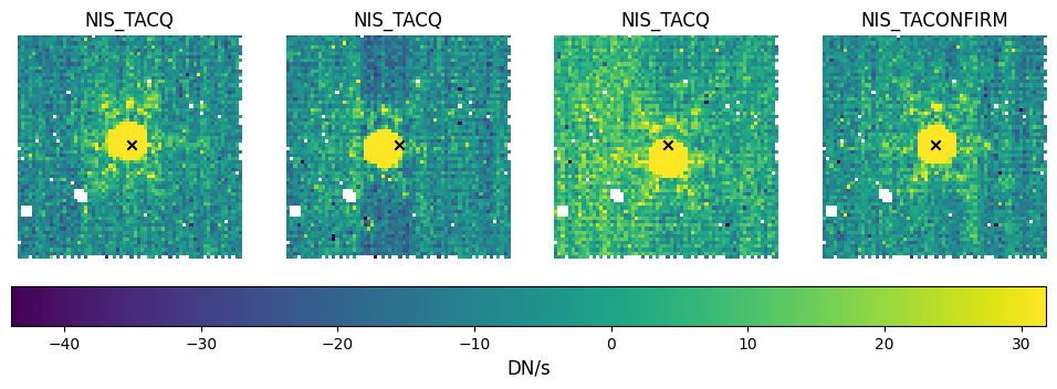
We can see that the source is being dithered in the first three images, and is nicely centered in the final image, as indicated by the black ‘x’ at the center of the array. The white pixels are those replaced by NaNs by the Detector1 pipeline due to saturation, outliers, or other data quality issues.
Examine Detector1 products#
We will begin by looking at the output of the first pipeline stage, the rateints files. As the 2D spectra over the duration of the time series will look very similar, we will only plot the first.
if doviz:
    display_soss_im(rateintsfiles[0])
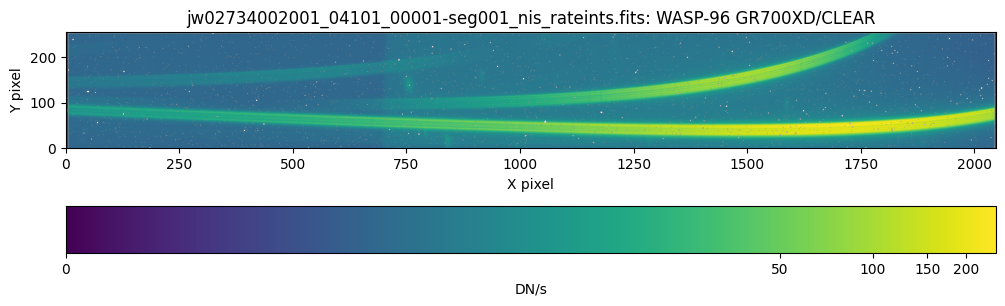
We are displaying these images on a logarithmic scale to be able to see the features of both the cross-dispersed spectral traces and the background. To see them on a linear scale, pass the argument lognormalize=False.
Orders 1, 2, and 3 are clearly visible in this image, along with some faint background sources. Order 1 extends across the full subarray and covers wavelengths from 0.9 $\mu m$ to 2.8 $\mu m$. The Order 2 trace, covering 0.6$ \mu m$ to 1.4$ \mu m$, overlaps with Order 1 at the longer-wavelength end of the traces. Order 3 peaks at ~0.6 $ \mu m$, though it is very faint.
For bright targets that would saturate the detector with the longer readout times of the SUBSTRIP256 subarray, users can elect to use the SUBSTRIP96 array. The 96-pixel vertical dimension of this subarray covers only the Order 1. For more information about the optics and spectral traces, see the GR700X grism documentation.
Although we did not extract a spectrum from it, it is interesting to look at the F277W spectral image:
if (doviz & (len(f277wfiles) > 0)):
    display_soss_im(f277wfiles[0])
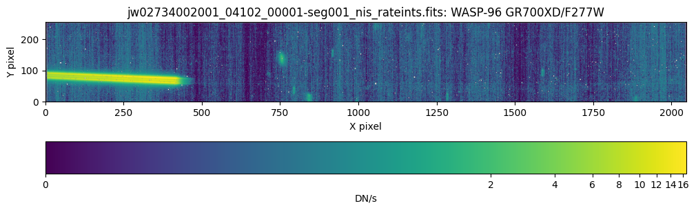
Compared to the CLEAR image above, we can clearly see that the Order 0 trace extends over only a small portion of the subarray, and Orders 2 and 3 are entirely absent. This is expected, because the left side of the subarray (in DMS orientation) corresponds to the longer wavelengths that SOSS is sensitive to, and the F277W filter covers only 2.413 $\mu m$ to 3.143 $\mu m$. This allows users to isolate the first order spectrum in the range where the first and second order overlap considerably.
We can also see several potentially contaminating zeroth-order sources in the image (the Order 0 for our target does not fall on the detector). Characterizing these sources in the F277W image can allow users to model and remove them in the full wavelength coverage spectra, although this capability is not currently included in the pipeline. Best practices for obtaining an F277W exposure are included in the SOSS Recommended Strategies.
The 1/f noise (vertical striping) is also more apparent in this exposure because of the lower signal relative to the background.
Examine Spec2 products#
Next we will look at the outputs of the second pipeline stage: the calibrated calints images and the preliminary x1dints extracted spectra. For more information about the structure and contents of these data products, see the documentation about x1d/x1dints and calints files.
if doviz:
    display_soss_im(calintsfiles[0])
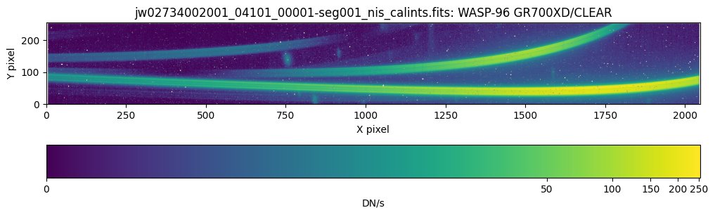
The SOSS sky background is characterized by a smooth rising gradient towards longer wavelengths, with a sharp discontinuity at around X=700 (corresponding to 2.1 $\mu m$ in Order 1) caused by the edges of the pick-off mirror (POM). The background varies with sky position and relative pointing due to the contribution of zodiacal light. Because of the variation in relative intensity on either side of the discontinuity, an empirical model cannot be simply linearly scaled to match a given observation. However, it is important to remove the background for most SOSS science use cases, so in the absence of a contemporaneous background exposure, the Spec2 bkg_subtract step finds the best match for each exposure from a library of empirical models scaled independently on either side of the discontinuity.
We can see that the background is considerably lower in the background-subtracted calints image compared to the previous rateints image, and the discontinuity is not as prominent, though some structure remains. The NIRISS team intends to continue improving the background subtraction algorithm in the future.
Now, let’s look at one of the extracted spectra.
if doviz:
    display_spectrum(x1d_spec2files[0], order=1)
Order 1 dimensions: 96 integrations, 2048 wavelengths
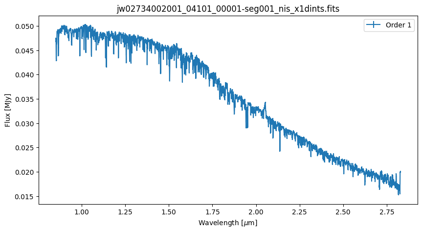
Note that not all of the “features” of this spectrum are absorption lines; many are due to bad pixels in the spectrum. As mentioned in the TSO3 Pipeline section, there is an optional pixel replacement step that may reduce this type of noise.
This is the first integration of the time series, but we are especially interested in how the spectrum changes over the duration of the observations. Let’s look at the spectrum as a function of both wavelength and time:
if doviz:
    spectrum_timeseries(x1d_spec2files)
Order 1 dimensions: 280 integrations, 2048 wavelengths
Order 2 dimensions: 280 integrations, 1783 wavelengths
/tmp/ipykernel_3291/2999729553.py:30: RuntimeWarning: Mean of empty slice
  first100 = np.nanmean(flux[:100, :], axis=0)
WARNING: Input data contains invalid values (NaNs or infs), which were automatically clipped. [astropy.stats.sigma_clipping]
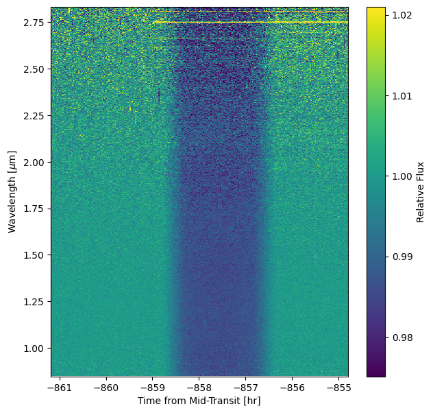
In this plot, the flux at each wavelength is normalized so that the decrease in flux caused by the transiting exoplanet is emphasized.
If we pass the argument normalize=False to the plotting function, the transit is much less obvious but we can see some interesting spectral features, as well as how the flux decreases at longer wavelengths.
if doviz:
    spectrum_timeseries(x1d_spec2files, normalize=False)
Order 1 dimensions: 280 integrations, 2048 wavelengths
Order 2 dimensions: 280 integrations, 1783 wavelengths
Examine TSO3 products#
Lastly, we will examine the products of the third and final pipeline stage: the final x1dints spectra and the white light (whtlt) curve for orders 1 and 2.
if doviz:
    display_spectrum(x1d_tso3file, order=1)
Order 1 dimensions: 280 integrations, 2048 wavelengths
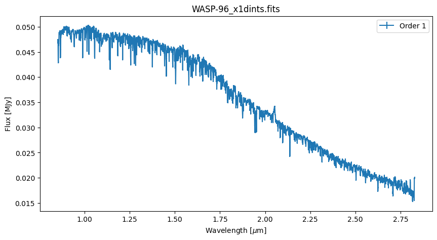
if doviz:
    display_spectrum(x1d_tso3file, order=2)
Order 2 dimensions: 280 integrations, 1783 wavelengths
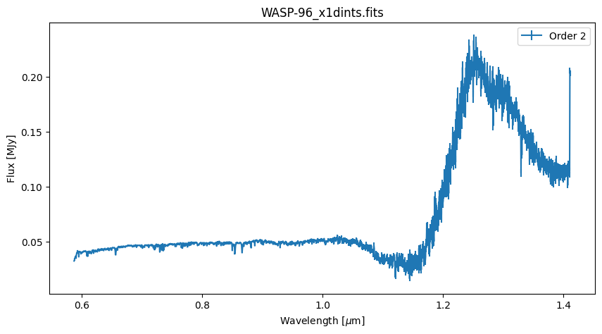
By eye, there is not much difference apparent between the Stage 2 x1dints files and the Stage 3 x1dints files; the main difference is that the outlier detection step has now been run. However, it is worth noting that in Order 2, measurements beyond ~1 $\mu m$ are not reliable due to contamination from Order 1.
We can also make the 2d transit plot again, using the final extracted spectrum:
if doviz:
    spectrum_timeseries(x1d_tso3file)
Order 1 dimensions: 280 integrations, 2048 wavelengths
Order 2 dimensions: 280 integrations, 1783 wavelengths
/tmp/ipykernel_3291/2999729553.py:30: RuntimeWarning: Mean of empty slice
  first100 = np.nanmean(flux[:100, :], axis=0)
WARNING: Input data contains invalid values (NaNs or infs), which were automatically clipped. [astropy.stats.sigma_clipping]
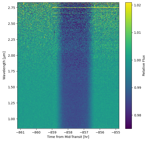
Lastly, let’s look at the white light curve. In this file, the flux at each wavelength has been summed to give us a single value at each timestamp.
We will plot the white light curve for orders 1 and 2, along with a simple transit model using the batman package (Kreidberg 2015). We adopt all of our planetary parameters from McGruder et al. 2023, except for the ratio of the planet radius to the stellar radius ($R_{p}/R_{*}$), which is from Kokori et al. 2023.
if doviz:
    # Set up the model parameters
    params = batman.TransitParams()
    params.t0 = 2456258.06272 - 2400000.5       # time of inferior conjunction
    params.per = 3.4252567                        # orbital period
    params.rp = 0.1175                            # planet radius (in units of stellar radii)
    params.a = 9.13                               # semi-major axis (in units of stellar radii)
    params.inc = 85.45                            # orbital inclination (in degrees)
    params.ecc = 0.                               # eccentricity
    params.w = 90.                                # longitude of periastron (in degrees)
    params.u = [0.16, 0.26]                       # limb darkening coefficients [u1, u2]
    params.limb_dark = "quadratic"                # limb darkening model

    # Display the light curves and models
    display_lightcurve(whtltfile, order=[1, 2], modelparams=params)
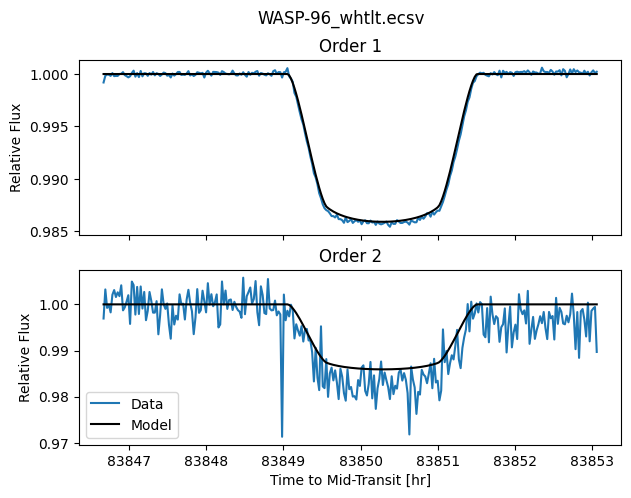
Since the model parameters were derived from a different reduction that used the same data, it makes sense that this model looks like a pretty good fit to the data by eye. Further model fitting is beyond the scope of this notebook, but can also be done using batman or a variety of other open-source software packages.
