Beginner: Searching MAST using astroquery.mast

Introduction and Goals:

This is a beginner tutorial on accessing the MAST Archive using the Astroquery API. We’ll cover the major search features you might find useful when querying for observations. By the end of this tutorial, you will:

• Understand how to search for observations hosted on the MAST Archive

• Download data products corresponding to your observations of interest

• Create a visual display of the downloaded data

Table of Contents

• Imports

• Three ways to search for MAST observations

  • By Region

  • By Object Name

  • By Criteria

• Getting Associated Data Products

  • Performing a Product Query

  • Filtering Data Products

• Downloading Products

• Displaying Data

• Further Reading

Imports

Let’s start by importing the packages we need for this notebook.

• astroquery.mast to access the MAST API

• astropy to create coordinate objects and access the data

• matplotlib to plot the data

from astropy.coordinates import SkyCoord
from astropy.io import fits
from astroquery.mast import Observations
from matplotlib.colors import SymLogNorm

import matplotlib.pyplot as plt

%matplotlib inline

Three Ways to Search for MAST Observations

1. By Region

To search by coordinates (and a radius), you can use query_region.

The coordinates can be given as a string or astropy.coordinates object, and the radius as a string or float object. If no radius is specified, the default is 0.2 degrees.

Let’s try an example search with the coordinates (322.49324, 12.16683) and no radius.

# This will give a warning that the coordinates are being interpreted as an ICRS coordinate provided in degrees
obsByRegion = Observations.query_region("322.49324 12.16683")
len(obsByRegion)

WARNING: InputWarning: Coordinate string is being interpreted as an ICRS coordinate provided in degrees. [astroquery.utils.commons]

12978

Excellent! At the time of writing, this search returns 2240 results. As the MAST archive grows, this number increases; you might see a larger value. Let’s take a look a subset of the results.

# Preview the first 3 results
obsByRegion[:3]

Table masked=True length=3

intentType	obs_collection	provenance_name	instrument_name	project	filters	wavelength_region	target_name	target_classification	obs_id	s_ra	s_dec	dataproduct_type	proposal_pi	calib_level	t_min	t_max	t_exptime	em_min	em_max	obs_title	t_obs_release	proposal_id	proposal_type	sequence_number	s_region	jpegURL	dataURL	dataRights	mtFlag	srcDen	obsid	distance
str11	str11	str31	str13	str12	str27	str16	str33	str56	str92	float64	float64	str10	str25	int64	float64	float64	float64	float64	float64	str106	float64	str20	str12	int64	str17043	str185	str186	str6	bool	float64	str9	float64
science	TESS	SPOC	Photometer	TESS	TESS	Optical	TESS FFI	--	tess-s0055-1-1	325.9351193555199	11.77496602082765	image	Ricker, George	3	59796.6013437963	59823.76825269676	475.199786	600.0	1000.0	--	59841.0	N/A	--	55	POLYGON 329.837843 19.006512 333.753586 8.161861 322.106193 4.225655 318.039501 15.437198 329.837843 19.006512	--	--	PUBLIC	False	nan	95133321	0.0
science	TESS	SPOC	Photometer	TESS	TESS	Optical	TESS FFI	--	tess-s0082-1-2	317.17154347395564	10.091041157822387	image	Ricker, George	3	60532.891556863426	60558.749996122686	158.399927	600.0	1000.0	--	60613.0	N/A	--	82	POLYGON 320.550581 17.936678 325.068597 6.875186 313.680238 2.326972 309.407072 13.006235 320.550581 17.936678	--	--	PUBLIC	False	nan	232881350	0.0
science	TESS	SPOC	Photometer	TESS	TESS	Optical	96703881	--	tess2022217014003-s0055-0000000096703881-0242-s	322.493171	12.166862	timeseries	Ricker, George	3	59796.60416888889	59823.76815293982	120.0	600.0	1000.0	--	59841.0	G04046	--	55	CIRCLE 322.493171 12.166862 0.00138889	--	mast:TESS/product/tess2022217014003-s0055-0000000096703881-0242-s_lc.fits	PUBLIC	False	nan	93770500	0.0

The columns of the above table (there are many!) correspond to searchable fields in the MAST database. You can find the full list of criteria here and an example of performing a search by criteria down below.

If we want to avoid that pesky warning from the search above we can create a coordinates object and pass it to our search. Let’s try that now, and in addition, let’s add a radius of 1 arcsecond to this search.

# Set up our coordinates object
coord = SkyCoord(290.213503, -11.800746, unit='deg')

# Same search as above, now with a radius of 1 arcsecond
obsByRegion2 = Observations.query_region(coord, radius='1s')
len(obsByRegion2)

11

Sanity check: we expect that as the radius gets smaller, we get fewer results. In this case, only 15 results are returned.

Let’s take a look at the results again, but let’s limit the columns that get displayed.

# Let's limit the number of columns we see at once
columns = ['obs_collection', 'intentType', 'instrument_name', 
           'target_name', 't_exptime', 'filters', 'dataproduct_type']

# Show the results with the above columns only
obsByRegion2[columns]

Table length=11

obs_collection	intentType	instrument_name	target_name	t_exptime	filters	dataproduct_type
str5	str7	str10	str12	float64	str4	str5
TESS	science	Photometer	TESS FFI	475.199781	TESS	image
TESS	science	Photometer	TESS FFI	158.399925	TESS	image
PS1	science	GPC1	1126.007	731.0	g	image
PS1	science	GPC1	1126.007	900.0	i	image
PS1	science	GPC1	1126.007	876.0	r	image
PS1	science	GPC1	1126.007	580.0	y	image
PS1	science	GPC1	1126.007	480.0	z	image
HLSP	science	Photometer	TICA FFI	475.2	TESS	image
HLSP	science	Photometer	TICA FFI	158.4	TESS	image
GALEX	science	GALEX	AIS_246_1_35	176.0	NUV	image
GALEX	science	GALEX	AIS_246_1_35	176.0	FUV	image

This “streamlined” view is helpful: it avoids visual clutter and helps you to focus on the fields that are most relevant to your search.

2. By Object Name

To search for an object by name, you can use the query.object function. This function also optionally allows you to specify a radius.

The object name is first resolved to coordinates by a call to the Simbad and NED archives. Then, the search proceeeds based on these coordinates.

obsByName = Observations.query_object("M51", radius=".005 deg")

print("Number of results:", len(obsByName))

obsByName[:5]

Number of results: 7503

Table masked=True length=5

intentType	obs_collection	provenance_name	instrument_name	project	filters	wavelength_region	target_name	target_classification	obs_id	s_ra	s_dec	dataproduct_type	proposal_pi	calib_level	t_min	t_max	t_exptime	em_min	em_max	obs_title	t_obs_release	proposal_id	proposal_type	sequence_number	s_region	jpegURL	dataURL	dataRights	mtFlag	srcDen	obsid	distance
str11	str11	str31	str12	str13	str26	str19	str64	str49	str53	float64	float64	str10	str23	int64	float64	float64	float64	float64	float64	str107	float64	str16	str13	int64	str17792	str175	str176	str6	bool	float64	str9	float64
science	TESS	SPOC	Photometer	TESS	TESS	Optical	TESS FFI	--	tess-s0016-4-3	200.6066940322731	50.01251405441704	image	Ricker, George	3	58738.14190212	58762.80885051	1425.599358	600.0	1000.0	--	58782.3333334	N/A	--	16	POLYGON 188.96005900 47.31461100 195.80207500 58.03466100 213.76319300 51.45788000 203.63432700 41.78187500 188.96005900 47.31461100	--	--	PUBLIC	False	nan	27545566	0.0
science	TESS	SPOC	Photometer	TESS	TESS	Optical	TESS FFI	--	tess-s0022-2-1	198.24826184396446	45.21473093959813	image	Ricker, George	3	58898.81559378	58925.98257992	1425.599393	600.0	1000.0	--	58945.0	N/A	--	22	POLYGON 209.81203800 45.13366400 199.37165100 36.75577700 186.47721200 44.07435900 197.22646800 53.68842400 209.81203800 45.13366400	--	--	PUBLIC	False	nan	27347170	0.0
science	TESS	SPOC	Photometer	TESS	TESS	Optical	TESS FFI	--	tess-s0023-2-2	206.11364361798434	41.534991636349474	image	Ricker, George	3	58927.60756876	58954.37813731	1425.599383	600.0	1000.0	--	58973.0	N/A	--	23	POLYGON 217.19928400 43.86714800 209.71103500 33.48941000 195.67778400 38.51512800 201.79979000 49.12765700 217.19928400 43.86714800	--	--	PUBLIC	False	nan	27386992	0.0
science	TESS	SPOC	Photometer	TESS	TESS	Optical	TESS FFI	--	tess-s0049-2-1	204.06913817292593	42.4477011962157	image	Ricker, George	3	59636.975013854164	59663.81560847222	475.199787	600.0	1000.0	--	59695.0	N/A	--	49	POLYGON 215.129288 42.6299 205.417683 34.012968 192.868429 41.149492 202.762088 50.900239 215.129288 42.6299	--	--	PUBLIC	False	nan	83163378	0.0
science	TESS	SPOC	Photometer	TESS	TESS	Optical	TESS FFI	--	tess-s0076-1-1	209.07126289767237	46.689635318292865	image	Ricker, George	3	60367.19414883102	60394.280102627316	158.399923	600.0	1000.0	--	60438.0	N/A	--	76	POLYGON 220.895636 46.249072 209.783858 38.201258 196.899205 45.853449 208.607539 55.186936 220.895636 46.249072	--	--	PUBLIC	False	nan	214650609	0.0

For some special catalogs, like those used with Kepler, K2, and TESS, astroquery performs a direct lookup using the MAST catalog. It is important to include both the catalog identifier and number when searching one of these datasets; for example, to query the TESS Input catalog you would use “TIC 261136679”, rather than a plain “261136679”.

obsByTessName = Observations.query_object("TIC 261136679", radius="1s")

# As before, we use columns to limit the display
columns = ['obs_collection', 'wavelength_region', 'provenance_name', 't_min', 't_max', 'obsid']
obsByTessName[columns][:10]

Table length=10

obs_collection	wavelength_region	provenance_name	t_min	t_max	obsid
str11	str10	str17	float64	float64	str9
TESS	Optical	SPOC	58324.81304390046	58352.666903854166	60865631
TESS	Optical	SPOC	58410.41593530092	58436.33232072917	61132377
TESS	Optical	SPOC	58516.85312458334	58541.49921487269	62468248
TESS	Optical	SPOC	58596.27096596065	58623.37541814815	65153352
TESS	Optical	SPOC	58624.45954434028	58652.37651001157	65180725
TESS	Optical	SPOC	58653.41816987268	58681.85536055556	65462606
TESS	Optical	SPOC	59035.7791077	59060.13994723	27797249
TESS	Optical	SPOC	59061.34744424	59086.59716169	27844486
TESS	Optical	SPOC	59144.0128561	59169.44312553	28131771
TESS	Optical	SPOC	59228.2486492	59253.56140963	28364165

It’s worth noting that even though we queried using the TESS Input Catalog, not all of the results are from the TESS mission. The TIC is a catalog like any other, and the MAST Archive resolves the input name to a location on the sky. Other missions that have observed the same region will also return results.

To search for results that are specific to TESS, or your mission of choice, see the ‘by other criteria’ section below.

3. By Other Criteria (with or without name/region)

To search for observations based on additonal parameters, you can use query_criteria. In a sense, this is a more powerful version of the tools above, as you can still search by coordinates and objectname; however, you can inculde additional desired criteria. You may also run the search without specifying a name or coordinates.

To perform the search, give your critera as keyword arguments. Valid criteria and their descriptions are listed here. (Note that these are columns of the results tables we saw above!) Some relevant examples are: “filters”, “t_exptime” (exposure time), instrument_name, “provenance_name”, and “sequence_number”.

Let’s for TESS Sector 9 data with an exposure time between 1400 and 1500s.

obsByCriteria = Observations.query_criteria(obs_collection=["TESS"], sequence_number=9,
                                            t_exptime=[1400, 1500])

columns = ['target_name', 's_ra', 's_dec', 't_exptime', 'obsid']
obsByCriteria[columns][:5]

Table length=5

target_name	s_ra	s_dec	t_exptime	obsid
str8	float64	float64	float64	str8
TESS FFI	148.8381670809981	-53.640196587551905	1425.599414	62895676
TESS FFI	162.4696250638618	-5.425652707919927	1425.599414	62892977
TESS FFI	151.37494470193366	-26.74595469529746	1425.599414	62895165
TESS FFI	173.83652057983417	-10.27752013936934	1425.599414	62892431
TESS FFI	169.0707180032819	-21.387226979894706	1425.599414	62891912

There’s no limit on the number of filters you can apply in a search. It may be an interesting exercise for the reader to go through the example below and figure out what exactly we’re searching for.

(Hint: check the field descriptions)

# Make sure to run this cell, as the data is used in the sections that follow

exByCriteria = Observations.query_criteria(obs_collection=["HLA"], s_dec=[50, 60], 
                                           calib_level=[3], proposal_pi="Mould*", 
                                           dataproduct_type="IMAGE", t_max=[49800, 49820])

columns = ['obs_collection', 'obs_id', 'target_name', 'filters', 'instrument_name', 'proposal_id']
exByCriteria[columns]

Table length=4

obs_collection	obs_id	target_name	filters	instrument_name	proposal_id
str3	str27	str12	str9	str9	str4
HLA	hst_05766_04_wfpc2_f555w_pc	NGC5457-FLD2	F555W	WFPC2/PC	5766
HLA	hst_05766_04_wfpc2_f555w_wf	NGC5457-FLD2	F555W	WFPC2/WFC	5766
HLA	hst_05766_04_wfpc2_total_pc	NGC5457-FLD2	DETECTION	WFPC2/PC	5766
HLA	hst_05766_04_wfpc2_total_wf	NGC5457-FLD2	DETECTION	WFPC2/WFC	5766

Getting Associated Data Products

Performing a Product Query

Each observation returned from a MAST query can have one or more associated data products. For example, a JWST observation might return an uncalibrated file, a guide-star file, and the science data you’re searching for.

You can input a table of observations or list of observation ids (“obs_id”) and get_product_list will return a table containing the associated data products.

Since we already have a list of observations, we can use that as the starting point for our query. To keep it simple, let’s look at only the last observation from our search above.

# Let's select a small subset from our critera search above
newObsList = exByCriteria[-1:]

# Now we get the list of products associated with that observation
dataProducts = Observations.get_product_list(newObsList)

dataProducts[:5]

Table masked=True length=5

obsID	obs_collection	dataproduct_type	obs_id	description	type	dataURI	productType	productGroupDescription	productSubGroupDescription	productDocumentationURL	project	prvversion	proposal_id	productFilename	size	parent_obsid	dataRights	calib_level	filters
str8	str3	str5	str30	str67	str1	str96	str9	str28	str8	str1	str8	str19	str4	str43	int64	str8	str6	int64	str9
25153181	HLA	image	hst_05766_04_wfpc2_f555w_wf_02	Preview-Full	S	mast:HLA/url/cgi-bin/preview.cgi?dataset=hst_05766_04_wfpc2_f555w_wf_02	PREVIEW	--	--	--	HLA	--	5766	hst_05766_04_wfpc2_f555w_wf_02_drz.jpg	--	25579950	PUBLIC	2	F555W
25153181	HLA	image	hst_05766_04_wfpc2_f555w_wf_02	HLA simple fits science image	S	mast:HLA/url/cgi-bin/getdata.cgi?dataset=hst_05766_04_wfpc2_f555w_wf_02_drz.fits	SCIENCE	--	DRZ	--	HLA	--	5766	hst_05766_04_wfpc2_f555w_wf_02_drz.fits	10281600	25579950	PUBLIC	2	F555W
25579950	HLA	image	hst_05766_04_wfpc2_total_wf	Preview-Full	C	mast:HLA/url/cgi-bin/preview.cgi?dataset=hst_05766_04_wfpc2_total_wf	PREVIEW	--	--	--	HLA	--	5766	hst_05766_04_wfpc2_total_wf_drz.jpg	--	25579950	PUBLIC	3	DETECTION
25579950	HLA	image	hst_05766_04_wfpc2_total_wf	HLA DAOPHOT Catalog	C	mast:HLA/url/cgi-bin/getdata.cgi?download=1&filename=hst_05766_04_wfpc2_total_wf_daophot_trm.cat	SCIENCE	Minimum Recommended Products	DAOPHOT	--	HLA	--	5766	hst_05766_04_wfpc2_total_wf_daophot_trm.cat	--	25579950	PUBLIC	3	DETECTION
25579950	HLA	image	hst_05766_04_wfpc2_total_wf	HLA simple fits science image	C	mast:HLA/url/cgi-bin/getdata.cgi?dataset=hst_05766_04_wfpc2_total_wf_drz.fits	SCIENCE	Minimum Recommended Products	DRZ	--	HLA	--	5766	hst_05766_04_wfpc2_total_wf_drz.fits	30798720	25579950	PUBLIC	3	DETECTION

Filtering the Data Products

After the data products have been retrieved, you can use filter_products to download only data products that meet your given criteria. Available filters are listed here. Some examples are: “mrp_only” (Minimum Recommended Products) and “extension” (file extension).

A note on filtering: each listed filter is joined with an AND, but each option within that filter is joined with an OR. For example, the search below will return any products that are ‘science’ type and have a calibration level of 2 or 3.

scienceProducts = Observations.filter_products(dataProducts, productType=["SCIENCE"],
                                               calib_level=[2, 3], mrp_only=False)

scienceProducts[:5]

Table masked=True length=5

obsID	obs_collection	dataproduct_type	obs_id	description	type	dataURI	productType	productGroupDescription	productSubGroupDescription	productDocumentationURL	project	prvversion	proposal_id	productFilename	size	parent_obsid	dataRights	calib_level	filters
str8	str3	str5	str30	str67	str1	str96	str9	str28	str8	str1	str8	str19	str4	str43	int64	str8	str6	int64	str9
25153181	HLA	image	hst_05766_04_wfpc2_f555w_wf_02	HLA simple fits science image	S	mast:HLA/url/cgi-bin/getdata.cgi?dataset=hst_05766_04_wfpc2_f555w_wf_02_drz.fits	SCIENCE	--	DRZ	--	HLA	--	5766	hst_05766_04_wfpc2_f555w_wf_02_drz.fits	10281600	25579950	PUBLIC	2	F555W
25579950	HLA	image	hst_05766_04_wfpc2_total_wf	HLA DAOPHOT Catalog	C	mast:HLA/url/cgi-bin/getdata.cgi?download=1&filename=hst_05766_04_wfpc2_total_wf_daophot_trm.cat	SCIENCE	Minimum Recommended Products	DAOPHOT	--	HLA	--	5766	hst_05766_04_wfpc2_total_wf_daophot_trm.cat	--	25579950	PUBLIC	3	DETECTION
25579950	HLA	image	hst_05766_04_wfpc2_total_wf	HLA simple fits science image	C	mast:HLA/url/cgi-bin/getdata.cgi?dataset=hst_05766_04_wfpc2_total_wf_drz.fits	SCIENCE	Minimum Recommended Products	DRZ	--	HLA	--	5766	hst_05766_04_wfpc2_total_wf_drz.fits	30798720	25579950	PUBLIC	3	DETECTION
25579950	HLA	image	hst_05766_04_wfpc2_total_wf	HLA SExtractor Catalog	C	mast:HLA/url/cgi-bin/getdata.cgi?download=1&filename=hst_05766_04_wfpc2_total_wf_sexphot_trm.cat	SCIENCE	Minimum Recommended Products	SEXPHOT	--	HLA	--	5766	hst_05766_04_wfpc2_total_wf_sexphot_trm.cat	--	25579950	PUBLIC	3	DETECTION
24556184	HST	image	u2ms0402t	DADS C0F file - Calibrated exposure WFPC/WFPC2/FOC/FOS/GHRS/HSP	S	mast:HST/product/u2ms0402t_c0f.fits	SCIENCE	--	C0F	--	CALWFPC2	2.5.3 (Sep 4, 2008)	5766	u2ms0402t_c0f.fits	10307520	25579950	PUBLIC	2	F555W

Downloading Products

Passing a table of products (like the one above) to download_products will download the entire table. You can also pass a list of Observation IDs (obs_id) if you know them.

download_products also allows you to filter data as you request the download. In the example below, we will only download the drizzled files (drz.fits).

Products will by default be downloaded into the current working directory, in a subdirectory called “mastDownload.”
The full local file paths will have the form “mastDownload/Mission/Observation ID/file.”

# This is the filtered download of the scienceProducts table
manifest = Observations.download_products(scienceProducts, extension=("drz.fits"))

# Uncomment below for "plain" download of the scienceProducts table
# manifest = Observations.download_products(scienceProducts)

Downloading URL https://mast.stsci.edu/api/v0.1/Download/file?uri=mast:HLA/url/cgi-bin/getdata.cgi?dataset=hst_05766_04_wfpc2_f555w_wf_02_drz.fits to ./mastDownload/HLA/hst_05766_04_wfpc2_f555w_wf_02/hst_05766_04_wfpc2_f555w_wf_02_drz.fits ...

 [Done]

Downloading URL https://mast.stsci.edu/api/v0.1/Download/file?uri=mast:HLA/url/cgi-bin/getdata.cgi?dataset=hst_05766_04_wfpc2_total_wf_drz.fits to ./mastDownload/HLA/hst_05766_04_wfpc2_total_wf/hst_05766_04_wfpc2_total_wf_drz.fits ...

 [Done]

Note: download_products includes caching by default. If you have downloaded the files before, they will not be downloaded again unless caching is turned off. This may cause issues if the data is updated and the filename remains the same!

manifest

Table length=2

Local Path	Status	Message	URL
str89	str8	object	object
./mastDownload/HLA/hst_05766_04_wfpc2_f555w_wf_02/hst_05766_04_wfpc2_f555w_wf_02_drz.fits	COMPLETE	None	None
./mastDownload/HLA/hst_05766_04_wfpc2_total_wf/hst_05766_04_wfpc2_total_wf_drz.fits	COMPLETE	None	None

The manifest returns useful information about the status of the files. You can find the local path, along with a status. This will either be COMPLETE, SKIPPED, or ERROR. If the status is ERROR, there will be additional information in the ‘Message’ column. The URL field includes a link to directly download the data.

Displaying Data

At this point the data is ready for analysis, and we are done querying the MAST Archive.

Below we take a look at the data files using astropy.fits and matplotlib.

# Get the filenames from the manifest
filename0 = manifest['Local Path'][0]
filename1 = manifest['Local Path'][1]

# Open the files using astropy.fits
file1 = fits.open(filename0)
file2 = fits.open(filename1)

f, (ax1, ax2) = plt.subplots(1, 2)
f.set_figheight(5)
f.set_figwidth(12)
ax1.imshow(file1[0].data, cmap="inferno", norm=SymLogNorm(linthresh=0.03, vmin=0, vmax=1.5))
ax2.imshow(file2['SCI'].data, cmap="inferno", norm=SymLogNorm(linthresh=0.03, vmin=-0.01, vmax=1.5))

<matplotlib.image.AxesImage at 0x7f0f28508850>

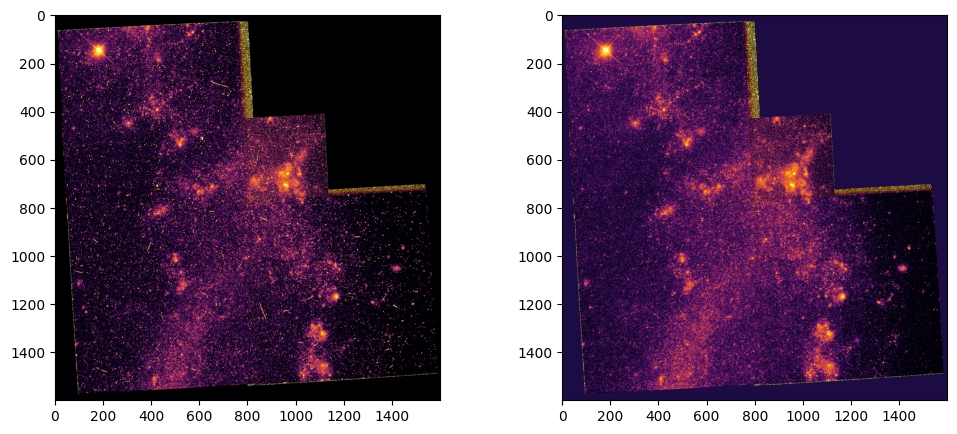
We see the same region of the sky, with subtle differences caused by the differing filters.

Further Reading

Full documentation on astroquery.mast can be found here.

About this Notebook

For additonal questions, comments, or feedback, please email archive@stsci.edu.

Authors: Thomas Dutkiewicz, Scott Fleming
Keywords: MAST, astroquery
Latest update Oct 2022
Next Review: Apr 2023

Top of Page