Hubble Source Catalog SWEEPS Proper Motion Notebook

2019 - 2022, Steve Lubow, Rick White, Trenton McKinney

This notebook shows how to access the new proper motions available for the SWEEPS field in version 3.1 of the Hubble Source Catalog. Data tables in MAST CasJobs are queried from Python using the mastcasjobs module. Additional information is available on the SWEEPS Proper Motions help page.

Instructions:

• Complete the initialization steps described below.

• Run the notebook to completion.

• Modify and rerun any sections of the Table of Contents below.

Running the notebook from top to bottom takes about 7 minutes (depending on the speed of your computer).

Table of Contents

• Intialization

• Properties of Full Catalog

  • Sky Coverage

  • Proper Motion Distributions

  • Visit Distribution

  • Time Coverage Distributions

  • Magnitude Distributions

  • Color Magnitude Diagram

  • Detection Positions

• Good Photometric Objects

• Science Applications

  • Proper Motions on the CMD

  • Proper Motions in Bulge Versus Disk

  • White Dwarfs

  • QSO Candidates

  • High Proper Motion Objects

  • HLA Cutout Images for Selected Objects

Initialization

Install Python modules

1. This notebook requires the use of Python 3.

2. Modules can be installed with conda, if using the Anaconda distribution of python, or with pip.

   • If you are using conda, do not install / update / remove a module with pip, that exists in a conda channel.

   • If a module is not available with conda, then it’s okay to install it with pip

3. Install mastcasjobs and casjobs with pip:

pip install mastcasjobs

Set up your CasJobs account information

You must have a MAST Casjobs account. Note that MAST Casjobs accounts are independent of SDSS Casjobs accounts.

For easy startup, you can optionally set the environment variables CASJOBS_USERID and/or CASJOBS_PW with your Casjobs account information. The Casjobs user ID and password are what you enter when logging into Casjobs.

This script prompts for your Casjobs user ID and password during initialization if the environment variables are not defined.

import astropy
import time
import sys
import os
import requests
import numpy as np
import matplotlib.pyplot as plt
import matplotlib.gridspec as gridspec
from matplotlib.colors import LogNorm
from pathlib import Path

# check that version of mastcasjobs is new enough
# we are using some features not in version 0.0.1
from pkg_resources import get_distribution
from packaging.version import Version as V

assert V(get_distribution("mastcasjobs").version) >= V('0.0.2'), """
A newer version of mastcasjobs is required.
Update mastcasjobs to current version using this command:
pip install --upgrade git+git://github.com/rlwastro/mastcasjobs@master
"""

import mastcasjobs

from PIL import Image
from io import BytesIO

## For handling ordinary astropy Tables
from astropy.table import Table
from astropy.io import fits, ascii

from fastkde import fastKDE
from scipy.interpolate import RectBivariateSpline
from astropy.modeling import models, fitting

# There are a number of relatively unimportant warnings that 
# show up, so for now, suppress them:
import warnings
warnings.filterwarnings("ignore")

# set width for pprint
astropy.conf.max_width = 150

/tmp/ipykernel_2008/609964975.py:14: DeprecationWarning: pkg_resources is deprecated as an API. See https://setuptools.pypa.io/en/latest/pkg_resources.html
  from pkg_resources import get_distribution

# set universal matplotlib parameters
plt.rcParams.update({'font.size': 16})

HSCContext = "HSCv3"

Set up Casjobs environment.

import getpass
if not os.environ.get('CASJOBS_USERID'):
    os.environ['CASJOBS_USERID'] = input('Enter Casjobs UserID:')
if not os.environ.get('CASJOBS_PW'):
    os.environ['CASJOBS_PW'] = getpass.getpass('Enter Casjobs password:')

Create table in MyDB with selected SWEEPS objects

Note that the query restricts the sample to matches with at least 10 detections in each of F606W and F814W. This can be modified depending on the science goals.

This uses an existing MyDB.SWEEPS table if it already exists in your CasJobs account. If you want to change the query, either change the name of the output table or drop the table to force it to be recreated. Usually the query completes in about a minute, but if the database server is heavily loaded then it can take much longer.

DBtable = "SWEEPS"
jobs = mastcasjobs.MastCasJobs(context="MyDB")

try:
    print(f"Retrieving table MyDB.{DBtable} (if it exists)")
    tab = jobs.fast_table(DBtable, verbose=True)
except ValueError:
    print(f"Table MyDB.{DBtable} not found, running query to create it")

    # drop table if it already exists
    jobs.drop_table_if_exists(DBtable)

    # get main information
    query = f"""
        select a.ObjID,  RA=a.raMean, Dec=a.decMean, RAerr=a.raMeanErr, Decerr=a.decMeanErr,
            c.NumFilters, c.NumVisits,
            a_f606w=i1.MagMed,  a_f606w_n=i1.n, a_f606w_mad=i1.MagMAD,
            a_f814w=i2.MagMed, a_f814w_n=i2.n, a_f814w_mad=i2.MagMAD,
            bpm=a.pmLat, lpm=a.pmLon, bpmerr=a.pmLatErr, lpmerr=a.pmLonErr,
            pmdev=sqrt(pmLonDev*pmLonDev+pmLatDev*pmLatDev),
            yr=(a.epochMean - 47892)/365.25+1990, 
            dT=(a.epochEnd-a.epochStart)/365.25,
            yrStart=(a.epochStart - 47892)/365.25+1990,
            yrEnd=(a.epochEnd - 47892)/365.25+1990
        into mydb.{DBtable}
        from AstromProperMotions a join AstromSumMagAper2 i1 on 
             i1.ObjID=a.ObjID and i1.n >=10 and i1.filter ='F606W' and i1.detector='ACS/WFC'
         join AstromSumMagAper2 i2 on 
             i2.ObjID=a.ObjID and i2.n >=10 and i2.filter ='F814W' and i2.detector='ACS/WFC'
         join AstromSumPropMagAper2Cat c on a.ObjID=c.ObjID
    """

    t0 = time.time()
    jobid = jobs.submit(query, task_name="SWEEPS", context=HSCContext)
    print("jobid=", jobid)
    results = jobs.monitor(jobid)
    print(f"Completed in {(time.time()-t0):.1f} sec")
    print(results)

    # slower version using CasJobs output queue
    # tab = jobs.get_table(DBtable, verbose=False)
    
    # fast version using special MAST Casjobs service
    tab = jobs.fast_table(DBtable, verbose=True)

Retrieving table MyDB.SWEEPS (if it exists)

13.2 s: Retrieved 157.86MB table MyDB.SWEEPS

19.4 s: Converted to 443932 row table

tab

Table length=443932

ObjID	RA	Dec	RAerr	Decerr	NumFilters	NumVisits	a_f606w	a_f606w_n	a_f606w_mad	a_f814w	a_f814w_n	a_f814w_mad	bpm	lpm	bpmerr	lpmerr	pmdev	yr	dT	yrStart	yrEnd
int64	float64	float64	float64	float64	int32	int32	float64	int32	float64	float64	int32	float64	float64	float64	float64	float64	float64	float64	float64	float64	float64
4000709002286	269.7911379669984	-29.206156187411423	0.6964818624528099	0.2730062330800141	2	47	22.127399444580078	47	0.021600723266601562	21.13010025024414	47	0.0167999267578125	2.087558644949346	-7.738272329430371	0.38854582276386007	0.22115673368981237	2.887154518133692	2013.3007902147058	11.371914541371764	2003.4361796620085	2014.8080942033803
4000709002287	269.7955922590832	-29.206151631494986	0.24020216760386343	0.18524811391217816	2	47	21.508499145507812	47	0.029998779296875	20.69930076599121	47	0.023900985717773438	-2.8930568503344967	-0.7898583846555245	0.1316584790053578	0.12462185695877996	1.474676632663785	2013.3007902147058	11.371914541371764	2003.4361796620085	2014.8080942033803
4000709002288	269.81608933789283	-29.206155196641195	0.3040684131020671	0.2850407586200256	2	47	21.654399871826172	47	0.03650093078613281	20.85770034790039	47	0.017101287841796875	4.65866649193795	-3.2098804580343785	0.13931172183651183	0.20648097604781626	1.9570357322713463	2013.3007902147058	11.371914541371764	2003.4361796620085	2014.8080942033803
4000709002289	269.8259694163096	-29.20615668840751	0.3564325426522067	0.39542200297333663	2	47	19.79170036315918	47	0.028200149536132812	19.06909942626953	47	0.019300460815429688	-0.45662407290928664	-2.0909050045433832	0.15758175952333653	0.2763881282194908	2.2415238499377685	2013.3007902147058	11.371914541371764	2003.4361796620085	2014.8080942033803
4000709002290	269.83486415728754	-29.206155266983643	0.16299639839198538	0.14062839407811836	2	46	20.566649436950684	46	0.015949249267578125	19.847750663757324	46	0.014801025390625	4.459275526783969	-2.0433632344343886	0.17899727943855331	0.18503594468835396	1.0091970907052557	2013.5152382701992	3.0067822490178155	2011.8013119543625	2014.8080942033803
4000709002291	269.83512411344606	-29.2061635244798	0.18282583105108072	0.2093503650681541	2	46	20.17770004272461	46	0.028949737548828125	19.489749908447266	46	0.03639984130859375	4.090870144734149	-8.059473158394072	0.20446351152189052	0.26206212529696193	1.293050027027329	2013.5152382701992	3.0067822490178155	2011.8013119543625	2014.8080942033803
4000709002292	269.7964913295107	-29.20618734483311	0.30491102397226527	0.26784496777851086	2	47	20.83639907836914	47	0.02239990234375	20.088300704956055	47	0.02230072021484375	-1.7001866534338244	-5.963967462759159	0.14814161799844547	0.1920517681653374	1.9671761489287654	2013.3007902147058	11.371914541371764	2003.4361796620085	2014.8080942033803
4000709002293	269.7872745304419	-29.206257828852337	1.351885504360048	1.0460614189471378	2	46	25.99174976348877	46	0.0852499008178711	24.204350471496582	46	0.05684947967529297	-2.290436263458843	-9.596838559623627	0.779373480816473	0.6485354032580087	8.518045574208871	2013.3206150152016	11.371914541371764	2003.4361796620085	2014.8080942033803
4000709002294	269.80888716219647	-29.206189189626002	1.4134596118752103	1.2518047802862953	2	47	25.465349197387695	46	0.08104991912841797	23.27630043029785	47	0.032100677490234375	4.381302303073221	-4.701855876394848	0.4784428793001857	1.0219363775325352	6.469654565147953	2013.3007902147058	11.371914541371764	2003.4361796620085	2014.8080942033803
4000709002295	269.8234425365187	-29.206188473661626	0.35597857562160923	1.5877104410672558	2	36	24.13195037841797	36	0.04940032958984375	23.0174503326416	36	0.038100242614746094	4.48015296877619	-8.000985108228505	0.5070876244065738	0.7286553380951986	4.141157872026995	2013.174250263767	11.298715372835678	2003.4361796620085	2014.7348950348442
...	...	...	...	...	...	...	...	...	...	...	...	...	...	...	...	...	...	...	...	...	...
4000946339500	269.6899686412092	-29.27697845186784	1.7581744127758168	0.9354091074080774	2	10	23.770350456237793	10	0.06089973449707031	22.6496000289917	10	0.037400245666503906	-4.433870501660679	-1.6701167031929542	2.2930714454340286	1.3766459346536568	4.298430412355294	2013.9000436508227	2.1913492111623043	2012.4990161054518	2014.6903653166141
4000946380565	269.71004704275265	-29.258318619418723	1.4337273570795164	1.471655230308599	2	11	23.99720001220703	11	0.03730010986328125	22.51849937438965	11	0.020000457763671875	1.6111158133637464	-6.745663286831152	1.9631691651841359	1.720280363564143	4.409524084435339	2013.9002540765803	2.3094412747548714	2012.4990161054518	2014.8084573802066
4000946404892	269.67530078168915	-29.247162734242675	1.3763906949106726	1.6133894601395353	2	12	24.929399490356445	12	0.02920055389404297	23.21535015106201	12	0.06190013885498047	-4.240018447223827	-5.301395921474695	2.3240489286645727	2.4646517810785467	5.034040969645841	2013.3725317320211	2.0458630494273624	2012.389031376682	2014.4348944261094
4000946417296	269.7016328152704	-29.246070466593743	3.130830982636958	3.185144112877607	2	11	25.600500106811523	11	0.23419952392578125	24.028099060058594	11	0.2503986358642578	0.3265864932598421	-6.491394647992156	6.396715459697641	2.5782652825923047	8.829447098663028	2013.7731122440448	2.01948620036275	2012.6708791162512	2014.6903653166141
4000949430259	269.722986295747	-29.21197112017265	1.361963963773738	1.158905612896655	3	15	24.502249717712402	14	0.06614971160888672	23.928850173950195	14	0.056850433349609375	4.745787093281551	-3.4149224348359475	0.9875243981622149	0.6006686739150457	5.081087460494774	2004.567449081762	6.212572361916957	2004.14378291216	2010.356355274077
4000949692413	269.847657491686	-29.213464437142868	2.3678034671958668	2.0224597819540673	2	10	24.422550201416016	10	0.11170005798339844	22.581549644470215	10	0.0209503173828125	1.6834992526734194	-14.490467506156065	3.4740642144508795	4.492656398011582	5.946113188318635	2013.955340339603	1.5098539308761485	2013.2982402725042	2014.8080942033803
4000949719295	269.8230388680129	-29.20072120181885	6.9256239011552925	2.49884610751816	2	10	25.977850914001465	10	0.10779953002929688	24.156999588012695	10	0.03194999694824219	-0.009307948981069264	-9.255580848582802	1.8581178329802082	1.5241924426465314	15.473545552827103	2012.4700600740625	10.768784408135662	2003.4361796620085	2014.2049640701443
4000979902333	269.804403240861	-29.192813265455396	2.3859956776447127	1.392848515948042	2	10	25.71024990081787	10	0.06535053253173828	24.112099647521973	10	0.05470085144042969	0.7550276872362829	-4.7745907025067345	3.6257686130953477	1.461781567688497	5.065034698466592	2013.6589915119716	2.5308665509739208	2012.2040284838704	2014.7348950348442
4000979908546	269.8156665822647	-29.189854516331526	0.9143748593616481	2.1238192007085037	2	12	25.4466495513916	12	0.15910053253173828	23.336549758911133	12	0.06319999694824219	-7.2055855532918205	-9.683292833608878	2.618264686941967	3.0724808097663883	5.246267309545055	2013.8340336110703	1.6017431136587867	2013.2063510897215	2014.8080942033803
4000980227788	269.7998513044728	-29.19707771926519	1.8494859814888565	1.5991491655370784	2	12	24.400450706481934	12	0.10389995574951172	22.93809986114502	12	0.02064990997314453	0.15278595605010709	-7.172152518535961	0.691934557090257	0.49373163797911374	5.7619744099400085	2012.6568721424214	11.371914541371764	2003.4361796620085	2014.8080942033803

Properties of Full Catalog

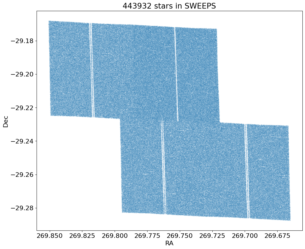
Sky Coverage

fig, ax = plt.subplots(figsize=(12, 10))
ax.scatter('RA', 'Dec', data=tab, s=1, alpha=0.1)
ax.set(xlabel='RA', ylabel='Dec', title=f'{len(tab)} stars in SWEEPS')
ax.invert_xaxis()

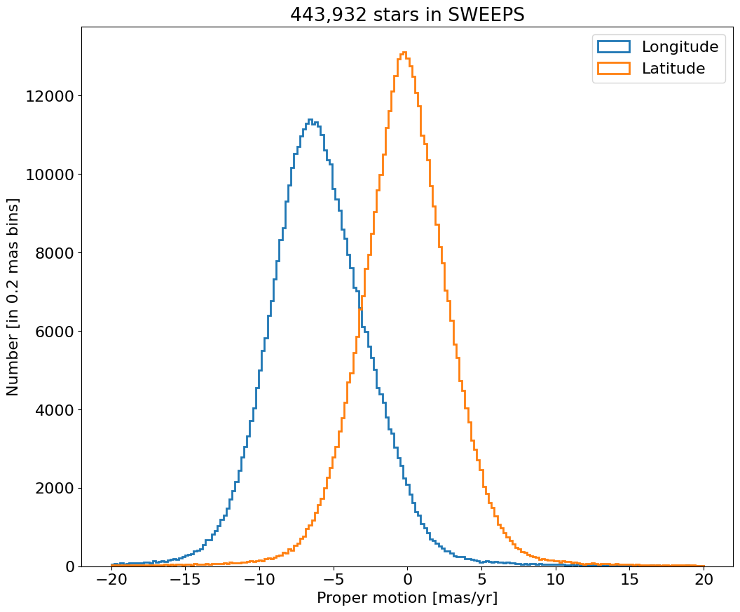
Proper Motion Histograms

Proper motion histograms for lon and lat

bin = 0.2
hrange = (-20, 20)
bincount = int((hrange[1]-hrange[0])/bin + 0.5) + 1

fig, ax = plt.subplots(figsize=(12, 10))
for col, label in zip(['lpm', 'bpm'], ['Longitude', 'Latitude']):
    ax.hist(col, data=tab, range=hrange, bins=bincount, label=label, histtype='step', linewidth=2)
ax.set(xlabel='Proper motion [mas/yr]', ylabel=f'Number [in {bin:.2} mas bins]', title=f'{len(tab):,} stars in SWEEPS')
_ = ax.legend()

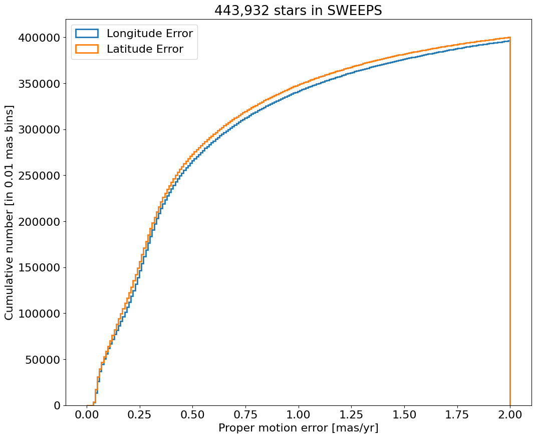
Proper motion error cumulative histogram for lon and lat

bin = 0.01
hrange = (0, 2)
bincount = int((hrange[1]-hrange[0])/bin + 0.5) + 1

fig, ax = plt.subplots(figsize=(12, 10))
for col, label in zip(['lpmerr', 'bpmerr'], ['Longitude Error', 'Latitude Error']):
    ax.hist(col, data=tab, range=hrange, bins=bincount, label=label, histtype='step', cumulative=1, linewidth=2)
ax.set(xlabel='Proper motion error [mas/yr]', ylabel=f'Cumulative number [in {bin:0.2} mas bins]', title=f'{len(tab):,} stars in SWEEPS')
_ = ax.legend(loc='upper left')

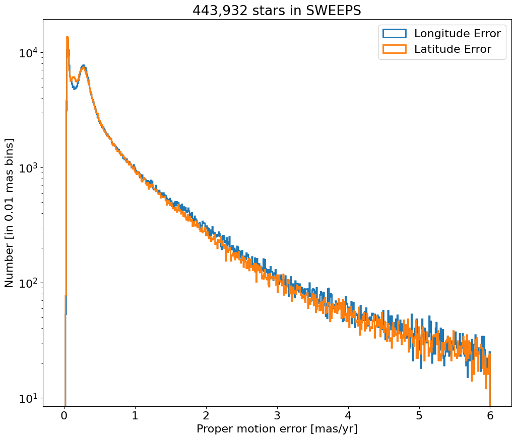
Proper motion error log histogram for lon and lat

bin = 0.01
hrange = (0, 6)
bincount = int((hrange[1]-hrange[0])/bin + 0.5) + 1

fig, ax = plt.subplots(figsize=(12, 10))
for col, label in zip(['lpmerr', 'bpmerr'], ['Longitude Error', 'Latitude Error']):
    ax.hist(col, data=tab, range=hrange, bins=bincount, label=label, histtype='step', linewidth=2)
ax.set(xlabel='Proper motion error [mas/yr]', ylabel=f'Number [in {bin:0.2} mas bins]', title=f'{len(tab):,} stars in SWEEPS', yscale='log')
_ = ax.legend(loc='upper right')

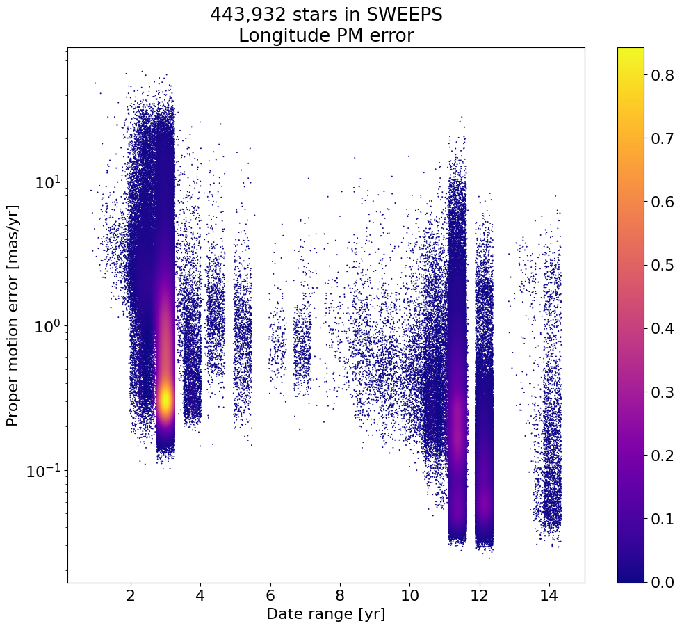
Proper motion error as a function of dT

Exclude objects with dT near zero, and to improve the plotting add a bit of random noise to spread out the quanitized time values.

# restrict to sources with dT > 1 year
dtmin = 1.0
w = np.where(tab['dT'] > dtmin)[0]
if ('rw' not in locals()) or len(rw) != len(w):
    rw = np.random.random(len(w))

x = np.array(tab['dT'][w]) + 0.5*(rw-0.5)
y = np.log(np.array(tab['lpmerr'][w]))

# Calculate the point density
t0 = time.time()
myPDF, axes = fastKDE.pdf(x.flatten(), y.flatten(), numPoints=2**9+1)
print("kde took {:.1f} sec".format(time.time()-t0))

# interpolate to get z values at points
finterp = RectBivariateSpline(axes[1], axes[0], myPDF)
z = finterp(y, x, grid=False)

# Sort the points by density, so that the densest points are plotted last
idx = z.argsort()
xs, ys, zs = x[idx], y[idx], z[idx]

# select a random subset of points in the most crowded regions to speed up plotting
wran = np.where(np.random.random(len(zs))*zs < 0.05)[0]
print("Plotting {} of {} points".format(len(wran), len(zs)))
xs = xs[wran]
ys = ys[wran]
zs = zs[wran]

kde took 1.6 sec

Plotting 177872 of 442682 points

fig, ax = plt.subplots(figsize=(12, 10))
sc = ax.scatter(xs, np.exp(ys), c=zs, s=2, edgecolors='none', cmap='plasma')
ax.set(xlabel='Date range [yr]', ylabel='Proper motion error [mas/yr]',
       title=f'{len(tab):,} stars in SWEEPS\nLongitude PM error', yscale='log')
_ = fig.colorbar(sc, ax=ax)

Proper motion error log histogram for lon and lat

Divide sample into points with \(<6\) years of data and points with more than 6 years of data.

bin = 0.01
hrange = (0, 6)
bincount = int((hrange[1]-hrange[0])/bin + 0.5) + 1

tsplit = 6
dmaglim = 0.05

wmag = np.where((tab['a_f606w_mad'] < dmaglim) & (tab['a_f814w_mad'] < dmaglim))[0]
w1 = wmag[tab['dT'][wmag] <= tsplit]
w2 = wmag[tab['dT'][wmag] > tsplit]

fig, (ax1, ax2) = plt.subplots(nrows=2, ncols=1, figsize=(12, 12), sharey=True, tight_layout=True)

for ax, w in zip([ax1, ax2], [w1, w2]):
    for col, label in zip(['lpmerr', 'bpmerr'], ['Longitude Error', 'Latitude Error']):
        data = tab[w]
        ax.hist(col, data=data, range=hrange, bins=bincount, label=label, histtype='step', linewidth=2)
        
ax1.set(xlabel='Proper motion error [mas/yr]', ylabel=f'Number [in {bin:0.2} mas bins]',
        title=f'{len(w1):,} stars in SWEEPS with dT < {tsplit} yrs, dmag < {dmaglim}', yscale='log')
ax2.set(xlabel='Proper motion error [mas/yr]', ylabel=f'Number [in {bin:0.2} mas bins]',
        title=f'{len(w2):,} stars in SWEEPS with dT > {tsplit} yrs, dmag < {dmaglim}', yscale='log')

ax1.legend()
ax2.legend()

<matplotlib.legend.Legend at 0x7f3fa96cb110>

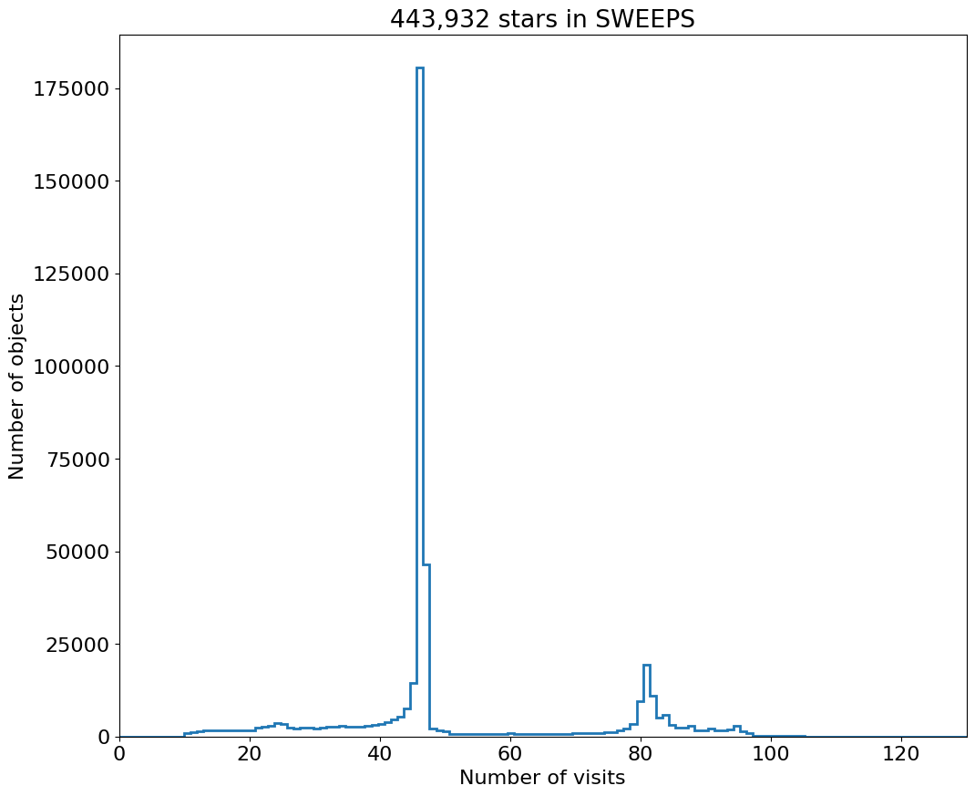
Number of Visits Histogram

bin = 1
hrange = (0, 130)
bincount = int((hrange[1]-hrange[0])/bin + 0.5) + 1

fig, ax = plt.subplots(figsize=(12, 10))
ax.hist('NumVisits', data=tab, range=hrange, bins=bincount, label='Number of visits ', histtype='step', linewidth=2)
ax.set(xlabel='Number of visits', ylabel='Number of objects', title=f'{len(tab):,} stars in SWEEPS')
_ = ax.margins(x=0)

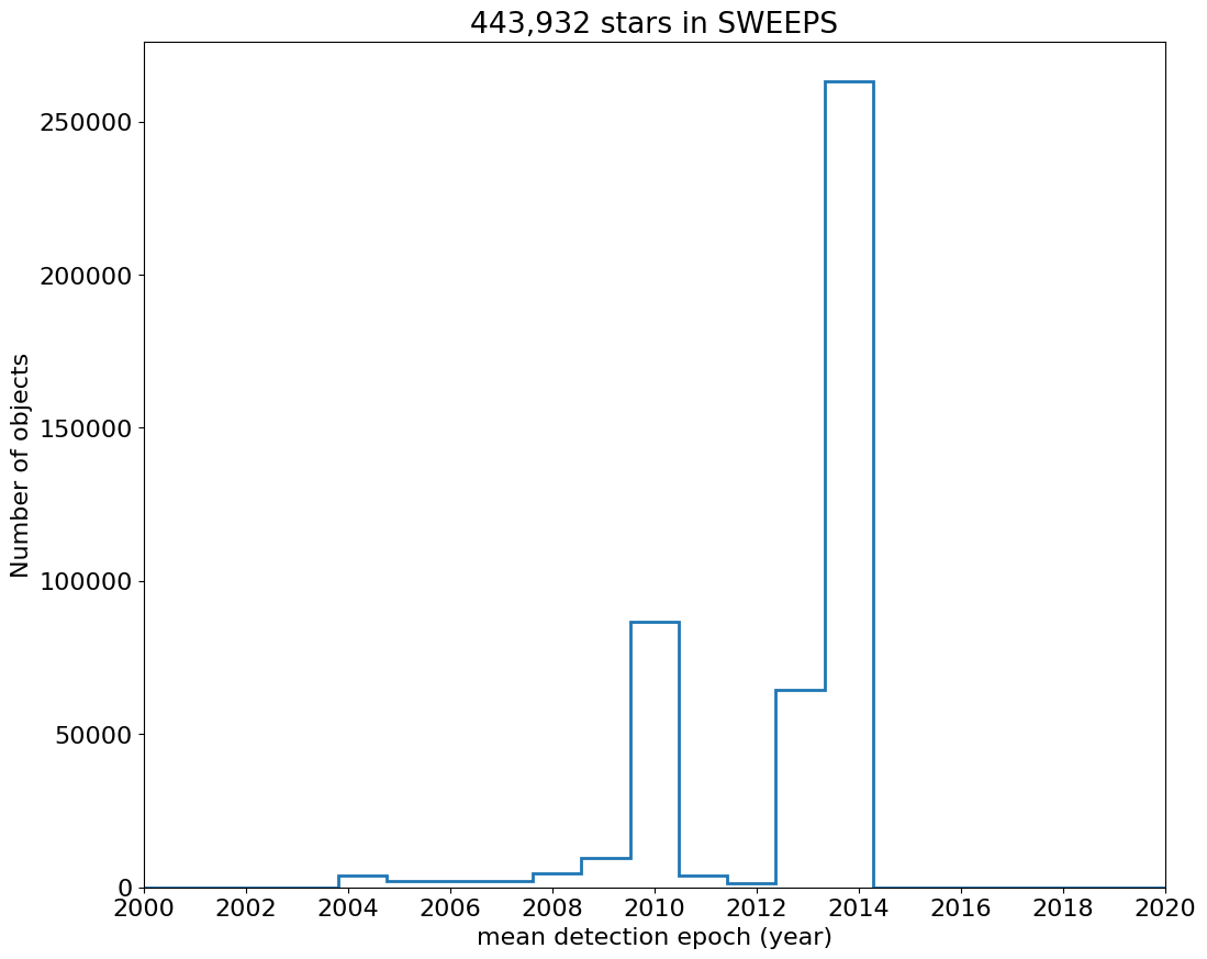
Time Histograms

First plot histogram of observation dates.

bin = 1
hrange = (2000, 2020)
bincount = int((hrange[1]-hrange[0])/bin + 0.5) + 1

fig, ax = plt.subplots(figsize=(12, 10))
ax.hist('yr', data=tab, range=hrange, bins=bincount, label='year ', histtype='step', linewidth=2)
ax.set(xlabel='mean detection epoch (year)', ylabel='Number of objects', title=f'{len(tab):,} stars in SWEEPS')
ax.set_xticks(ticks=range(2000, 2021, 2))
_ = ax.margins(x=0)

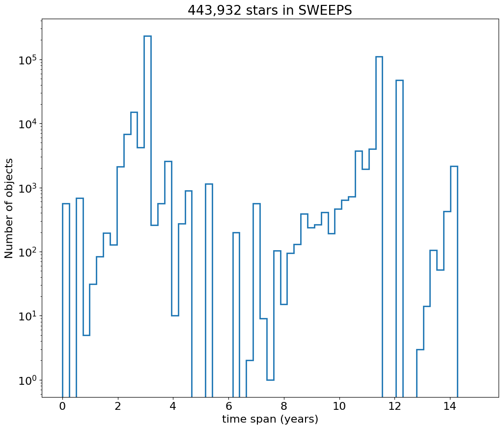
Then plot histogram of observation duration for the objects.

bin = 0.25
hrange = (0, 15)
bincount = int((hrange[1]-hrange[0])/bin + 0.5) + 1

fig, ax = plt.subplots(figsize=(12, 10))
ax.hist('dT', data=tab, range=hrange, bins=bincount, label='year ', histtype='step', linewidth=2)
_ = ax.set(xlabel='time span (years)', ylabel='Number of objects', title=f'{len(tab):,} stars in SWEEPS', yscale='log')

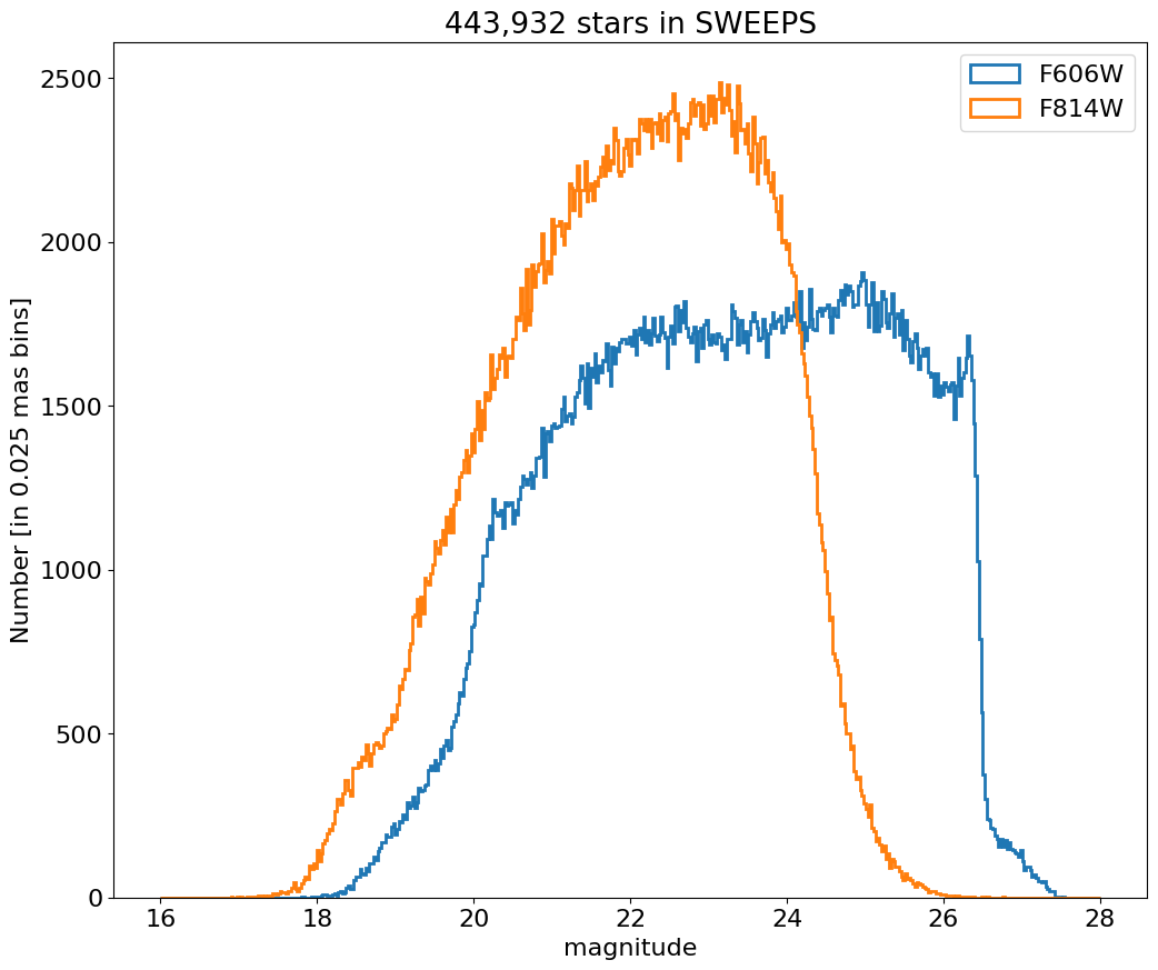
Magnitude Histograms

Aper2 magnitude histograms for F606W and F814W

bin = 0.025
hrange = (16, 28)
bincount = int((hrange[1]-hrange[0])/bin + 0.5) + 1

fig, ax = plt.subplots(figsize=(12, 10))
for col, label in zip(['a_f606w', 'a_f814w'], ['F606W', 'F814W']):
    ax.hist(col, data=tab, range=hrange, bins=bincount, label=label, histtype='step', linewidth=2)
ax.set(xlabel='magnitude', ylabel=f'Number [in {bin:0.2} mas bins]', title=f'{len(tab):,} stars in SWEEPS')
_ = ax.legend(loc='upper right')

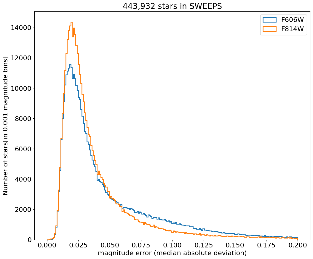
Aper2 magnitude error histograms for F606W and F814W

bin = 0.001
hrange = (0, 0.2)
bincount = int((hrange[1]-hrange[0])/bin + 0.5) + 1

fig, ax = plt.subplots(figsize=(12, 10))
for col, label in zip(['a_f606w_mad', 'a_f814w_mad'], ['F606W', 'F814W']):
    ax.hist(col, data=tab, range=hrange, bins=bincount, label=label, histtype='step', linewidth=2)
ax.set(xlabel='magnitude error (median absolute deviation)', ylabel=f'Number of stars[in {bin:0.2} magnitude bins]',
       title=f'{len(tab):,} stars in SWEEPS')
_ = ax.legend(loc='upper right')

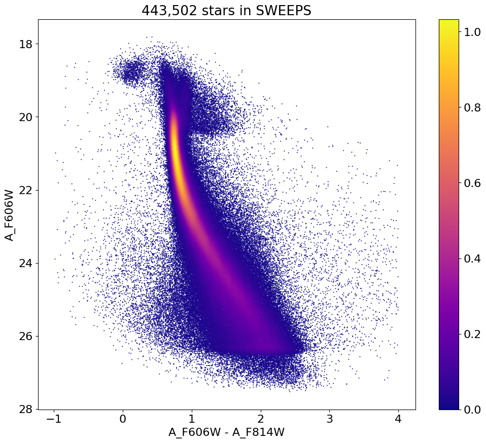
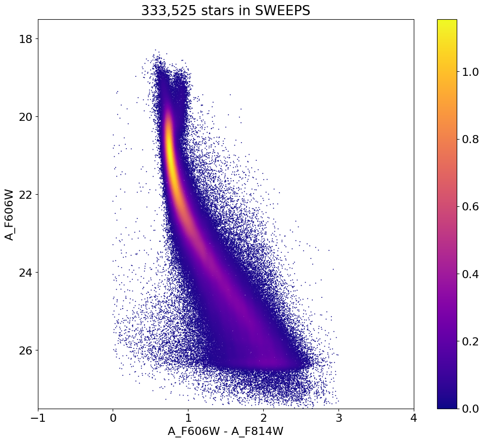
Color-Magnitude Diagram

Color-magnitude diagram

Plot the color-magnitude diagram for the ~440k points retrieved from the database. This uses fastkde to compute the kernel density estimate for the crowded plot, which is very fast. See https://pypi.org/project/fastkde/ for instructions – or just do
pip install fastkde

f606w = tab['a_f606w']
f814w = tab['a_f814w']
RminusI = f606w-f814w

# Calculate the point density
w = np.where((RminusI > -1) & (RminusI < 4))[0]
x = np.array(RminusI[w])
y = np.array(f606w[w])
t0 = time.time()
myPDF, axes = fastKDE.pdf(x, y, numPoints=2**10+1)
print("kde took {:.1f} sec".format(time.time()-t0))

# interpolate to get z values at points
finterp = RectBivariateSpline(axes[1], axes[0], myPDF)
z = finterp(y, x, grid=False)

# Sort the points by density, so that the densest points are plotted last
idx = z.argsort()
xs, ys, zs = x[idx], y[idx], z[idx]

# select a random subset of points in the most crowded regions to speed up plotting
wran = np.where(np.random.random(len(zs))*zs < 0.05)[0]
print(f"Plotting {len(wran)} of {len(zs)} points")
xs = xs[wran]
ys = ys[wran]
zs = zs[wran]

kde took 1.8 sec

Plotting 147935 of 443502 points

fig, ax = plt.subplots(figsize=(12, 10))
sc = ax.scatter(xs, ys, c=zs, s=2, edgecolors='none', cmap='plasma')
ax.set(xlabel='A_F606W - A_F814W', ylabel='A_F606W', title=f'{len(x):,} stars in SWEEPS')
ax.invert_yaxis()
fig.colorbar(sc, ax=ax)

<matplotlib.colorbar.Colorbar at 0x7f3fa4e43510>

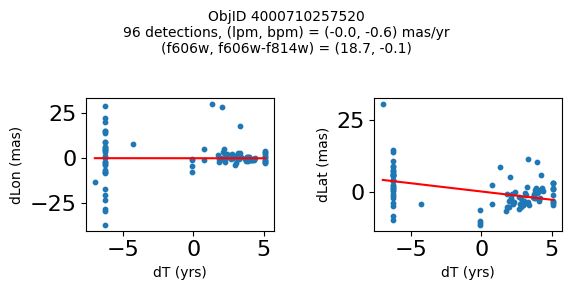
Detection Positions

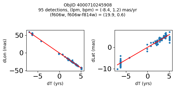
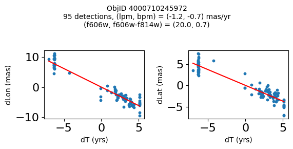
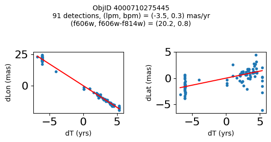
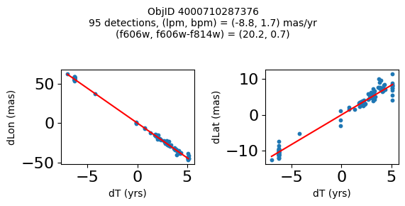
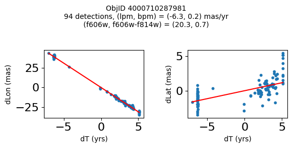
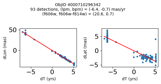
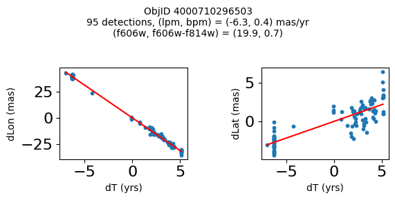
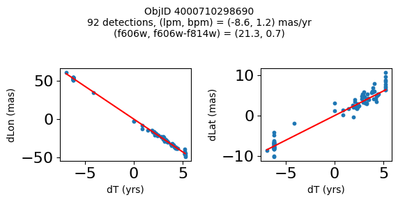
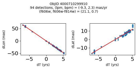
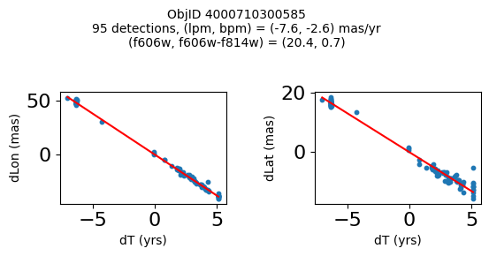
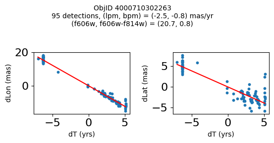
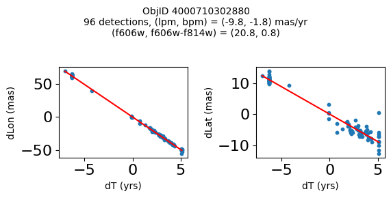
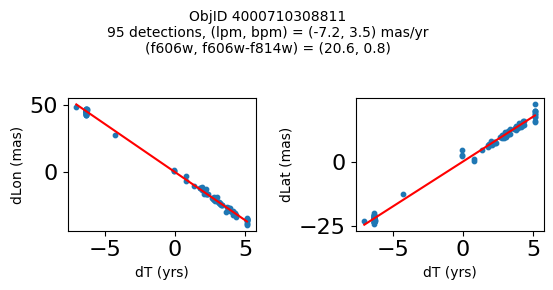
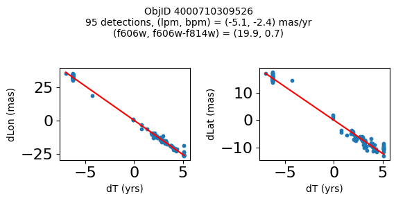
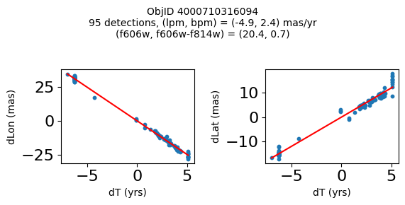
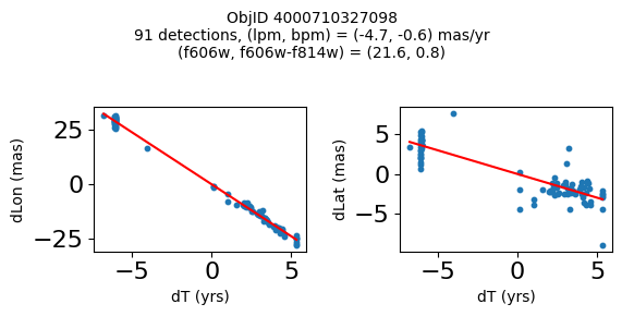
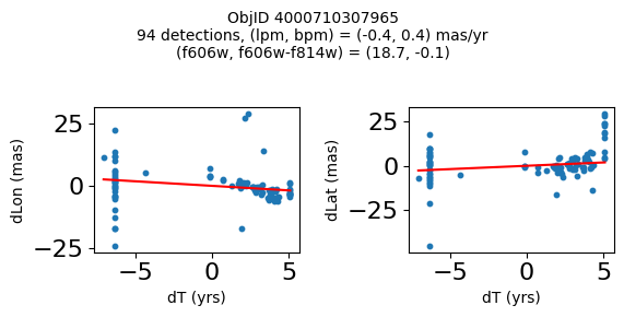
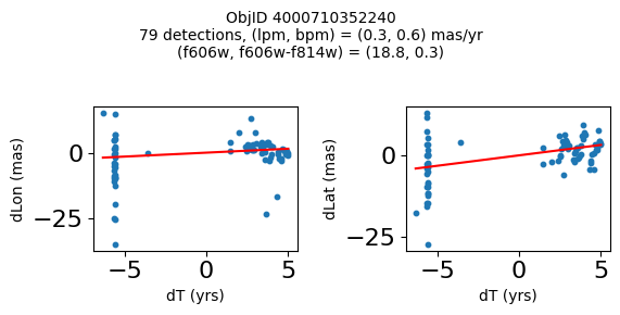
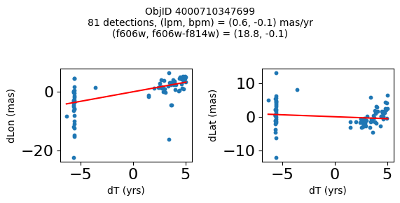
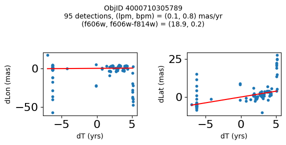
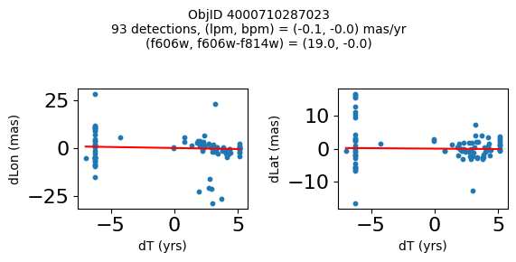
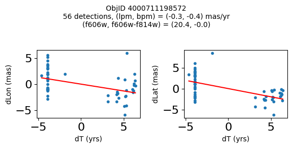
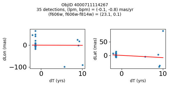
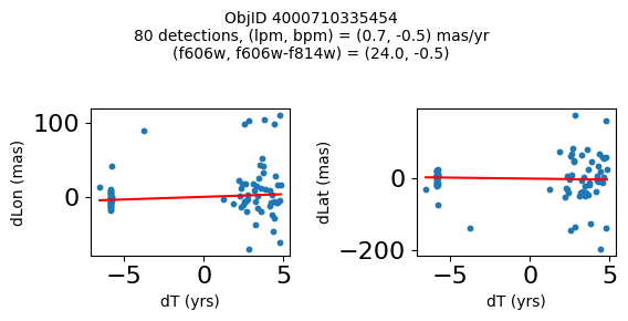
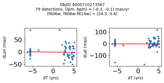
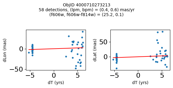
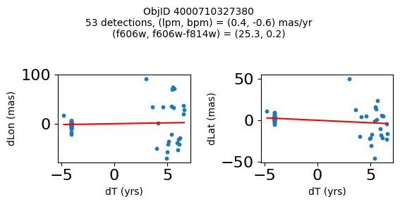
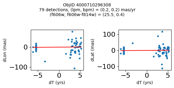
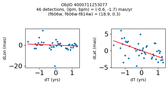
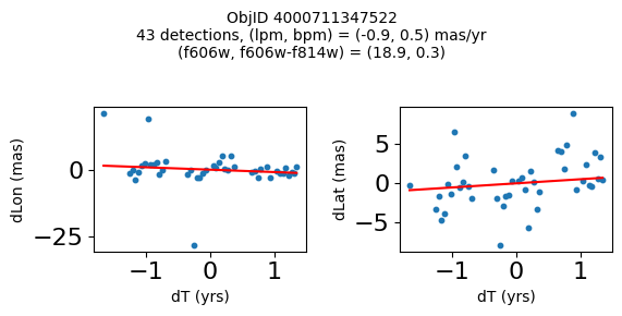
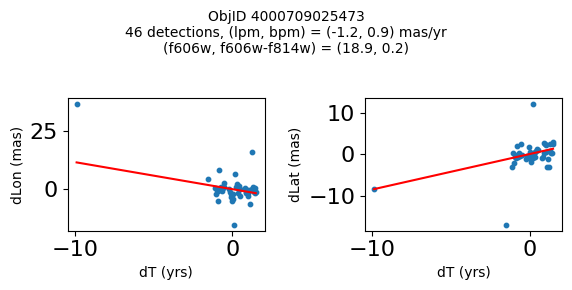
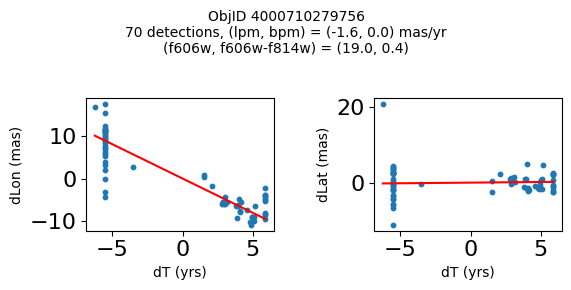
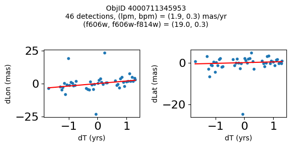
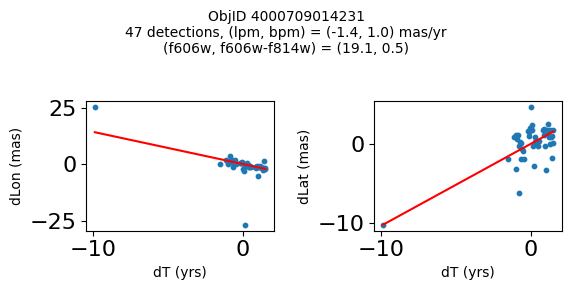
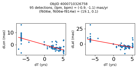
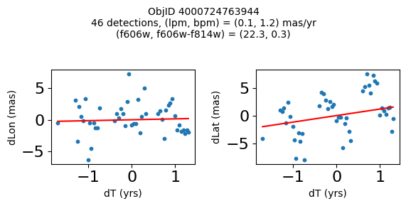
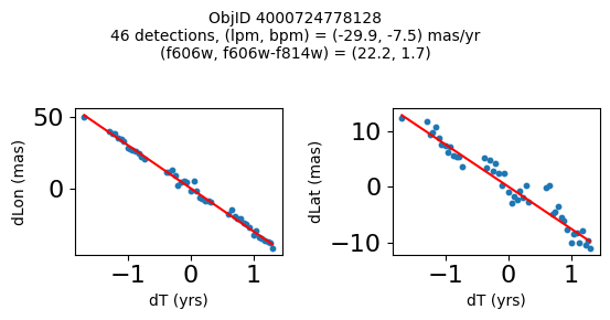
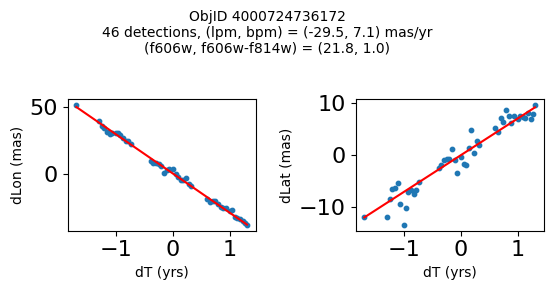
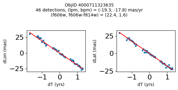
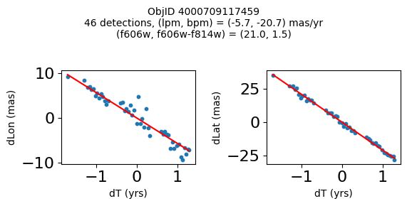
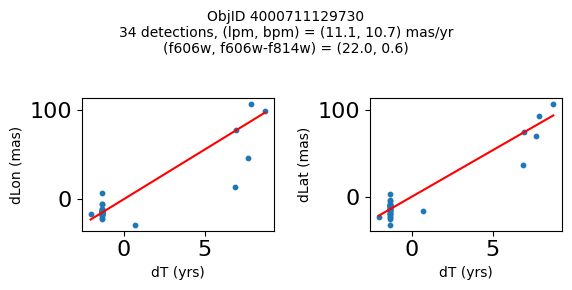
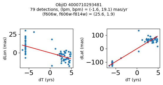
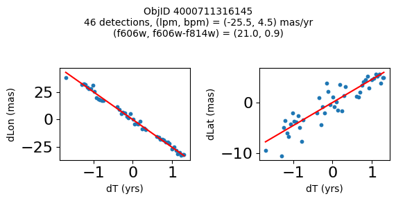
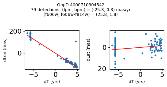
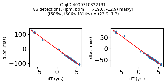
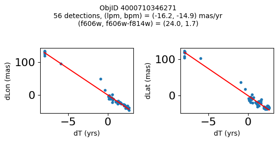
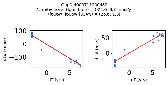
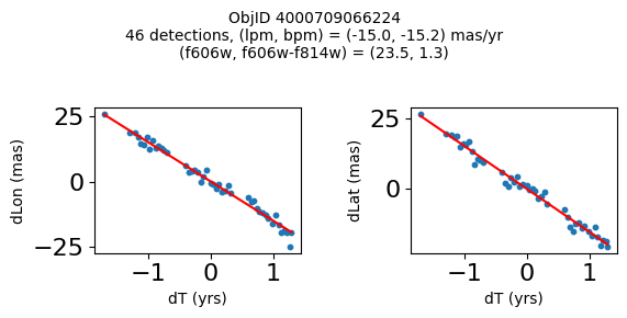
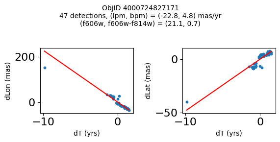
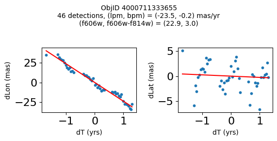
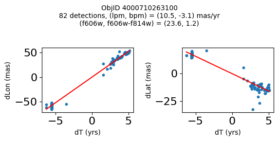
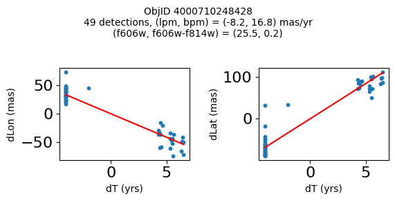
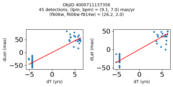
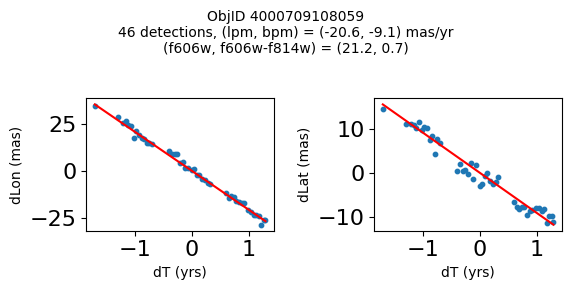
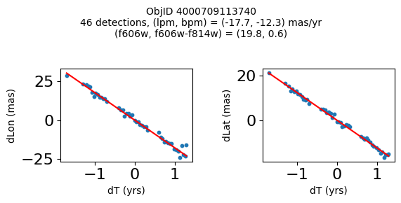
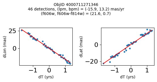
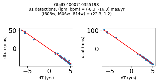
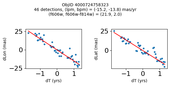
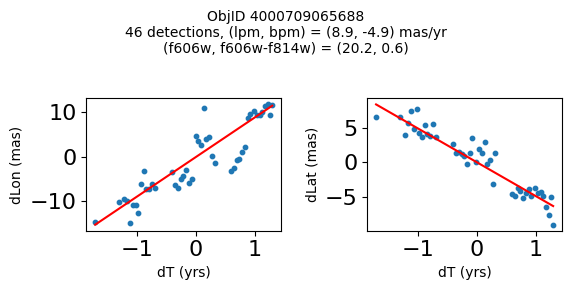
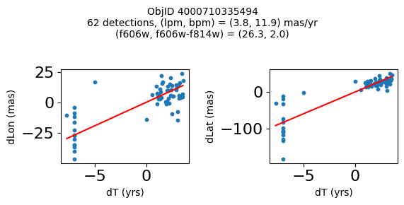
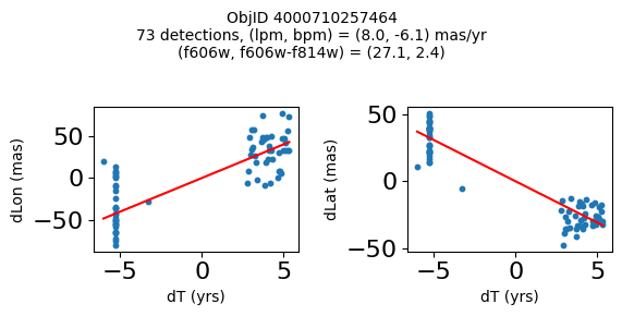
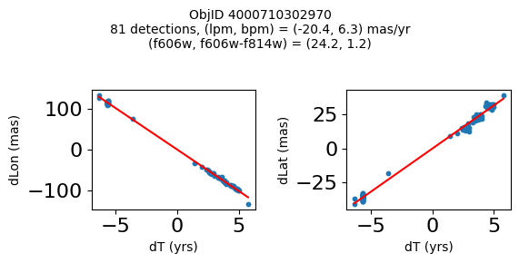
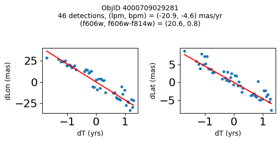
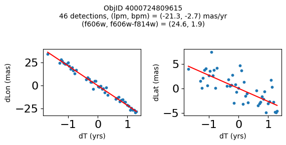
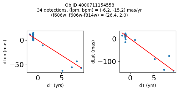
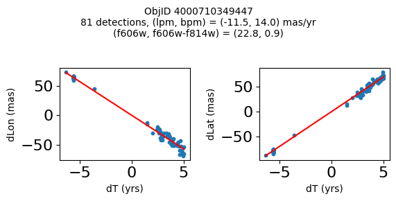
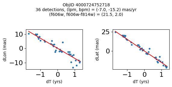
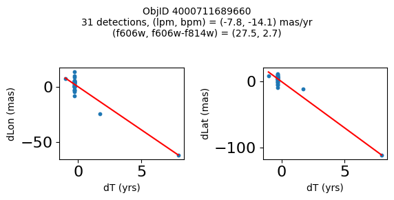
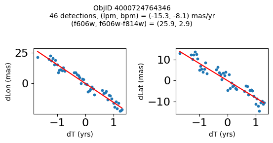
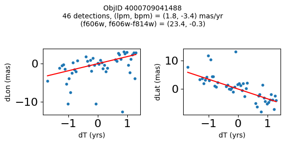
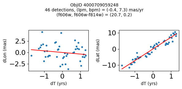
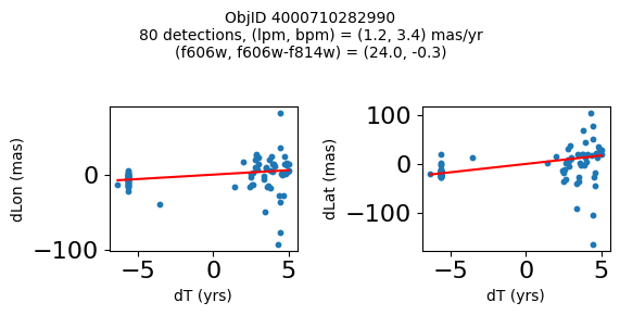
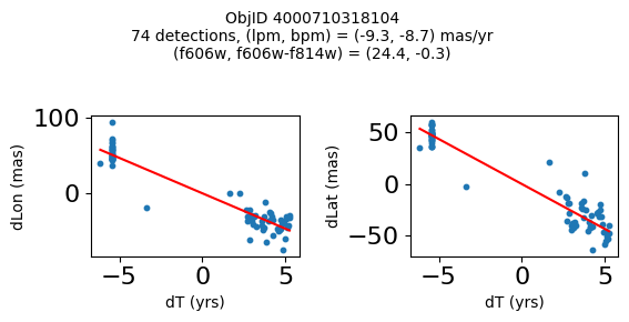
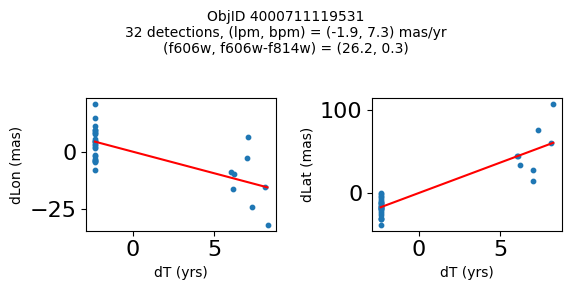
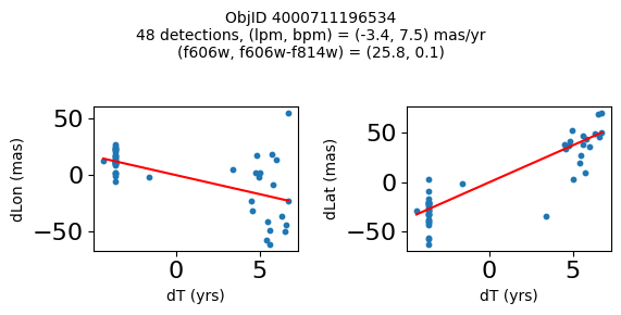
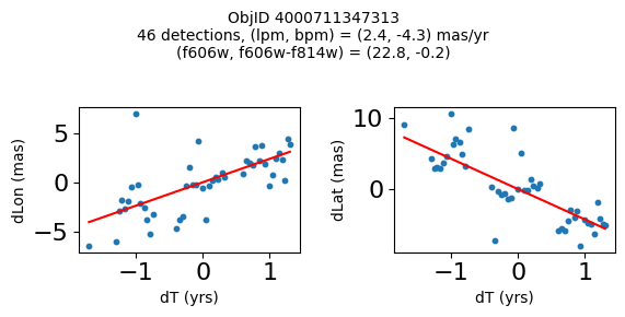
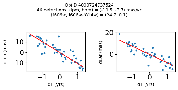
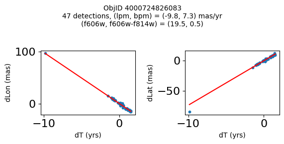
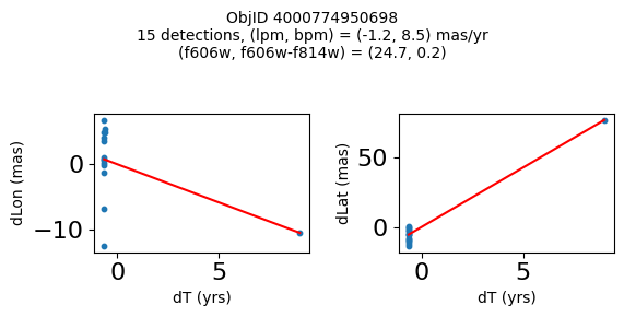
Define a function to plot the PM fit for an object.

# define function
def positions(Obj, jobs=None):
    """
    input parameter Obj is the value of the ObjID 
    optional jobs parameter re-uses casjobs jobs variable
    output plots change in (lon, lat) as a function of time
    overplots proper motion fit
    provides number of objects and magnitude/color information
    """
    if not jobs:
        jobs = mastcasjobs.MastCasJobs(context=HSCContext)

    # execute these as "system" queries so they don't fill up your Casjobs history

    # get the measured positions as a function of time
    query = f"""SELECT dT, dLon, dLat 
        from AstromSourcePositions where ObjID={Obj}
        order by dT
        """
    pos = jobs.quick(query, context=HSCContext, task_name="SWEEPS/Microlensing", astropy=True, system=True)
    
    # get the PM fit parameters
    query = f"""SELECT pmlon, pmlonerr, pmlat, pmlaterr
        from AstromProperMotions where ObjID={Obj}
        """
    pm = jobs.quick(query, context=HSCContext, task_name="SWEEPS/Microlensing", astropy=True, system=True)
    
    lpm = pm['pmlon'][0]
    bpm = pm['pmlat'][0]
    
    # get the intercept for the proper motion fit referenced to the start time
    # time between mean epoch and zero (ref) epoch (years)

    # get median magnitudes and colors for labeling
    query = f"""SELECT a_f606w=i1.MagMed, a_f606_m_f814w=i1.MagMed-i2.MagMed
        from AstromSumMagAper2 i1 
        join AstromSumMagAper2 i2 on i1.ObjID=i2.ObjID 
        where i1.ObjID={Obj} and i1.filter='f606w' and i2.filter='f814w' 
        """
    phot = jobs.quick(query, context=HSCContext, task_name="SWEEPS/Microlensing", astropy=True, system=True)
    f606w = phot['a_f606w'][0]
    f606wmf814w = phot['a_f606_m_f814w'][0]

    x = pos['dT']
    # xpm = np.linspace(0, max(x), 10)
    xpm = np.array([x.min(), x.max()])
        
    y1 = pos['dLon']
    ypm1 = lpm*xpm
    
    y2 = pos['dLat']
    ypm2 = bpm*xpm

    # plot figure
    fig, (ax1, ax2) = plt.subplots(nrows=1, ncols=2, figsize=(6, 3), tight_layout=True)
    
    ax1.scatter(x, y1, s=10)
    ax1.plot(xpm, ypm1, '-r')
    
    ax2.scatter(x, y2, s=10)
    ax2.plot(xpm, ypm2, '-r')
    
    ax1.set_xlabel('dT (yrs)', fontsize=10)
    ax1.set_ylabel('dLon (mas)', fontsize=10)
    ax2.set_xlabel('dT (yrs)', fontsize=10)
    ax2.set_ylabel('dLat (mas)', fontsize=10)
    
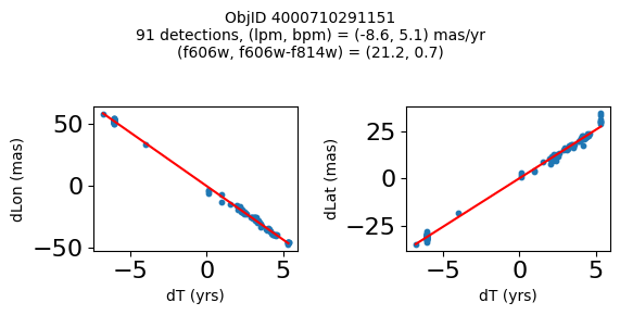
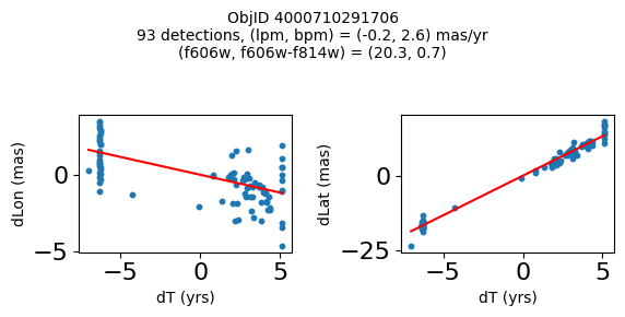
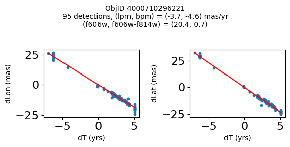
    fig.suptitle(f"ObjID {Obj}"
                 f"\n{len(x)} detections, (lpm, bpm) = ({lpm:.1f}, {bpm:.1f}) mas/yr"
                 f"\n(f606w, f606w-f814w) = ({f606w:.1f}, {f606wmf814w:.1f})", size=10)
    
    plt.show()
    plt.close()

Plot positions of objects that are detected in more than 90 visits with a median absolute deviation from the fit of less than 1.5 mas and proper motion error less than 1.0 mas/yr.

n = tab['NumVisits']
dev = tab['pmdev']
objid = tab['ObjID']
lpmerr0 = np.array(tab['lpmerr'])
bpmerr0 = np.array(tab['bpmerr'])
wi = np.where((dev < 1.5) & (n > 90) & (np.sqrt(bpmerr0**2+lpmerr0**2) < 1.0))[0]
print(f"Plotting {len(wi)} objects")
for o in objid[wi]:
    positions(o, jobs=jobs)

Plotting 21 objects

Good Photometric Objects

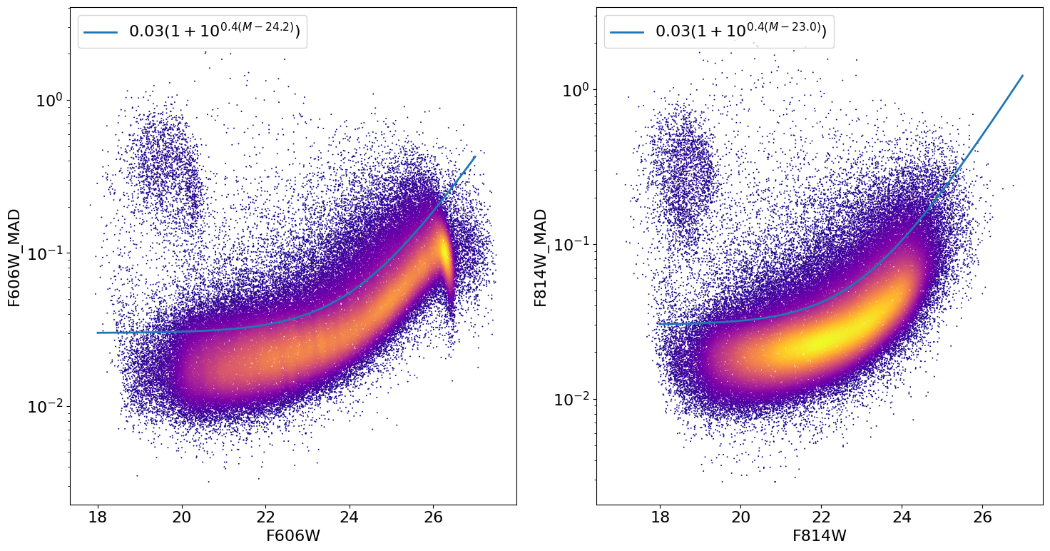
Look at photometric error distribution to pick out good photometry objects as a function of magnitude

The photometric error is mainly a function of magnitude. We make a cut slightly above the typical error to exclude objects that have poor photometry. (In the SWEEPS field, that most often is the result of blending and crowding.)

f606w = tab['a_f606w']
f814w = tab['a_f814w']
RminusI = f606w-f814w

w = np.where((RminusI > -1) & (RminusI < 4))[0]
f606w_mad = tab['a_f606w_mad']
f814w_mad = tab['a_f814w_mad']

t0 = time.time()
# Calculate the point density
x1 = np.array(f606w[w])
y1 = np.array(f606w_mad[w])
y1log = np.log(y1)
myPDF1, axes1 = fastKDE.pdf(x1, y1log, numPoints=2**10+1)
finterp = RectBivariateSpline(axes1[1], axes1[0], myPDF1)
z1 = finterp(y1log, x1, grid=False)
# Sort the points by density, so that the densest points are plotted last
idx = z1.argsort()
xs1, ys1, zs1 = x1[idx], y1[idx], z1[idx]

# select a random subset of points in the most crowded regions to speed up plotting
wran = np.where(np.random.random(len(zs1))*zs1 < 0.05)[0]
print(f"Plotting {len(wran)} of {len(zs1)} points")
xs1 = xs1[wran]
ys1 = ys1[wran]
zs1 = zs1[wran]

x2 = np.array(f814w[w])
y2 = np.array(f814w_mad[w])
y2log = np.log(y2)
myPDF2, axes2 = fastKDE.pdf(x2, y2log, numPoints=2**10+1)
finterp = RectBivariateSpline(axes2[1], axes2[0], myPDF2)
z2 = finterp(y2log, x2, grid=False)
idx = z2.argsort()
xs2, ys2, zs2 = x2[idx], y2[idx], z2[idx]
print(f"{(time.time()-t0):.1f} s: completed kde")

# select a random subset of points in the most crowded regions to speed up plotting
wran = np.where(np.random.random(len(zs2))*zs2 < 0.05)[0]
print(f"Plotting {len(wran)} of {len(zs2)} points")
xs2 = xs2[wran]
ys2 = ys2[wran]
zs2 = zs2[wran]

xr = (18, 27)
xx = np.arange(501)*(xr[1]-xr[0])/500.0 + xr[0]
xcut1 = 24.2
xnorm1 = 0.03
xcut2 = 23.0
xnorm2 = 0.03

# only plot a subset of the points to speed things up
qsel = 3
xs1 = xs1[::qsel]
ys1 = ys1[::qsel]
zs1 = zs1[::qsel]
xs2 = xs2[::qsel]
ys2 = ys2[::qsel]
zs2 = zs2[::qsel]

Plotting 274435 of 443502 points

4.4 s: completed kde
Plotting 250645 of 443502 points

fig, (ax1, ax2) = plt.subplots(nrows=1, ncols=2, figsize=(15, 8), tight_layout=True)

ax1.scatter(xs1, ys1, c=zs1, s=2, edgecolors='none', cmap='plasma')
ax1.plot(xx, xnorm1 * (1. + 10.**(0.4*(xx-xcut1))), linewidth=2.0,
         label=f'${xnorm1:.2f} (1+10^{{0.4(M-{xcut1:.1f})}})$')

ax2.scatter(xs2, ys2, c=zs2, s=2, edgecolors='none', cmap='plasma')
ax2.plot(xx, xnorm2 * (1. + 10.**(0.4*(xx-xcut2))), linewidth=2.0,
         label=f'${xnorm2:.2f} (1+10^{{0.4(M-{xcut2:.1f})}})$')

ax1.legend(loc='upper left')
ax2.legend(loc='upper left')

ax1.set(xlabel='F606W', ylabel='F606W_MAD', yscale='log')
ax2.set(xlabel='F814W', ylabel='F814W_MAD', yscale='log')

[Text(0.5, 0, 'F814W'), Text(0, 0.5, 'F814W_MAD'), None]

Define function to apply noise cut and plot color-magnitude diagram with cut

Note that we reduce the R-I range to 0-3 here because there are very few objects left bluer than R-I = 0 or redder than R-I = 3.

def noisecut(tab, factor=1.0):
    """Return boolean array with noise cut in f606w and f814w using model
    factor is normalization factor to use (>1 means allow more noise)
    """
    f606w = tab['a_f606w']
    f814w = tab['a_f814w']
    f606w_mad = tab['a_f606w_mad']
    f814w_mad = tab['a_f814w_mad']
    
    # noise model computed above
    xcut_f606w = 24.2
    xnorm_f606w = 0.03 * factor
    xcut_f814w = 23.0
    xnorm_f814w = 0.03 * factor
    return ((f606w_mad < xnorm_f606w*(1+10.0**(0.4*(f606w-xcut_f606w))))
            & (f814w_mad < xnorm_f814w*(1+10.0**(0.4*(f814w-xcut_f814w)))))

# low-noise objects
good = noisecut(tab, factor=1.0)

# Calculate the point density
w = np.where((RminusI > 0) & (RminusI < 3) & good)[0]
x = np.array(RminusI[w])
y = np.array(f606w[w])
t0 = time.time()
myPDF, axes = fastKDE.pdf(x, y, numPoints=2**10+1)
print(f"kde took {(time.time()-t0):.1f} sec")

# interpolate to get z values at points
finterp = RectBivariateSpline(axes[1], axes[0], myPDF)
z = finterp(y, x, grid=False)

# Sort the points by density, so that the densest points are plotted last
idx = z.argsort()
xs, ys, zs = x[idx], y[idx], z[idx]

# select a random subset of points in the most crowded regions to speed up plotting
wran = np.where(np.random.random(len(zs))*zs < 0.075)[0]
print(f"Plotting {len(wran)} of {len(zs)} points")
xs = xs[wran]
ys = ys[wran]
zs = zs[wran]

kde took 1.5 sec

Plotting 129618 of 333525 points

fig, ax = plt.subplots(figsize=(12, 10))

sc = ax.scatter(xs, ys, c=zs, s=2, edgecolors='none', cmap='plasma')
ax.set(xlabel='A_F606W - A_F814W', ylabel='A_F606W',
       title=f'{len(x):,} stars in SWEEPS', xlim=(-1, 4), ylim=(27.5, 17.5))
_ = fig.colorbar(sc, ax=ax)

Science Applications

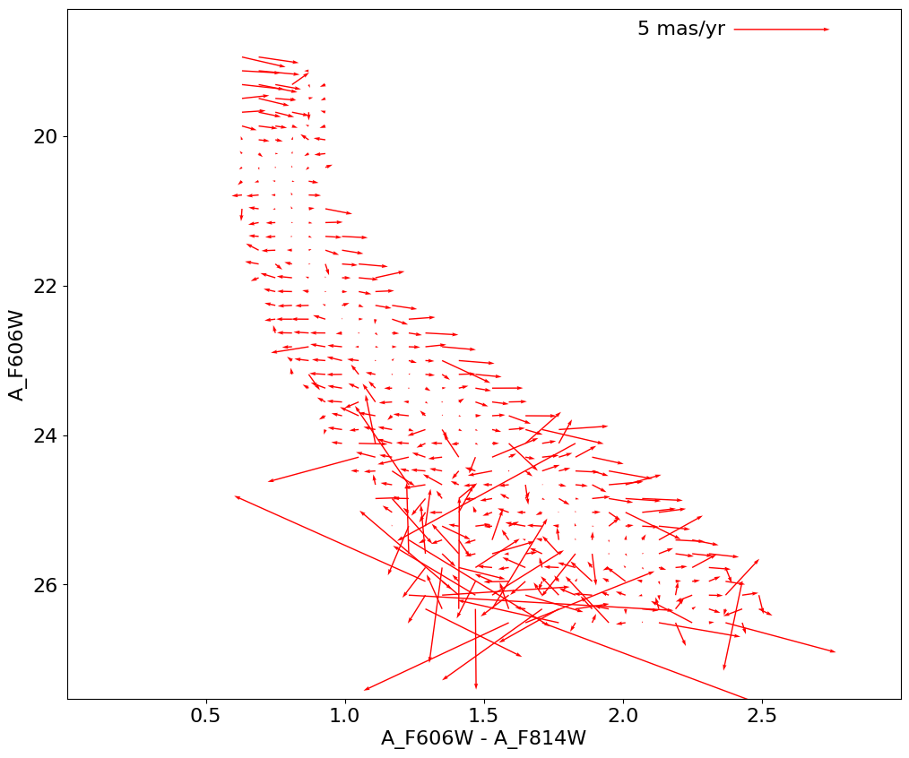
Proper Motions of Good Objects

Average proper motion in color-magnitude bins

# good defined above
f606w = tab['a_f606w']
f814w = tab['a_f814w']
RminusI = f606w-f814w
w = np.where((RminusI > 0) & (RminusI < 3) & good)[0]
lpm = np.array(tab['lpm'][w])
bpm = np.array(tab['bpm'][w])
x = np.array(RminusI[w])
y = np.array(f606w[w])

nbins = 50
count2d, yedge, xedge = np.histogram2d(y, x, bins=nbins)
lpm_sum = np.histogram2d(y, x, bins=nbins, weights=lpm-lpm.mean())[0]
bpm_sum = np.histogram2d(y, x, bins=nbins, weights=bpm-bpm.mean())[0]
lpm_sumsq = np.histogram2d(y, x, bins=nbins, weights=(lpm-lpm.mean())**2)[0]
bpm_sumsq = np.histogram2d(y, x, bins=nbins, weights=(bpm-bpm.mean())**2)[0]

ccount = count2d.clip(1) 
lpm_mean = lpm_sum/ccount
bpm_mean = bpm_sum/ccount
lpm_rms = np.sqrt(lpm_sumsq/ccount-lpm_mean**2)
bpm_rms = np.sqrt(bpm_sumsq/ccount-bpm_mean**2)
lpm_msigma = lpm_rms/np.sqrt(ccount)
bpm_msigma = bpm_rms/np.sqrt(ccount)

ww = np.where(count2d > 100)
yy, xx = np.mgrid[:nbins, :nbins]
xx = (0.5*(xedge[1:]+xedge[:-1]))[xx]
yy = (0.5*(yedge[1:]+yedge[:-1]))[yy]

fig, ax = plt.subplots(figsize=(12, 10))

Q = ax.quiver(xx[ww], yy[ww], lpm_mean[ww], bpm_mean[ww], color='red', width=0.0015)
qlength = 5
ax.quiverkey(Q, 0.8, 0.97, qlength, f'{qlength} mas/yr', coordinates='axes', labelpos='W')
ax.invert_yaxis()
_ = ax.set(xlabel='A_F606W - A_F814W', ylabel='A_F606W',
           xlim=(xedge[0], xedge[-1]), ylim=(yedge[-1], yedge[0]))

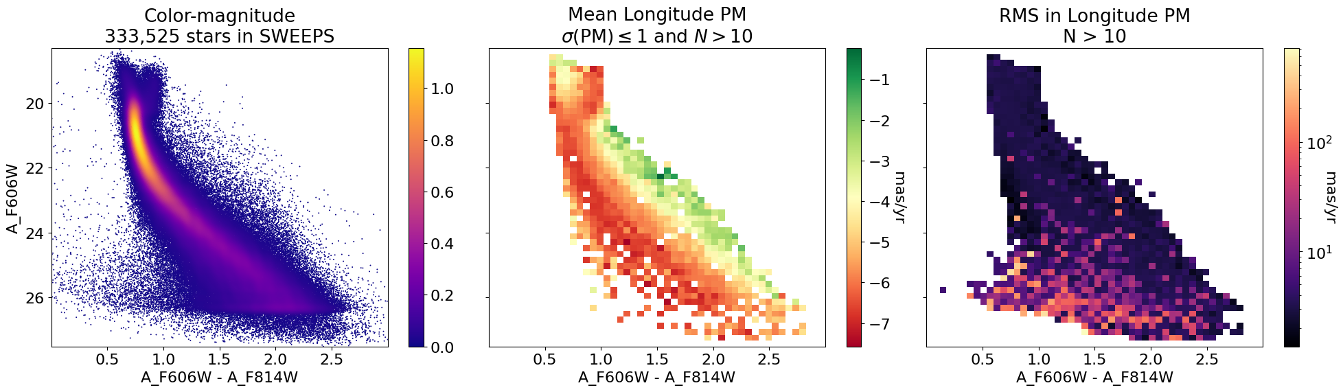
RMS in longitude PM as a function of color/magnitude

Mean longitude PM as image

fig, (ax1, ax2, ax3) = plt.subplots(nrows=1, ncols=3, figsize=(20, 6), tight_layout=True, sharey=True)

# plot ax1
p1 = ax1.scatter(xs, ys, c=zs, s=2, edgecolors='none', cmap='plasma')
ax1.set(xlabel='A_F606W - A_F814W', ylabel='A_F606W',
        title=f'Color-magnitude\n{len(x):,} stars in SWEEPS')
ax1.set(xlim=(xedge[0], xedge[-1]), ylim=(yedge[0], yedge[-1]))
ax1.invert_yaxis()
fig.colorbar(p1, ax=ax1)

# plot ax2
mask = (lpm_msigma <= 1.0) & (count2d > 10)
im2 = (lpm_mean+lpm.mean())*mask
im2[~mask] = np.nan
vmax = np.nanmax(np.abs(im2))

p2 = ax2.imshow(im2, cmap='RdYlGn', aspect="auto", origin="lower",
                extent=(xedge[0], xedge[-1], yedge[0], yedge[-1]))
ax2.set(xlabel='A_F606W - A_F814W',
        title='Mean Longitude PM\n$\\sigma(\\mathrm{PM}) \\leq 1$ and $N > 10$')
ax2.set(xlim=(xedge[0], xedge[-1]), ylim=(yedge[0], yedge[-1]))
ax2.invert_yaxis()
cb2 = fig.colorbar(p2, ax=ax2)
cb2.ax.set_ylabel('mas/yr', rotation=270, labelpad=15)

# plat ax3
im3 = lpm_rms*(count2d > 10)

p3 = ax3.imshow(im3, cmap='magma', aspect="auto", origin="lower",
                extent=(xedge[0], xedge[-1], yedge[0], yedge[-1]),
                norm=LogNorm(vmin=im3[im3 > 0].min(), vmax=im3.max()))
ax3.set(xlabel='A_F606W - A_F814W',
        title='RMS in Longitude PM\nN > 10')
ax3.set(xlim=(xedge[0], xedge[-1]), ylim=(yedge[0], yedge[-1]))
ax3.invert_yaxis()
cb3 = fig.colorbar(p3, ax=ax3)
_ = cb3.ax.set_ylabel('mas/yr', rotation=270)

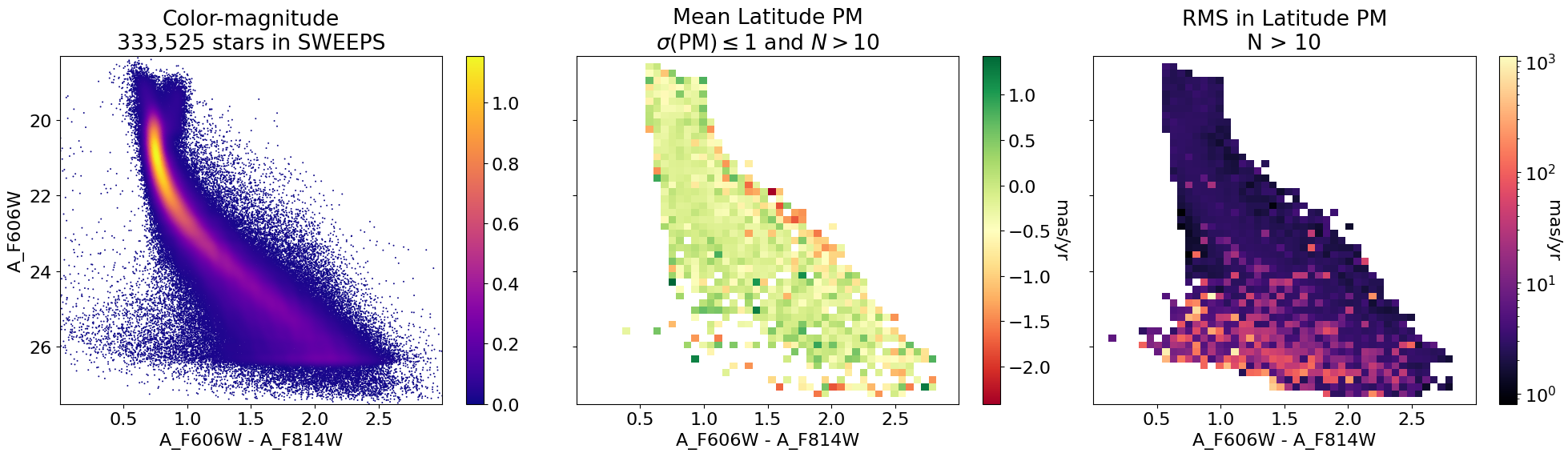
Mean latitude PM as image

fig, (ax1, ax2, ax3) = plt.subplots(nrows=1, ncols=3, figsize=(20, 6), tight_layout=True, sharey=True)

# plot ax1
p1 = ax1.scatter(xs, ys, c=zs, s=2, edgecolors='none', cmap='plasma')
ax1.set(xlabel='A_F606W - A_F814W', ylabel='A_F606W',
        title=f'Color-magnitude\n{len(x):,} stars in SWEEPS')
ax1.set(xlim=(xedge[0], xedge[-1]), ylim=(yedge[0], yedge[-1]))
ax1.invert_yaxis()
fig.colorbar(p1, ax=ax1)

# plot ax2
mask = (bpm_msigma <= 1.0) & (count2d > 10)
im2 = (bpm_mean+bpm.mean())*mask
im2[~mask] = np.nan
vmax = np.nanmax(np.abs(im2))

p2 = ax2.imshow(im2, cmap='RdYlGn', aspect="auto", origin="lower",
                extent=(xedge[0], xedge[-1], yedge[0], yedge[-1]))
ax2.set(xlabel='A_F606W - A_F814W',
        title='Mean Latitude PM\n$\\sigma(\\mathrm{PM}) \\leq 1$ and $N > 10$')
ax2.set(xlim=(xedge[0], xedge[-1]), ylim=(yedge[0], yedge[-1]))
ax2.invert_yaxis()
cb2 = fig.colorbar(p2, ax=ax2)
cb2.ax.set_ylabel('mas/yr', rotation=270, labelpad=15)

# plot ax3
im3 = bpm_rms*(count2d > 10)

p3 = ax3.imshow(im3, cmap='magma', aspect="auto", origin="lower",
                extent=(xedge[0], xedge[-1], yedge[0], yedge[-1]),
                norm=LogNorm(vmin=im3[im3 > 0].min(), vmax=im3.max()))
ax3.set(xlabel='A_F606W - A_F814W',
        title='RMS in Latitude PM\nN > 10')
ax3.set(xlim=(xedge[0], xedge[-1]), ylim=(yedge[0], yedge[-1]))
ax3.invert_yaxis()
cb3 = fig.colorbar(p3, ax=ax3)
_ = cb3.ax.set_ylabel('mas/yr', rotation=270)

Proper Motions in Bulge and Disk

Fit a smooth function to the main ridgeline of color-magnitude diagram

Fit the R-I vs R values, but force the function to increase montonically with R. We use a log transform of the y coordinate to help.

# locate ridge line
iridgex = np.argmax(myPDF, axis=1)
pdfx = myPDF[np.arange(len(iridgex), dtype=int), iridgex]
# pdfx = myPDF.max(axis=1)
wx = np.where(pdfx > 0.1)[0]
iridgex = iridgex[wx]
# use weighted sum of 2*hw+1 points around peak
hw = 10
pridgex = 0.0
pdenom = 0.0
for k in range(-hw, hw+1):
    wt = myPDF[wx, iridgex+k]
    pridgex = pridgex + k*wt
    pdenom = pdenom + wt
pridgex = iridgex + pridgex/pdenom
ridgex = np.interp(pridgex, np.arange(len(axes[0])), axes[0])

# Fit the data using a polynomial model
x0 = axes[1][wx].min()
x1 = axes[1][wx].max()
p_init = models.Polynomial1D(9)
fit_p = fitting.LinearLSQFitter()
xx = (axes[1][wx]-x0)/(x1-x0)
yoff = 0.65
yy = np.log(ridgex - yoff)
p = fit_p(p_init, xx, yy)

# define useful functions for the ridge line


def ridge_color(f606w, function=p, yoff=yoff, x0=x0, x1=x1):
    """Return R-I position of ridge line as a function of f606w magnitude
    
    function, yoff, x0, x1 are from polynomial fit above
    """
    return yoff + np.exp(p((f606w-x0)/(x1-x0)))


# calculate grid of function values for approximate inversion
rxgrid = axes[1][wx]
rygrid = ridge_color(rxgrid)
color_domain = [rygrid[0], rygrid[-1]]
mag_domain = [axes[1][wx[0]], axes[1][wx[-1]]]
print(f"color_domain {color_domain}")
print(f"mag_domain   {mag_domain}")


def ridge_mag(RminusI, xgrid=rxgrid, ygrid=rygrid):
    """Return f606w position of ridge line as a function of R-I color
    
    Uses simple linear interpolation to get approximate value
    """
    f606w = np.interp(RminusI, ygrid, xgrid)
    f606w[(RminusI < ygrid[0]) | (RminusI > ygrid[-1])] = np.nan
    return f606w

color_domain [0.6883374859498668, 2.156051675824816]
mag_domain   [19.356585323810577, 26.480549454689026]

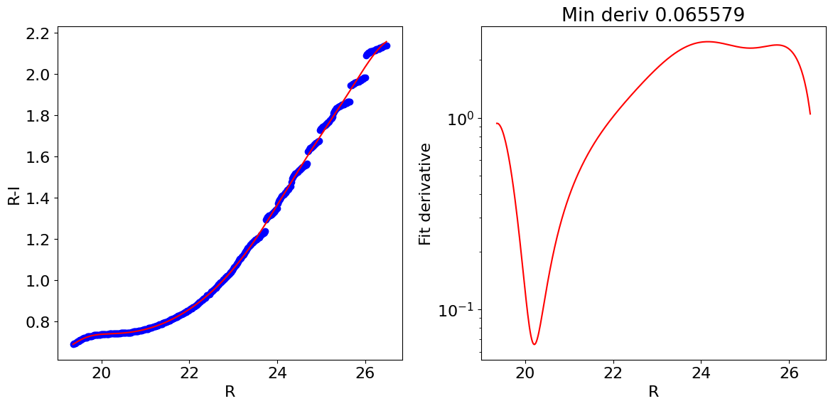
Plot the results to check that they look reasonable.

ridgexf = yoff + np.exp(p(xx))

fig, (ax1, ax2) = plt.subplots(nrows=1, ncols=2, figsize=(12, 6), tight_layout=True)

ax1.plot(axes[1][wx], ridgex, 'bo')
ax1.plot(axes[1][wx], ridgexf, color='red')
ax1.set(xlabel='R', ylabel='R-I')

# check the derivative plot to see if it stays positive
deriv = (np.exp(p(xx)) * 
         models.Polynomial1D.horner(xx, (p.parameters * np.arange(len(p.parameters)))[1:]))

ax2.semilogy(axes[1][wx], np.exp(p(xx)) *
             models.Polynomial1D.horner(xx, (p.parameters * np.arange(len(p.parameters)))[1:]), color='red')
_ = ax2.set(xlabel='R', ylabel='Fit derivative', title=f'Min deriv {deriv.min():.6f}')

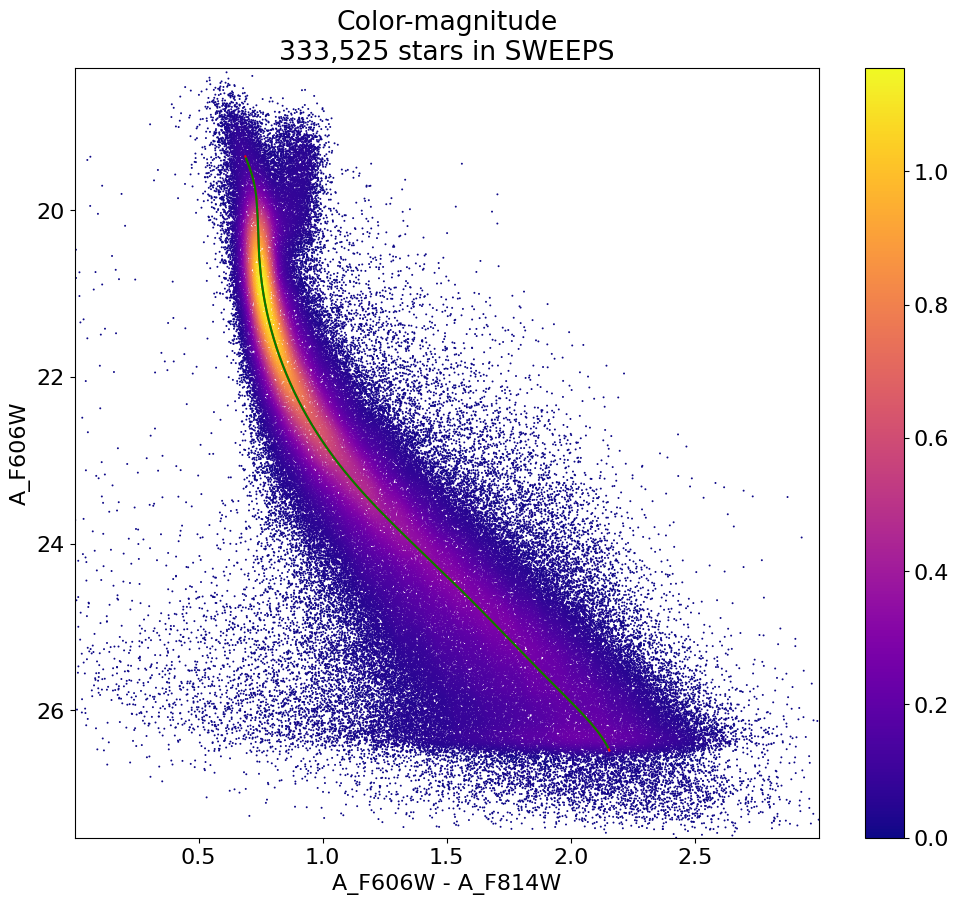
Plot the ridgeline on the CMD

fig, ax = plt.subplots(figsize=(12, 10))

sc = ax.scatter(xs, ys, c=zs, s=2, edgecolors='none', cmap='plasma')

# overplot ridge line
ax.plot(ridge_color(axes[1][wx]), axes[1][wx], color='red')
ax.plot(axes[0], ridge_mag(axes[0]), color='green')

ax.set(xlabel='A_F606W - A_F814W', ylabel='A_F606W',
       title=f'Color-magnitude\n{len(x):,} stars in SWEEPS',
       xlim=(xedge[0], xedge[-1]), ylim=(yedge[0], yedge[-1]))
ax.invert_yaxis()
_ = fig.colorbar(sc, ax=ax)

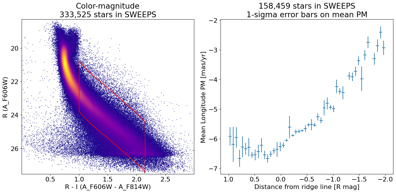
Binned distribution of PM(Long) vs magnitude offset from ridge line

yloc = ridge_mag(x)
x1 = x[np.isfinite(yloc)]
wy = np.where((axes[0] >= x1.min()) & (axes[0] <= x1.max()))[0]
ridgey = ridge_mag(axes[0][wy])

# Weighted histogram
dmagmin = -2.0
dmagmax = 1.0
xmax = axes[0][wy[-1]]
# xmin = axes[0][wy[0]]
xmin = 1.0
wsel = np.where((y-yloc >= dmagmin) & (y-yloc <= dmagmax) & (x >= xmin) & (x <= xmax))[0]

x2 = y[wsel]-yloc[wsel]
y2 = lpm[wsel]-lpm.mean()
hrange = (dmagmin, dmagmax)
hbins = 50
count1d, xedge1d = np.histogram(x2, range=hrange, bins=hbins)
lpm_sum1d = np.histogram(x2, range=hrange, bins=hbins, weights=y2)[0]
lpm_sumsq1d = np.histogram(x2, range=hrange, bins=hbins, weights=y2**2)[0]

ccount1d = count1d.clip(1)
lpm_mean1d = lpm_sum1d/ccount1d
lpm_rms1d = np.sqrt(lpm_sumsq1d/ccount1d-lpm_mean1d**2)
lpm_msigma1d = lpm_rms1d/np.sqrt(ccount1d)
lpm_mean1d += lpm.mean()

x1d = 0.5*(xedge1d[1:]+xedge1d[:-1])

xboundary = np.hstack((axes[0][wy], axes[0][wy[::-1]]))
yboundary = np.hstack((ridgey+dmagmax, ridgey[::-1]+dmagmin))
wb = np.where((xboundary >= xmin) & (xboundary <= xmax))
xboundary = xboundary[wb]
yboundary = yboundary[wb]
print(xboundary[0], yboundary[0], xboundary[-1], yboundary[-1])
print(xboundary.shape, yboundary.shape)
xboundary = np.append(xboundary, xboundary[0])
yboundary = np.append(yboundary, yboundary[0])

# don't plot huge error points
wp = np.where(lpm_msigma1d < 1)

1.0020693112164736 23.784969024110392 1.0020693112164736 20.784969024110392
(394,) (394,)

fig, (ax1, ax2) = plt.subplots(nrows=1, ncols=2, figsize=(14, 7), tight_layout=True)

ax1.scatter(xs, ys, c=zs, s=2, edgecolors='none', cmap='plasma')
ax1.plot(xboundary, yboundary, color='red')
ax1.set(xlabel='R - I (A_F606W - A_F814W)', ylabel='R (A_F606W)',
        title=f'Color-magnitude\n{len(x):,} stars in SWEEPS',
        xlim=(xedge[0], xedge[-1]), ylim=(yedge[0], yedge[-1]))
ax1.invert_yaxis()

ax2.errorbar(x1d[wp], lpm_mean1d[wp], xerr=(xedge1d[1]-xedge1d[0])/2.0, yerr=lpm_msigma1d[wp], linestyle='')
ax2.set(xlabel='Distance from ridge line [R mag]', ylabel='Mean Longitude PM [mas/yr]',
        title=f'{len(x2):,} stars in SWEEPS\n1-sigma error bars on mean PM')
ax2.invert_xaxis()

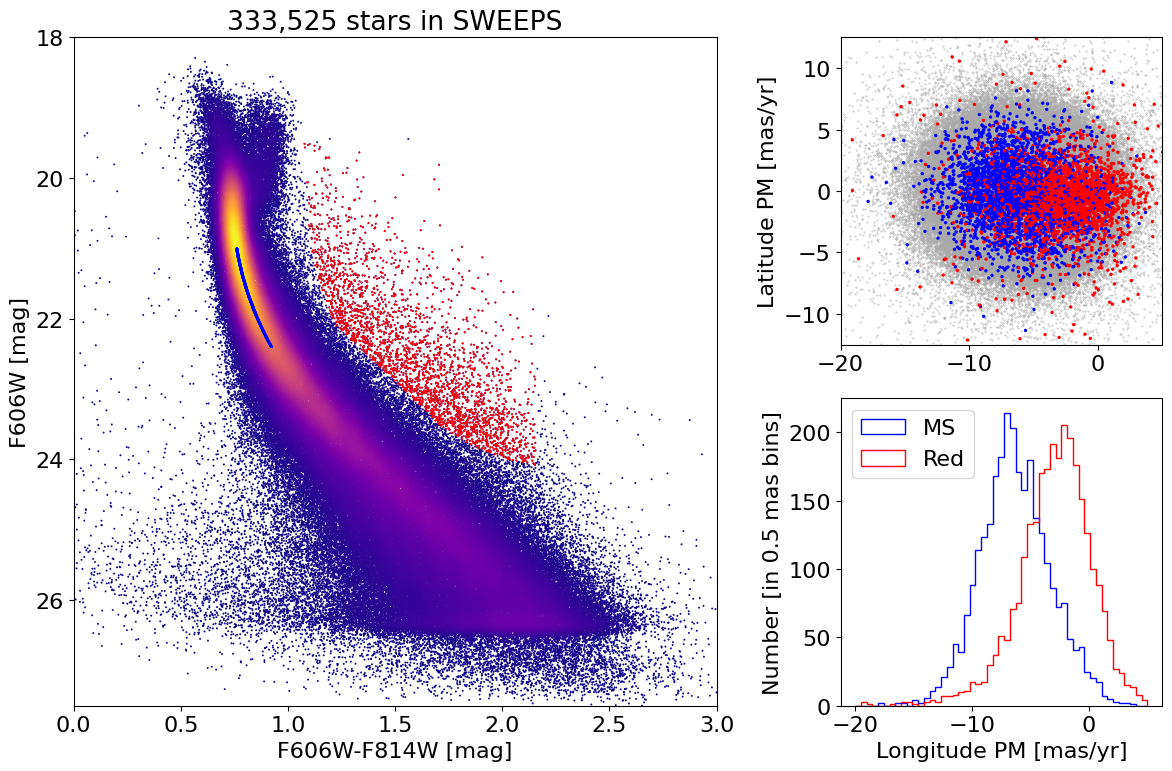
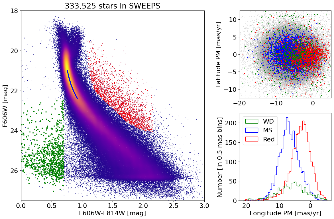
Reproduce Figure 1 from Calamida et al. 2014

w = np.where((RminusI > 0) & (RminusI < 3) & good)[0]

# Calculate the point density
x = np.array(RminusI[w])
y = np.array(f606w[w])
myPDF, axes = fastKDE.pdf(x, y, numPoints=2**10+1)
finterp = RectBivariateSpline(axes[1], axes[0], myPDF)
z = finterp(y, x, grid=False)
idx = z.argsort()
xs, ys, zs = x[idx], y[idx], z[idx]

# select a random subset of points in the most crowded regions to speed up plotting
wran = np.where(np.random.random(len(zs))*zs < 0.1)[0]
print(f"Plotting {len(wran)} of {len(zs)} points")
xs = xs[wran]
ys = ys[wran]
zs = zs[wran]

# locate ridge line in magnitude as a function of color
xloc = ridge_color(y)
ridgex = ridge_color(axes[1][wx])

# locate ridge line in color as function of magnitude
yloc = ridge_mag(x)
x1 = x[np.isfinite(yloc)]
wy = np.where((axes[0] >= x1.min()) & (axes[0] <= x1.max()))[0]
ridgey = ridge_mag(axes[0][wy])

# low-noise objects
print(f"Selected {len(w):,} low-noise objects")

# red objects
ylim = yloc - 1.5 - (yloc - 25.0).clip(0)/(1+10.0**(-0.4*(yloc-26.0)))
wred = np.where((y < 25) & (y > 19.5) & (y < ylim) & (x-xloc > 0.35))[0]
# wred = np.where((y<25) & (y > 19.5) & ((y-yloc) < -1.5)
#                   & (x-xloc > 0.3))[0]
#                   & (x > 1.1) & (x < 2.5) & (x-xloc > 0.2))[0]
print(f"Selected {len(wred):,} red objects")
# main sequence objects
wmain = np.where((y > 21) & (y < 22.4) & (np.abs(x-xloc) < 0.1))[0]
print(f"Initially selected {len(wmain):,} MS objects")
# sort by distance from ridge and select the closest
wmain = wmain[np.argsort(np.abs(x[wmain]-xloc[wmain]))]
wmain = wmain[:len(wred)]
print(f"Selected {len(wmain):,} MS objects closest to ridge")

Plotting 156044 of 333525 points
Selected 333,525 low-noise objects
Selected 2,797 red objects
Initially selected 59,605 MS objects
Selected 2,797 MS objects closest to ridge

fig = plt.figure(figsize=(12, 8), tight_layout=True)
gs = gridspec.GridSpec(2, 2, width_ratios=[2, 1])

ax1 = fig.add_subplot(gs[:, 0])
ax2 = fig.add_subplot(gs[0, 1])
ax3 = fig.add_subplot(gs[1, 1])

# plot ax1
ax1.scatter(xs, ys, c=zs, s=2, cmap='plasma', edgecolors='none')
ax1.scatter(x[wred], y[wred], c='red', s=2, edgecolors='none')
ax1.scatter(x[wmain], y[wmain], c='blue', s=2, edgecolors='none')
ax1.set(xlabel='F606W-F814W [mag]', ylabel='F606W [mag]', title=f'{len(x):,} stars in SWEEPS',
        xlim=(0, 3), ylim=(18, 27.5))
ax1.invert_yaxis()

# plot ax2
lrange = (-20, 5)
brange = (-12.5, 12.5)

# MS and red points in random order
wsel = w[np.append(wmain, wred)]
colors = np.array(['blue']*len(wsel))
colors[len(wmain):] = 'red'
irs = np.argsort(np.random.random(len(wsel)))
wsel = wsel[irs]
colors = colors[irs]

masks = [w, wsel]
sizes = [0.1, 2]
colors2 = ['darkgray', colors]

for mask, color, size in zip(masks, colors2, sizes):
    ax2.scatter('lpm', 'bpm', data=tab[mask], c=color, s=size)

ax2.set(ylabel='Latitude PM [mas/yr]', xlim=lrange, ylim=brange)

# plot ax3
bins = 0.5
bincount = int((lrange[1]-lrange[0])/bins + 0.5) + 1

masks = [w[wmain], w[wred]]
labels = ['MS', 'Red']
colors = ['b', 'r']

for mask, label, color in zip(masks, labels, colors):
    ax3.hist('lpm', data=tab[mask], range=lrange, bins=bincount, label=label, color=color, histtype='step')

ax3.set(xlabel='Longitude PM [mas/yr]', ylabel=f'Number [in {bins:.2} mas bins]')
_ = ax3.legend(loc='upper left')

Mean and median proper motions of bulge stars compared with SgrA*

(-6.379 \(\pm\) 0.026, -0.202 \(\pm\) 0.019) mas/yr Reid and Brunthaler (2004)

lpmmain = np.mean(tab['lpm'][w[wmain]])
bpmmain = np.mean(tab['bpm'][w[wmain]])

norm = 1.0/np.sqrt(len(tab['lpm'][w[wmain]]))
print("Bulge stars mean PM longitude {:.2f} +- {:.3f} latitude {:.2f} +- {:.3f}".format(
    np.mean(tab['lpm'][w[wmain]]), norm*np.std(tab['lpm'][w[wmain]]),
    np.mean(tab['bpm'][w[wmain]]), norm*np.std(tab['bpm'][w[wmain]])
    ))

norm = 1.2533/np.sqrt(len(tab['lpm'][w[wmain]]))
print("Bulge stars median PM longitude {:.2f} +- {:.3f} latitude {:.2f} +- {:.3f}".format(
    np.median(tab['lpm'][w[wmain]]), norm*np.std(tab['lpm'][w[wmain]]),
    np.median(tab['bpm'][w[wmain]]), norm*np.std(tab['bpm'][w[wmain]])
    ))

Bulge stars mean PM longitude -6.31 +- 0.059 latitude -0.13 +- 0.053
Bulge stars median PM longitude -6.45 +- 0.074 latitude -0.13 +- 0.067

White Dwarfs

w = np.where((RminusI > 0) & (RminusI < 3) & good)[0]

wwd = np.where((RminusI < 0.7)
               & (RminusI > 0) 
               & (f606w > 22.5) 
               & good 
               & (tab['lpm'] < 5) 
               & (tab['lpm'] > -20))[0]
xwd = np.array(RminusI[wwd])
ywd = np.array(f606w[wwd])

# Calculate the point density
x = np.array(RminusI[w])
y = np.array(f606w[w])

myPDF, axes = fastKDE.pdf(x, y, numPoints=2**10+1)
finterp = RectBivariateSpline(axes[1], axes[0], myPDF)
z = finterp(y, x, grid=False)
idx = z.argsort()
xs, ys, zs = x[idx], y[idx], z[idx]

# select a random subset of points in the most crowded regions to speed up plotting
wran = np.where(np.random.random(len(zs))*zs < 0.1)[0]
print(f"Plotting {len(wran)} of {len(zs)} points")
xs = xs[wran]
ys = ys[wran]
zs = zs[wran]

# locate ridge line in magnitude as a function of color
xloc = ridge_color(y)
ridgex = ridge_color(axes[1][wx])

# locate ridge line in color as function of magnitude
yloc = ridge_mag(x)
x1 = x[np.isfinite(yloc)]
wy = np.where((axes[0] >= x1.min()) & (axes[0] <= x1.max()))[0]
ridgey = ridge_mag(axes[0][wy])

# low-noise objects
print(f"Selected {len(w):,} low-noise objects")

# red objects
ylim = yloc - 1.5 - (yloc - 25.0).clip(0)/(1+10.0**(-0.4*(yloc-26.0)))
wred = np.where((y < 25) & (y > 19.5) & (y < ylim) & (x-xloc > 0.35))[0]
# wred = np.where((y < 25) & (y > 19.5) & ((y-yloc) < -1.5)
#                   & (x-xloc > 0.3))[0]
#                   & (x > 1.1) & (x < 2.5) & (x-xloc > 0.2))[0]
print("Selected {:,} red objects".format(len(wred)))
# main sequence objects
wmain = np.where((y > 21) & (y < 22.4) & (np.abs(x-xloc) < 0.1))[0]
print("Initially selected {:,} MS objects".format(len(wmain)))
# sort by distance from ridge and select the closest
wmain = wmain[np.argsort(np.abs(x[wmain]-xloc[wmain]))]
wmain = wmain[:len(wred)]
print(f"Selected {len(wmain):,} MS objects closest to ridge")

Plotting 156416 of 333525 points
Selected 333,525 low-noise objects
Selected 2,797 red objects
Initially selected 59,605 MS objects
Selected 2,797 MS objects closest to ridge

fig = plt.figure(figsize=(12, 8), tight_layout=True)
gs = gridspec.GridSpec(2, 2, width_ratios=[2, 1])

ax1 = fig.add_subplot(gs[:, 0])
ax2 = fig.add_subplot(gs[0, 1])
ax3 = fig.add_subplot(gs[1, 1])

# plot ax1
ax1.scatter(xs, ys, c=zs, s=2, cmap='plasma', edgecolors='none')
ax1.scatter(x[wred], y[wred], c='red', s=2, edgecolors='none')
ax1.scatter(x[wmain], y[wmain], c='blue', s=2, edgecolors='none')
ax1.scatter(xwd, ywd, c='green', s=10, edgecolors='none')
ax1.set(xlabel='F606W-F814W [mag]', ylabel='F606W [mag]',
        title=f'{len(x):,} stars in SWEEPS', xlim=(0, 3), ylim=(18, 27.5))
ax1.invert_yaxis()

# plot ax2
lrange = (-20, 5)
brange = (-12.5, 12.5)

# MS and red points in random order
wsel = w[np.append(wmain, wred)]
colors = np.array(['blue']*len(wsel))
colors[len(wmain):] = 'red'
irs = np.argsort(np.random.random(len(wsel)))
wsel = wsel[irs]
colors = colors[irs]

masks = [w, wsel, wwd]
sizes = [0.1, 2, 2]
colors2 = ['darkgray', colors, 'green']

for mask, color, size in zip(masks, colors2, sizes):
    ax2.scatter('lpm', 'bpm', data=tab[mask], c=color, s=size)

ax2.set(ylabel='Latitude PM [mas/yr]', xlim=lrange, ylim=brange)

# plot ax3
bins = 0.5
bincount = int((lrange[1]-lrange[0])/bins + 0.5) + 1

masks = [wwd, w[wmain], w[wred]]
labels = ['WD', 'MS', 'Red']
colors = ['g', 'b', 'r']

for mask, label, color in zip(masks, labels, colors):
    ax3.hist('lpm', data=tab[mask], range=lrange, bins=bincount, label=label, color=color, histtype='step')

ax3.set(xlabel='Longitude PM [mas/yr]', ylabel=f'Number [in {bins:.2} mas bins]')
_ = ax3.legend(loc='upper left')

White dwarf mean PM and uncertainity

norm = 1.0/np.sqrt(len(tab['lpm'][wwd]))
print("WD PM mean +- stdev longitude {:.2f} +- {:.3f} latitude {:.2f} +- {:.3f}".format(
    np.mean(tab['lpm'][wwd]), norm*np.std(tab['lpm'][wwd]),
    np.mean(tab['bpm'][wwd]), norm*np.std(tab['bpm'][wwd])
    ))

WD PM mean +- stdev longitude -5.60 +- 0.152 latitude -0.03 +- 0.245

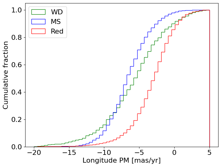
WDs generally closer to bulge (MS) PM distribution

bins = 0.5
bincount = int((lrange[1]-lrange[0])/bins + 0.5) + 1

masks = [wwd, w[wmain], w[wred]]
labels = ['WD', 'MS', 'Red']
colors = ['g', 'b', 'r']

fig, ax = plt.subplots(figsize=(8, 6))

for mask, label, color in zip(masks, labels, colors):
    ax.hist('lpm', data=tab[mask], range=lrange, bins=bincount, label=label, color=color, histtype='step', density=True, cumulative=1)
    
ax.set(xlabel='Longitude PM [mas/yr]', ylabel='Cumulative fraction')
_ = ax.legend(loc='upper left')

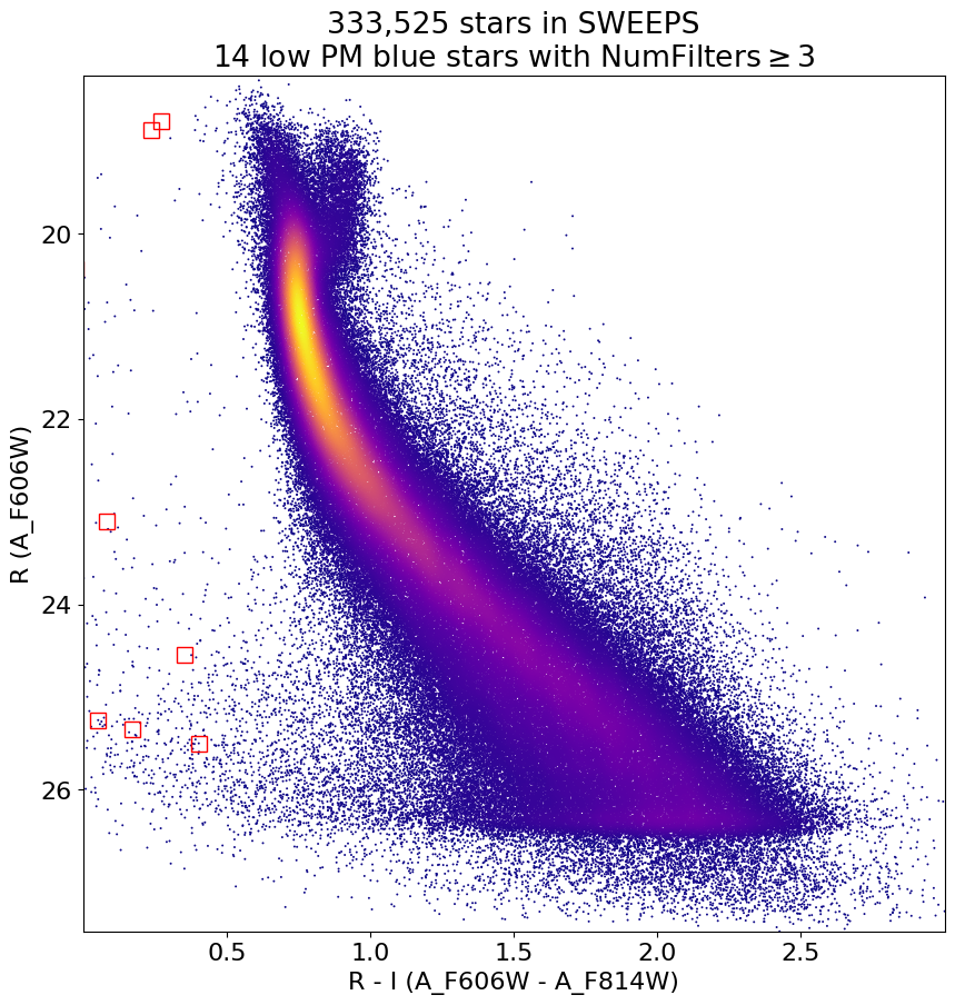
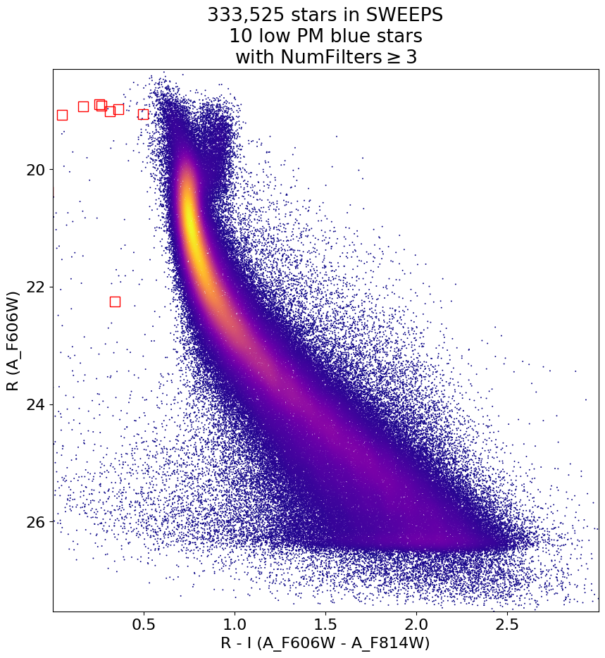
Look for quasar candidates (low PM blue stars)

Note this includes all objects, not just “good” objects with low mag noise, because quasars might be variable too.

wqso1 = np.where((RminusI < 0.5)
                 & (np.sqrt(tab['bpm']**2+tab['lpm']**2) < 1.0)
                 & (tab['NumFilters'] > 2))[0]
wqso1 = wqso1[np.argsort(f606w[wqso1])]
tab[wqso1]

Table length=14

ObjID	RA	Dec	RAerr	Decerr	NumFilters	NumVisits	a_f606w	a_f606w_n	a_f606w_mad	a_f814w	a_f814w_n	a_f814w_mad	bpm	lpm	bpmerr	lpmerr	pmdev	yr	dT	yrStart	yrEnd
int64	float64	float64	float64	float64	int32	int32	float64	int32	float64	float64	int32	float64	float64	float64	float64	float64	float64	float64	float64	float64	float64
4000710313439	269.74005171773325	-29.196032473369662	0.6265964047671119	0.8430363739939153	13	94	18.632399559020996	74	0.04414939880371094	18.75860023498535	77	0.22760009765625	-0.2729591957006581	0.0933685295161405	0.12007496779671313	0.19354443197999766	6.664561102885139	2010.4104580987043	12.138936292937231	2003.436727359001	2015.5756636519384
4000710257520	269.76634477578085	-29.223310166797457	0.7010607226863969	0.9635875312674559	14	96	18.71660041809082	75	0.03790092468261719	18.785300254821777	74	0.45225048065185547	-0.579616612423514	-0.004195674864531432	0.1286260805301132	0.22613515613212812	7.079734373347017	2010.4505865929348	12.138936292937231	2003.436727359001	2015.5756636519384
4000710307965	269.7417955221381	-29.198593859432016	0.9205935728204635	0.8518786138892231	14	94	18.73979949951172	73	0.06389999389648438	18.865349769592285	76	0.20005035400390625	0.3782536664095988	-0.3686895590223385	0.2125072995299893	0.17345047912667094	7.6732306607203995	2010.485877546229	12.138936292937231	2003.436727359001	2015.5756636519384
4000710352240	269.7337926320315	-29.18139487545298	0.6946356814006966	0.9061342261773224	4	79	18.78339958190918	74	0.023049354553222656	18.512550354003906	74	0.2772502899169922	0.6337179460443223	0.29715583737809054	0.15063272942700434	0.20070198442295878	6.738108122324751	2009.7737370001337	11.371185208171667	2003.436727359001	2014.8079125671727
4000710347699	269.7783405856686	-29.17911931116647	0.41155778832388173	0.4841933620053226	4	81	18.839149475097656	76	0.0339508056640625	18.898500442504883	73	0.23670005798339844	-0.11678100312847553	0.6499252564776745	0.084877817774843	0.11036052576232969	3.7905072891090166	2009.7600421422271	11.371185208171667	2003.436727359001	2014.8079125671727
4000710305789	269.7500895465239	-29.199706962876274	1.2377985340299074	0.9596173093379398	13	95	18.883800506591797	76	0.016399383544921875	18.647899627685547	75	0.10449981689453125	0.7613608897396442	0.06072801567912481	0.14458519679206283	0.307891087664392	8.669608674616846	2010.4513188181218	12.138936292937231	2003.436727359001	2015.5756636519384
4000710287023	269.73049137354224	-29.208786514685837	0.5886781414210673	0.8187862653505924	13	93	19.005799293518066	70	0.17949867248535156	19.03809928894043	77	0.4453010559082031	-0.027042326411294833	-0.10656181801795192	0.11368759414535684	0.18547384893472832	6.060019340850642	2010.4099808141818	12.138936292937231	2003.436727359001	2015.5756636519384
4000711198572	269.7837898799627	-29.171058346187387	0.24289061146320284	0.3787994581356928	4	56	20.384400367736816	52	0.030750274658203125	20.409199714660645	54	0.018199920654296875	-0.39276687371980523	-0.2614991280329616	0.07157257977281026	0.06954852374618407	2.6397832644001498	2008.0522535045122	10.997621905233284	2003.436727359001	2014.4343492642342
4000711114267	269.77699533206413	-29.213020339932903	4.24137055513596	3.9397646738783108	4	35	23.104300498962402	32	0.038299560546875	23.02050018310547	33	0.07789993286132812	-0.8306962177406612	-0.06858498728152404	0.9221622324872899	1.3496664163664274	18.925994277649572	2005.5542194355585	12.136400136689947	2003.436727359001	2015.573127495691
4000710335454	269.7613531455845	-29.187206361070864	7.474297329875963	1.4831362310495328	3	77	23.993050575256348	76	0.06319999694824219	24.481599807739258	79	0.20109939575195312	-0.5423185685515735	0.7060415611802732	1.4646930044718638	0.8183749010089348	44.542864374423985	2009.9793326372383	11.371185208171667	2003.436727359001	2014.8079125671727
4000710273567	269.7541240409338	-29.21578796024474	4.748214164796449	1.6940945228632924	3	78	24.544499397277832	76	0.07555007934570312	24.190000534057617	78	0.12094974517822266	-0.06045787883823814	-0.29699839716096693	0.9328189717625861	0.5780921890931368	28.400690195232727	2009.6896657994198	11.341399291029212	2003.436727359001	2014.7781266500303
4000710273213	269.762844233717	-29.215993073596458	2.8491412759641146	2.1589511176356435	3	58	25.248699188232422	57	0.072601318359375	25.19580078125	57	0.11439895629882812	0.5874532592404308	0.3961988878194328	0.5745702330625071	0.4892686278049602	17.035022816134603	2008.6575729055041	11.371185208171667	2003.436727359001	2014.8079125671727
4000710327380	269.7667196275462	-29.189803905653022	1.4975661577032107	4.6584789458436155	3	53	25.343299865722656	52	0.09395027160644531	25.171499252319336	35	0.27519989013671875	-0.5925764852209691	0.3510984622430878	0.40036043056387555	0.963110172251642	23.394971123121124	2008.1998409952648	11.341399291029212	2003.436727359001	2014.7781266500303
4000710296308	269.7744892710409	-29.20439243403908	3.8554370972569254	2.2643903195117683	3	78	25.49880027770996	75	0.09670066833496094	25.095499992370605	78	0.11275005340576172	0.18975302378694214	0.17171660653658127	0.7173616133509608	0.6443087550732374	27.184284641221293	2009.575015347384	11.371732905164137	2003.4361796620085	2014.8079125671727

fig, ax = plt.subplots(figsize=(10, 10))
ax.scatter(xs, ys, c=zs, s=2, edgecolors='none', cmap='plasma')
ax.plot(RminusI[wqso1], f606w[wqso1], 'rs', markersize=10, fillstyle='none')
ax.set(xlim=(xedge[0], xedge[-1]), ylim=(yedge[0], yedge[-1]))
ax.set(xlabel='R - I (A_F606W - A_F814W)', ylabel='R (A_F606W)',
       title=f'{len(x):,} stars in SWEEPS\n{len(wqso1)} low PM blue stars with NumFilters$\\geq3$')
ax.invert_yaxis()

objid = tab['ObjID']
print(f"Plotting {len(wqso1)} objects")
for o in objid[wqso1]:
    positions(o, jobs=jobs)

Plotting 14 objects

Try again with different criteria on proper motion fit quality

wqso2 = np.where((RminusI < 0.5)
                 & (np.sqrt(tab['bpm']**2+tab['lpm']**2) < 2.0)
                 & (np.sqrt(tab['bpmerr']**2+tab['lpmerr']**2) < 2.0)
                 & (tab['pmdev'] < 4.0))[0]
wqso2 = wqso2[np.argsort(f606w[wqso2])]
tab[wqso2]

Table length=10

ObjID	RA	Dec	RAerr	Decerr	NumFilters	NumVisits	a_f606w	a_f606w_n	a_f606w_mad	a_f814w	a_f814w_n	a_f814w_mad	bpm	lpm	bpmerr	lpmerr	pmdev	yr	dT	yrStart	yrEnd
int64	float64	float64	float64	float64	int32	int32	float64	int32	float64	float64	int32	float64	float64	float64	float64	float64	float64	float64	float64	float64	float64
4000710347699	269.7783405856686	-29.17911931116647	0.41155778832388173	0.4841933620053226	4	81	18.839149475097656	76	0.0339508056640625	18.898500442504883	73	0.23670005798339844	-0.11678100312847553	0.6499252564776745	0.084877817774843	0.11036052576232969	3.7905072891090166	2009.7600421422271	11.371185208171667	2003.436727359001	2014.8079125671727
4000711253077	269.6915378419676	-29.24020145019322	0.4704881733739859	0.5270162975364242	2	46	18.8927001953125	45	0.010900497436523438	18.636449813842773	42	0.1782999038696289	-1.7408991354864214	-0.5947077102632641	0.3613162305972112	0.7482345212707299	2.9613403618906435	2013.5034009429392	3.00678120252487	2011.8016761776817	2014.8084573802066
4000711347522	269.70065127433986	-29.232034952664744	0.45813739460650355	0.972550620957754	2	43	18.917999267578125	43	0.025800704956054688	18.648849487304688	38	0.2850008010864258	0.5245222694829835	-0.9025321571402278	0.5331879231467277	1.1329901624612693	3.7307809424771032	2013.4648969161435	3.00678120252487	2011.8016761776817	2014.8084573802066
4000709025473	269.82873131529516	-29.19512257484812	0.5411363937542479	0.6920450307671305	2	46	18.92685031890869	44	0.0126495361328125	18.75755023956299	42	0.3887491226196289	0.8548976473145768	-1.1578337695544032	0.2876906708357735	0.43355270853508593	3.456340262841035	2013.315425703565	11.371914541371764	2003.4361796620085	2014.8080942033803
4000710279756	269.7207706977463	-29.212308555948887	0.41374484392259747	0.4883003181612267	12	70	18.977749824523926	54	0.028249740600585938	18.614700317382812	55	0.3589000701904297	0.033714894109117335	-1.600702228805833	0.09052420732956741	0.09073750139459606	3.619701382694334	2009.679762289423	12.138936292937231	2003.436727359001	2015.5756636519384
4000711345953	269.71277619272627	-29.23130608012401	0.4732191836487131	1.0046856684238223	2	46	19.01865005493164	46	0.012249946594238281	18.701799392700195	39	0.1501007080078125	0.34968560305135327	1.9139934804091387	0.7254248849571668	1.0861879082833583	3.755315552645739	2013.5034009429392	3.00678120252487	2011.8016761776817	2014.8084573802066
4000709014231	269.8069522092499	-29.20021994406481	0.3834521659779482	0.549067011791737	2	47	19.06329917907715	46	0.037700653076171875	18.564849853515625	46	0.046050071716308594	1.0342947783087193	-1.4279240765589876	0.15526546888889428	0.36889847542727655	2.0017413819595076	2013.3007902147058	11.371914541371764	2003.4361796620085	2014.8080942033803
4000710326758	269.75587447129374	-29.189995188046638	0.39923238020201557	0.37137690294128917	13	95	19.077000617980957	76	0.021599769592285156	19.024099349975586	77	0.26650047302246094	-1.1141957269870415	-0.8674983559009859	0.09948022058874997	0.06424053625731577	3.097878914716658	2010.4513188181215	12.138936292937231	2003.436727359001	2015.5756636519384
4000711198572	269.7837898799627	-29.171058346187387	0.24289061146320284	0.3787994581356928	4	56	20.384400367736816	52	0.030750274658203125	20.409199714660645	54	0.018199920654296875	-0.39276687371980523	-0.2614991280329616	0.07157257977281026	0.06954852374618407	2.6397832644001498	2008.0522535045122	10.997621905233284	2003.436727359001	2014.4343492642342
4000724763944	269.7747901164537	-29.26523403383687	0.43377673171406406	0.4474216647110866	2	46	22.25380039215088	46	0.05949974060058594	21.910449981689453	46	0.033699989318847656	1.182122334720074	0.14084928991004503	0.5960881587431285	0.4264522488795796	3.3639208538613516	2013.503145357016	3.00678170959782	2011.801494066038	2014.8082757756358

fig, ax = plt.subplots(figsize=(10, 10))
ax.scatter(xs, ys, c=zs, s=2, edgecolors='none', cmap='plasma')
ax.plot(RminusI[wqso2], f606w[wqso2], 'rs', markersize=10, fillstyle='none')
ax.set(xlabel='R - I (A_F606W - A_F814W)', ylabel='R (A_F606W)',
       xlim=(xedge[0], xedge[-1]), ylim=(yedge[0], yedge[-1]),
       title=f'{len(x):,} stars in SWEEPS\n{len(wqso2)} low PM blue stars\nwith NumFilters$\\geq3$')
ax.invert_yaxis()

objid = tab['ObjID']
print(f"Plotting {len(wqso2)} objects")
for o in objid[wqso2]:
    positions(o, jobs=jobs)

Plotting 10 objects

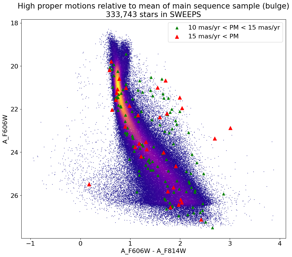
High Proper Motion Objects

Get a list of objects with high, accurately measured proper motions. Proper motions are measured relative to the main sequence sample (Galactic center approximately).

f606w = tab['a_f606w']
f814w = tab['a_f814w']
RminusI = f606w-f814w
lpm0 = np.array(tab['lpm'])
bpm0 = np.array(tab['bpm'])
lpmerr0 = np.array(tab['lpmerr'])
bpmerr0 = np.array(tab['bpmerr'])
pmtot0 = np.sqrt((bpm0-bpmmain)**2+(lpm0-lpmmain)**2)
pmerr0 = np.sqrt(bpmerr0**2+lpmerr0**2)

# sort samples by decreasing PM
wpml = np.where((pmtot0 > 12) & (pmtot0 < 15) & (pmerr0 < 1.0) & good)[0]
wpml = wpml[np.argsort(-pmtot0[wpml])]
xpml = np.array(RminusI[wpml])
ypml = np.array(f606w[wpml])

wpmh = np.where((pmtot0 > 15) & (pmerr0 < 1.0) & good)[0]
wpmh = wpmh[np.argsort(-pmtot0[wpmh])]
xpmh = np.array(RminusI[wpmh])
ypmh = np.array(f606w[wpmh])

# Calculate the point density
w = np.where((RminusI > -1) & (RminusI < 4) & good)[0]
x = np.array(RminusI[w])
y = np.array(f606w[w])
t0 = time.time()
myPDF, axes = fastKDE.pdf(x, y, numPoints=2**10+1)
print(f"kde took {(time.time()-t0):.1f} sec")

# interpolate to get z values at points
finterp = RectBivariateSpline(axes[1], axes[0], myPDF)
z = finterp(y, x, grid=False)

# Sort the points by density, so that the densest points are plotted last
idx = z.argsort()
xs, ys, zs = x[idx], y[idx], z[idx]

# select a random subset of points in the most crowded regions to speed up plotting
wran = np.where(np.random.random(len(zs))*zs < 0.05)[0]
print(f"Plotting {len(wran)} of {len(zs)} points")
xs = xs[wran]
ys = ys[wran]
zs = zs[wran]

kde took 1.4 sec

Plotting 98616 of 333743 points

fig, ax = plt.subplots(figsize=(12, 10))

ax.scatter(xs, ys, c=zs, s=2, edgecolors='none', cmap='plasma')
ax.scatter(xpml, ypml, s=40, c="green", marker="^", label='10 mas/yr < PM < 15 mas/yr')
ax.scatter(xpmh, ypmh, s=80, c="red", marker="^", label='15 mas/yr < PM')

ax.set(xlabel='A_F606W - A_F814W', ylabel='A_F606W',
       title=f'High proper motions relative to mean of main sequence sample (bulge)\n{len(x):,} stars in SWEEPS')

ax.invert_yaxis()
ax.legend()

<matplotlib.legend.Legend at 0x7f3fa5605ed0>

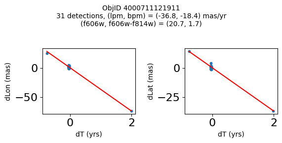
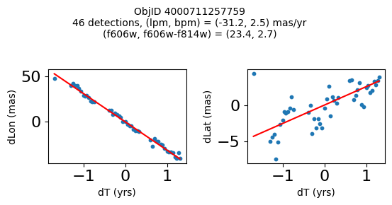
print(f"Plotting {len(wpmh)} objects")
for o in tab["ObjID"][wpmh]:
    positions(o, jobs=jobs)

Plotting 34 objects

Very red high proper motion objects

wpmred =  np.where((pmtot0 > 12) & (pmerr0 < 1.0) & (RminusI > 2.6) & good)[0]
print(f"Plotting {len(wpmred)} objects")
for o in tab["ObjID"][wpmred]:
    positions(o, jobs=jobs)

Plotting 4 objects

Very blue high proper motion objects

wpmblue =  np.where((pmtot0 > 8) & (pmerr0 < 1.0) & (RminusI < 0.5) & good)[0]
print(f"Plotting {len(wpmblue)} objects")
for o in tab["ObjID"][wpmblue]:
    positions(o, jobs=jobs)

Plotting 12 objects

Get HLA cutout images for selected objects

Get HLA color cutout images for the high-PM objects. The query_hla function gets a table of all the color images that are available at a given position using the f814w+f606w filters. The get_image function reads a single cutout image (as a JPEG color image) and returns a PIL image object.

See the documentation on HLA VO services and the fitscut image cutout service for more information on the web services being used.

def query_hla(ra, dec, size=0.0, imagetype="color", inst="ACS", format="image/jpeg",
              spectral_elt=("f814w", "f606w"), autoscale=95.0, asinh=1, naxis=33):
    # convert a list of filters to a comma-separated string
    if not isinstance(spectral_elt, str):
        spectral_elt = ",".join(spectral_elt)
    siapurl = (f"https://hla.stsci.edu/cgi-bin/hlaSIAP.cgi?"
               f"pos={ra},{dec}&size={size}&imagetype={imagetype}&inst={inst}"
               f"&format={format}&spectral_elt={spectral_elt}"
               f"&autoscale={autoscale}&asinh={asinh}"
               f"&naxis={naxis}")
    votable = Table.read(siapurl, format="votable")
    return votable


def get_image(url):
    """Get image from a URL"""
    r = requests.get(url)
    im = Image.open(BytesIO(r.content))
    return im

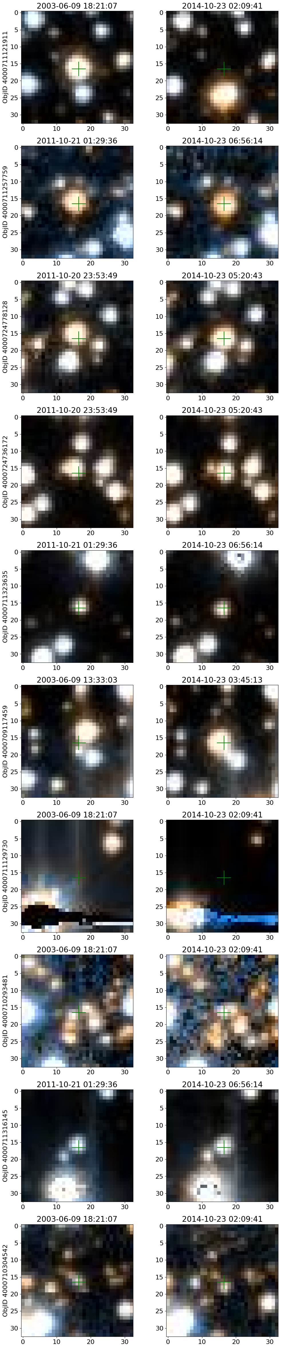
# display earliest and latest images side-by-side
# wsel = wpmred
# wsel = wpmblue
# top 10 highest PM objects
wsel = wpmh[:10]
nim = len(wsel)
icols = 1        # objects per row
ncols = 2*icols  # two images for each object
nrows = (nim+icols-1)//icols

imsize = 33
xcross = np.array([-1, 1, 0, 0, 0])*2 + imsize/2
ycross = np.array([0, 0, 0, -1, 1])*2 + imsize/2

# selected data from tab
sd = tab[['RA', 'Dec', 'ObjID']][wsel]

# create the figure
fig, axes = plt.subplots(nrows=nrows, ncols=ncols, figsize=(12, (12/ncols)*nrows))

# iterate each observation, and each set of axes for the first and last image
for (ax1, ax2), obj in zip(axes, sd):
    
    # get the image urls and observation datetime
    hlatab = query_hla(obj["RA"], obj["Dec"], naxis=imsize)[['URL', 'StartTime']]
    # sort the data by the observation datetime, and get the first and last observation url
    (url1, time1), (url2, time2) = hlatab[np.argsort(hlatab['StartTime'])][[0, -1]]
    
    # get the images
    im1 = get_image(url1)
    im2 = get_image(url2)
    
    # plot the images
    ax1.imshow(im1, origin="upper")
    ax2.imshow(im2, origin="upper")
    
    # plot the center
    ax1.plot(xcross, ycross, 'g')
    ax2.plot(xcross, ycross, 'g')
    
    # labels and titles
    ax1.set(ylabel=f'ObjID {obj["ObjID"]}', title=time1)
    ax2.set_title(time2)

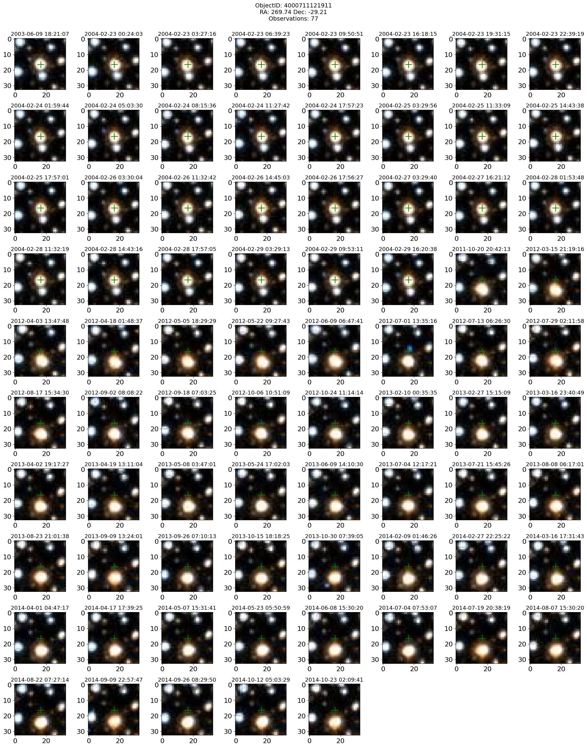
Look at the entire collection of images for the highest PM object

i = wpmh[0]

# selected data
sd = tab['ObjID', 'RA', 'Dec', 'a_f606w', 'a_f814w', 'bpm', 'lpm', 'yr', 'dT'][i]
display(sd)

imsize = 33
# get the URL and StartTime data
hlatab = query_hla(sd['RA'], sd['Dec'], naxis=imsize)[['URL', 'StartTime']]
# sort the data
hlatab = hlatab[np.argsort(hlatab['StartTime'])]

nim = len(hlatab)
ncols = 8
nrows = (nim+ncols-1)//ncols

xcross = np.array([-1, 1, 0, 0, 0])*2 + imsize/2
ycross = np.array([0, 0, 0, -1, 1])*2 + imsize/2

Row index=208405

ObjID	RA	Dec	a_f606w	a_f814w	bpm	lpm	yr	dT
int64	float64	float64	float64	float64	float64	float64	float64	float64
4000711121911	269.7367256594695	-29.209699919117618	20.67275047302246	18.963199615478516	-18.43788346257518	-36.80145933087569	2004.194238143401	2.749260607770275

# get the images: takes about 90 seconds for 77 images
images = [get_image(url) for url in hlatab['URL']]

# create the figure
fig, axes = plt.subplots(nrows=nrows, ncols=ncols, figsize=(20, (20/ncols)*nrows), tight_layout=True)
# flatten the axes for easy iteration and zipping
axes = axes.flat

plt.rcParams.update({"font.size": 11})
for ax, time1, img in zip(axes, hlatab['StartTime'], images):
    # plot image
    ax.imshow(img, origin="upper")
    # plot the center
    ax.plot(xcross, ycross, 'g')
    # set the title
    ax.set_title(time1)
    
# remove the last 3 unused axes
for ax in axes[nim:]:
    ax.remove()

_ = fig.suptitle(f"ObjectID: {sd['ObjID']}\nRA: {sd['RA']:0.2f} Dec: {sd['Dec']:0.2f}\nObservations: {nim}", y=1, fontsize=14)