
JWST SI Keyword Search for Exoplanet Spectra#
Introduction#
This tutorial will illustrate how to use the MAST API to search for JWST science data by values of FITS header keywords, and then retrieve all products for the corresponding observations.
Searching by SI Keyword values and accessing all data products is not supported in the MAST Portal, nor with the astroquery.mast Observations class by itself. Rather, we will be using astroquery.mast’s Mast class to make direct calls to the MAST API.
Specifically, this tutorial will show you how to:
Use the
Mastclass of astroquery.mast to search for JWST science files by values of FITS header keywordsConstruct a unique set of Observation IDs to perform a search with the astroquery.mast
ObservationclassFetch the unique data products associated with the Observations
Filter the results for science products
Download a bash script to retrieve the filtered products
- Advanced Search for Observations: Uses the
Observationsclass to search for data products that match certain metadata values. The available metadata upon which to conduct such a search is limited to coordinates, timestamps, and a modest set of instrument configuration information. Returns MASTObservationsobjects, which are collections of all levels of products (all formats) and all ancillary data products. - SI Keyword Search: Uses the
Mastclass to search for FITS products that match values of user-specified keywords, where the set of possible keywords is very large. Returns only FITS products, and only finds highest level of calibrated products (generally, L-2b and L-3).
Connecting files that match keyword values to observations is not difficult, but it is a little convoluted. First, you’ll use the API to perform a Science Instrument (SI) Keyword Search to find matching product files. The names of these files contain the MAST Observation ID as a sub-string. Then we can use the IDs to perform an advanced Observation search for matching Observations.
Here are the steps in the process:
Part I: Keyword Search for Exoplanet Spectra
Part II: Convert to Observation Search Part III: Download Data Products Additional ResourcesImports#
The following packages are needed for this tutorial:
astropy.io allows us to open the
.fitsfiles that we downloadastropy.table holds the results of our product query and finds the unique files
astropy.time creates
Timeobjects and converts between time representationsastroquery.mast constructs the queries, retrieves tables of results, and retrieves data products
matplotlib.pyplot is a common plotting tool that we’ll use to look at our results
from astropy.io import fits
from astropy.table import unique, vstack
from astropy.time import Time
from astroquery.mast import Mast, Observations

import matplotlib.pyplot as plt
I : Keyword Search for Exoplanet Spectra#
This example shows how to search for NIRISS spectral time-series observations (TSO) taken of transiting exo-planets. The data are from Commissioning or Early Release Science programs, and are therefore public.
Specify Search Criteria#
The criteria for SI Keyword searches consists of FITS header keyword name/value pairs. Learn more about SI keywords from the JWST Keyword Dictionary, and about the supported set of keyword values that can be queried. With this kind of query it is necessary to construct a specific structure to hold the query parameters.
The following helper routines translate a simple dictionary (one that is easy to customize in Python) to the required JSON-style syntax, while the second creates a Min:Max pair of parameters for date-time stamps which, as with all parameters that vary continuously, must be expressed as a range of values in a dictionary.
def set_params(parameters):
    return [{"paramName": p, "values": v} for p, v in parameters.items()]


def set_mjd_range(min, max):
    '''Set time range in MJD given limits expressed as ISO-8601 dates'''
    return {
        "min": Time(min, format='isot').mjd,
        "max": Time(max, format='isot').mjd
        }
Add a Date Range#
A date range is specified here (though is not strictly needed) to illustrate how to express these common parameters. For historical reasons, the astroquery.mast parameter names for timestamps come in pairs: one with a similar name to the corresponding FITS keyword (e.g. data_obs), and another with the string _mjd appended (e.g. date_obs_mjd). The values are equivalent, but are expressed in ISO-8601 and MJD representations, respectively.
Change or add keywords and values to the keywords dictionary below to customize your criteria. Note that multiple, discreet-valued parameters are given in a list. As a reminder, if you are unsure of your keyword and keyword value options, see the Field Descriptions of JWST Instrument Keywords and JWST Keyword Dictionary.
# Looking for NIRISS SOSS commissioning and ERS data taken between June 1st and August 4th
keywords = {'category': ['COM', 'ERS'],
            'exp_type': ['NIS_SOSS'],
            'tsovisit': ['T'],
            'date_obs_mjd': [set_mjd_range('2022-06-01', '2022-08-04')]}

# Restructuring the keywords dictionary to the MAST syntax
params = {'columns': '*',
          'filters': set_params(keywords)}
The following cell displays the constructed parameter object to illustrate the syntax for the query, which is described formally here.
params
{'columns': '*',
 'filters': [{'paramName': 'category', 'values': ['COM', 'ERS']},
  {'paramName': 'exp_type', 'values': ['NIS_SOSS']},
  {'paramName': 'tsovisit', 'values': ['T']},
  {'paramName': 'date_obs_mjd',
   'values': [{'min': np.float64(59731.0), 'max': np.float64(59795.0)}]}]}
Execute the SI Keyword Search#
This type of query is a little more primitive in astroquery.mast than that for the Observations class. Begin by specifying the webservice for the query, which for this case is the SI keyword search for NIRISS called Mast.Jwst.Filtered.Niriss. Then execute the query with arguments for the service and the search parameters that we created above.
# Calling the SI keyword search service for NIRISS with our parameters
service = 'Mast.Jwst.Filtered.Niriss'
t = Mast.service_request(service, params)

# Let's display the notebook
display_columns = [x for x in t.colnames if x != "s_region"]
t[display_columns][:5]
| ArchiveFileID | filename | fileSetName | productLevel | act_id | apername | asnpool | asntable | bartdelt | bendtime | bkgdtarg | bkglevel | bkgsub | bmidtime | bstrtime | category | cont_id | datamode | dataprob | date | date_mjd | date_end | date_end_mjd | date_obs | date_obs_mjd | detector | drpfrms1 | drpfrms3 | duration | effexptm | effinttm | eng_qual | exp_type | expcount | expend | expmid | exposure | expripar | expstart | fastaxis | filter | frmdivsr | gainfact | gdstarid | groupgap | gs_dec | gs_mag | gs_order | gs_ra | gsendtim | gsendtim_mjd | gsstrttm | gsstrttm_mjd | gs_udec | gs_umag | gs_ura | helidelt | hendtime | hga_move | hmidtime | hstrtime | instrume | intarget | is_psf | lamp | mu_dec | mu_epoch | mu_epoch_mjd | mu_ra | nexposur | nextend | nframes | ngroups | nints | nresets | nrststrt | nsamples | numdthpt | nwfsest | obs_id | observtn | obslabel | origin | pcs_mode | pi_name | pps_aper | prd_ver | program | prop_dec | prop_ra | pwfseet | readpatt | sca_num | scicat | sdp_ver | selfref | seq_id | slowaxis | subarray | subcat | subsize1 | subsize2 | substrt1 | substrt2 | targ_dec | targ_ra | targname | targoopp | targprop | targtype | targudec | targura | telescop | template | tframe | tgroup | timesys | title | tsample | tsovisit | visit | visit_id | visitend | visitend_mjd | visitgrp | visitsta | visitype | vststart | vststart_mjd | xoffset | yoffset | zerofram | errtype | rois | roiw | wpower | wtype | datamodl | exp_only | exsegnum | exsegtot | intstart | intend | date_beg | date_beg_mjd | obsfoldr | sctarate | opmode | osf_file | expsteng | expsteng_mjd | masterbg | scatfile | srctyapt | tcatfile | patt_num | pattsize | patttype | pridtpts | subpxpts | crowdfld | engqlptg | oss_ver | noutputs | gs_v3_pa | dirimage | pixfrac | pxsclrt | segmfile | va_dec | va_ra | compress | bkgmeth | targcat | targdesc | gsc_ver | primecrs | extncrs | tmeasure | mstr_rd1 | mstr_sk1 | mstr_rd2 | mstr_sk2 | mstr_rpt | mstr_ilv | sstr_stp | sstr_nst | bkgd_scl | mtshadow | cal_ver | cal_vcs | crds_ctx | crds_ver | focuspos | fwcpos | pupil | pwcpos | nrimdtpt | content | observer | object | insmode | arrname | calib | fileSize | checksum | ingestStartDate | ingestStartDate_mjd | ingestCompletionDate | ingestCompletionDate_mjd | FileTypeID | publicReleaseDate | publicReleaseDate_mjd | isRestricted | isItar | isStale | FileSetId | dataURI |
|---|---|---|---|---|---|---|---|---|---|---|---|---|---|---|---|---|---|---|---|---|---|---|---|---|---|---|---|---|---|---|---|---|---|---|---|---|---|---|---|---|---|---|---|---|---|---|---|---|---|---|---|---|---|---|---|---|---|---|---|---|---|---|---|---|---|---|---|---|---|---|---|---|---|---|---|---|---|---|---|---|---|---|---|---|---|---|---|---|---|---|---|---|---|---|---|---|---|---|---|---|---|---|---|---|---|---|---|---|---|---|---|---|---|---|---|---|---|---|---|---|---|---|---|---|---|---|---|---|---|---|---|---|---|---|---|---|---|---|---|---|---|---|---|---|---|---|---|---|---|---|---|---|---|---|---|---|---|---|---|---|---|---|---|---|---|---|---|---|---|---|---|---|---|---|---|---|---|---|---|---|---|---|---|---|---|---|---|---|---|---|---|---|---|---|---|---|---|---|---|---|---|---|---|---|---|---|---|---|---|---|---|---|---|---|---|---|---|
| str9 | str63 | str25 | str2 | str2 | str15 | str32 | str53 | float64 | float64 | str1 | float64 | str1 | float64 | float64 | str3 | int64 | int64 | str1 | str21 | float64 | str21 | float64 | str21 | float64 | str3 | int64 | int64 | float64 | float64 | float64 | str2 | str8 | int64 | float64 | float64 | int64 | str5 | float64 | int64 | str5 | int64 | float64 | str10 | int64 | float64 | float64 | int64 | float64 | str21 | float64 | str21 | float64 | float64 | float64 | float64 | float64 | float64 | str1 | float64 | float64 | str6 | str1 | str1 | str4 | float64 | str21 | float64 | float64 | int64 | int64 | int64 | int64 | int64 | int64 | int64 | int64 | int64 | float64 | str26 | int64 | str33 | str5 | str9 | str21 | str15 | str13 | int64 | float64 | float64 | float64 | str8 | int64 | str28 | str7 | str1 | str1 | int64 | str11 | str6 | int64 | int64 | int64 | int64 | float64 | float64 | str10 | str1 | str10 | str5 | float64 | float64 | str4 | str42 | float64 | float64 | str3 | str70 | float64 | str1 | int64 | str11 | str21 | float64 | str2 | str10 | str20 | str21 | float64 | float64 | float64 | str1 | str1 | float64 | float64 | float64 | str1 | str17 | str1 | int64 | int64 | int64 | int64 | str21 | float64 | str23 | float64 | str1 | str29 | str1 | float64 | str1 | str1 | str7 | str1 | int64 | str1 | str1 | int64 | int64 | str1 | str26 | str15 | int64 | float64 | str1 | float64 | float64 | str1 | float64 | float64 | str1 | str1 | str11 | str48 | str5 | float64 | float64 | float64 | int64 | int64 | int64 | int64 | int64 | int64 | int64 | int64 | float64 | str4 | str6 | str7 | str14 | str7 | float64 | float64 | str7 | float64 | int64 | str1 | str1 | str1 | str1 | str1 | str1 | str10 | str32 | str21 | float64 | str21 | float64 | int64 | str21 | float64 | bool | bool | bool | str7 | str81 |
| 201357403 | jw01366001001_04101_00001-seg004_nis_calints.fits | jw01366001001_04101_00001 | 2b | 01 | NIS_SUBSTRIP256 | jw01366_20250917t144101_pool.csv | jw01366-o001_20250917t144101_tso-spec2_00001_asn.json | 96.19456788059324 | 59787.207386873706 | f | nan | -- | 59787.03660598762 | 59786.865825099165 | ERS | -- | 91 | f | /Date(1758129866494)/ | 60935.725306631946 | /Date(1658897824872)/ | 59787.20630640046 | /Date(1658868311094)/ | 59786.864711724535 | NIS | 0 | 0 | 29513.778 | 26552.502 | 49.446 | OK | NIS_SOSS | 5 | 59787.206306388885 | 59787.0355090625 | 1 | PRIME | 59786.86471173611 | -2 | CLEAR | 1 | nan | S6R6008078 | 0 | -3.587531093742092 | 15.92267990112305 | 1 | 217.2754025357509 | /Date(1658867499026)/ | 59786.85531280092 | /Date(1658867255314)/ | 59786.85249204861 | 0.181742176 | 0.0515056736767292 | 0.235921547 | 93.03394267335534 | 59787.2073502804 | t | 59787.03656940031 | 59786.865788517855 | NIRISS | f | -- | NONE | 0.000345 | /Date(1435838400000)/ | 57205.5 | -0.01905299998720449 | 6 | -- | 1 | 9 | 537 | 1 | 1 | 1 | -- | 59788.78801657407 | V01366001001P0000000004101 | 1 | NIRISS SOSS | STSCI | FINEGUIDE | Meech, Annabella | NIS_SUBSTRIP256 | PRDOPSSOC-071 | 1366 | -3.4445 | 217.32664791666662 | 59786.714601087966 | NISRAPID | 496 | Planets and Planet Formation | 2025_3a | -- | 1 | -1 | SUBSTRIP256 | -- | 2048 | 256 | 1 | 1793 | -3.444499322663515 | 217.32661044232407 | WASP-39 | f | WASP-39 | FIXED | 0.1 | 0.1 | JWST | NIRISS Single-Object Slitless Spectroscopy | 5.494 | 5.494 | UTC | The Transiting Exoplanet Community Early Release Science Program | 10.0 | t | 1 | 01366001001 | /Date(1658898531240)/ | 59787.214481944444 | 04 | SUCCESSFUL | PRIME_TARGETED_FIXED | /Date(1658864881684)/ | 59786.82501947917 | nan | nan | f | -- | nan | nan | nan | -- | CubeModel | f | 4 | 4 | 475 | 537 | /Date(1658868311094)/ | 59786.864711724535 | Transmission - WASP-39b | -0.05186931961228224 | -- | 2022208T065143863_002_osf.xml | -- | nan | -- | -- | UNKNOWN | -- | 1 | -- | -- | -- | -- | f | CALCULATED_TRACK_TR_202111 | 008.004.011.000 | 1 | 109.3966489527068 | -- | nan | nan | -- | -3.443551856572521 | 217.32715268631065 | f | -- | Star | Exoplanet Systems | GSC31 | 0.07389817343189606 | 0.0 | 23602.224 | -- | -- | -- | -- | -- | -- | -- | -- | nan | -- | 1.19.1 | RELEASE | jwst_1413.pmap | 12.1.11 | 0.331084132 | 74.91156 | GR700XD | 245.71756 | -- | -- | -- | -- | -- | -- | -- | 827288640 | 685c78c51d6d548f11d42e76fa96403f | /Date(1758130413504)/ | 60935.73163776621 | /Date(1758130621124)/ | 60935.73404077546 | 77 | /Date(1658929591000)/ | 59787.573969907404 | False | False | True | 973081 | mast:JWST/product/jw01366001001_04101_00001-seg004_nis_calints.fits |
| 201357406 | jw01366001001_04101_00001-seg004_nis_x1dints.fits | jw01366001001_04101_00001 | 2b | 01 | NIS_SUBSTRIP256 | jw01366_20250917t144101_pool.csv | jw01366-o001_20250917t144101_tso-spec2_00001_asn.json | 96.19456788059324 | 59787.207386873706 | f | nan | -- | 59787.03660598762 | 59786.865825099165 | ERS | -- | 91 | f | /Date(1758129865866)/ | 60935.725299375 | /Date(1658897824872)/ | 59787.20630640046 | /Date(1658868311094)/ | 59786.864711724535 | NIS | 0 | 0 | 29513.778 | 26552.502 | 49.446 | OK | NIS_SOSS | 5 | 59787.206306388885 | 59787.0355090625 | 1 | PRIME | 59786.86471173611 | -2 | CLEAR | 1 | nan | S6R6008078 | 0 | -3.587531093742092 | 15.92267990112305 | 1 | 217.2754025357509 | /Date(1658867499026)/ | 59786.85531280092 | /Date(1658867255314)/ | 59786.85249204861 | 0.181742176 | 0.0515056736767292 | 0.235921547 | 93.03394267335534 | 59787.2073502804 | t | 59787.03656940031 | 59786.865788517855 | NIRISS | f | -- | NONE | 0.000345 | /Date(1435838400000)/ | 57205.5 | -0.01905299998720449 | 6 | -- | 1 | 9 | 537 | 1 | 1 | 1 | -- | 59788.78801657407 | V01366001001P0000000004101 | 1 | NIRISS SOSS | STSCI | FINEGUIDE | Meech, Annabella | NIS_SUBSTRIP256 | PRDOPSSOC-071 | 1366 | -3.4445 | 217.32664791666662 | 59786.714601087966 | NISRAPID | 496 | Planets and Planet Formation | 2025_3a | -- | 1 | -1 | SUBSTRIP256 | -- | 2048 | 256 | 1 | 1793 | -3.444499322663515 | 217.32661044232407 | WASP-39 | f | WASP-39 | FIXED | 0.1 | 0.1 | JWST | NIRISS Single-Object Slitless Spectroscopy | 5.494 | 5.494 | UTC | The Transiting Exoplanet Community Early Release Science Program | 10.0 | t | 1 | 01366001001 | /Date(1658898531240)/ | 59787.214481944444 | 04 | SUCCESSFUL | PRIME_TARGETED_FIXED | /Date(1658864881684)/ | 59786.82501947917 | nan | nan | f | -- | nan | nan | nan | -- | TSOMultiSpecModel | f | 4 | 4 | 475 | 537 | /Date(1658868311094)/ | 59786.864711724535 | Transmission - WASP-39b | -0.05186931961228224 | -- | 2022208T065143863_002_osf.xml | -- | nan | -- | -- | UNKNOWN | -- | 1 | -- | -- | -- | -- | f | CALCULATED_TRACK_TR_202111 | 008.004.011.000 | 1 | 109.3966489527068 | -- | nan | nan | -- | -3.443551856572521 | 217.32715268631065 | f | -- | Star | Exoplanet Systems | GSC31 | 0.07389817343189606 | 0.0 | 23602.224 | -- | -- | -- | -- | -- | -- | -- | -- | nan | -- | 1.19.1 | RELEASE | jwst_1413.pmap | 12.1.11 | 0.331084132 | 74.91156 | GR700XD | 245.71756 | -- | -- | -- | -- | -- | -- | -- | 34712640 | 2acdd6e32c2e2e6917326584c6c67eb8 | /Date(1758130413504)/ | 60935.73163776621 | /Date(1758130621250)/ | 60935.73404224537 | 77 | /Date(1658929591000)/ | 59787.573969907404 | False | False | True | 973081 | mast:JWST/product/jw01366001001_04101_00001-seg004_nis_x1dints.fits |
| 201419196 | jw01366001001_04101_00001-seg003_nis_calints.fits | jw01366001001_04101_00001 | 2b | 01 | NIS_SUBSTRIP256 | jw01366_20250917t144101_pool.csv | jw01366-o001_20250917t144101_tso-spec2_00002_asn.json | 96.19456788059324 | 59787.207386873706 | f | nan | -- | 59787.03660598762 | 59786.865825099165 | ERS | -- | 91 | f | /Date(1758139241263)/ | 60935.83381091435 | /Date(1658897824872)/ | 59787.20630640046 | /Date(1658868311094)/ | 59786.864711724535 | NIS | 0 | 0 | 29513.778 | 26552.502 | 49.446 | OK | NIS_SOSS | 5 | 59787.206306388885 | 59787.0355090625 | 1 | PRIME | 59786.86471173611 | -2 | CLEAR | 1 | nan | S6R6008078 | 0 | -3.587531093742092 | 15.92267990112305 | 1 | 217.2754025357509 | /Date(1658867499026)/ | 59786.85531280092 | /Date(1658867255314)/ | 59786.85249204861 | 0.181742176 | 0.0515056736767292 | 0.235921547 | 93.03394267335534 | 59787.2073502804 | t | 59787.03656940031 | 59786.865788517855 | NIRISS | f | -- | NONE | 0.000345 | /Date(1435838400000)/ | 57205.5 | -0.01905299998720449 | 6 | -- | 1 | 9 | 537 | 1 | 1 | 1 | -- | 59788.78801657407 | V01366001001P0000000004101 | 1 | NIRISS SOSS | STSCI | FINEGUIDE | Meech, Annabella | NIS_SUBSTRIP256 | PRDOPSSOC-071 | 1366 | -3.4445 | 217.32664791666662 | 59786.714601087966 | NISRAPID | 496 | Planets and Planet Formation | 2025_3a | -- | 1 | -1 | SUBSTRIP256 | -- | 2048 | 256 | 1 | 1793 | -3.444499322663515 | 217.32661044232407 | WASP-39 | f | WASP-39 | FIXED | 0.1 | 0.1 | JWST | NIRISS Single-Object Slitless Spectroscopy | 5.494 | 5.494 | UTC | The Transiting Exoplanet Community Early Release Science Program | 10.0 | t | 1 | 01366001001 | /Date(1658898531240)/ | 59787.214481944444 | 04 | SUCCESSFUL | PRIME_TARGETED_FIXED | /Date(1658864881684)/ | 59786.82501947917 | nan | nan | f | -- | nan | nan | nan | -- | CubeModel | f | 3 | 4 | 317 | 474 | /Date(1658868311094)/ | 59786.864711724535 | Transmission - WASP-39b | -0.05186931961228224 | -- | 2022208T065143863_002_osf.xml | -- | nan | -- | -- | UNKNOWN | -- | 1 | -- | -- | -- | -- | f | CALCULATED_TRACK_TR_202111 | 008.004.011.000 | 1 | 109.3966489527068 | -- | nan | nan | -- | -3.443551856572521 | 217.32715268631065 | f | -- | Star | Exoplanet Systems | GSC31 | 0.06735717897117695 | 0.0 | 23602.224 | -- | -- | -- | -- | -- | -- | -- | -- | nan | -- | 1.19.1 | RELEASE | jwst_1413.pmap | 12.1.11 | 0.331084132 | 74.91156 | GR700XD | 245.71756 | -- | -- | -- | -- | -- | -- | -- | 2023781760 | dabb415156facf288e001eee1b3806eb | /Date(1758139542289)/ | 60935.83729502315 | /Date(1758139703026)/ | 60935.83915539352 | 77 | /Date(1658930508000)/ | 59787.58458333334 | False | False | True | 973081 | mast:JWST/product/jw01366001001_04101_00001-seg003_nis_calints.fits |
| 201419199 | jw01366001001_04101_00001-seg003_nis_x1dints.fits | jw01366001001_04101_00001 | 2b | 01 | NIS_SUBSTRIP256 | jw01366_20250917t144101_pool.csv | jw01366-o001_20250917t144101_tso-spec2_00002_asn.json | 96.19456788059324 | 59787.207386873706 | f | nan | -- | 59787.03660598762 | 59786.865825099165 | ERS | -- | 91 | f | /Date(1758139240042)/ | 60935.83379679398 | /Date(1658897824872)/ | 59787.20630640046 | /Date(1658868311094)/ | 59786.864711724535 | NIS | 0 | 0 | 29513.778 | 26552.502 | 49.446 | OK | NIS_SOSS | 5 | 59787.206306388885 | 59787.0355090625 | 1 | PRIME | 59786.86471173611 | -2 | CLEAR | 1 | nan | S6R6008078 | 0 | -3.587531093742092 | 15.92267990112305 | 1 | 217.2754025357509 | /Date(1658867499026)/ | 59786.85531280092 | /Date(1658867255314)/ | 59786.85249204861 | 0.181742176 | 0.0515056736767292 | 0.235921547 | 93.03394267335534 | 59787.2073502804 | t | 59787.03656940031 | 59786.865788517855 | NIRISS | f | -- | NONE | 0.000345 | /Date(1435838400000)/ | 57205.5 | -0.01905299998720449 | 6 | -- | 1 | 9 | 537 | 1 | 1 | 1 | -- | 59788.78801657407 | V01366001001P0000000004101 | 1 | NIRISS SOSS | STSCI | FINEGUIDE | Meech, Annabella | NIS_SUBSTRIP256 | PRDOPSSOC-071 | 1366 | -3.4445 | 217.32664791666662 | 59786.714601087966 | NISRAPID | 496 | Planets and Planet Formation | 2025_3a | -- | 1 | -1 | SUBSTRIP256 | -- | 2048 | 256 | 1 | 1793 | -3.444499322663515 | 217.32661044232407 | WASP-39 | f | WASP-39 | FIXED | 0.1 | 0.1 | JWST | NIRISS Single-Object Slitless Spectroscopy | 5.494 | 5.494 | UTC | The Transiting Exoplanet Community Early Release Science Program | 10.0 | t | 1 | 01366001001 | /Date(1658898531240)/ | 59787.214481944444 | 04 | SUCCESSFUL | PRIME_TARGETED_FIXED | /Date(1658864881684)/ | 59786.82501947917 | nan | nan | f | -- | nan | nan | nan | -- | TSOMultiSpecModel | f | 3 | 4 | 317 | 474 | /Date(1658868311094)/ | 59786.864711724535 | Transmission - WASP-39b | -0.05186931961228224 | -- | 2022208T065143863_002_osf.xml | -- | nan | -- | -- | UNKNOWN | -- | 1 | -- | -- | -- | -- | f | CALCULATED_TRACK_TR_202111 | 008.004.011.000 | 1 | 109.3966489527068 | -- | nan | nan | -- | -3.443551856572521 | 217.32715268631065 | f | -- | Star | Exoplanet Systems | GSC31 | 0.06735717897117695 | 0.0 | 23602.224 | -- | -- | -- | -- | -- | -- | -- | -- | nan | -- | 1.19.1 | RELEASE | jwst_1413.pmap | 12.1.11 | 0.331084132 | 74.91156 | GR700XD | 245.71756 | -- | -- | -- | -- | -- | -- | -- | 86783040 | 786599495696b68506871c807c85d7a2 | /Date(1758139542289)/ | 60935.83729502315 | /Date(1758139703218)/ | 60935.83915759259 | 77 | /Date(1658930508000)/ | 59787.58458333334 | False | False | True | 973081 | mast:JWST/product/jw01366001001_04101_00001-seg003_nis_x1dints.fits |
| 201422264 | jw01366001001_04101_00001-seg001_nis_calints.fits | jw01366001001_04101_00001 | 2b | 01 | NIS_SUBSTRIP256 | jw01366_20250917t144101_pool.csv | jw01366-o001_20250917t144101_tso-spec2_00004_asn.json | 96.19456788059324 | 59787.207386873706 | f | nan | -- | 59787.03660598762 | 59786.865825099165 | ERS | -- | 91 | f | /Date(1758139727105)/ | 60935.83943409722 | /Date(1658897824872)/ | 59787.20630640046 | /Date(1658868311094)/ | 59786.864711724535 | NIS | 0 | 0 | 29513.778 | 26552.502 | 49.446 | OK | NIS_SOSS | 5 | 59787.206306388885 | 59787.0355090625 | 1 | PRIME | 59786.86471173611 | -2 | CLEAR | 1 | nan | S6R6008078 | 0 | -3.587531093742092 | 15.92267990112305 | 1 | 217.2754025357509 | /Date(1658867499026)/ | 59786.85531280092 | /Date(1658867255314)/ | 59786.85249204861 | 0.181742176 | 0.0515056736767292 | 0.235921547 | 93.03394267335534 | 59787.2073502804 | t | 59787.03656940031 | 59786.865788517855 | NIRISS | f | -- | NONE | 0.000345 | /Date(1435838400000)/ | 57205.5 | -0.01905299998720449 | 6 | -- | 1 | 9 | 537 | 1 | 1 | 1 | -- | 59788.78801657407 | V01366001001P0000000004101 | 1 | NIRISS SOSS | STSCI | FINEGUIDE | Meech, Annabella | NIS_SUBSTRIP256 | PRDOPSSOC-071 | 1366 | -3.4445 | 217.32664791666662 | 59786.714601087966 | NISRAPID | 496 | Planets and Planet Formation | 2025_3a | -- | 1 | -1 | SUBSTRIP256 | -- | 2048 | 256 | 1 | 1793 | -3.444499322663515 | 217.32661044232407 | WASP-39 | f | WASP-39 | FIXED | 0.1 | 0.1 | JWST | NIRISS Single-Object Slitless Spectroscopy | 5.494 | 5.494 | UTC | The Transiting Exoplanet Community Early Release Science Program | 10.0 | t | 1 | 01366001001 | /Date(1658898531240)/ | 59787.214481944444 | 04 | SUCCESSFUL | PRIME_TARGETED_FIXED | /Date(1658864881684)/ | 59786.82501947917 | nan | nan | f | -- | nan | nan | nan | -- | CubeModel | f | 1 | 4 | 1 | 158 | /Date(1658868311094)/ | 59786.864711724535 | Transmission - WASP-39b | -0.05186931961228224 | -- | 2022208T065143863_002_osf.xml | -- | nan | -- | -- | UNKNOWN | -- | 1 | -- | -- | -- | -- | f | CALCULATED_TRACK_TR_202111 | 008.004.011.000 | 1 | 109.3966489527068 | -- | nan | nan | -- | -3.443551856572521 | 217.32715268631065 | f | -- | Star | Exoplanet Systems | GSC31 | 0.06722699044964352 | 0.0 | 23602.224 | -- | -- | -- | -- | -- | -- | -- | -- | nan | -- | 1.19.1 | RELEASE | jwst_1413.pmap | 12.1.11 | 0.331084132 | 74.91156 | GR700XD | 245.71756 | -- | -- | -- | -- | -- | -- | -- | 2023773120 | ee18ef7e5474eb536b02e0ccfecda67d | /Date(1758139888421)/ | 60935.84130115741 | /Date(1758140168842)/ | 60935.84454679398 | 77 | /Date(1658930399000)/ | 59787.58332175926 | False | False | True | 973081 | mast:JWST/product/jw01366001001_04101_00001-seg001_nis_calints.fits |
II: Convert to Observation Search#
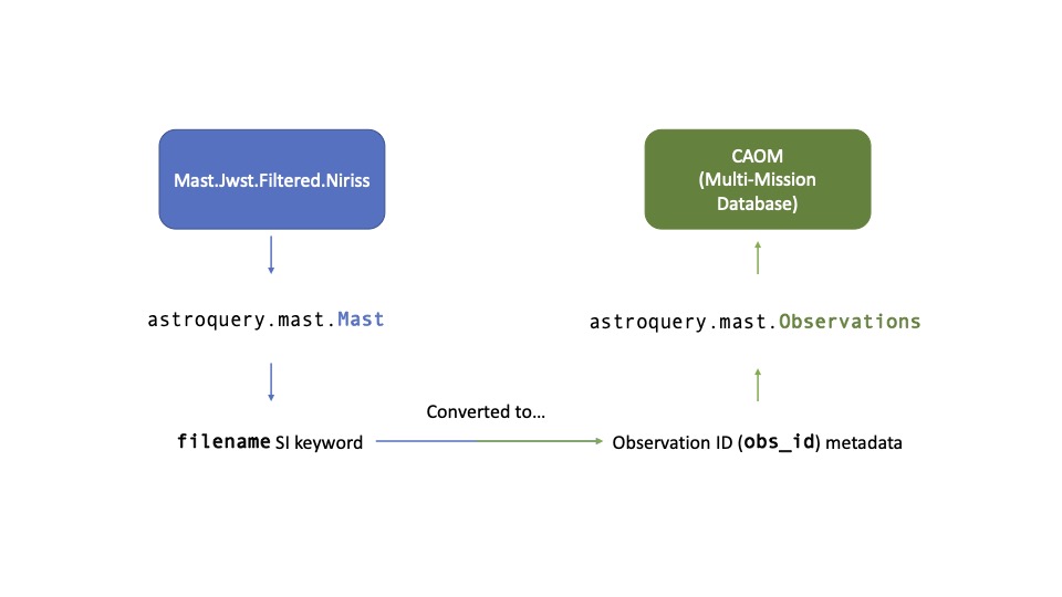
The keyword search returns an astropy table of files that match the query criteria. We need to construct MAST Observation IDs (obs_ids) from the file names in order to query for all JWST Observations that match our criteria. In a nutshell, we are deriving the obs_id from the files in one database (Mast.Jwst.Filtered.Niriss), to get the Observations from our multi-mission database (CAOM).
Construct the Observation Search#
The obs_id can be derived from the filenames by removing all characters after and including the final underscore character. Here we make a list of unique Observation IDs for the subsequent query. Note that we limit the list to unique IDs, as many filenames have common roots.
# Unique file names:
fn = list(set(t['filename']))

# Set of derived Observation IDs:
ids = list(set(['_'.join(x.split('_')[:-1]) for x in fn]))
Print the list of unique ids if you like.
ids
['jw01541001001_04101_00001-seg001_nis',
 'jw02734001001_04101_00001-seg002_nis',
 'jw01541001001_04101_00001-seg002_nis',
 'jw02734-o001_t001_niriss_clear-gr700xd-substrip256',
 'jw01091002001_03101_00001-seg003_nis',
 'jw01366001001_04101_00001-seg002_nis',
 'jw01091002001_03101_00001-seg002_nis',
 'jw01366001001_04101_00001-seg004_nis',
 'jw01091002001_03101_00001-seg005_nis',
 'jw02734002001_04102_00001-seg001_nis',
 'jw01541001001_04101_00001-seg003_nis',
 'jw02734001001_04101_00001-seg003_nis',
 'jw01091002001_03101_00001-seg004_nis',
 'jw02734001001_04101_00001-seg001_nis',
 'jw01366001001_04101_00001-seg001_nis',
 'jw01541-o001_t002_niriss_clear-gr700xd-substrip256',
 'jw01091002001_03102_00001-seg001_nis',
 'jw01541001001_04102_00001-seg001_nis',
 'jw01091-o002_t001_niriss_clear-gr700xd-substrip256',
 'jw02734002001_04101_00001-seg002_nis',
 'jw01366001001_04102_00001-seg001_nis',
 'jw01091002001_03101_00001-seg001_nis',
 'jw02734001001_04102_00001-seg001_nis',
 'jw01366001001_04101_00001-seg003_nis',
 'jw02734002001_04101_00001-seg001_nis',
 'jw02734002001_04101_00001-seg003_nis',
 'jw01541001001_04101_00001-seg004_nis',
 'jw01366-o001_t001_niriss_clear-gr700xd-substrip256',
 'jw02734001001_04101_00001-seg004_nis',
 'jw02734-o002_t002_niriss_clear-gr700xd-substrip256']
Execute the Query for Observations#
Now search for Observations that match the list of Observation IDs constructed above. This search uses the astroquery.mast Observations class, where the available search criteria are described here.
Note that the Observation ID (obs_id) criteria queried for here is not to be confused with the obsid that was shown in Crowded_Fields: The difference between the two criteria are explained in the CAOM Field Descriptions page linked just above.
# Getting the observations using the `obs_id`s extracted above
matched_obs = Observations.query_criteria(instrument_name='NIRISS*',
                                          obs_id=ids)

# Let's display the results
display_cols = [x for x in matched_obs.columns if x != 's_region']
matched_obs[display_cols]
| intentType | obs_collection | provenance_name | instrument_name | project | filters | wavelength_region | target_name | target_classification | obs_id | s_ra | s_dec | dataproduct_type | proposal_pi | calib_level | t_min | t_max | t_exptime | em_min | em_max | obs_title | t_obs_release | proposal_id | proposal_type | sequence_number | jpegURL | dataURL | dataRights | mtFlag | srcDen | obsid | objID |
|---|---|---|---|---|---|---|---|---|---|---|---|---|---|---|---|---|---|---|---|---|---|---|---|---|---|---|---|---|---|---|---|
| str7 | str4 | str7 | str11 | str4 | str13 | str8 | str10 | str54 | str50 | float64 | float64 | str10 | str21 | int64 | float64 | float64 | float64 | float64 | float64 | str70 | float64 | str4 | str3 | int64 | str80 | str81 | str6 | bool | float64 | str9 | str10 |
| science | JWST | CALJWST | NIRISS/SOSS | JWST | CLEAR;GR700XD | INFRARED | WASP-39 | Star; Exoplanet Systems | jw01366-o001_t001_niriss_clear-gr700xd-substrip256 | 217.32661044232407 | -3.444499322663515 | timeseries | Meech, Annabella | 3 | 59786.85676445602 | 59787.206306388885 | 26552.502 | 600.0 | 2800.0 | The Transiting Exoplanet Community Early Release Science Program | 59787.58458325 | 1366 | ERS | -- | mast:JWST/product/jw01366-o001_t001_niriss_clear-gr700xd-substrip256_x1dints.png | mast:JWST/product/jw01366-o001_t001_niriss_clear-gr700xd-substrip256_x1dints.fits | PUBLIC | False | nan | 87742481 | 997766155 |
| science | JWST | CALJWST | NIRISS/SOSS | JWST | CLEAR;GR700XD | INFRARED | WASP-39 | Star; Exoplanet Systems | jw01366001001_04102_00001-seg001_nis | 217.32661043978118 | -3.444499322617553 | timeseries | Meech, Annabella | 2 | 59787.207502997684 | 59787.21386416667 | 494.46 | 600.0 | 2800.0 | The Transiting Exoplanet Community Early Release Science Program | 59787.29994207 | 1366 | ERS | -- | mast:JWST/product/jw01366001001_04102_00001-seg001_nis_ramp.jpg | mast:JWST/product/jw01366001001_04102_00001-seg001_nis_rateints.fits | PUBLIC | False | nan | 87742159 | 998254698 |
| science | JWST | CALJWST | NIRISS/SOSS | JWST | CLEAR;GR700XD | INFRARED | WASP-96 | Star; Exoplanet Systems; Exoplanets; G dwarfs | jw02734-o002_t002_niriss_clear-gr700xd-substrip256 | 1.0466429207096102 | -47.36063076248256 | timeseries | Pontoppidan, Klaus M. | 3 | 59751.15883224537 | 59751.438179375 | 21536.48 | 600.0 | 2800.0 | JWST Early Release Observation 8 | 59773.625 | 2734 | COM | -- | mast:JWST/product/jw02734-o002_t002_niriss_clear-gr700xd-substrip256_x1dints.png | mast:JWST/product/jw02734-o002_t002_niriss_clear-gr700xd-substrip256_x1dints.fits | PUBLIC | False | nan | 118972907 | 1053143092 |
| science | JWST | CALJWST | NIRISS/SOSS | JWST | CLEAR;GR700XD | INFRARED | BD+60-1753 | Calibration; A stars; Photometric; Spectrophotometric | jw01091-o002_t001_niriss_clear-gr700xd-substrip256 | 261.2179184236822 | 60.43080397286861 | timeseries | Martel, Andre | 3 | 59735.26814030093 | 59735.498830358796 | 14438.232 | 600.0 | 2800.0 | NIRISS GR700XD Flux Calibration | 59774.8541666 | 1091 | COM | -- | mast:JWST/product/jw01091-o002_t001_niriss_clear-gr700xd-substrip256_x1dints.png | mast:JWST/product/jw01091-o002_t001_niriss_clear-gr700xd-substrip256_x1dints.fits | PUBLIC | False | nan | 118370229 | 1053732965 |
| science | JWST | CALJWST | NIRISS/SOSS | JWST | CLEAR;GR700XD | INFRARED | HAT-P-18 | Star; Exoplanet Systems; Exoplanets; K dwarfs | jw02734-o001_t001_niriss_clear-gr700xd-substrip256 | 256.3463434420834 | 33.01225418787759 | timeseries | Pontoppidan, Klaus M. | 3 | 59743.16453134259 | 59743.49048288194 | 23190.174 | 600.0 | 2800.0 | JWST Early Release Observation 8 | 60775.23592595 | 2734 | COM | -- | mast:JWST/product/jw02734-o001_t001_niriss_clear-gr700xd-substrip256_x1dints.png | mast:JWST/product/jw02734-o001_t001_niriss_clear-gr700xd-substrip256_x1dints.fits | PUBLIC | False | nan | 213209364 | 1056964668 |
| science | JWST | CALJWST | NIRISS/SOSS | JWST | CLEAR;GR700XD | INFRARED | HAT-P-14 | Star; Exoplanet Systems; Exoplanets; F dwarfs; F stars | jw01541-o001_t002_niriss_clear-gr700xd-substrip256 | 260.11617716308433 | 38.242156511096475 | timeseries | Espinoza, Nestor | 3 | 59738.26121493056 | 59738.552486493056 | 18855.408 | 600.0 | 2800.0 | NIRISS Sensitivity and Stability for Transiting Exoplanet Observations | 59774.8541666 | 1541 | COM | -- | mast:JWST/product/jw01541-o001_t002_niriss_clear-gr700xd-substrip256_x1dints.png | mast:JWST/product/jw01541-o001_t002_niriss_clear-gr700xd-substrip256_x1dints.fits | PUBLIC | False | nan | 213209384 | 1057262164 |
| science | JWST | CALJWST | NIRISS/SOSS | JWST | CLEAR;GR700XD | INFRARED | HAT-P-18 | Star; Exoplanet Systems; Exoplanets; K dwarfs | jw02734001001_04102_00001-seg001_nis | 256.3463434401183 | 33.012254183581504 | timeseries | Pontoppidan, Klaus M. | 2 | 59743.491782627316 | 59743.49877990741 | 543.906 | 600.0 | 2800.0 | JWST Early Release Observation 8 | 59773.625 | 2734 | COM | -- | mast:JWST/product/jw02734001001_04102_00001-seg001_nis_ramp.jpg | mast:JWST/product/jw02734001001_04102_00001-seg001_nis_rateints.fits | PUBLIC | False | nan | 87602090 | 1057446391 |
| science | JWST | CALJWST | NIRISS/SOSS | JWST | CLEAR;GR700XD | INFRARED | WASP-96 | Star; Exoplanet Systems; Exoplanets; G dwarfs | jw02734002001_04102_00001-seg001_nis | 1.0466429247344722 | -47.36063076224906 | timeseries | Pontoppidan, Klaus M. | 2 | 59751.43943215278 | 59751.44992677083 | 846.076 | 600.0 | 2800.0 | JWST Early Release Observation 8 | 59773.625 | 2734 | COM | -- | mast:JWST/product/jw02734002001_04102_00001-seg001_nis_ramp.jpg | mast:JWST/product/jw02734002001_04102_00001-seg001_nis_rateints.fits | PUBLIC | False | nan | 87599541 | 1057446423 |
| science | JWST | CALJWST | NIRISS/SOSS | JWST | CLEAR;GR700XD | INFRARED | BD+60-1753 | Calibration; A stars; Photometric; Spectrophotometric | jw01091002001_03102_00001-seg001_nis | 261.21791842457094 | 60.430803973205606 | timeseries | Martel, Andre | 2 | 59735.50011123843 | 59735.51029479167 | 659.28 | 600.0 | 2800.0 | NIRISS GR700XD Flux Calibration | 59774.8541666 | 1091 | COM | -- | mast:JWST/product/jw01091002001_03102_00001-seg001_nis_ramp.jpg | mast:JWST/product/jw01091002001_03102_00001-seg001_nis_rateints.fits | PUBLIC | False | nan | 84343071 | 1057717199 |
| science | JWST | CALJWST | NIRISS/SOSS | JWST | CLEAR;GR700XD | INFRARED | HAT-P-14 | Star; Exoplanet Systems; Exoplanets; F dwarfs; F stars | jw01541001001_04102_00001-seg001_nis | 260.1161771633686 | 38.24215651042749 | timeseries | Espinoza, Nestor | 2 | 59738.5539062963 | 59738.55835982639 | 329.64 | 600.0 | 2800.0 | NIRISS Sensitivity and Stability for Transiting Exoplanet Observations | 59774.8541666 | 1541 | COM | -- | mast:JWST/product/jw01541001001_04102_00001-seg001_nis_ramp.jpg | mast:JWST/product/jw01541001001_04102_00001-seg001_nis_rateints.fits | PUBLIC | False | nan | 85700205 | 1057802420 |
Verify that your query matched at least one observation, or the remaining steps will fail.
print(f'Found {len(matched_obs)} matching Observations.')
Found 10 matching Observations.
III: Download the Data Products#
Next we’ll download the data products that are connected to each Observation. In order to do this, we’ll need to query for our desired data products using the list of Observations we obtained above.
Query for Data Products#
Here we take care to fetch the products from Observations a few at a time (in batches) to avoid server timeouts. This can happen if there are a large number of files in one or more of the matched Observations. A larger batch size will execute faster, but increases the risk of a server timeout. A batch size of five offers is significantly faster than “one at a time”, while keeping the risk of timeout low.
The following bit of python magic splits one long list into a list of smaller lists, each of which has a size no larger than batch_size.
batch_size = 5
batches = [matched_obs[i:i+batch_size] for i in range(0, len(matched_obs), batch_size)]
Now fetch the constituent products in a list of tables.
t = [Observations.get_product_list(obs) for obs in batches]
We need to stack the individual tables and extract a unique set of file names. Observations often have many files in common (e.g., guide-star files) and this will avoid any duplicates.
products = unique(vstack(t), keys='productFilename')
print(f'  Number of unique products: {len(products)}')
Number of unique products: 564
Display the resulting list of files if you like.
products
| obsID | obs_collection | dataproduct_type | obs_id | description | type | dataURI | productType | productGroupDescription | productSubGroupDescription | productDocumentationURL | project | prvversion | proposal_id | productFilename | size | parent_obsid | dataRights | calib_level | filters |
|---|---|---|---|---|---|---|---|---|---|---|---|---|---|---|---|---|---|---|---|
| str9 | str4 | str10 | str50 | str64 | str1 | str81 | str9 | str28 | str13 | str1 | str7 | str6 | str4 | str63 | int64 | str9 | str6 | int64 | str13 |
| 84343195 | JWST | timeseries | jw01091002001_02101_00004-seg001_nis | source/target (L3) : association generator | S | mast:JWST/product/jw01091-o002_20251210t062745_image2_00001_asn.json | INFO | -- | ASN | -- | CALJWST | 1.10.1 | 1091 | jw01091-o002_20251210t062745_image2_00001_asn.json | 1437 | 118370229 | PUBLIC | 2 | CLEAR;GR700XD |
| 84343178 | JWST | timeseries | jw01091002001_02101_00003-seg001_nis | source/target (L3) : association generator | S | mast:JWST/product/jw01091-o002_20251210t062745_image2_00002_asn.json | INFO | -- | ASN | -- | CALJWST | 1.10.1 | 1091 | jw01091-o002_20251210t062745_image2_00002_asn.json | 1437 | 118370229 | PUBLIC | 2 | CLEAR;GR700XD |
| 84343036 | JWST | timeseries | jw01091002001_02101_00002-seg001_nis | source/target (L3) : association generator | S | mast:JWST/product/jw01091-o002_20251210t062745_image2_00003_asn.json | INFO | -- | ASN | -- | CALJWST | 1.10.1 | 1091 | jw01091-o002_20251210t062745_image2_00003_asn.json | 1437 | 118370229 | PUBLIC | 2 | CLEAR;GR700XD |
| 84343098 | JWST | timeseries | jw01091002001_02101_00001-seg001_nis | source/target (L3) : association generator | S | mast:JWST/product/jw01091-o002_20251210t062745_image2_00004_asn.json | INFO | -- | ASN | -- | CALJWST | 1.10.1 | 1091 | jw01091-o002_20251210t062745_image2_00004_asn.json | 1437 | 118370229 | PUBLIC | 2 | CLEAR;GR700XD |
| 84343158 | JWST | timeseries | jw01091002001_03101_00001-seg005_nis | source/target (L3) : association generator | S | mast:JWST/product/jw01091-o002_20251210t062745_tso-spec2_00001_asn.json | INFO | -- | ASN | -- | CALJWST | 1.20.2 | 1091 | jw01091-o002_20251210t062745_tso-spec2_00001_asn.json | 2090 | 118370229 | PUBLIC | 2 | CLEAR;GR700XD |
| 84343085 | JWST | timeseries | jw01091002001_03101_00001-seg004_nis | source/target (L3) : association generator | S | mast:JWST/product/jw01091-o002_20251210t062745_tso-spec2_00002_asn.json | INFO | -- | ASN | -- | CALJWST | 1.20.2 | 1091 | jw01091-o002_20251210t062745_tso-spec2_00002_asn.json | 2090 | 118370229 | PUBLIC | 2 | CLEAR;GR700XD |
| 84343207 | JWST | timeseries | jw01091002001_03101_00001-seg003_nis | source/target (L3) : association generator | S | mast:JWST/product/jw01091-o002_20251210t062745_tso-spec2_00003_asn.json | INFO | -- | ASN | -- | CALJWST | 1.20.2 | 1091 | jw01091-o002_20251210t062745_tso-spec2_00003_asn.json | 2090 | 118370229 | PUBLIC | 2 | CLEAR;GR700XD |
| 84343217 | JWST | timeseries | jw01091002001_03101_00001-seg002_nis | source/target (L3) : association generator | S | mast:JWST/product/jw01091-o002_20251210t062745_tso-spec2_00004_asn.json | INFO | -- | ASN | -- | CALJWST | 1.20.2 | 1091 | jw01091-o002_20251210t062745_tso-spec2_00004_asn.json | 2090 | 118370229 | PUBLIC | 2 | CLEAR;GR700XD |
| 84343025 | JWST | timeseries | jw01091002001_03101_00001-seg001_nis | source/target (L3) : association generator | S | mast:JWST/product/jw01091-o002_20251210t062745_tso-spec2_00005_asn.json | INFO | -- | ASN | -- | CALJWST | 1.20.2 | 1091 | jw01091-o002_20251210t062745_tso-spec2_00005_asn.json | 2090 | 118370229 | PUBLIC | 2 | CLEAR;GR700XD |
| ... | ... | ... | ... | ... | ... | ... | ... | ... | ... | ... | ... | ... | ... | ... | ... | ... | ... | ... | ... |
| 87599537 | JWST | timeseries | jw02734002001_04101_00001-seg003_nis | exposure/target (L2b/L3): 1D extracted spectrum per integration | S | mast:JWST/product/jw02734002001_04101_00001-seg003_nis_x1dints.fits | SCIENCE | -- | X1DINTS | -- | CALJWST | 1.20.2 | 2734 | jw02734002001_04101_00001-seg003_nis_x1dints.fits | 56361600 | 118972907 | PUBLIC | 2 | CLEAR;GR700XD |
| 87599541 | JWST | timeseries | jw02734002001_04102_00001-seg001_nis | exposure (L2a): corrected 4D data (up the ramp detection) | S | mast:JWST/product/jw02734002001_04102_00001-seg001_nis_ramp.fits | AUXILIARY | Minimum Recommended Products | RAMP | -- | CALJWST | 1.10.1 | 2734 | jw02734002001_04102_00001-seg001_nis_ramp.fits | 407975040 | 87599541 | PUBLIC | 2 | CLEAR;GR700XD |
| 87599541 | JWST | timeseries | jw02734002001_04102_00001-seg001_nis | Preview-Full | S | mast:JWST/product/jw02734002001_04102_00001-seg001_nis_ramp.jpg | PREVIEW | -- | -- | -- | CALJWST | 1.10.1 | 2734 | jw02734002001_04102_00001-seg001_nis_ramp.jpg | 55036 | 87599541 | PUBLIC | 2 | CLEAR;GR700XD |
| 87599541 | JWST | timeseries | jw02734002001_04102_00001-seg001_nis | exposure (L2a): 2D count rate averaged over integrations | S | mast:JWST/product/jw02734002001_04102_00001-seg001_nis_rate.fits | SCIENCE | Minimum Recommended Products | RATE | -- | CALJWST | 1.10.1 | 2734 | jw02734002001_04102_00001-seg001_nis_rate.fits | 10566720 | 87599541 | PUBLIC | 2 | CLEAR;GR700XD |
| 87599541 | JWST | timeseries | jw02734002001_04102_00001-seg001_nis | Preview-Full | S | mast:JWST/product/jw02734002001_04102_00001-seg001_nis_rate.jpg | PREVIEW | -- | -- | -- | CALJWST | 1.10.1 | 2734 | jw02734002001_04102_00001-seg001_nis_rate.jpg | 75102 | 87599541 | PUBLIC | 2 | CLEAR;GR700XD |
| 87599541 | JWST | timeseries | jw02734002001_04102_00001-seg001_nis | exposure (L2a): 3D countrate per integration | S | mast:JWST/product/jw02734002001_04102_00001-seg001_nis_rateints.fits | SCIENCE | Minimum Recommended Products | RATEINTS | -- | CALJWST | 1.10.1 | 2734 | jw02734002001_04102_00001-seg001_nis_rateints.fits | 115407360 | 87599541 | PUBLIC | 2 | CLEAR;GR700XD |
| 87599541 | JWST | timeseries | jw02734002001_04102_00001-seg001_nis | Preview-Full | S | mast:JWST/product/jw02734002001_04102_00001-seg001_nis_rateints.jpg | PREVIEW | -- | -- | -- | CALJWST | 1.10.1 | 2734 | jw02734002001_04102_00001-seg001_nis_rateints.jpg | 84936 | 87599541 | PUBLIC | 2 | CLEAR;GR700XD |
| 87599541 | JWST | timeseries | jw02734002001_04102_00001-seg001_nis | exposure (L1b): Uncalibrated 4D exposure data | S | mast:JWST/product/jw02734002001_04102_00001-seg001_nis_uncal.fits | SCIENCE | Minimum Recommended Products | UNCAL | -- | CALJWST | -- | 2734 | jw02734002001_04102_00001-seg001_nis_uncal.fits | 161530560 | 87599541 | PUBLIC | 1 | CLEAR;GR700XD |
| 87599541 | JWST | timeseries | jw02734002001_04102_00001-seg001_nis | Preview-Full | S | mast:JWST/product/jw02734002001_04102_00001-seg001_nis_uncal.jpg | PREVIEW | -- | -- | -- | CALJWST | -- | 2734 | jw02734002001_04102_00001-seg001_nis_uncal.jpg | 118569 | 87599541 | PUBLIC | 1 | CLEAR;GR700XD |
| 87599499 | JWST | timeseries | jw02734001001_02101_00004-seg001_nis | source/target (L3) : association pool | S | mast:JWST/product/jw02734_20251208t171330_pool.csv | INFO | -- | POOL | -- | CALJWST | 1.10.1 | 2734 | jw02734_20251208t171330_pool.csv | 8189 | 213209364 | PUBLIC | 2 | CLEAR;GR700XD |
Filter the Data Products#
If there are a subset of products of interest (or, a set of products you would like to exclude) there are a number of ways to do that. The cell below applies a filter to select only calibration level 2 and 3 spectral products classified as SCIENCE plus the INFO files that define product associations; it also excludes guide-star products. See the full set of Products Field Descriptions for the all queryable fields.
# Retrieve level 2 and 3 SCIENCE and INFO products of type spectrum.
filtered_products = Observations.filter_products(products,
                                                 productType=['SCIENCE', 'INFO'],
                                                 dataproduct_type='spectrum',
                                                 calib_level=[2, 3])
Display selected columns of the filtered products, if you like.
filtered_products['description', 'dataURI', 'calib_level', 'size', 'proposal_id']
| description | dataURI | calib_level | size | proposal_id |
|---|---|---|---|---|
| str64 | str81 | int64 | int64 | str4 |
Download the Data Products#
We’ll go over your options for data downloads in the sections below. Note that for public data, you will not need to login.
Optional: MAST Login#
If you intend to retrieve data that are protected by an Exclusive Access Period (EAP), you will need to be both authorized and authenticated. You can authenticate by presenting a valid Auth.MAST token with the login function. (See MAST User Accounts for more information about whether you need to login.)
This step is unnecessary if you are only retrieving public data.
- Create a token here: Auth.MAST
- Cut/paste the token string in response to the prompt that will appear when downloading the script.
# Observations.login()
Retrieve FIles#
Now let’s fetch the products. The example below shows how to retrieve a bash script (rather than direct file download) to retreive our entire list at once. Scripts are a much better choice if the number or size of files in the download manifest is large (more than 100 files or 10GB).
# Downloading via a bash script.

manifest = Observations.download_products(filtered_products,
                                          curl_flag=True)
WARNING: NoResultsWarning: No products to download. [astroquery.mast.observations]
In the interest of time (and not crashing our servers), we will download one small product from our list above. Let’s download a reasonably sized (~10MB) file. The file we choose is raw spectral data, so additional extraction would be needed for scientific analysis.
# We are fixing the file for reproducability
Observations.download_file("mast:JWST/product/jw02734001001_04101_00001-seg004_nis_rate.fits")
INFO: Found cached file jw02734001001_04101_00001-seg004_nis_rate.fits with expected size 10566720. [astroquery.query]
('COMPLETE', None, None)
Let’s actually visualize the raw data from which you can extract the spectrum:
# Read in the "SCI" data from the fits file
sci = fits.getdata("jw02734001001_04101_00001-seg004_nis_rate.fits", 1)

plt.figure(figsize=(15, 10))
plt.imshow(sci)
<matplotlib.image.AxesImage at 0x7f3a43f97310>
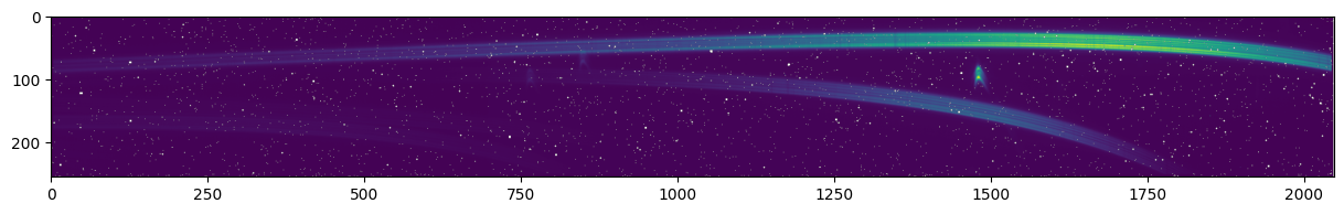
We are, in effect, seeing the cleaned spectrum on the detector; if you adjust the scaling you might be able to see the spectrum of order three in the lower left corner.
Additional Resources#
The links below take you to documentation that you might find useful when constructing queries.
astropy documentation
astroquery.mast documentation for querying MAST
Queryable fields in the MAST/CAOM database
About this notebook#
This notebook was developed by Archive Sciences Branch staff: chiefly Dick Shaw, with additional editing from Jenny Medina and Thomas Dutkiewicz.
For support, please contact the Archive HelpDesk at archive@stsci.edu, or through the JWST HelpDesk Portal.
Last updated: May 2023
