PySIAF Observation Footprint Viewer

PySIAF Observation Footprint Viewer#

Learning Goals#

Know the requirements for generating a telescope footprint
Create a plot of a footprint in the telescope’s reference frame
Create a plot of a footprint on the sky

Introduction#

This Notebook is a replacement for a web-based footprint viewer, and is designed as a “quick look” tool. Scientists intending to propose for Observations should use the Astronomer’s Proposal Tool (APT).

Note that since PySIAF only works for HST, JWST, and Roman, you cannot generate footprints for other telescopes using this notebook.

Imports#

ipyaladin plots the footprints on to a survey background
numpy is not listed in the import cell, but is necessary to run the selectSIAF script
selectSIAF is a script that uses SIAF to generate the telescope aperture names. Curious readers may wish to explore this file.
SIAF will translate the telescope pointing into corresponding sky footprints
time adds a pause to give Aladin time to load

from astropy.coordinates import SkyCoord
from ipyaladin import Aladin
from regions import Regions
from selectSIAF import defineApertures, getVertices, computeStcsFootprint, computeRegionFootprint
from getCatalog import gsss_stcsSearchUrl

import matplotlib.pyplot as plt
import os
import pysiaf
import time

Select a Telescope, Instrument, and Aperture#

In order to display a fooprint, we must first select three criteria:

Telescope. This must be a telescope with data in pysiaf; at present, this is HST, JWST, and Roman.
Instrument. The instrument used for the observation. The valid acronyms are listed in code comments in the cell below.
Aperture. For a full list of valid apertures, see the instrument documentation:
- HST User Documentation Homepage
- JWST MIRI Homepage (JWST has no instrument homepage; use the site navigation to reach other instrument pages)
- Roman Instruments Homepage

Example: Roman WFI#

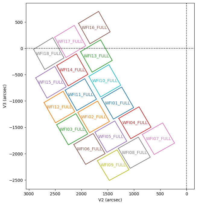
In the code cell below, we’ll set some variables to hold these three selections. In this example, we’re going to plot all 18 apertures from the Roman Space Telescope’s Wide Field Instrument.

For completeness, examples for HST and JWST are available but commented out.

# define telescope, instrument, and aperture

selectedTelescope = 'roman'
selectedInstrument = 'WFI'      # Allowed options ALL, WFI, CGI
selectedAperture = 'ALL'        # Allowed options ALL or individual apertures listed in instrument documentation

# selectedTelescope = 'hst'
# selectedInstrument = 'ALL'     # Allowed options ALL, ACS, COS, FGS, NICMOS, STIS, WFC3
# selectedAperture = 'ALL'       # Allowed options ALL or individual apertures listed in instrument documentation

# selectedTelescope = 'jwst'
# selectedInstrument = 'ALL'     # Allowed options ALL, FGS, MIRI, NIRCAM, NIRSPEC, NIRISS
# selectedAperture = 'ALL'       # Allowed options ALL or individual apertures listed in instrument documentation

Configure Apertures, Telescope Coordinate System#

To simplify this Notebook, the defineApertures function from selectSIAF is essentially a lookup table, translating user-friendly instrument names into the correct corresponding apertures.

This same function also generates the correct V2Ref and V3Ref offset angles. These V2/V3 values answer the question “what angles are there between this instrument and the line-of-sight of the telescope?”. This is quite useful since, barring a catastrophic event, the instruments do not change their alignment relative to the line-of-sight.

# Set up aperture list and reference coordinates
apertureList, V2Ref, V3Ref = defineApertures(selectedTelescope, selectedInstrument, selectedAperture)

Optional: Plot Footprint in Telescope Frame#

Although not necessary to generate the final image, it is possible to plot the telescope apertures. We’ll be plotting in a coordinate system that uses the telescope’s pointing direction as (0,0); because of this, we don’t need information about the celestial target or roll angle.

Note: labels are useful for Roman WFI, but may be cluttered for other missions. You can toggle them off by setting label=False below.

# OPTIONAL : set up plot of apertures (only works for QUAD, RECT, PICK aperture shapes)

# Set up the figure
plt.figure(figsize=(8, 8), facecolor='w', edgecolor='k')
plt.gca().invert_xaxis()

# iterate through apertures, then plot
for aperture in apertureList:
    # circles are not properly plotted, skip
    if aperture.AperShape != 'CIRC':
        # set labels=False to remove them
        aperture.plot(label=True)

# Add guide lines for boresight (V2, V3) = (0, 0)
plt.axvline(color='k', linestyle=":")
plt.axhline(color='k', linestyle=":")

# Display the plot
plt.show() 

../../../_images/dab3a2ca66f2cbd04819342c4a2d5dc90786b484095934b465ac69fc7e14080b.png

Specifying a Target#

For convenience, we can use the resolve_object function from the MAST module of astroquery to get our coordinates. This isn’t necessary if you already know the exact coordinates; however, you should note that the additional formatting steps below are necessary for PySIAF and Aladin to understand your query.

# Resolve the target name to coordinates
#coords = Mast.resolve_object("M101")
#coords

# Specify RA, Dec coordinates (This happens to be Arp 244)
coords = SkyCoord(180.46, -18.89, frame='icrs', unit='deg')

Using MAST to resolve our target returns a skycoord object. We need two different formats to satisfy pysiaf and Aladin. pysiaf requires separate ra/dec objects, while Aladin is looking for a string containing both.

Fortunately, skycoord objects are flexible enough to handle both of these requirements with straightforward calls:

# get the values for SIAF
targetRa = coords.ra
targetDec = coords.dec

coords_str = coords.to_string()

# print out these values to check their conversions
print(f"RA:     {targetRa}\nDEC:    {targetDec}\nString: {coords_str}")

RA:     180.46 deg
DEC:    -18.89 deg
String: 180.46 -18.89

There’s rounding in our RA/Dec as a result of our to_string() call. As we’ll see later on, we only need this string to point the Aladin viewer at the right section of the sky; a little bit of rounding won’t affect our view much.

Telescope Position Angle#

The last variable we need to set before using pysiaf is the telescope position angle. From the docstring of the attitude_matrix function:

Position angle of V3 axis at nu2,nu3 measured from North to East (default unit is degree)

In plain English, this is the telescope roll angle; with the telescope fixed on the target, it rotates around its V1 (line-of-sight) axis. Modifying this value will cause the footprints to “roll” around the target.

# can be any value between 0 and 360
telescopePositionAngle = 0

Generate The Attitude Matrix#

At this point, we’ve generated footprints in the telescope’s field of view. Now, we need to translate this into a view on the sky, in RA/Dec coordinates. This is handled by the attitude_matrix function, which is doing some matrix multiplication behind the scenes.

# Set telescope pointing matrix: "attitude matrix"
attmat = pysiaf.utils.rotations.attitude_matrix(V2Ref, V3Ref, targetRa, targetDec, telescopePositionAngle)

Calculate Sky Regions#

The final step is to convert to the IVOA Space-Time Coordinate Metadata Linear String Implementation (STS-C). Do not fear this verbose name; it’s a method of standardizing footprints in string formats. The specifics depend on the particular shape used. For the curious, the computeStcsFootprint function from selectSIAF is what calcuates these strings in this Notebook.

Since Aladin knows how to parse this format, it will be able to plot it on a sky background of our choice. It is not particularly human readable, but we’ll print it out anyway.

# Loop through aperture list  (only works for QUAD, RECT, CIRC aperture shapes)
# Transform to sky coordinates, build footprints for passing to Aladin
combinedSregion = ''
for apertureSiaf in apertureList:
    apertureSiaf.set_attitude_matrix(attmat)
    xVertices, yVertices = getVertices(apertureSiaf)
    
    # Skip PICK which do not have vertices (HST/FGS is only instrument affected)
    if (xVertices is not None and yVertices is not None):
        skyRa, skyDec = apertureSiaf.idl_to_sky(xVertices, yVertices)
        apertureSregion = computeStcsFootprint(apertureSiaf, skyRa, skyDec)
        combinedSregion += apertureSregion
        
print('\n'+combinedSregion)

POLYGON ICRS 180.48076550 -18.90746286 180.36817811 -18.84599471 180.30142864 -18.95458865 180.41432099 -19.01546832 POLYGON ICRS 180.61337499 -18.98023404 180.50312512 -18.92019002 180.43676136 -19.02805554 180.54742848 -19.08735321 POLYGON ICRS 180.73180882 -19.04512674 180.62417451 -18.98663388 180.55826413 -19.09366679 180.66641297 -19.15127114 POLYGON ICRS 180.38476223 -19.01148376 180.27151502 -18.95039598 180.20444240 -19.05820395 180.31779889 -19.11865545 POLYGON ICRS 180.51784519 -19.08456614 180.40670457 -19.02503169 180.33977788 -19.13204690 180.45115278 -19.19078688 POLYGON ICRS 180.63621633 -19.14933193 180.52749585 -19.09145779 180.46082317 -19.19758215 180.56989072 -19.25453642 POLYGON ICRS 180.25335389 -19.09618812 180.13933659 -19.03514272 180.07241672 -19.14183101 180.18632000 -19.20224512 POLYGON ICRS 180.38735634 -19.16989687 180.27504199 -19.11044795 180.20799062 -19.21633154 180.32031836 -19.27498977 POLYGON ICRS 180.50441635 -19.23522897 180.39414431 -19.17747224 180.32711227 -19.28245617 180.43751048 -19.33930232 POLYGON ICRS 180.55186501 -18.79003011 180.43978571 -18.72802620 180.37369416 -18.83696491 180.48624657 -18.89847599 POLYGON ICRS 180.68422620 -18.86286330 180.57459440 -18.80208536 180.50908867 -18.91041251 180.61929164 -18.97052512 POLYGON ICRS 180.80236003 -18.92794523 180.69543451 -18.86855323 180.63056183 -18.97614645 180.73814330 -19.03472259 POLYGON ICRS 180.59805274 -18.65938855 180.48626383 -18.59681364 180.42103650 -18.70560914 180.53344622 -18.76782628 POLYGON ICRS 180.73061197 -18.73228130 180.62127088 -18.67067106 180.55680842 -18.77901247 180.66685926 -18.84007709 POLYGON ICRS 180.84833093 -18.79722860 180.74166672 -18.73677286 180.67800074 -18.84451218 180.78542545 -18.90427161 POLYGON ICRS 180.60897167 -18.50998880 180.49711324 -18.44690783 180.43278142 -18.55497840 180.54537773 -18.61789326 POLYGON ICRS 180.74222983 -18.58314454 180.63263703 -18.52068177 180.56922676 -18.62850933 180.67962961 -18.69061808 POLYGON ICRS 180.85952385 -18.64657059 180.75243600 -18.58495039 180.68994762 -18.69236940 180.79789349 -18.75348418 

Optional: Create DS9 region file with footprints#

Although not necessary to generate the final image, it is possible to write the footprints to a DS9 region file. Here, we’ll create a file called regionTest.reg.

# OPTIONAL build same footprints for creating a DS9 region file

regionList = []
for i in range(len(apertureList)):
    apertureSiaf = apertureList[i]
    apertureSiaf.set_attitude_matrix(attmat)
    xVertices, yVertices = getVertices(apertureSiaf)
    
    # Skip PICK which do not have vertices
    if (xVertices is not None and yVertices is not None):
        skyRa, skyDec = apertureSiaf.idl_to_sky(xVertices, yVertices)
        apertureRegion = computeRegionFootprint(apertureSiaf, skyRa, skyDec)
        regionList.append(apertureRegion)
        
# Provide a writeable file location on your system
regionFile = 'regionTest.reg'
if os.path.isfile(regionFile):
    os.remove(regionFile)
combinedRegion = Regions(regionList)
combinedRegion.write(regionFile)

Initialize Aladin#

Let’s start the Aladin viewer. We’re loading a default field of view of 1 degree, with DSS as the background survey. Depending on your screen size, you may need to adjust the height (in pixels) to get the best view.

NOTE: The footprint will not be displayed in the rendered HTML. Please download and run it locally, or use TIKE.

aladin = Aladin(height=600, fov=1, survey="P/DSS2/color", target=coords_str)
aladin

# Pause for 2 seconds to give Aladin time to load the viewer
# Necessary when using "Run All Cells", or even just hitting 'shift+enter' fast enough
time.sleep(2)

# Add the footprint with a hexcode for the color; you can also enter, e.g. "green"
aladin.add_overlay_from_stcs(combinedSregion, color="#70CBFF")

/tmp/ipykernel_1850/3484408755.py:6: DeprecationWarning: 'add_overlay_from_stcs' is deprecated, use 'add_graphic_overlay_from_stcs' instead
  aladin.add_overlay_from_stcs(combinedSregion, color="#70CBFF")

Done! Err… well, almost done. Aladin will only show the footprint when you mouse over the display or make another change to it.

Let’s change the display size from the command line to force the footprint to appear.

aladin.fov = 2

Done! The footprint is now visible in the Aladin window.

Add a Catalog#

You can also overlay catalog sources onto the viewer. Clicking on these sources will show their names, RA/decs, and any other information included in the catalog.

# Optional Retrieve catalog sources from MAST that are within footprint and overlay them
# Supported catalogs : 'GSC11', 'GSC243', 'GSC30', '2MASS', 'GAIADR3'  

#selectedCatalog = 'GSC11'
#selectedCatalog = 'GSC243'
#selectedCatalog = 'GSC30'
#selectedCatalog = '2MASS'
selectedCatalog = 'GAIADR3'

url = gsss_stcsSearchUrl(combinedSregion,  catalog=selectedCatalog)
options = {'source_size': 12, 'onClick': 'showTable', 'name': selectedCatalog}
aladin.add_catalog_from_URL(url, options)

About this Notebook#

If you have comments or questions on this notebook, please contact us through the Archive Help Desk e-mail at archive@stsci.edu.

Authors: Brian McLean, Thomas Dutkiewicz
Keywords: Footprints
Last Updated: June 2024

Top of Page