Plotting a Catalog over a Kepler Full Frame Image File

This tutorial demonstrates how to access the WCS (World Coordinate System) from a full frame image file and use this data to plot a catalog of objects over the FFI.

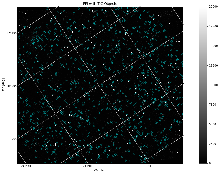
Table of Contents

Introduction
Imports
Getting the Data
File Information
Displaying Image Data
Overplotting Objects
Additional Resources
About this Notebook

---

Introduction

Full Frame Image file background: A Full Frame Image (FFI) contains values for every pixel in each of the 84 channels. Standard calibrations, such as flat fields, blacks, and smears have been applied to the calibrated FFIs. These files also contain a World Coordinate System (WCS) that attaches RA and Dec coordinates to pixel x and y values.

Some notes about the file: kplr2009170043915_ffi-cal.fits
The filename contains phrases for identification, where

• kplr = Kepler

• 2009170043915 = year 2009, day 170, time 04:39:15

• ffi-cal = calibrated FFI image

Defining some terms:

• HDU: Header Data Unit; a FITS file is made up of Header or Data units that contain information, data, and metadata relating to the file. The first HDU is called the primary, and anything that follows is considered an extension.

• TIC: TESS Input Catalog; a catalog of luminous sources on the sky to be used by the TESS mission. We will use the TIC in this notebook to query a catalog of objects that we will then plot over an image from Kepler.

• WCS: World Coordinate System; coordinates attached to each pixel of an N-dimensional image of a FITS file. For example, a specified celestial RA and Dec associated with pixel location in the image.

For more information about the Kepler mission and collected data, visit the Kepler archive page. To read more details about light curves and important data terms, look in the Kepler archive manual.

Top of Page

---

Imports

Let’s start by importing some libraries to the environment:

• numpy to handle array functions

• astropy.io fits for accessing fits files

• astropy.wcs WCS to project the World Coordinate System on the plot

• astropy.table Table for creating tidy tables of the data

• matplotlib.pyplot for plotting data

%matplotlib inline
import numpy as np
from astropy.io import fits
from astropy.wcs import WCS
from astropy.table import Table
import matplotlib.pyplot as plt

Top of Page

---

Getting the Data

Start by importing libraries from Astroquery. For a longer, more detailed description using of Astroquery, please visit this tutorial or read the Astroquery documentation.

from astroquery.mast import Mast
from astroquery.mast import Observations

Next, we need to find the data file. This is similar to searching for the data using the MAST Portal in that we will be using certain keywords to find the file. The object we are looking for is kplr2009170043915, collected by the Kepler spacecraft. We are searching for an FFI file of this object:

kplrObs = Observations.query_criteria(obs_id="kplr2009170043915_84", obs_collection="KeplerFFI")
kplrProds = Observations.get_product_list(kplrObs[0])
yourProd = Observations.filter_products(kplrProds, extension='kplr2009170043915_ffi-cal.fits', 
                                        mrp_only=False)
yourProd

Table masked=True length=1

obsID	obs_collection	dataproduct_type	obs_id	description	type	dataURI	productType	productGroupDescription	productSubGroupDescription	productDocumentationURL	project	prvversion	proposal_id	productFilename	size	parent_obsid	dataRights	calib_level	filters
str6	str9	str5	str20	str22	str1	str106	str7	str28	str1	str1	str6	str1	str1	str37	int64	str6	str6	int64	str6
385623	KeplerFFI	image	kplr2009170043915_84	Full Frame Image (FFI)	C	mast:KEPLERFFI/url/missions/kepler/ffi/kplr2009170043915_ffi-cal.fits	SCIENCE	Minimum Recommended Products	--	--	Kepler	--	--	kplr2009170043915_ffi-cal.fits	407882880	385623	PUBLIC	1	KEPLER

Now that we’ve found the data file, we can download it using the reults shown in the table above:

Observations.download_products(yourProd, mrp_only=False, cache=False)

Downloading URL https://mast.stsci.edu/api/v0.1/Download/file?uri=mast:KEPLERFFI/url/missions/kepler/ffi/kplr2009170043915_ffi-cal.fits to ./mastDownload/KeplerFFI/kplr2009170043915_84/kplr2009170043915_ffi-cal.fits ...

 [Done]

Table length=1

Local Path	Status	Message	URL
str76	str8	object	object
./mastDownload/KeplerFFI/kplr2009170043915_84/kplr2009170043915_ffi-cal.fits	COMPLETE	None	None

Top of Page

---

Reading FITS Extensions

Now that we have the file, we can start working with the data. We will begin by assigning a shorter name to the file to make it easier to use. Then, using the info function from astropy.io.fits, we can see some information about the FITS Header Data Units:

filename = "./mastDownload/KeplerFFI/kplr2009170043915_84/kplr2009170043915_ffi-cal.fits"
fits.info(filename)

Filename: ./mastDownload/KeplerFFI/kplr2009170043915_84/kplr2009170043915_ffi-cal.fits
No.    Name      Ver    Type      Cards   Dimensions   Format
  0  PRIMARY       1 PrimaryHDU      57   ()      
  1  MOD.OUT 2.1    1 ImageHDU       100   (1132, 1070)   float32   
  2  MOD.OUT 2.2    1 ImageHDU       100   (1132, 1070)   float32   
  3  MOD.OUT 2.3    1 ImageHDU       100   (1132, 1070)   float32   
  4  MOD.OUT 2.4    1 ImageHDU       100   (1132, 1070)   float32   
  5  MOD.OUT 3.1    1 ImageHDU       100   (1132, 1070)   float32   
  6  MOD.OUT 3.2    1 ImageHDU       100   (1132, 1070)   float32   
  7  MOD.OUT 3.3    1 ImageHDU       100   (1132, 1070)   float32   
  8  MOD.OUT 3.4    1 ImageHDU       100   (1132, 1070)   float32   
  9  MOD.OUT 4.1    1 ImageHDU       100   (1132, 1070)   float32   
 10  MOD.OUT 4.2    1 ImageHDU       100   (1132, 1070)   float32   
 11  MOD.OUT 4.3    1 ImageHDU       100   (1132, 1070)   float32   
 12  MOD.OUT 4.4    1 ImageHDU       100   (1132, 1070)   float32   
 13  MOD.OUT 6.1    1 ImageHDU       100   (1132, 1070)   float32   
 14  MOD.OUT 6.2    1 ImageHDU       100   (1132, 1070)   float32   
 15  MOD.OUT 6.3    1 ImageHDU       100   (1132, 1070)   float32   
 16  MOD.OUT 6.4    1 ImageHDU       100   (1132, 1070)   float32   
 17  MOD.OUT 7.1    1 ImageHDU       100   (1132, 1070)   float32   
 18  MOD.OUT 7.2    1 ImageHDU       100   (1132, 1070)   float32   
 19  MOD.OUT 7.3    1 ImageHDU       100   (1132, 1070)   float32   
 20  MOD.OUT 7.4    1 ImageHDU       100   (1132, 1070)   float32   
 21  MOD.OUT 8.1    1 ImageHDU       100   (1132, 1070)   float32   
 22  MOD.OUT 8.2    1 ImageHDU       100   (1132, 1070)   float32   
 23  MOD.OUT 8.3    1 ImageHDU       100   (1132, 1070)   float32   
 24  MOD.OUT 8.4    1 ImageHDU       100   (1132, 1070)   float32   
 25  MOD.OUT 9.1    1 ImageHDU       100   (1132, 1070)   float32   
 26  MOD.OUT 9.2    1 ImageHDU       100   (1132, 1070)   float32   
 27  MOD.OUT 9.3    1 ImageHDU       100   (1132, 1070)   float32   
 28  MOD.OUT 9.4    1 ImageHDU       100   (1132, 1070)   float32   
 29  MOD.OUT 10.1    1 ImageHDU       100   (1132, 1070)   float32   
 30  MOD.OUT 10.2    1 ImageHDU       100   (1132, 1070)   float32   
 31  MOD.OUT 10.3    1 ImageHDU       100   (1132, 1070)   float32   
 32  MOD.OUT 10.4    1 ImageHDU       100   (1132, 1070)   float32   
 33  MOD.OUT 11.1    1 ImageHDU       100   (1132, 1070)   float32   
 34  MOD.OUT 11.2    1 ImageHDU       100   (1132, 1070)   float32   
 35  MOD.OUT 11.3    1 ImageHDU       100   (1132, 1070)   float32   
 36  MOD.OUT 11.4    1 ImageHDU       100   (1132, 1070)   float32   
 37  MOD.OUT 12.1    1 ImageHDU       100   (1132, 1070)   float32   
 38  MOD.OUT 12.2    1 ImageHDU       100   (1132, 1070)   float32   
 39  MOD.OUT 12.3    1 ImageHDU       100   (1132, 1070)   float32   
 40  MOD.OUT 12.4    1 ImageHDU       100   (1132, 1070)   float32   
 41  MOD.OUT 13.1    1 ImageHDU       100   (1132, 1070)   float32   
 42  MOD.OUT 13.2    1 ImageHDU       100   (1132, 1070)   float32   
 43  MOD.OUT 13.3    1 ImageHDU       100   (1132, 1070)   float32   
 44  MOD.OUT 13.4    1 ImageHDU       100   (1132, 1070)   float32   
 45  MOD.OUT 14.1    1 ImageHDU       100   (1132, 1070)   float32   
 46  MOD.OUT 14.2    1 ImageHDU       100   (1132, 1070)   float32   
 47  MOD.OUT 14.3    1 ImageHDU       100   (1132, 1070)   float32   
 48  MOD.OUT 14.4    1 ImageHDU       100   (1132, 1070)   float32   
 49  MOD.OUT 15.1    1 ImageHDU       100   (1132, 1070)   float32   
 50  MOD.OUT 15.2    1 ImageHDU       100   (1132, 1070)   float32   
 51  MOD.OUT 15.3    1 ImageHDU       100   (1132, 1070)   float32   
 52  MOD.OUT 15.4    1 ImageHDU       100   (1132, 1070)   float32   
 53  MOD.OUT 16.1    1 ImageHDU       100   (1132, 1070)   float32   
 54  MOD.OUT 16.2    1 ImageHDU       100   (1132, 1070)   float32   
 55  MOD.OUT 16.3    1 ImageHDU       100   (1132, 1070)   float32   
 56  MOD.OUT 16.4    1 ImageHDU       100   (1132, 1070)   float32   
 57  MOD.OUT 17.1    1 ImageHDU       100   (1132, 1070)   float32   
 58  MOD.OUT 17.2    1 ImageHDU       100   (1132, 1070)   float32   
 59  MOD.OUT 17.3    1 ImageHDU       100   (1132, 1070)   float32   
 60  MOD.OUT 17.4    1 ImageHDU       100   (1132, 1070)   float32   
 61  MOD.OUT 18.1    1 ImageHDU       100   (1132, 1070)   float32   
 62  MOD.OUT 18.2    1 ImageHDU       100   (1132, 1070)   float32   
 63  MOD.OUT 18.3    1 ImageHDU       100   (1132, 1070)   float32   
 64  MOD.OUT 18.4    1 ImageHDU       100   (1132, 1070)   float32   
 65  MOD.OUT 19.1    1 ImageHDU       100   (1132, 1070)   float32   
 66  MOD.OUT 19.2    1 ImageHDU       100   (1132, 1070)   float32   
 67  MOD.OUT 19.3    1 ImageHDU       100   (1132, 1070)   float32   
 68  MOD.OUT 19.4    1 ImageHDU       100   (1132, 1070)   float32   
 69  MOD.OUT 20.1    1 ImageHDU       100   (1132, 1070)   float32   
 70  MOD.OUT 20.2    1 ImageHDU       100   (1132, 1070)   float32   
 71  MOD.OUT 20.3    1 ImageHDU       100   (1132, 1070)   float32   
 72  MOD.OUT 20.4    1 ImageHDU       100   (1132, 1070)   float32   
 73  MOD.OUT 22.1    1 ImageHDU       100   (1132, 1070)   float32   
 74  MOD.OUT 22.2    1 ImageHDU       100   (1132, 1070)   float32   
 75  MOD.OUT 22.3    1 ImageHDU       100   (1132, 1070)   float32   
 76  MOD.OUT 22.4    1 ImageHDU       100   (1132, 1070)   float32   
 77  MOD.OUT 23.1    1 ImageHDU       100   (1132, 1070)   float32   
 78  MOD.OUT 23.2    1 ImageHDU       100   (1132, 1070)   float32   
 79  MOD.OUT 23.3    1 ImageHDU       100   (1132, 1070)   float32   
 80  MOD.OUT 23.4    1 ImageHDU       100   (1132, 1070)   float32   
 81  MOD.OUT 24.1    1 ImageHDU       100   (1132, 1070)   float32   
 82  MOD.OUT 24.2    1 ImageHDU       100   (1132, 1070)   float32   
 83  MOD.OUT 24.3    1 ImageHDU       100   (1132, 1070)   float32   
 84  MOD.OUT 24.4    1 ImageHDU       100   (1132, 1070)   float32   

• **No. 0 (Primary): **
  This HDU contains meta-data related to the entire file.

• **No. 1-84 (Image): **
  Each of the 84 image extensions contains an array that can be plotted as an image. We will plot one in this tutorial along with catalog data.

Let’s say we wanted to see more information about the header and extensions than what the fits.info command gave us. For example, we can access information stored in the header of any of the Image extensions (No.1 - 84, MOD.OUT). The following line opens the FITS file, writes the first HDU extension into header1, and then closes the file. Only 24 rows of data are displayed here but you can view them all by adjusting the range:

with fits.open(filename) as hdulist: 
    header1 = hdulist[1].header
  
print(repr(header1[1:25]))

BITPIX  =                  -32 / array data type                                
NAXIS   =                    2 / NAXIS                                          
NAXIS1  =                 1132 / length of first array dimension                
NAXIS2  =                 1070 / length of second array dimension               
PCOUNT  =                    0 / group parameter count (not used)               
GCOUNT  =                    1 / group count (not used)                         
INHERIT =                    T / inherit the primary header                     
EXTNAME = 'MOD.OUT 2.1'        / name of extension                              
EXTVER  =                    1 / extension version number (not format version)  
TELESCOP= 'Kepler  '           / telescope                                      
INSTRUME= 'Kepler Photometer'  / detector type                                  
CHANNEL =                    1 / CCD channel                                    
SKYGROUP=                   81 / roll-independent location of channel           
MODULE  =                    2 / CCD module                                     
OUTPUT  =                    1 / CCD output                                     
TIMEREF = 'SOLARSYSTEM'        / barycentric correction applied to times        
TASSIGN = 'SPACECRAFT'         / where time is assigned                         
TIMESYS = 'TDB     '           / time system is barycentric JD                  
MJDSTART=       55001.17349214 / [d] start of observation in spacecraft MJD     
MJDEND  =        55001.1939257 / [d] end of observation in spacecraft MJD       
BJDREFI =              2454833 / integer part of BJD reference date             
BJDREFF =           0.00000000 / fraction of the day in BJD reference date      
TIMEUNIT= 'd       '           / time unit for TIME, TSTART and TSTOP           
TSTART  =         168.67667104 / observation start time in BJD-BJDREF           

Top of Page

---

Displaying Image Data

First, let’s find the WCS information associated with the FITS file we are using. One way to do this is to access the header and print the rows containing the relevant data (54 - 65). This gives us the reference coordinates (CRVAL1, CRVAL2) that correspond to the reference pixels:

with fits.open(filename) as hdulist: 
    header1 = hdulist[1].header
  
print(repr(header1[54:61]))

WCSAXES =                    2 / number of WCS axes                             
CTYPE1  = 'RA---TAN-SIP'       / Gnomonic projection + SIP distortions          
CTYPE2  = 'DEC--TAN-SIP'       / Gnomonic projection + SIP distortions          
CRVAL1  =    290.4620065226813 / RA at CRPIX1, CRPIX2                           
CRVAL2  =    38.32946356799192 / DEC at CRPIX1, CRPIX2                          
CRPIX1  =                533.0 / X reference pixel                              
CRPIX2  =                521.0 / Y reference pixel                              

Let’s pick an image HDU and display its array. We can also choose to print the length of the array to get an idea of the dimensions of the image:

with fits.open(filename) as hdulist:
    imgdata = hdulist[1].data
    
print(len(imgdata))
print(imgdata)

1070
[[ 2.8926212e+01  5.7084761e+00  2.8518679e+00 ...  2.3335369e-02
   3.8872162e-01  2.4866710e+00]
 [ 2.5392172e+01  4.9826989e+00  2.3192320e+00 ... -3.5835370e-01
   9.4126135e-01  1.4343496e-01]
 [ 2.7359493e+01  5.5186005e+00  1.1480473e+00 ...  5.8914202e-01
  -2.0753877e+00  2.3046710e-01]
 ...
 [-3.8266034e+02 -9.6860485e+00  1.7396482e+01 ...  1.3947951e+00
  -8.3887035e-01  9.5944041e-01]
 [-3.8286859e+02 -5.6933088e+00  2.0129442e+01 ... -7.7534288e-01
   1.5140564e+00  1.3752979e+00]
 [-3.8489960e+02 -3.4747849e+00  1.5189555e+00 ...  1.0207459e+00
   6.7454106e-01 -2.0665376e-02]]

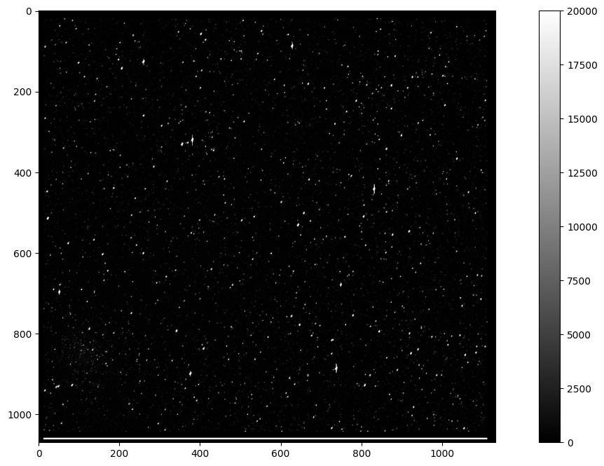
We can now plot this array as an image:

fig = plt.figure(figsize=(16,8))
plt.imshow(imgdata, cmap=plt.cm.gray)
plt.colorbar()
plt.clim(0,20000)

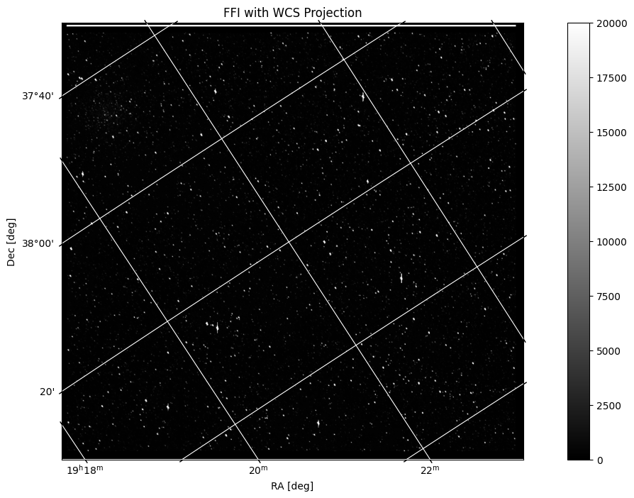
Now that we’ve seen the image and the WCS information, we can plot FFI with a WCS projection. To do this, first we will access the file header and assign a WCS object. Then we will plot the image with the projection, and add labels and a grid for usability:

hdu = fits.open(filename)[1]
wcs = WCS(hdu.header)

fig = plt.figure(figsize=(16,8))
ax = plt.subplot(projection=wcs) 
im = ax.imshow(hdu.data, cmap=plt.cm.gray, origin='lower', clim=(0,20000))
fig.colorbar(im)

plt.title('FFI with WCS Projection')
ax.set_xlabel('RA [deg]')
ax.set_ylabel('Dec [deg]')
ax.grid(color='white', ls='solid')

WARNING: FITSFixedWarning: 'datfix' made the change 'Set MJD-OBS to 55001.173492 from DATE-OBS.
Set MJD-END to 55001.193926 from DATE-END'. [astropy.wcs.wcs]

Top of Page

---

Getting the Catalog Data

Now that we have an image, we can use astroquery to retrieve a catalog of objects and overlay it onto the image. First, we will start with importing catalog data from astroquery:

from astroquery.mast import Catalogs

We will query a catalog of objects from TIC (TESS Input Catalog). For more information about TIC, follow this link. Our search will be centered on the same RA and Declination listed in the header of the FFI image and will list objects within a 1 degree radius of that location. It might take a couple seconds longer than usual for this cell to run:

why tic??? explain…

catalogData = Catalogs.query_region("290.4620065226813  38.32946356799192", radius="0.2 deg", catalog="TIC")
dattab = Table(catalogData)
dattab

WARNING: InputWarning: Coordinate string is being interpreted as an ICRS coordinate provided in degrees. [astroquery.utils.commons]

Table length=7955

ID	ra	dec	pmRA	pmDEC	Tmag	objType	typeSrc	version	HIP	TYC	UCAC	TWOMASS	SDSS	ALLWISE	GAIA	APASS	KIC	POSflag	e_pmRA	e_pmDEC	PMflag	plx	e_plx	PARflag	gallong	gallat	eclong	eclat	Bmag	e_Bmag	Vmag	e_Vmag	umag	e_umag	gmag	e_gmag	rmag	e_rmag	imag	e_imag	zmag	e_zmag	Jmag	e_Jmag	Hmag	e_Hmag	Kmag	e_Kmag	TWOMflag	prox	w1mag	e_w1mag	w2mag	e_w2mag	w3mag	e_w3mag	w4mag	e_w4mag	GAIAmag	e_GAIAmag	e_Tmag	TESSflag	SPFlag	Teff	e_Teff	logg	e_logg	MH	e_MH	rad	e_rad	mass	e_mass	rho	e_rho	lumclass	lum	e_lum	d	e_d	ebv	e_ebv	numcont	contratio	disposition	duplicate_id	priority	eneg_EBV	epos_EBV	EBVflag	eneg_Mass	epos_Mass	eneg_Rad	epos_Rad	eneg_rho	epos_rho	eneg_logg	epos_logg	eneg_lum	epos_lum	eneg_dist	epos_dist	distflag	eneg_Teff	epos_Teff	TeffFlag	gaiabp	e_gaiabp	gaiarp	e_gaiarp	gaiaqflag	starchareFlag	VmagFlag	BmagFlag	splists	e_RA	e_Dec	RA_orig	Dec_orig	e_RA_orig	e_Dec_orig	raddflag	wdflag	dstArcSec
str11	float64	float64	float64	float64	float64	str8	str7	str8	str1	str12	str10	str16	str19	str19	str19	str8	str7	str8	float64	float64	str6	float64	float64	str5	float64	float64	float64	float64	float64	float64	float64	float64	float64	float64	float64	float64	float64	float64	float64	float64	float64	float64	float64	float64	float64	float64	float64	float64	str19	float64	float64	float64	float64	float64	float64	float64	float64	float64	float64	float64	float64	str5	str5	float64	float64	float64	float64	float64	float64	float64	float64	float64	float64	float64	float64	str5	float64	float64	float64	float64	float64	float64	int64	float64	str9	str11	float64	float64	float64	str9	float64	float64	float64	float64	float64	float64	float64	float64	float64	float64	float64	float64	str6	float64	float64	str5	float64	float64	float64	float64	int64	str1	str8	str8	str13	float64	float64	float64	float64	float64	float64	int64	int64	float64
1877313283	290.460664282612	38.3304513142701	-5.59848	-4.23894	19.8414	STAR	gaia2	20190415	--	--	--	--	1237668681001865025	--	2052812123437410304	--	--	gaia2	1.44352	1.32282	gaia2	1.03985	0.761685	gaia2	70.5543455582815	10.9790727152229	302.670882604946	59.4705457723064	nan	nan	20.8787	0.0823	30.0	50.0	21.7964	0.0646979	20.5154	0.0313574	20.0153	0.0339539	19.6638	0.0813132	nan	nan	nan	nan	nan	nan	--	nan	nan	nan	nan	nan	nan	nan	nan	nan	20.525	0.008983	0.0199	gbprp	gaia2	nan	nan	nan	nan	nan	nan	nan	nan	nan	nan	nan	nan	--	nan	nan	1841.43	1612.4	0.100619	0.0172583	--	nan	--	--	nan	0.0227474	0.0117692	panstarrs	nan	nan	nan	nan	nan	nan	nan	nan	nan	nan	1032.03	2192.77	bj2018	nan	nan	--	21.0082	0.117128	19.6349	0.077334	0	--	gaia2	--	--	23.696890381893	20.5150830759397	290.460633554505	38.3304330632823	0.663291984010797	0.683015262352577	1	0	5.1973452543848815
122451116	290.45849671523	38.3306849782971	8.65012	-24.0384	18.0347	STAR	tmgaia2	20190415	--	--	--	19215005+3819505	1237668681001865024	J192150.05+381950.1	2052812123437282560	--	3231494	tmgaia2	3.03321	3.033	hsoy	nan	nan	--	70.5537995518269	10.9807031882853	302.667789062566	59.4712359243081	nan	nan	20.2361	0.0991	30.0	50.0	21.1759	0.0407339	19.501	0.0154282	18.3125	0.0104299	17.5937	0.0168285	16.24	0.101	15.502	0.124	15.5	0.211	ABC-222-111-000-0-0	nan	15.309	0.034	15.826	0.108	12.987	nan	9.346	nan	19.1134	0.004296	0.0246	gbprp	--	nan	nan	nan	nan	nan	nan	nan	nan	nan	nan	nan	nan	DWARF	nan	nan	nan	nan	nan	nan	--	nan	--	--	nan	nan	nan	--	nan	nan	nan	nan	nan	nan	nan	nan	nan	nan	nan	nan	--	nan	nan	--	20.3582	0.098872	17.852	0.016658	0	--	gaia2	--	--	49.7768239954426	47.0131691137537	290.458544192879	38.3305814796392	0.358618286400211	0.396153844363693	1	0	10.843322241046469
1877313284	290.463450868188	38.333894607665	nan	nan	20.1338	STAR	gaia2	20190415	--	--	--	--	1237668681001862738	--	2052812123443670144	--	--	gaia2	nan	nan	--	nan	nan	--	70.5584687287128	10.9786191998283	302.676889300713	59.473258555749	nan	nan	21.5738	0.3929	25.388	3.50873	22.6953	0.29317	21.2143	0.0804944	20.3758	0.062977	20.5479	0.175296	nan	nan	nan	nan	nan	nan	--	nan	nan	nan	nan	nan	nan	nan	nan	nan	20.9836	0.022796	0.1572	gbprp	--	nan	nan	nan	nan	nan	nan	nan	nan	nan	nan	nan	nan	--	nan	nan	nan	nan	nan	nan	--	nan	--	--	nan	nan	nan	--	nan	nan	nan	nan	nan	nan	nan	nan	nan	nan	nan	nan	--	nan	nan	--	21.9999	0.59514	20.2014	0.168095	1	--	gaia2	--	--	1.79915536308568	1.98266655600732	290.463450868188	38.333894607665	1.79915536308568	1.98266655600732	-1	-1	16.46494779932391
1877313237	290.465779630436	38.333369456095	-5.74985	-0.83277	19.7778	STAR	gaia2	20190415	--	--	--	--	1237668681001862736	--	2052811921572733440	--	--	gaia2	1.53813	1.47151	gaia2	0.0270228	0.849165	gaia2	70.5588100856825	10.9767472865578	302.680052922143	59.4722538983176	nan	nan	20.8206	0.0962	30.0	50.0	23.5358	0.288859	21.9536	0.102127	20.4176	0.0485095	19.6274	0.0786104	nan	nan	nan	nan	nan	nan	--	nan	nan	nan	nan	nan	nan	nan	nan	nan	20.4695	0.008717	0.0122	rered	gaia2	4745.0	353.0	nan	nan	nan	nan	nan	nan	nan	nan	nan	nan	DWARF	nan	nan	2649.23	1783.95	0.105496	0.0105728749	--	nan	--	--	nan	0.0125859	0.00855985	panstarrs	nan	nan	nan	nan	nan	nan	nan	nan	nan	nan	1320.97	2246.94	bj2018	nan	nan	dered	21.0476	0.140301	19.6797	0.104486	1	--	gaia2	--	--	25.2503890305267	22.8191964347898	290.465748070241	38.3333658705617	0.710465904111346	0.701703132027708	1	0	17.642262557602834
1877313233	290.460059296641	38.323946485642	0.69567	-6.72093	19.2073	STAR	gaia2	20190415	--	--	--	--	1237668681001862442	--	2052811917278847104	--	--	gaia2	0.930596	0.898581	gaia2	0.548371	0.511675	gaia2	70.5481791731427	10.9766452416167	302.666479602116	59.4644192265324	nan	nan	20.2136	0.0688	26.0361	6.46664	20.9967	0.0352807	19.7963	0.0187593	19.3935	0.021419	30.0	50.0	nan	nan	nan	nan	nan	nan	--	nan	nan	nan	nan	nan	nan	nan	nan	nan	19.8807	0.005877	0.0099	rered	gaia2	4779.0	246.0	nan	nan	nan	nan	nan	nan	nan	nan	nan	nan	DWARF	nan	nan	2186.93	1596.62	0.0896477	0.008969205	--	nan	--	--	nan	0.00877862	0.00915979	panstarrs	nan	nan	nan	nan	nan	nan	nan	nan	nan	nan	1053.72	2139.53	bj2018	nan	nan	dered	20.3677	0.097589	19.0382	0.048518	1	--	gaia2	--	--	15.2756129898108	13.9359218112201	290.460063114589	38.3239175483043	0.400841658712868	0.469658940520199	1	0	20.608759910082256
1877313288	290.464812555396	38.3350609165607	-2.07606	-4.33137	19.6691	STAR	gaia2	20190415	--	--	--	--	1237668681001862733	--	2052812127731164032	--	--	gaia2	1.2	1.11597	gaia2	0.00832857	0.642526	gaia2	70.5600193189267	10.9781711049033	302.679528347472	59.4740884238905	nan	nan	20.4448	0.0536	22.7996	0.502489	23.8337	0.378388	22.6654	0.190306	22.1976	0.221282	19.6188	0.0868425	nan	nan	nan	nan	nan	nan	--	nan	nan	nan	nan	nan	nan	nan	nan	nan	20.2205	0.008581	0.0108	gbprp	gaia2	nan	nan	nan	nan	nan	nan	nan	nan	nan	nan	nan	nan	--	nan	nan	2784.96	1765.61	0.10566	0.0101418449	--	nan	--	--	nan	0.0116167	0.00866699	panstarrs	nan	nan	nan	nan	nan	nan	nan	nan	nan	nan	1305.11	2226.11	bj2018	nan	nan	--	20.4738	0.052164	19.4011	0.046016	0	--	gaia2	--	--	19.699636622056	17.3070866361833	290.464801159901	38.3350422676074	0.556804888886173	0.574918042968803	1	0	21.65251951894165
122451103	290.460256402495	38.3354503381626	-7.71635	-14.4635	17.8999	STAR	tmgaia2	20190415	--	--	--	19215044+3820077	1237668681001862726	--	2052812123437286656	--	3231500	tmgaia2	0.459184	0.395206	gaia2	0.267464	0.239827	gaia2	70.5587785628822	10.9815534458876	302.672970886937	59.475441429227	nan	nan	19.2178	0.0519	22.7966	0.344667	20.1662	0.0197298	18.7987	0.010067	18.2431	0.00995303	17.8603	0.0197373	16.559	0.125	15.631	nan	15.55	nan	BUU-200-100-c00-0-0	nan	nan	nan	nan	nan	nan	nan	nan	nan	18.7129	0.003006	0.0085	rered	gaia2	4299.0	137.0	4.19359	nan	nan	nan	1.08461	nan	0.67	nan	0.525108	nan	DWARF	0.3620055	nan	2848.51	1511.22	0.105735	0.00982053	--	nan	--	--	nan	0.0109263	0.00871476	panstarrs	nan	nan	nan	nan	nan	nan	nan	nan	nan	nan	1049.76	1972.69	bj2018	nan	nan	dered	19.4927	0.037936	17.8351	0.016582	1	--	gaia2	--	--	7.53856557050362	6.12930469396434	290.460214047227	38.3353880647839	0.22888518442453	0.210383699949229	1	0	22.111767965456053
1877313234	290.470752951517	38.3284015295922	-3.25061	-5.85872	19.1856	STAR	gaia2	20190415	--	--	--	--	1237668681001865671	--	2052811917285285376	--	--	gaia2	1.02075	0.944207	gaia2	0.724141	0.555167	gaia2	70.5560066182005	10.9710617190306	302.684761369585	59.4664076030791	nan	nan	20.6149	0.0931	30.0	50.0	21.5686	0.0535094	20.1043	0.0229069	19.3644	0.0203725	18.9934	0.0463009	nan	nan	nan	nan	nan	nan	--	nan	nan	nan	nan	nan	nan	nan	nan	nan	20.0409	0.007475	0.0107	rered	gaia2	4096.0	193.0	4.91751	nan	nan	nan	0.460646	nan	0.64	nan	6.54752	nan	DWARF	0.05381086	nan	1955.32	1571.55	0.0885977	0.00949764	--	nan	--	--	nan	0.00898128	0.010014	panstarrs	nan	nan	nan	nan	nan	nan	nan	nan	nan	nan	982.84	2160.26	bj2018	nan	nan	dered	20.8053	0.125976	19.0327	0.032035	1	--	gaia2	--	--	16.7567017437615	14.6437721287164	290.470735110556	38.3283763045489	0.475896495076073	0.50073378086516	1	0	24.99466042108615
1877313132	290.456750559425	38.3231172512084	nan	nan	20.8515	STAR	gaia2	20190415	--	--	--	--	--	--	2052811539328075136	--	--	gaia2	nan	nan	--	nan	nan	--	70.5462544070299	10.9786140404958	302.661131080377	59.4643314025219	nan	nan	nan	nan	nan	nan	nan	nan	nan	nan	nan	nan	nan	nan	nan	nan	nan	nan	nan	nan	--	nan	nan	nan	nan	nan	nan	nan	nan	nan	21.2815	0.030603	0.6	goffs	--	nan	nan	nan	nan	nan	nan	nan	nan	nan	nan	nan	nan	--	nan	nan	nan	nan	nan	nan	--	nan	--	--	nan	nan	nan	--	nan	nan	nan	nan	nan	nan	nan	nan	nan	nan	nan	nan	--	nan	nan	--	nan	0.0	nan	0.0	-1	--	--	--	--	3.04432183796134	4.611955940743	290.456750559425	38.3231172512084	3.04432183796134	4.611955940743	-1	-1	27.24536859073852
...	...	...	...	...	...	...	...	...	...	...	...	...	...	...	...	...	...	...	...	...	...	...	...	...	...	...	...	...	...	...	...	...	...	...	...	...	...	...	...	...	...	...	...	...	...	...	...	...	...	...	...	...	...	...	...	...	...	...	...	...	...	...	...	...	...	...	...	...	...	...	...	...	...	...	...	...	...	...	...	...	...	...	...	...	...	...	...	...	...	...	...	...	...	...	...	...	...	...	...	...	...	...	...	...	...	...	...	...	...	...	...	...	...	...	...	...	...	...	...	...	...	...	...	...
1877319614	290.674532757411	38.4399754631347	-2.3685	-5.96929	18.754	STAR	gaia2	20190415	--	--	--	--	1237672005296982778	--	2052836725017523328	--	--	gaia2	0.750359	0.944905	gaia2	1.15802	0.470795	gaia2	70.7295828929776	10.876629178994	303.047837149838	59.5296783572259	nan	nan	20.9233	0.1326	25.1315	4.3531	22.162	0.0975747	20.4973	0.0342548	19.0822	0.0167379	18.3179	0.0260112	nan	nan	nan	nan	nan	nan	--	nan	nan	nan	nan	nan	nan	nan	nan	nan	19.8395	0.004987	0.0105	rered	gaia2	3610.0	154.0	4.89861	nan	nan	nan	0.420256	nan	0.51	nan	6.87114	nan	DWARF	0.0270240847	nan	1093.04	1093.04	0.0719475	0.01776365	--	nan	--	--	nan	0.0186942	0.0168331	panstarrs	nan	nan	nan	nan	nan	nan	nan	nan	nan	nan	465.97	1776.1	bj2018	nan	nan	dered	21.0881	0.143254	18.6267	0.020158	1	--	gaia2	--	--	12.321676146561	14.6537280294955	290.674519737839	38.4399497620256	0.333942903694082	0.474998559644523	1	0	719.6874218032051
1877317595	290.320454304545	38.4958118562042	8.03261	3.38715	20.52	STAR	gaia2	20190415	--	--	--	--	--	--	2052828689126928256	--	--	gaia2	3.06901	2.2946	gaia2	0.546354	1.49501	gaia2	70.6568045616162	11.1502524131301	302.551591605057	59.6596546528924	nan	nan	nan	nan	nan	nan	nan	nan	nan	nan	nan	nan	nan	nan	nan	nan	nan	nan	nan	nan	--	nan	nan	nan	nan	nan	nan	nan	nan	nan	20.95	0.013405	0.6	goffs	gaia2	nan	nan	nan	nan	nan	nan	nan	nan	nan	nan	nan	nan	--	nan	nan	2345.8	1762.23	0.120843	0.01094166	--	nan	--	--	nan	0.0128534	0.00902992	panstarrs	nan	nan	nan	nan	nan	nan	nan	nan	nan	nan	1311.55	2212.92	bj2018	nan	nan	--	nan	0.0	nan	0.0	-1	--	--	--	--	50.3994281320153	35.5869611966175	290.320498493755	38.4958264397744	1.09998493779143	1.21248155431815	-1	-1	719.763031675889
1877255867	290.690649324599	38.2413154426016	5.1443	-2.81864	19.7398	STAR	gaia2	20190415	--	--	--	--	1237668681001992562	--	2052620499181217536	--	--	gaia2	1.49679	1.71446	gaia2	-0.601618	0.878141	gaia2	70.5536873909954	10.7777448206853	302.963809235185	59.3352573523546	nan	nan	20.5633	0.0733	22.5705	0.336695	20.8145	0.0412262	20.2464	0.0336462	19.9403	0.0357371	19.7327	0.0995314	nan	nan	nan	nan	nan	nan	--	nan	nan	nan	nan	nan	nan	nan	nan	nan	20.3171	0.008886	0.0108	gbprp	gaia2	nan	nan	nan	nan	nan	nan	nan	nan	nan	nan	nan	nan	--	nan	nan	3017.74	1894.54	0.0790797	0.00794531	--	nan	--	--	nan	0.00893963	0.00695099	panstarrs	nan	nan	nan	nan	nan	nan	nan	nan	nan	nan	1433.15	2355.93	bj2018	nan	nan	--	20.4305	0.098644	19.3012	0.101821	0	--	gaia2	--	--	24.5643299944977	26.5892894344107	290.690677525218	38.2413033067938	0.667917328570158	0.89773457656775	1	0	719.8145223244367
1877319610	290.680175367842	38.4330661994198	-4.28144	-2.41055	18.821	STAR	gaia2	20190415	--	--	--	--	1237672005296983420	--	2052836725011084672	--	--	gaia2	0.63208	0.73089	gaia2	-0.233779	0.36305	gaia2	70.72524789401	10.8696185159168	303.05243816355	59.5218152707511	nan	nan	19.6906	0.0787	22.1968	0.29452	20.067	0.0192884	19.353	0.0147281	19.0863	0.0167182	18.9395	0.0417332	nan	nan	nan	nan	nan	nan	--	nan	nan	nan	nan	nan	nan	nan	nan	nan	19.4252	0.004116	0.0081	rered	gaia2	5103.0	388.0	4.79031	nan	nan	nan	0.618198	nan	0.86	nan	3.64013	nan	DWARF	0.233480945	nan	3707.91	1880.63	0.0864642	0.006040835	--	nan	--	--	nan	0.00649541	0.00558626	panstarrs	nan	nan	nan	nan	nan	nan	nan	nan	nan	nan	1444.41	2316.85	bj2018	nan	nan	dered	19.8868	0.142444	18.7102	0.058446	1	--	gaia2	--	--	10.3791513035356	11.3353854783329	290.68015183515	38.4330558206651	0.280351474050584	0.386481293694901	1	0	719.8373023083551
1877312348	290.701314939438	38.2608502926795	1.71342	-2.20085	19.2002	STAR	gaia2	20190415	--	--	--	--	1237668681001996362	--	2052808554324628864	--	--	gaia2	0.871544	1.13265	gaia2	0.0909801	0.540606	gaia2	70.5752949745844	10.7788422265921	302.990161891371	59.3517258661638	nan	nan	20.6225	0.1157	30.0	50.0	21.5194	0.0507162	20.0635	0.0224091	19.4687	0.0217644	18.9968	0.0489906	nan	nan	nan	nan	nan	nan	--	nan	nan	nan	nan	nan	nan	nan	nan	nan	20.0519	0.006063	0.0093	rered	gaia2	4087.0	221.0	4.59271	nan	nan	nan	0.669525	nan	0.64	nan	2.13246	nan	DWARF	0.112679869	nan	2871.35	1825.78	0.0787078	0.00766278	--	nan	--	--	nan	0.00884486	0.0064807	panstarrs	nan	nan	nan	nan	nan	nan	nan	nan	nan	nan	1331.05	2320.5	bj2018	nan	nan	dered	20.8981	0.166732	19.131	0.039477	1	--	gaia2	--	--	14.3047888785699	17.5662787448409	290.701324334787	38.2608408167979	0.418905547744845	0.598648090135297	1	0	719.8438090671667
1877317199	290.437698906955	38.5285115536941	-3.94429	-8.42477	17.9681	STAR	gaia2	20190415	--	--	--	--	--	--	2052827207372833536	--	--	gaia2	0.265113	0.268678	gaia2	0.24311	0.157253	gaia2	70.7276772614661	11.0820654194778	302.744016395122	59.6659411014337	nan	nan	18.7501	0.0469	nan	nan	nan	nan	nan	nan	nan	nan	nan	nan	nan	nan	nan	nan	nan	nan	--	nan	nan	nan	nan	nan	nan	nan	nan	nan	18.525	0.00204	0.0083	rered	gaia2	5410.0	141.0	4.72071	nan	nan	nan	0.700236	nan	0.94	nan	2.73775	nan	DWARF	0.378418863	nan	3135.97	1375.85	0.100394	0.008626605	--	nan	--	--	nan	0.0111626	0.00609061	panstarrs	nan	nan	nan	nan	nan	nan	nan	nan	nan	nan	980.91	1770.8	bj2018	nan	nan	dered	18.9687	0.022147	17.8939	0.013236	1	--	gaia2	--	--	4.35472603068575	4.16719445061939	290.437677198665	38.5284752803844	0.122966965618777	0.149580674527279	1	0	719.8442858333631
1877318737	290.710988973322	38.3726444555553	-6.09969	-5.33489	18.7186	STAR	gaia2	20190415	--	--	--	--	1237672005296981714	--	2052833323396903936	--	--	gaia2	0.571332	0.655261	gaia2	0.169979	0.349997	gaia2	70.6808525207161	10.8213202909548	303.065188382539	59.4570697363525	nan	nan	19.6934	0.0544	24.4059	2.15721	20.3255	0.0229467	19.3241	0.014689	18.8984	0.0150804	18.6895	0.0345477	nan	nan	nan	nan	nan	nan	--	nan	nan	nan	nan	nan	nan	nan	nan	nan	19.3753	0.003631	0.0082	rered	gaia2	4757.0	173.0	4.7803	nan	nan	nan	0.587886	nan	0.76	nan	3.74054	nan	DWARF	0.159445867	nan	2983.24	1720.79	0.0567618	0.007484475	--	nan	--	--	nan	0.00711193	0.00785702	panstarrs	nan	nan	nan	nan	nan	nan	nan	nan	nan	nan	1237.59	2203.98	bj2018	nan	nan	dered	19.8911	0.049169	18.5935	0.040649	1	--	gaia2	--	--	9.38008546977294	10.1627497079745	290.710955474736	38.3726214858946	0.260016429624537	0.355056521367255	1	0	719.91209109786
122375841	290.294044688642	38.1791346652085	-5.54057	-10.233	16.4301	STAR	tmgaia2	20190415	--	--	--	19211057+3810448	1237672004760046022	J192110.57+381044.7	2052803533502968448	--	2984866	tmgaia2	0.134057	0.142674	gaia2	1.17676	0.0755498	gaia2	70.3573728104628	11.030370430656	302.342485483543	59.3605608455996	19.337	0.075	17.7129	0.0476	21.1531	0.134861	18.5051	0.00757239	17.2157	0.00490728	16.6914	0.00456761	16.388	0.00876244	15.287	0.048	14.554	0.055	14.447	0.09	AAA-222-111-000-0-0	nan	14.348	0.03	14.358	0.045	12.183	nan	9.434	nan	17.2283	0.001158	0.0077	rered	gaia2	4342.0	126.0	4.70483	nan	nan	nan	0.606556	nan	0.68	nan	3.04716	nan	DWARF	0.117813841	nan	833.657	54.0435	0.101233	0.008881215	--	nan	--	--	nan	0.0133664	0.00439603	panstarrs	nan	nan	nan	nan	nan	nan	nan	nan	nan	nan	50.615	57.472	bj2018	nan	nan	dered	17.9622	0.020994	16.3399	0.007482	1	--	gaia2	bpbj	--	2.19962608651425	2.21265088283893	290.294014341642	38.1790906064626	0.0603256056833247	0.0729801035823373	1	0	719.9564429288008
122304912	290.20707297865	38.3312949679405	-1.49676	-0.577787	16.5435	STAR	tmgaia2	20190415	--	--	--	19204970+3819528	1237668681001796625	J192049.67+381952.5	2052821267427655936	--	3230590	tmgaia2	0.13989	0.141261	gaia2	0.243184	0.0721069	gaia2	70.4664103388989	11.1583081770647	302.294223931597	59.5255305754827	18.027	0.094	17.2923	0.046	19.2359	0.025395	17.6654	0.0052837	17.0387	0.00478768	16.8065	0.00513017	16.6761	0.00944818	15.838	0.069	15.454	0.114	15.471	0.196	ABC-222-111-000-0-0	nan	15.474	0.042	15.618	0.098	12.582	nan	8.733	nan	17.0816	0.001364	0.0078	rered	gaia2	5478.0	126.0	4.10346	nan	nan	nan	1.44025	nan	0.96	nan	0.321332	nan	DWARF	1.68290937	nan	3462.37	908.595	0.0896634	0.007645795	--	nan	--	--	nan	0.00924438	0.00604721	panstarrs	nan	nan	nan	nan	nan	nan	nan	nan	nan	nan	711.46	1105.73	bj2018	nan	nan	dered	17.5224	0.008925	16.486	0.00538	1	--	gaia2	bpbj	--	2.29635357137793	2.19060786987543	290.20706476336	38.3312924802467	0.0615488972827535	0.0682154160721919	1	0	719.9652228173765
1877310317	290.446496757147	38.129843849126	nan	nan	20.6153	STAR	gaia2	20190415	--	--	--	--	1237672004760111473	--	2052800750370159616	--	--	gaia2	nan	nan	--	nan	nan	--	70.365779884627	10.901015643259	302.542417979051	59.280587519731	nan	nan	nan	nan	30.0	50.0	23.4898	0.310089	21.465	0.0799887	20.252	0.0393627	19.6879	0.0946505	nan	nan	nan	nan	nan	nan	--	nan	nan	nan	nan	nan	nan	nan	nan	nan	21.0453	0.020784	0.6	goffs	--	nan	nan	nan	nan	nan	nan	nan	nan	nan	nan	nan	nan	--	nan	nan	nan	nan	nan	nan	--	nan	--	--	nan	nan	nan	--	nan	nan	nan	nan	nan	nan	nan	nan	nan	nan	nan	nan	--	nan	nan	--	nan	0.0	nan	0.0	-1	--	--	--	--	1.76144891521512	3.97435701866458	290.446496757147	38.129843849126	1.76144891521512	3.97435701866458	-1	-1	719.9682218284545

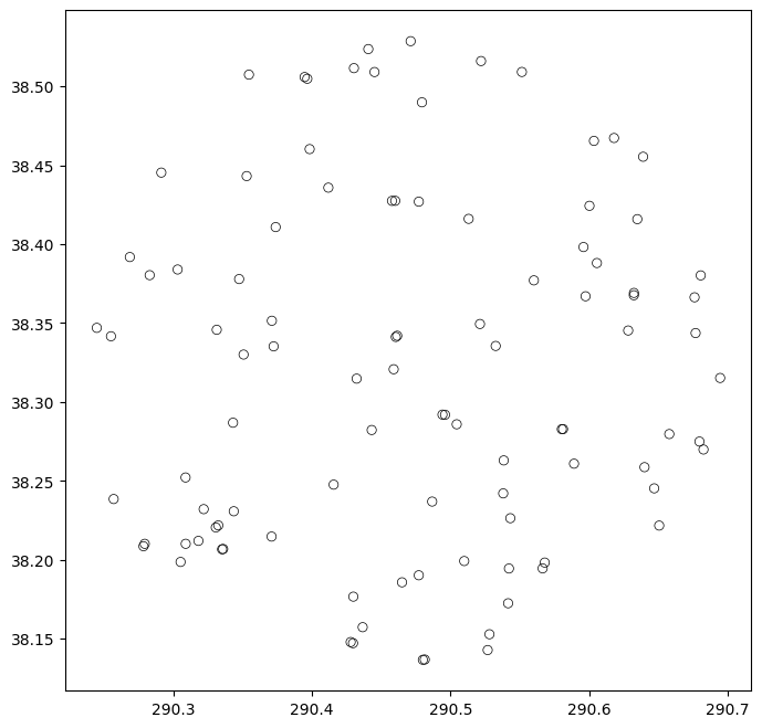
Let’s isolate the RA and Dec columns into a separate table for creating a plot. We will can also filter our results to include only sources brigther than 15 magnitudes in B, which will give us a more managable amount of sources for plotting:

radec = (catalogData['ra','dec','Bmag'])
mask = radec['Bmag'] < 15.0
mag_radec = radec[mask]
print(mag_radec)

       ra              dec         Bmag 
---------------- ---------------- ------
290.458960889796 38.3207432262466 14.795
      290.460477        38.341217  12.29
290.461502454307 38.3419735004403 12.282
290.432230727723 38.3148097580226 10.681
290.494195116716 38.2920041448032 13.699
290.496059793679 38.2919210910981 14.087
290.443098867166 38.2822568081951 14.969
290.521274498376 38.3494190597979 14.955
290.504480006636  38.285889095025 14.606
290.532642166954 38.3355127573579 14.949
             ...              ...    ...
290.639097732469 38.4553582786213 14.398
290.278293543156  38.208641997725 14.841
290.522060193556 38.5159651830843 13.833
290.551537246867 38.5090628454079 10.836
290.481412465678 38.1368775068458 14.623
290.480069981463 38.1366995602234 14.908
290.526845626658 38.1428874761665 13.564
 290.44065267106 38.5235618801004 13.479
290.354450995223 38.5073622260303 12.796
 290.47123419526 38.5285590704884 13.923
Length = 99 rows

We can plot this table to get an idea of what the catalog looks like visually:

fig = plt.figure(figsize=(8,8))
ax = fig.add_subplot(111)
plt.scatter(mag_radec['ra'], mag_radec['dec'], facecolors='none', edgecolors='k', linewidths=0.5)

<matplotlib.collections.PathCollection at 0x7f7dcdf854d0>

Top of Page

---

Overplotting Objects

Now that we have a way to display an FFI file and a catalog of objects, we can put the two pieces of data on the same plot. To do this, we will project the World Coordinate System (WCS) as a grid in units of degrees, minutes, and seconds onto the image. Then, we will create a scatter plot of the catalog, similar to the one above, although here we will transform its coordinate values into ICRS (International Celestial Reference System) to be compatible with the WCS projection:

hdu = fits.open(filename)[1]
wcs = WCS(hdu.header)

fig = plt.figure(figsize=(20,10))
ax = plt.subplot(projection=wcs) 
im = ax.imshow(hdu.data, cmap=plt.cm.gray, origin='lower', clim=(0,20000))
fig.colorbar(im)

plt.title('FFI with TIC Catalog Objects')
ax.set_xlabel('RA [deg]')
ax.set_ylabel('Dec [deg]')
ax.grid(color='white', ls='solid')
ax.autoscale(False)

ax.scatter(mag_radec['ra'], mag_radec['dec'],
           facecolors='none', edgecolors='c', linewidths=0.5,
           transform=ax.get_transform('icrs')) # This is needed when projecting onto axes with WCS info

WARNING: FITSFixedWarning: 'datfix' made the change 'Set MJD-OBS to 55001.173492 from DATE-OBS.
Set MJD-END to 55001.193926 from DATE-END'. [astropy.wcs.wcs]

<matplotlib.collections.PathCollection at 0x7f7d94dfd4d0>

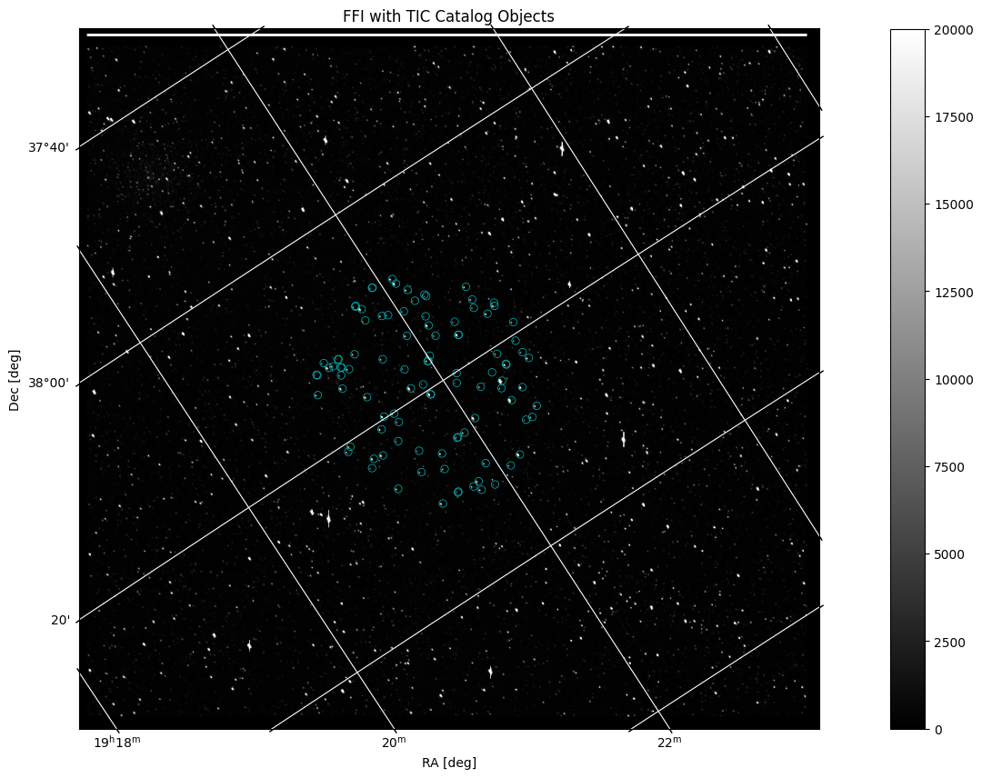
The catalog is displayed here as blue circles that highlight certain objects common in both the Kepler FFI and the TIC search. The image remains in x, y pixel values while the grid is projected in degrees based on the WCS. The projection works off of WCS data in the FFI header to create an accurate grid displaying RA and Dec coordinates that correspond to the original pixel values. The catalog data is transformed into ICRS coordinates in order to work compatibly with the other plotted data.

Top of Page

---

Aditional Resources

For more information about the MAST archive and details about mission data:

MAST API
Kepler Archive Page (MAST)
Kepler Archive Manual
Exo.MAST website
TESS Archive Page (MAST)

---

About this Notebook

Author: Josie Bunnell, STScI SASP Intern
Updated On: 08/13/2018

---

Top of Page