
Visualizing Periodic Signals Using a River Plot#
Learning Goals#
By the end of this tutorial, you will:
Understand what a river plot is.
Understand when river plots are useful.
Be able to create and interpret a river plot.
Introduction#
A “river plot” is a method to visualize periodic signals that vary over time. It is created by breaking a light curve into segments of equal length, such as the period of a planet orbiting a star, and displaying the segments side by side to allow the flux values to be compared. This allows you to examine how an entire light curve varies relative to a fixed period. It is similar to a “waterfall plot” which is used to similarly analyze time variation in spectra.
This tutorial demonstrates how to create a river plot using Lightkurve.
Imports#
This tutorial requires the Lightkurve package, which uses Matplotlib for plotting.
import lightkurve as lk
%matplotlib inline
1. When is a River Plot Useful?#
When we are looking for periodic signals in a light curve, sometimes it can be useful to see how they evolve over time. You can do this using the Lightkurve method plot_river on a FoldedLightCurve object.
We start by downloading some example data. We’ll use the target KIC 6185476, which is also known as KOI-227. This object exhibits strong transit timing variations (TTVs), that is, the transit time of the planet candidate changes over time. This happens when the orbit of a planet is not precisely periodic due to, for example, the presence of multiple moving stars or planets in the system.
We can use Lightkurve’s search_lightcurve function to get all of the available light curves from MAST and stitch them together.
lc = lk.search_lightcurve('KIC 6185476', cadence='long').download_all().stitch()
lc.plot();
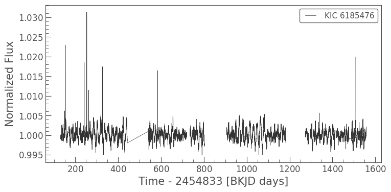
When we plot the data, we see that there is a long-term trend, likely from starspots. We can remove this with a Savitzky-Golay filter using Lightkurve’s flatten method.
clc = lc.flatten(21)
clc.plot();

The light curve is now flat. Let’s fold the light curve and plot it.
# Period (p) and and reference transit time (t0) are taken from the NASA Exoplanet Archive
p, t0 = 17.660114, 136.57258
folded_lc = clc.fold(period=p, epoch_time=t0)
folded_lc.scatter();
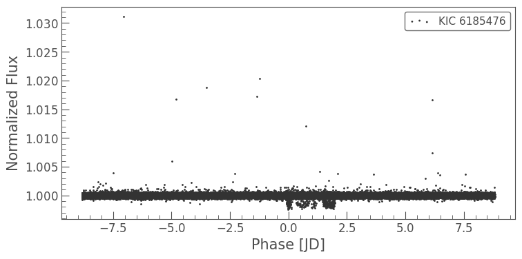
It looks like there is a concentration of points that are around phase of 0, but they don’t seem to line up nicely. This is caused by the transit of the planet occurring slightly before or after you would predict using a constant period. Cases of planets with meaningful TTVs are well suited for further analysis using a river plot.
2. Creating a River Plot#
We can use the plot_river method to plot the light curve in a more legible way. This must be performed on a folded LightCurve.
folded_lc.plot_river();
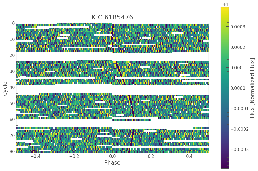
The river plot shows the same plot as the fold method, but each time the light curve is folded, a new row is started in the plot. The colorbar then shows the flux in each part of the light curve.
In this case we see a beautiful trend as the planet candidate orbit changes. In some cases, the signal won’t be this obvious. We can also use the plot_river method to bin in time to increase the signal to noise in any bin.
folded_lc.plot_river(bin_points=5, method='median');

3. Changing the Scale to Standard Deviation#
Finally, we can also use plot_river to look at the folded light curve in terms of standard deviation. This is useful when looking for signals that are of high significance.
folded_lc.plot_river(bin_points=1, method='sigma');
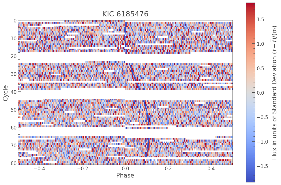
We see in the above river plot that there is a signal around phase of 0 (our planet candidate) that has a clear deviation from the mean, showing that it is a significant detection.
About this Notebook#
Authors: Christina Hedges (christinalouisehedges@gmail.com), Nicholas Saunders (nksaun@hawaii.edu)
Updated On: 2020-09-29
Citing Lightkurve and its Dependencies#
If you use lightkurve or its dependencies for published research, please cite the authors. Click the buttons below to copy BibTeX entries to your clipboard.
lk.show_citation_instructions()
When using Lightkurve, we kindly request that you cite the following packages:
- lightkurve
- astropy
- astroquery — if you are using search_lightcurve() or search_targetpixelfile().
- tesscut — if you are using search_tesscut().
