
Beginner: Read and Display a K2 Full Frame Image#
This notebook tutorial demonstrates how to load and display a K2 full frame image (FFI). We will display the image with the world coordinate system (WCS) overlayed on top.
Import Statements#
astropy.io.fits allows us to interact with the FITS files.
astropy.wcs.WCS allows us to interpret the world coordinate system.
matplotlib.pyplot is used to display the image.
numpy is used for array manipulation.
%matplotlib inline
from astropy.io import fits
from astropy.wcs import WCS
import matplotlib.pyplot as plt
import numpy as np
Introduction#
K2 reads out the entire frame of all its cameras once or twice per Campaign and stores them as full frame images. The total size on sky of the Kepler field-of-view is ~116 square degrees, although a few of the 21 modules had failed before the start of the K2 mission.
This tutorial will refer to a couple K2-related terms that we define here.
Campaign = During the K2 mission, the Kepler telescope observed the sky in a given pointing along the ecliptic plane for approximately 80 days at a time. Each of these regions is referred to as a “Campaign”, starting with Campaign 0 and ending with Campaign 19. There was also a special “Engineering” Campaign before Campaign 0 that lasted ~10 days.
HDU = Header Data Unit. A FITS file is made up of HDUs that contain data and metadata relating to the file. The first HDU is called the primary HDU, and anything that follows is considered an “extension”, e.g., “the first FITS extension”, “the second FITS extension”, etc.
BJD = Barycentric Julian Date, the Julian Date that has been corrected for differences in the Earth’s position with respect to the Solar System center of mass.
BKJD = Barycentric Kepler Julian Date, the timestamp measured in BJD, but offset by 2454833.0. I.e., BKJD = BJD - 2454833.0
WCS = World Coordinate System, A FITS convention used to store coordinate information inside FITS headers. For K2 full frame images, it is used to provide the translation needed to go from pixel coorindates to celestial coordinates in right ascension and declination.
Obtaining The Full Frame Image#
We will read the calibrated full frame image from Campaign 1 using the MAST URL location. So that we can get started with understanding the file contents without reviewing how to automatically search for and retrieve K2 files, we won’t show how to search and retrieve K2 FFIs in this tutorial.
# For the purposes of this tutorial, we just know the MAST URL location of the file we want to examine.
fits_file = "https://archive.stsci.edu/missions/k2/ffi/ktwo2015092174954-c04_ffi-cal.fits"
Understanding The FFI FITS File Structure#
K2 FFI FITS files contain a primary HDU with metadata stored in the header. There are then 84 extensions (21 modules * 4 channels per module) that contain more metadata in the header and stores the full frame image for that module+channel. Note that all 84 modules are included in the FFI FITS file, even if some of them do not have image data. Let’s examine the structure of the FITS file using the astropy.fits info function, which shows the FITS file format in more detail. Note this file is quite large and may take a few moments to dowload.
fits.info(fits_file)
Filename: /home/runner/.astropy/cache/download/url/7133df9c8b3174c962d802cbd0cc912a/contents
No.    Name      Ver    Type      Cards   Dimensions   Format
  0  PRIMARY       1 PrimaryHDU      60   ()
  1  MOD.OUT 2.1    1 ImageHDU       101   (1132, 1070)   float32
  2  MOD.OUT 2.2    1 ImageHDU       101   (1132, 1070)   float32
  3  MOD.OUT 2.3    1 ImageHDU       101   (1132, 1070)   float32
  4  MOD.OUT 2.4    1 ImageHDU       101   (1132, 1070)   float32
  5  MOD.OUT 3.1    1 ImageHDU        68   (1132, 1070)   float32
  6  MOD.OUT 3.2    1 ImageHDU        68   (1132, 1070)   float32
  7  MOD.OUT 3.3    1 ImageHDU        68   (1132, 1070)   float32
  8  MOD.OUT 3.4    1 ImageHDU        68   (1132, 1070)   float32
  9  MOD.OUT 4.1    1 ImageHDU       101   (1132, 1070)   float32
 10  MOD.OUT 4.2    1 ImageHDU       101   (1132, 1070)   float32
 11  MOD.OUT 4.3    1 ImageHDU       101   (1132, 1070)   float32
 12  MOD.OUT 4.4    1 ImageHDU       101   (1132, 1070)   float32
 13  MOD.OUT 6.1    1 ImageHDU       101   (1132, 1070)   float32
 14  MOD.OUT 6.2    1 ImageHDU       101   (1132, 1070)   float32
 15  MOD.OUT 6.3    1 ImageHDU       101   (1132, 1070)   float32
 16  MOD.OUT 6.4    1 ImageHDU       101   (1132, 1070)   float32
 17  MOD.OUT 7.1    1 ImageHDU        68   (1132, 1070)   float32
 18  MOD.OUT 7.2    1 ImageHDU        68   (1132, 1070)   float32
 19  MOD.OUT 7.3    1 ImageHDU        68   (1132, 1070)   float32
 20  MOD.OUT 7.4    1 ImageHDU        68   (1132, 1070)   float32
 21  MOD.OUT 8.1    1 ImageHDU       101   (1132, 1070)   float32
 22  MOD.OUT 8.2    1 ImageHDU       101   (1132, 1070)   float32
 23  MOD.OUT 8.3    1 ImageHDU       101   (1132, 1070)   float32
 24  MOD.OUT 8.4    1 ImageHDU       101   (1132, 1070)   float32
 25  MOD.OUT 9.1    1 ImageHDU       101   (1132, 1070)   float32
 26  MOD.OUT 9.2    1 ImageHDU       101   (1132, 1070)   float32
 27  MOD.OUT 9.3    1 ImageHDU       101   (1132, 1070)   float32
 28  MOD.OUT 9.4    1 ImageHDU       101   (1132, 1070)   float32
 29  MOD.OUT 10.1    1 ImageHDU       101   (1132, 1070)   float32
 30  MOD.OUT 10.2    1 ImageHDU       101   (1132, 1070)   float32
 31  MOD.OUT 10.3    1 ImageHDU       101   (1132, 1070)   float32
 32  MOD.OUT 10.4    1 ImageHDU       101   (1132, 1070)   float32
 33  MOD.OUT 11.1    1 ImageHDU       101   (1132, 1070)   float32
 34  MOD.OUT 11.2    1 ImageHDU       101   (1132, 1070)   float32
 35  MOD.OUT 11.3    1 ImageHDU       101   (1132, 1070)   float32
 36  MOD.OUT 11.4    1 ImageHDU       101   (1132, 1070)   float32
 37  MOD.OUT 12.1    1 ImageHDU       101   (1132, 1070)   float32
 38  MOD.OUT 12.2    1 ImageHDU       101   (1132, 1070)   float32
 39  MOD.OUT 12.3    1 ImageHDU       101   (1132, 1070)   float32
 40  MOD.OUT 12.4    1 ImageHDU       101   (1132, 1070)   float32
 41  MOD.OUT 13.1    1 ImageHDU       101   (1132, 1070)   float32
 42  MOD.OUT 13.2    1 ImageHDU       101   (1132, 1070)   float32
 43  MOD.OUT 13.3    1 ImageHDU       101   (1132, 1070)   float32
 44  MOD.OUT 13.4    1 ImageHDU       101   (1132, 1070)   float32
 45  MOD.OUT 14.1    1 ImageHDU       101   (1132, 1070)   float32
 46  MOD.OUT 14.2    1 ImageHDU       101   (1132, 1070)   float32
 47  MOD.OUT 14.3    1 ImageHDU       101   (1132, 1070)   float32
 48  MOD.OUT 14.4    1 ImageHDU       101   (1132, 1070)   float32
 49  MOD.OUT 15.1    1 ImageHDU       101   (1132, 1070)   float32
 50  MOD.OUT 15.2    1 ImageHDU       101   (1132, 1070)   float32
 51  MOD.OUT 15.3    1 ImageHDU       101   (1132, 1070)   float32
 52  MOD.OUT 15.4    1 ImageHDU       101   (1132, 1070)   float32
 53  MOD.OUT 16.1    1 ImageHDU       101   (1132, 1070)   float32
 54  MOD.OUT 16.2    1 ImageHDU       101   (1132, 1070)   float32
 55  MOD.OUT 16.3    1 ImageHDU       101   (1132, 1070)   float32
 56  MOD.OUT 16.4    1 ImageHDU       101   (1132, 1070)   float32
 57  MOD.OUT 17.1    1 ImageHDU       101   (1132, 1070)   float32
 58  MOD.OUT 17.2    1 ImageHDU       101   (1132, 1070)   float32
 59  MOD.OUT 17.3    1 ImageHDU       101   (1132, 1070)   float32
 60  MOD.OUT 17.4    1 ImageHDU       101   (1132, 1070)   float32
 61  MOD.OUT 18.1    1 ImageHDU       101   (1132, 1070)   float32
 62  MOD.OUT 18.2    1 ImageHDU       101   (1132, 1070)   float32
 63  MOD.OUT 18.3    1 ImageHDU       101   (1132, 1070)   float32
 64  MOD.OUT 18.4    1 ImageHDU       101   (1132, 1070)   float32
 65  MOD.OUT 19.1    1 ImageHDU       101   (1132, 1070)   float32
 66  MOD.OUT 19.2    1 ImageHDU       101   (1132, 1070)   float32
 67  MOD.OUT 19.3    1 ImageHDU       101   (1132, 1070)   float32
 68  MOD.OUT 19.4    1 ImageHDU       101   (1132, 1070)   float32
 69  MOD.OUT 20.1    1 ImageHDU       101   (1132, 1070)   float32
 70  MOD.OUT 20.2    1 ImageHDU       101   (1132, 1070)   float32
 71  MOD.OUT 20.3    1 ImageHDU       101   (1132, 1070)   float32
 72  MOD.OUT 20.4    1 ImageHDU       101   (1132, 1070)   float32
 73  MOD.OUT 22.1    1 ImageHDU       101   (1132, 1070)   float32
 74  MOD.OUT 22.2    1 ImageHDU       101   (1132, 1070)   float32
 75  MOD.OUT 22.3    1 ImageHDU       101   (1132, 1070)   float32
 76  MOD.OUT 22.4    1 ImageHDU       101   (1132, 1070)   float32
 77  MOD.OUT 23.1    1 ImageHDU       101   (1132, 1070)   float32
 78  MOD.OUT 23.2    1 ImageHDU       101   (1132, 1070)   float32
 79  MOD.OUT 23.3    1 ImageHDU       101   (1132, 1070)   float32
 80  MOD.OUT 23.4    1 ImageHDU       101   (1132, 1070)   float32
 81  MOD.OUT 24.1    1 ImageHDU       101   (1132, 1070)   float32
 82  MOD.OUT 24.2    1 ImageHDU       101   (1132, 1070)   float32
 83  MOD.OUT 24.3    1 ImageHDU       101   (1132, 1070)   float32
 84  MOD.OUT 24.4    1 ImageHDU       101   (1132, 1070)   float32
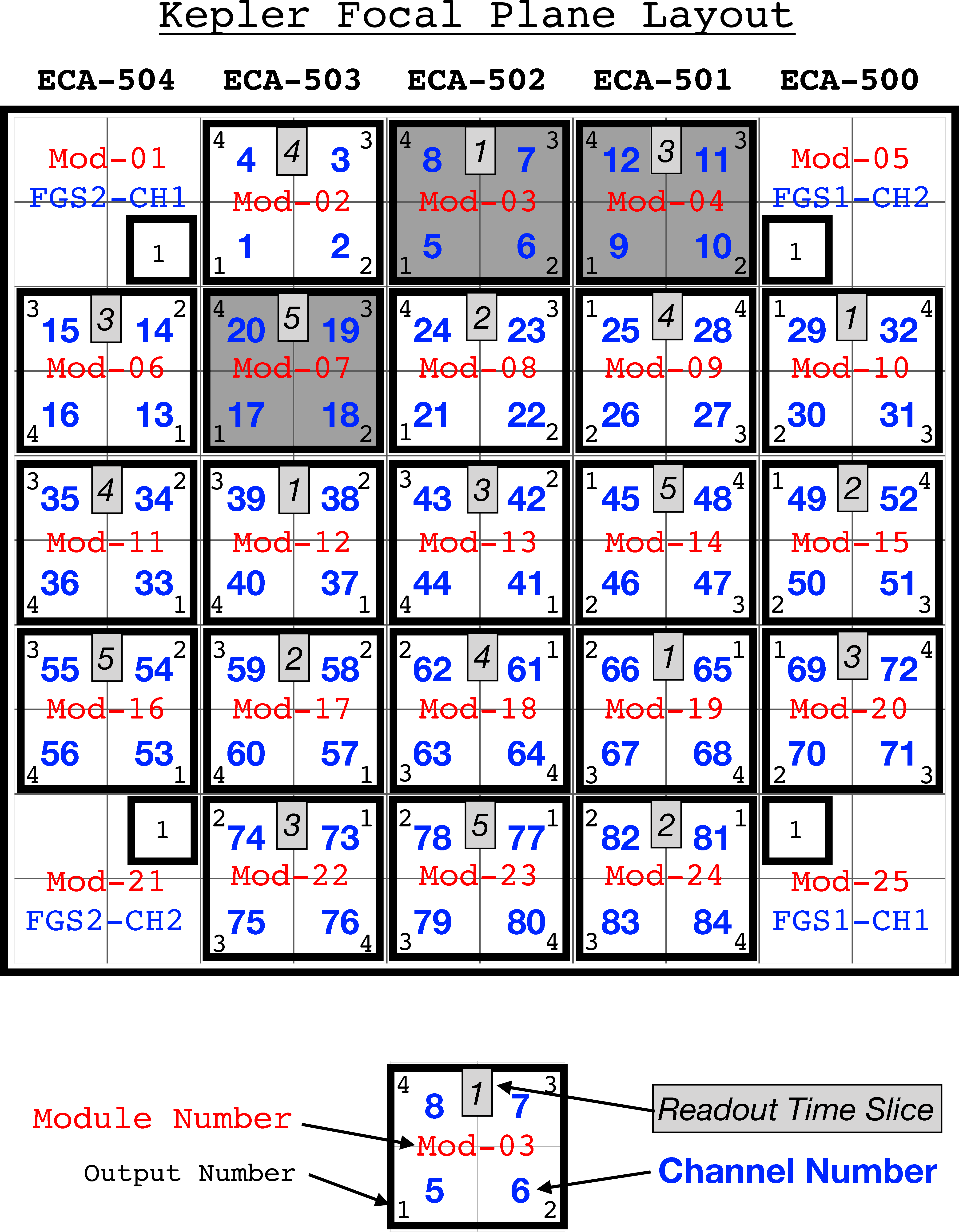
The image below shows the layout of the Kepler modules and channel numbers, for reference.
Reading the WCS and Calibrated Image#
Now that we have the file, let’s store the world coordinate system information for use later. We can use the astropy.wcs WCS function to store the information from the image extension HDU’s header.
The following command opens the file, extracts the WCS and Image data and then closes the file.
with fits.open(fits_file, mode = "readonly") as hdulist:
    wcs_info = WCS(hdulist[1].header)
    cal_image = hdulist[1].data
    header = hdulist[1].header
WARNING: FITSFixedWarning: 'datfix' made the change 'Set MJD-OBS to 57114.722560 from DATE-OBS.
Set MJD-END to 57114.742994 from DATE-END'. [astropy.wcs.wcs]
# Use the header to determine the mid-point of the exposure time for this FFI.
mid_time = (header['TSTOP'] + header['TSTART']) / 2
Display the Image#
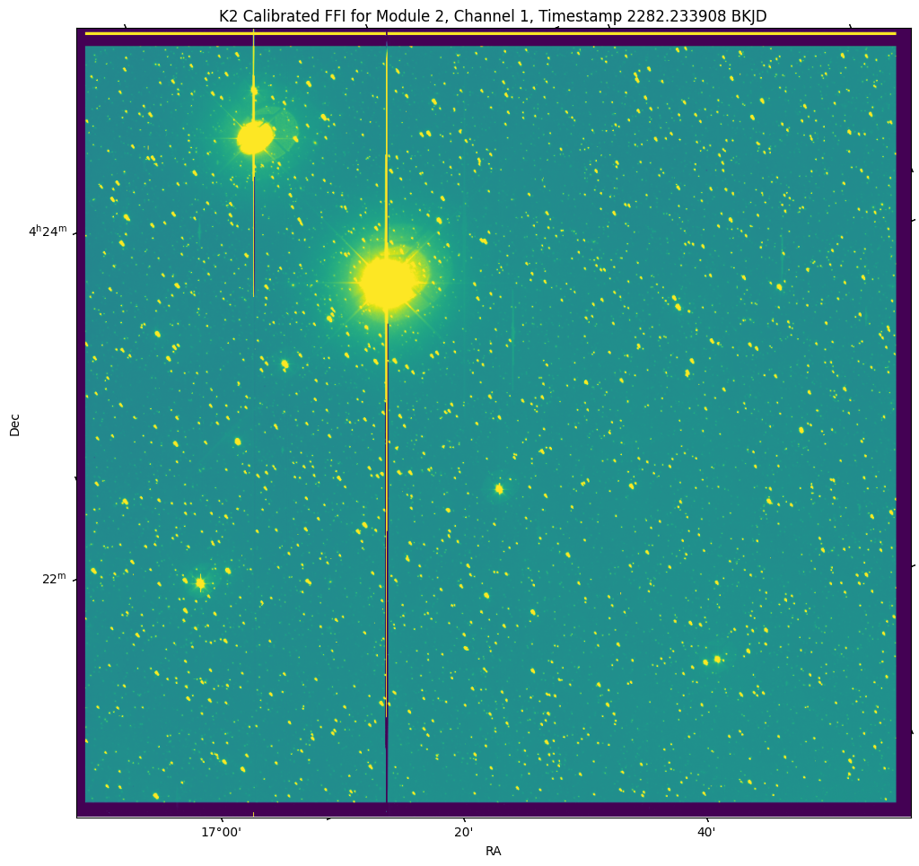
We show the full image from Module 2 Channel1, adjusting the scale so that we can see more of the stars. We also imprint the WCS on top of the image.
plt.figure(figsize = (12,12))

plt.subplot(111, projection = wcs_info)
plt.imshow(cal_image, vmin = np.percentile(cal_image,4),vmax = np.percentile(cal_image, 98),origin = "lower")
plt.xlabel('RA')
plt.ylabel('Dec')
plt.title("K2 Calibrated FFI for Module 2, Channel 1, Timestamp %f BKJD" % mid_time)
Text(0.5, 1.0, 'K2 Calibrated FFI for Module 2, Channel 1, Timestamp 2282.233908 BKJD')
A Few Image Details#
We describe some of the details you see on this FFI. For more detailed information please see the Kepler Instrument Handbook. Calibration row and columns are read-out in addition to the image data. These rows and columns remain in the calibrated image.
Leading and Trailing Black#
Each output channel have 12 columns for the “leading black” and 20 columns for the “trailing black”, used to determine reference levels and undershoot amplitudes.
Virtual, Smear and Buffer#
The top 26 rows are used to measure smear content, four of those rows are virtual rows, used to monitor undershoot and gain, and to clean out radiation traps.
About this Notebook#
Authors: Scott W. Fleming and Susan E. Mullally, STScI Archive Scientists
Updated On: 2019-01-30
