Hubble Catalog of Variables Notebook (CasJobs version)

This notebook shows how to access the Hubble Catalogs of Variables (HCV). The HCV is a large catalog of faint variable objects extracted from version 3 of the Hubble Source Catalog. The HCV project at the National Observatory of Athens was funded by the European Space Agency (PI: Alceste Bonanos). The data products for the HCV are available both at the ESA Hubble Archive at ESAC through the HCV Explorer interface and at STScI. See Bonanos et al. (2019) for more details.

Data tables in MAST CasJobs are queried from Python using the mastcasjobs module. For similar examples using the MAST API, which is easier to use but less powerful than CasJobs, see HCV_API_demo.

Instructions:

• Complete the initialization steps described below.

• Run the notebook to completion.

• Modify and rerun any sections of the Table of Contents below.

Table of Contents

• Intialization

• Variable objects in IC 1613

  • Name resolver

  • Select objects from HCV

  • Information on HCV variable classification

  • Sky coverage

  • Properties of variable objects

  • Color magnitude diagram

• Light curve for a nova in M87

  • Extract and plot light curve for the nova

  • HLA cutout images for selected measurements

• Compare the HCV automatic classification to expert validations

  • Plot MAD variability index distribution

  • Plot fraction of artifacts vs. MAD

• Plot light curve for most variable high-quality candidate in the HCV

Initialization

Install Python modules

1. This notebook requires the use of Python 3.

2. Modules can be installed with conda, if using the Anaconda distribution of python, or with pip.

   • If you are using conda, do not install / update / remove a module with pip, that exists in a conda channel.

   • If a module is not available with conda, then it’s okay to install it with pip

3. Install mastcasjobs and casjobs with pip:

pip install mastcasjobs

Set up your CasJobs account information

You must have a MAST Casjobs account. Note that MAST Casjobs accounts are independent of SDSS Casjobs accounts.

For easy startup, you can optionally set the environment variables CASJOBS_USERID and/or CASJOBS_PW with your Casjobs account information. The Casjobs user ID and password are what you enter when logging into Casjobs.

This script prompts for your Casjobs user ID and password during initialization if the environment variables are not defined.

import astropy
from astropy.coordinates import SkyCoord
import time
import sys
import os
import requests
import json
import numpy as np
import matplotlib.pyplot as plt

from PIL import Image
from io import BytesIO

from astropy.table import Table, join

# check that version of mastcasjobs is new enough
# we are using some features not in version 0.0.1
from pkg_resources import get_distribution
from packaging.version import Version as V

assert V(get_distribution("mastcasjobs").version) >= V('0.0.2'), """
A newer version of mastcasjobs is required.
Update mastcasjobs to current version using this command:
pip install --upgrade git+git://github.com/rlwastro/mastcasjobs@master
"""

import mastcasjobs

# set width for pprint
astropy.conf.max_width = 150

/tmp/ipykernel_2095/2985569151.py:18: DeprecationWarning: pkg_resources is deprecated as an API. See https://setuptools.pypa.io/en/latest/pkg_resources.html
  from pkg_resources import get_distribution

# set universal matplotlib parameters
plt.rcParams.update({'font.size': 16})

HSCContext = "HSCv3"

Set up Casjobs environment.

import getpass
if not os.environ.get('CASJOBS_USERID'):
    os.environ['CASJOBS_USERID'] = input('Enter Casjobs UserID:')
if not os.environ.get('CASJOBS_PW'):
    os.environ['CASJOBS_PW'] = getpass.getpass('Enter Casjobs password:')

Variable objects near IC 1613

Use astropy name resolver to get position of IC 1613

target = 'IC 1613'
coord_ic1613 = SkyCoord.from_name(target)

ra_ic1613 = coord_ic1613.ra.degree
dec_ic1613 = coord_ic1613.dec.degree
print(f'ra: {ra_ic1613}\ndec: {dec_ic1613}')

ra: 16.2016962
dec: 2.1194959

Select objects near IC 1613 with ACS F475W and F814W measurements from HCV

This searches the HCV summary table for objects within 0.5 degrees of the galaxy center. Note that this returns both variable and non-variable objects. We restrict the sample to objects with measurements in the two filters of interest. This uses the SearchHCVMatchID function to do the cone search.

DBtable = "HCV_demo"
jobs = mastcasjobs.MastCasJobs(context="MyDB")

# drop table if it already exists
jobs.drop_table_if_exists(DBtable)

# get main information
radius = 1800.0 # arcsec
query = f"""
select m.MatchID, m.GroupID, m.SubGroupID, m.RA, m.Dec,
   m.AutoClass, m.ExpertClass, m.NumFilters,
   f.Filter, f.FilterDetFlag, f.VarQualFlag, f.NumLC, 
   f.MeanMag, f.MeanCorrMag, f.MAD, f.Chi2
into mydb.{DBtable}
from SearchHCVMatchID({ra_ic1613},{dec_ic1613},{radius}) s
join HCVmatch m on m.MatchID=s.MatchID
join HCVfilter f on f.MatchID=s.MatchID and (f.Filter='ACS_F475W' or f.Filter='ACS_F814W')
"""

t0 = time.time()
results = jobs.quick(query, task_name="HCV demo", context=HSCContext)

print(f"Completed in {(time.time()-t0):.1f} sec")
print(results)

# fast retrieval using special MAST Casjobs service
tab = jobs.fast_table(DBtable, verbose=True)

# clean up the output format
tab['MeanMag'].format = "{:.3f}"
tab['MeanCorrMag'].format = "{:.3f}"
tab['MAD'].format = "{:.4f}"
tab['Chi2'].format = "{:.4f}"
tab['RA'].format = "{:.6f}"
tab['Dec'].format = "{:.6f}"

# show some of the variable sources
tab[tab['AutoClass'] > 0]

Completed in 2.5 sec
Rows Affected
-------------
        40196

1.5 s: Retrieved 6.34MB table MyDB.HCV_demo

1.8 s: Converted to 40196 row table

Table length=522

MatchID	GroupID	SubGroupID	RA	Dec	AutoClass	ExpertClass	NumFilters	Filter	FilterDetFlag	VarQualFlag	NumLC	MeanMag	MeanCorrMag	MAD	Chi2
int64	int32	int32	float64	float64	int32	int32	int32	str9	uint8	str5	int32	float64	float64	float64	float64
12131288	69810	-5	16.095659	2.161246	1	1	2	ACS_F475W	1	BACAA	12	25.248	25.250	0.1296	11.8544
12131288	69810	-5	16.095659	2.161246	1	1	2	ACS_F814W	0	AAAAC	12	25.215	25.217	0.0611	2.3024
82653722	69810	-5	16.097239	2.162066	2	1	2	ACS_F475W	1	AACAA	12	25.237	25.238	0.2312	64.6089
82653722	69810	-5	16.097239	2.162066	2	1	2	ACS_F814W	1	BACAA	12	25.069	25.070	0.1416	20.4986
100437228	69810	-5	16.111309	2.160908	2	1	2	ACS_F475W	1	ABCAA	12	23.249	23.249	0.1215	1231.5608
100437228	69810	-5	16.111309	2.160908	2	1	2	ACS_F814W	1	ABCAA	12	22.850	22.850	0.0719	329.2444
4358745	69810	-5	16.111961	2.157844	1	2	1	ACS_F475W	1	AACAA	7	26.108	26.111	0.1011	44.0548
78217904	69810	-5	16.110355	2.162592	2	1	2	ACS_F475W	1	AACAA	9	25.374	25.375	0.4343	44.1083
78217904	69810	-5	16.110355	2.162592	2	1	2	ACS_F814W	1	AACAB	9	25.189	25.189	0.1804	11.1780
...	...	...	...	...	...	...	...	...	...	...	...	...	...	...	...
99563258	69810	-5	16.101940	2.130867	1	4	2	ACS_F475W	1	AAAAC	12	23.926	23.927	0.0434	13.8320
99563258	69810	-5	16.101940	2.130867	1	4	2	ACS_F814W	0	ABAAC	11	22.550	22.551	0.0150	15.7979
26648962	69810	-5	16.104919	2.131477	2	1	2	ACS_F475W	1	AACBA	11	25.461	25.461	0.1582	19.5376
26648962	69810	-5	16.104919	2.131477	2	1	2	ACS_F814W	1	BAAAB	12	25.217	25.219	0.1019	5.4801
31257941	69810	-5	16.107393	2.128815	2	1	2	ACS_F475W	1	AACAA	12	23.168	23.168	0.0664	3751.2152
31257941	69810	-5	16.107393	2.128815	2	1	2	ACS_F814W	1	AACAA	12	22.885	22.887	0.0862	814.8062
14005460	69810	-5	16.109657	2.127282	2	1	2	ACS_F475W	1	AACCA	12	25.470	25.470	0.1774	56.3907
14005460	69810	-5	16.109657	2.127282	2	1	2	ACS_F814W	1	AACAA	10	25.248	25.250	0.1241	16.0616
57557150	69810	-5	16.108461	2.128060	2	1	2	ACS_F475W	1	AACAA	12	25.319	25.319	0.1391	18.9906
57557150	69810	-5	16.108461	2.128060	2	1	2	ACS_F814W	1	AABAC	12	25.319	25.320	0.0877	4.2321

Description of the variable classification columns

Several of the table columns have information on the variability.

• The columns AutoClass and ExpertClass have summary information on the variability for a given MatchID object.

  • AutoClass: Classification as provided by the system: 0=constant 1=single filter variable candidate (SFVC) 2=multi-filter variable candidate (MFVC)

  • ExpertClass: Classification as provided by expert: 0=not classified by expert, 1=high confidence variable, 2=probable variable, 4=possible artifact

• The columns MAD and Chi2 are variability indices using the median absolute deviation and the \(\chi^2\) parameter for the given filter.

• The column VarQualFlag is a variability quality flag (see Section 5 of the paper). The five letters correspond to CI, D, MagerrAper2, MagAper2-MagAuto, p2p; AAAAA corresponds to the highest quality flag.

• The column FilterDetFlag is the filter detection flag: 1=source is variable in this filter, 0=source is not variable in this filter.

See the HCV paper by Bonanos et al. (2019, AAp) for more details on the computation and meaning of these quantities.

Find objects with measurements in both F475W and F814W

This could also be done in the SQL query. Here we use the Astropy.table.join function instead.

# the only key needed to do the join is MatchID, but we include other common columns
# so that join includes only one copy of them
jtab = join(tab[tab['Filter'] == 'ACS_F475W'], tab[tab['Filter'] == 'ACS_F814W'],
            keys=['MatchID', 'GroupID', 'SubGroupID', 'RA', 'Dec', 'AutoClass', 'ExpertClass'],
            table_names=['f475', 'f814'])
print(len(jtab), "matched F475W+F814W objects")
jtab[jtab['AutoClass'] > 0]

17090 matched F475W+F814W objects

Table length=258

MatchID	GroupID	SubGroupID	RA	Dec	AutoClass	ExpertClass	NumFilters_f475	Filter_f475	FilterDetFlag_f475	VarQualFlag_f475	NumLC_f475	MeanMag_f475	MeanCorrMag_f475	MAD_f475	Chi2_f475	NumFilters_f814	Filter_f814	FilterDetFlag_f814	VarQualFlag_f814	NumLC_f814	MeanMag_f814	MeanCorrMag_f814	MAD_f814	Chi2_f814
int64	int32	int32	float64	float64	int32	int32	int32	str9	uint8	str5	int32	float64	float64	float64	float64	int32	str9	uint8	str5	int32	float64	float64	float64	float64
96457	69810	-5	16.141516	2.177815	2	1	2	ACS_F475W	1	AACAA	12	23.192	23.192	0.0686	424.7097	2	ACS_F814W	1	AAAAC	12	22.946	22.947	0.0402	77.5733
813653	69810	-5	16.128353	2.160147	1	4	2	ACS_F475W	0	AAAAC	10	25.508	25.507	0.0243	0.2945	2	ACS_F814W	1	BACAB	11	24.906	24.908	0.0795	8.5797
1012692	69810	-5	16.134809	2.144720	2	1	2	ACS_F475W	1	AACAA	7	25.439	25.438	0.1446	17.9867	2	ACS_F814W	1	AABAB	8	25.208	25.210	0.1152	6.6471
1085386	69810	-5	16.118544	2.160845	1	4	2	ACS_F475W	0	AAAAC	11	24.351	24.352	0.0174	3.1311	2	ACS_F814W	1	BABBB	11	23.476	23.476	0.0697	40.7630
1286857	69810	-5	16.119205	2.184252	1	2	2	ACS_F475W	1	AABAB	12	23.137	23.138	0.0477	53.2282	2	ACS_F814W	0	AAAAC	12	21.073	21.075	0.0128	46.8982
1309271	69810	-5	16.130571	2.152512	2	1	2	ACS_F475W	1	AACAA	12	25.347	25.348	0.1399	20.0434	2	ACS_F814W	1	AAAAC	12	25.043	25.044	0.0804	5.2954
1479646	69810	-5	16.120852	2.152737	1	2	2	ACS_F475W	0	CACAA	12	23.691	23.692	0.0332	41.9525	2	ACS_F814W	1	AABAB	12	22.501	22.503	0.0362	68.2414
1661315	69810	-5	16.110571	2.143526	1	4	2	ACS_F475W	1	AACAB	12	25.220	25.221	0.0780	5.8648	2	ACS_F814W	0	AAAAC	12	25.887	25.889	0.0595	0.8037
1826474	69810	-5	16.101532	2.171855	1	2	2	ACS_F475W	0	AAAAC	11	25.735	25.737	0.0259	0.5195	2	ACS_F814W	1	BACAB	11	24.889	24.890	0.0822	9.2131
...	...	...	...	...	...	...	...	...	...	...	...	...	...	...	...	...	...	...	...	...	...	...	...	...
102132800	69810	-5	16.126160	2.145442	2	1	2	ACS_F475W	1	AACAA	12	23.691	23.692	0.0750	129.5717	2	ACS_F814W	1	AACBA	12	24.503	24.505	0.1038	27.1660
102239423	69810	-5	16.138706	2.155652	1	2	2	ACS_F475W	1	AABAA	12	22.810	22.811	0.0982	307.5226	2	ACS_F814W	0	AABAA	12	22.735	22.737	0.0382	96.9001
103232694	69810	-5	16.107565	2.174399	1	4	2	ACS_F475W	0	AAAAC	11	22.422	22.422	0.0060	1.7118	2	ACS_F814W	1	AAAAC	11	22.425	22.426	0.0335	27.9930
104300195	69810	-5	16.124981	2.171772	2	1	2	ACS_F475W	1	AACAA	12	25.540	25.541	0.1054	58.7587	2	ACS_F814W	1	AACAA	12	25.382	25.384	0.1217	9.4811
105173757	69810	-5	16.133703	2.184506	2	1	2	ACS_F475W	1	AAAAA	12	21.372	21.372	0.1589	2810.1572	2	ACS_F814W	1	AACAA	12	22.240	22.242	0.1825	829.2399
106466795	69810	-5	16.127056	2.166390	1	1	2	ACS_F475W	1	AACAA	12	25.357	25.358	0.1425	13.4065	2	ACS_F814W	0	AAAAC	12	25.257	25.259	0.0462	2.8032
106640363	69810	-5	16.135796	2.149099	1	2	2	ACS_F475W	1	CACAA	8	25.577	25.579	0.1161	5.8168	2	ACS_F814W	0	AABAB	9	24.944	24.946	0.0661	8.3312
106843213	69810	-5	16.110342	2.150373	1	4	2	ACS_F475W	0	CACCB	12	23.691	23.691	0.0269	30.7690	2	ACS_F814W	1	CACBA	12	24.429	24.431	0.0710	25.8158
107834538	69810	-5	16.107105	2.160084	1	1	2	ACS_F475W	1	AABAC	12	25.400	25.401	0.0818	3.4254	2	ACS_F814W	0	AAAAC	12	25.128	25.129	0.0578	1.7916
108048053	69810	-5	16.150572	2.142590	1	2	2	ACS_F475W	1	AACCA	10	25.297	25.297	0.0697	22.9085	2	ACS_F814W	0	AAAAC	11	24.544	24.546	0.0273	1.6361

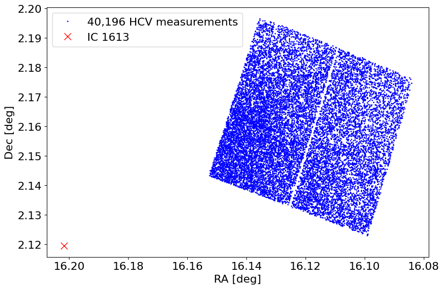
Plot object positions on the sky

We mark the galaxy center as well. Note that this field is in the outskirts of IC 1613. The 0.5 degree search radius (which is the maximum allowed in the API) allows finding these objects.

fig, ax = plt.subplots(figsize=(10, 10))
ax.plot('RA', 'Dec', 'bo', markersize=1, label=f'{len(tab):,} HCV measurements', data=jtab)
ax.plot(ra_ic1613, dec_ic1613, 'rx', label=target, markersize=10)
ax.invert_xaxis()
ax.set(aspect='equal', xlabel='RA [deg]', ylabel='Dec [deg]')
ax.legend(loc='best')

<matplotlib.legend.Legend at 0x7f42b74b6050>

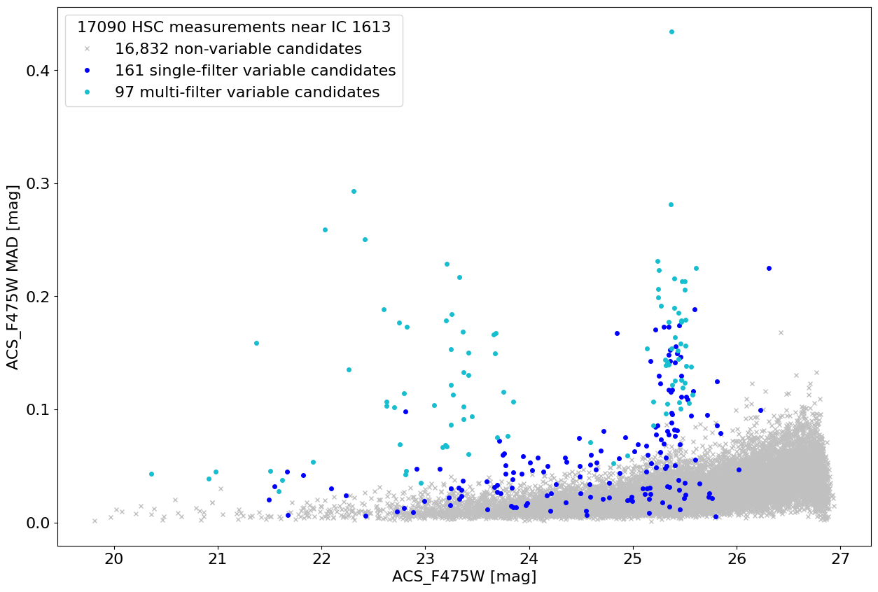
Plot HCV MAD variability index versus magnitude in F475W

The median absolute deviation variability index is used by the HCV to identify variables. It measures the scatter among the multi-epoch measurements. Some scatter is expected from noise (which increases for fainter objects). Objects with MAD values that are high are likely to be variable.

This plots single-filter and multi-filter variable candidates (SFVC and MFVC) in different colors. Note that variable objects with low F475W MAD values are variable in a different filter (typically F814W in this field).

This plot is similar to the upper panel of Figure 4 in Bonanos et al. (2019, AAp).

# define plot parameter lists
auto_class = np.unique(jtab['AutoClass'])
markers = ['x', 'o', 'o']
colors = ['silver', 'blue', 'tab:cyan']
labels = ['non-', 'single-filter ', 'multi-filter ']

fig, ax = plt.subplots(figsize=(15, 10))
for ac, marker, color, label in zip(auto_class, markers, colors, labels):
    data = jtab[jtab['AutoClass'] == ac]
    ax.plot('MeanCorrMag_f475', 'MAD_f475', marker, markersize=4, color=color,
            label=f'{len(data):,} {label}variable candidates', data=data)

ax.set(xlabel='ACS_F475W [mag]', ylabel='ACS_F475W MAD [mag]')
ax.legend(loc='best', title=f'{len(jtab)} HSC measurements near {target}')

<matplotlib.legend.Legend at 0x7f42bc399b10>

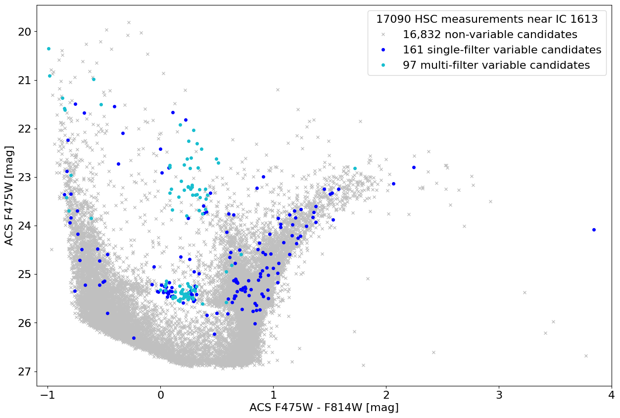
Plot variables in color-magnitude diagram

Many of the candidate variables lie on the instability strip.

This plot is similar to the lower panel of Figure 4 in Bonanos et al. (2019, AAp).

# add a new column to jtab
jtab['MCMf475-MCMf814'] = jtab['MeanCorrMag_f475'] - jtab['MeanCorrMag_f814']

fig, ax = plt.subplots(figsize=(15, 10))
# uses same plot parameters defined in the previous plot
for ac, marker, color, label in zip(auto_class, markers, colors, labels):
    data = jtab[jtab['AutoClass'] == ac]
    ax.plot('MCMf475-MCMf814', 'MeanCorrMag_f475', marker, markersize=4, color=color,
            label=f'{len(data):,} {label}variable candidates', data=data)
    
ax.invert_yaxis()
ax.set(xlim=(-1.1, 4), xlabel='ACS F475W - F814W [mag]', ylabel='ACS F475W [mag]')
ax.legend(loc='best', title=f'{len(jtab)} HSC measurements near {target}')

<matplotlib.legend.Legend at 0x7f42b4b02d10>

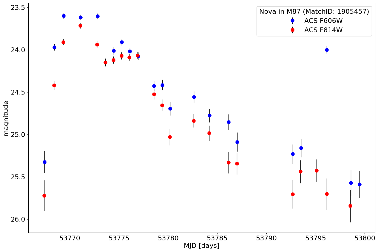
Get a light curve for a nova in M87

Extract light curve for a given MatchID

Note that the MatchID could be determined by positional searches, filtering the catalog, etc. This object comes from the top left panel of Figure 9 in Bonanos et al. (2019, AAp).

matchid = 1905457

jobs = mastcasjobs.MastCasJobs(context=HSCContext)
t0 = time.time()

# get light curves for F606W and F814W
nova_606 = jobs.quick(f"""select * from HCVdetailed
where MatchID={matchid} and Filter='ACS_F606W'""", task_name="HCV demo")
print(f"{(time.time()-t0):.1f} sec: retrieved {len(nova_606)} F606W measurements")

nova_814 = jobs.quick("""select * from HCVdetailed
where MatchID={} and Filter='ACS_F814W'
""".format(matchid), task_name="HCV demo")
print(f"{(time.time()-t0):.1f} sec: retrieved {len(nova_814)} F814W measurements")

# get the object RA and Dec as well
nova_tab = jobs.quick(f"""select MatchID, RA, Dec from HCVmatch
where MatchID={matchid}""", task_name="HCV demo")
print(f"{(time.time()-t0):.1f} sec: retrieved object info")

nova_606

0.5 sec: retrieved 21 F606W measurements

1.0 sec: retrieved 22 F814W measurements

1.6 sec: retrieved object info

Table length=21

MatchID	Filter	MJD	ImageName	Mag	CorrMag	MagErr	CI	D
int64	str9	float64	str26	float64	float64	float64	float64	float64
1905457	ACS_F606W	53767.4197952871	hst_10543_29_acs_wfc_f606w	25.327	25.3267132802993	0.1305	0.840648114681244	13.499119758606
1905457	ACS_F606W	53768.4190663833	hst_10543_30_acs_wfc_f606w	23.9694	23.9676109802196	0.0394	1.04379630088806	11.9895544052124
1905457	ACS_F606W	53769.3576541713	hst_10543_31_acs_wfc_f606w	23.6005	23.6000842124737	0.0306	0.974166631698608	9.30478286743164
1905457	ACS_F606W	53771.1017052617	hst_10543_33_acs_wfc_f606w	23.6105	23.6157510517543	0.030300001	0.96657407283783	2.96933674812317
1905457	ACS_F606W	53772.8098534283	hst_10543_35_acs_wfc_f606w	23.621799	23.602993885395	0.0328	0.992037057876587	4.45478820800781
1905457	ACS_F606W	53774.4746564087	hst_10543_37_acs_wfc_f606w	24.015499	24.0123868023881	0.042599998	1.0246297121048	3.4874792098999
1905457	ACS_F606W	53775.2799112014	hst_10543_38_acs_wfc_f606w	23.9037	23.9077547341058	0.0381	0.985185205936432	3.49740219116211
1905457	ACS_F606W	53776.0893441574	hst_10543_39_acs_wfc_f606w	24.015499	24.0182108840315	0.0414	1.05314815044403	8.44466972351074
1905457	ACS_F606W	53776.9439852673	hst_10543_40_acs_wfc_f606w	24.065701	24.0743889490328	0.044599999	1.24157404899597	7.6749701499939
1905457	ACS_F606W	53778.562434162	hst_10543_42_acs_wfc_f606w	24.430799	24.4274937224049	0.059500001	1.07425928115845	3.26662158966064
1905457	ACS_F606W	53779.4097260174	hst_10543_43_acs_wfc_f606w	24.415899	24.4150584573105	0.062600002	0.965277791023254	2.09669971466064
1905457	ACS_F606W	53780.2090778507	hst_10543_44_acs_wfc_f606w	24.697599	24.6944838119623	0.080499999	0.810648143291473	6.5630521774292
1905457	ACS_F606W	53782.61915897	hst_10543_47_acs_wfc_f606w	24.560801	24.5570748994592	0.065399997	1.09907412528992	2.88692712783813
1905457	ACS_F606W	53784.2176541714	hst_10543_73_acs_wfc_f606w	24.7827	24.7770110702267	0.079000004	0.888148188591003	3.16040587425232
1905457	ACS_F606W	53786.1563230369	hst_10543_86_acs_wfc_f606w	24.9091	24.8532684587691	0.0902	1.03777778148651	8.54914951324463
1905457	ACS_F606W	53787.0225386124	hst_10543_92_acs_wfc_f606w	25.114599	25.0878230960564	0.1127	0.924444437026978	4.14372444152832
1905457	ACS_F606W	53792.6850963715	hst_10543_49_acs_wfc_f606w	25.228001	25.231832236643	0.1147	1.14425933361053	11.9895496368408
1905457	ACS_F606W	53793.5260915786	hst_10543_a1_acs_wfc_f606w	25.153601	25.1604359861786	0.1071	0.925648152828217	7.5528678894043
1905457	ACS_F606W	53796.1486378878	hst_10543_b8_acs_wfc_f606w	24.0172	23.9985920051837	0.0436	1.51175928115845	10.1193161010742
1905457	ACS_F606W	53798.5892174062	hst_10543_50_acs_wfc_f606w	25.563601	25.5708965234736	0.15350001	0.953240752220154	12.9010400772095
1905457	ACS_F606W	53799.4608942058	hst_10543_c4_acs_wfc_f606w	25.5895	25.5908707417737	0.1602	0.92981481552124	5.97602415084839

fig, ax = plt.subplots(figsize=(15, 10))

ax.errorbar(x='MJD', y='CorrMag', yerr='MagErr', fmt='ob', ecolor='k', elinewidth=1, markersize=8, label='ACS F606W', data=nova_606)
ax.errorbar(x='MJD', y='CorrMag', yerr='MagErr', fmt='or', ecolor='k', elinewidth=1, markersize=8, label='ACS F814W', data=nova_814)

ax.invert_yaxis()
ax.set(xlabel='MJD [days]', ylabel='magnitude')
ax.legend(loc='best', title=f'Nova in M87 (MatchID: {matchid})')

<matplotlib.legend.Legend at 0x7f42b74ea990>

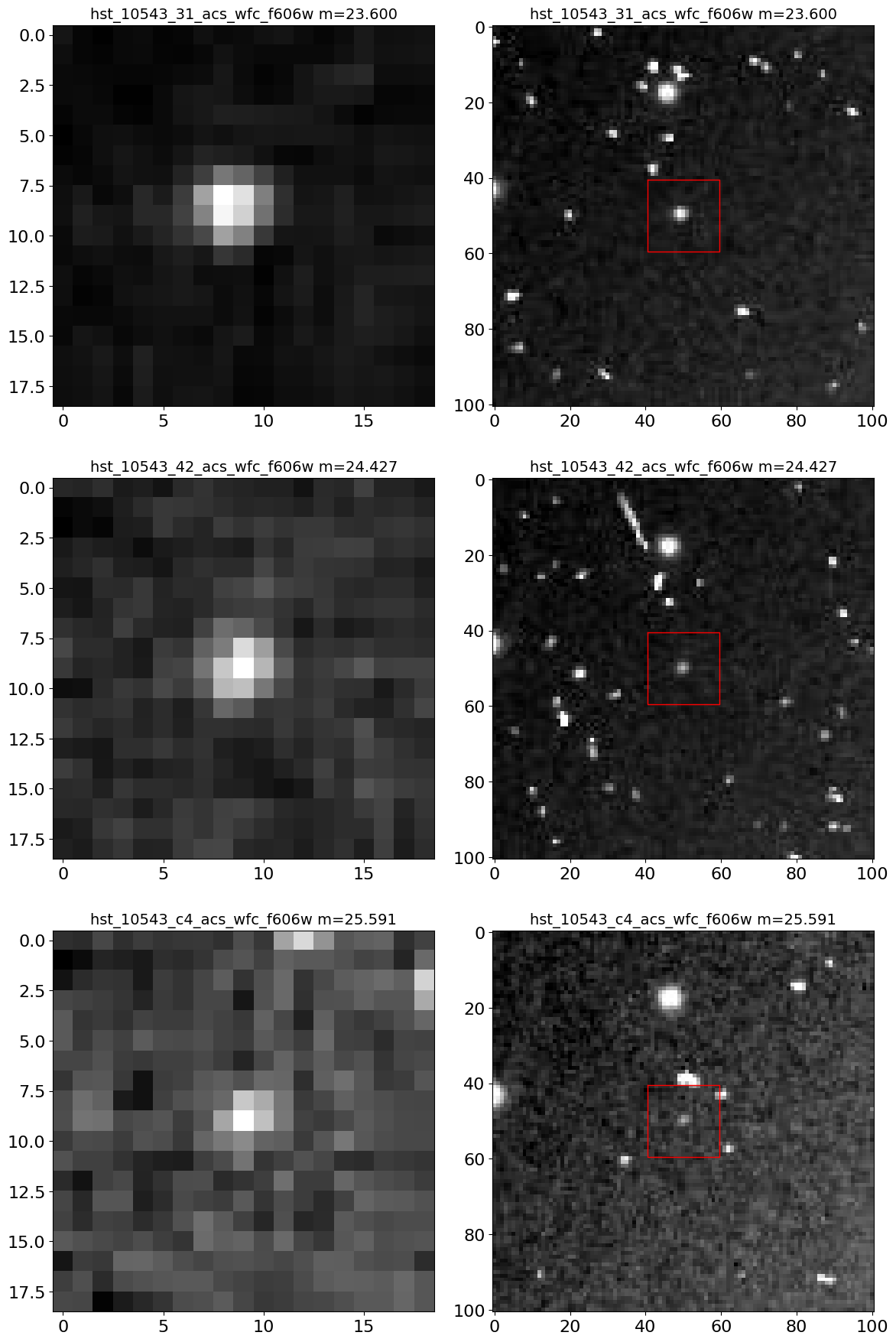
Get HLA image cutouts for the nova

The Hubble Legacy Archive (HLA) images were the source of the measurements in the HSC and HCV, and it can be useful to look at the images. Examination of the images can be useful to identified cosmic-ray contamination and other possible image artifacts. In this case, no issues are seen, so the light curve is reliable.

Note that the ACS F606W images of M87 have only a single exposure, so they do have cosmic ray contamination. The accompanying F814W images have multiple exposures, allowing CRs to be removed. In this case the F814W combined image is used to find objects, while the F606W exposure is used only for photometry. That reduces the effects of F606W CRs on the catalog but it is still a good idea to confirm the quality of the images.

The get_hla_cutout function reads a single cutout image (as a JPEG grayscale image) and returns a PIL image object. See the documentation on the fitscut image cutout service for more information on the web service being used.

def get_hla_cutout(imagename, ra, dec, size=33, autoscale=99.5, asinh=True, zoom=1):
    """Get JPEG cutout for an image"""
    url = "https://hla.stsci.edu/cgi-bin/fitscut.cgi"
    r = requests.get(url, params=dict(ra=ra, dec=dec, size=size, format="jpeg",
                                      red=imagename, autoscale=autoscale, asinh=asinh, zoom=zoom))
    im = Image.open(BytesIO(r.content))
    return im

# sort images by magnitude from brightest to faintest
phot = nova_606
isort = np.argsort(phot['CorrMag'])
# select the brightest, median and faintest magnitudes
ind = [isort[0], isort[len(isort)//2], isort[-1]]

# we plot zoomed-in and zoomed-out views side-by-side for each selected image
nim = len(ind)*2
ncols = 2 # images per row
nrows = (nim+ncols-1)//ncols

imsize1 = 19
imsize2 = 101
mra = nova_tab['RA'][0]
mdec = nova_tab['Dec'][0]

# define figure and axes
fig, axes = plt.subplots(nrows, ncols, figsize=(12, (12/ncols)*nrows), tight_layout=True)

t0 = time.time()

# iterate through each set of two subplots in axes
for (ax1, ax2), k in zip(axes, ind):
    
    # get the images
    im1 = get_hla_cutout(phot['ImageName'][k], mra, mdec, size=imsize1)
    im2 = get_hla_cutout(phot['ImageName'][k], mra, mdec, size=imsize2)
    
    # plot left column   
    ax1.imshow(im1, origin="upper", cmap="gray")
    ax1.set_title(f"{phot['ImageName'][k]} m={phot['CorrMag'][k]:.3f}", fontsize=14)
    
    # plot right column
    ax2.imshow(im2, origin="upper", cmap="gray")
    xbox = np.array([-1, 1])*imsize1/2 + (imsize2-1)//2
    ax2.plot(xbox[[0, 1, 1, 0, 0]], xbox[[0, 0, 1, 1, 0]], 'r-', linewidth=1)
    ax2.set_title(f"{phot['ImageName'][k]} m={phot['CorrMag'][k]:.3f}", fontsize=14)    
    
print(f"{(time.time()-t0):.1f} s: got {nrows*ncols} cutouts")

6.2 s: got 6 cutouts

Compare the HCV automatic classification to expert validations

The HCV includes an automatic classification AutoClass for candidate variables as well as an expert validation for some fields that were selected for visual examination. See the description of the classification columns and the HCV paper by Bonanos et al. (2019, AAp) for more details on the computation and meaning of these quantities.

For this example, we select all the objects in the HCV that have expert classification information.

DBtable = "HCV_demo2"
jobs = mastcasjobs.MastCasJobs(context="MyDB")

# drop table if it already exists
jobs.drop_table_if_exists(DBtable)

# get data for objects with an expert validation
query = f"""
select m.MatchID, m.GroupID, m.SubGroupID, m.RA, m.Dec,
   m.AutoClass, m.ExpertClass, m.NumFilters,
   f.Filter, f.FilterDetFlag, f.VarQualFlag, f.NumLC, 
   f.MeanMag, f.MeanCorrMag, f.MAD, f.Chi2
into mydb.{DBtable}
from HCVmatch m
join HCVfilter f on m.MatchID=f.MatchID
where m.ExpertClass>0
"""

t0 = time.time()
results = jobs.quick(query, task_name="HCV demo", context=HSCContext)

print(f"Completed in {(time.time()-t0):.1f} sec")
print(results)

# fast retrieval using special MAST Casjobs service
tab = jobs.fast_table(DBtable, verbose=True)

# clean up the output format
tab['MeanMag'].format = "{:.3f}"
tab['MeanCorrMag'].format = "{:.3f}"
tab['MAD'].format = "{:.4f}"
tab['Chi2'].format = "{:.4f}"
tab['RA'].format = "{:.6f}"
tab['Dec'].format = "{:.6f}"

# tab includes 1 row for each filter (so multiple rows for objects with multiple filters)
# get an array that has only one row per object
mval, uindex = np.unique(tab['MatchID'], return_index=True)
utab = tab[uindex]
print(f"{len(utab)} unique MatchIDs in table")

tab

Completed in 0.9 sec
Rows Affected
-------------
        31258

1.6 s: Retrieved 4.94MB table MyDB.HCV_demo2

1.8 s: Converted to 31258 row table
13533 unique MatchIDs in table

Table length=31258

MatchID	GroupID	SubGroupID	RA	Dec	AutoClass	ExpertClass	NumFilters	Filter	FilterDetFlag	VarQualFlag	NumLC	MeanMag	MeanCorrMag	MAD	Chi2
int64	int32	int32	float64	float64	int32	int32	int32	str11	uint8	str5	int32	float64	float64	float64	float64
875	1040153	-5	64.149673	-24.110353	2	2	7	ACS_F435W	0	AAAAA	13	24.166	24.166	0.0384	7.1169
875	1040153	-5	64.149673	-24.110353	2	2	7	ACS_F606W	0	AAAAC	9	22.836	22.835	0.0349	81.3676
875	1040153	-5	64.149673	-24.110353	2	2	7	ACS_F814W	0	AAAAA	23	22.156	22.156	0.0325	141.7171
875	1040153	-5	64.149673	-24.110353	2	2	7	WFC3_F105W	1	CAAAB	14	21.843	21.843	0.0503	223.4961
875	1040153	-5	64.149673	-24.110353	2	2	7	WFC3_F125W	1	CBCCA	6	21.813	21.814	0.0655	792.8662
875	1040153	-5	64.149673	-24.110353	2	2	7	WFC3_F140W	0	AAAAA	6	21.705	21.704	0.0205	127.6242
875	1040153	-5	64.149673	-24.110353	2	2	7	WFC3_F160W	1	BABAA	13	21.623	21.624	0.0322	112.8544
2006	521507	-5	268.112152	-17.684282	2	2	2	WFPC2_F555W	1	AAAAC	7	21.811	21.821	0.1545	85.2812
2006	521507	-5	268.112152	-17.684282	2	2	2	WFPC2_F814W	1	AAAAA	7	20.513	20.519	0.0988	105.2348
...	...	...	...	...	...	...	...	...	...	...	...	...	...	...	...
108116850	1045904	85	11.627593	42.061874	1	1	2	ACS_F475W	0	AAAAA	5	24.772	24.774	0.0498	52.0622
108116850	1045904	85	11.627593	42.061874	1	1	2	ACS_F814W	1	AACAA	5	24.605	24.607	0.1120	56.7844
108127522	1043478	-5	211.154297	54.521580	1	1	1	ACS_F606W	1	AACAA	6	26.786	26.786	0.1496	12.5680
108141967	1036556	-5	34.188431	-5.203189	1	4	2	ACS_F606W	1	BAACA	5	26.174	26.175	0.1806	5.3338
108141967	1036556	-5	34.188431	-5.203189	1	4	2	ACS_F814W	0	AAAAC	5	25.970	25.969	0.0561	0.2748
108154109	1084533	-5	53.141266	-27.710630	1	2	5	ACS_F606W	0	CAAAC	7	24.477	24.477	0.0161	3.4616
108154109	1084533	-5	53.141266	-27.710630	1	2	5	ACS_F775W	0	CAAAC	11	23.650	23.650	0.0588	2.6932
108154109	1084533	-5	53.141266	-27.710630	1	2	5	ACS_F814W	0	CAAAC	5	23.577	23.577	0.0037	2.9994
108154109	1084533	-5	53.141266	-27.710630	1	2	5	ACS_F850LP	1	CAAAA	12	23.455	23.455	0.0639	3.4468
108154109	1084533	-5	53.141266	-27.710630	1	2	5	WFC3_F105W	0	AAAAC	6	21.541	21.541	0.0065	0.4013

An ExpertClass value of 1 indicates that the object is confidently confirmed to be a variable; 2 means that the measurements do not have apparent problems and so the object is likely to be variable (usually the variability is too small to be obvious in the image); 4 means that the variability is likely to be the result of artifacts in the image (e.g., residual cosmic rays or diffraction spikes from nearby bright stars).

Compare the distributions for single-filter variable candidates (SFVC, AutoClass=1) and multi-filter variable candidates (MFVC, AutoClass=2). The fraction of artifacts is lower in the MFVC sample.

sfcount = np.bincount(utab['ExpertClass'][utab['AutoClass'] == 1])
mfcount = np.bincount(utab['ExpertClass'][utab['AutoClass'] == 2])
sfrat = sfcount/sfcount.sum()
mfrat = mfcount/mfcount.sum()

print("Type Variable Likely Artifact Total")
print("SFVC {:8d} {:6d} {:8d} {:5d} counts".format(sfcount[1], sfcount[2], sfcount[4], sfcount.sum()))
print("MFVC {:8d} {:6d} {:8d} {:5d} counts".format(mfcount[1], mfcount[2], mfcount[4], mfcount.sum()))
print("SFVC {:8.3f} {:6.3f} {:8.3f} {:5.3f} fraction".format(sfrat[1], sfrat[2], sfrat[4], sfrat.sum()))
print("MFVC {:8.3f} {:6.3f} {:8.3f} {:5.3f} fraction".format(mfrat[1], mfrat[2], mfrat[4], mfrat.sum()))

Type Variable Likely Artifact Total
SFVC     3323   3055     1761  8139 counts
MFVC     2101   2442      851  5394 counts
SFVC    0.408  0.375    0.216 1.000 fraction
MFVC    0.390  0.453    0.158 1.000 fraction

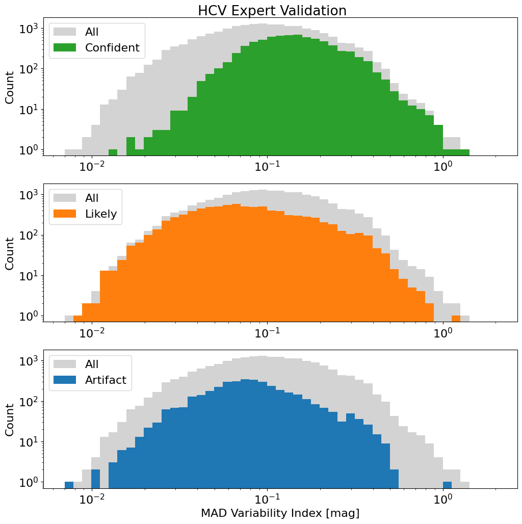
Plot the MAD variability index distribution with expert classifications

Note that only the filters identified as variable (FilterDetFlag > 0) are included here.

This version of the plot shows the distributions for the various ExpertClass values along with, for comparison, the distribution for all objects in gray (which is identical in each panel). Most objects are classified as confident or likely variables. Objects with lower MAD values (indicating a lower amplitude of variability) are less likely to be identified as confident variables because low-level variability is more difficult to confirm via visual examination.

Data & Bins

w = np.where(tab['FilterDetFlag'] > 0)
mad = tab['MAD'][w]
e = tab['ExpertClass'][w]

xrange = [7.e-3, 2.0]
bins = xrange[0]*(xrange[1]/xrange[0])**np.linspace(0.0, 1.0, 50)

Plots

fig, axes = plt.subplots(3, 1, figsize=(12, 12))

labels = ['Confident', 'Likely', 'Artifact']
colors = ['C2', 'C1', 'C0']

for ax, v, label, color in zip(axes, np.unique(e), labels, colors):
    ax.hist(mad, bins=bins, log=True, color='lightgray', label='All')
    ax.hist(mad[e == v], bins=bins, log=True, label=label, color=color)
    ax.set(xscale='log', ylabel='Count')
    ax.legend(loc='upper left')
    
fig.suptitle('HCV Expert Validation', y=0.9)
_ = axes[2].set_xlabel('MAD Variability Index [mag]')

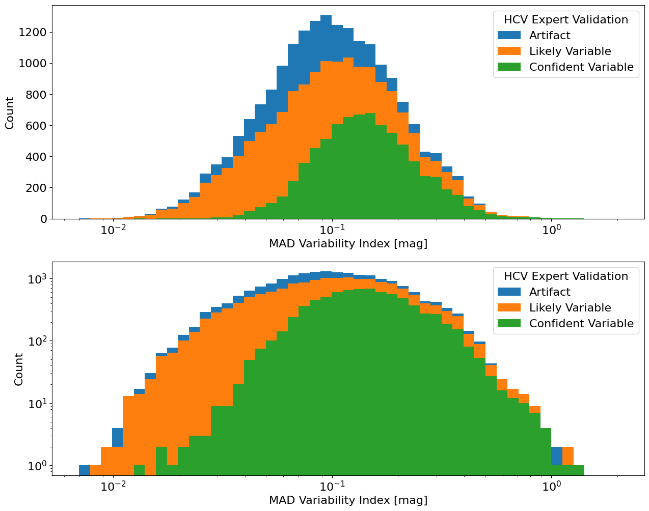
The plot below shows the same distributions, but plotted as stacked histograms. The top panel uses a linear scale on the y-axis and the bottom panel uses a log y scale.

fig, axes = plt.subplots(2, 1, figsize=(15, 12))

ylogs = [False, True]

for ax, ylog in zip(axes, ylogs):
    ax.hist(mad, bins=bins, log=ylog, label='Artifact')
    ax.hist(mad[e < 4], bins=bins, log=ylog, label='Likely Variable')
    ax.hist(mad[e == 1], bins=bins, log=ylog, label='Confident Variable')

    ax.set_xscale('log')
    ax.set_xlabel('MAD Variability Index [mag]')
    ax.set_ylabel('Count')
    ax.legend(loc='upper right', title='HCV Expert Validation')

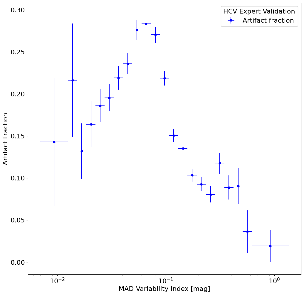
Plot the fraction of artifacts as a function of MAD variability index

This shows how the fraction of artifacts varies with the MAD value. For larger MAD values the fraction decreases sharply, presumably because such large values are less likely to result from the usual artifacts. Interestingly, the artifact fraction also declines for smaller MAD values (MAD < 0.1 mag). Probably that happens because typical artifacts are more likely to produce strong signals than the weaker signals indicated by a low MAD value.

w = np.where(tab['FilterDetFlag'] > 0)
mad = tab['MAD'][w]
e = tab['ExpertClass'][w]

xrange = [7.e-3, 2.0]
bins = xrange[0]*(xrange[1]/xrange[0])**np.linspace(0.0, 1.0, 30)

all_count, bin_edges = np.histogram(mad, bins=bins)
artifact_count, bin_edges = np.histogram(mad[e == 4], bins=bins)
wnz = np.where(all_count > 0)[0]
nnz = len(wnz)

artifact_count = artifact_count[wnz]
all_count = all_count[wnz]
xerr = np.empty((2, nnz), dtype=float)
xerr[0] = bin_edges[wnz]
xerr[1] = bin_edges[wnz+1]

# combine bins at edge into one big bin to improve the statistics there
iz = np.where(all_count.cumsum() > 10)[0][0]
if iz > 0:
    all_count[iz] += all_count[:iz].sum()
    artifact_count[iz] += artifact_count[:iz].sum()
    xerr[0, iz] = xerr[0, 0]
    all_count = all_count[iz:]
    artifact_count = artifact_count[iz:]
    xerr = xerr[:, iz:]
    
iz = np.where(all_count[::-1].cumsum() > 40)[0][0]
if iz > 0:
    all_count[-iz-1] += all_count[-iz:].sum()
    artifact_count[-iz-1] = artifact_count[-iz:].sum()
    xerr[1, -iz-1] = xerr[1, -1]
    all_count = all_count[:-iz]
    artifact_count = artifact_count[:-iz]
    xerr = xerr[:, :-iz]

x = np.sqrt(xerr[0]*xerr[1])
xerr[0] = x - xerr[0]
xerr[1] = xerr[1] - x

frac = artifact_count/all_count
# error on fraction using binomial distribution (approximate)
ferr = np.sqrt(frac*(1-frac)/all_count)

Create the plot

fig, ax = plt.subplots(figsize=(12, 12))
ax.errorbar(x, frac, xerr=xerr, yerr=ferr, fmt='ob', markersize=5, label='Artifact fraction')
ax.set(xscale='log', xlabel='MAD Variability Index [mag]', ylabel='Artifact Fraction')
ax.legend(loc='upper right', title='HCV Expert Validation')

<matplotlib.legend.Legend at 0x7f42b72b23d0>

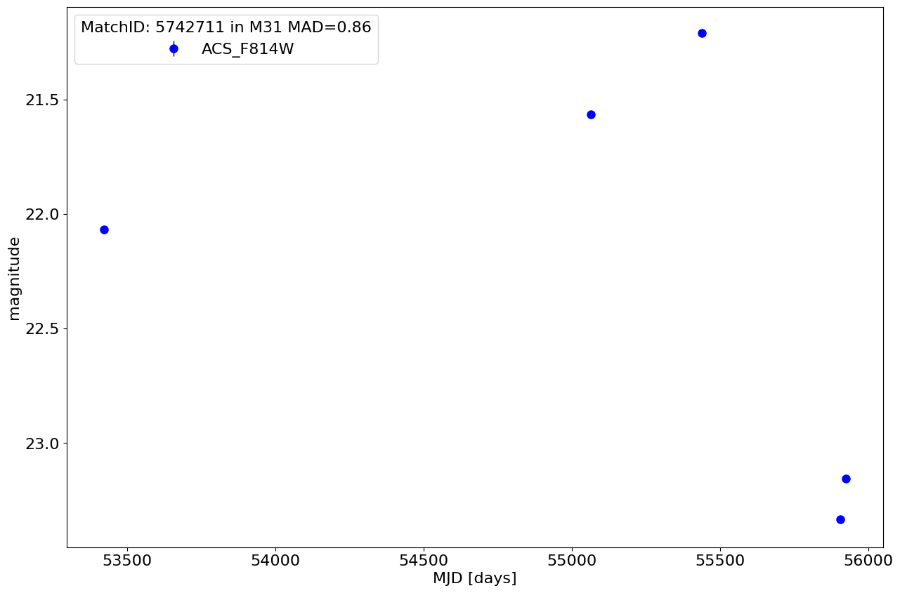
Plot light curve for the most variable high quality candidate in the HCV

Select the candidate variable with the largest MAD value and VarQualFlag = ‘AAAAA’. To find the highest MAD value, we sort by MAD in descending order and select the first result.

jobs = mastcasjobs.MastCasJobs(context=HSCContext)

# join to the Groups table as well to get the target name

query = """
select top 1 m.MatchID, m.GroupID, m.SubGroupID, g.TargetName, m.RA, m.Dec,
   m.AutoClass, m.ExpertClass, m.NumFilters,
   f.Filter, f.FilterDetFlag, f.VarQualFlag, f.NumLC, 
   f.MeanMag, f.MeanCorrMag, f.MAD, f.Chi2
from HCVmatch m
join HCVfilter f on m.MatchID=f.MatchID
join Groups g on m.GroupID=g.GroupID
where f.VarQualFlag='AAAAA'
order by f.MAD desc
"""

t0 = time.time()
tab = jobs.quick(query, task_name="HCV demo", context=HSCContext)

print(f"Completed in {(time.time()-t0):.1f} sec")

# clean up the output format
tab['MeanMag'].format = "{:.3f}"
tab['MeanCorrMag'].format = "{:.3f}"
tab['MAD'].format = "{:.4f}"
tab['Chi2'].format = "{:.4f}"
tab['RA'].format = "{:.6f}"
tab['Dec'].format = "{:.6f}"

print(f"MatchID {tab['MatchID'][0]} in group '{tab['TargetName'][0]}' has largest MAD value = {tab['MAD'][0]:.2f}")
tab

Completed in 1.1 sec
MatchID 5742711 in group 'M31' has largest MAD value = 0.86

Table length=1

MatchID	GroupID	SubGroupID	TargetName	RA	Dec	AutoClass	ExpertClass	NumFilters	Filter	FilterDetFlag	VarQualFlag	NumLC	MeanMag	MeanCorrMag	MAD	Chi2
int64	int64	int64	str3	float64	float64	int64	int64	int64	str9	str4	str5	int64	float64	float64	float64	float64
5742711	1045904	16	M31	10.928601	41.164295	1	0	1	ACS_F814W	True	AAAAA	5	22.264	22.265	0.8581	6698.4430

Get the light curve.

matchid = tab['MatchID'][0]
mfilter = tab['Filter'][0]

jobs = mastcasjobs.MastCasJobs(context=HSCContext)
t0 = time.time()

# get light curves for F606W and F814W
lc = jobs.quick("""select * from HCVdetailed
where MatchID={} and Filter='{}'
""".format(matchid, mfilter), task_name="HCV demo")
print(f"{(time.time()-t0):.1f} sec: retrieved {len(lc)} {mfilter} measurements")

0.5 sec: retrieved 5 ACS_F814W measurements

Plot the light curve.

fig, ax = plt.subplots(figsize=(15, 10))

ax.errorbar(x='MJD', y='CorrMag', yerr='MagErr', fmt='ob', ecolor='k', elinewidth=1, markersize=8, label=mfilter, data=lc)

ax.invert_yaxis()
ax.set(xlabel='MJD [days]', ylabel='magnitude')
ax.legend(loc='best', title=f"MatchID: {matchid} in {tab['TargetName'][0]} MAD={tab['MAD'][0]:.2f}")

<matplotlib.legend.Legend at 0x7f42b701a6d0>

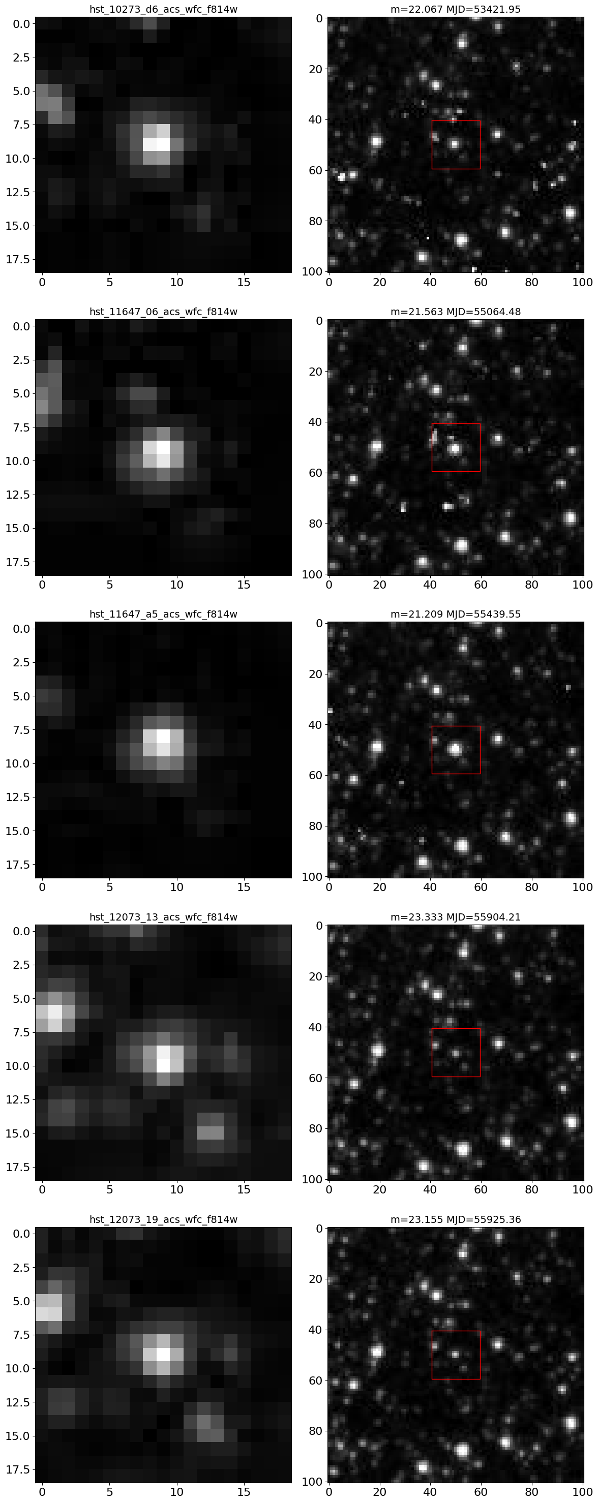
Extract cutout images for the entire light curve (since it does not have many points).

# sort images in MJD order
ind = np.argsort(lc['MJD'])

# we plot zoomed-in and zoomed-out views side-by-side for each selected image
nim = len(ind)*2
ncols = 2 # images per row
nrows = (nim+ncols-1)//ncols

imsize1 = 19
imsize2 = 101
mra = tab['RA'][0]
mdec = tab['Dec'][0]

# define figure and axes
fig, axes = plt.subplots(nrows, ncols, figsize=(12, (12/ncols)*nrows), tight_layout=True)

t0 = time.time()

# iterate through each set of two subplots in axes
for i, ((ax1, ax2), k) in enumerate(zip(axes, ind), 1):
    
    # get the images
    im1 = get_hla_cutout(lc['ImageName'][k], mra, mdec, size=imsize1)
    im2 = get_hla_cutout(lc['ImageName'][k], mra, mdec, size=imsize2)
    
    # plot left column    
    ax1.imshow(im1, origin="upper", cmap="gray")
    ax1.set_title(lc['ImageName'][k], fontsize=14)
    
    # plot right column
    ax2.imshow(im2, origin="upper", cmap="gray")
    xbox = np.array([-1, 1])*imsize1/2 + (imsize2-1)//2
    ax2.plot(xbox[[0, 1, 1, 0, 0]], xbox[[0, 0, 1, 1, 0]], 'r-', linewidth=1)
    ax2.set_title(f"m={lc['CorrMag'][k]:.3f} MJD={lc['MJD'][k]:.2f}", fontsize=14)
    
    print(f"{(time.time()-t0):.1f} s: finished {i} of {len(ind)} epochs")
    
print(f"{(time.time()-t0):.1f} s: got {nrows*ncols} cutouts")

1.9 s: finished 1 of 5 epochs

3.8 s: finished 2 of 5 epochs

5.7 s: finished 3 of 5 epochs

7.4 s: finished 4 of 5 epochs

9.3 s: finished 5 of 5 epochs
9.3 s: got 10 cutouts

About this Notebook

If you have comments or questions on this notebook, please contact us through the Archive Help Desk e-mail at archive@stsci.edu.

Author(s): Rick White, Steve Lubow, Trenton McKinney
Last Updated: May 2023

---

Top of Page