MRS Cube Analysis#
Use case: Extract spatial-spectral features from IFU cube and measure their attributes.
Data: Simulated MIRI MRS spectrum of AGB star.
Tools: specutils, jwst, photutils, astropy, scipy.
Cross-intrument: NIRSpec, MIRI.
Documentation: This notebook is part of a STScI’s larger post-pipeline Data Analysis Tools Ecosystem and can be downloaded directly from the JDAT Notebook Github directory.
Source of Simulations: MIRISim
Pipeline Version: JWST Pipeline
Note: This notebook includes MIRI simulated data cubes obtained using MIRISim (https://wiki.miricle.org//bin/view/Public/MIRISim_Public) and run through the JWST pipeline (https://jwst-pipeline.readthedocs.io/en/latest/) of point sources with spectra representative of late M type stars.
Introduction#
This notebook analyzes one star represented by a dusty SED corresponding to the ISO SWS spectrum of W Per from Kraemer et al. (2002) and Sloan et al. (2003) to cover the MRS spectral range 5-28 microns. Analysis of JWST spectral cubes requires extracting spatial-spectral features of interest and measuring their attributes.
This is the second notebook, which will perform data analysis using specutils. Specifically, it will fit a model photosphere/blackbody to the spectra. Then it will calculate the centroids, line integrated flux and equivalent width for each dust and molecular feature.
This notebook utilizes reduced data created in the first notebook (JWST_Mstar_dataAnalysis_runpipeline.ipynb), although you don’t have to run that notebook to use this notebook. All data created in notebook number 1 are available for download within this noteobok.
To Do:#
Make function to extract spectra from datacube using a different means of extraction.
Replace blackbody fit to the photosphere part of the spectra with a stellar photosphere model.
Make sure errors have been propagated correctly in the caculation of centroids, line integrated flux and equivalent widths. (Science Author)
Make simple function within the
specutilsframework to fit a continium and measure centroids, line integrated flux and equivalent widths of broad solid state and molecular features.
Import Packages#
# Import useful python packages
import numpy as np

# Import packages to display images inline in the notebook
import matplotlib.pyplot as plt
%matplotlib inline

# Set general plotting options
params = {'legend.fontsize': '18', 'axes.labelsize': '18',
          'axes.titlesize': '18', 'xtick.labelsize': '18',
          'ytick.labelsize': '18', 'lines.linewidth': 2, 'axes.linewidth': 2, 'animation.html': 'html5'}
plt.rcParams.update(params)
plt.rcParams.update({'figure.max_open_warning': 0})
# Import astropy packages
from astropy import units as u
from astropy.io import ascii
from astropy.nddata import StdDevUncertainty
from astropy.utils.data import download_file

# To deal with 1D spectrum
from specutils import Spectrum1D
from specutils.manipulation import box_smooth, extract_region
from specutils.analysis import line_flux, centroid, equivalent_width
from specutils.spectra import SpectralRegion
from specutils import SpectrumList
from jdaviz import Specviz
from jdaviz import Cubeviz

# Display the video
from IPython.display import HTML, YouTubeVideo
# Save and Load Objects Using Pickle
import pickle


def save_obj(obj, name):
    with open(name, 'wb') as f:
        pickle.dump(obj, f, pickle.HIGHEST_PROTOCOL)


def load_obj(name):
    with open(name, 'rb') as f:
        return pickle.load(f)
def checkKey(dict, key):

    if key in dict.keys():
        print("Present, ", end=" ")
        print("value =", dict[key])
        return True
    else:
        print("Not present")
        return False
import warnings
warnings.simplefilter('ignore')
# Check if Pipeline 3 Reduced data exists and, if not, download it
import os
import urllib.request

if os.path.exists("combine_dithers_all_exposures_ch1-long_s3d.fits"):
    print("Pipeline 3 Data Exists")
else:
    url = 'https://data.science.stsci.edu/redirect/JWST/jwst-data_analysis_tools/MRS_Mstar_analysis/reduced.tar.gz'
    urllib.request.urlretrieve(url, './reduced.tar.gz')
    # Unzip Tar Files

    import tarfile

    # Unzip files if they haven't already been unzipped
    if os.path.exists("reduced/"):
        print("Pipeline 3 Data Exists")
    else:
        tar = tarfile.open('./reduced.tar.gz', "r:gz")
        tar.extractall()
        tar.close()

    # Move Files
    os.system('mv reduced/*fits .')
Pipeline 3 Data Exists
Read in 12 spectra from Notebook 1 using SpectrumList and create one master spectrum. MIRI MRS data will typically have a separate 1D spectrum and 3D cube associated with each Channel and Sub-Band.
# Read in all X1D spectra to a single spectrum list and combine into a single spectrum1d object

ddd = '.'
splist = SpectrumList.read(ddd)

wlallorig = []
fnuallorig = []
dfnuallorig = []
for bndind in range(len(splist)):
    for wlind in range(len(splist[bndind].spectral_axis)):
        wlallorig.append(splist[bndind].spectral_axis[wlind].value)
        fnuallorig.append(splist[bndind].flux[wlind].value)
        dfnuallorig.append(splist[bndind].uncertainty[wlind].array)

wlallarr = np.array(wlallorig)
fnuallarr = np.array(fnuallorig)
dfnuallarr = np.array(dfnuallorig)
srtind = np.argsort(wlallarr)
wlall = wlallarr[srtind]
fnuall = fnuallarr[srtind]

# Developer Note: We put in errors of 0.0001, but uncertainties need to be fixed
dfnuall = (0.0001)*np.ones(len(fnuall))
Specviz Visualization of the SpectrumList#
You can visualize the spectrum list inside a Jupyter notebook using Specviz
Video 1:#
This Specviz Instructional Demo is from STScI’s official YouTube channel and provides an introduction to Specviz.
vid = YouTubeVideo("zLyRnfG32Bo")
display(vid)
Read in the SpectrumList (12 unique spectra)#
# Open these spectra up in Specviz
specviz = Specviz()
specviz.show()
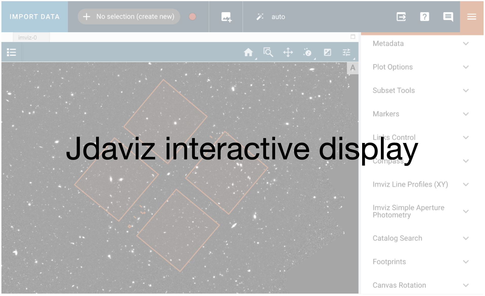
Cubeviz Visualization#
You can also visualize images inside a Jupyter notebook using Cubeviz
Video 2:#
This Cubeviz Instructional Demo is from STScI’s official YouTube channel and provides an introduction to Cubeviz.
vid = YouTubeVideo("HMSYwiH3Gl4")
display(vid)
cubeviz = Cubeviz()
cubeviz.show()
Developer Note. Need to pick a different unit than meters. https://jira.stsci.edu/browse/JDAT-1792#
# Here, we load the data into the Cubeviz app for visual inspection.
# In this case, we're just looking at a single channel because, unlike Specviz, Cubeviz can only load a single cube at a time.

ch1short_cubefile = 'combine_dithers_all_exposures_ch1-long_s3d.fits'
cubeviz.load_data(ch1short_cubefile)
Next, you want to define a pixel region subset that is specific to the AGB star. You can do this with the regions utility button shown in the video below and drawing a circular region around the AGB star at approximate pixels x=20, y=30.
Video 3:#
Here is a video that quickly shows how to select a spatial region in Cubeviz.
# Video showing the selection of the star with a circular region of interest
HTML('<iframe width="700" height="500" src="https://data.science.stsci.edu/redirect/JWST/jwst-data_analysis_tools/MRS_Mstar_analysis/region_select.mov" frameborder="0" allowfullscreen></iframe>')
# Now extract spectrum from your spectral viewer
try:
    spec_agb = cubeviz.get_data('combine_dithers_all_exposures_ch1-long_s3d[SCI]',
                                spatial_subset='Subset 1', function='mean') # AGB star only
    print(spec_agb)
    spec_agb_exists = True
except Exception:
    print("There are no subsets selected.")
    spec_agb_exists = False
    spec_agb = cubeviz.get_data('combine_dithers_all_exposures_ch1-long_s3d[SCI]',
                                function='mean') # Whole field of view
There are no subsets selected.
Developer Note: Since Cubeviz only displays a single cube at a time, you can’t extract a full spectrum at the current time. So, you should use the spectrum defined above (‘spec’)#
Make a 1D spectrum object#
wav = wlall*u.micron # Wavelength: microns
fl = fnuall*u.Jy # Fnu:  Jy
efl = dfnuall*u.Jy # Error flux: Jy

# Make a 1D spectrum object
spec = Spectrum1D(spectral_axis=wav, flux=fl, uncertainty=StdDevUncertainty(efl))
# Apply a 5 pixel boxcar smoothing to the spectrum
spec_bsmooth = box_smooth(spec, width=5)
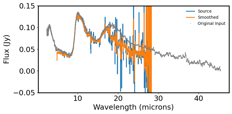
# Plot the spectrum & smoothed spectrum to inspect features
plt.figure(figsize=(8, 4))
plt.plot(spec.spectral_axis, spec.flux, label='Source')
plt.plot(spec.spectral_axis, spec_bsmooth.flux, label='Smoothed')
plt.xlabel('Wavelength (microns)')
plt.ylabel("Flux ({:latex})".format(spec.flux.unit))
plt.ylim(-0.05, 0.15)
# Overplot the original input spectrum for comparison
origspecfile = fn = download_file('https://data.science.stsci.edu/redirect/JWST/jwst-data_analysis_tools/MRS_Mstar_analysis/63702662.txt', cache=True)
origdata = ascii.read(origspecfile)
wlorig = origdata['col1']
fnujyorig = origdata['col2']*0.001 # comes in as mJy, change to Jy to compare with pipeline output
plt.plot(wlorig, fnujyorig, '.', color='grey', markersize=1, label='Original Input')
plt.legend(frameon=False, fontsize='medium')
plt.tight_layout()
plt.show()
plt.close()
Visualize for Analysis the Single Spectrum1D Object Created Above from All 12 Individual Spectra#
You can visualize the extracted spectrum inside Specviz
# Open these spectra up in Specviz
specviz = Specviz()
specviz.show()
Developer Note: Cannot currently open a spectrum1d output from cubeviz in specviz. https://jira.stsci.edu/browse/JDAT-1791#
#specviz.load_data(spec_agb)
# For now, you must create your own spectrum1d object from your extracted cubeviz spectrum.
flux = spec_agb.flux
wavelength = spec_agb.spectral_axis
spec1d = Spectrum1D(spectral_axis=wavelength, flux=flux)
specviz.load_data(spec1d)
Video 4:#
Here is a video that quickly shows how to smooth your spectrum in Specviz.
# Video showing how to smooth a spectrum in Specviz
HTML('<iframe width="700" height="500" src="https://data.science.stsci.edu/redirect/JWST/jwst-data_analysis_tools/MRS_Mstar_analysis/smooth.mov" frameborder="0" allowfullscreen></iframe>')
Data analysis#
Analyze the spectrum1d object (spec) created from the spectrumlist list above.
Fit a continuum - find the best-fitting template (stellar photosphere model or blackbody)#
For AGB stars with a photosphere component fit a stellar photosphere model or a blackbody to short wavelength end of the spectra.
Developer Note: Would idealy like to fit the photosphere with a set of Phoenix Models.#
I think template_comparison may be a good function here to work with the Phoenix Models which have been setup to
interface with pysynphot.
For now switching to a blackbody.
Video 5:#
Here is a video that shows how to fit a blackbody model to the spectrum
# Video showing how to fit a blackbody
HTML('<iframe width="700" height="500" src="https://data.science.stsci.edu/redirect/JWST/jwst-data_analysis_tools/MRS_Mstar_analysis/blackbody_fit.mov" frameborder="0" allowfullscreen></iframe>')
spectra = specviz.get_spectra()

a = checkKey(spectra, "BB1")
if a is True:
    # Extract Blackbody fit from Specviz
    blackbody = spectra["BB1"]
else:
    print("No Blackbody")
    fn = download_file('https://data.science.stsci.edu/redirect/JWST/jwst-data_analysis_tools/MRS_Mstar_analysis/blackbody.fits', cache=True)
    blackbody = Spectrum1D.read(fn)
Not present
No Blackbody
# Delete any existing output in current directory
if os.path.exists("blackbody.fits"):
    os.remove("blackbody.fits")
else:
    print("The blackbody.fits file does not exist")
The blackbody.fits file does not exist
# Save if you so desire. Keep commented otherwise.
# blackbody.write('blackbody.fits')
# Rename blackbody.flux as ybest
ybest = blackbody.flux
Developer Note: At this point, the 12 extracted 1D spectra need to get spliced together with a specialty function written for MRS.#
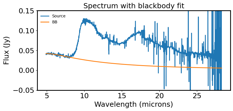
# Plot the spectrum & the model fit to the short wavelength region of the data.
plt.figure(figsize=(8, 4))
plt.plot(spec.spectral_axis, spec.flux, label='Source')
plt.plot(spec.spectral_axis, ybest, label='BB')
plt.xlabel('Wavelength (microns)')
plt.ylabel("Flux ({:latex})".format(spec.flux.unit))
plt.title("Spectrum with blackbody fit")
plt.legend(frameon=False, fontsize='medium')
plt.tight_layout()
plt.ylim(-0.05, 0.15)
plt.show()
plt.close()
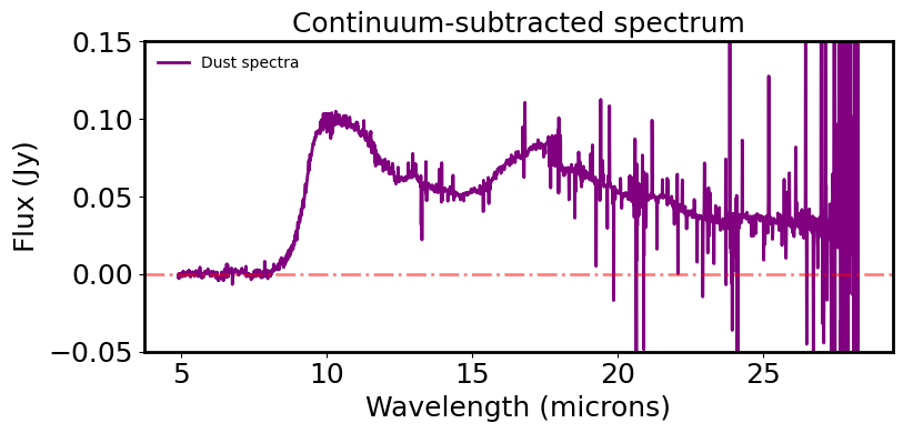
# Now subtract the BB and plot the underlying dust continuum
plt.figure(figsize=(8, 4))
plt.plot(spec.spectral_axis, spec.flux.value - ybest.value, color='purple', label='Dust spectra')
plt.axhline(0, color='r', linestyle='dashdot', alpha=0.5)
plt.xlabel('Wavelength (microns)')
plt.ylabel("Flux ({:latex})".format(spec.flux.unit))
plt.title("Continuum-subtracted spectrum")
plt.legend(frameon=False, fontsize='medium')
plt.tight_layout()
plt.ylim(-0.05, 0.15)
plt.show()
plt.close()
Now have the dust continuum want to look for features and measure their properties.#
Want to find:
Equivalent width
Equivalent flux
Optical depth
Centroids = wavelength with half the flux on either side
As an example lets focus on the amorphous silicate 10 micron region.#
Method - used repeatedly
Fit a spline to the photosphere continuum subtracted spectra excluding the feature in this fit.
Trim the spectra to that wavelength region as the spline is now a different size to the full wavelength range of the spectra.
Make a continuum subtracted and and continuum normalised spectra.
Convert the units of the flux from Jy to W/m^2/wavelength for nice units post line integration.
Determine the feature line flux in units of W/m^2 and the feature centroid. Use continuum subtracted spectra.
Determine the feature equivalent width. Use continuum normalised spectra.
Make sure errors have been propagated correctly.
Store these results in a table
Several molecular and dust features are normally present in the spectra. Repeat for each feature.
Note This seems like a long winded way to do this. Is there a simpler approach?
For instance a tool that takes four wavelengths, fits a line using the data from lam0 to lam1 and lam2 to lam3, then passes the continuum-subtracted spectrum for line integration from lam1 to lam2 with error propagation is needed several times for dust features. But with the current spectra1d framework this takes many steps to write manually and is beyond tedious after doing this for 2 features let alone 20+. Similar framework is also needed for the integrated line centroid with uncertainty, and the extracted equivalent width.
# Subtract the continuum and plot in a new instance of specviz
bbsub_spectra = spec - ybest.value     # continuum subtracted spectra - Dust only
specviz = Specviz()
specviz.show()
specviz.load_data(bbsub_spectra)
Video 6:#
Here is a video that shows how to fit a polynomial to two separate spectral regions within a single subset to remove more underlying continuum
# Video showing how to fit a polynomial to two separate spectral regions within a single subset
HTML('<iframe width="700" height="500" src="https://data.science.stsci.edu/redirect/JWST/jwst-data_analysis_tools/MRS_Mstar_analysis/poly_fit.mov" frameborder="0" allowfullscreen></iframe>')
spectra = specviz.get_spectra()

a = checkKey(spectra, "PolyFit")
if a is True:
    # Extract polynomial fit from Specviz
    poly = spectra["PolyFit"]
else:
    print("No Polyfit")
    fn = download_file('https://data.science.stsci.edu/redirect/JWST/jwst-data_analysis_tools/MRS_Mstar_analysis/poly.fits', cache=True)
    poly = Spectrum1D.read(fn)
Not present
No Polyfit
# Delete any existing output in current directory
if os.path.exists("poly.fits"):
    os.remove("poly.fits")
else:
    print("The poly.fits file does not exist")
The poly.fits file does not exist
# Save if you so desire. Keep commented otherwise.
# poly.write('poly.fits')
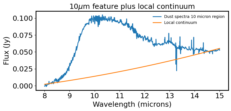
# Fit a local continuum between the flux densities at: 8.0 - 8.1 & 14.9 - 15.0 microns
# (i.e. excluding the line itself)
sw_region = 8.0 # lam0
sw_line = 8.1 # lam1
lw_line = 14.9 # lam2
lw_region = 15.0 # lam3
# Zoom in on the line complex & extract
line_reg_10 = SpectralRegion([(sw_region*u.um, lw_region*u.um)])
line_spec = extract_region(bbsub_spectra, line_reg_10)
polysub = extract_region(poly, line_reg_10)
line_y_continuum = polysub.flux
# -----------------------------------------------------------------
# Generate a continuum subtracted and continuum normalised spectra
line_spec_norm = Spectrum1D(spectral_axis=line_spec.spectral_axis, flux=line_spec.flux/line_y_continuum, uncertainty=StdDevUncertainty(np.zeros(len(line_spec.spectral_axis))))
line_spec_consub = Spectrum1D(spectral_axis=line_spec.spectral_axis, flux=line_spec.flux - line_y_continuum, uncertainty=StdDevUncertainty(np.zeros(len(line_spec.spectral_axis))))
# -----------------------------------------------------------------
# Plot the dust feature & continuum fit to the region
plt.figure(figsize=(8, 4))
plt.plot(line_spec.spectral_axis, line_spec.flux.value,
label='Dust spectra 10 micron region')
plt.plot(line_spec.spectral_axis, line_y_continuum, label='Local continuum')
plt.xlabel('Wavelength (microns)')
plt.ylabel("Flux ({:latex})".format(spec.flux.unit))
plt.title(r"10$\mu$m feature plus local continuum")
plt.legend(frameon=False, fontsize='medium')
plt.tight_layout()
plt.show()
plt.close()
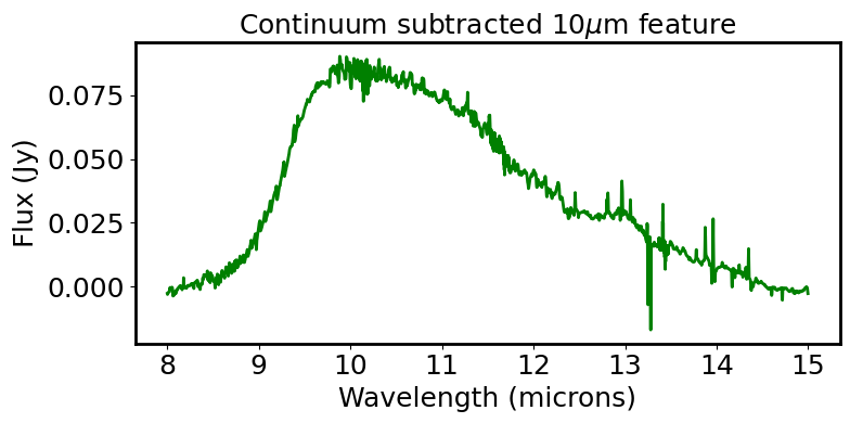
# -----------------------------------------------------------------
# Plot the continuum subtracted 10 micron feature
plt.figure(figsize=(8, 4))
plt.plot(line_spec.spectral_axis, line_spec_consub.flux, color='green',
label='continuum subtracted')
plt.xlabel('Wavelength (microns)')
plt.ylabel("Flux ({:latex})".format(spec.flux.unit))
plt.title(r"Continuum subtracted 10$\mu$m feature")
plt.tight_layout()
plt.show()
plt.close()
# Load 10 um feature back into specviz and calculate the Line flux; Line Centroid; Equivalent width
specviz = Specviz()
specviz.show()
specviz.load_data(line_spec_consub, data_label='Continuum Subtraction')
specviz.load_data(line_spec_norm, data_label='Normalized')
Video7:#
Here is a video that shows how to make line analysis measurements within specviz (i.e., line flux, line centroid, equivalent width)
Note: You want to calculate your equivalent width on the normalized spectrum
Note: You can also hack to convert the line flux value into more conventional units
# Video showing how to measure lines within specviz
HTML('<iframe width="700" height="500" src="https://data.science.stsci.edu/redirect/JWST/jwst-data_analysis_tools/MRS_Mstar_analysis/line_analysis_plugin.mov" frameborder="0" allowfullscreen></iframe>')
# Alternative method to analyze the 10um line within the notebook. Calculate the Line flux; Line Centroid; Equivalent width

line_centroid = centroid(line_spec_consub, SpectralRegion(sw_line*u.um, lw_line*u.um))
line_flux_val = line_flux(line_spec_consub, SpectralRegion(sw_line*u.um, lw_line*u.um))

equivalent_width_val = equivalent_width(line_spec_norm)

# Hack to convert the line flux value into more conventional units
# Necessary as spectra has mixed units: f_nu+lambda
line_flux_val = (line_flux_val * u.micron).to(u.W * u.m**-2 * u.micron,
                                              u.spectral_density(line_centroid)) / u.micron

print("Line_centroid: {:.6} ".format(line_centroid))
print("Integrated line_flux: {:.6} ".format(line_flux_val))
print("Equivalent width: {:.6} ".format(equivalent_width_val))
Line_centroid: 10.7569 micron
Integrated line_flux: 6.65227e-15 W / m2
Equivalent width: -15.0066 micron
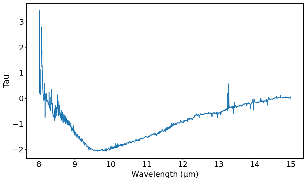
# Compute the optical depth of the 10 micron feature

tau = -(np.log(line_spec.flux.value / line_y_continuum.value))
optdepth_spec = Spectrum1D(spectral_axis=line_spec.spectral_axis,
                           flux=tau*(u.Jy/u.Jy))
# Plot the optical depth of the 10 micron region vs wavelength
plt.figure(figsize=(10, 6))
plt.plot(optdepth_spec.spectral_axis, optdepth_spec.flux)
plt.xlabel("Wavelength ({:latex})".format(spec.spectral_axis.unit))
plt.ylabel('Tau')
plt.tight_layout()
plt.show()
plt.close()
Note At this point repeat all the steps above to isolate solid-state features e.g. for the forsterite feature at at approx 13.3 microns.
This is the end of the notebook that shows some basic analysis of a MIRI MRS spectrum using Cubeviz and Specviz. Much more analysis is possible.
Additional Resources#
About this notebook#
Author: Olivia Jones, Project Scientist, UK ATC.
Updated On: 2020-08-11
Updated On: 2021-09-06 by B. Sargent, STScI Scientist, Space Telescope Science Institute (added MRS Simulated Data)
Updated On: 2021-12-12 by O. Fox, STScI Scientist (added blackbody and polynomial fitting within the notebook)
Top of Page