Cross-Filter PSF Matching#
Use case: Measure galaxy photometry in an extragalactic “blank” field. Related to JDox Science Use Case #22.
Data: JWST simulated NIRCam images from JADES JWST GTO extragalactic blank field.
(Williams et al. 2018) https://ui.adsabs.harvard.edu/abs/2018ApJS..236…33W.
Tools: photutils, matplotlib.
Cross-intrument: potentially NIRISS, MIRI.
Documentation: This notebook is part of a STScI’s larger post-pipeline Data Analysis Tools Ecosystem.
Introduction#
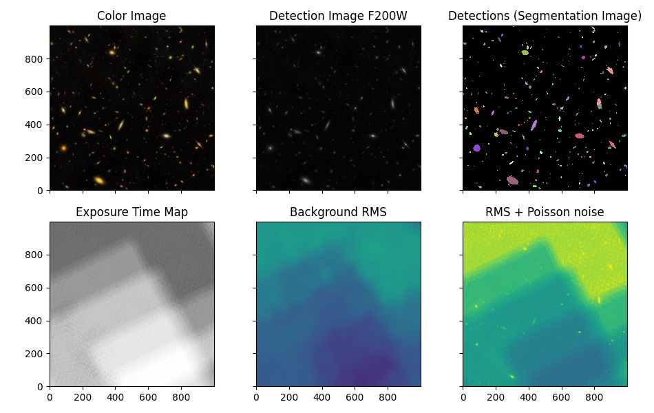
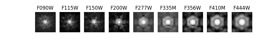
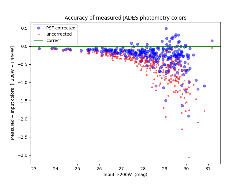
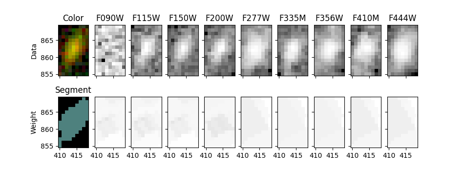
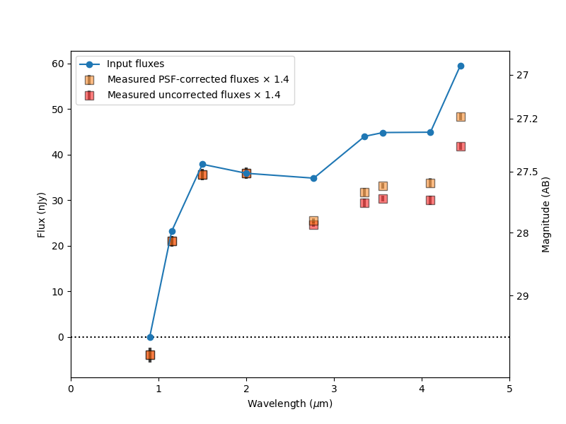
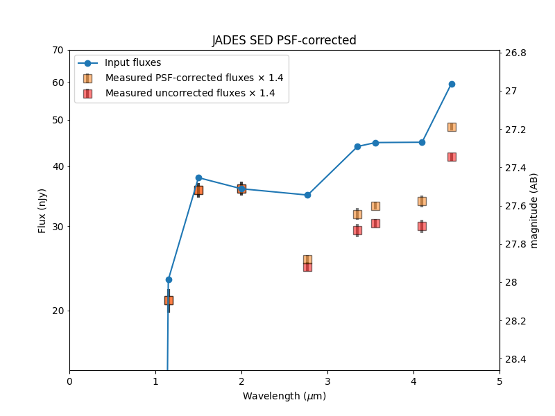
This notebook uses photutils to detect objects/galaxies in NIRCam deep imaging. Detections are first made in a F200W image, then isophotal photometry is obtained in all 9 filters (F090W, F115W, F150W, F200W, F277W, F335M, F356W, F410M, F444W). PSF-matching is used to correct photometry measured in the Long Wavelength images (redder than F200W).
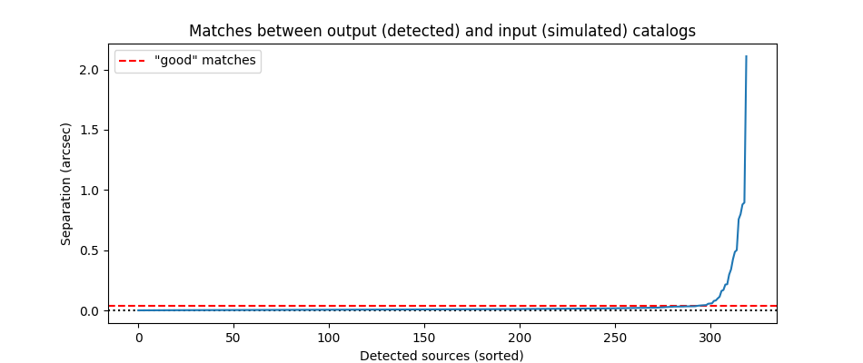
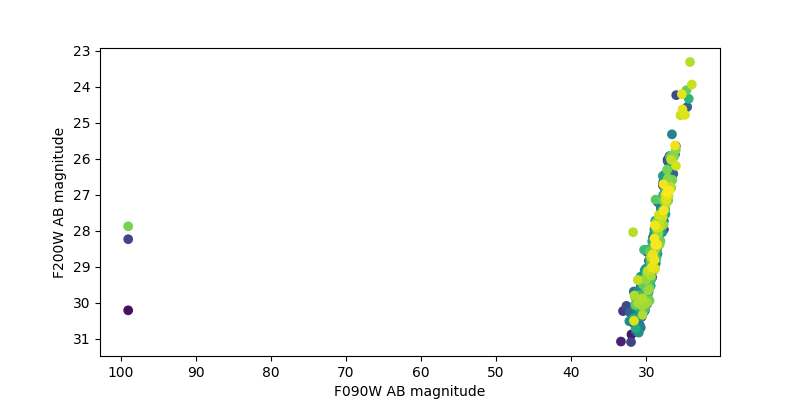
After saving the photometry catalog, the notebook demonstrates how one would load the notebook in a new session. It demonstrates some simple analysis of the full catalog and on an individual galaxy. By comparing the measured colors to simulated input colors, it shows the measurements are more accurate after PSF corrections, though they could be improved further.
The notebook analyzes only the central 1000 x 1000 pixels (30” x 30”) of the full JADES simulation. These cutouts have been staged at STScI with permission from the authors (Williams et al.).
NOTES:
This is a work in progress. More accurate photometry may be obtainable.
These JADES images are simulated using Guitarra, not MIRAGE. They have different properties and units (e-/s) than JWST pipeline products (MJy/sr).
All images are aligned to the same 0.03” pixel grid prior to analysis. This alignment can be done using
reproject, if needed.The flux uncertainty calculations could be improved further by accounting for correlated noise and/or measuring the noise in each image more directly.
Developer’s Note:
Summary of issues reported below:
units work with
plotbut are incompatible witherrorbarandtextflux units can be automatically converted to AB magnitudes, but flux uncertainties cannot be automatically converted to magnitude uncertainties
secondary axis should automatically handle conversion between flux and AB magnitude units
sharexandshareydon’t work with WCSprojection
And I couldn’t figure out how to:
Make plot axes autoscale to only some of plotted data
Make tooltips hover over data points under cursor in interactive plot
# Check PEP 8 style formatting
# %load_ext pycodestyle_magic
# %flake8_on --ignore E261,E501,W291,W2,E302,E305
Import packages#
Numpy for general array computations
Photutils for photometry calculations, PSF matching
Astropy for FITS, WCS, tables, units, color images, plotting, convolution
os and glob for file management
copy for table modfications
Matplotlib for plotting
Watermark to check versions of all imports (optional)
import numpy as np
import os
from glob import glob
from copy import deepcopy

import astropy  # version 4.2 is required to write magnitudes to ecsv file
from astropy.io import fits
import astropy.wcs as wcs
from astropy.table import QTable, Table
import astropy.units as u
from astropy.visualization import make_lupton_rgb, SqrtStretch, LogStretch, hist
from astropy.visualization.mpl_normalize import ImageNormalize
from astropy.convolution import Gaussian2DKernel
from astropy.stats import gaussian_fwhm_to_sigma
from astropy.coordinates import SkyCoord

from photutils.background import Background2D, MedianBackground
from photutils.segmentation import (detect_sources, deblend_sources, SourceCatalog,
                                    make_2dgaussian_kernel, SegmentationImage)
from photutils.utils import calc_total_error

from photutils.psf_matching import SplitCosineBellWindow, make_kernel
from photutils.psf_matching.utils import resize_psf
from astropy.convolution import convolve, convolve_fft # , Gaussian2DKernel, Tophat2DKernel
Matplotlib setup for plotting#
There are two versions
notebook– gives interactive plots, but makes the overall notebook a bit harder to scrollinline– gives non-interactive plots for better overall scrolling
Developer’s Notes:
`%matplotlib notebook` occasionally creates oversized plot; need to rerun cell to get it to settle back down
import matplotlib.pyplot as plt
import matplotlib as mpl

# Use this version for non-interactive plots (easier scrolling of the notebook)
%matplotlib inline

# Use this version if you want interactive plots
# %matplotlib notebook

import matplotlib.ticker as ticker
mpl_colors = plt.rcParams['axes.prop_cycle'].by_key()['color']

# These gymnastics are needed to make the sizes of the figures
# be the same in both the inline and notebook versions
%config InlineBackend.print_figure_kwargs = {'bbox_inches': None}

mpl.rcParams['savefig.dpi'] = 100
mpl.rcParams['figure.dpi'] = 100

import mplcursors  # optional to hover over plotted points and reveal ID number
# Show versions of Python and imported libraries
try:
    import watermark
    %load_ext watermark
    # %watermark -n -v -m -g -iv
    %watermark -iv -v
except ImportError:
    pass
Create list of images to be loaded and analyzed#
All data and weight images must be aligned to the same pixel grid.
(If needed, use reproject to do so.)
input_file_url = 'https://data.science.stsci.edu/redirect/JWST/jwst-data_analysis_tools/nircam_photometry/'

filters = 'F090W F115W F150W F200W F277W F335M F356W F410M F444W'.split()
wavelengths = np.array([int(filt[1:4]) / 100 for filt in filters]) * u.um  # e.g., F115W = 1.15 microns

# Data images [e-/s], unlike JWST pipeline images that will have units [Myr/sr]
image_files = {}
for filt in filters:
    filename = f'jades_jwst_nircam_goods_s_crop_{filt}.fits'
    image_files[filt] = os.path.join(input_file_url, filename)

# Weight images (Inverse Variance Maps; IVM)
weight_files = {}
for filt in filters:
    filename = f'jades_jwst_nircam_goods_s_crop_{filt}_wht.fits'
    weight_files[filt] = os.path.join(input_file_url, filename)
Load detection image: F200W#
detection_filter = filt = 'F200W'
infile = image_files[filt]
hdu = fits.open(infile)
data = hdu[0].data
imwcs = wcs.WCS(hdu[0].header, hdu)

weight = fits.open(weight_files[filt])[0].data
Report image size and field of view#
ny, nx = data.shape
# image_pixel_scale = np.abs(hdu[0].header['CD1_1']) * 3600
image_pixel_scale = wcs.utils.proj_plane_pixel_scales(imwcs)[0]
image_pixel_scale *= imwcs.wcs.cunit[0].to('arcsec')
outline = '%d x %d pixels' % (ny, nx)
outline += ' = %g" x %g"' % (ny * image_pixel_scale, nx * image_pixel_scale)
outline += ' (%.2f" / pixel)' % image_pixel_scale
print(outline)
1000 x 1000 pixels = 30" x 30" (0.03" / pixel)
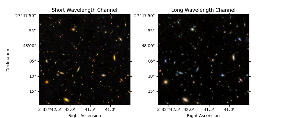
Create color images (optional)#
# 3 NIRCam short wavelength channel images
r = fits.open(image_files['F200W'])[0].data
g = fits.open(image_files['F150W'])[0].data
b = fits.open(image_files['F090W'])[0].data
color_image_short_wavelength = make_lupton_rgb(r, g, b, Q=5, stretch=0.02) # , minimum=-0.001
# 3 NIRCam long wavelength channel images
r = fits.open(image_files['F444W'])[0].data
g = fits.open(image_files['F356W'])[0].data
b = fits.open(image_files['F277W'])[0].data

color_image_long_wavelength = make_lupton_rgb(r, g, b, Q=5, stretch=0.02) # , minimum=-0.001
Developer’s Note:
sharex & sharey appear to have some compatibility issues with projection=imwcs

As a workaround, I tried but was unable to turn off yticklabels in the right plot below
fig = plt.figure(figsize=(9.5, 4))

ax_sw = fig.add_subplot(1, 2, 1, projection=imwcs) # , sharex=True, sharey=True)
ax_sw.imshow(color_image_short_wavelength, origin='lower')
ax_sw.set_xlabel('Right Ascension')
ax_sw.set_ylabel('Declination')
ax_sw.set_title('Short Wavelength Channel')

ax_lw = fig.add_subplot(1, 2, 2, projection=imwcs, sharex=ax_sw, sharey=ax_sw)
ax_lw.imshow(color_image_long_wavelength, origin='lower')
ax_lw.set_xlabel('Right Ascension')
ax_lw.set_title('Long Wavelength Channel')
ax_lw.set_ylabel('')
# ax_lw.set(yticklabels=[])  # this didn't work

# plt.subplots_adjust(left=0.15)
print('Interactive zoom / pan controls both images simultaneously')
Interactive zoom / pan controls both images simultaneously
Detect Sources and Deblend using astropy.photutils#
https://photutils.readthedocs.io/en/latest/segmentation.html
# Define all detection and measurement parameters here so that we do measurements consistently for every image

class Photutils_Catalog:
    def __init__(self, filt, image_file=None, verbose=True):
        self.image_file = image_file or image_files[filt]
        self.hdu = fits.open(self.image_file)
        self.data = self.hdu[0].data
        self.imwcs = wcs.WCS(self.hdu[0].header, self.hdu)
        self.zeropoint = self.hdu[0].header['ABMAG'] * u.ABmag
        self.weight_file = weight_files[filt]
        self.weight = fits.open(weight_files[filt])[0].data
        if verbose:
            print(filt, '  zeropoint =', self.zeropoint)
            print(self.image_file)
            print(self.weight_file)

    def measure_background_map(self, bkg_size=50, filter_size=3, verbose=True):
        # Calculate sigma-clipped background in cells of 50x50 pixels, then median filter over 3x3 cells
        # For best results, the image should span an integer number of cells in both dimensions (here, 1000=20x50 pixels)
        # https://photutils.readthedocs.io/en/stable/background.html
        self.background_map = Background2D(self.data, bkg_size, filter_size=filter_size)

    def run_detect_sources(self, nsigma, npixels, smooth_fwhm=2, kernel_size=5,
                           deblend_levels=32, deblend_contrast=0.001, verbose=True):

        # Set detection threshold map as nsigma times RMS above background pedestal
        detection_threshold = (nsigma * self.background_map.background_rms) + self.background_map.background

        # Before detection, convolve data with Gaussian
        smooth_kernel = make_2dgaussian_kernel(smooth_fwhm, size=kernel_size)
        convolved_data = convolve(self.data, smooth_kernel)

        # Detect sources with npixels connected pixels at/above threshold in data smoothed by kernel
        # https://photutils.readthedocs.io/en/stable/segmentation.html
        self.segm_detect = detect_sources(convolved_data, detection_threshold, n_pixels=npixels)

        # Deblend: separate connected/overlapping sources
        # https://photutils.readthedocs.io/en/stable/segmentation.html#source-deblending
        self.segm_deblend = deblend_sources(convolved_data, self.segm_detect, n_pixels=npixels,
                                            n_levels=deblend_levels, contrast=deblend_contrast)
        if verbose:
            output = 'Cataloged %d objects' % self.segm_deblend.n_labels
            output += ', deblended from %d detections' % self.segm_detect.n_labels
            median_threshold = (nsigma * self.background_map.background_rms_median) \
                + self.background_map.background_median
            output += ' with %d pixels above %g-sigma threshold' % (npixels, nsigma)
            # Background outputs equivalent to those reported by SourceExtractor
            output += '\n'
            output += 'Background median %g' % self.background_map.background_median
            output += ', RMS %g' % self.background_map.background_rms_median
            output += ', threshold median %g' % median_threshold
            print(output)

    def measure_source_properties(self, exposure_time, local_background_width=24):
        # "effective_gain" = exposure time map (conversion from data rate units to counts)
        # weight = inverse variance map = 1 / sigma_background**2 (without sources)
        # https://photutils.readthedocs.io/en/latest/api/photutils.utils.calc_total_error.html
        self.exposure_time_map = exposure_time * self.background_map.background_rms_median**2 * self.weight

        # Data RMS uncertainty is combination of background RMS and source Poisson uncertainties
        background_rms = 1 / np.sqrt(self.weight)
        # effective gain parameter required to be positive everywhere (not zero), so adding small value 1e-8
        self.data_rms = calc_total_error(self.data, background_rms, self.exposure_time_map+1e-8)

        self.catalog = SourceCatalog(self.data-self.background_map.background, self.segm_deblend, wcs=self.imwcs,
                                         error=self.data_rms, background=self.background_map.background,
                                         local_bkg_width=local_background_width)
detection_catalog = Photutils_Catalog(detection_filter)
detection_catalog.measure_background_map()
detection_catalog.run_detect_sources(nsigma=2, npixels=5)
F200W   zeropoint = 27.9973 mag(AB)
https://data.science.stsci.edu/redirect/JWST/jwst-data_analysis_tools/nircam_photometry/jades_jwst_nircam_goods_s_crop_F200W.fits
https://data.science.stsci.edu/redirect/JWST/jwst-data_analysis_tools/nircam_photometry/jades_jwst_nircam_goods_s_crop_F200W_wht.fits
 Background median 6.25759e-06, RMS 0.00187681, threshold median 0.00375987