BOTS Time Series Observations#
Use case: Bright Object Time Series; extracting exoplanet spectra.
Data: JWST simulated NIRSpec data from ground-based campaign; GJ436b spectra from the Goyal et al. (2018).
Tools: scikit, lmfit, scipy, matplotlip, astropy, pandas.
Cross-intrument: .
Documentation: This notebook is part of a STScI’s larger post-pipeline Data Analysis Tools Ecosystem.
Author: David K. Sing (dsing@jhu.edu)
Last updated: 2 July 2020
Introduction#
This notebook uses time series JWST NIRSpec data taken during a ground-based campaign to illustrate extracting exoplanet spectra from time-series observations.
The data are derived from the ISIM-CV3, the cryovacuum campaign of the JWST Integrated Science Instrument Module (ISIM), that took place at Goddard Space Flight Center during the winter 2015-2016 (Kimble et al. 2016). The data can be found at https://www.cosmos.esa.int/web/jwst-nirspec/test-data, and detailed and insightful report of the data by G. Giardino, S. Birkmann, P. Ferruit, B. Dorner, B. Rauscher can be found here: ftp://ftp.cosmos.esa.int/jwstlib/ReleasedCV3dataTimeSeries/CV3_TimeSeries_PRM.tgz
This NIRSpec time series dataset has had a transit light curve injected at the pixel-level, which closely mimics a bright object time series (BOTS) observation of a transiting exoplanet. In this case, a GJ436b spectra from the Goyal et al. (2018) exoplanet grid was selected (clear atmosphere at solar metallicity). With an actual NIRSpec dataset, the noise properties of the detector, jitter, and the effects on extracting exoplanet spectra from time-series observations can more accurately simulated.
Broadly the aim of this notebook is to work with these time series observations to:
Extract 1D spectra from the 2D spectral images.
Define a time series model to fit to the wavelength dependent transit light curve.
Fit each time series wavelength bin of the 1D spectra, measuring the desired quantity \(R_{pl}(\lambda)/R_{star}\).
Produce a measured transmission spectrum that can then be compared to models.
The example outputs the fit light curves for each spectral bin, along with fitting statistics.
Load packages#
This notebook uses packages (matplotlib, astropy, scipy, glob, lmfit, pickle, os, sklearn) which can all be installed in a standard fashion through pip.
Several routines to calculate limb-darkening and a transit model were extracted from ExoTiC-ISm (Laginja & Wakeford 2020 ; https://github.com/hrwakeford/ExoTiC-ISM), and slightly adapted. The full set of stellar models used for the limb-darkening calculation can also be downloaded from ExoTiC-ISM, as this notebook only downloads and loads the single stellar model used to generate the limb darkening.
import numpy as np
import matplotlib.pyplot as plt
import matplotlib.ticker as ticker
from matplotlib.backends.backend_pdf import PdfPages
from astropy.utils.data import download_file
from astropy.table import Table
from astropy.io import fits, ascii
from astropy.modeling.models import custom_model
from astropy.modeling.fitting import LevMarLSQFitter
from scipy.interpolate import interp1d, splev, splrep
from scipy.io import readsav
from scipy import stats
import glob
import lmfit
import pickle
from os import path, mkdir
from sklearn.linear_model import LinearRegression
import pandas as pd
import os
import shutil
Setup Parameters#
Parameters of the fit include directories where the data and limb darkening stellar models are held, along with properties of the planet and star. The stellar and planet values that have been entered here (modeled after GJ436) are the same as was used to model the injected transit. Note, the 4500K stellar model used to inject the transit was hotter than GJ436A.
# SETUP  ----------------------------------------------
# Setup directories
save_directory = './notebookrun2/'          # Local directory to save files to
data_directory = './'                       # Local data to work with fits files if desired

# Setup Detector Properties & Rednoise measurement timescale
gain = 1.0   # 2D spectra has already converted to counts, gain of detector is 1.0
binmeasure = 256   # Binning technique to measure rednoise, choose bin size to evaluate sigma_r
number_of_images = 8192  # Number of images in the dataset

# Setup Planet Properties
grating = 'NIRSpecPrism'
ld_model = '3D'      # 3D/1D stellar model choice (transit was injected with the 3D model)

# Setup Stellar Properties for Limb-Darkening Calculation
Teff = 4500           # Effective Temperature (K)
logg = 4.5            # Surface Gravity
M_H = 0.0            # Stellar Metallicity log_10[M/H]
Rstar = 0.455          # Planet radius (in units of solar radii Run)

# Setup Transit parameters (can get from NASA exoplanet archive)
t0 = 2454865.084034              # bjd time of inferior conjunction
per = 2.64389803                  # orbital period (days) BJD_TDB
rp = 0.0804                      # Planet radius (in units of stellar radii)
a_Rs = 14.54                       # Semi-major axis (input a/Rstar so units of stellar radii)
inc = 86.858 * (2*np.pi/360)      # Orbital inclination (in degrees->radians)
ecc = 0.0                         # Eccentricity
omega = 0.0 * (2*np.pi/360)         # Longitude of periastron (in degrees->radians)

rho_star = (3*np.pi)/(6.67259E-8*(per*86400)**2)*(a_Rs)**3     # Stellar Density (g/cm^3) from a/Rs
# a_Rs=(rho_star*6.67259E-8*per_sec*per_sec/(3*np.pi))**(1/3)  # a/Rs from Stellar Density (g/cm^3)
# Create local directories
if not path.exists(save_directory):
    mkdir(save_directory)      # Create a new directory to save outputs to if needed
if not path.exists(save_directory+'3DGrid'):
    mkdir(save_directory+'3DGrid')      # Create new directory to save
limb_dark_directory = save_directory    # Point to limb darkeing directory contaning 3DGrid/ directory
Download and Load NIRSpec data#
The fits images are loaded, and information including the image date and science spectra are saved.
A default flux offset value BZERO is also taken from the header and subtracted from every science frame.
Reading in the 2^13 fits files is slow. To speed things up, we created a pickle file of the for first instance the fits images are loaded. This 1GB pickle file is loaded instead of reading the fits files if found.
Alternatively, the fits files can be downloaded here: https://data.science.stsci.edu/redirect/JWST/jwst-data_analysis_tools/transit_spectroscopy_notebook/Archive.Trace_SLIT_A_1600_SRAD-PRM-PS-6007102143_37803_JLAB88_injected.tar.gz. The images are in a tar.gz archvie, which needs to be un-archived and data_directory variable set to the directory in the SETUP cell above.
The cell below downloads the 1GB JWST data pickle file, and several other files needed.
# Download 1GB NIRSpec Data
fn_jw = save_directory+'jwst_data.pickle'
if not path.exists(fn_jw):
    fn = download_file('https://data.science.stsci.edu/redirect/JWST/jwst-data_analysis_tools/transit_spectroscopy_notebook/jwst_data.pickle')
    dest = shutil.move(fn, save_directory+'jwst_data.pickle')
    print('JWST Data Download Complete')

# Download further files needed, move to local directory for easier repeated access
fn_sens = download_file('https://data.science.stsci.edu/redirect/JWST/jwst-data_analysis_tools/transit_spectroscopy_notebook/NIRSpec.prism.sensitivity.sav')
dest = shutil.move(fn_sens, save_directory+'NIRSpec.prism.sensitivity.sav')  # Move files to save_directory

fn_ld = download_file('https://data.science.stsci.edu/redirect/JWST/jwst-data_analysis_tools/transit_spectroscopy_notebook/3DGrid/mmu_t45g45m00v05.flx')
destld = shutil.move(fn_ld, save_directory+'3DGrid/mmu_t45g45m00v05.flx')
JWST Data Download Complete
Loads the Pickle File data. Alternatly, the data can be read from the original fits files.
if path.exists(fn_jw):
    dbfile = open(fn_jw, 'rb') # for reading also binary mode is important
    jwst_data = pickle.load(dbfile)
    print('Loading JWST data from Pickle File')
    bjd = jwst_data['bjd']
    wsdata_all = jwst_data['wsdata_all']
    shx = jwst_data['shx']
    shy = jwst_data['shy']
    common_mode = jwst_data['common_mode']
    all_spec = jwst_data['all_spec']
    exposure_length = jwst_data['exposure_length']
    dbfile.close()
    print('Done')
elif not path.exists(fn_jw):
    # Load all fits images
    # Arrays created for BJD time, and the white light curve total_counts
    list = glob.glob(data_directory+"*.fits")
    index_of_images = np.arange(number_of_images)
    bjd = np.zeros((number_of_images))
    exposure_length = np.zeros((number_of_images))
    all_spec = np.zeros((32, 512, number_of_images))
    for i in index_of_images:
        img = list[i]
        print(img)
        hdul = fits.open(img)
        # hdul.info()
        bjd_image = hdul[0].header['BJD_TDB']
        BZERO = hdul[0].header['BZERO']        # flux value offset
        bjd[i] = bjd_image
        expleng = hdul[0].header['INTTIME']    # Total integration time for one MULTIACCUM (seconds)
        exposure_length[i] = expleng/86400.    # Total integration time for one MULTIACCUM (days)
        print(bjd[i])
        data = hdul[0].data
        # total counts in image
        # total_counts[i]=gain*np.sum(data[11:18,170:200]-BZERO) # total counts in 12 pix wide aperture around pixel 60 image
        all_spec[:, :, i] = gain * (data-BZERO)     # Load all spectra into an array subtract flux value offset
        hdul.close()
    # Sort data
    srt = np.argsort(bjd) # index to sort
    bjd = bjd[srt]
    # total_counts=total_counts[srt]
    exposure_length = exposure_length[srt]
    all_spec[:, :, :] = all_spec[:, :, srt]

    # Get Wavelength of Data
    file_wave = download_file('https://data.science.stsci.edu/redirect/JWST/jwst-data_analysis_tools/transit_spectroscopy_notebook/JWST_NIRSpec_wavelength_microns.txt')
    f = open(file_wave, 'r')
    wsdata_all = np.genfromtxt(f)

    print('wsdata size :', wsdata_all.shape)
    print('Data wavelength Loaded :', wsdata_all)
    print('wsdata new size :', wsdata_all.shape)

    # Read in Detrending parameters
    # Mean of parameter must be 0.0 to be properly normalized
    # Idealy standard deviation of parameter = 1.0
    file_xy = download_file('https://data.science.stsci.edu/redirect/JWST/jwst-data_analysis_tools/transit_spectroscopy_notebook/JWST_NIRSpec_Xposs_Yposs_CM_detrending.txt')
    f = open(file_xy, 'r')
    data = np.genfromtxt(f, delimiter=',')
    shx = data[:, 0]
    shy = data[:, 1]
    common_mode = data[:, 2]

    # Store Data in a pickle file
    jwst_data = {'bjd': bjd, 'wsdata_all': wsdata_all, 'shx': shx, 'shy': shy, 'common_mode': common_mode, 'all_spec': all_spec, 'exposure_length': exposure_length}
    dbfile = open('jwst_data.pickle', 'ab') # Its important to use binary mode
    pickle.dump(jwst_data, dbfile)
    dbfile.close()
Loading JWST data from Pickle File
Done
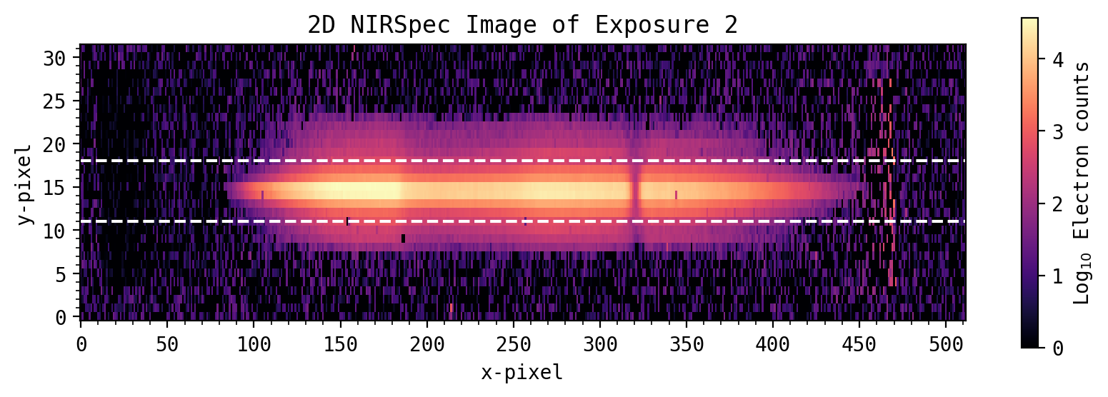
Visualizing the 2D spectral data#
expnum = 2                                           # Choose Exposure number to view

plt.rcParams['figure.figsize'] = [10.0, 3.0]           # Figure dimensions
plt.rcParams['figure.dpi'] = 200                   # Resolution
plt.rcParams['savefig.dpi'] = 200
plt.rcParams['image.aspect'] = 5                     # Aspect ratio (the CCD is quite long!!!)
plt.cmap = plt.cm.magma
plt.cmap.set_bad('k', 1.)
plt.rcParams['image.cmap'] = 'magma'                   # Colormap
plt.rcParams['image.interpolation'] = 'none'
plt.rcParams['image.origin'] = 'lower'
plt.rcParams['font.family'] = "monospace"
plt.rcParams['font.monospace'] = 'DejaVu Sans Mono'

img = all_spec[:, :, expnum]
zeros = np.where(img <= 0)     # Plot on a log scale, so set zero or negative values to a small number
img[zeros] = 1E-10
fig, axs = plt.subplots()
f = axs.imshow(np.log10(img), vmin=0) # Plot image
plt.xlabel('x-pixel')
plt.ylabel('y-pixel')
axs.yaxis.set_major_locator(ticker.MultipleLocator(5))
axs.yaxis.set_minor_locator(ticker.MultipleLocator(1))
axs.xaxis.set_major_locator(ticker.MultipleLocator(50))
axs.xaxis.set_minor_locator(ticker.MultipleLocator(10))
plt.title('2D NIRSpec Image of Exposure ' + str(expnum))
fig.colorbar(f, label='Log$_{10}$ Electron counts', ax=axs)
plt.show()

Extract 1D spectra from 2D array of images#
Ideally, extracting 1D spectra from the 2D images would use optimal aperture extraction along a fit trace with routines equivalent to IRAF/apall. This functionality is not yet available in astro-py.
Several processing steps have already been applied. The 2D spectra here have been flat field corrected, and 1/f noise has been removed from each pixel by subtracting the median count rate from the un-illuminated pixels along each column (see Giardino et al. for more information about 1/f noise). Each 2D image has also been aligned in the X and Y directions, such that each pixel corresponds to the same wavelength. As the CV3 test had no requirements for flux stability, the ~1% flux variations from the LED have also been removed.
For spectral extraction, the example here simply uses a simple summed box. The 8192 2D spectra have been pre-loaded into a numpy array. The spectra peaks at pixel Y=16. For each column, an aperature sum is taken over Y-axis pixels 11 to 18, which contains most of the spectrum counts. Wider aperture would add more counts, but also introduces more noise.
Further cleaning steps are not done here
Ideally, the pixels flagged as bad for various reasons should be cleaned.
Cosmic rays should be identified and removed.
all_spec.shape
y_lower = 11                                             # Lower extraction aperture
y_upper = 18                                             # Upper extraction aperture
all_spec_1D = np.sum(all_spec[y_lower:y_upper, :, :], axis=0) # Sum along Y-axis from pixels 11 to 18
# Plot

plt.rcParams['figure.figsize'] = [10.0, 3.0]           # Figure dimensions
plt.rcParams['figure.dpi'] = 200                   # Resolution
plt.rcParams['savefig.dpi'] = 200
plt.rcParams['image.aspect'] = 5                     # Aspect ratio (the CCD is quite long!!!)
plt.cmap = plt.cm.magma
plt.cmap.set_bad('k', 1.)
plt.rcParams['image.cmap'] = 'magma'                   # Colormap
plt.rcParams['image.interpolation'] = 'none'
plt.rcParams['image.origin'] = 'lower'
plt.rcParams['font.family'] = "monospace"
plt.rcParams['font.monospace'] = 'DejaVu Sans Mono'

img = all_spec[:, :, expnum]
zeros = np.where(img <= 0)     # Plot on a log scale, so set zero or negative values to a small number
img[zeros] = 1E-10
fig, axs = plt.subplots()
f = axs.imshow(np.log10(img), vmin=0)  # Plot image
plt.xlabel('x-pixel')
plt.ylabel('y-pixel')
axs.yaxis.set_major_locator(ticker.MultipleLocator(5))
axs.yaxis.set_minor_locator(ticker.MultipleLocator(1))
axs.xaxis.set_major_locator(ticker.MultipleLocator(50))
axs.xaxis.set_minor_locator(ticker.MultipleLocator(10))
plt.axhline(y_lower, color='w', ls='dashed')
plt.axhline(y_upper, color='w', ls='dashed')
plt.title('2D NIRSpec Image of Exposure '+str(expnum))
fig.colorbar(f, label='Log$_{10}$ Electron counts', ax=axs)
plt.show()
Visualizing the 1D spectral data#
fig, axs = plt.subplots()
f = plt.plot(wsdata_all, all_spec_1D[:, 0], linewidth=2, zorder=0)  # overplot Transit model at data
plt.xlabel(r'Wavelength ($\mu$m)')
plt.ylabel('Flux (e-)')
axs.xaxis.set_major_locator(ticker.MultipleLocator(0.5))
axs.xaxis.set_minor_locator(ticker.MultipleLocator(0.1))
plt.annotate('H$_2$O', xy=(3.0, 42000))
plt.annotate('CO$_2$', xy=(4.2, 42000))
plt.show()
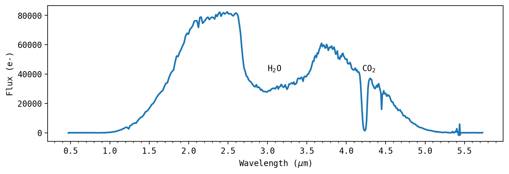
The CV3 test observed a lamp with a similar PSF as JWST will have, and has significant counts from about 1.5 to 4.5 \(\mu\)m.
The cryogenic test chamber had CO\(_2\) and H\(_2\)O ice buildup on the window, which can be seen as spectral absorption features in the 2D spectra.
Calculate Orbital Phase and a separate fine grid model used for plotting purposes#
# Calculate Orbital Phase
phase = (bjd-t0) / (per)  # phase in days relative to T0 ephemeris
phase = phase - np.fix(phase[number_of_images-1]) # Have current phase occur at value 0.0

t_fine = np.linspace(np.min(bjd), np.max(bjd), 1000) # times at which to calculate light curve
phase_fine = (t_fine-t0)/(per)  # phase in days relative to T0 ephemeris
phase_fine = phase_fine-np.fix(phase[number_of_images-1]) # Have current phase occur at value 0.0

b0 = a_Rs * np.sqrt((np.sin(phase * 2 * np.pi)) ** 2 + (np.cos(inc) * np.cos(phase * 2 * np.pi)) ** 2)
intransit = (b0-rp < 1.0E0).nonzero()  # Select indicies between first and fourth contact
outtransit = (b0-rp > 1.0E0).nonzero() # Select indicies out of transit
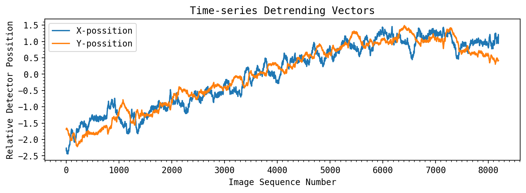
Dealing with Systematic Drift On the Detector#
The CV3 test assessed the stability of the instrument by introducing a large spatial jitter and drift. This resulted in a significant X,Y movement of the spectra on the 2D detector. While this bulk shift has been removed which aligns the spectra, intra- and inter- pixel sensitivities introduce flux variations which need to be removed. The jitter from the CV3 test was more than 30 mas, which is ~4X larger than the JWST stability requirement. Thus, in orbit these detector effects are expected to be significantly smaller, but they will still be present and will need to be modeled and removed from time series observations.
The detector X, Y positions here were measured from cross-correlation of the 2D images (collapsing the spectra along one dimension first), and are saved in arrays \(shx\) and \(shy\). These detending vectors would ideally be measured using the trace position values from the spectral extraction of each integration, as that could also accurately measure integration-to-integration how the spectra spatially changed on the detector.
The detector shifts have original amplitudes near 0.2 pixels, though the vectors have had initial normalization. For detrending purposes, these arrays should have a mean of 0 and standard deviation of 1.0.
A residual color-dependent trend with the LED lamp can also been seen in the CV3 data, which can be partly removed by scaling original common-mode lamp trend, which was measured using the CV3 white light curve.
shx_tmp = shx / np.mean(shx) - 1.0E0       # Set Mean around 0.0
shx_detrend = shx_tmp/np.std(shx_tmp)  # Set standard deviation to 1.0
shy_tmp = shy / np.mean(shy) - 1.0E0       # Set Mean around 0.0
shy_detrend = shy_tmp/np.std(shy_tmp)  # Set standard deviation to 1.0

cm = common_mode / np.mean(common_mode) - 1.0E0
cm_detrend = cm/np.std(cm)

fig, axs = plt.subplots()
plt.plot(shx_detrend, label='X-possition')
plt.plot(shy_detrend, label='Y-possition')
plt.xlabel('Image Sequence Number')
plt.ylabel('Relative Detector Possition')
plt.title('Time-series Detrending Vectors')
axs.xaxis.set_major_locator(ticker.MultipleLocator(1000))
axs.xaxis.set_minor_locator(ticker.MultipleLocator(100))
axs.yaxis.set_major_locator(ticker.MultipleLocator(0.5))
axs.yaxis.set_minor_locator(ticker.MultipleLocator(0.1))
plt.legend()
plt.show()
Create arrays of the vectors used for detrending.#
From Sing et al. 2019: Systematic errors are often removed by a parameterized deterministic model, where the non-transit photometric trends are found to correlate with a number \(n\) of external parameters (or optical state vectors, \(X\)). These parameters describe changes in the instrument or other external factors as a function of time during the observations, and are fit with a coefficient for each optical state parameter, \(p_n\), to model and remove (or detrend) the photometric light curves.
When including systematic trends, the total parameterized model of the flux measurements over time, \(f(t)\), can be modeled as a combination of the theoretical transit model, \(T(t,\theta)\) (which depends upon the transit parameters \(\theta\)), the total baseline flux detected from the star, \(F_0\), and the systematics error model \(S(x)\) giving,
\(f(t) = T(t,\theta)\times F_0 \times S(x)\).
We will use a linear model for the instrument systematic effects.
\(S(x)= p_1 x + p_2 y + p_3 x^2 + p_4 y^2 + p_5 x y + p_6 cm + p_7 \phi \)
\(cm\) is the common_mode trend, and \(\phi\) is a linear time trend which helps remove changing H\(_2\)O ice within the H\(_2\)O spectral feature.
shx = shx_detrend
shy = shy_detrend
common_mode = cm_detrend

XX = np.array([shx, shy, shx**2, shy**2, shx*shy, common_mode, np.ones(number_of_images)])  # Detrending array without linear time trend
XX = np.transpose(XX)
XXX = np.array([shx, shy, shx**2, shy**2, shx*shy, common_mode, phase, np.ones(number_of_images)])  # Detrending array with with linear time trend
XXX = np.transpose(XXX)
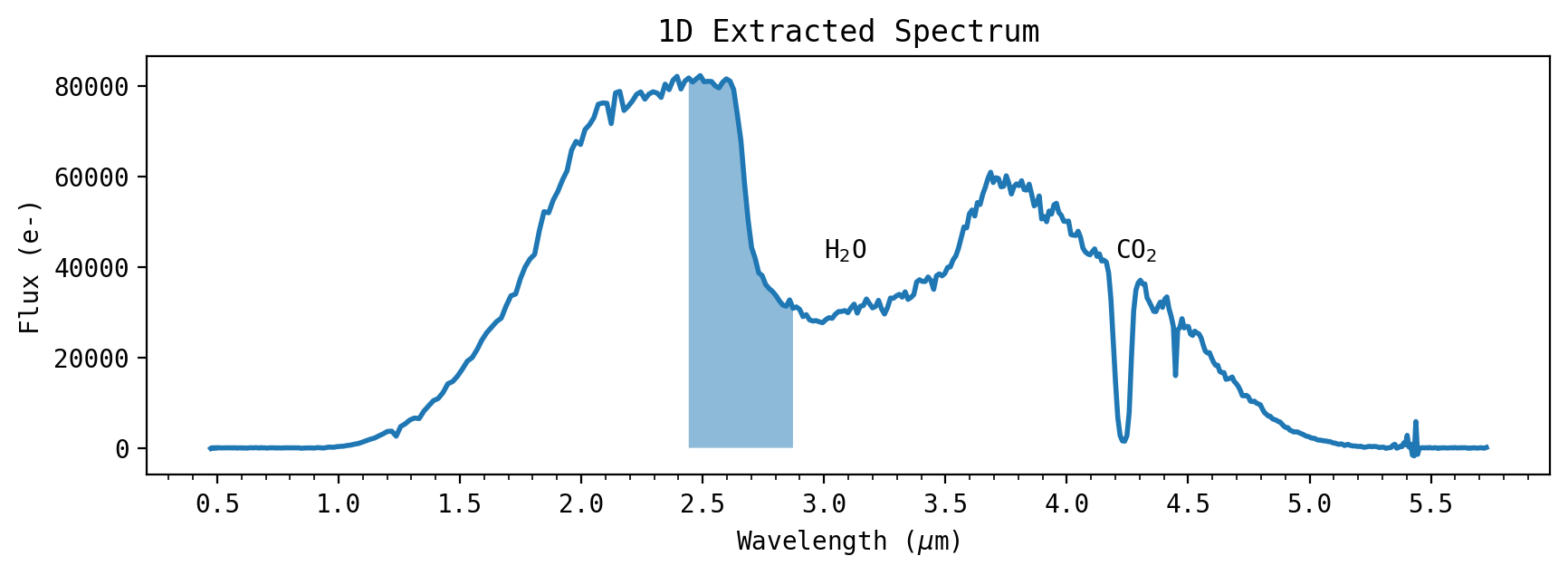
Linear Regression can be used to quickly determine the parameters \(p_n\) using the out-of-transit data.
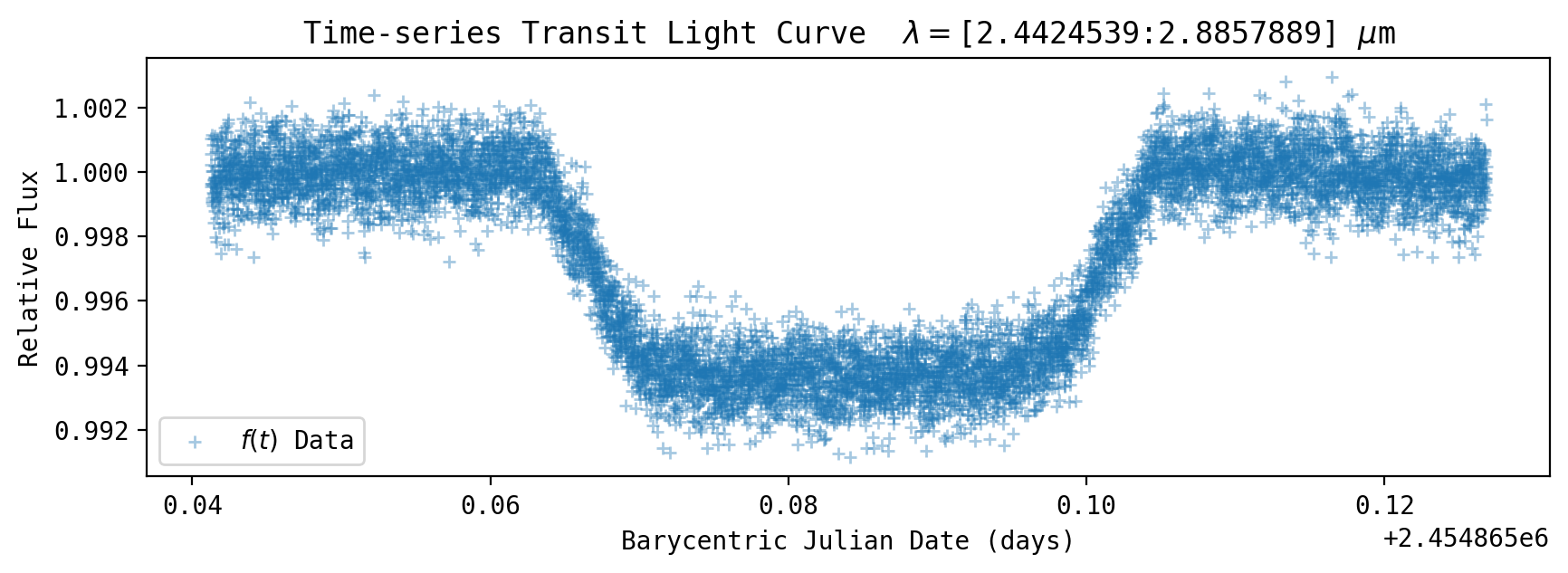
Here, we take a wavelength bin of the data (pixels 170 to 200) to make a time series. The out-of-transit points are selected and a linear regression of \(S(x)\) is done to determine the optical state parameters \(p_n\)
pix1 = 170       # wavelength bin lower range
pix2 = 200       # wavelength bin upper range
y = np.sum(all_spec_1D[pix1:pix2, :], axis=0)    # flux over a selected wavelength bin

msize = plt.rcParams['lines.markersize'] ** 2.           # default marker size
plt.rcParams['figure.figsize'] = [10.0, 3.0]           # Figure dimensions

fig, axs = plt.subplots()
f = plt.plot(wsdata_all, all_spec_1D[:, 0], linewidth=2, zorder=0)  # Plot Region of wavelength bin
plt.fill_between(wsdata_all[pix1:pix2], 0, all_spec_1D[pix1:pix2, 0], alpha=0.5)
plt.xlabel(r'Wavelength ($\mu$m)')
plt.ylabel('Flux (e-)')
plt.title('1D Extracted Spectrum')
axs.xaxis.set_major_locator(ticker.MultipleLocator(0.5))
axs.xaxis.set_minor_locator(ticker.MultipleLocator(0.1))
plt.annotate('H$_2$O', xy=(3.0, 42000))
plt.annotate('CO$_2$', xy=(4.2, 42000))
plt.show()

fig, axs = plt.subplots()
plt.scatter(bjd, y/np.mean(y[outtransit]), label='$f(t)$ Data', zorder=1, s=msize*0.75, linewidth=1, alpha=0.4, marker='+', edgecolors='blue')
plt.xlabel('Barycentric Julian Date (days)')
plt.ylabel('Relative Flux')
plt.title(r'Time-series Transit Light Curve  $\lambda=$['+str(wsdata_all[pix1])+':'+str(wsdata_all[pix2]) + r'] $\mu$m')
plt.legend()
plt.show()

regressor = LinearRegression()
regressor.fit(XX[outtransit], y[outtransit]/np.mean(y[outtransit]))
print('Linear Regression Coefficients:')
print(regressor.coef_)
/tmp/ipykernel_2145/1502773371.py:21: UserWarning: You passed a edgecolor/edgecolors ('blue') for an unfilled marker ('+').  Matplotlib is ignoring the edgecolor in favor of the facecolor.  This behavior may change in the future.
  plt.scatter(bjd, y/np.mean(y[outtransit]), label='$f(t)$ Data', zorder=1, s=msize*0.75, linewidth=1, alpha=0.4, marker='+', edgecolors='blue')
Linear Regression Coefficients:
[ 2.35589645e-04  2.33200386e-04 -1.43527088e-04 -4.65560797e-05
  1.94065907e-04 -4.51855007e-04  0.00000000e+00]
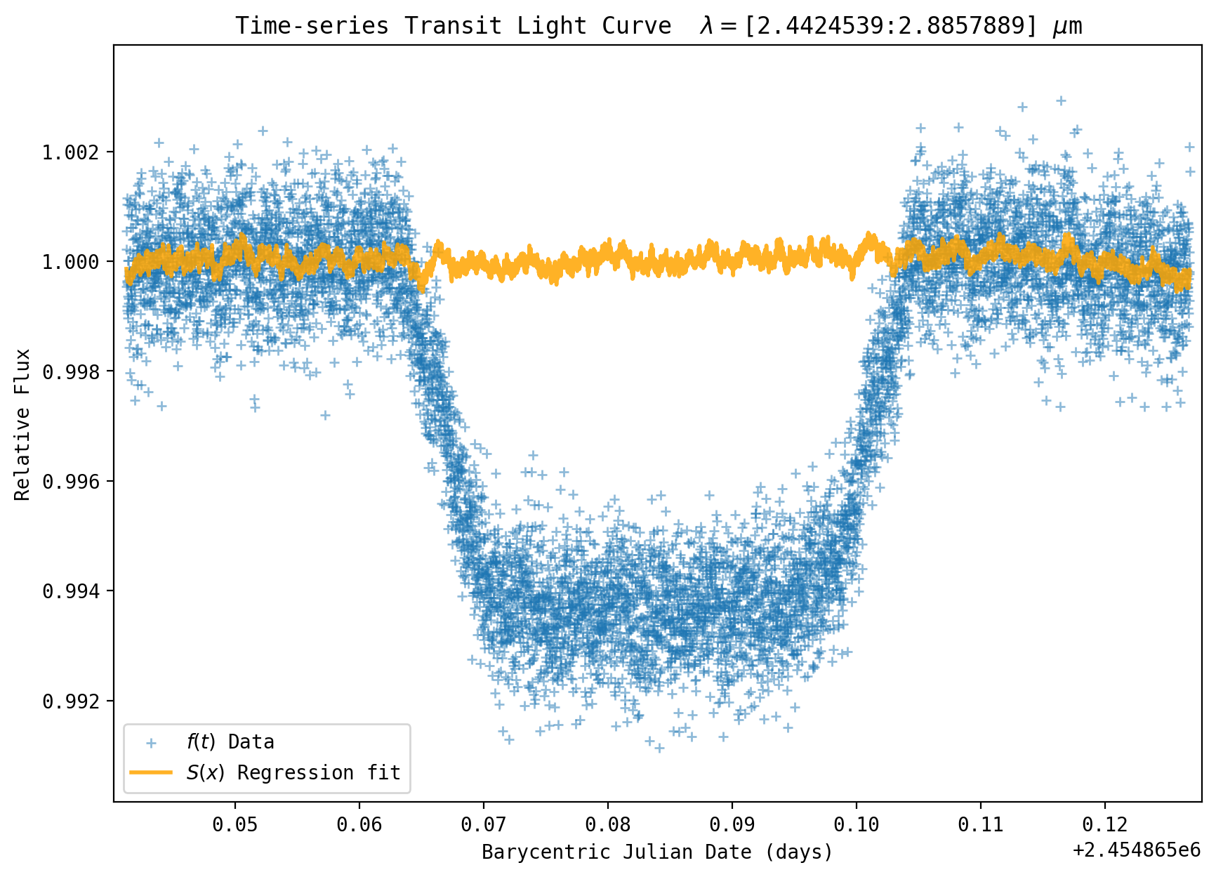
The coefficients are on the order of ~10\(^{-4}\) so the trends have an amplitude on the order of 100’s of ppm.
Visualize the fit
yfit = regressor.predict(XX)                         # Project the fit over the whole time series

plt.rcParams['figure.figsize'] = [10.0, 7.0]           # Figure dimensions
msize = plt.rcParams['lines.markersize'] ** 2.           # default marker size
plt.scatter(bjd, y/np.mean(y[outtransit]), label='$f(t)$ Data', zorder=1, s=msize*0.75, linewidth=1, alpha=0.5, marker='+', edgecolors='blue')
f = plt.plot(bjd, yfit, label='$S(x)$ Regression fit ', linewidth=2, color='orange', zorder=2, alpha=0.85)
plt.xlabel('Barycentric Julian Date (days)')
plt.ylabel('Relative Flux')
plt.title(r'Time-series Transit Light Curve  $\lambda=$['+str(wsdata_all[pix1])+':'+str(wsdata_all[pix2]) + r'] $\mu$m')
axs.xaxis.set_major_locator(ticker.MultipleLocator(0.01))
axs.xaxis.set_minor_locator(ticker.MultipleLocator(0.005))
axs.yaxis.set_major_locator(ticker.MultipleLocator(0.002))
axs.yaxis.set_minor_locator(ticker.MultipleLocator(0.001))
yplot = y / np.mean(y[outtransit])
plt.ylim(yplot.min() * 0.999, yplot.max()*1.001)
plt.xlim(bjd.min()-0.001, bjd.max()+0.001)
plt.legend(loc='lower left')
plt.show()
/tmp/ipykernel_2145/3911644354.py:5: UserWarning: You passed a edgecolor/edgecolors ('blue') for an unfilled marker ('+').  Matplotlib is ignoring the edgecolor in favor of the facecolor.  This behavior may change in the future.
  plt.scatter(bjd, y/np.mean(y[outtransit]), label='$f(t)$ Data', zorder=1, s=msize*0.75, linewidth=1, alpha=0.5, marker='+', edgecolors='blue')
Transit and Limb-Darkening Model Functions#
Define a functions used by the fitting routines. These which will take the transit and systematic parameters and create our full transit light curve model
\(model = T(t,\theta)\times F_0 \times S(x)\)
compares it to the data
\(y = f(t)\)
by returning the residuals
\((y-model)/(\sigma_y)\)
To calculate the transit model, here we use Mandel and Agol (2002) as coded in python by H. Wakeford (ExoTiC-ISM).
To calculate the stellar limb-darkening, we use the procedure from Sing et al. (2010) which uses stellar models and fits for non-linear limb darkening coefficients, with a module as coded in python by H. Wakeford (ExoTiC-ISM).
A new orbit is first calculated based on the system parameters of \(a/R_{star}\), the cosine of the inclination \(cos(i)\), and the orbital phase \(\phi\). The inputs are the orbit distance between the planet-star center \(b\) at each phase, limb-darkening parameters (\(c_1,c_2,c_3,c_4\)), and the planet-to-star radius ratio \(R_p/R_{star}\).
@custom_model
def nonlinear_limb_darkening(x, c0=0.0, c1=0.0, c2=0.0, c3=0.0):
    """
    Define non-linear limb darkening model with four parameters c0, c1, c2, c3.
    """
    model = (1. - (c0 * (1. - x ** (1. / 2)) + c1 * (1. - x ** (2. / 2)) + c2 * (1. - x ** (3. / 2)) + c3 *
                   (1. - x ** (4. / 2))))
    return model


@custom_model
def quadratic_limb_darkening(x, aLD=0.0, bLD=0.0):
    """
    Define linear limb darkening model with parameters aLD and bLD.
    """
    model = 1. - aLD * (1. - x) - bLD * (1. - x) ** (4. / 2.)
    return model


def limb_dark_fit(grating, wsdata, M_H, Teff, logg, dirsen, ld_model='1D'):
    """
    Calculates stellar limb-darkening coefficients for a given wavelength bin.

    Currently supports:
    HST STIS G750L, G750M, G430L gratings
    HST WFC3 UVIS/G280, IR/G102, IR/G141 grisms

    What is used for 1D models - Kurucz (?)
    Procedure from Sing et al. (2010, A&A, 510, A21).
    Uses 3D limb darkening from Magic et al. (2015, A&A, 573, 90).
    Uses photon FLUX Sum over (lambda*dlamba).
    :param grating: string; grating to use ('G430L','G750L','G750M', 'G280', 'G102', 'G141')
    :param wsdata: array; data wavelength solution
    :param M_H: float; stellar metallicity
    :param Teff: float; stellar effective temperature (K)
    :param logg: float; stellar gravity
    :param dirsen: string; path to main limb darkening directory
    :param ld_model: string; '1D' or '3D', makes choice between limb darkening models; default is 1D
    :return: uLD: float; linear limb darkening coefficient
    aLD, bLD: float; quadratic limb darkening coefficients
    cp1, cp2, cp3, cp4: float; three-parameter limb darkening coefficients
    c1, c2, c3, c4: float; non-linear limb-darkening coefficients
    """

    print('You are using the', str(ld_model), 'limb darkening models.')

    if ld_model == '1D':

        direc = os.path.join(dirsen, 'Kurucz')

        print('Current Directories Entered:')
        print('  ' + dirsen)
        print('  ' + direc)

        # Select metallicity
        M_H_Grid = np.array([-0.1, -0.2, -0.3, -0.5, -1.0, -1.5, -2.0, -2.5, -3.0, -3.5, -4.0, -4.5, -5.0, 0.0, 0.1, 0.2, 0.3, 0.5, 1.0])
        M_H_Grid_load = np.array([0, 1, 2, 3, 5, 7, 8, 9, 10, 11, 12, 13, 14, 17, 20, 21, 22, 23, 24])
        optM = (abs(M_H - M_H_Grid)).argmin()
        MH_ind = M_H_Grid_load[optM]

        # Determine which model is to be used, by using the input metallicity M_H to figure out the file name we need
        direc = 'Kurucz'
        file_list = 'kuruczlist.sav'
        sav1 = readsav(os.path.join(dirsen, file_list))
        model = bytes.decode(sav1['li'][MH_ind])  # Convert object of type "byte" to "string"

        # Select Teff and subsequently logg
        Teff_Grid = np.array([3500, 3750, 4000, 4250, 4500, 4750, 5000, 5250, 5500, 5750, 6000, 6250, 6500])
        optT = (abs(Teff - Teff_Grid)).argmin()

        logg_Grid = np.array([4.0, 4.5, 5.0])
        optG = (abs(logg - logg_Grid)).argmin()

        if logg_Grid[optG] == 4.0:
            Teff_Grid_load = np.array([8, 19, 30, 41, 52, 63, 74, 85, 96, 107, 118, 129, 138])

        elif logg_Grid[optG] == 4.5:
            Teff_Grid_load = np.array([9, 20, 31, 42, 53, 64, 75, 86, 97, 108, 119, 129, 139])

        elif logg_Grid[optG] == 5.0:
            Teff_Grid_load = np.array([10, 21, 32, 43, 54, 65, 76, 87, 98, 109, 120, 130, 140])

        # Where in the model file is the section for the Teff we want? Index T_ind tells us that.
        T_ind = Teff_Grid_load[optT]
        header_rows = 3    # How many rows in each section we ignore for the data reading
        data_rows = 1221   # How  many rows of data we read
        line_skip_data = (T_ind + 1) * header_rows + T_ind * data_rows   # Calculate how many lines in the model file we need to skip in order to get to the part we need (for the Teff we want).
        line_skip_header = T_ind * (data_rows + header_rows)

        # Read the header, in case we want to have the actual Teff, logg and M_H info.
        # headerinfo is a pandas object.
        headerinfo = pd.read_csv(os.path.join(dirsen, direc, model), delim_whitespace=True, header=None,
                                 skiprows=line_skip_header, nrows=1)

        Teff_model = headerinfo[1].values[0]
        logg_model = headerinfo[3].values[0]
        MH_model = headerinfo[6].values[0]
        MH_model = float(MH_model[1:-1])

        print('\nClosest values to your inputs:')
        print('Teff: ', Teff_model)
        print('M_H: ', MH_model)
        print('log(g): ', logg_model)

        # Read the data; data is a pandas object.
        data = pd.read_csv(os.path.join(dirsen, direc, model), delim_whitespace=True, header=None,
                           skiprows=line_skip_data, nrows=data_rows)

        # Unpack the data
        ws = data[0].values * 10   # Import wavelength data
        f0 = data[1].values / (ws * ws)
        f1 = data[2].values * f0 / 100000.
        f2 = data[3].values * f0 / 100000.
        f3 = data[4].values * f0 / 100000.
        f4 = data[5].values * f0 / 100000.
        f5 = data[6].values * f0 / 100000.
        f6 = data[7].values * f0 / 100000.
        f7 = data[8].values * f0 / 100000.
        f8 = data[9].values * f0 / 100000.
        f9 = data[10].values * f0 / 100000.
        f10 = data[11].values * f0 / 100000.
        f11 = data[12].values * f0 / 100000.
        f12 = data[13].values * f0 / 100000.
        f13 = data[14].values * f0 / 100000.
        f14 = data[15].values * f0 / 100000.
        f15 = data[16].values * f0 / 100000.
        f16 = data[17].values * f0 / 100000.

        # Make single big array of them
        fcalc = np.array([f0, f1, f2, f3, f4, f5, f6, f7, f8, f9, f10, f11, f12, f13, f14, f15, f16])
        phot1 = np.zeros(fcalc.shape[0])

        # Define mu
        mu = np.array([1.000, .900, .800, .700, .600, .500, .400, .300, .250, .200, .150, .125, .100, .075, .050, .025, .010])

        # Passed on to main body of function are: ws, fcalc, phot1, mu

    elif ld_model == '3D':

        direc = os.path.join(dirsen, '3DGrid')

        print('Current Directories Entered:')
        print('  ' + dirsen)
        print('  ' + direc)

        # Select metallicity
        M_H_Grid = np.array([-3.0, -2.0, -1.0, 0.0])  # Available metallicity values in 3D models
        M_H_Grid_load = ['30', '20', '10', '00']  # The according identifiers to individual available M_H values
        optM = (abs(M_H - M_H_Grid)).argmin()  # Find index at which the closes M_H values from available values is to the input M_H.

        # Select Teff
        Teff_Grid = np.array([4000, 4500, 5000, 5500, 5777, 6000, 6500, 7000])  # Available Teff values in 3D models
        optT = (abs(Teff - Teff_Grid)).argmin()  # Find index at which the Teff values is, that is closest to input Teff.

        # Select logg, depending on Teff. If several logg possibilities are given for one Teff, pick the one that is
        # closest to user input (logg).

        if Teff_Grid[optT] == 4000:
            logg_Grid = np.array([1.5, 2.0, 2.5])
            optG = (abs(logg - logg_Grid)).argmin()

        elif Teff_Grid[optT] == 4500:
            logg_Grid = np.array([2.0, 2.5, 3.0, 3.5, 4.0, 4.5, 5.0])
            optG = (abs(logg - logg_Grid)).argmin()

        elif Teff_Grid[optT] == 5000:
            logg_Grid = np.array([2.0, 2.5, 3.0, 3.5, 4.0, 4.5, 5.0])
            optG = (abs(logg - logg_Grid)).argmin()

        elif Teff_Grid[optT] == 5500:
            logg_Grid = np.array([3.0, 3.5, 4.0, 4.5, 5.0])
            optG = (abs(logg - logg_Grid)).argmin()

        elif Teff_Grid[optT] == 5777:
            logg_Grid = np.array([4.4])
            optG = 0

        elif Teff_Grid[optT] == 6000:
            logg_Grid = np.array([3.5, 4.0, 4.5])
            optG = (abs(logg - logg_Grid)).argmin()

        elif Teff_Grid[optT] == 6500:
            logg_Grid = np.array([4.0, 4.5])
            optG = (abs(logg - logg_Grid)).argmin()

        elif Teff_Grid[optT] == 7000:
            logg_Grid = np.array([4.5])
            optG = 0

        # Select Teff and Log g. Mtxt, Ttxt and Gtxt are then put together as string to load correct files.
        Mtxt = M_H_Grid_load[optM]
        Ttxt = "{:2.0f}".format(Teff_Grid[optT] / 100)
        if Teff_Grid[optT] == 5777:
            Ttxt = "{:4.0f}".format(Teff_Grid[optT])
        Gtxt = "{:2.0f}".format(logg_Grid[optG] * 10)

        #
        file = 'mmu_t' + Ttxt + 'g' + Gtxt + 'm' + Mtxt + 'v05.flx'
        print('Filename:', file)

        # Read data from IDL .sav file
        sav = readsav(os.path.join(direc, file))  # readsav reads an IDL .sav file
        ws = sav['mmd'].lam[0]  # read in wavelength
        flux = sav['mmd'].flx  # read in flux
        Teff_model = Teff_Grid[optT]
        logg_model = logg_Grid[optG]
        MH_model = str(M_H_Grid[optM])

        print('\nClosest values to your inputs:')
        print('Teff  : ', Teff_model)
        print('M_H   : ', MH_model)
        print('log(g): ', logg_model)

        f0 = flux[0]
        f1 = flux[1]
        f2 = flux[2]
        f3 = flux[3]
        f4 = flux[4]
        f5 = flux[5]
        f6 = flux[6]
        f7 = flux[7]
        f8 = flux[8]
        f9 = flux[9]
        f10 = flux[10]

        # Make single big array of them
        fcalc = np.array([f0, f1, f2, f3, f4, f5, f6, f7, f8, f9, f10])
        phot1 = np.zeros(fcalc.shape[0])

        # Mu from grid
        # 0.00000    0.0100000    0.0500000     0.100000     0.200000     0.300000   0.500000     0.700000     0.800000     0.900000      1.00000
        mu = sav['mmd'].mu

        # Passed on to main body of function are: ws, fcalc, phot1, mu

    # Load response function and interpolate onto kurucz model grid

    # FOR STIS
    if grating == 'G430L':
        sav = readsav(os.path.join(dirsen, 'G430L.STIS.sensitivity.sav'))  # wssens,sensitivity
        wssens = sav['wssens']
        sensitivity = sav['sensitivity']
        wdel = 3

    if grating == 'G750M':
        sav = readsav(os.path.join(dirsen, 'G750M.STIS.sensitivity.sav'))  # wssens, sensitivity
        wssens = sav['wssens']
        sensitivity = sav['sensitivity']
        wdel = 0.554

    if grating == 'G750L':
        sav = readsav(os.path.join(dirsen, 'G750L.STIS.sensitivity.sav'))  # wssens, sensitivity
        wssens = sav['wssens']
        sensitivity = sav['sensitivity']
        wdel = 4.882

    # FOR WFC3
    if grating == 'G141':  # http://www.stsci.edu/hst/acs/analysis/reference_files/synphot_tables.html
        sav = readsav(os.path.join(dirsen, 'G141.WFC3.sensitivity.sav'))  # wssens, sensitivity
        wssens = sav['wssens']
        sensitivity = sav['sensitivity']
        wdel = 1

    if grating == 'G102':  # http://www.stsci.edu/hst/acs/analysis/reference_files/synphot_tables.html
        sav = readsav(os.path.join(dirsen, 'G141.WFC3.sensitivity.sav'))  # wssens, sensitivity
        wssens = sav['wssens']
        sensitivity = sav['sensitivity']
        wdel = 1

    if grating == 'G280':  # http://www.stsci.edu/hst/acs/analysis/reference_files/synphot_tables.html
        sav = readsav(os.path.join(dirsen, 'G280.WFC3.sensitivity.sav'))  # wssens, sensitivity
        wssens = sav['wssens']
        sensitivity = sav['sensitivity']
        wdel = 1

    # FOR JWST
    if grating == 'NIRSpecPrism':  # http://www.stsci.edu/hst/acs/analysis/reference_files/synphot_tables.html
        sav = readsav(os.path.join(dirsen, 'NIRSpec.prism.sensitivity.sav'))  # wssens, sensitivity
        wssens = sav['wssens']
        sensitivity = sav['sensitivity']
        wdel = 12

    widek = np.arange(len(wsdata))
    wsHST = wssens
    wsHST = np.concatenate((np.array([wsHST[0] - wdel - wdel, wsHST[0] - wdel]),
                            wsHST,
                            np.array([wsHST[len(wsHST) - 1] + wdel,
                                      wsHST[len(wsHST) - 1] + wdel + wdel])))

    respoutHST = sensitivity / np.max(sensitivity)
    respoutHST = np.concatenate((np.zeros(2), respoutHST, np.zeros(2)))
    inter_resp = interp1d(wsHST, respoutHST, bounds_error=False, fill_value=0)
    respout = inter_resp(ws)  # interpolate sensitivity curve onto model wavelength grid

    wsdata = np.concatenate((np.array([wsdata[0] - wdel - wdel, wsdata[0] - wdel]), wsdata,
                             np.array([wsdata[len(wsdata) - 1] + wdel, wsdata[len(wsdata) - 1] + wdel + wdel])))
    respwavebin = wsdata / wsdata * 0.0
    widek = widek + 2  # need to add two indicies to compensate for padding with 2 zeros
    respwavebin[widek] = 1.0
    data_resp = interp1d(wsdata, respwavebin, bounds_error=False, fill_value=0)
    reswavebinout = data_resp(ws)  # interpolate data onto model wavelength grid

    # Integrate over the spectra to make synthetic photometric points.
    for i in range(fcalc.shape[0]):  # Loop over spectra at diff angles
        fcal = fcalc[i, :]
        Tot = int_tabulated(ws, ws * respout * reswavebinout)
        phot1[i] = (int_tabulated(ws, ws * respout * reswavebinout * fcal, sort=True)) / Tot

    if ld_model == '1D':
        yall = phot1 / phot1[0]
    elif ld_model == '3D':
        yall = phot1 / phot1[10]

    # Co = np.zeros((6, 4))   # NOT-REUSED

    # A = [0.0, 0.0, 0.0, 0.0]  # c1, c2, c3, c4      # NOT-REUSED
    x = mu[1:]     # wavelength
    y = yall[1:]   # flux
    # weights = x / x   # NOT-REUSED

    # Start fitting the different models
    fitter = LevMarLSQFitter()

    # Fit a four parameter non-linear limb darkening model and get fitted variables, c1, c2, c3, c4.
    corot_4_param = nonlinear_limb_darkening()
    corot_4_param = fitter(corot_4_param, x, y)
    c1, c2, c3, c4 = corot_4_param.parameters

    # Fit a three parameter non-linear limb darkening model and get fitted variables, cp2, cp3, cp4 (cp1 = 0).
    corot_3_param = nonlinear_limb_darkening()
    corot_3_param.c0.fixed = True  # 3 param is just 4 param with c0 = 0.0
    corot_3_param = fitter(corot_3_param, x, y)
    cp1, cp2, cp3, cp4 = corot_3_param.parameters

    # Fit a quadratic limb darkening model and get fitted parameters aLD and bLD.
    quadratic = quadratic_limb_darkening()
    quadratic = fitter(quadratic, x, y)
    aLD, bLD = quadratic.parameters

    # Fit a linear limb darkening model and get fitted variable uLD.
    linear = nonlinear_limb_darkening()
    linear.c0.fixed = True
    linear.c2.fixed = True
    linear.c3.fixed = True
    linear = fitter(linear, x, y)
    uLD = linear.c1.value

    print('\nLimb darkening parameters:')
    print("4param \t{:0.8f}\t{:0.8f}\t{:0.8f}\t{:0.8f}".format(c1, c2, c3, c4))
    print("3param \t{:0.8f}\t{:0.8f}\t{:0.8f}".format(cp2, cp3, cp4))
    print("Quad \t{:0.8f}\t{:0.8f}".format(aLD, bLD))
    print("Linear \t{:0.8f}".format(uLD))

    return uLD, c1, c2, c3, c4, cp1, cp2, cp3, cp4, aLD, bLD


def int_tabulated(X, F, sort=False):
    Xsegments = len(X) - 1

    # Sort vectors into ascending order.
    if not sort:
        ii = np.argsort(X)
        X = X[ii]
        F = F[ii]

    while (Xsegments % 4) != 0:
        Xsegments = Xsegments + 1

    Xmin = np.min(X)
    Xmax = np.max(X)

    # Uniform step size.
    h = (Xmax + 0.0 - Xmin) / Xsegments
    # Compute the interpolates at Xgrid.
    # x values of interpolates >> Xgrid = h * FINDGEN(Xsegments + 1L) + Xmin
    z = splev(h * np.arange(Xsegments + 1) + Xmin, splrep(X, F))

    # Compute the integral using the 5-point Newton-Cotes formula.
    ii = (np.arange((len(z) - 1) / 4, dtype=int) + 1) * 4

    return np.sum(2.0 * h * (7.0 * (z[ii - 4] + z[ii]) + 32.0 * (z[ii - 3] + z[ii - 1]) + 12.0 * z[ii - 2]) / 45.0)
Now define the transit model function#
def occultnl(rl, c1, c2, c3, c4, b0):
    """
    MANDEL & AGOL (2002) transit model.
    :param rl: float, transit depth (Rp/R*)
    :param c1: float, limb darkening parameter 1
    :param c2: float, limb darkening parameter 2
    :param c3: float, limb darkening parameter 3
    :param c4: float, limb darkening parameter 4
    :param b0: impact parameter in stellar radii
    :return: mulimb0: limb-darkened transit model, mulimbf: lightcurves for each component that you put in the model
    """
    mulimb0 = occultuniform(b0, rl)
    bt0 = b0
    fac = np.max(np.abs(mulimb0 - 1))
    if fac == 0:
        fac = 1e-6  # DKS edit

    omega = 4 * ((1 - c1 - c2 - c3 - c4) / 4 + c1 / 5 + c2 / 6 + c3 / 7 + c4 / 8)
    nb = len(b0)
    indx = np.where(mulimb0 != 1.0)[0]
    if len(indx) == 0:
        indx = -1
    mulimb = mulimb0[indx]
    mulimbf = np.zeros((5, nb))
    mulimbf[0, :] = mulimbf[0, :] + 1.
    mulimbf[1, :] = mulimbf[1, :] + 0.8
    mulimbf[2, :] = mulimbf[2, :] + 2 / 3
    mulimbf[3, :] = mulimbf[3, :] + 4 / 7
    mulimbf[4, :] = mulimbf[4, :] + 0.5
    nr = np.int64(2)
    dmumax = 1.0

    while (dmumax > fac * 1.e-3) and (nr <= 131072):
        # print(nr)
        mulimbp = mulimb
        nr = nr * 2
        dt = 0.5 * np.pi / nr
        t = dt * np.arange(nr + 1)
        th = t + 0.5 * dt
        r = np.sin(t)
        sig = np.sqrt(np.cos(th[nr - 1]))
        mulimbhalf = sig ** 3 * mulimb0[indx] / (1 - r[nr - 1])
        mulimb1 = sig ** 4 * mulimb0[indx] / (1 - r[nr - 1])
        mulimb3half = sig ** 5 * mulimb0[indx] / (1 - r[nr - 1])
        mulimb2 = sig ** 6 * mulimb0[indx] / (1 - r[nr - 1])
        for i in range(1, nr):
            mu = occultuniform(b0[indx] / r[i], rl / r[i])
            sig1 = np.sqrt(np.cos(th[i - 1]))
            sig2 = np.sqrt(np.cos(th[i]))
            mulimbhalf = mulimbhalf + r[i] ** 2 * mu * (sig1 ** 3 / (r[i] - r[i - 1]) - sig2 ** 3 / (r[i + 1] - r[i]))
            mulimb1 = mulimb1 + r[i] ** 2 * mu * (sig1 ** 4 / (r[i] - r[i - 1]) - sig2 ** 4 / (r[i + 1] - r[i]))
            mulimb3half = mulimb3half + r[i] ** 2 * mu * (sig1 ** 5 / (r[i] - r[i - 1]) - sig2 ** 5 / (r[i + 1] - r[i]))
            mulimb2 = mulimb2 + r[i] ** 2 * mu * (sig1 ** 6 / (r[i] - r[i - 1]) - sig2 ** 6 / (r[i + 1] - r[i]))

        mulimb = ((1 - c1 - c2 - c3 - c4) * mulimb0[
            indx] + c1 * mulimbhalf * dt + c2 * mulimb1 * dt + c3 * mulimb3half * dt + c4 * mulimb2 * dt) / omega
        ix1 = np.where(mulimb + mulimbp != 0.)[0]
        if len(ix1) == 0:
            ix1 = -1

        # print(ix1)
        # python cannot index on single values so you need to use atlest_1d for the below to work when mulimb is a single value
        dmumax = np.max(np.abs(np.atleast_1d(mulimb)[ix1] - np.atleast_1d(mulimbp)[ix1]) / (
                np.atleast_1d(mulimb)[ix1] + np.atleast_1d(mulimbp)[ix1]))

    mulimbf[0, indx] = np.atleast_1d(mulimb0)[indx]
    mulimbf[1, indx] = mulimbhalf * dt
    mulimbf[2, indx] = mulimb1 * dt
    mulimbf[3, indx] = mulimb3half * dt
    mulimbf[4, indx] = mulimb2 * dt
    np.atleast_1d(mulimb0)[indx] = mulimb
    b0 = bt0

    return mulimb0, mulimbf


def occultuniform(b0, w):
    """
    Compute the lightcurve for occultation of a uniform source without microlensing (Mandel & Agol 2002).

    :param b0: array; impact parameter in units of stellar radii
    :param w: array; occulting star size in units of stellar radius
    :return: muo1: float; fraction of flux at each b0 for a uniform source
    """

    if np.abs(w - 0.5) < 1.0e-3:
        w = 0.5

    nb = len(np.atleast_1d(b0))
    muo1 = np.zeros(nb)

    for i in range(nb):
        # substitute z=b0(i) to shorten expressions
        z = np.atleast_1d(b0)[i]
        # z = z.value    # stripping it of astropy units
        if z >= 1+w:
            muo1[i] = 1.0
            continue

        if w >= 1 and z <= w-1:
            muo1[i] = 0.0
            continue

        if z >= np.abs(1-w) and z <= 1+w:
            kap1 = np.arccos(np.min(np.append((1 - w ** 2 + z ** 2) / 2 / z, 1.)))
            kap0 = np.arccos(np.min(np.append((w ** 2 + z ** 2 - 1) / 2 / w / z, 1.)))
            lambdae = w ** 2 * kap0 + kap1
            lambdae = (lambdae - 0.5 * np.sqrt(np.max(np.append(4. * z ** 2 - (1 + z ** 2 - w ** 2) ** 2, 0.)))) / np.pi
            muo1[i] = 1 - lambdae

        if z <= 1-w:
            muo1[i] = 1 - w ** 2
            continue

    return muo1
Now define the function to generate the transit light curve and compare it to the data#
# Functions to call and calculate models
def residual(p, phase, x, y, err, c1, c2, c3, c4):
    # calculate new orbit
    b0 = p['a_Rs'].value * np.sqrt((np.sin(phase * 2 * np.pi)) ** 2 + (p['cosinc'].value * np.cos(phase * 2 * np.pi)) ** 2)
    # Select indicies between first and fourth contact
    intransit = (b0-p['rprs'].value < 1.0E0).nonzero()
    # Make light curve model, set all values initially to 1.0
    light_curve = b0/b0
    mulimb0, mulimbf = occultnl(p['rprs'].value, c1, c2, c3, c4, b0[intransit])  # Madel and Agol
    light_curve[intransit] = mulimb0
    model = (light_curve) * p['f0'].value * (p['Fslope'].value * phase + p['xsh'].value * shx + p['x2sh'].value * shx**2. + p['ysh'].value * shy + p['y2sh'].value * shy**2. + p['xysh'].value * shy * shx + p['comm'].value * common_mode + 1.0) # transit model is baseline flux X transit model X systematics model
    chi2now = np.sum((y-model)**2/err**2)
    res = np.std((y-model)/p['f0'].value)
    print("rprs: ", p['rprs'].value, "current chi^2=", chi2now, ' scatter ', res, end="\r")
    return (y-model)/err
    # return np.sum((y-model)**2/err**2)
A function is also defined to return just the transit model \(T(t,\theta)\)
def model_fine(p):  # Make Transit model with a fine grid for plotting purposes
    b0 = p['a_Rs'].value * np.sqrt((np.sin(phase_fine * 2 * np.pi)) ** 2 + (p['cosinc'].value * np.cos(phase_fine * 2 * np.pi)) ** 2)
    mulimb0, mulimbf = occultnl(p['rprs'].value, c1, c2, c3, c4, b0)  # Madel and Agol
    model_fine = mulimb0
    return model_fine
Now add a transit model to the Example Light curve. Here, we’ve compute the limb darkening coefficients, then use them in the transit light curve.
wave1 = wsdata_all[pix1]
wave2 = wsdata_all[pix2]
bin_wave_index = ((wsdata_all > wave1) & (wsdata_all <= wave2)).nonzero()
wsdata = wsdata_all[bin_wave_index]*1E4 # Select wavelength bin values (um=> angstroms)

_uLD, c1, c2, c3, c4, _cp1, _cp2, _cp3, _cp4, aLD, bLD = limb_dark_fit(grating, wsdata, M_H, Teff, logg, limb_dark_directory, ld_model)
You are using the 3D limb darkening models.
Current Directories Entered:
  ./notebookrun2/
  ./notebookrun2/3DGrid
Filename: mmu_t45g45m00v05.flx

Closest values to your inputs:
Teff  :  4500
M_H   :  0.0
log(g):  4.5
Limb darkening parameters:
4param 	0.87682038	-0.73755073	0.57722987	-0.19560354
3param 	2.19231523	-3.11195028	1.36536758
Quad 	0.02781793	0.37167807
Linear 	0.34303528
Now run the transit model.
The transit parameters such as inclination and \(a/R_{star}\) have been setup at the beginning of the notebook.
# Run the Transit Model
rl = 0.0825     # Planet-to-star Radius Ratio

b0 = a_Rs * np.sqrt((np.sin(phase * 2 * np.pi)) ** 2 + (np.cos(inc) * np.cos(phase * 2 * np.pi)) ** 2)
intransit = (b0-rl < 1.0E0).nonzero()  # Select indicies between first and fourth contact

mulimb0, mulimbf = occultnl(rl, c1, c2, c3, c4, b0)  # Mandel & Agol non-linear limb darkened transit model
model = mulimb0*yfit

# plot
plt.rcParams['figure.figsize'] = [10.0, 7.0]           # Figure dimensions
msize = plt.rcParams['lines.markersize'] ** 2.           # default marker size
fig = plt.figure(constrained_layout=True)
gs = fig.add_gridspec(3, 1, hspace=0.00, wspace=0.00)
ax1 = fig.add_subplot(gs[0:2, :])
ax1.scatter(bjd, y/np.mean(y[outtransit]), label='$f(t)$ Data', zorder=1, s=msize*0.75, linewidth=1, alpha=0.5, marker='+', edgecolors='blue')
ax1.plot(bjd, model, label='$S(x)$ Regression fit ', linewidth=2, color='orange', zorder=2, alpha=0.85)
ax1.xaxis.set_ticklabels([])
plt.ylabel('Relative Flux')
plt.title(r'Time-series Transit Light Curve  $\lambda=$['+str(wsdata_all[pix1])+':'+str(wsdata_all[pix2]) + r'] $\mu$m')
ax1.xaxis.set_major_locator(ticker.MultipleLocator(0.01))
ax1.xaxis.set_minor_locator(ticker.MultipleLocator(0.005))
ax1.yaxis.set_major_locator(ticker.MultipleLocator(0.002))
ax1.yaxis.set_minor_locator(ticker.MultipleLocator(0.001))
yplot = y/np.mean(y[outtransit])
plt.ylim(yplot.min()*0.999, yplot.max()*1.001)
plt.xlim(bjd.min()-0.001, bjd.max()+0.001)
plt.legend()
fig.add_subplot(ax1)
# Residual
ax2 = fig.add_subplot(gs[2, :])
ax2.scatter(bjd, 1E6*(y/np.mean(y[outtransit])-model), label='$f(t)$ Data', zorder=1, s=msize*0.75, linewidth=1, alpha=0.5, marker='+', edgecolors='blue')
wsb, wsb_bin_edges, binnumber = stats.binned_statistic(bjd, 1E6*(y/np.mean(y[outtransit])-model), bins=256)
plt.scatter(wsb_bin_edges[1:], wsb, linewidth=2, alpha=0.75, facecolors='orange', edgecolors='none', marker='o', zorder=25)
plt.xlabel('Barycentric Julian Date (days)')
plt.ylabel('Residual (ppm)')
ax2.xaxis.set_major_locator(ticker.MultipleLocator(0.01))
ax2.xaxis.set_minor_locator(ticker.MultipleLocator(0.005))
yplot = y / np.mean(y[outtransit])
plt.xlim(bjd.min()-0.001, bjd.max()+0.001)
fig.add_subplot(ax2)
plt.show()

# print chi^2 value
err = np.sqrt(y) / np.mean(y[outtransit])
print('Chi^2 = '+str(np.sum((y/np.mean(y[outtransit])-model)**2/err**2)))

print('Residual Standard Deviation : '+str(1E6*np.std((y/np.mean(y[outtransit])-model)))+' ppm')
print('256 Bin Standard Deviation  :'+str(np.std(wsb))+' ppm')
/tmp/ipykernel_2145/1695522111.py:16: UserWarning: You passed a edgecolor/edgecolors ('blue') for an unfilled marker ('+').  Matplotlib is ignoring the edgecolor in favor of the facecolor.  This behavior may change in the future.
  ax1.scatter(bjd, y/np.mean(y[outtransit]), label='$f(t)$ Data', zorder=1, s=msize*0.75, linewidth=1, alpha=0.5, marker='+', edgecolors='blue')
/tmp/ipykernel_2145/1695522111.py:32: UserWarning: You passed a edgecolor/edgecolors ('blue') for an unfilled marker ('+').  Matplotlib is ignoring the edgecolor in favor of the facecolor.  This behavior may change in the future.
  ax2.scatter(bjd, 1E6*(y/np.mean(y[outtransit])-model), label='$f(t)$ Data', zorder=1, s=msize*0.75, linewidth=1, alpha=0.5, marker='+', edgecolors='blue')
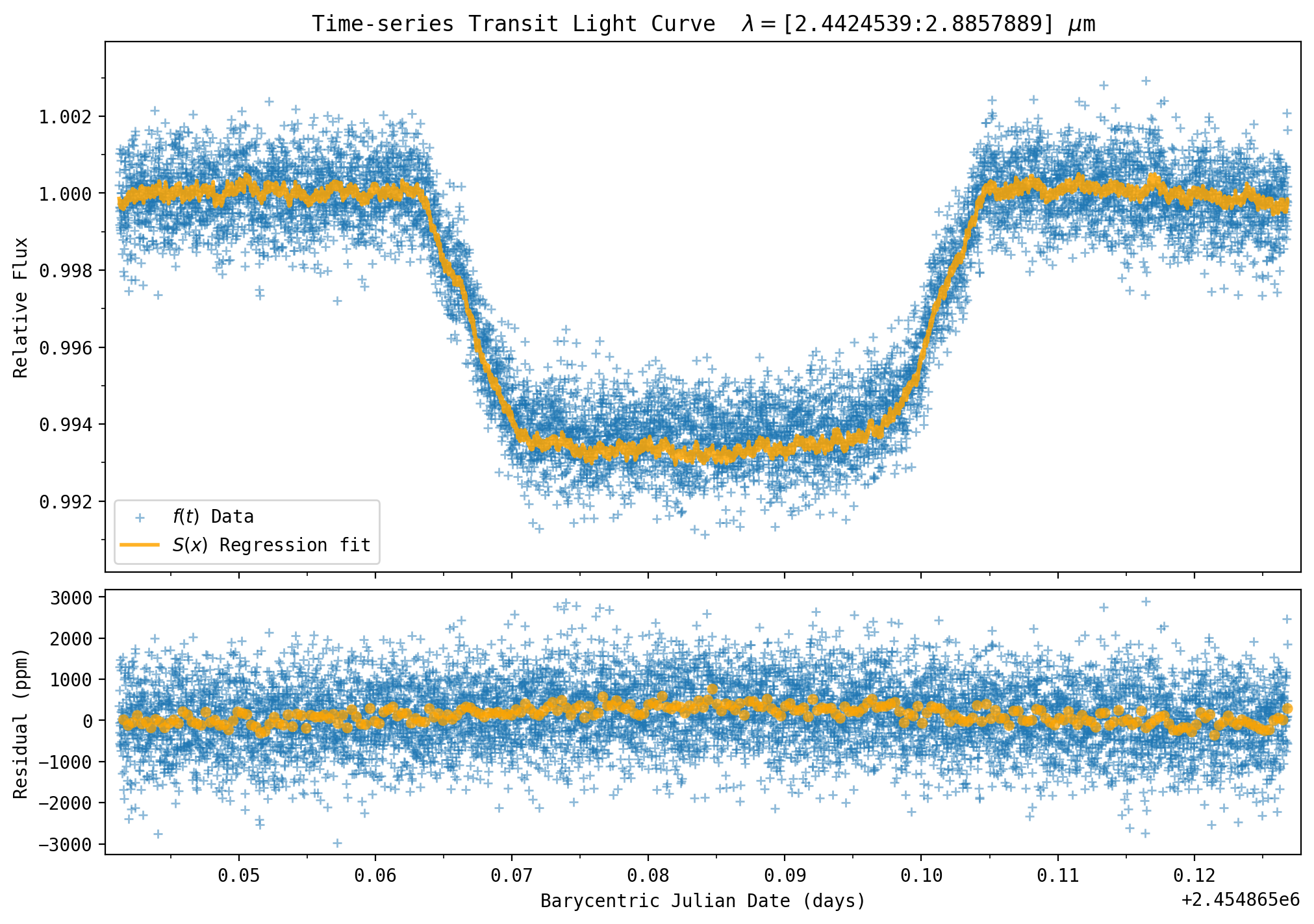
Chi^2 = 9265.443675786024
Residual Standard Deviation : 789.8093551317617 ppm
256 Bin Standard Deviation  :196.83308658203643 ppm
Note that the model transit depth is a little too deep compared to the data. The planet radius needs to be smaller, and the parameter \(rl\) is closer to 0.08. As an exercise you can re-run the above cell changing the planet radius to \(rl\)=0.0805 and compare the \(\chi^2\) value to the previous default value (\(\chi^2\)=9265.4 at \(rl\) = 0.0825).
FIT Transit Light Curves#
Now we can fit each light curve, optimizing the fit parameters with a least-squares fit. Here a Levenberg-Marquart fit is used to find a \(\chi^2\) minimum and estimate uncertainties using the lmfit package (https://lmfit.github.io/lmfit-py/fitting.html).
In practice, first we would fit the white light curve, which consists of summing over all of the wavelengths in the entire 1D spectra. This can then be used to fit for the system parameters such as inclination and transit time, and then the spectroscopic channels are then fixed to these values as they are wavelength-independent. However, the CV3 data required the overall variations of the lamp to be removed, which prevents our use of using this data for a white light curve analysis. Here, we proceed to fitting for the spectroscopic light curve bins.
The steps are as follows:
1) Wavelength Bin is selected

2) Limb-darkening coefficients are calculated from a stellar model for each bin.

3) An initial linear regression is performed on the out-of-transit data to start the
systematic fit parameters, this greatly speeds up the fit as those parameters start
near their global minimum.

4) The fit is started, and some statistics are output during the minimization

5) Once the best-fit is found, a number of statistics are displayed

6) Finally, several plots are generated which are stored as PDFs and the next bin is started.
These steps are performed for each spectral bin.
In this example, the planet radius is set to vary in the fit along with the baseline flux and instrument systematic parameters.
Setup Wavelengths to fit over#
The spectra must be binned in wavelength to get sufficient counts to reach ~100 ppm levels needed. The spectra has significant counts from about pixel 100 to 400, we start at pixel \(k0\) and bin the spectra by \(wk\) pixels.
Several arrays are also defined.
k0 = 113 # 98   #100
kend = 392 # 422
wk = 15
number_of_bins = int((kend-k0)/wk)
wsd = np.zeros((number_of_bins))
werr = np.zeros((number_of_bins))
rprs = np.zeros((number_of_bins))
rerr = np.zeros((number_of_bins))
sig_r = np.zeros((number_of_bins))
sig_w = np.zeros((number_of_bins))
beta = np.zeros((number_of_bins))
depth = np.zeros((number_of_bins))
depth_err = np.zeros((number_of_bins))
Loop Over Wavelength Bins Fitting Each Lightcurve#
Note this step takes considerable time to complete (~20 min, few minutes/bin)#
Each wavelength bin is fit for the transit+systematics model. Various outputs including plots are saved. Can skip to the next cells to load pre-computed results.
k = k0 # wavelength to start
# --------------------------------------------------------------------------
# Loop over wavelength bins and fit for each one
for bin in range(0, number_of_bins):
# Select wavelength bin
wave1 = wsdata_all[k]
wave2 = wsdata_all[k+wk]
# Indicies to select for wavelgth bin
bin_wave_index = ((wsdata_all > wave1) & (wsdata_all <= wave2)).nonzero()
# make light curve bin
wave_bin_counts = np.sum(all_spec_1D[k+1:k+wk, :], axis=0) # Sum Wavelength pixels
wave_bin_counts_err = np.sqrt(wave_bin_counts) # adopt photon noise for errors
# Calculate Limb Darkening
wsdata = wsdata_all[bin_wave_index]*1E4 # Select wavelength bin values (um=> angstroms)
_uLD, c1, c2, c3, c4, _cp1, _cp2, _cp3, _cp4, aLD, bLD = limb_dark_fit(grating, wsdata, M_H, Teff, logg, limb_dark_directory, ld_model)
print('\nc1 = {}'.format(c1))
print('c2 = {}'.format(c2))
print('c3 = {}'.format(c3))
print('c4 = {}'.format(c4))
print('')
# u = [c1,c2,c3,c4] # limb darkening coefficients
# u = [aLD, bLD]
# Make initial model
# Setup LMFIT
x = bjd # X data
y = wave_bin_counts # Y data
err = wave_bin_counts_err # Y Error
# Perform Quick Linear regression on out-of-transit data to obtain accurate starting Detector fit values
if wave1 > 2.7 and wave1 < 3.45:
regressor.fit(XXX[outtransit], y[outtransit]/np.mean(y[outtransit]))
else:
regressor.fit(XX[outtransit], y[outtransit]/np.mean(y[outtransit]))
# create a set of Parameters for LMFIT https://lmfit.github.io/lmfit-py/parameters.html
# class Parameter(name, value=None, vary=True, min=- inf, max=inf, expr=None, brute_step=None, user_data=None)
# Set vary=0 to fix
# Set vary=1 to fit
p = lmfit.Parameters() # object to store L-M fit Parameters # Parameter Name
p.add('cosinc', value=np.cos(inc), vary=0) # inclination, vary cos(inclin)
p.add('rho_star', value=rho_star, vary=0) # stellar density
p.add('a_Rs', value=a_Rs, vary=0) # a/Rstar
p.add('rprs', value=rp, vary=1, min=0, max=1) # planet-to-star radius ratio
p.add('t0', value=t0, vary=0) # Transit T0
p.add('f0', value=np.mean(y[outtransit]), vary=1, min=0) # Baseline Flux
p.add('ecc', value=ecc, vary=0, min=0, max=1) # eccentricity
p.add('omega', value=omega, vary=0) # arguments of periatron
# Turn on a linear slope in water feature to account for presumably changing H2O ice builtup on widow during cryogenic test
if wave1 > 2.7 and wave1 < 3.45:
p.add('Fslope', value=regressor.coef_[6], vary=1) # Orbital phase
else:
p.add('Fslope', value=0, vary=0) # Orbital phase
p.add('xsh', value=regressor.coef_[0], vary=1) # Detector X-shift detrending
p.add('ysh', value=regressor.coef_[1], vary=1) # Detector X-shift detrending
p.add('x2sh', value=regressor.coef_[2], vary=1) # Detector X^2-shift detrending
p.add('y2sh', value=regressor.coef_[3], vary=1) # Detector Y^2-shift detrending
p.add('xysh', value=regressor.coef_[4], vary=1) # Detector X*Y detrending
p.add('comm', value=regressor.coef_[5], vary=1) # Common-Mode detrending
# Perform Minimization https://lmfit.github.io/lmfit-py/fitting.html
# create Minimizer
# mini = lmfit.Minimizer(residual, p, nan_policy='omit',fcn_args=(phase,x,y,err)
print('')
print('Fitting Bin', bin, ' Wavelength =', np.mean(wsdata)/1E4, ' Range= [', wave1, ':', wave2, ']')
# solve with Levenberg-Marquardt using the
result = lmfit.minimize(residual, params=p, args=(phase, x, y, err, c1, c2, c3, c4))
# result = mini.minimize(method='emcee')
print('')
print('Re-Fitting Bin', bin, ' Wavelength =', np.mean(wsdata)/1E4, ' Range= [', wave1, ':', wave2, ']')
# --------------------------------------------------------------------------
print("")
print("redchi", result.redchi)
print("chi2", result.chisqr)
print("nfree", result.nfree)
print("bic", result.bic)
print("aic", result.aic)
print("L-M FIT Variable")
print(lmfit.fit_report(result.params))
text_file = open(save_directory+'JWST_NIRSpec_Prism_fit_light_curve_bin'+str(bin)+'_statistics.txt', "w")
n = text_file.write("\nredchi "+str(result.redchi))
n = text_file.write("\nchi2 "+str(result.chisqr))
n = text_file.write("\nnfree "+str(result.nfree))
n = text_file.write("\nbic "+str(result.bic))
n = text_file.write("\naic "+str(result.aic))
n = text_file.write(lmfit.fit_report(result.params))
# file-output.py
# Update with best-fit parameters
p['rho_star'].value = result.params['rho_star'].value
p['cosinc'].value = result.params['cosinc'].value
p['rprs'].value = result.params['rprs'].value
p['t0'].value = result.params['t0'].value
p['f0'].value = result.params['f0'].value
p['Fslope'].value = result.params['Fslope'].value
p['xsh'].value = result.params['xsh'].value
p['ysh'].value = result.params['ysh'].value
p['x2sh'].value = result.params['x2sh'].value
p['y2sh'].value = result.params['y2sh'].value
p['xysh'].value = result.params['xysh'].value
p['comm'].value = result.params['comm'].value
# Update Fit Spectra arrays
wsd[bin] = np.mean(wsdata)/1E4
werr[bin] = (wsdata.max()-wsdata.min())/2E4
rprs[bin] = result.params['rprs'].value
rerr[bin] = result.params['rprs'].stderr
# Calculate Bestfit Model
final_model = y-result.residual*err
final_model_fine = model_fine(p)
# More Stats
resid = (y-final_model)/p['f0'].value
residppm = 1E6*(y-final_model)/p['f0'].value
residerr = err/p['f0'].value
sigma = np.std((y-final_model)/p['f0'].value)*1E6
print("Residual standard deviation (ppm) : ", 1E6*np.std((y-final_model)/p['f0'].value))
print("Photon noise (ppm) : ", (1/np.sqrt(p['f0'].value))*1E6)
print("Photon noise performance (%) : ", (1/np.sqrt(p['f0'].value))*1E6 / (sigma) * 100)
n = text_file.write("\nResidual standard deviation (ppm) : "+str(1E6*np.std((y-final_model)/p['f0'].value)))
n = text_file.write("\nPhoton noise (ppm) : "+str((1/np.sqrt(p['f0'].value))*1E6))
n = text_file.write("\nPhoton noise performance (%) : "+str((1/np.sqrt(p['f0'].value))*1E6 / (sigma) * 100))
# Measure Rednoise with Binning Technique
sig0 = np.std(resid)
bins = number_of_images / binmeasure
wsb, wsb_bin_edges, binnumber = stats.binned_statistic(bjd, resid, bins=bins)
sig_binned = np.std(wsb)
sigrednoise = np.sqrt(sig_binned**2-sig0**2/binmeasure)
if np.isnan(sigrednoise):
sigrednoise = 0 # if no rednoise detected, set to zero
sigwhite = np.sqrt(sig0**2-sigrednoise**2)
sigrednoise = np.sqrt(sig_binned**2-sigwhite**2/binmeasure)
if np.isnan(sigrednoise):
sigrednoise = 0 # if no rednoise detected, set to zero
beta[bin] = np.sqrt(sig0**2+binmeasure*sigrednoise**2)/sig0
print("White noise (ppm) : ", 1E6*sigwhite)
print("Red noise (ppm) : ", 1E6*sigrednoise)
print("Transit depth measured error (ppm) : ", 2E6*result.params['rprs'].value*result.params['rprs'].stderr)
n = text_file.write("\nWhite noise (ppm) : "+str(1E6*sigwhite))
n = text_file.write("\nRed noise (ppm) : "+str(1E6*sigrednoise))
n = text_file.write("\nTransit depth measured error (ppm) : "+str(2E6*result.params['rprs'].value*result.params['rprs'].stderr))
text_file.close()
depth[bin] = 1E6*result.params['rprs'].value**2
depth_err[bin] = 2E6*result.params['rprs'].value*result.params['rprs'].stderr
sig_r[bin] = sigrednoise*1E6
sig_w[bin] = sigwhite*1E6
# --------------------------------------------------------------------------
# ---------------------------------------------------------
# Write Fit Spectra to ascii file
ascii_data = Table([wsd, werr, rprs, rerr, depth, depth_err, sig_w, sig_r, beta], names=['Wavelength Center (um)', 'Wavelength half-width (um)', 'Rp/Rs', 'Rp/Rs 1-sigma error', 'Transit Depth (ppm)', 'Transit Depth error', 'Sigma_white (ppm)', 'Sigma_red (ppm)', 'Beta Rednoise Inflation factor'])
ascii.write(ascii_data, save_directory+'JWST_NIRSpec_Prism_fit_transmission_spectra.csv', format='csv', overwrite=True)
# ---------------------------------------------------------
msize = plt.rcParams['lines.markersize'] ** 2. # default marker size
# Plot data models
# plot
plt.rcParams['figure.figsize'] = [10.0, 7.0] # Figure dimensions
msize = plt.rcParams['lines.markersize'] ** 2. # default marker size
fig = plt.figure(constrained_layout=True)
gs = fig.add_gridspec(3, 1, hspace=0.00, wspace=0.00)
ax1 = fig.add_subplot(gs[0:2, :])
ax1.scatter(x, y/p['f0'].value, s=msize*0.75, linewidth=1, zorder=0, alpha=0.5, marker='+', edgecolors='blue')
ax1.plot(x, final_model/p['f0'].value, linewidth=1, color='orange', alpha=0.8, zorder=15) # overplot Transit model at data
ax1.xaxis.set_ticklabels([])
plt.ylabel('Relative Flux')
plt.title(r'Time-series Transit Light Curve $\lambda=$['+str(wave1)+':'+str(wave2) + r'] $\mu$m')
ax1.xaxis.set_major_locator(ticker.MultipleLocator(0.01))
ax1.xaxis.set_minor_locator(ticker.MultipleLocator(0.005))
ax1.yaxis.set_major_locator(ticker.MultipleLocator(0.002))
ax1.yaxis.set_minor_locator(ticker.MultipleLocator(0.001))
yplot = y/np.mean(y[outtransit])
plt.ylim(yplot.min()*0.999, yplot.max()*1.001)
plt.xlim(bjd.min()-0.001, bjd.max()+0.001)
fig.add_subplot(ax1)
# Residual
ax2 = fig.add_subplot(gs[2, :])
ax2.scatter(x, residppm, s=msize*0.75, linewidth=1, alpha=0.5, marker='+', edgecolors='blue', zorder=0) # overplot Transit model at data
wsb, wsb_bin_edges, binnumber = stats.binned_statistic(bjd, residppm, bins=256)
plt.scatter(wsb_bin_edges[1:], wsb, linewidth=2, alpha=0.75, facecolors='orange', edgecolors='none', marker='o', zorder=25)
plt.xlabel('Barycentric Julian Date (days)')
plt.ylabel('Residual (ppm)')
plt.plot([bjd.min(), bjd.max()], [0, 0], color='black', zorder=10)
plt.plot([bjd.min(), bjd.max()], [sigma, sigma], linestyle='--', color='black', zorder=15)
plt.plot([bjd.min(), bjd.max()], [-sigma, -sigma], linestyle='--', color='black', zorder=20)
ax2.xaxis.set_major_locator(ticker.MultipleLocator(0.01))
ax2.xaxis.set_minor_locator(ticker.MultipleLocator(0.005))
yplot = y/np.mean(y[outtransit])
plt.xlim(bjd.min()-0.001, bjd.max()+0.001)
fig.add_subplot(ax2)
# save
pp = PdfPages(save_directory+'JWST_NIRSpec_Prism_fit_light_curve_bin'+str(bin)+'_lightcurve.pdf')
plt.savefig(pp, format='pdf')
pp.close()
plt.clf()
# plot systematic corrected light curve
b0 = p['a_Rs'].value * np.sqrt((np.sin(phase * 2 * np.pi)) ** 2 + (p['cosinc'].value * np.cos(phase * 2 * np.pi)) ** 2)
intransit = (b0-p['rprs'].value < 1.0E0).nonzero()
light_curve = b0/b0
mulimb0, mulimbf = occultnl(p['rprs'].value, c1, c2, c3, c4, b0[intransit]) # Madel and Agol
light_curve[intransit] = mulimb0
fig, axs = plt.subplots()
plt.scatter(x, light_curve+resid, s=msize*0.75, linewidth=1, zorder=0, alpha=0.5, marker='+', edgecolors='blue')
plt.xlabel('BJD')
plt.ylabel('Relative Flux')
plt.plot(x, light_curve, linewidth=2, color='orange', alpha=0.8, zorder=15) # overplot Transit model at data
pp = PdfPages(save_directory+'JWST_NIRSpec_Prism_fit_light_curve_bin'+str(bin)+'_corrected.pdf')
plt.savefig(pp, format='pdf')
pp.close()
plt.clf()
plt.close('all') # close all figures
# --------------------------------------------------------------------------
k = k + wk # step wavelength index to next bin
print('** Can Now View Output PDFs in ', save_directory)
You are using the 3D limb darkening models.
Current Directories Entered:
  ./notebookrun2/
  ./notebookrun2/3DGrid
Filename: mmu_t45g45m00v05.flx

Closest values to your inputs:
Teff  :  4500
M_H   :  0.0
log(g):  4.5
Limb darkening parameters:
4param 	0.93487504	-0.53100790	0.43228942	-0.16657071
3param 	2.59284576	-3.50115296	1.49775298
Quad 	0.08088662	0.45653998
Linear 	0.46807470

c1 = 0.9348750381814881
c2 = -0.5310078997267651
c3 = 0.43228941801541876
c4 = -0.16657071491026204


Fitting Bin 0  Wavelength = 1.5502650866666667   Range= [ 1.3906398 : 1.6900786 ]
rprs: 0.08040000000000003 current chi^2= 13259.13166655233 scatter 0.002395991127564558
rprs: 0.08040000000000003 current chi^2= 13259.13166655233 scatter 0.002395991127564558
rprs: 0.08040000000000003 current chi^2= 13259.13166655233 scatter 0.002395991127564558
rprs: 0.08040270774358477 current chi^2= 13259.38074200222 scatter 0.0023959973363420354
rprs: 0.08040000000000003 current chi^2= 13248.278737808054 scatter 0.0023959681306094903
rprs: 0.08040000000000003 current chi^2= 13259.130280097768 scatter 0.002395991001516553
rprs: 0.08040000000000003 current chi^2= 13259.131429252546 scatter 0.002395991105986051
rprs: 0.08040000000000003 current chi^2= 13259.128587330806 scatter 0.0023959911661302655
rprs: 0.08040000000000003 current chi^2= 13259.130052164794 scatter 0.002395991156807991
rprs: 0.08040000000000003 current chi^2= 13259.128612551267 scatter 0.0023959911746075746
rprs: 0.08040000000000003 current chi^2= 13259.131010275192 scatter 0.002395991067794625
rprs: 0.07871465070060435 current chi^2= 13085.427976810099 scatter 0.002392291458873503
rprs: 0.07871734914035922 current chi^2= 13085.430446645514 scatter 0.002392291573664804
rprs: 0.07871465070060435 current chi^2= 13085.587014370758 scatter 0.0023922675490652486
rprs: 0.07871465070060435 current chi^2= 13085.427963429927 scatter 0.002392291457736874
rprs: 0.07871465070060435 current chi^2= 13085.427976247262 scatter 0.002392291458820945
rprs: 0.07871465070060435 current chi^2= 13085.427966650637 scatter 0.002392291460651128
rprs: 0.07871465070060435 current chi^2= 13085.427969542667 scatter 0.0023922914603166693
rprs: 0.07871465070060435 current chi^2= 13085.427963002876 scatter 0.002392291461733644
rprs: 0.07871465070060435 current chi^2= 13085.42796888552 scatter 0.0023922914582929604
rprs: 0.07869507850297419 current chi^2= 13085.417570023197 scatter 0.0023922893084169137
rprs: 0.07869777683160512 current chi^2= 13085.417701212195 scatter 0.0023922893094966723
rprs: 0.07869507850297419 current chi^2= 13085.645099230947 scatter 0.002392265381629663
rprs: 0.07869507850297419 current chi^2= 13085.417570306718 scatter 0.0023922893085273553
rprs: 0.07869507850297419 current chi^2= 13085.417570023383 scatter 0.002392289308415772
rprs: 0.07869507850297419 current chi^2= 13085.41757009202 scatter 0.0023922893085145626
rprs: 0.07869507850297419 current chi^2= 13085.41757007312 scatter 0.0023922893084357293
rprs: 0.07869507850297419 current chi^2= 13085.417570193436 scatter 0.002392289308529068
rprs: 0.07869507850297419 current chi^2= 13085.41757008867 scatter 0.002392289308566094
rprs: 0.07869514603866212 current chi^2= 13085.417569994974 scatter 0.0023922892879302293
rprs:  0.07869514603866212 current chi^2= 13085.417569994974  scatter  0.0023922892879302293
Re-Fitting Bin 0  Wavelength = 1.5502650866666667   Range= [ 1.3906398 : 1.6900786 ]

redchi 1.598902440126463
chi2 13085.417569994974
nfree 8184
bic 3908.731693909619
aic 3852.6443871313845
L-M FIT Variable
[[Variables]]
    cosinc:    0.05481076 (fixed)
    rho_star:  8.320569 (fixed)
    a_Rs:      14.54 (fixed)
    rprs:      0.07869515 +/- 5.4580e-04 (0.69%) (init = 0.0804)
    t0:        2454865 (fixed)
    f0:        278433.709 +/- 22.2711416 (0.01%) (init = 278410.6)
    ecc:       0 (fixed)
    omega:     0 (fixed)
    Fslope:    0 (fixed)
    xsh:      -0.00112032 +/- 9.9569e-05 (8.89%) (init = -0.001091413)
    ysh:       3.3600e-05 +/- 9.2623e-05 (275.66%) (init = 0.0002380423)
    x2sh:     -4.1703e-04 +/- 2.2616e-04 (54.23%) (init = -0.0003157139)
    y2sh:     -3.3390e-04 +/- 2.2424e-04 (67.16%) (init = -0.0001744718)
    xysh:      6.7719e-04 +/- 4.4533e-04 (65.76%) (init = 0.0003395803)
    comm:      5.4547e-04 +/- 8.2561e-05 (15.14%) (init = 0.0002697908)
[[Correlations]] (unreported correlations are < 0.100)
    C(y2sh, xysh) = -0.9820
    C(x2sh, xysh) = -0.9755
    C(x2sh, y2sh) = +0.9376
    C(rprs, f0)   = +0.8090
    C(xsh, ysh)   = -0.6325
    C(xsh, comm)  = -0.4878
    C(f0, x2sh)   = -0.3857
    C(f0, y2sh)   = -0.3280
    C(ysh, comm)  = -0.3010
    C(f0, xysh)   = +0.2739
    C(xsh, x2sh)  = +0.2427
    C(xsh, xysh)  = -0.2134
    C(rprs, x2sh) = -0.1917
    C(xysh, comm) = +0.1795
    C(xsh, y2sh)  = +0.1757
    C(x2sh, comm) = -0.1724
    C(rprs, xsh)  = -0.1644
    C(y2sh, comm) = -0.1486
    C(rprs, y2sh) = -0.1369
    C(rprs, ysh)  = +0.1341
    C(f0, xsh)    = -0.1185
/opt/hostedtoolcache/Python/3.11.12/x64/lib/python3.11/site-packages/uncertainties/core.py:1024: UserWarning: Using UFloat objects with std_dev==0 may give unexpected results.
  warn("Using UFloat objects with std_dev==0 may give unexpected results.")
Residual standard deviation  (ppm) :  2392.2892879302294
Photon noise                 (ppm) :  1895.1303791485568
Photon noise performance       (%) :  79.21827801972032
White noise                  (ppm) :  2387.1294434056217
Red noise                    (ppm) :  157.34481188723825
Transit depth measured error (ppm) :  85.9031200241312
/tmp/ipykernel_2145/3968974178.py:175: UserWarning: You passed a edgecolor/edgecolors ('blue') for an unfilled marker ('+').  Matplotlib is ignoring the edgecolor in favor of the facecolor.  This behavior may change in the future.
  ax1.scatter(x, y/p['f0'].value, s=msize*0.75, linewidth=1, zorder=0, alpha=0.5, marker='+', edgecolors='blue')
/tmp/ipykernel_2145/3968974178.py:190: UserWarning: You passed a edgecolor/edgecolors ('blue') for an unfilled marker ('+').  Matplotlib is ignoring the edgecolor in favor of the facecolor.  This behavior may change in the future.
  ax2.scatter(x, residppm, s=msize*0.75, linewidth=1, alpha=0.5, marker='+', edgecolors='blue', zorder=0)  # overplot Transit model at data
/tmp/ipykernel_2145/3968974178.py:216: UserWarning: You passed a edgecolor/edgecolors ('blue') for an unfilled marker ('+').  Matplotlib is ignoring the edgecolor in favor of the facecolor.  This behavior may change in the future.
  plt.scatter(x, light_curve+resid, s=msize*0.75, linewidth=1, zorder=0, alpha=0.5, marker='+', edgecolors='blue')
** Can Now View Output PDFs in  ./notebookrun2/
You are using the 3D limb darkening models.
Current Directories Entered:
  ./notebookrun2/
  ./notebookrun2/3DGrid
Filename: mmu_t45g45m00v05.flx

Closest values to your inputs:
Teff  :  4500
M_H   :  0.0
log(g):  4.5
Limb darkening parameters:
4param 	1.12080978	-0.97843649	0.75312747	-0.25673904
3param 	2.76671190	-3.96262651	1.73859744
Quad 	0.01052381	0.47328338
Linear 	0.41191185

c1 = 1.1208097816289275
c2 = -0.9784364859067153
c3 = 0.7531274724186052
c4 = -0.25673904162133504


Fitting Bin 1  Wavelength = 1.84545072   Range= [ 1.6900786 : 1.9783379 ]
rprs: 0.08040000000000003 current chi^2= 14409.258018796532 scatter 0.0015901487499034492
rprs: 0.08040000000000003 current chi^2= 14409.258018796532 scatter 0.0015901487499034492
rprs: 0.08040000000000003 current chi^2= 14409.258018796532 scatter 0.0015901487499034492
rprs: 0.08040270774358477 current chi^2= 14409.640927768778 scatter 0.001590146481393384
rprs: 0.08040000000000003 current chi^2= 14384.26032306856 scatter 0.0015901324693844408
rprs: 0.08040000000000003 current chi^2= 14409.256908299743 scatter 0.0015901486882368267
rprs: 0.08040000000000003 current chi^2= 14409.257916219321 scatter 0.0015901487443378867
rprs: 0.08040000000000003 current chi^2= 14409.25555294551 scatter 0.0015901487404224768
rprs: 0.08040000000000003 current chi^2= 14409.2576202528 scatter 0.0015901487487454792
rprs: 0.08040000000000003 current chi^2= 14409.25456157607 scatter 0.0015901487376063068
rprs: 0.08040000000000003 current chi^2= 14409.256671850297 scatter 0.001590148674606289
rprs: 0.08047646010433446 current chi^2= 14107.324261228376 scatter 0.0015893596671447225
rprs: 0.08047916825772544 current chi^2= 14107.324659469552 scatter 0.0015893596876831995
rprs: 0.08047646010433446 current chi^2= 14107.879803752661 scatter 0.0015893437275776225
rprs: 0.08047646010433446 current chi^2= 14107.324262182954 scatter 0.001589359667150261
rprs: 0.08047646010433446 current chi^2= 14107.324261352853 scatter 0.0015893596670279642
rprs: 0.08047646010433446 current chi^2= 14107.32426131755 scatter 0.001589359667148644
rprs: 0.08047646010433446 current chi^2= 14107.32426127115 scatter 0.001589359667143888
rprs: 0.08047646010433446 current chi^2= 14107.324261251102 scatter 0.0015893596671449827
rprs: 0.08047646010433446 current chi^2= 14107.324262107395 scatter 0.001589359667272411
rprs: 0.08047594215086162 current chi^2= 14107.324257120452 scatter 0.0015893597540903442
rprs:  0.08047594215086162 current chi^2= 14107.324257120452  scatter  0.0015893597540903442
Re-Fitting Bin 1  Wavelength = 1.84545072   Range= [ 1.6900786 : 1.9783379 ]

redchi 1.7237688486217562
chi2 14107.324257120452
nfree 8184
bic 4524.734588062798
aic 4468.647281284564
L-M FIT Variable
[[Variables]]
    cosinc:    0.05481076 (fixed)
    rho_star:  8.320569 (fixed)
    a_Rs:      14.54 (fixed)
    rprs:      0.08047594 +/- 3.5164e-04 (0.44%) (init = 0.0804)
    t0:        2454865 (fixed)
    f0:        679862.650 +/- 36.2424298 (0.01%) (init = 679718.7)
    ecc:       0 (fixed)
    omega:     0 (fixed)
    Fslope:    0 (fixed)
    xsh:      -0.00119414 +/- 6.6177e-05 (5.54%) (init = -0.001210365)
    ysh:      -5.0144e-04 +/- 6.1567e-05 (12.28%) (init = -0.0004319937)
    x2sh:     -1.1190e-04 +/- 1.5033e-04 (134.34%) (init = -8.991835e-05)
    y2sh:     -6.4120e-05 +/- 1.4905e-04 (232.45%) (init = -1.47937e-05)
    xysh:     -3.4287e-05 +/- 2.9598e-04 (863.24%) (init = -0.0001337487)
    comm:      0.00107817 +/- 5.4864e-05 (5.09%) (init = 0.001005529)
[[Correlations]] (unreported correlations are < 0.100)
    C(y2sh, xysh) = -0.9820
    C(x2sh, xysh) = -0.9755
    C(x2sh, y2sh) = +0.9376
    C(rprs, f0)   = +0.8102
    C(xsh, ysh)   = -0.6328
    C(xsh, comm)  = -0.4875
    C(f0, x2sh)   = -0.3863
    C(f0, y2sh)   = -0.3290
    C(ysh, comm)  = -0.3011
    C(f0, xysh)   = +0.2747
    C(xsh, x2sh)  = +0.2431
    C(xsh, xysh)  = -0.2139
    C(rprs, x2sh) = -0.1930
    C(xysh, comm) = +0.1791
    C(xsh, y2sh)  = +0.1762
    C(x2sh, comm) = -0.1719
    C(rprs, xsh)  = -0.1654
    C(y2sh, comm) = -0.1482
    C(rprs, y2sh) = -0.1388
    C(rprs, ysh)  = +0.1364
    C(f0, xsh)    = -0.1196
/opt/hostedtoolcache/Python/3.11.12/x64/lib/python3.11/site-packages/uncertainties/core.py:1024: UserWarning: Using UFloat objects with std_dev==0 may give unexpected results.
  warn("Using UFloat objects with std_dev==0 may give unexpected results.")
Residual standard deviation  (ppm) :  1589.3597540903443
Photon noise                 (ppm) :  1212.8006149210241
Photon noise performance       (%) :  76.30749500229793
White noise                  (ppm) :  1588.7050678099595
Red noise                    (ppm) :  45.70298588985219
Transit depth measured error (ppm) :  56.59739905183532
/tmp/ipykernel_2145/3968974178.py:175: UserWarning: You passed a edgecolor/edgecolors ('blue') for an unfilled marker ('+').  Matplotlib is ignoring the edgecolor in favor of the facecolor.  This behavior may change in the future.
  ax1.scatter(x, y/p['f0'].value, s=msize*0.75, linewidth=1, zorder=0, alpha=0.5, marker='+', edgecolors='blue')
/tmp/ipykernel_2145/3968974178.py:190: UserWarning: You passed a edgecolor/edgecolors ('blue') for an unfilled marker ('+').  Matplotlib is ignoring the edgecolor in favor of the facecolor.  This behavior may change in the future.
  ax2.scatter(x, residppm, s=msize*0.75, linewidth=1, alpha=0.5, marker='+', edgecolors='blue', zorder=0)  # overplot Transit model at data
/tmp/ipykernel_2145/3968974178.py:216: UserWarning: You passed a edgecolor/edgecolors ('blue') for an unfilled marker ('+').  Matplotlib is ignoring the edgecolor in favor of the facecolor.  This behavior may change in the future.
  plt.scatter(x, light_curve+resid, s=msize*0.75, linewidth=1, zorder=0, alpha=0.5, marker='+', edgecolors='blue')
** Can Now View Output PDFs in  ./notebookrun2/
You are using the 3D limb darkening models.
Current Directories Entered:
  ./notebookrun2/
  ./notebookrun2/3DGrid
Filename: mmu_t45g45m00v05.flx

Closest values to your inputs:
Teff  :  4500
M_H   :  0.0
log(g):  4.5
Limb darkening parameters:
4param 	1.05423269	-0.97018475	0.77456625	-0.26658155
3param 	2.55249850	-3.66106776	1.61023018
Quad 	0.01394084	0.43332491
Linear 	0.38144040

c1 = 1.054232685478845
c2 = -0.9701847508054255
c3 = 0.7745662498924635
c4 = -0.2665815500226817


Fitting Bin 2  Wavelength = 2.1223476199999998   Range= [ 1.9783379 : 2.2448517 ]
rprs: 0.08040000000000003 current chi^2= 13104.395047541406 scatter 0.0012097340872972474
rprs: 0.08040000000000003 current chi^2= 13104.395047541406 scatter 0.0012097340872972474
rprs: 0.08040000000000003 current chi^2= 13104.395047541406 scatter 0.0012097340872972474
rprs: 0.08040270774358477 current chi^2= 13103.756183260655 scatter 0.001209738516946294
rprs: 0.08040000000000003 current chi^2= 13149.169157649845 scatter 0.001209722638840114
rprs: 0.08040000000000003 current chi^2= 13104.394142591946 scatter 0.0012097340433893807
rprs: 0.08040000000000003 current chi^2= 13104.39437290442 scatter 0.0012097340545671295
rprs: 0.08040000000000003 current chi^2= 13104.402251615043 scatter 0.001209734109802518
rprs: 0.08040000000000003 current chi^2= 13104.409762987827 scatter 0.0012097341275816049
rprs: 0.08040000000000003 current chi^2= 13104.410274065427 scatter 0.0012097341340271423
rprs: 0.08040000000000003 current chi^2= 13104.392839167042 scatter 0.00120973398067845
rprs: 0.07999427665261122 current chi^2= 12525.313213172107 scatter 0.0012094151562624304
rprs: 0.07999698220392443 current chi^2= 12525.314183691065 scatter 0.001209415177391205
rprs: 0.07999427665261122 current chi^2= 12526.149047384955 scatter 0.001209403049568665
rprs: 0.07999427665261122 current chi^2= 12525.31321136195 scatter 0.001209415156615655
rprs: 0.07999427665261122 current chi^2= 12525.31321175555 scatter 0.00120941515633548
rprs: 0.07999427665261122 current chi^2= 12525.313212349145 scatter 0.0012094151563380577
rprs: 0.07999427665261122 current chi^2= 12525.31321149995 scatter 0.0012094151565229835
rprs: 0.07999427665261122 current chi^2= 12525.313211605444 scatter 0.0012094151564910405
rprs: 0.07999427665261122 current chi^2= 12525.31321031395 scatter 0.0012094151566257238
rprs: 0.07999433269429629 current chi^2= 12525.313083182617 scatter 0.0012094149114785452
rprs:  0.07999433269429629 current chi^2= 12525.313083182617  scatter  0.0012094149114785452
Re-Fitting Bin 2  Wavelength = 2.1223476199999998   Range= [ 1.9783379 : 2.2448517 ]

redchi 1.5304634754621969
chi2 12525.313083182618
nfree 8184
bic 3550.3578733638005
aic 3494.270566585566
L-M FIT Variable
[[Variables]]
    cosinc:    0.05481076 (fixed)
    rho_star:  8.320569 (fixed)
    a_Rs:      14.54 (fixed)
    rprs:      0.07999433 +/- 2.6809e-04 (0.34%) (init = 0.0804)
    t0:        2454865 (fixed)
    f0:        1042975.58 +/- 42.3147414 (0.00%) (init = 1043280)
    ecc:       0 (fixed)
    omega:     0 (fixed)
    Fslope:    0 (fixed)
    xsh:      -7.4025e-04 +/- 5.0367e-05 (6.80%) (init = -0.0006767627)
    ysh:      -3.6016e-04 +/- 4.6857e-05 (13.01%) (init = -0.0003522163)
    x2sh:      1.4337e-04 +/- 1.1440e-04 (79.80%) (init = 0.0001534885)
    y2sh:      3.2762e-04 +/- 1.1343e-04 (34.62%) (init = 0.0003162653)
    xysh:     -3.3426e-04 +/- 2.2524e-04 (67.38%) (init = -0.0003427445)
    comm:      7.9760e-04 +/- 4.1747e-05 (5.23%) (init = 0.0007132)
[[Correlations]] (unreported correlations are < 0.100)
    C(y2sh, xysh) = -0.9820
    C(x2sh, xysh) = -0.9755
    C(x2sh, y2sh) = +0.9377
    C(rprs, f0)   = +0.8104
    C(xsh, ysh)   = -0.6329
    C(xsh, comm)  = -0.4874
    C(f0, x2sh)   = -0.3866
    C(f0, y2sh)   = -0.3294
    C(ysh, comm)  = -0.3010
    C(f0, xysh)   = +0.2751
    C(xsh, x2sh)  = +0.2435
    C(xsh, xysh)  = -0.2142
    C(rprs, x2sh) = -0.1935
    C(xysh, comm) = +0.1793
    C(xsh, y2sh)  = +0.1765
    C(x2sh, comm) = -0.1721
    C(rprs, xsh)  = -0.1669
    C(y2sh, comm) = -0.1484
    C(rprs, y2sh) = -0.1393
    C(rprs, ysh)  = +0.1378
    C(f0, xsh)    = -0.1209
    C(rprs, xysh) = +0.1004
/opt/hostedtoolcache/Python/3.11.12/x64/lib/python3.11/site-packages/uncertainties/core.py:1024: UserWarning: Using UFloat objects with std_dev==0 may give unexpected results.
  warn("Using UFloat objects with std_dev==0 may give unexpected results.")
Residual standard deviation  (ppm) :  1209.4149114785453
Photon noise                 (ppm) :  979.1808909743246
Photon noise performance       (%) :  80.9631898599007
White noise                  (ppm) :  1206.4904195091324
Red noise                    (ppm) :  84.21932409380135
Transit depth measured error (ppm) :  42.89097950680253
/tmp/ipykernel_2145/3968974178.py:175: UserWarning: You passed a edgecolor/edgecolors ('blue') for an unfilled marker ('+').  Matplotlib is ignoring the edgecolor in favor of the facecolor.  This behavior may change in the future.
  ax1.scatter(x, y/p['f0'].value, s=msize*0.75, linewidth=1, zorder=0, alpha=0.5, marker='+', edgecolors='blue')
/tmp/ipykernel_2145/3968974178.py:190: UserWarning: You passed a edgecolor/edgecolors ('blue') for an unfilled marker ('+').  Matplotlib is ignoring the edgecolor in favor of the facecolor.  This behavior may change in the future.
  ax2.scatter(x, residppm, s=msize*0.75, linewidth=1, alpha=0.5, marker='+', edgecolors='blue', zorder=0)  # overplot Transit model at data
/tmp/ipykernel_2145/3968974178.py:216: UserWarning: You passed a edgecolor/edgecolors ('blue') for an unfilled marker ('+').  Matplotlib is ignoring the edgecolor in favor of the facecolor.  This behavior may change in the future.
  plt.scatter(x, light_curve+resid, s=msize*0.75, linewidth=1, zorder=0, alpha=0.5, marker='+', edgecolors='blue')
** Can Now View Output PDFs in  ./notebookrun2/
You are using the 3D limb darkening models.
Current Directories Entered:
  ./notebookrun2/
  ./notebookrun2/3DGrid
Filename: mmu_t45g45m00v05.flx

Closest values to your inputs:
Teff  :  4500
M_H   :  0.0
log(g):  4.5
Limb darkening parameters:
4param 	0.93455573	-0.84286455	0.70782245	-0.25114238
3param 	2.27992215	-3.22427644	1.41261286
Quad 	0.03322151	0.38713163
Linear 	0.36154490

c1 = 0.9345557286567474
c2 = -0.8428645469843066
c3 = 0.7078224534176041
c4 = -0.25114237623350694


Fitting Bin 3  Wavelength = 2.377201606666667   Range= [ 2.2448517 : 2.4898652 ]
rprs: 0.08040000000000003 current chi^2= 10258.731426442784 scatter 0.0010569486063563343
rprs: 0.08040000000000003 current chi^2= 10258.731426442784 scatter 0.0010569486063563343
rprs: 0.08040000000000003 current chi^2= 10258.731426442784 scatter 0.0010569486063563343
rprs: 0.08040270774358477 current chi^2= 10258.42059356915 scatter 0.0010569357648987602
rprs: 0.08040000000000003 current chi^2= 10263.301358211349 scatter 0.0010569360103794298
rprs: 0.08040000000000003 current chi^2= 10258.732927780395 scatter 0.0010569486835377672
rprs: 0.08040000000000003 current chi^2= 10258.732064587512 scatter 0.0010569486391571355
rprs: 0.08040000000000003 current chi^2= 10258.730778259396 scatter 0.0010569485370270006
rprs: 0.08040000000000003 current chi^2= 10258.730992985515 scatter 0.0010569485545170543
rprs: 0.08040000000000003 current chi^2= 10258.73021096519 scatter 0.0010569484724446707
rprs: 0.08040000000000003 current chi^2= 10258.731655048954 scatter 0.0010569486181103397
rprs: 0.08153909476226479 current chi^2= 10199.78292618068 scatter 0.0010540374164880247
rprs: 0.08154180850262222 current chi^2= 10199.78881058993 scatter 0.0010540375874159968
rprs: 0.08153909476226479 current chi^2= 10200.565712006128 scatter 0.001054026841370445
rprs: 0.08153909476226479 current chi^2= 10199.782914677491 scatter 0.0010540374157675149
rprs: 0.08153909476226479 current chi^2= 10199.782922149208 scatter 0.001054037416234278
rprs: 0.08153909476226479 current chi^2= 10199.78291674822 scatter 0.0010540374173052369
rprs: 0.08153909476226479 current chi^2= 10199.782919668865 scatter 0.0010540374171515929
rprs: 0.08153909476226479 current chi^2= 10199.782909578484 scatter 0.0010540374182107601
rprs: 0.08153909476226479 current chi^2= 10199.782921165344 scatter 0.0010540374162197224
rprs: 0.08152560158670974 current chi^2= 10199.771189974404 scatter 0.001054037352706457
rprs: 0.08152831525738463 current chi^2= 10199.771784375473 scatter 0.001054037365331047
rprs: 0.08152560158670974 current chi^2= 10200.684552005187 scatter 0.0010540267534354232
rprs: 0.08152560158670974 current chi^2= 10199.771190208608 scatter 0.0010540373525910135
rprs: 0.08152560158670974 current chi^2= 10199.771189988736 scatter 0.0010540373526614242
rprs: 0.08152560158670974 current chi^2= 10199.771190034566 scatter 0.0010540373527011052
rprs: 0.08152560158670974 current chi^2= 10199.771190015701 scatter 0.0010540373526838434
rprs: 0.08152560158670974 current chi^2= 10199.771190225889 scatter 0.0010540373526735116
rprs: 0.08152560158670974 current chi^2= 10199.771190004456 scatter 0.0010540373526983368
rprs: 0.08152564178758398 current chi^2= 10199.771189928279 scatter 0.0010540373470590827
rprs:  0.08152564178758398 current chi^2= 10199.771189928279  scatter  0.0010540373470590827
Re-Fitting Bin 3  Wavelength = 2.377201606666667   Range= [ 2.2448517 : 2.4898652 ]

redchi 1.2463063526305322
chi2 10199.771189928277
nfree 8184
bic 1867.8328479514118
aic 1811.7455411731776
L-M FIT Variable
[[Variables]]
    cosinc:    0.05481076 (fixed)
    rho_star:  8.320569 (fixed)
    a_Rs:      14.54 (fixed)
    rprs:      0.08152564 +/- 2.2958e-04 (0.28%) (init = 0.0804)
    t0:        2454865 (fixed)
    f0:        1117867.74 +/- 39.5908738 (0.00%) (init = 1117799)
    ecc:       0 (fixed)
    omega:     0 (fixed)
    Fslope:    0 (fixed)
    xsh:      -5.0800e-04 +/- 4.3896e-05 (8.64%) (init = -0.0004562807)
    ysh:       1.2772e-04 +/- 4.0840e-05 (31.98%) (init = 0.000158932)
    x2sh:      1.9435e-04 +/- 9.9708e-05 (51.30%) (init = 0.0001891058)
    y2sh:      1.5157e-04 +/- 9.8860e-05 (65.22%) (init = 0.000155217)
    xysh:     -4.0988e-04 +/- 1.9630e-04 (47.89%) (init = -0.0003957601)
    comm:      1.8396e-04 +/- 3.6386e-05 (19.78%) (init = 0.0001085827)
[[Correlations]] (unreported correlations are < 0.100)
    C(y2sh, xysh) = -0.9819
    C(x2sh, xysh) = -0.9755
    C(x2sh, y2sh) = +0.9377
    C(rprs, f0)   = +0.8110
    C(xsh, ysh)   = -0.6329
    C(xsh, comm)  = -0.4873
    C(f0, x2sh)   = -0.3865
    C(f0, y2sh)   = -0.3296
    C(ysh, comm)  = -0.3012
    C(f0, xysh)   = +0.2751
    C(xsh, x2sh)  = +0.2435
    C(xsh, xysh)  = -0.2141
    C(rprs, x2sh) = -0.1937
    C(xysh, comm) = +0.1792
    C(xsh, y2sh)  = +0.1765
    C(x2sh, comm) = -0.1720
    C(rprs, xsh)  = -0.1664
    C(y2sh, comm) = -0.1483
    C(rprs, y2sh) = -0.1399
    C(rprs, ysh)  = +0.1377
    C(f0, xsh)    = -0.1207
    C(rprs, xysh) = +0.1007
/opt/hostedtoolcache/Python/3.11.12/x64/lib/python3.11/site-packages/uncertainties/core.py:1024: UserWarning: Using UFloat objects with std_dev==0 may give unexpected results.
  warn("Using UFloat objects with std_dev==0 may give unexpected results.")
Residual standard deviation  (ppm) :  1054.0373470590828
Photon noise                 (ppm) :  945.8119322072117
Photon noise performance       (%) :  89.73229789685956
White noise                  (ppm) :  1052.820631999811
Red noise                    (ppm) :  50.7292744985023
Transit depth measured error (ppm) :  37.43401452088151
/tmp/ipykernel_2145/3968974178.py:175: UserWarning: You passed a edgecolor/edgecolors ('blue') for an unfilled marker ('+').  Matplotlib is ignoring the edgecolor in favor of the facecolor.  This behavior may change in the future.
  ax1.scatter(x, y/p['f0'].value, s=msize*0.75, linewidth=1, zorder=0, alpha=0.5, marker='+', edgecolors='blue')
/tmp/ipykernel_2145/3968974178.py:190: UserWarning: You passed a edgecolor/edgecolors ('blue') for an unfilled marker ('+').  Matplotlib is ignoring the edgecolor in favor of the facecolor.  This behavior may change in the future.
  ax2.scatter(x, residppm, s=msize*0.75, linewidth=1, alpha=0.5, marker='+', edgecolors='blue', zorder=0)  # overplot Transit model at data
/tmp/ipykernel_2145/3968974178.py:216: UserWarning: You passed a edgecolor/edgecolors ('blue') for an unfilled marker ('+').  Matplotlib is ignoring the edgecolor in favor of the facecolor.  This behavior may change in the future.
  plt.scatter(x, light_curve+resid, s=msize*0.75, linewidth=1, zorder=0, alpha=0.5, marker='+', edgecolors='blue')
** Can Now View Output PDFs in  ./notebookrun2/
You are using the 3D limb darkening models.
Current Directories Entered:
  ./notebookrun2/
  ./notebookrun2/3DGrid
Filename: mmu_t45g45m00v05.flx

Closest values to your inputs:
Teff  :  4500
M_H   :  0.0
log(g):  4.5
Limb darkening parameters:
4param 	0.87680257	-0.73476891	0.58280583	-0.20005841
3param 	2.19503756	-3.10629940	1.36088100
Quad 	0.03045619	0.37301041
Linear 	0.34680348

c1 = 0.8768025733603605
c2 = -0.734768906336391
c3 = 0.5828058348097763
c4 = -0.20005841429866372


Fitting Bin 4  Wavelength = 2.6120002933333333   Range= [ 2.4898652 : 2.7162005 ]
rprs: 0.08040000000000003 current chi^2= 9225.17387174622 scatter 0.0010491438215924737
rprs: 0.08040000000000003 current chi^2= 9225.17387174622 scatter 0.0010491438215924737
rprs: 0.08040000000000003 current chi^2= 9225.17387174622 scatter 0.0010491438215924737
rprs: 0.08040270774358477 current chi^2= 9225.14308138749 scatter 0.0010491381217755337
rprs: 0.08040000000000003 current chi^2= 9221.8581038215 scatter 0.0010491324566112312
rprs: 0.08040000000000003 current chi^2= 9225.174194765717 scatter 0.0010491438397639526
rprs: 0.08040000000000003 current chi^2= 9225.174538932039 scatter 0.0010491438593481898
rprs: 0.08040000000000003 current chi^2= 9225.17134132969 scatter 0.0010491437584351814
rprs: 0.08040000000000003 current chi^2= 9225.172464950316 scatter 0.0010491437933077563
rprs: 0.08040000000000003 current chi^2= 9225.170215337874 scatter 0.0010491437375777088
rprs: 0.08040000000000003 current chi^2= 9225.174436755597 scatter 0.001049143853480346
rprs: 0.08080002233231443 current chi^2= 9205.710127472466 scatter 0.0010482768167151021
rprs: 0.0808027322082625 current chi^2= 9205.711299922326 scatter 0.0010482768504047986
rprs: 0.08080002233231443 current chi^2= 9206.528764717048 scatter 0.0010482663068997105
rprs: 0.08080002233231443 current chi^2= 9205.710126374266 scatter 0.001048276816461162
rprs: 0.08080002233231443 current chi^2= 9205.710126698023 scatter 0.0010482768165406267
rprs: 0.08080002233231443 current chi^2= 9205.71012593176 scatter 0.0010482768168422587
rprs: 0.08080002233231443 current chi^2= 9205.710126498037 scatter 0.0010482768168209717
rprs: 0.08080002233231443 current chi^2= 9205.71012545712 scatter 0.0010482768169327332
rprs: 0.08080002233231443 current chi^2= 9205.710125758364 scatter 0.0010482768164327685
rprs: 0.08079801660642527 current chi^2= 9205.709935899356 scatter 0.0010482768881885536
rprs: 0.08080072647175329 current chi^2= 9205.710474060215 scatter 0.0010482769001187297
rprs: 0.08079801660642527 current chi^2= 9206.543464385399 scatter 0.001048266375071847
rprs: 0.08079801660642527 current chi^2= 9205.709936104666 scatter 0.0010482768880086615
rprs: 0.08079801660642527 current chi^2= 9205.709935940624 scatter 0.0010482768880604465
rprs: 0.08079801660642527 current chi^2= 9205.709936031508 scatter 0.0010482768881575656
rprs: 0.08079801660642527 current chi^2= 9205.709935973897 scatter 0.0010482768881749345
rprs: 0.08079801660642527 current chi^2= 9205.709936240968 scatter 0.0010482768881393888
rprs: 0.08079801660642527 current chi^2= 9205.709936292758 scatter 0.0010482768880259198
rprs: 0.08079801996770619 current chi^2= 9205.70993589882 scatter 0.0010482768877308722
rprs:  0.08079801996770619 current chi^2= 9205.70993589882  scatter  0.0010482768877308722
Re-Fitting Bin 4  Wavelength = 2.6120002933333333   Range= [ 2.4898652 : 2.7162005 ]

redchi 1.1248423675340689
chi2 9205.70993589882
nfree 8184
bic 1027.8141010686468
aic 971.7267942904125
L-M FIT Variable
[[Variables]]
    cosinc:    0.05481076 (fixed)
    rho_star:  8.320569 (fixed)
    a_Rs:      14.54 (fixed)
    rprs:      0.08079802 +/- 2.2966e-04 (0.28%) (init = 0.0804)
    t0:        2454865 (fixed)
    f0:        1020091.41 +/- 35.9154006 (0.00%) (init = 1020040)
    ecc:       0 (fixed)
    omega:     0 (fixed)
    Fslope:    0 (fixed)
    xsh:       4.9600e-04 +/- 4.3663e-05 (8.80%) (init = 0.0004393402)
    ysh:       2.2241e-04 +/- 4.0620e-05 (18.26%) (init = 0.000309657)
    x2sh:     -2.9802e-04 +/- 9.9151e-05 (33.27%) (init = -0.0003434394)
    y2sh:     -2.1077e-04 +/- 9.8311e-05 (46.64%) (init = -0.0002199046)
    xysh:      4.9765e-04 +/- 1.9521e-04 (39.23%) (init = 0.0005561113)
    comm:     -6.8653e-04 +/- 3.6185e-05 (5.27%) (init = -0.0007121339)
[[Correlations]] (unreported correlations are < 0.100)
    C(y2sh, xysh) = -0.9820
    C(x2sh, xysh) = -0.9755
    C(x2sh, y2sh) = +0.9377
    C(rprs, f0)   = +0.8109
    C(xsh, ysh)   = -0.6329
    C(xsh, comm)  = -0.4873
    C(f0, x2sh)   = -0.3866
    C(f0, y2sh)   = -0.3297
    C(ysh, comm)  = -0.3011
    C(f0, xysh)   = +0.2753
    C(xsh, x2sh)  = +0.2441
    C(xsh, xysh)  = -0.2145
    C(rprs, x2sh) = -0.1938
    C(xysh, comm) = +0.1795
    C(xsh, y2sh)  = +0.1769
    C(x2sh, comm) = -0.1724
    C(rprs, xsh)  = -0.1678
    C(y2sh, comm) = -0.1486
    C(rprs, y2sh) = -0.1399
    C(rprs, ysh)  = +0.1386
    C(f0, xsh)    = -0.1220
    C(rprs, xysh) = +0.1009
/opt/hostedtoolcache/Python/3.11.12/x64/lib/python3.11/site-packages/uncertainties/core.py:1024: UserWarning: Using UFloat objects with std_dev==0 may give unexpected results.
  warn("Using UFloat objects with std_dev==0 may give unexpected results.")
Residual standard deviation  (ppm) :  1048.2768877308722
Photon noise                 (ppm) :  990.1031808314427
Photon noise performance       (%) :  94.45053996894333
White noise                  (ppm) :  1047.7390803338287
Red noise                    (ppm) :  33.64009844747019
Transit depth measured error (ppm) :  37.11218594979726
/tmp/ipykernel_2145/3968974178.py:175: UserWarning: You passed a edgecolor/edgecolors ('blue') for an unfilled marker ('+').  Matplotlib is ignoring the edgecolor in favor of the facecolor.  This behavior may change in the future.
  ax1.scatter(x, y/p['f0'].value, s=msize*0.75, linewidth=1, zorder=0, alpha=0.5, marker='+', edgecolors='blue')
/tmp/ipykernel_2145/3968974178.py:190: UserWarning: You passed a edgecolor/edgecolors ('blue') for an unfilled marker ('+').  Matplotlib is ignoring the edgecolor in favor of the facecolor.  This behavior may change in the future.
  ax2.scatter(x, residppm, s=msize*0.75, linewidth=1, alpha=0.5, marker='+', edgecolors='blue', zorder=0)  # overplot Transit model at data
/tmp/ipykernel_2145/3968974178.py:216: UserWarning: You passed a edgecolor/edgecolors ('blue') for an unfilled marker ('+').  Matplotlib is ignoring the edgecolor in favor of the facecolor.  This behavior may change in the future.
  plt.scatter(x, light_curve+resid, s=msize*0.75, linewidth=1, zorder=0, alpha=0.5, marker='+', edgecolors='blue')
** Can Now View Output PDFs in  ./notebookrun2/
You are using the 3D limb darkening models.
Current Directories Entered:
  ./notebookrun2/
  ./notebookrun2/3DGrid
Filename: mmu_t45g45m00v05.flx

Closest values to your inputs:
Teff  :  4500
M_H   :  0.0
log(g):  4.5
Limb darkening parameters:
4param 	0.86128615	-0.71349059	0.53202051	-0.17329897
3param 	2.16446827	-3.09180012	1.36001713
Quad 	0.02096718	0.36578098
Linear 	0.33118324

c1 = 0.8612861523437699
c2 = -0.7134905887171039
c3 = 0.5320205128963146
c4 = -0.1732989670095287


Fitting Bin 5  Wavelength = 2.82970062   Range= [ 2.7162005 : 2.9267646 ]
rprs: 0.08040000000000003 current chi^2= 9980.662658163097 scatter 0.0016143078952093309
rprs: 0.08040000000000003 current chi^2= 9980.662658163097 scatter 0.0016143078952093309
rprs: 0.08040000000000003 current chi^2= 9980.662658163097 scatter 0.0016143078952093309
rprs: 0.08040270774358477 current chi^2= 9980.675325921711 scatter 0.0016143111885384743
rprs: 0.08040000000000003 current chi^2= 9982.730724323612 scatter 0.0016142922769965355
rprs: 0.08040000000000003 current chi^2= 9980.662636952584 scatter 0.0016143078935925944
rprs: 0.08040000000000003 current chi^2= 9980.66225643799 scatter 0.001614307862902091
rprs: 0.08040000000000003 current chi^2= 9980.662536708638 scatter 0.0016143078854850995
rprs: 0.08040000000000003 current chi^2= 9980.663652984802 scatter 0.0016143079316548632
rprs: 0.08040000000000003 current chi^2= 9980.66355517468 scatter 0.001614307925940423
rprs: 0.08040000000000003 current chi^2= 9980.664208565106 scatter 0.0016143079475451783
rprs: 0.08040000000000003 current chi^2= 9980.662795658845 scatter 0.0016143079063780754
rprs: 0.07986391552220734 current chi^2= 9962.934337812596 scatter 0.0016130779057800465
rprs: 0.07986662036278491 current chi^2= 9962.935177508934 scatter 0.001613077946835566
rprs: 0.07986391552220734 current chi^2= 9963.30345973941 scatter 0.0016130618425866286
rprs: 0.07986391552220734 current chi^2= 9962.934337852426 scatter 0.0016130779058431577
rprs: 0.07986391552220734 current chi^2= 9962.934336685219 scatter 0.001613077905865581
rprs: 0.07986391552220734 current chi^2= 9962.934337228779 scatter 0.0016130779058318699
rprs: 0.07986391552220734 current chi^2= 9962.934337265997 scatter 0.0016130779058624032
rprs: 0.07986391552220734 current chi^2= 9962.934337364695 scatter 0.0016130779058283475
rprs: 0.07986391552220734 current chi^2= 9962.934337149476 scatter 0.0016130779058799005
rprs: 0.07986391552220734 current chi^2= 9962.934336792507 scatter 0.0016130779057430635
rprs: 0.07985701999121392 current chi^2= 9962.93387101575 scatter 0.0016130786288527878
rprs: 0.07985972479411046 current chi^2= 9962.934114251027 scatter 0.001613078637884746
rprs: 0.07985701999121392 current chi^2= 9963.314953174384 scatter 0.0016130625607874015
rprs: 0.07985701999121392 current chi^2= 9962.933871049976 scatter 0.0016130786289153779
rprs: 0.07985701999121392 current chi^2= 9962.933871152185 scatter 0.0016130786290402526
rprs: 0.07985701999121392 current chi^2= 9962.933871031684 scatter 0.0016130786289529203
rprs: 0.07985701999121392 current chi^2= 9962.933871027406 scatter 0.0016130786288522324
rprs: 0.07985701999121392 current chi^2= 9962.933871026673 scatter 0.0016130786288217052
rprs: 0.07985701999121392 current chi^2= 9962.933871038686 scatter 0.0016130786288316478
rprs: 0.07985701999121392 current chi^2= 9962.933871082561 scatter 0.0016130786289035547
rprs: 0.0798569646368103 current chi^2= 9962.933870990117 scatter 0.0016130786383320465
rprs:  0.0798569646368103 current chi^2= 9962.933870990117  scatter  0.0016130786383320465
Re-Fitting Bin 5  Wavelength = 2.82970062   Range= [ 2.7162005 : 2.9267646 ]

redchi 1.2175160541354164
chi2 9962.933870990113
nfree 8183
bic 1684.3834192516322
aic 1621.2851991261186
L-M FIT Variable
[[Variables]]
    cosinc:    0.05481076 (fixed)
    rho_star:  8.320569 (fixed)
    a_Rs:      14.54 (fixed)
    rprs:      0.07985696 +/- 4.4930e-04 (0.56%) (init = 0.0804)
    t0:        2454865 (fixed)
    f0:        466305.818 +/- 27.4132625 (0.01%) (init = 466320.8)
    ecc:       0 (fixed)
    omega:     0 (fixed)
    Fslope:   -0.03200603 +/- 0.00907390 (28.35%) (init = -0.03885871)
    xsh:       5.9845e-04 +/- 7.7661e-05 (12.98%) (init = 0.0005208206)
    ysh:       2.0512e-04 +/- 6.4429e-05 (31.41%) (init = 0.0001880271)
    x2sh:      1.3205e-04 +/- 1.5407e-04 (116.67%) (init = 0.0003234828)
    y2sh:      1.2008e-04 +/- 1.5150e-04 (126.17%) (init = 0.0003067711)
    xysh:     -1.9185e-04 +/- 3.0269e-04 (157.77%) (init = -0.0005659834)
    comm:     -4.1856e-04 +/- 6.2462e-05 (14.92%) (init = -0.0002515501)
[[Correlations]] (unreported correlations are < 0.100)
    C(y2sh, xysh)   = -0.9796
    C(x2sh, xysh)   = -0.9758
    C(x2sh, y2sh)   = +0.9346
    C(rprs, f0)     = +0.8292
    C(rprs, Fslope) = -0.6095
    C(Fslope, xsh)  = -0.5011
    C(Fslope, comm) = -0.4531
    C(xsh, ysh)     = -0.4105
    C(f0, Fslope)   = -0.3889
    C(f0, x2sh)     = -0.2996
    C(f0, y2sh)     = -0.2832
    C(xsh, x2sh)    = +0.2785
    C(rprs, comm)   = +0.2590
    C(rprs, ysh)    = +0.2547
    C(xsh, xysh)    = -0.2457
    C(Fslope, ysh)  = -0.2417
    C(f0, xysh)     = +0.2044
    C(rprs, xsh)    = +0.1894
    C(xsh, y2sh)    = +0.1791
    C(ysh, comm)    = -0.1509
    C(xsh, comm)    = -0.1489
    C(f0, ysh)      = +0.1401
    C(Fslope, x2sh) = -0.1377
    C(f0, comm)     = +0.1331
    C(Fslope, xysh) = +0.1223
    C(y2sh, comm)   = -0.1088
    C(xysh, comm)   = +0.1034
/opt/hostedtoolcache/Python/3.11.12/x64/lib/python3.11/site-packages/uncertainties/core.py:1024: UserWarning: Using UFloat objects with std_dev==0 may give unexpected results.
  warn("Using UFloat objects with std_dev==0 may give unexpected results.")
Residual standard deviation  (ppm) :  1613.0786383320465
Photon noise                 (ppm) :  1464.4163972707586
Photon noise performance       (%) :  90.78394335349903
White noise                  (ppm) :  1609.0888643266665
Red noise                    (ppm) :  113.60430361520908
Transit depth measured error (ppm) :  71.75961562573352
/tmp/ipykernel_2145/3968974178.py:175: UserWarning: You passed a edgecolor/edgecolors ('blue') for an unfilled marker ('+').  Matplotlib is ignoring the edgecolor in favor of the facecolor.  This behavior may change in the future.
  ax1.scatter(x, y/p['f0'].value, s=msize*0.75, linewidth=1, zorder=0, alpha=0.5, marker='+', edgecolors='blue')
/tmp/ipykernel_2145/3968974178.py:190: UserWarning: You passed a edgecolor/edgecolors ('blue') for an unfilled marker ('+').  Matplotlib is ignoring the edgecolor in favor of the facecolor.  This behavior may change in the future.
  ax2.scatter(x, residppm, s=msize*0.75, linewidth=1, alpha=0.5, marker='+', edgecolors='blue', zorder=0)  # overplot Transit model at data
/tmp/ipykernel_2145/3968974178.py:216: UserWarning: You passed a edgecolor/edgecolors ('blue') for an unfilled marker ('+').  Matplotlib is ignoring the edgecolor in favor of the facecolor.  This behavior may change in the future.
  plt.scatter(x, light_curve+resid, s=msize*0.75, linewidth=1, zorder=0, alpha=0.5, marker='+', edgecolors='blue')
** Can Now View Output PDFs in  ./notebookrun2/
You are using the 3D limb darkening models.
Current Directories Entered:
  ./notebookrun2/
  ./notebookrun2/3DGrid
Filename: mmu_t45g45m00v05.flx

Closest values to your inputs:
Teff  :  4500
M_H   :  0.0
log(g):  4.5
Limb darkening parameters:
4param 	0.83139630	-0.69648836	0.51398573	-0.16463305
3param 	2.08159457	-2.98407477	1.31547125
Quad 	0.01845834	0.35019614
Linear 	0.31545702

c1 = 0.8313963026272632
c2 = -0.6964883570847707
c3 = 0.5139857343510604
c4 = -0.16463304826971645


Fitting Bin 6  Wavelength = 3.03297832   Range= [ 2.9267646 : 3.1240093 ]
rprs: 0.08040000000000003 current chi^2= 9394.765719421894 scatter 0.0016766606718520399
rprs: 0.08040000000000003 current chi^2= 9394.765719421894 scatter 0.0016766606718520399
rprs: 0.08040000000000003 current chi^2= 9394.765719421894 scatter 0.0016766606718520399
rprs: 0.08040270774358477 current chi^2= 9394.862486213391 scatter 0.001676664198105245
rprs: 0.08040000000000003 current chi^2= 9391.713551514944 scatter 0.0016766445175143195
rprs: 0.08040000000000003 current chi^2= 9394.765598568669 scatter 0.0016766606611137629
rprs: 0.08040000000000003 current chi^2= 9394.765595912946 scatter 0.001676660660862254
rprs: 0.08040000000000003 current chi^2= 9394.76507543539 scatter 0.001676660614514421
rprs: 0.08040000000000003 current chi^2= 9394.765459934513 scatter 0.0016766606814799365
rprs: 0.08040000000000003 current chi^2= 9394.765591911353 scatter 0.001676660674377214
rprs: 0.08040000000000003 current chi^2= 9394.765295186775 scatter 0.001676660683995172
rprs: 0.08040000000000003 current chi^2= 9394.7654258439 scatter 0.0016766606457498162
rprs: 0.0799666645874354 current chi^2= 9377.921204237236 scatter 0.0016759316830257983
rprs: 0.07996936998846454 current chi^2= 9377.921754850078 scatter 0.001675931709963812
rprs: 0.0799666645874354 current chi^2= 9378.24676631912 scatter 0.0016759149689662416
rprs: 0.0799666645874354 current chi^2= 9377.921204259776 scatter 0.0016759316830914312
rprs: 0.0799666645874354 current chi^2= 9377.921204125894 scatter 0.0016759316830430653
rprs: 0.0799666645874354 current chi^2= 9377.92120379776 scatter 0.0016759316831016374
rprs: 0.0799666645874354 current chi^2= 9377.921203954975 scatter 0.0016759316831063834
rprs: 0.0799666645874354 current chi^2= 9377.92120405472 scatter 0.00167593168308198
rprs: 0.0799666645874354 current chi^2= 9377.921203842523 scatter 0.001675931683153963
rprs: 0.0799666645874354 current chi^2= 9377.921203805425 scatter 0.0016759316830713934
rprs: 0.07996219785621339 current chi^2= 9377.921033925628 scatter 0.0016759321928877747
rprs: 0.0799649032329185 current chi^2= 9377.921246605589 scatter 0.0016759321997876248
rprs: 0.07996219785621339 current chi^2= 9378.253332526014 scatter 0.0016759154757754417
rprs: 0.07996219785621339 current chi^2= 9377.92103394786 scatter 0.0016759321929533152
rprs: 0.07996219785621339 current chi^2= 9377.921033928576 scatter 0.0016759321929151931
rprs: 0.07996219785621339 current chi^2= 9377.921033951821 scatter 0.0016759321930051182
rprs: 0.07996219785621339 current chi^2= 9377.92103393418 scatter 0.0016759321929214707
rprs: 0.07996219785621339 current chi^2= 9377.921033930437 scatter 0.0016759321929089828
rprs: 0.07996219785621339 current chi^2= 9377.921033948407 scatter 0.0016759321929362982
rprs: 0.07996219785621339 current chi^2= 9377.921033958142 scatter 0.001675932192974712
rprs: 0.07996217765982555 current chi^2= 9377.921033922164 scatter 0.0016759321966110766
rprs:  0.07996217765982555 current chi^2= 9377.921033922164  scatter  0.0016759321966110766
Re-Fitting Bin 6  Wavelength = 3.03297832   Range= [ 2.9267646 : 3.1240093 ]

redchi 1.146024811673245
chi2 9377.921033922164
nfree 8183
bic 1188.6568821138817
aic 1125.5586619883682
L-M FIT Variable
[[Variables]]
    cosinc:    0.05481076 (fixed)
    rho_star:  8.320569 (fixed)
    a_Rs:      14.54 (fixed)
    rprs:      0.07996218 +/- 4.6570e-04 (0.58%) (init = 0.0804)
    t0:        2454865 (fixed)
    f0:        406639.550 +/- 24.8600566 (0.01%) (init = 406639.5)
    ecc:       0 (fixed)
    omega:     0 (fixed)
    Fslope:   -0.02768365 +/- 0.00943268 (34.07%) (init = -0.0245558)
    xsh:       9.5268e-05 +/- 8.0679e-05 (84.69%) (init = 0.0001198049)
    ysh:      -2.8172e-04 +/- 6.6954e-05 (23.77%) (init = -0.0003972918)
    x2sh:      1.2084e-04 +/- 1.6007e-04 (132.46%) (init = 0.0001082623)
    y2sh:      8.5766e-05 +/- 1.5741e-04 (183.53%) (init = 4.592033e-05)
    xysh:     -2.0445e-04 +/- 3.1449e-04 (153.82%) (init = -0.0001742409)
    comm:      3.1334e-04 +/- 6.4895e-05 (20.71%) (init = 0.0003524477)
[[Correlations]] (unreported correlations are < 0.100)
    C(y2sh, xysh)   = -0.9796
    C(x2sh, xysh)   = -0.9758
    C(x2sh, y2sh)   = +0.9347
    C(rprs, f0)     = +0.8296
    C(rprs, Fslope) = -0.6101
    C(Fslope, xsh)  = -0.5009
    C(Fslope, comm) = -0.4532
    C(xsh, ysh)     = -0.4102
    C(f0, Fslope)   = -0.3898
    C(f0, x2sh)     = -0.2995
    C(f0, y2sh)     = -0.2834
    C(xsh, x2sh)    = +0.2783
    C(rprs, comm)   = +0.2591
    C(rprs, ysh)    = +0.2558
    C(xsh, xysh)    = -0.2456
    C(Fslope, ysh)  = -0.2424
    C(f0, xysh)     = +0.2044
    C(rprs, xsh)    = +0.1896
    C(xsh, y2sh)    = +0.1790
    C(ysh, comm)    = -0.1505
    C(xsh, comm)    = -0.1488
    C(f0, ysh)      = +0.1414
    C(Fslope, x2sh) = -0.1374
    C(f0, comm)     = +0.1332
    C(Fslope, xysh) = +0.1221
    C(y2sh, comm)   = -0.1088
    C(xysh, comm)   = +0.1033
/opt/hostedtoolcache/Python/3.11.12/x64/lib/python3.11/site-packages/uncertainties/core.py:1024: UserWarning: Using UFloat objects with std_dev==0 may give unexpected results.
  warn("Using UFloat objects with std_dev==0 may give unexpected results.")
Residual standard deviation  (ppm) :  1675.9321966110765
Photon noise                 (ppm) :  1568.177404249897
Photon noise performance       (%) :  93.57045633593819
White noise                  (ppm) :  1673.2041442494558
Red noise                    (ppm) :  95.77217353297817
Transit depth measured error (ppm) :  74.47713465118841
/tmp/ipykernel_2145/3968974178.py:175: UserWarning: You passed a edgecolor/edgecolors ('blue') for an unfilled marker ('+').  Matplotlib is ignoring the edgecolor in favor of the facecolor.  This behavior may change in the future.
  ax1.scatter(x, y/p['f0'].value, s=msize*0.75, linewidth=1, zorder=0, alpha=0.5, marker='+', edgecolors='blue')
/tmp/ipykernel_2145/3968974178.py:190: UserWarning: You passed a edgecolor/edgecolors ('blue') for an unfilled marker ('+').  Matplotlib is ignoring the edgecolor in favor of the facecolor.  This behavior may change in the future.
  ax2.scatter(x, residppm, s=msize*0.75, linewidth=1, alpha=0.5, marker='+', edgecolors='blue', zorder=0)  # overplot Transit model at data
/tmp/ipykernel_2145/3968974178.py:216: UserWarning: You passed a edgecolor/edgecolors ('blue') for an unfilled marker ('+').  Matplotlib is ignoring the edgecolor in favor of the facecolor.  This behavior may change in the future.
  plt.scatter(x, light_curve+resid, s=msize*0.75, linewidth=1, zorder=0, alpha=0.5, marker='+', edgecolors='blue')
** Can Now View Output PDFs in  ./notebookrun2/
You are using the 3D limb darkening models.
Current Directories Entered:
  ./notebookrun2/
  ./notebookrun2/3DGrid
Filename: mmu_t45g45m00v05.flx

Closest values to your inputs:
Teff  :  4500
M_H   :  0.0
log(g):  4.5
Limb darkening parameters:
4param 	0.81389262	-0.73763603	0.57400243	-0.18855682
3param 	1.98195894	-2.85041216	1.26038632
Quad 	0.01890991	0.33067253
Linear 	0.29935077

c1 = 0.8138926211068966
c2 = -0.7376360250433283
c3 = 0.5740024332978596
c4 = -0.18855681985617853


Fitting Bin 7  Wavelength = 3.2240248533333333   Range= [ 3.1240093 : 3.3099063 ]
rprs: 0.08040000000000003 current chi^2= 9118.94838118647 scatter 0.0015727991289659882
rprs: 0.08040000000000003 current chi^2= 9118.94838118647 scatter 0.0015727991289659882
rprs: 0.08040000000000003 current chi^2= 9118.94838118647 scatter 0.0015727991289659882
rprs: 0.08040270774358477 current chi^2= 9118.669236969848 scatter 0.0015727908471485435
rprs: 0.08040000000000003 current chi^2= 9130.186019815776 scatter 0.0015727820843942713
rprs: 0.08040000000000003 current chi^2= 9118.948738077812 scatter 0.001572799159999762
rprs: 0.08040000000000003 current chi^2= 9118.948601445982 scatter 0.0015727991480873255
rprs: 0.08040000000000003 current chi^2= 9118.94954302204 scatter 0.0015727992297427335
rprs: 0.08040000000000003 current chi^2= 9118.94917669428 scatter 0.001572799108190757
rprs: 0.08040000000000003 current chi^2= 9118.94913215298 scatter 0.0015727991065729323
rprs: 0.08040000000000003 current chi^2= 9118.950249494108 scatter 0.001572799073753105
rprs: 0.08040000000000003 current chi^2= 9118.949786388184 scatter 0.0015727992509382137
rprs: 0.08173729572987781 current chi^2= 9016.101999039553 scatter 0.0015710012507004485
rprs: 0.08174001049009455 current chi^2= 9016.104699709642 scatter 0.0015710013748341531
rprs: 0.08173729572987781 current chi^2= 9016.393869809805 scatter 0.0015709855413068732
rprs: 0.08173729572987781 current chi^2= 9016.101999127539 scatter 0.0015710012506564644
rprs: 0.08173729572987781 current chi^2= 9016.101996424273 scatter 0.0015710012504533892
rprs: 0.08173729572987781 current chi^2= 9016.10198799985 scatter 0.0015710012496673324
rprs: 0.08173729572987781 current chi^2= 9016.101993267872 scatter 0.001571001251599806
rprs: 0.08173729572987781 current chi^2= 9016.101994582586 scatter 0.0015710012516059874
rprs: 0.08173729572987781 current chi^2= 9016.101989300576 scatter 0.001571001252624866
rprs: 0.08173729572987781 current chi^2= 9016.101985451873 scatter 0.001571001249381999
rprs: 0.08173195054583848 current chi^2= 9016.095308437054 scatter 0.0015709991635639799
rprs: 0.08173466527864204 current chi^2= 9016.095553547439 scatter 0.001570999181407478
rprs: 0.08173195054583848 current chi^2= 9016.458723620926 scatter 0.0015709834378504913
rprs: 0.08173195054583848 current chi^2= 9016.09530850673 scatter 0.001570999163518713
rprs: 0.08173195054583848 current chi^2= 9016.095308452781 scatter 0.0015709991635460586
rprs: 0.08173195054583848 current chi^2= 9016.095308588838 scatter 0.0015709991635057116
rprs: 0.08173195054583848 current chi^2= 9016.095308467651 scatter 0.0015709991636096191
rprs: 0.08173195054583848 current chi^2= 9016.095308463731 scatter 0.0015709991636655588
rprs: 0.08173195054583848 current chi^2= 9016.095308553615 scatter 0.001570999163735389
rprs: 0.08173195054583848 current chi^2= 9016.095308748032 scatter 0.0015709991634559124
rprs: 0.08173193061524725 current chi^2= 9016.095308433509 scatter 0.0015709991669657496
rprs:  0.08173193061524725 current chi^2= 9016.095308433509  scatter  0.0015709991669657496
Re-Fitting Bin 7  Wavelength = 3.2240248533333333   Range= [ 3.1240093 : 3.3099063 ]

redchi 1.101808054311806
chi2 9016.095308433509
nfree 8183
bic 866.3282851132485
aic 803.2300649877349
L-M FIT Variable
[[Variables]]
    cosinc:    0.05481076 (fixed)
    rho_star:  8.320569 (fixed)
    a_Rs:      14.54 (fixed)
    rprs:      0.08173193 +/- 4.2849e-04 (0.52%) (init = 0.0804)
    t0:        2454865 (fixed)
    f0:        444771.966 +/- 25.5781982 (0.01%) (init = 444786.4)
    ecc:       0 (fixed)
    omega:     0 (fixed)
    Fslope:   -0.04678146 +/- 0.00886101 (18.94%) (init = -0.04274347)
    xsh:      -2.0829e-04 +/- 7.5679e-05 (36.33%) (init = -0.0001220049)
    ysh:      -6.4652e-04 +/- 6.2784e-05 (9.71%) (init = -0.000715279)
    x2sh:     -2.1765e-04 +/- 1.5007e-04 (68.95%) (init = -9.505015e-05)
    y2sh:     -1.9149e-04 +/- 1.4759e-04 (77.07%) (init = -9.269764e-05)
    xysh:      4.4090e-04 +/- 2.9486e-04 (66.88%) (init = 0.0002427406)
    comm:      9.2486e-04 +/- 6.0847e-05 (6.58%) (init = 0.0008865038)
[[Correlations]] (unreported correlations are < 0.100)
    C(y2sh, xysh)   = -0.9796
    C(x2sh, xysh)   = -0.9759
    C(x2sh, y2sh)   = +0.9346
    C(rprs, f0)     = +0.8308
    C(rprs, Fslope) = -0.6122
    C(Fslope, xsh)  = -0.5019
    C(Fslope, comm) = -0.4531
    C(xsh, ysh)     = -0.4091
    C(f0, Fslope)   = -0.3929
    C(f0, x2sh)     = -0.2986
    C(f0, y2sh)     = -0.2833
    C(xsh, x2sh)    = +0.2779
    C(rprs, comm)   = +0.2589
    C(rprs, ysh)    = +0.2566
    C(xsh, xysh)    = -0.2455
    C(Fslope, ysh)  = -0.2432
    C(f0, xysh)     = +0.2037
    C(rprs, xsh)    = +0.1922
    C(xsh, y2sh)    = +0.1785
    C(ysh, comm)    = -0.1502
    C(xsh, comm)    = -0.1481
    C(f0, ysh)      = +0.1427
    C(Fslope, x2sh) = -0.1371
    C(f0, comm)     = +0.1336
    C(Fslope, xysh) = +0.1219
    C(y2sh, comm)   = -0.1088
    C(xysh, comm)   = +0.1032
/opt/hostedtoolcache/Python/3.11.12/x64/lib/python3.11/site-packages/uncertainties/core.py:1024: UserWarning: Using UFloat objects with std_dev==0 may give unexpected results.
  warn("Using UFloat objects with std_dev==0 may give unexpected results.")
Residual standard deviation  (ppm) :  1570.9991669657495
Photon noise                 (ppm) :  1499.447612014838
Photon noise performance       (%) :  95.44547467271371
White noise                  (ppm) :  1570.9991669657495
Red noise                    (ppm) :  0.0
Transit depth measured error (ppm) :  70.04274824193523
/tmp/ipykernel_2145/3968974178.py:138: RuntimeWarning: invalid value encountered in sqrt
  sigrednoise = np.sqrt(sig_binned**2-sig0**2/binmeasure)
/tmp/ipykernel_2145/3968974178.py:142: RuntimeWarning: invalid value encountered in sqrt
  sigrednoise = np.sqrt(sig_binned**2-sigwhite**2/binmeasure)
/tmp/ipykernel_2145/3968974178.py:175: UserWarning: You passed a edgecolor/edgecolors ('blue') for an unfilled marker ('+').  Matplotlib is ignoring the edgecolor in favor of the facecolor.  This behavior may change in the future.
  ax1.scatter(x, y/p['f0'].value, s=msize*0.75, linewidth=1, zorder=0, alpha=0.5, marker='+', edgecolors='blue')
/tmp/ipykernel_2145/3968974178.py:190: UserWarning: You passed a edgecolor/edgecolors ('blue') for an unfilled marker ('+').  Matplotlib is ignoring the edgecolor in favor of the facecolor.  This behavior may change in the future.
  ax2.scatter(x, residppm, s=msize*0.75, linewidth=1, alpha=0.5, marker='+', edgecolors='blue', zorder=0)  # overplot Transit model at data
/tmp/ipykernel_2145/3968974178.py:216: UserWarning: You passed a edgecolor/edgecolors ('blue') for an unfilled marker ('+').  Matplotlib is ignoring the edgecolor in favor of the facecolor.  This behavior may change in the future.
  plt.scatter(x, light_curve+resid, s=msize*0.75, linewidth=1, zorder=0, alpha=0.5, marker='+', edgecolors='blue')
** Can Now View Output PDFs in  ./notebookrun2/
You are using the 3D limb darkening models.
Current Directories Entered:
  ./notebookrun2/
  ./notebookrun2/3DGrid
Filename: mmu_t45g45m00v05.flx

Closest values to your inputs:
Teff  :  4500
M_H   :  0.0
log(g):  4.5
Limb darkening parameters:
4param 	0.77921351	-0.73484018	0.59158997	-0.19763140
3param 	1.86887569	-2.68691391	1.18957379
Quad 	0.02139142	0.31022271
Linear 	0.28448893

c1 = 0.7792135088653476
c2 = -0.7348401806767696
c3 = 0.5915899664015227
c4 = -0.1976314018765263


Fitting Bin 8  Wavelength = 3.4045925866666678   Range= [ 3.3099063 : 3.4860291 ]
rprs: 0.08040000000000003 current chi^2= 9301.946522130798 scatter 0.0014960559999932601
rprs: 0.08040000000000003 current chi^2= 9301.946522130798 scatter 0.0014960559999932601
rprs: 0.08040000000000003 current chi^2= 9301.946522130798 scatter 0.0014960559999932601
rprs: 0.08040270774358477 current chi^2= 9301.503885410715 scatter 0.0014960362519322176
rprs: 0.08040000000000003 current chi^2= 9314.080775052356 scatter 0.001496038169234892
rprs: 0.08040000000000003 current chi^2= 9301.94617515353 scatter 0.0014960559717204604
rprs: 0.08040000000000003 current chi^2= 9301.946525759186 scatter 0.0014960560002632134
rprs: 0.08040000000000003 current chi^2= 9301.947374323347 scatter 0.001496056068574905
rprs: 0.08040000000000003 current chi^2= 9301.947769832444 scatter 0.0014960557798413864
rprs: 0.08040000000000003 current chi^2= 9301.947279834327 scatter 0.0014960558340999382
rprs: 0.08040000000000003 current chi^2= 9301.948156237331 scatter 0.001496055633105834
rprs: 0.08040000000000003 current chi^2= 9301.947784688773 scatter 0.0014960561019672415
rprs: 0.08229457949321867 current chi^2= 9103.442309030796 scatter 0.0014868760518742478
rprs: 0.0822972970839736 current chi^2= 9103.459024965065 scatter 0.001486876745868521
rprs: 0.08229457949321867 current chi^2= 9103.385656539953 scatter 0.0014868613473574075
rprs: 0.08229457949321867 current chi^2= 9103.442309017999 scatter 0.0014868760517185212
rprs: 0.08229457949321867 current chi^2= 9103.442303438995 scatter 0.0014868760513965192
rprs: 0.08229457949321867 current chi^2= 9103.44222972637 scatter 0.0014868760451017533
rprs: 0.08229457949321867 current chi^2= 9103.442252352772 scatter 0.0014868760582140647
rprs: 0.08229457949321867 current chi^2= 9103.442276160127 scatter 0.0014868760565605666
rprs: 0.08229457949321867 current chi^2= 9103.44222637493 scatter 0.0014868760631796959
rprs: 0.08229457949321867 current chi^2= 9103.442267819055 scatter 0.001486876048260546
rprs: 0.08224586691398683 current chi^2= 9103.230958817752 scatter 0.00148685900669468
rprs: 0.08224858425949089 current chi^2= 9103.220564125417 scatter 0.0014868585835531051
rprs: 0.08224586691398683 current chi^2= 9103.944398490874 scatter 0.0014868441254063621
rprs: 0.08224586691398683 current chi^2= 9103.23095885069 scatter 0.0014868590065418082
rprs: 0.08224586691398683 current chi^2= 9103.230962469195 scatter 0.0014868590069702873
rprs: 0.08224586691398683 current chi^2= 9103.231010731248 scatter 0.0014868590106306464
rprs: 0.08224586691398683 current chi^2= 9103.230998296594 scatter 0.001486859002993727
rprs: 0.08224586691398683 current chi^2= 9103.230981734803 scatter 0.0014868590040167013
rprs: 0.08224586691398683 current chi^2= 9103.231016647447 scatter 0.0014868590002071762
rprs: 0.08224586691398683 current chi^2= 9103.230985111426 scatter 0.0014868590085873896
rprs: 0.0822802747530681 current chi^2= 9103.297617585666 scatter 0.0014868676983143992
rprs: 0.0822802747530681 current chi^2= 9103.297617585666 scatter 0.0014868676983143992
rprs: 0.08226770031033487 current chi^2= 9103.144816333583 scatter 0.001486857945202089
rprs: 0.08227041776581367 current chi^2= 9103.140765668657 scatter 0.0014868577383800314
rprs: 0.08226770031033487 current chi^2= 9103.646074152946 scatter 0.001486843098975958
rprs: 0.08226770031033487 current chi^2= 9103.144810535136 scatter 0.0014868579445723147
rprs: 0.08226770031033487 current chi^2= 9103.144816948463 scatter 0.001486857945229958
rprs: 0.08226770031033487 current chi^2= 9103.144832190983 scatter 0.0014868579461958043
rprs: 0.08226770031033487 current chi^2= 9103.14481891453 scatter 0.0014868579434117448
rprs: 0.08226770031033487 current chi^2= 9103.144815532425 scatter 0.0014868579438809804
rprs: 0.08226770031033487 current chi^2= 9103.144816248896 scatter 0.0014868579420367666
rprs: 0.08226770031033487 current chi^2= 9103.14482172361 scatter 0.0014868579453889068
rprs: 0.08228043408023189 current chi^2= 9103.297664662887 scatter 0.0014868676753072706
rprs: 0.08227215815974537 current chi^2= 9103.13684079148 scatter 0.0014868578663033267
rprs: 0.08227487563766817 current chi^2= 9103.254968700381 scatter 0.001486864287260597
rprs: 0.08227215815974537 current chi^2= 9103.603760702448 scatter 0.0014868430279308766
rprs: 0.08227215815974537 current chi^2= 9103.13683457553 scatter 0.0014868578656393246
rprs: 0.08227215815974537 current chi^2= 9103.136840959349 scatter 0.0014868578662947207
rprs: 0.08227215815974537 current chi^2= 9103.136850689994 scatter 0.0014868578668106975
rprs: 0.08227215815974537 current chi^2= 9103.13683919649 scatter 0.0014868578649696734
rprs: 0.08227215815974537 current chi^2= 9103.136837438746 scatter 0.001486857865307308
rprs: 0.08227215815974537 current chi^2= 9103.13683448903 scatter 0.0014868578639341355
rprs: 0.08227215815974537 current chi^2= 9103.136842824111 scatter 0.0014868578662161473
rprs: 0.08227206299803652 current chi^2= 9103.131860077723 scatter 0.0014868587482834267
rprs: 0.0822747804754802 current chi^2= 9103.270826539534 scatter 0.001486865938418488
rprs: 0.08227206299803652 current chi^2= 9103.569539873772 scatter 0.0014868439158806173
rprs: 0.08227206299803652 current chi^2= 9103.13185406765 scatter 0.0014868587476361465
rprs: 0.08227206299803652 current chi^2= 9103.13186004623 scatter 0.0014868587482585068
rprs: 0.08227206299803652 current chi^2= 9103.131865883617 scatter 0.0014868587484559324
rprs: 0.08227206299803652 current chi^2= 9103.131856509317 scatter 0.001486858747468335
rprs: 0.08227206299803652 current chi^2= 9103.131856060574 scatter 0.0014868587476877793
rprs: 0.08227206299803652 current chi^2= 9103.131851777503 scatter 0.0014868587468620169
rprs: 0.08227206299803652 current chi^2= 9103.131860125355 scatter 0.0014868587480339848
rprs: 0.08227161715800624 current chi^2= 9103.128323218218 scatter 0.00148686042045861
rprs: 0.08227433463320538 current chi^2= 9103.128118870252 scatter 0.0014868603645499614
rprs: 0.08227161715800624 current chi^2= 9103.514953405578 scatter 0.0014868455980808068
rprs: 0.08227161715800624 current chi^2= 9103.128317767743 scatter 0.001486860419857147
rprs: 0.08227161715800624 current chi^2= 9103.128322823315 scatter 0.001486860420404016
rprs: 0.08227161715800624 current chi^2= 9103.1283216967 scatter 0.001486860420031871
rprs: 0.08227161715800624 current chi^2= 9103.12831540592 scatter 0.0014868604204825073
rprs: 0.08227161715800624 current chi^2= 9103.128317309787 scatter 0.0014868604205001993
rprs: 0.08227161715800624 current chi^2= 9103.128309783799 scatter 0.0014868604205587716
rprs: 0.08227161715800624 current chi^2= 9103.128319957816 scatter 0.0014868604199389818
rprs: 0.08227189081578512 current chi^2= 9103.126453126693 scatter 0.0014868598464356506
rprs: 0.08227460829236194 current chi^2= 9103.126337395935 scatter 0.0014868598296541146
rprs: 0.08227189081578512 current chi^2= 9103.535657228847 scatter 0.001486845029726022
rprs: 0.08227189081578512 current chi^2= 9103.126452559585 scatter 0.0014868598462347525
rprs: 0.08227189081578512 current chi^2= 9103.126453196277 scatter 0.001486859846419374
rprs: 0.08227189081578512 current chi^2= 9103.126453833585 scatter 0.0014868598461916255
rprs: 0.08227189081578512 current chi^2= 9103.126453323583 scatter 0.0014868598465920784
rprs: 0.08227189081578512 current chi^2= 9103.126453033925 scatter 0.0014868598466039205
rprs: 0.08227189081578512 current chi^2= 9103.126453326868 scatter 0.0014868598467951844
rprs: 0.08227189081578512 current chi^2= 9103.126453317944 scatter 0.001486859846199188
rprs: 0.08227389311363387 current chi^2= 9103.126168511139 scatter 0.0014868593896490794
rprs: 0.08227661060029068 current chi^2= 9103.305568942924 scatter 0.0014868689792155241
rprs: 0.08227389311363387 current chi^2= 9103.535712925168 scatter 0.0014868445748800014
rprs: 0.08227389311363387 current chi^2= 9103.12616853733 scatter 0.0014868593894969897
rprs: 0.08227389311363387 current chi^2= 9103.126168515235 scatter 0.001486859389627597
rprs: 0.08227389311363387 current chi^2= 9103.126168711191 scatter 0.0014868593893642276
rprs: 0.08227389311363387 current chi^2= 9103.126168577772 scatter 0.0014868593897872091
rprs: 0.08227389311363387 current chi^2= 9103.12616853926 scatter 0.0014868593898220814
rprs: 0.08227389311363387 current chi^2= 9103.126168678487 scatter 0.0014868593899932778
rprs: 0.08227389311363387 current chi^2= 9103.126168593695 scatter 0.0014868593894041533
rprs: 0.08227152702138635 current chi^2= 9103.187585239662 scatter 0.001486869089111949
rprs: 0.0822731855168346 current chi^2= 9103.12839692665 scatter 0.0014868608761486569
rprs: 0.08227353809723692 current chi^2= 9103.12644248979 scatter 0.001486859791440332
rprs: 0.08227371431519986 current chi^2= 9103.126210088147 scatter 0.0014868594942469542
rprs: 0.08227380360119202 current chi^2= 9103.12617879038 scatter 0.0014868594168656066
rprs: 0.0822738454331639 current chi^2= 9103.126173026616 scatter 0.0014868593976689064
rprs: 0.08227387084995241 current chi^2= 9103.126170536078 scatter 0.0014868593914915949
rprs: 0.08227388182559764 current chi^2= 9103.126169532296 scatter 0.0014868593901558314
rprs:  0.08227389311363387 current chi^2= 9103.126168511139  scatter  0.0014868593896490794
Re-Fitting Bin 8  Wavelength = 3.4045925866666678   Range= [ 3.3099063 : 3.4860291 ]

redchi 1.1124436231835682
chi2 9103.126168511139
nfree 8183
bic 945.0250756600124
aic 881.9268555344988
L-M FIT Variable
[[Variables]]
    cosinc:    0.05481076 (fixed)
    rho_star:  8.320569 (fixed)
    a_Rs:      14.54 (fixed)
    rprs:      0.08227389 +/- 2.1027e-05 (0.03%) (init = 0.0804)
    t0:        2454865 (fixed)
    f0:        501292.720 +/- 28.8379510 (0.01%) (init = 501326.9)
    ecc:       0 (fixed)
    omega:     0 (fixed)
    Fslope:   -0.03068044 +/- 0.00892025 (29.07%) (init = -0.03123646)
    xsh:       7.1510e-05 +/- 7.2557e-05 (101.46%) (init = -4.314611e-05)
    ysh:      -7.0105e-04 +/- 6.1147e-05 (8.72%) (init = -0.0007549212)
    x2sh:     -2.8390e-04 +/- 1.4177e-04 (49.94%) (init = -0.0003371664)
    y2sh:     -1.8896e-04 +/- 1.3982e-04 (73.99%) (init = -0.000238624)
    xysh:      4.8981e-04 +/- 2.7908e-04 (56.98%) (init = 0.0005530067)
    comm:      4.4283e-04 +/- 5.7141e-05 (12.90%) (init = 0.0005872099)
[[Correlations]] (unreported correlations are < 0.100)
    C(y2sh, xysh)   = -0.9776
    C(x2sh, xysh)   = -0.9771
    C(x2sh, y2sh)   = +0.9328
    C(rprs, f0)     = +0.8501
    C(rprs, Fslope) = -0.6688
    C(Fslope, xsh)  = -0.5224
    C(f0, Fslope)   = -0.4657
    C(Fslope, comm) = -0.4321
    C(xsh, ysh)     = -0.3548
    C(rprs, ysh)    = +0.3432
    C(Fslope, ysh)  = -0.3082
    C(f0, y2sh)     = -0.2821
    C(xsh, x2sh)    = +0.2806
    C(f0, x2sh)     = -0.2547
    C(rprs, xsh)    = +0.2477
    C(xsh, xysh)    = -0.2451
    C(rprs, comm)   = +0.2288
    C(f0, ysh)      = +0.2269
    C(f0, xysh)     = +0.1828
    C(xsh, y2sh)    = +0.1689
    C(f0, xsh)      = +0.1547
    C(Fslope, x2sh) = -0.1485
    C(xsh, comm)    = -0.1402
    C(ysh, comm)    = -0.1337
    C(Fslope, xysh) = +0.1222
    C(f0, comm)     = +0.1168
    C(y2sh, comm)   = -0.1096
    C(xysh, comm)   = +0.1012
/opt/hostedtoolcache/Python/3.11.12/x64/lib/python3.11/site-packages/uncertainties/core.py:1024: UserWarning: Using UFloat objects with std_dev==0 may give unexpected results.
  warn("Using UFloat objects with std_dev==0 may give unexpected results.")
Residual standard deviation  (ppm) :  1486.8593896490793
Photon noise                 (ppm) :  1412.3889172626766
Photon noise performance       (%) :  94.99142468313842
White noise                  (ppm) :  1485.1870114266674
Red noise                    (ppm) :  70.63852522673794
Transit depth measured error (ppm) :  3.4599399989257096
/tmp/ipykernel_2145/3968974178.py:175: UserWarning: You passed a edgecolor/edgecolors ('blue') for an unfilled marker ('+').  Matplotlib is ignoring the edgecolor in favor of the facecolor.  This behavior may change in the future.
  ax1.scatter(x, y/p['f0'].value, s=msize*0.75, linewidth=1, zorder=0, alpha=0.5, marker='+', edgecolors='blue')
/tmp/ipykernel_2145/3968974178.py:190: UserWarning: You passed a edgecolor/edgecolors ('blue') for an unfilled marker ('+').  Matplotlib is ignoring the edgecolor in favor of the facecolor.  This behavior may change in the future.
  ax2.scatter(x, residppm, s=msize*0.75, linewidth=1, alpha=0.5, marker='+', edgecolors='blue', zorder=0)  # overplot Transit model at data
/tmp/ipykernel_2145/3968974178.py:216: UserWarning: You passed a edgecolor/edgecolors ('blue') for an unfilled marker ('+').  Matplotlib is ignoring the edgecolor in favor of the facecolor.  This behavior may change in the future.
  plt.scatter(x, light_curve+resid, s=msize*0.75, linewidth=1, zorder=0, alpha=0.5, marker='+', edgecolors='blue')
** Can Now View Output PDFs in  ./notebookrun2/
You are using the 3D limb darkening models.
Current Directories Entered:
  ./notebookrun2/
  ./notebookrun2/3DGrid
Filename: mmu_t45g45m00v05.flx

Closest values to your inputs:
Teff  :  4500
M_H   :  0.0
log(g):  4.5
Limb darkening parameters:
4param 	0.74674565	-0.70346330	0.56972673	-0.19098920
3param 	1.79176229	-2.57217015	1.13841465
Quad 	0.02245664	0.29733354
Linear 	0.27462295

c1 = 0.746745645309293
c2 = -0.7034632992442458
c3 = 0.5697267291945697
c4 = -0.19098919786573013


Fitting Bin 9  Wavelength = 3.576083346666666   Range= [ 3.4860291 : 3.6536426 ]
rprs: 0.08040000000000003 current chi^2= 13549.266227079112 scatter 0.0013236568003038133
rprs: 0.08040000000000003 current chi^2= 13549.266227079112 scatter 0.0013236568003038133
rprs: 0.08040000000000003 current chi^2= 13549.266227079112 scatter 0.0013236568003038133
rprs: 0.08040270774358477 current chi^2= 13547.403815833888 scatter 0.0013236381434177122
rprs: 0.08040000000000003 current chi^2= 13644.00203296933 scatter 0.0013236405145455612
rprs: 0.08040000000000003 current chi^2= 13549.26681080149 scatter 0.001323656841031188
rprs: 0.08040000000000003 current chi^2= 13549.26777932024 scatter 0.001323656908716771
rprs: 0.08040000000000003 current chi^2= 13549.30130849549 scatter 0.0013236566043018112
rprs: 0.08040000000000003 current chi^2= 13549.295525527565 scatter 0.001323656592008983
rprs: 0.08040000000000003 current chi^2= 13549.291673876882 scatter 0.0013236566316400448
rprs: 0.08040000000000003 current chi^2= 13549.267761468765 scatter 0.0013236569076258275
rprs: 0.08260056331046745 current chi^2= 9277.122428392371 scatter 0.0013166694297717862
rprs: 0.08260328243229403 current chi^2= 9277.146434304788 scatter 0.0013166702909414897
rprs: 0.08260056331046745 current chi^2= 9277.00550734682 scatter 0.0013166564664741664
rprs: 0.08260056331046745 current chi^2= 9277.12241229037 scatter 0.0013166694285929445
rprs: 0.08260056331046745 current chi^2= 9277.122391810346 scatter 0.0013166694272034858
rprs: 0.08260056331046745 current chi^2= 9277.122349509618 scatter 0.0013166694373000789
rprs: 0.08260056331046745 current chi^2= 9277.122357968175 scatter 0.0013166694383658804
rprs: 0.08260056331046745 current chi^2= 9277.122382837946 scatter 0.0013166694350966834
rprs: 0.08260056331046745 current chi^2= 9277.122415171689 scatter 0.0013166694287711058
rprs: 0.08252623050268587 current chi^2= 9276.732531964826 scatter 0.0013166537309750317
rprs: 0.08252894925406529 current chi^2= 9276.732920674074 scatter 0.0013166537259716505
rprs: 0.08252623050268587 current chi^2= 9277.265279367168 scatter 0.0013166406193190264
rprs: 0.08252623050268587 current chi^2= 9276.732531975591 scatter 0.0013166537309383718
rprs: 0.08252623050268587 current chi^2= 9276.732531986363 scatter 0.0013166537310020578
rprs: 0.08252623050268587 current chi^2= 9276.732532100981 scatter 0.0013166537306552623
rprs: 0.08252623050268587 current chi^2= 9276.732532082813 scatter 0.0013166537308106768
rprs: 0.08252623050268587 current chi^2= 9276.732532027188 scatter 0.0013166537308155913
rprs: 0.08252623050268587 current chi^2= 9276.732531964712 scatter 0.0013166537309119983
rprs: 0.08252602317974522 current chi^2= 9276.732531273952 scatter 0.0013166537622230764
rprs:  0.08252602317974522 current chi^2= 9276.732531273952  scatter  0.0013166537622230764
Re-Fitting Bin 9  Wavelength = 3.576083346666666   Range= [ 3.4860291 : 3.6536426 ]

redchi 1.1335205927754095
chi2 9276.732531273952
nfree 8184
bic 1090.773308559904
aic 1034.6860017816698
L-M FIT Variable
[[Variables]]
    cosinc:    0.05481076 (fixed)
    rho_star:  8.320569 (fixed)
    a_Rs:      14.54 (fixed)
    rprs:      0.08252602 +/- 2.8079e-04 (0.34%) (init = 0.0804)
    t0:        2454865 (fixed)
    f0:        651858.992 +/- 28.9193771 (0.00%) (init = 652312.5)
    ecc:       0 (fixed)
    omega:     0 (fixed)
    Fslope:    0 (fixed)
    xsh:      -1.4617e-04 +/- 5.4854e-05 (37.53%) (init = -0.0001409193)
    ysh:      -2.3084e-04 +/- 5.1041e-05 (22.11%) (init = -0.0003514006)
    x2sh:      2.9062e-04 +/- 1.2460e-04 (42.87%) (init = 0.0004020877)
    y2sh:      2.9660e-04 +/- 1.2354e-04 (41.65%) (init = 0.0003425623)
    xysh:     -1.9799e-04 +/- 2.4527e-04 (123.88%) (init = -0.0003119663)
    comm:      1.0111e-04 +/- 4.5457e-05 (44.96%) (init = 0.0002516143)
[[Correlations]] (unreported correlations are < 0.100)
    C(y2sh, xysh) = -0.9819
    C(x2sh, xysh) = -0.9756
    C(x2sh, y2sh) = +0.9377
    C(rprs, f0)   = +0.8122
    C(xsh, ysh)   = -0.6332
    C(xsh, comm)  = -0.4869
    C(f0, x2sh)   = -0.3871
    C(f0, y2sh)   = -0.3306
    C(ysh, comm)  = -0.3013
    C(f0, xysh)   = +0.2759
    C(xsh, x2sh)  = +0.2441
    C(xsh, xysh)  = -0.2147
    C(rprs, x2sh) = -0.1950
    C(xysh, comm) = +0.1792
    C(xsh, y2sh)  = +0.1772
    C(x2sh, comm) = -0.1718
    C(rprs, xsh)  = -0.1683
    C(y2sh, comm) = -0.1482
    C(rprs, y2sh) = -0.1417
    C(rprs, ysh)  = +0.1408
    C(f0, xsh)    = -0.1225
    C(rprs, xysh) = +0.1022
Residual standard deviation  (ppm) :  1316.6537622230765
Photon noise                 (ppm) :  1238.5774523443201
Photon noise performance       (%) :  94.07009556203067
White noise                  (ppm) :  1306.3149426835967
Red noise                    (ppm) :  164.99797376972492
Transit depth measured error (ppm) :  46.34441018120959
/opt/hostedtoolcache/Python/3.11.12/x64/lib/python3.11/site-packages/uncertainties/core.py:1024: UserWarning: Using UFloat objects with std_dev==0 may give unexpected results.
  warn("Using UFloat objects with std_dev==0 may give unexpected results.")
/tmp/ipykernel_2145/3968974178.py:175: UserWarning: You passed a edgecolor/edgecolors ('blue') for an unfilled marker ('+').  Matplotlib is ignoring the edgecolor in favor of the facecolor.  This behavior may change in the future.
  ax1.scatter(x, y/p['f0'].value, s=msize*0.75, linewidth=1, zorder=0, alpha=0.5, marker='+', edgecolors='blue')
/tmp/ipykernel_2145/3968974178.py:190: UserWarning: You passed a edgecolor/edgecolors ('blue') for an unfilled marker ('+').  Matplotlib is ignoring the edgecolor in favor of the facecolor.  This behavior may change in the future.
  ax2.scatter(x, residppm, s=msize*0.75, linewidth=1, alpha=0.5, marker='+', edgecolors='blue', zorder=0)  # overplot Transit model at data
/tmp/ipykernel_2145/3968974178.py:216: UserWarning: You passed a edgecolor/edgecolors ('blue') for an unfilled marker ('+').  Matplotlib is ignoring the edgecolor in favor of the facecolor.  This behavior may change in the future.
  plt.scatter(x, light_curve+resid, s=msize*0.75, linewidth=1, zorder=0, alpha=0.5, marker='+', edgecolors='blue')
** Can Now View Output PDFs in  ./notebookrun2/
You are using the 3D limb darkening models.
Current Directories Entered:
  ./notebookrun2/
  ./notebookrun2/3DGrid
Filename: mmu_t45g45m00v05.flx

Closest values to your inputs:
Teff  :  4500
M_H   :  0.0
log(g):  4.5
Limb darkening parameters:
4param 	0.72352168	-0.69353441	0.56713531	-0.19083060
3param 	1.72408909	-2.47704785	1.09722848
Quad 	0.02204260	0.28542381
Linear 	0.26410836

c1 = 0.7235216845256908
c2 = -0.6935344092472682
c3 = 0.5671353111493522
c4 = -0.19083059856627801


Fitting Bin 10  Wavelength = 3.739628686666667   Range= [ 3.6536426 : 3.8137721 ]
rprs: 0.08040000000000003 current chi^2= 9890.01069130508 scatter 0.0011474627857043394
rprs: 0.08040000000000003 current chi^2= 9890.01069130508 scatter 0.0011474627857043394
rprs: 0.08040000000000003 current chi^2= 9890.01069130508 scatter 0.0011474627857043394
rprs: 0.08040270774358477 current chi^2= 9889.074945075361 scatter 0.0011474598991569444
rprs: 0.08040000000000003 current chi^2= 9943.163575738648 scatter 0.0011474508817561292
rprs: 0.08040000000000003 current chi^2= 9890.01144890082 scatter 0.0011474628344311376
rprs: 0.08040000000000003 current chi^2= 9890.011042490925 scatter 0.0011474628082801367
rprs: 0.08040000000000003 current chi^2= 9890.020279026226 scatter 0.0011474627827440461
rprs: 0.08040000000000003 current chi^2= 9890.016387173318 scatter 0.0011474627810924944
rprs: 0.08040000000000003 current chi^2= 9890.01566459496 scatter 0.0011474627832961243
rprs: 0.08040000000000003 current chi^2= 9890.01194782825 scatter 0.001147462866412553
rprs: 0.080965519096868 current chi^2= 8850.13546193075 scatter 0.001147068344455808
rprs: 0.0809682298466145 current chi^2= 8850.136602415094 scatter 0.0011470683790566537
rprs: 0.080965519096868 current chi^2= 8850.78391425333 scatter 0.0011470569482685978
rprs: 0.080965519096868 current chi^2= 8850.135461465137 scatter 0.0011470683443284102
rprs: 0.080965519096868 current chi^2= 8850.135461563219 scatter 0.0011470683443933097
rprs: 0.080965519096868 current chi^2= 8850.135460834732 scatter 0.0011470683445978763
rprs: 0.080965519096868 current chi^2= 8850.135461287871 scatter 0.0011470683445471256
rprs: 0.080965519096868 current chi^2= 8850.135461151654 scatter 0.0011470683445714413
rprs: 0.080965519096868 current chi^2= 8850.135460567375 scatter 0.0011470683440863141
rprs: 0.08096455122481244 current chi^2= 8850.135154801184 scatter 0.001147068098002135
rprs: 0.08096726196946297 current chi^2= 8850.135599966983 scatter 0.0011470681108527946
rprs: 0.08096455122481244 current chi^2= 8850.804543663633 scatter 0.0011470566982679788
rprs: 0.08096455122481244 current chi^2= 8850.135154816868 scatter 0.0011470680979059947
rprs: 0.08096455122481244 current chi^2= 8850.135154805164 scatter 0.001147068097963754
rprs: 0.08096455122481244 current chi^2= 8850.135154839467 scatter 0.0011470680979739798
rprs: 0.08096455122481244 current chi^2= 8850.135154823665 scatter 0.0011470680979606867
rprs: 0.08096455122481244 current chi^2= 8850.135154830317 scatter 0.0011470680979607584
rprs: 0.08096455122481244 current chi^2= 8850.13515489508 scatter 0.001147068097727111
rprs: 0.08096454865997155 current chi^2= 8850.135154800635 scatter 0.001147068098356905
rprs:  0.08096454865997155 current chi^2= 8850.135154800635  scatter  0.001147068098356905
Re-Fitting Bin 10  Wavelength = 3.739628686666667   Range= [ 3.6536426 : 3.8137721 ]

redchi 1.0813948136364413
chi2 8850.135154800635
nfree 8184
bic 705.1213406262252
aic 649.0340338479909
L-M FIT Variable
[[Variables]]
    cosinc:    0.05481076 (fixed)
    rho_star:  8.320569 (fixed)
    a_Rs:      14.54 (fixed)
    rprs:      0.08096455 +/- 2.4849e-04 (0.31%) (init = 0.0804)
    t0:        2454865 (fixed)
    f0:        819096.202 +/- 31.6234031 (0.00%) (init = 819352.4)
    ecc:       0 (fixed)
    omega:     0 (fixed)
    Fslope:    0 (fixed)
    xsh:       1.5290e-04 +/- 4.7801e-05 (31.26%) (init = 0.0002021917)
    ysh:      -7.7256e-05 +/- 4.4471e-05 (57.56%) (init = -0.0001052952)
    x2sh:      1.7909e-04 +/- 1.0855e-04 (60.61%) (init = 0.0001836095)
    y2sh:      1.2922e-04 +/- 1.0762e-04 (83.29%) (init = 0.0001099149)
    xysh:     -1.6232e-04 +/- 2.1368e-04 (131.64%) (init = -0.0001007594)
    comm:     -3.7415e-04 +/- 3.9600e-05 (10.58%) (init = -0.0003567791)
[[Correlations]] (unreported correlations are < 0.100)
    C(y2sh, xysh) = -0.9820
    C(x2sh, xysh) = -0.9756
    C(x2sh, y2sh) = +0.9377
    C(rprs, f0)   = +0.8117
    C(xsh, ysh)   = -0.6333
    C(xsh, comm)  = -0.4870
    C(f0, x2sh)   = -0.3874
    C(f0, y2sh)   = -0.3306
    C(ysh, comm)  = -0.3011
    C(f0, xysh)   = +0.2762
    C(xsh, x2sh)  = +0.2445
    C(xsh, xysh)  = -0.2149
    C(rprs, x2sh) = -0.1952
    C(xysh, comm) = +0.1794
    C(xsh, y2sh)  = +0.1774
    C(x2sh, comm) = -0.1722
    C(rprs, xsh)  = -0.1700
    C(y2sh, comm) = -0.1485
    C(rprs, ysh)  = +0.1418
    C(rprs, y2sh) = -0.1416
    C(f0, xsh)    = -0.1239
    C(rprs, xysh) = +0.1024
Residual standard deviation  (ppm) :  1147.068098356905
Photon noise                 (ppm) :  1104.9243487258443
Photon noise performance       (%) :  96.32595922670775
White noise                  (ppm) :  1143.7617519951718
Red noise                    (ppm) :  87.2001373872919
Transit depth measured error (ppm) :  40.23820340269349
/opt/hostedtoolcache/Python/3.11.12/x64/lib/python3.11/site-packages/uncertainties/core.py:1024: UserWarning: Using UFloat objects with std_dev==0 may give unexpected results.
  warn("Using UFloat objects with std_dev==0 may give unexpected results.")
/tmp/ipykernel_2145/3968974178.py:175: UserWarning: You passed a edgecolor/edgecolors ('blue') for an unfilled marker ('+').  Matplotlib is ignoring the edgecolor in favor of the facecolor.  This behavior may change in the future.
  ax1.scatter(x, y/p['f0'].value, s=msize*0.75, linewidth=1, zorder=0, alpha=0.5, marker='+', edgecolors='blue')
/tmp/ipykernel_2145/3968974178.py:190: UserWarning: You passed a edgecolor/edgecolors ('blue') for an unfilled marker ('+').  Matplotlib is ignoring the edgecolor in favor of the facecolor.  This behavior may change in the future.
  ax2.scatter(x, residppm, s=msize*0.75, linewidth=1, alpha=0.5, marker='+', edgecolors='blue', zorder=0)  # overplot Transit model at data
/tmp/ipykernel_2145/3968974178.py:216: UserWarning: You passed a edgecolor/edgecolors ('blue') for an unfilled marker ('+').  Matplotlib is ignoring the edgecolor in favor of the facecolor.  This behavior may change in the future.
  plt.scatter(x, light_curve+resid, s=msize*0.75, linewidth=1, zorder=0, alpha=0.5, marker='+', edgecolors='blue')
** Can Now View Output PDFs in  ./notebookrun2/
You are using the 3D limb darkening models.
Current Directories Entered:
  ./notebookrun2/
  ./notebookrun2/3DGrid
Filename: mmu_t45g45m00v05.flx

Closest values to your inputs:
Teff  :  4500
M_H   :  0.0
log(g):  4.5
Limb darkening parameters:
4param 	0.70158234	-0.68497970	0.56261906	-0.18898861
3param 	1.65933420	-2.38925534	1.06001265
Quad 	0.02095747	0.27363513
Linear 	0.25302534

c1 = 0.7015823350980582
c2 = -0.6849797011491343
c3 = 0.5626190554259509
c4 = -0.18898861198108566


Fitting Bin 11  Wavelength = 3.896151973333334   Range= [ 3.8137721 : 3.9672586 ]
rprs: 0.08040000000000003 current chi^2= 9221.673992589886 scatter 0.001218197901879113
rprs: 0.08040000000000003 current chi^2= 9221.673992589886 scatter 0.001218197901879113
rprs: 0.08040000000000003 current chi^2= 9221.673992589886 scatter 0.001218197901879113
rprs: 0.08040270774358477 current chi^2= 9221.60994793739 scatter 0.0012181995951996494
rprs: 0.08040000000000003 current chi^2= 9227.583138384514 scatter 0.001218185966498664
rprs: 0.08040000000000003 current chi^2= 9221.673955428889 scatter 0.00121819789941297
rprs: 0.08040000000000003 current chi^2= 9221.673921084357 scatter 0.0012181978971498753
rprs: 0.08040000000000003 current chi^2= 9221.67441931595 scatter 0.0012181979074394663
rprs: 0.08040000000000003 current chi^2= 9221.674685355523 scatter 0.0012181979071498824
rprs: 0.08040000000000003 current chi^2= 9221.675112816021 scatter 0.0012181979137499657
rprs: 0.08040000000000003 current chi^2= 9221.67434993599 scatter 0.0012181979253555466
rprs: 0.08035906230970713 current chi^2= 9206.088731790662 scatter 0.0012179574983201375
rprs: 0.08036176983344268 current chi^2= 9206.089143130805 scatter 0.0012179575067425565
rprs: 0.08035906230970713 current chi^2= 9206.70641508053 scatter 0.001217945337039808
rprs: 0.08035906230970713 current chi^2= 9206.088731885451 scatter 0.001217957498336443
rprs: 0.08035906230970713 current chi^2= 9206.088731812071 scatter 0.0012179574983325282
rprs: 0.08035906230970713 current chi^2= 9206.088731830716 scatter 0.001217957498313026
rprs: 0.08035906230970713 current chi^2= 9206.088731830776 scatter 0.00121795749834806
rprs: 0.08035906230970713 current chi^2= 9206.088731883392 scatter 0.001217957498334584
rprs: 0.08035906230970713 current chi^2= 9206.088732132048 scatter 0.0012179574982143816
rprs: 0.08035896914373286 current chi^2= 9206.088731566251 scatter 0.0012179575139209873
rprs:  0.08035896914373286 current chi^2= 9206.088731566251  scatter  0.0012179575139209873
Re-Fitting Bin 11  Wavelength = 3.896151973333334   Range= [ 3.8137721 : 3.9672586 ]

redchi 1.124888652439669
chi2 9206.088731566251
nfree 8184
bic 1028.151177762139
aic 972.0638709839046
L-M FIT Variable
[[Variables]]
    cosinc:    0.05481076 (fixed)
    rho_star:  8.320569 (fixed)
    a_Rs:      14.54 (fixed)
    rprs:      0.08035897 +/- 2.6526e-04 (0.33%) (init = 0.0804)
    t0:        2454865 (fixed)
    f0:        755663.729 +/- 30.9654609 (0.00%) (init = 755688.6)
    ecc:       0 (fixed)
    omega:     0 (fixed)
    Fslope:    0 (fixed)
    xsh:       3.6211e-04 +/- 5.0760e-05 (14.02%) (init = 0.0003654635)
    ysh:       1.8443e-04 +/- 4.7221e-05 (25.60%) (init = 0.0001264471)
    x2sh:     -8.4928e-05 +/- 1.1525e-04 (135.70%) (init = -6.479008e-05)
    y2sh:     -1.0979e-04 +/- 1.1426e-04 (104.07%) (init = -0.0001160302)
    xysh:      1.8924e-04 +/- 2.2687e-04 (119.88%) (init = 0.0001877641)
    comm:     -7.9893e-04 +/- 4.2044e-05 (5.26%) (init = -0.0007396911)
[[Correlations]] (unreported correlations are < 0.100)
    C(y2sh, xysh) = -0.9820
    C(x2sh, xysh) = -0.9756
    C(x2sh, y2sh) = +0.9377
    C(rprs, f0)   = +0.8116
    C(xsh, ysh)   = -0.6333
    C(xsh, comm)  = -0.4870
    C(f0, x2sh)   = -0.3875
    C(f0, y2sh)   = -0.3307
    C(ysh, comm)  = -0.3010
    C(f0, xysh)   = +0.2764
    C(xsh, x2sh)  = +0.2447
    C(xsh, xysh)  = -0.2150
    C(rprs, x2sh) = -0.1953
    C(xysh, comm) = +0.1796
    C(xsh, y2sh)  = +0.1775
    C(x2sh, comm) = -0.1724
    C(rprs, xsh)  = -0.1709
    C(y2sh, comm) = -0.1487
    C(rprs, ysh)  = +0.1423
    C(rprs, y2sh) = -0.1415
    C(f0, xsh)    = -0.1246
    C(rprs, xysh) = +0.1026
Residual standard deviation  (ppm) :  1217.9575139209874
Photon noise                 (ppm) :  1150.3651366415527
Photon noise performance       (%) :  94.4503501553323
White noise                  (ppm) :  1217.9575139209874
Red noise                    (ppm) :  0.0
Transit depth measured error (ppm) :  42.63216657555651
/opt/hostedtoolcache/Python/3.11.12/x64/lib/python3.11/site-packages/uncertainties/core.py:1024: UserWarning: Using UFloat objects with std_dev==0 may give unexpected results.
  warn("Using UFloat objects with std_dev==0 may give unexpected results.")
/tmp/ipykernel_2145/3968974178.py:138: RuntimeWarning: invalid value encountered in sqrt
  sigrednoise = np.sqrt(sig_binned**2-sig0**2/binmeasure)
/tmp/ipykernel_2145/3968974178.py:142: RuntimeWarning: invalid value encountered in sqrt
  sigrednoise = np.sqrt(sig_binned**2-sigwhite**2/binmeasure)
/tmp/ipykernel_2145/3968974178.py:175: UserWarning: You passed a edgecolor/edgecolors ('blue') for an unfilled marker ('+').  Matplotlib is ignoring the edgecolor in favor of the facecolor.  This behavior may change in the future.
  ax1.scatter(x, y/p['f0'].value, s=msize*0.75, linewidth=1, zorder=0, alpha=0.5, marker='+', edgecolors='blue')
/tmp/ipykernel_2145/3968974178.py:190: UserWarning: You passed a edgecolor/edgecolors ('blue') for an unfilled marker ('+').  Matplotlib is ignoring the edgecolor in favor of the facecolor.  This behavior may change in the future.
  ax2.scatter(x, residppm, s=msize*0.75, linewidth=1, alpha=0.5, marker='+', edgecolors='blue', zorder=0)  # overplot Transit model at data
/tmp/ipykernel_2145/3968974178.py:216: UserWarning: You passed a edgecolor/edgecolors ('blue') for an unfilled marker ('+').  Matplotlib is ignoring the edgecolor in favor of the facecolor.  This behavior may change in the future.
  plt.scatter(x, light_curve+resid, s=msize*0.75, linewidth=1, zorder=0, alpha=0.5, marker='+', edgecolors='blue')
** Can Now View Output PDFs in  ./notebookrun2/
You are using the 3D limb darkening models.
Current Directories Entered:
  ./notebookrun2/
  ./notebookrun2/3DGrid
Filename: mmu_t45g45m00v05.flx

Closest values to your inputs:
Teff  :  4500
M_H   :  0.0
log(g):  4.5
Limb darkening parameters:
4param 	0.70601672	-0.70030870	0.58051893	-0.19676954
3param 	1.65882256	-2.39001294	1.06012610
Quad 	0.01948099	0.27394456
Linear 	0.25181128

c1 = 0.7060167225621758
c2 = -0.700308701061446
c3 = 0.5805189281311213
c4 = -0.19676953780611214


Fitting Bin 12  Wavelength = 4.046415566666666   Range= [ 3.9672586 : 4.1148019 ]
rprs: 0.08040000000000003 current chi^2= 9434.733539680423 scatter 0.0013250148478865921
rprs: 0.08040000000000003 current chi^2= 9434.733539680423 scatter 0.0013250148478865921
rprs: 0.08040000000000003 current chi^2= 9434.733539680423 scatter 0.0013250148478865921
rprs: 0.08040270774358477 current chi^2= 9434.793473894668 scatter 0.0013250146153704105
rprs: 0.08040000000000003 current chi^2= 9431.555462526801 scatter 0.0013250015383946582
rprs: 0.08040000000000003 current chi^2= 9434.733975269348 scatter 0.001325014878431283
rprs: 0.08040000000000003 current chi^2= 9434.733897154652 scatter 0.0013250148729599676
rprs: 0.08040000000000003 current chi^2= 9434.73333284196 scatter 0.0013250148466042852
rprs: 0.08040000000000003 current chi^2= 9434.733230990976 scatter 0.0013250148486325679
rprs: 0.08040000000000003 current chi^2= 9434.733202607524 scatter 0.0013250148473399363
rprs: 0.08040000000000003 current chi^2= 9434.734567898264 scatter 0.0013250149198165246
rprs: 0.08041997480830754 current chi^2= 9426.689197467433 scatter 0.0013248496163093427
rprs: 0.08042268265905389 current chi^2= 9426.689543934808 scatter 0.0013248496346017335
rprs: 0.08041997480830754 current chi^2= 9427.223423655912 scatter 0.0013248363686799984
rprs: 0.08041997480830754 current chi^2= 9426.689197539308 scatter 0.0013248496161814155
rprs: 0.08041997480830754 current chi^2= 9426.689197486427 scatter 0.0013248496162320972
rprs: 0.08041997480830754 current chi^2= 9426.689197467418 scatter 0.0013248496163096534
rprs: 0.08041997480830754 current chi^2= 9426.689197468919 scatter 0.0013248496163030016
rprs: 0.08041997480830754 current chi^2= 9426.689197467285 scatter 0.001324849616309865
rprs: 0.08041997480830754 current chi^2= 9426.689197831513 scatter 0.0013248496158491348
rprs: 0.08042005311098488 current chi^2= 9426.689197393083 scatter 0.001324849602322571
rprs:  0.08042005311098488 current chi^2= 9426.689197393083  scatter  0.001324849602322571
Re-Fitting Bin 12  Wavelength = 4.046415566666666   Range= [ 3.9672586 : 4.1148019 ]

redchi 1.15184374357198
chi2 9426.689197393083
nfree 8184
bic 1222.1365799428488
aic 1166.0492731646145
L-M FIT Variable
[[Variables]]
    cosinc:    0.05481076 (fixed)
    rho_star:  8.320569 (fixed)
    a_Rs:      14.54 (fixed)
    rprs:      0.08042005 +/- 2.8830e-04 (0.36%) (init = 0.0804)
    t0:        2454865 (fixed)
    f0:        653878.860 +/- 29.1478543 (0.00%) (init = 653852)
    ecc:       0 (fixed)
    omega:     0 (fixed)
    Fslope:    0 (fixed)
    xsh:       4.1610e-04 +/- 5.5217e-05 (13.27%) (init = 0.0003917553)
    ysh:       2.5082e-04 +/- 5.1367e-05 (20.48%) (init = 0.0002782358)
    x2sh:      9.1282e-07 +/- 1.2537e-04 (13733.89%) (init = -5.076081e-05)
    y2sh:     -5.9636e-05 +/- 1.2429e-04 (208.42%) (init = -8.608243e-05)
    xysh:      5.8866e-06 +/- 2.4679e-04 (4192.33%) (init = 9.359886e-05)
    comm:     -8.7773e-04 +/- 4.5735e-05 (5.21%) (init = -0.0008647874)
[[Correlations]] (unreported correlations are < 0.100)
    C(y2sh, xysh) = -0.9820
    C(x2sh, xysh) = -0.9756
    C(x2sh, y2sh) = +0.9377
    C(rprs, f0)   = +0.8116
    C(xsh, ysh)   = -0.6333
    C(xsh, comm)  = -0.4870
    C(f0, x2sh)   = -0.3876
    C(f0, y2sh)   = -0.3307
    C(ysh, comm)  = -0.3010
    C(f0, xysh)   = +0.2764
    C(xsh, x2sh)  = +0.2446
    C(xsh, xysh)  = -0.2149
    C(rprs, x2sh) = -0.1953
    C(xysh, comm) = +0.1795
    C(xsh, y2sh)  = +0.1775
    C(x2sh, comm) = -0.1724
    C(rprs, xsh)  = -0.1709
    C(y2sh, comm) = -0.1487
    C(rprs, ysh)  = +0.1423
    C(rprs, y2sh) = -0.1416
    C(f0, xsh)    = -0.1246
    C(rprs, xysh) = +0.1026
Residual standard deviation  (ppm) :  1324.8496023225712
Photon noise                 (ppm) :  1236.6629557961392
Photon noise performance       (%) :  93.3436484887165
White noise                  (ppm) :  1324.8496023225712
Red noise                    (ppm) :  0.0
Transit depth measured error (ppm) :  46.36948792661516
/opt/hostedtoolcache/Python/3.11.12/x64/lib/python3.11/site-packages/uncertainties/core.py:1024: UserWarning: Using UFloat objects with std_dev==0 may give unexpected results.
  warn("Using UFloat objects with std_dev==0 may give unexpected results.")
/tmp/ipykernel_2145/3968974178.py:138: RuntimeWarning: invalid value encountered in sqrt
  sigrednoise = np.sqrt(sig_binned**2-sig0**2/binmeasure)
/tmp/ipykernel_2145/3968974178.py:142: RuntimeWarning: invalid value encountered in sqrt
  sigrednoise = np.sqrt(sig_binned**2-sigwhite**2/binmeasure)
/tmp/ipykernel_2145/3968974178.py:175: UserWarning: You passed a edgecolor/edgecolors ('blue') for an unfilled marker ('+').  Matplotlib is ignoring the edgecolor in favor of the facecolor.  This behavior may change in the future.
  ax1.scatter(x, y/p['f0'].value, s=msize*0.75, linewidth=1, zorder=0, alpha=0.5, marker='+', edgecolors='blue')
/tmp/ipykernel_2145/3968974178.py:190: UserWarning: You passed a edgecolor/edgecolors ('blue') for an unfilled marker ('+').  Matplotlib is ignoring the edgecolor in favor of the facecolor.  This behavior may change in the future.
  ax2.scatter(x, residppm, s=msize*0.75, linewidth=1, alpha=0.5, marker='+', edgecolors='blue', zorder=0)  # overplot Transit model at data
/tmp/ipykernel_2145/3968974178.py:216: UserWarning: You passed a edgecolor/edgecolors ('blue') for an unfilled marker ('+').  Matplotlib is ignoring the edgecolor in favor of the facecolor.  This behavior may change in the future.
  plt.scatter(x, light_curve+resid, s=msize*0.75, linewidth=1, zorder=0, alpha=0.5, marker='+', edgecolors='blue')
** Can Now View Output PDFs in  ./notebookrun2/
You are using the 3D limb darkening models.
Current Directories Entered:
  ./notebookrun2/
  ./notebookrun2/3DGrid
Filename: mmu_t45g45m00v05.flx

Closest values to your inputs:
Teff  :  4500
M_H   :  0.0
log(g):  4.5
Limb darkening parameters:
4param 	0.70935340	-0.72091023	0.59985938	-0.20291390
3param 	1.64937041	-2.38471138	1.05992189
Quad 	0.01796000	0.27118952
Linear 	0.24795376

c1 = 0.7093533957894628
c2 = -0.720910232137951
c3 = 0.5998593798157863
c4 = -0.20291390383580635


Fitting Bin 13  Wavelength = 4.191056326666667   Range= [ 4.1148019 : 4.2569868 ]
rprs: 0.08040000000000003 current chi^2= 10270.67808754911 scatter 0.0019241228462199263
rprs: 0.08040000000000003 current chi^2= 10270.67808754911 scatter 0.0019241228462199263
rprs: 0.08040000000000003 current chi^2= 10270.67808754911 scatter 0.0019241228462199263
rprs: 0.08040270774358477 current chi^2= 10270.462383695463 scatter 0.00192411899378773
rprs: 0.08040000000000003 current chi^2= 10281.224417761341 scatter 0.0019241028770267475
rprs: 0.08040000000000003 current chi^2= 10270.677020400442 scatter 0.0019241227459342236
rprs: 0.08040000000000003 current chi^2= 10270.678070523256 scatter 0.0019241228446517237
rprs: 0.08040000000000003 current chi^2= 10270.680339582332 scatter 0.0019241228106100469
rprs: 0.08040000000000003 current chi^2= 10270.679291597147 scatter 0.00192412282301284
rprs: 0.08040000000000003 current chi^2= 10270.681117343076 scatter 0.0019241227894078255
rprs: 0.08040000000000003 current chi^2= 10270.678651874648 scatter 0.001924122899526156
rprs: 0.08076815295987966 current chi^2= 10166.766870806741 scatter 0.001923789708731022
rprs: 0.0807708626669989 current chi^2= 10166.767167675967 scatter 0.001923789713248373
rprs: 0.08076815295987966 current chi^2= 10167.036033342643 scatter 0.0019237704840095458
rprs: 0.08076815295987966 current chi^2= 10166.76687043278 scatter 0.0019237897090096027
rprs: 0.08076815295987966 current chi^2= 10166.766870635352 scatter 0.0019237897087574195
rprs: 0.08076815295987966 current chi^2= 10166.766870376901 scatter 0.0019237897087292827
rprs: 0.08076815295987966 current chi^2= 10166.766870598873 scatter 0.0019237897087314036
rprs: 0.08076815295987966 current chi^2= 10166.76687032602 scatter 0.0019237897087241152
rprs: 0.08076815295987966 current chi^2= 10166.76687040647 scatter 0.001923789709107902
rprs: 0.08076799995261236 current chi^2= 10166.766846977764 scatter 0.0019237894692717898
rprs:  0.08076799995261236 current chi^2= 10166.766846977764  scatter  0.0019237894692717898
Re-Fitting Bin 13  Wavelength = 4.191056326666667   Range= [ 4.1148019 : 4.2569868 ]

redchi 1.2422735639024638
chi2 10166.766846977764
nfree 8184
bic 1841.2822566203379
aic 1785.1949498421036
L-M FIT Variable
[[Variables]]
    cosinc:    0.05481076 (fixed)
    rho_star:  8.320569 (fixed)
    a_Rs:      14.54 (fixed)
    rprs:      0.08076800 +/- 4.1673e-04 (0.52%) (init = 0.0804)
    t0:        2454865 (fixed)
    f0:        334548.499 +/- 21.6569457 (0.01%) (init = 334610.8)
    ecc:       0 (fixed)
    omega:     0 (fixed)
    Fslope:    0 (fixed)
    xsh:       0.00255080 +/- 8.0179e-05 (3.14%) (init = 0.002471999)
    ysh:      -1.7229e-04 +/- 7.4585e-05 (43.29%) (init = -0.0001798177)
    x2sh:      2.3572e-04 +/- 1.8204e-04 (77.22%) (init = 0.000255704)
    y2sh:      1.2318e-04 +/- 1.8048e-04 (146.52%) (init = 0.0001410066)
    xysh:     -3.1019e-04 +/- 3.5834e-04 (115.52%) (init = -0.0003726413)
    comm:     -0.00237086 +/- 6.6405e-05 (2.80%) (init = -0.002301265)
[[Correlations]] (unreported correlations are < 0.100)
    C(y2sh, xysh) = -0.9820
    C(x2sh, xysh) = -0.9756
    C(x2sh, y2sh) = +0.9377
    C(rprs, f0)   = +0.8117
    C(xsh, ysh)   = -0.6332
    C(xsh, comm)  = -0.4870
    C(f0, x2sh)   = -0.3876
    C(f0, y2sh)   = -0.3309
    C(ysh, comm)  = -0.3011
    C(f0, xysh)   = +0.2765
    C(xsh, x2sh)  = +0.2455
    C(xsh, xysh)  = -0.2157
    C(rprs, x2sh) = -0.1954
    C(xysh, comm) = +0.1799
    C(xsh, y2sh)  = +0.1783
    C(x2sh, comm) = -0.1729
    C(rprs, xsh)  = -0.1715
    C(y2sh, comm) = -0.1491
    C(rprs, ysh)  = +0.1425
    C(rprs, y2sh) = -0.1419
    C(f0, xsh)    = -0.1256
    C(rprs, xysh) = +0.1028
Residual standard deviation  (ppm) :  1923.7894692717898
Photon noise                 (ppm) :  1728.90231940466
Photon noise performance       (%) :  89.86962175539404
White noise                  (ppm) :  1923.7894692717898
Red noise                    (ppm) :  0.0
Transit depth measured error (ppm) :  67.31755160280684
/opt/hostedtoolcache/Python/3.11.12/x64/lib/python3.11/site-packages/uncertainties/core.py:1024: UserWarning: Using UFloat objects with std_dev==0 may give unexpected results.
  warn("Using UFloat objects with std_dev==0 may give unexpected results.")
/tmp/ipykernel_2145/3968974178.py:138: RuntimeWarning: invalid value encountered in sqrt
  sigrednoise = np.sqrt(sig_binned**2-sig0**2/binmeasure)
/tmp/ipykernel_2145/3968974178.py:142: RuntimeWarning: invalid value encountered in sqrt
  sigrednoise = np.sqrt(sig_binned**2-sigwhite**2/binmeasure)
/tmp/ipykernel_2145/3968974178.py:175: UserWarning: You passed a edgecolor/edgecolors ('blue') for an unfilled marker ('+').  Matplotlib is ignoring the edgecolor in favor of the facecolor.  This behavior may change in the future.
  ax1.scatter(x, y/p['f0'].value, s=msize*0.75, linewidth=1, zorder=0, alpha=0.5, marker='+', edgecolors='blue')
/tmp/ipykernel_2145/3968974178.py:190: UserWarning: You passed a edgecolor/edgecolors ('blue') for an unfilled marker ('+').  Matplotlib is ignoring the edgecolor in favor of the facecolor.  This behavior may change in the future.
  ax2.scatter(x, residppm, s=msize*0.75, linewidth=1, alpha=0.5, marker='+', edgecolors='blue', zorder=0)  # overplot Transit model at data
/tmp/ipykernel_2145/3968974178.py:216: UserWarning: You passed a edgecolor/edgecolors ('blue') for an unfilled marker ('+').  Matplotlib is ignoring the edgecolor in favor of the facecolor.  This behavior may change in the future.
  plt.scatter(x, light_curve+resid, s=msize*0.75, linewidth=1, zorder=0, alpha=0.5, marker='+', edgecolors='blue')
** Can Now View Output PDFs in  ./notebookrun2/
You are using the 3D limb darkening models.
Current Directories Entered:
  ./notebookrun2/
  ./notebookrun2/3DGrid
Filename: mmu_t45g45m00v05.flx

Closest values to your inputs:
Teff  :  4500
M_H   :  0.0
log(g):  4.5
Limb darkening parameters:
4param 	0.66323556	-0.66364614	0.56071223	-0.19136825
3param 	1.55253331	-2.22981994	0.98936566
Quad 	0.02366138	0.25528759
Linear 	0.24016884

c1 = 0.6632355644596191
c2 = -0.6636461355917854
c3 = 0.5607122304796917
c4 = -0.1913682538498809


Fitting Bin 14  Wavelength = 4.33061144   Range= [ 4.2569868 : 4.3943119 ]
rprs: 0.08040000000000003 current chi^2= 10289.913781761701 scatter 0.0016644962142304248
rprs: 0.08040000000000003 current chi^2= 10289.913781761701 scatter 0.0016644962142304248
rprs: 0.08040000000000003 current chi^2= 10289.913781761701 scatter 0.0016644962142304248
rprs: 0.08040270774358477 current chi^2= 10289.901933702604 scatter 0.0016644892700912793
rprs: 0.08040000000000003 current chi^2= 10285.939005640274 scatter 0.0016644785829898314
rprs: 0.08040000000000003 current chi^2= 10289.913936203402 scatter 0.001664496226733103
rprs: 0.08040000000000003 current chi^2= 10289.913792382551 scatter 0.0016644962150953921
rprs: 0.08040000000000003 current chi^2= 10289.913735520771 scatter 0.001664496212766558
rprs: 0.08040000000000003 current chi^2= 10289.913417261308 scatter 0.0016644962008620287
rprs: 0.08040000000000003 current chi^2= 10289.913415316345 scatter 0.001664496201429189
rprs: 0.08040000000000003 current chi^2= 10289.914172366349 scatter 0.0016644962458649158
rprs: 0.08114871454647471 current chi^2= 10258.193218546112 scatter 0.0016628199563086179
rprs: 0.08115142625775895 current chi^2= 10258.1941742969 scatter 0.001662819986023979
rprs: 0.08114871454647471 current chi^2= 10258.538596881124 scatter 0.0016628033521907623
rprs: 0.08114871454647471 current chi^2= 10258.193216267047 scatter 0.001662819956048995
rprs: 0.08114871454647471 current chi^2= 10258.193218256016 scatter 0.0016628199562864813
rprs: 0.08114871454647471 current chi^2= 10258.193218302273 scatter 0.0016628199563365014
rprs: 0.08114871454647471 current chi^2= 10258.193218331666 scatter 0.0016628199563393814
rprs: 0.08114871454647471 current chi^2= 10258.193217509495 scatter 0.0016628199564533276
rprs: 0.08114871454647471 current chi^2= 10258.193217120883 scatter 0.0016628199561650211
rprs: 0.08114761167500006 current chi^2= 10258.192606347107 scatter 0.001662819116938555
rprs: 0.08115032338051353 current chi^2= 10258.192854556697 scatter 0.0016628191224128802
rprs: 0.08114761167500006 current chi^2= 10258.56163214563 scatter 0.0016628025091784278
rprs: 0.08114761167500006 current chi^2= 10258.192606464518 scatter 0.0016628191168734717
rprs: 0.08114761167500006 current chi^2= 10258.192606348091 scatter 0.001662819116940044
rprs: 0.08114761167500006 current chi^2= 10258.192606347584 scatter 0.0016628191169345682
rprs: 0.08114761167500006 current chi^2= 10258.19260634767 scatter 0.0016628191169338314
rprs: 0.08114761167500006 current chi^2= 10258.192606358803 scatter 0.001662819116915546
rprs: 0.08114761167500006 current chi^2= 10258.192606378565 scatter 0.0016628191169131912
rprs: 0.0811476094199487 current chi^2= 10258.19260634697 scatter 0.0016628191172742125
rprs:  0.0811476094199487 current chi^2= 10258.19260634697  scatter  0.0016628191172742125
Re-Fitting Bin 14  Wavelength = 4.33061144   Range= [ 4.2569868 : 4.3943119 ]

redchi 1.2534448443727968
chi2 10258.19260634697
nfree 8184
bic 1914.62045096242
aic 1858.5331441841856
L-M FIT Variable
[[Variables]]
    cosinc:    0.05481076 (fixed)
    rho_star:  8.320569 (fixed)
    a_Rs:      14.54 (fixed)
    rprs:      0.08114761 +/- 3.5865e-04 (0.44%) (init = 0.0804)
    t0:        2454865 (fixed)
    f0:        451670.955 +/- 25.2930093 (0.01%) (init = 451633.6)
    ecc:       0 (fixed)
    omega:     0 (fixed)
    Fslope:    0 (fixed)
    xsh:      -5.6351e-04 +/- 6.9301e-05 (12.30%) (init = -0.0005649959)
    ysh:       5.0939e-05 +/- 6.4477e-05 (126.57%) (init = -4.022727e-05)
    x2sh:      2.6615e-05 +/- 1.5736e-04 (591.25%) (init = -6.50098e-06)
    y2sh:      2.7290e-05 +/- 1.5601e-04 (571.68%) (init = -4.604367e-05)
    xysh:     -1.3847e-04 +/- 3.0976e-04 (223.71%) (init = -5.075544e-05)
    comm:      2.9164e-04 +/- 5.7406e-05 (19.68%) (init = 0.0003705078)
[[Correlations]] (unreported correlations are < 0.100)
    C(y2sh, xysh) = -0.9820
    C(x2sh, xysh) = -0.9756
    C(x2sh, y2sh) = +0.9377
    C(rprs, f0)   = +0.8119
    C(xsh, ysh)   = -0.6334
    C(xsh, comm)  = -0.4869
    C(f0, x2sh)   = -0.3876
    C(f0, y2sh)   = -0.3309
    C(ysh, comm)  = -0.3011
    C(f0, xysh)   = +0.2764
    C(xsh, x2sh)  = +0.2443
    C(xsh, xysh)  = -0.2147
    C(rprs, x2sh) = -0.1954
    C(xysh, comm) = +0.1791
    C(xsh, y2sh)  = +0.1772
    C(x2sh, comm) = -0.1718
    C(rprs, xsh)  = -0.1703
    C(y2sh, comm) = -0.1482
    C(rprs, ysh)  = +0.1424
    C(rprs, y2sh) = -0.1420
    C(f0, xsh)    = -0.1240
    C(rprs, xysh) = +0.1028
Residual standard deviation  (ppm) :  1662.8191172742124
Photon noise                 (ppm) :  1487.951987810557
Photon noise performance       (%) :  89.48369503050293
White noise                  (ppm) :  1661.4245920344893
Red noise                    (ppm) :  68.2191331068876
Transit depth measured error (ppm) :  58.20780043345502
/opt/hostedtoolcache/Python/3.11.12/x64/lib/python3.11/site-packages/uncertainties/core.py:1024: UserWarning: Using UFloat objects with std_dev==0 may give unexpected results.
  warn("Using UFloat objects with std_dev==0 may give unexpected results.")
/tmp/ipykernel_2145/3968974178.py:175: UserWarning: You passed a edgecolor/edgecolors ('blue') for an unfilled marker ('+').  Matplotlib is ignoring the edgecolor in favor of the facecolor.  This behavior may change in the future.
  ax1.scatter(x, y/p['f0'].value, s=msize*0.75, linewidth=1, zorder=0, alpha=0.5, marker='+', edgecolors='blue')
/tmp/ipykernel_2145/3968974178.py:190: UserWarning: You passed a edgecolor/edgecolors ('blue') for an unfilled marker ('+').  Matplotlib is ignoring the edgecolor in favor of the facecolor.  This behavior may change in the future.
  ax2.scatter(x, residppm, s=msize*0.75, linewidth=1, alpha=0.5, marker='+', edgecolors='blue', zorder=0)  # overplot Transit model at data
/tmp/ipykernel_2145/3968974178.py:216: UserWarning: You passed a edgecolor/edgecolors ('blue') for an unfilled marker ('+').  Matplotlib is ignoring the edgecolor in favor of the facecolor.  This behavior may change in the future.
  plt.scatter(x, light_curve+resid, s=msize*0.75, linewidth=1, zorder=0, alpha=0.5, marker='+', edgecolors='blue')
** Can Now View Output PDFs in  ./notebookrun2/
You are using the 3D limb darkening models.
Current Directories Entered:
  ./notebookrun2/
  ./notebookrun2/3DGrid
Filename: mmu_t45g45m00v05.flx

Closest values to your inputs:
Teff  :  4500
M_H   :  0.0
log(g):  4.5
Limb darkening parameters:
4param 	0.60983205	-0.61629224	0.53858454	-0.18657650
3param 	1.42144117	-2.02725490	0.89908510
Quad 	0.03065170	0.23249927
Linear 	0.22783256

c1 = 0.6098320544306087
c2 = -0.6162922411291898
c3 = 0.5385845432063413
c4 = -0.1865765041164378


Fitting Bin 15  Wavelength = 4.465538639999999   Range= [ 4.3943119 : 4.5272022 ]
rprs: 0.08040000000000003 current chi^2= 11278.203376713487 scatter 0.0018681940468607075
rprs: 0.08040000000000003 current chi^2= 11278.203376713487 scatter 0.0018681940468607075
rprs: 0.08040000000000003 current chi^2= 11278.203376713487 scatter 0.0018681940468607075
rprs: 0.08040270774358477 current chi^2= 11277.83214318902 scatter 0.0018681926675595134
rprs: 0.08040000000000003 current chi^2= 11299.318445842939 scatter 0.0018681751941440623
rprs: 0.08040000000000003 current chi^2= 11278.203837402609 scatter 0.0018681940859539847
rprs: 0.08040000000000003 current chi^2= 11278.203923921548 scatter 0.0018681940927477733
rprs: 0.08040000000000003 current chi^2= 11278.212341135357 scatter 0.0018681940400044215
rprs: 0.08040000000000003 current chi^2= 11278.21280269462 scatter 0.0018681940283029528
rprs: 0.08040000000000003 current chi^2= 11278.219144802773 scatter 0.001868194025994198
rprs: 0.08040000000000003 current chi^2= 11278.20359857683 scatter 0.0018681940656683177
rprs: 0.08074040553924494 current chi^2= 10929.456469146928 scatter 0.0018686199938311842
rprs: 0.0807431150992231 current chi^2= 10929.45686323399 scatter 0.0018686200131210542
rprs: 0.08074040553924494 current chi^2= 10929.764481993305 scatter 0.0018686013379057688
rprs: 0.08074040553924494 current chi^2= 10929.456468878514 scatter 0.0018686199938014291
rprs: 0.08074040553924494 current chi^2= 10929.456468507708 scatter 0.0018686199937214907
rprs: 0.08074040553924494 current chi^2= 10929.456468796496 scatter 0.001868619993805434
rprs: 0.08074040553924494 current chi^2= 10929.456468854944 scatter 0.00186861999388548
rprs: 0.08074040553924494 current chi^2= 10929.456468797136 scatter 0.001868619993862141
rprs: 0.08074040553924494 current chi^2= 10929.45646887397 scatter 0.0018686199937963438
rprs: 0.0807384484639111 current chi^2= 10929.456421399464 scatter 0.001868620231965985
rprs:  0.0807384484639111 current chi^2= 10929.456421399464  scatter  0.001868620231965985
Re-Fitting Bin 15  Wavelength = 4.465538639999999   Range= [ 4.3943119 : 4.5272022 ]

redchi 1.335466327150472
chi2 10929.456421399464
nfree 8184
bic 2433.8695782641184
aic 2377.782271485884
L-M FIT Variable
[[Variables]]
    cosinc:    0.05481076 (fixed)
    rho_star:  8.320569 (fixed)
    a_Rs:      14.54 (fixed)
    rprs:      0.08073845 +/- 4.0441e-04 (0.50%) (init = 0.0804)
    t0:        2454865 (fixed)
    f0:        381159.922 +/- 23.9803751 (0.01%) (init = 381273.9)
    ecc:       0 (fixed)
    omega:     0 (fixed)
    Fslope:    0 (fixed)
    xsh:       8.1010e-04 +/- 7.7894e-05 (9.62%) (init = 0.0008546914)
    ysh:      -0.00148161 +/- 7.2466e-05 (4.89%) (init = -0.001520144)
    x2sh:      4.3154e-04 +/- 1.7687e-04 (40.99%) (init = 0.0004347958)
    y2sh:      4.8933e-04 +/- 1.7536e-04 (35.84%) (init = 0.0004636312)
    xysh:     -8.5004e-04 +/- 3.4817e-04 (40.96%) (init = -0.0008122209)
    comm:      4.8510e-04 +/- 6.4511e-05 (13.30%) (init = 0.0004869507)
[[Correlations]] (unreported correlations are < 0.100)
    C(y2sh, xysh) = -0.9820
    C(x2sh, xysh) = -0.9756
    C(x2sh, y2sh) = +0.9378
    C(rprs, f0)   = +0.8119
    C(xsh, ysh)   = -0.6335
    C(xsh, comm)  = -0.4867
    C(f0, x2sh)   = -0.3877
    C(f0, y2sh)   = -0.3311
    C(ysh, comm)  = -0.3011
    C(f0, xysh)   = +0.2767
    C(xsh, x2sh)  = +0.2452
    C(xsh, xysh)  = -0.2155
    C(rprs, x2sh) = -0.1957
    C(xysh, comm) = +0.1791
    C(xsh, y2sh)  = +0.1781
    C(x2sh, comm) = -0.1718
    C(rprs, xsh)  = -0.1715
    C(y2sh, comm) = -0.1482
    C(rprs, ysh)  = +0.1437
    C(rprs, y2sh) = -0.1422
    C(f0, xsh)    = -0.1253
    C(rprs, xysh) = +0.1031
Residual standard deviation  (ppm) :  1868.6202319659849
Photon noise                 (ppm) :  1619.7440194755472
Photon noise performance       (%) :  86.68128449895923
White noise                  (ppm) :  1868.6202319659849
Red noise                    (ppm) :  0.0
Transit depth measured error (ppm) :  65.30327715894207
/opt/hostedtoolcache/Python/3.11.12/x64/lib/python3.11/site-packages/uncertainties/core.py:1024: UserWarning: Using UFloat objects with std_dev==0 may give unexpected results.
  warn("Using UFloat objects with std_dev==0 may give unexpected results.")
/tmp/ipykernel_2145/3968974178.py:138: RuntimeWarning: invalid value encountered in sqrt
  sigrednoise = np.sqrt(sig_binned**2-sig0**2/binmeasure)
/tmp/ipykernel_2145/3968974178.py:142: RuntimeWarning: invalid value encountered in sqrt
  sigrednoise = np.sqrt(sig_binned**2-sigwhite**2/binmeasure)
/tmp/ipykernel_2145/3968974178.py:175: UserWarning: You passed a edgecolor/edgecolors ('blue') for an unfilled marker ('+').  Matplotlib is ignoring the edgecolor in favor of the facecolor.  This behavior may change in the future.
  ax1.scatter(x, y/p['f0'].value, s=msize*0.75, linewidth=1, zorder=0, alpha=0.5, marker='+', edgecolors='blue')
/tmp/ipykernel_2145/3968974178.py:190: UserWarning: You passed a edgecolor/edgecolors ('blue') for an unfilled marker ('+').  Matplotlib is ignoring the edgecolor in favor of the facecolor.  This behavior may change in the future.
  ax2.scatter(x, residppm, s=msize*0.75, linewidth=1, alpha=0.5, marker='+', edgecolors='blue', zorder=0)  # overplot Transit model at data
/tmp/ipykernel_2145/3968974178.py:216: UserWarning: You passed a edgecolor/edgecolors ('blue') for an unfilled marker ('+').  Matplotlib is ignoring the edgecolor in favor of the facecolor.  This behavior may change in the future.
  plt.scatter(x, light_curve+resid, s=msize*0.75, linewidth=1, zorder=0, alpha=0.5, marker='+', edgecolors='blue')
** Can Now View Output PDFs in  ./notebookrun2/
You are using the 3D limb darkening models.
Current Directories Entered:
  ./notebookrun2/
  ./notebookrun2/3DGrid
Filename: mmu_t45g45m00v05.flx

Closest values to your inputs:
Teff  :  4500
M_H   :  0.0
log(g):  4.5
Limb darkening parameters:
4param 	0.60997931	-0.64472811	0.57190221	-0.19852225
3param 	1.39349735	-1.99455682	0.88740152
Quad 	0.03077621	0.22593126
Linear 	0.22238679

c1 = 0.6099793129613253
c2 = -0.6447281124231364
c3 = 0.5719022054225794
c4 = -0.19852224914413683


Fitting Bin 16  Wavelength = 4.59623168   Range= [ 4.5272022 : 4.6560258 ]
rprs: 0.08040000000000003 current chi^2= 11842.295811917822 scatter 0.0022415153795745427
rprs: 0.08040000000000003 current chi^2= 11842.295811917822 scatter 0.0022415153795745427
rprs: 0.08040000000000003 current chi^2= 11842.295811917822 scatter 0.0022415153795745427
rprs: 0.08040270774358477 current chi^2= 11842.238691004195 scatter 0.00224151671214725
rprs: 0.08040000000000003 current chi^2= 11846.702093213657 scatter 0.002241493157458794
rprs: 0.08040000000000003 current chi^2= 11842.296047601812 scatter 0.0022415154023594053
rprs: 0.08040000000000003 current chi^2= 11842.295868807094 scatter 0.002241515385064797
rprs: 0.08040000000000003 current chi^2= 11842.296630878918 scatter 0.002241515389237793
rprs: 0.08040000000000003 current chi^2= 11842.296721583949 scatter 0.0022415153838940727
rprs: 0.08040000000000003 current chi^2= 11842.297428854086 scatter 0.0022415153940350385
rprs: 0.08040000000000003 current chi^2= 11842.29657270735 scatter 0.0022415154517483635
rprs: 0.08025447130036717 current chi^2= 11816.076610734537 scatter 0.002240984420773288
rprs: 0.08025717826103779 current chi^2= 11816.076811086168 scatter 0.0022409844333708445
rprs: 0.08025447130036717 current chi^2= 11816.310276051317 scatter 0.002240962061743243
rprs: 0.08025447130036717 current chi^2= 11816.076610941302 scatter 0.0022409844211252446
rprs: 0.08025447130036717 current chi^2= 11816.07661072522 scatter 0.002240984420828462
rprs: 0.08025447130036717 current chi^2= 11816.076610754297 scatter 0.0022409844207316814
rprs: 0.08025447130036717 current chi^2= 11816.076610756501 scatter 0.002240984420788597
rprs: 0.08025447130036717 current chi^2= 11816.076610852493 scatter 0.0022409844207188926
rprs: 0.08025447130036717 current chi^2= 11816.076610900334 scatter 0.0022409844207355355
rprs: 0.08025350773846146 current chi^2= 11816.07660441786 scatter 0.0022409846382483688
rprs:  0.08025350773846146 current chi^2= 11816.07660441786  scatter  0.0022409846382483688
Re-Fitting Bin 16  Wavelength = 4.59623168   Range= [ 4.5272022 : 4.6560258 ]

redchi 1.4438021266395233
chi2 11816.07660441786
nfree 8184
bic 3072.841155262677
aic 3016.7538484844426
L-M FIT Variable
[[Variables]]
    cosinc:    0.05481076 (fixed)
    rho_star:  8.320569 (fixed)
    a_Rs:      14.54 (fixed)
    rprs:      0.08025351 +/- 4.8728e-04 (0.61%) (init = 0.0804)
    t0:        2454865 (fixed)
    f0:        286515.192 +/- 21.6081512 (0.01%) (init = 286539.3)
    ecc:       0 (fixed)
    omega:     0 (fixed)
    Fslope:    0 (fixed)
    xsh:       0.00105521 +/- 9.3415e-05 (8.85%) (init = 0.0009579191)
    ysh:      -1.9211e-04 +/- 8.6901e-05 (45.23%) (init = -0.0002364105)
    x2sh:      2.6687e-04 +/- 2.1207e-04 (79.47%) (init = 0.000171836)
    y2sh:      3.2514e-04 +/- 2.1025e-04 (64.67%) (init = 0.000207163)
    xysh:     -6.0995e-04 +/- 4.1745e-04 (68.44%) (init = -0.0003703153)
    comm:     -9.2834e-04 +/- 7.7357e-05 (8.33%) (init = -0.0007643483)
[[Correlations]] (unreported correlations are < 0.100)
    C(y2sh, xysh) = -0.9820
    C(x2sh, xysh) = -0.9756
    C(x2sh, y2sh) = +0.9377
    C(rprs, f0)   = +0.8117
    C(xsh, ysh)   = -0.6335
    C(xsh, comm)  = -0.4869
    C(f0, x2sh)   = -0.3879
    C(f0, y2sh)   = -0.3311
    C(ysh, comm)  = -0.3010
    C(f0, xysh)   = +0.2768
    C(xsh, x2sh)  = +0.2451
    C(xsh, xysh)  = -0.2153
    C(rprs, x2sh) = -0.1957
    C(xysh, comm) = +0.1795
    C(xsh, y2sh)  = +0.1779
    C(x2sh, comm) = -0.1724
    C(rprs, xsh)  = -0.1721
    C(y2sh, comm) = -0.1486
    C(rprs, ysh)  = +0.1435
    C(rprs, y2sh) = -0.1421
    C(f0, xsh)    = -0.1258
    C(rprs, xysh) = +0.1031
Residual standard deviation  (ppm) :  2240.984638248369
Photon noise                 (ppm) :  1868.2120666846674
Photon noise performance       (%) :  83.36567930001192
White noise                  (ppm) :  2239.910337696162
Red noise                    (ppm) :  69.51713430841835
Transit depth measured error (ppm) :  78.21205318033911
/opt/hostedtoolcache/Python/3.11.12/x64/lib/python3.11/site-packages/uncertainties/core.py:1024: UserWarning: Using UFloat objects with std_dev==0 may give unexpected results.
  warn("Using UFloat objects with std_dev==0 may give unexpected results.")
/tmp/ipykernel_2145/3968974178.py:175: UserWarning: You passed a edgecolor/edgecolors ('blue') for an unfilled marker ('+').  Matplotlib is ignoring the edgecolor in favor of the facecolor.  This behavior may change in the future.
  ax1.scatter(x, y/p['f0'].value, s=msize*0.75, linewidth=1, zorder=0, alpha=0.5, marker='+', edgecolors='blue')
/tmp/ipykernel_2145/3968974178.py:190: UserWarning: You passed a edgecolor/edgecolors ('blue') for an unfilled marker ('+').  Matplotlib is ignoring the edgecolor in favor of the facecolor.  This behavior may change in the future.
  ax2.scatter(x, residppm, s=msize*0.75, linewidth=1, alpha=0.5, marker='+', edgecolors='blue', zorder=0)  # overplot Transit model at data
/tmp/ipykernel_2145/3968974178.py:216: UserWarning: You passed a edgecolor/edgecolors ('blue') for an unfilled marker ('+').  Matplotlib is ignoring the edgecolor in favor of the facecolor.  This behavior may change in the future.
  plt.scatter(x, light_curve+resid, s=msize*0.75, linewidth=1, zorder=0, alpha=0.5, marker='+', edgecolors='blue')
** Can Now View Output PDFs in  ./notebookrun2/
You are using the 3D limb darkening models.
Current Directories Entered:
  ./notebookrun2/
  ./notebookrun2/3DGrid
Filename: mmu_t45g45m00v05.flx

Closest values to your inputs:
Teff  :  4500
M_H   :  0.0
log(g):  4.5
Limb darkening parameters:
4param 	0.60350301	-0.62606848	0.54814194	-0.18913144
3param 	1.39051665	-1.99106836	0.88526280
Quad 	0.02900557	0.22612276
Linear 	0.22077857

c1 = 0.6035030137054289
c2 = -0.6260684823911632
c3 = 0.548141942354202
c4 = -0.18913144420604025


Fitting Bin 17  Wavelength = 4.7230313   Range= [ 4.6560258 : 4.7811009 ]
rprs: 0.08040000000000003 current chi^2= 16304.51005115074 scatter 0.0033369741949000062
rprs: 0.08040000000000003 current chi^2= 16304.51005115074 scatter 0.0033369741949000062
rprs: 0.08040000000000003 current chi^2= 16304.51005115074 scatter 0.0033369741949000062
rprs: 0.08040270774358477 current chi^2= 16304.51956414733 scatter 0.003336977843933747
rprs: 0.08040000000000003 current chi^2= 16306.199172131446 scatter 0.003336941500147955
rprs: 0.08040000000000003 current chi^2= 16304.512441902225 scatter 0.0033369744387172847
rprs: 0.08040000000000003 current chi^2= 16304.510070289802 scatter 0.0033369741968494794
rprs: 0.08040000000000003 current chi^2= 16304.510355762088 scatter 0.0033369742082390713
rprs: 0.08040000000000003 current chi^2= 16304.510889284422 scatter 0.0033369742372033784
rprs: 0.08040000000000003 current chi^2= 16304.511128985454 scatter 0.0033369742487761424
rprs: 0.08040000000000003 current chi^2= 16304.511399530194 scatter 0.0033369743319906745
rprs: 0.07994040368236249 current chi^2= 16280.793167076485 scatter 0.003335098141408348
rprs: 0.0799431089403328 current chi^2= 16280.793401695651 scatter 0.0033350981494893496
rprs: 0.07994040368236249 current chi^2= 16280.935441154012 scatter 0.003335064806661224
rprs: 0.07994040368236249 current chi^2= 16280.793166625608 scatter 0.0033350981402473184
rprs: 0.07994040368236249 current chi^2= 16280.793167036642 scatter 0.003335098141366638
rprs: 0.07994040368236249 current chi^2= 16280.793166674985 scatter 0.0033350981414868664
rprs: 0.07994040368236249 current chi^2= 16280.793166625206 scatter 0.003335098141588248
rprs: 0.07994040368236249 current chi^2= 16280.793166395082 scatter 0.003335098141650197
rprs: 0.07994040368236249 current chi^2= 16280.793166424512 scatter 0.003335098140127679
rprs: 0.07993813059244648 current chi^2= 16280.793115368819 scatter 0.003335098304293087
rprs:  0.07993813059244648 current chi^2= 16280.793115368819  scatter  0.003335098304293087
Re-Fitting Bin 17  Wavelength = 4.7230313   Range= [ 4.6560258 : 4.7811009 ]

redchi 1.989344222308018
chi2 16280.793115368819
nfree 8184
bic 5698.582350369171
aic 5642.495043590937
L-M FIT Variable
[[Variables]]
    cosinc:    0.05481076 (fixed)
    rho_star:  8.320569 (fixed)
    a_Rs:      14.54 (fixed)
    rprs:      0.07993813 +/- 7.2749e-04 (0.91%) (init = 0.0804)
    t0:        2454865 (fixed)
    f0:        178202.655 +/- 19.9965859 (0.01%) (init = 178209.5)
    ecc:       0 (fixed)
    omega:     0 (fixed)
    Fslope:    0 (fixed)
    xsh:       0.00131928 +/- 1.3905e-04 (10.54%) (init = 0.001501862)
    ysh:       5.1327e-05 +/- 1.2935e-04 (252.00%) (init = -1.888577e-05)
    x2sh:      3.9976e-04 +/- 3.1563e-04 (78.95%) (init = 0.0001132571)
    y2sh:      5.5004e-04 +/- 3.1294e-04 (56.89%) (init = 0.0002763527)
    xysh:     -0.00101505 +/- 6.2132e-04 (61.21%) (init = -0.000378254)
    comm:     -0.00132254 +/- 1.1513e-04 (8.71%) (init = -0.001357975)
[[Correlations]] (unreported correlations are < 0.100)
    C(y2sh, xysh) = -0.9820
    C(x2sh, xysh) = -0.9756
    C(x2sh, y2sh) = +0.9377
    C(rprs, f0)   = +0.8116
    C(xsh, ysh)   = -0.6335
    C(xsh, comm)  = -0.4869
    C(f0, x2sh)   = -0.3879
    C(f0, y2sh)   = -0.3311
    C(ysh, comm)  = -0.3010
    C(f0, xysh)   = +0.2769
    C(xsh, x2sh)  = +0.2453
    C(xsh, xysh)  = -0.2154
    C(rprs, x2sh) = -0.1957
    C(xysh, comm) = +0.1796
    C(xsh, y2sh)  = +0.1780
    C(x2sh, comm) = -0.1725
    C(rprs, xsh)  = -0.1725
    C(y2sh, comm) = -0.1488
    C(rprs, ysh)  = +0.1437
    C(rprs, y2sh) = -0.1420
    C(f0, xsh)    = -0.1262
    C(rprs, xysh) = +0.1032
Residual standard deviation  (ppm) :  3335.098304293087
Photon noise                 (ppm) :  2368.8791998574584
Photon noise performance       (%) :  71.02876688246735
White noise                  (ppm) :  3332.5485776080777
Red noise                    (ppm) :  130.64105815647974
Transit depth measured error (ppm) :  116.30896139174529
/opt/hostedtoolcache/Python/3.11.12/x64/lib/python3.11/site-packages/uncertainties/core.py:1024: UserWarning: Using UFloat objects with std_dev==0 may give unexpected results.
  warn("Using UFloat objects with std_dev==0 may give unexpected results.")
/tmp/ipykernel_2145/3968974178.py:175: UserWarning: You passed a edgecolor/edgecolors ('blue') for an unfilled marker ('+').  Matplotlib is ignoring the edgecolor in favor of the facecolor.  This behavior may change in the future.
  ax1.scatter(x, y/p['f0'].value, s=msize*0.75, linewidth=1, zorder=0, alpha=0.5, marker='+', edgecolors='blue')
/tmp/ipykernel_2145/3968974178.py:190: UserWarning: You passed a edgecolor/edgecolors ('blue') for an unfilled marker ('+').  Matplotlib is ignoring the edgecolor in favor of the facecolor.  This behavior may change in the future.
  ax2.scatter(x, residppm, s=msize*0.75, linewidth=1, alpha=0.5, marker='+', edgecolors='blue', zorder=0)  # overplot Transit model at data
** Can Now View Output PDFs in ./notebookrun2/
/tmp/ipykernel_2145/3968974178.py:216: UserWarning: You passed a edgecolor/edgecolors ('blue') for an unfilled marker ('+').  Matplotlib is ignoring the edgecolor in favor of the facecolor.  This behavior may change in the future.
  plt.scatter(x, light_curve+resid, s=msize*0.75, linewidth=1, zorder=0, alpha=0.5, marker='+', edgecolors='blue')
Plot Measured Exoplanet Transmission Spectrum vs Injected#
# --------------------------------------------------------------------------
# Load Injected Transmission spectra to compare with recovered value

# Download Injected Spectra
fn_tm = download_file(r'https://data.science.stsci.edu/redirect/JWST/jwst-data_analysis_tools/transit_spectroscopy_notebook/trans-iso_GJ-0436_0669.0_+0.0_0.56_0001_0.00_model.NIRSpec_PRISM.txt')
destld = shutil.move(fn_tm, save_directory+'trans-iso_GJ-0436_0669.0_+0.0_0.56_0001_0.00_model.NIRSpec_PRISM.txt')

f = open(save_directory+'trans-iso_GJ-0436_0669.0_+0.0_0.56_0001_0.00_model.NIRSpec_PRISM.txt', 'r')
data = np.genfromtxt(f, delimiter='   ')
model_ws = data[:, 0]
model_spec = data[:, 1]

# Read fit transit depths
data = ascii.read(save_directory+'JWST_NIRSpec_Prism_fit_transmission_spectra.csv', format='csv')
wsd = data['Wavelength Center (um)']
werr = data['Wavelength half-width (um)']
rprs = data['Rp/Rs']
rerr = data['Rp/Rs 1-sigma error']
beta = data['Beta Rednoise Inflation factor']

# plot
fig, axs = plt.subplots()
plt.plot(model_ws, model_spec**2*1E6, linewidth=2, zorder=0, color='blue', label='Injected Spectra')  # overplot Transit model at data
plt.errorbar(wsd, rprs**2*1E6, xerr=werr, yerr=2*rerr*rprs*1E6*beta, fmt='o', zorder=5, alpha=0.4, color='orange', label=r'Recovered Spectra with $\sigma_r$')
plt.errorbar(wsd, rprs**2*1E6, xerr=werr, yerr=2*rerr*rprs*1E6, fmt='o', zorder=10, color='orange', label='Recovered Spectra')
plt.xlabel(r'Wavelength ($\mu$m)')
plt.ylabel('Transit Depth ($R_p/R_s$)$^2$ (ppm)')
axs.yaxis.set_major_locator(ticker.MultipleLocator(200))
axs.yaxis.set_minor_locator(ticker.MultipleLocator(100))
axs.xaxis.set_major_locator(ticker.MultipleLocator(0.5))
axs.xaxis.set_minor_locator(ticker.MultipleLocator(0.1))
axs.text(3.3, 6850, 'CH$_4$')
axs.text(4.25, 6700, 'CO')
axs.text(2.3, 6750, 'CH$_4$')
axs.text(2.75, 6550, 'H$_2$O')
plt.ylim(5700, 7000)
plt.xlim(0.9, 5.25)
plt.legend(loc='lower right')
plt.show()
plt.clf()
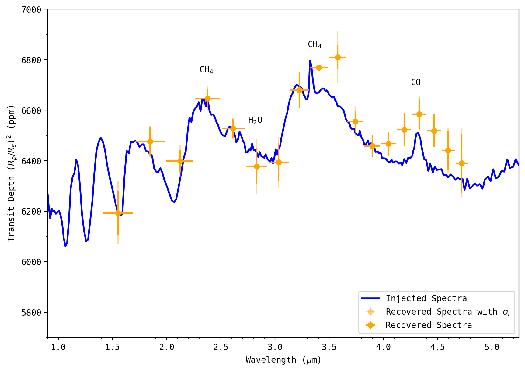
<Figure size 2000x1400 with 0 Axes>
By and large, the injected transit depths are well recovered across the spectra, with features such as H\(_2\)O and CH\(_4\) easily detected. There is a bit of an offset in data-points long-ward of 3.5 \(\mu\)m that could perhaps be due to changes in CO\(_2\) or H\(_2\)O absorption features from ice built up on the cryogenic window during the CV3 test. These wavelengths show some increases in time correlated noise (\(\sigma_r\)), which has been measured here, and the errors in the plot also show the transit depths with this error included.
The precisions from the ground-based test are very encouraging, with the best measured bin (which occurs in a clean part of the spectrum with high count rates) achieving near-photon limited transit depths measured to about 30 ppm in only 2 hours of data, and with minimal time correlated noise (\(\sigma_r\)).
For more robust error estimates, in practice the least-squares minimization performed here would be replaced by an MCMC routine. In addition, with actual transit data, the transit fit parameters (e.g. \(i\), \(a/R_{star}\), T\(_0\)) would also have to be first fit as well, as they can/will differ from literature estimates in high precision transit light curves as JWST will provide.