Advanced: NIRISS Imaging Tutorial Notebook

Advanced: NIRISS Imaging Tutorial Notebook#

Table of Contents#

Introduction
Examining uncalibrated data products
Stage 1 Processing
Stage 2 Processing
Stage 3 Processing
Visualize Detected Sources

Date published: January 24, 2024

1. Introduction #

In this notebook, we will process a NIRISS imaging dataset through the JWST calibration pipeline. The example dataset is from Program ID 1475 (PI: Boyer, CoI: Volk) which is a sky flat calibration program. NIRCam is used as the primary instrument with NIRISS as a coordinated parallel instrument. The NIRISS imaging dataset uses a 17-step dither pattern.

For illustrative purposes, we focus on data taken through the NIRISS F150W filter and start with uncalibrated data products. The files are named jw01475006001_02201_000nn_nis_uncal.fits, where nn refers to the dither step number which ranges from 01 - 17. See the “File Naming Schemes” documentation to learn more about the file naming convention.

In this notebook, we assume all uncalibrated fits files are saved in a directory named 1475_f150w.

Install pipeline and dependencies#

To make sure that the pipeline version is compatabile with the steps discussed below and the required dependencies and packages are installed, you can create a fresh conda environment and install the provided requirements.txt file:

conda create -n niriss_imaging_pipeline python=3.11
conda activate niriss_imaging_pipeline
pip install -r requirements.txt

Imports#

import os
import glob
import zipfile
import numpy as np
import urllib.request
from IPython.display import Image

# For visualizing images
import jdaviz
from jdaviz import Imviz

# Astropy routines for visualizing detected sources:
from astropy.table import Table
from astropy.coordinates import SkyCoord

# Configure CRDS
os.environ["CRDS_PATH"] = 'crds_cache'
os.environ["CRDS_SERVER_URL"] = "https://jwst-crds.stsci.edu"

# for JWST calibration pipeline
import jwst
from jwst import datamodels
from jwst.pipeline import Detector1Pipeline, Image2Pipeline, Image3Pipeline
from jwst.associations import asn_from_list
from jwst.associations.lib.rules_level3_base import DMS_Level3_Base

# To confirm which version of the pipeline you're running:
print(f"jwst pipeline version: {jwst.__version__}")
print(f"jdaviz version: {jdaviz.__version__}")

Download uncalibrated data products#

# APT program ID number:
pid = '01475'

# Set up directory to download uncalibrated data files:
data_dir = '1475_f150w/'
# Create directory if it does not exist
if not os.path.isdir(data_dir):
    os.mkdir(data_dir)

# Download uncalibrated data from Box into current directory:
boxlink = 'https://data.science.stsci.edu/redirect/JWST/jwst-data_analysis_tools/niriss_imaging/1475_f150w.zip'
boxfile = os.path.join(data_dir, '1475_f150w.zip')
urllib.request.urlretrieve(boxlink, boxfile)

zf = zipfile.ZipFile(boxfile, 'r')
zf.extractall()

2. Examining uncalibrated data products #

uncal_files = sorted(glob.glob(os.path.join(data_dir, '*_uncal.fits')))

Look at the first file to determine exposure parameters and practice using JWST datamodels#

# print file name
print(uncal_files[0])

# Open file as JWST datamodel
examine = datamodels.open(uncal_files[0])

# Print out exposure info
print("Instrument: " + examine.meta.instrument.name)
print("Filter: " + examine.meta.instrument.filter)
print("Pupil: " + examine.meta.instrument.pupil)
print("Number of integrations: {}".format(examine.meta.exposure.nints))
print("Number of groups: {}".format(examine.meta.exposure.ngroups))
print("Readout pattern: " + examine.meta.exposure.readpatt)
print("Dither position number: {}".format(examine.meta.dither.position_number))
print("\n")

From the above, we confirm that the data file is for the NIRISS instrument using the F150W filter in the Pupil Wheel crossed with the CLEAR filter in the Filter Wheel. This observation uses the NIS readout pattern, 16 groups per integration, and 1 integration per exposure. This data file is the 1st dither position in this exposure sequence. For more information about how JWST exposures are defined by up-the-ramp sampling, see the Understanding Exposure Times JDox article.

This metadata will be the same for all exposures in this observation other than the dither position number.

Display uncalibrated image#

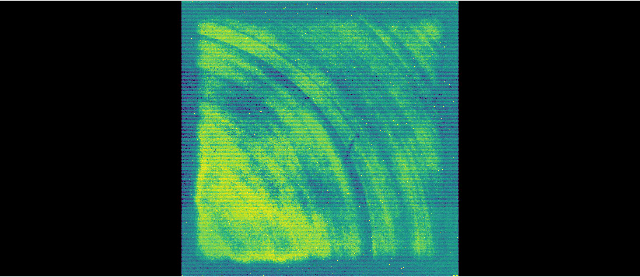
We can visualize an uncalibrated dataset that will show detector artifacts that will be removed when calibrating the data through the DETECTOR1 stage of the pipeline. Uncalibrated data files thus are 4D: nintegrations x ngroups x nrows x ncols. Here, we are visualizing the full detector (i.e., all columns and rows) and the 1st group.

We are using the Imviz tool within the jdaviz package to visualize the NIRISS image.

# Create an Imviz instance and set up default viewer
imviz_uncal = Imviz()
viewer_uncal = imviz_uncal.default_viewer

# Read in the science array for our visualization dataset:
uncal_science = examine.data

# Load the dataset into Imviz
imviz_uncal.load_data(uncal_science[0, 0, :, :])

# Visualize the dataset:
imviz_uncal.show()

Adjust settings for the viewer:

plotopt = imviz_uncal.plugins['Plot Options']
plotopt.stretch_function = 'sqrt'
plotopt.image_colormap = 'Viridis'
plotopt.stretch_preset = '99.5%'
plotopt.zoom_radius = 1024

The viewer looks like this:

viewer_uncal.save('./uncal_science.png')

Image('./uncal_science.png')

3. Stage 1 Processing #

Run the datasets through the Detector1 stage of the pipeline to apply detector level calibrations and create a countrate data product where slopes are fitted to the integration ramps. These *_rate.fits products are 2D (nrows x ncols), averaged over all integrations. 3D countrate data products (*_rateints.fits) are also created (nintegrations x nrows x ncols) which have the fitted ramp slopes for each integration.

The pipeline documentation discusses how to run the pipeline in the Python Interface, including how to configure pipeline steps and override reference files. By returning the results of the pipeline to a variable, the pipeline returns a datamodel. Note that the pipeline.call() method is preferred over the pipeline.run() method.

By default, all steps in the Detector1 stage of the pipeline are run for NIRISS except: the ipc correction step and the gain_scale step. Note that while the persistence step is set to run by default, this step does not automatically correct the science data for persistence. The persistence step creates a *_trapsfilled.fits file which is a model that records the number of traps filled at each pixel at the end of an exposure. This file would be used as an input to the persistence step, via the input_trapsfilled argument, to correct a science exposure for persistence. Since persistence is not well calibrated for NIRISS, we do not perform a persistence correction and thus turn off this step to speed up calibration and to not create files that will not be used in the subsequent analysis. This step can be turned off when running the pipeline in Python by doing:

rate_result = Detector1Pipeline.call(uncal,
                                     steps={'persistence': {'skip': True}})

The charge_migration step is particularly important for NIRISS images to mitigate apparent flux loss in resampled images due to the spilling of charge from a central pixel into its neighboring pixels (see Goudfrooij et al. 2023 for details). Charge migration occurs when the accumulated charge in a central pixel exceeds a certain signal limit, which is ~25,000 ADU. This step is turned on by default for NIRISS imaging, Wide Field Slitless Spectroscopy (WFSS), and Aperture Masking Interferometry (AMI) modes when using CRDS contexts of jwst_1159.pmap or later. Different signal limits for each filter are provided by the pars-chargemigrationstep parameter files. Users can specify a different signal limit by running this step with the signal_threshold flag and entering another signal limit in units of ADU.

As of CRDS context jwst_1155.pmap and later, the jump step of the DETECTOR1 stage of the pipeline will remove residuals associated with snowballs for NIRISS imaging, WFSS, and AMI modes. The default parameters for this correction, where expand_large_events set to True turns on the snowball halo removal algorithm, are specified in the pars-jumpstep parameter reference files. Users may wish to alter parameters to optimize removal of snowball residuals. Available parameters are discussed in the Detection and Flagging of Showers and Snowballs in JWST Technical Report (Regan 2023).

# Define directory to save output from detector1
det1_dir = 'detector1/'
# Create directory if it does not exist
if not os.path.isdir(det1_dir):
    os.mkdir(det1_dir)

# Run Detector1 stage of pipeline, specifying:
# output directory to save *_rate.fits files
# save_results flag set to True so the rate files are saved
# skipping the persistence step
    
for uncal in uncal_files:
    rate_result = Detector1Pipeline.call(uncal,
                                         output_dir=det1_dir,
                                         save_results=True,
                                         steps={'persistence': {'skip': True}})

Identify `*_rate.fits` files#

rate_files = sorted(glob.glob(os.path.join(det1_dir, '*_rate.fits')))

Verify which pipeline steps were run and which calibration reference files were applied#

The header contains information about which calibration steps were completed and skipped and which reference files were used to process the data.

# Read in file as datamodel
rate_f = datamodels.open(rate_files[0])

rate_f.meta.cal_step.instance

Check which reference files were used to calibrate the dataset:

rate_f.meta.ref_file.instance

Display rate image#

Visualize a countrate image, using the dataset from the first dither position as an example.

# Create an Imviz instance and set up default viewer
imviz_rate = Imviz()
viewer_rate = imviz_rate.default_viewer

# Read in the science array for our visualization dataset:
rate_science = rate_f.data

# Load the dataset into Imviz
imviz_rate.load_data(rate_science)

# Visualize the dataset:
imviz_rate.show()

plotopt = imviz_rate.plugins['Plot Options']
plotopt.stretch_function = 'sqrt'
plotopt.image_colormap = 'Viridis'
plotopt.stretch_preset = '95%'
plotopt.zoom_radius = 1024

The viewer looks like this:

viewer_rate.save('./rate_science.png')

Image('./rate_science.png')

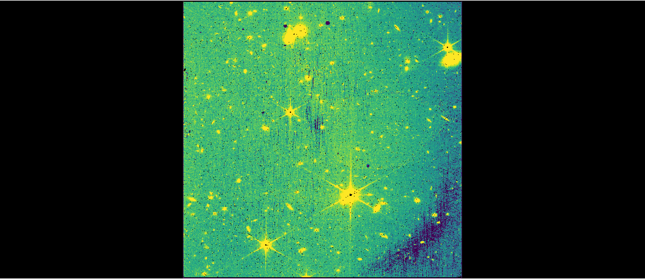
3. Stage 2 Processing #

In the Image2 stage of the pipeline, calibrated unrectified data products are created (*_cal.fits or *_calints.fits files, depending on whether the input files are *_rate.fits or *_rateints.fits).

In this pipeline processing stage, the world coordinate system (WCS) is assigned, the data are flat fielded, and a photometric calibration is applied to convert from units of countrate (ADU/s) to surface brightness (MJy/sr).

By default, the background subtraction step and the resampling step are turned off for NIRISS at this stage of the pipeline. The background subtraction is turned off since there is no background template for the imaging mode and the local background is removed during the background correction for photometric measurements around individual sources. The resampling step occurs during the Image3 stage by default. While the resampling step can be turned on during the Image2 stage to, e.g., generate a source catalog for each image, the data quality from the Image3 stage will be better since the bad pixels, which adversely affect both the centroids and photometry in individual images, will be mostly removed.

# Define directory to save output from Image2
image2_dir = 'image2/'
# Create directory if it does not exist
if not os.path.isdir(image2_dir):
    os.mkdir(image2_dir)

# Run Image2 stage of pipeline, specifying:
# output directory to save *_cal.fits files
# save_results flag set to True so the rate files are saved

for rate in rate_files:
    cal_result = Image2Pipeline.call(rate,
                                     output_dir=image2_dir,
                                     save_results=True)

Identify `*_cal.fits` files#

cal_files = sorted(glob.glob(os.path.join(image2_dir, '*_cal.fits')))

Verify which pipeline steps were run#

cal_f = datamodels.open(cal_files[0])

cal_f.meta.cal_step.instance

Check which reference files were used to calibrate the dataset:

cal_f.meta.ref_file.instance

Display cal image#

Visualize a calibrated image, using the dataset from the first dither position as an example.

# Create an Imviz instance and set up default viewer
imviz_cal = Imviz()
viewer_cal = imviz_cal.default_viewer

# Read in the science array for our visualization dataset:
cal_science = cal_f.data

# Load the dataset into Imviz
imviz_cal.load_data(cal_science)

# Visualize the dataset:
imviz_cal.show()

plotopt = imviz_cal.plugins['Plot Options']
plotopt.stretch_function = 'sqrt'
plotopt.image_colormap = 'Viridis'
plotopt.stretch_preset = '95%'
plotopt.zoom_radius = 1024

The viewer looks like this:

viewer_cal.save('./cal_science.png')

Image('./cal_science.png')

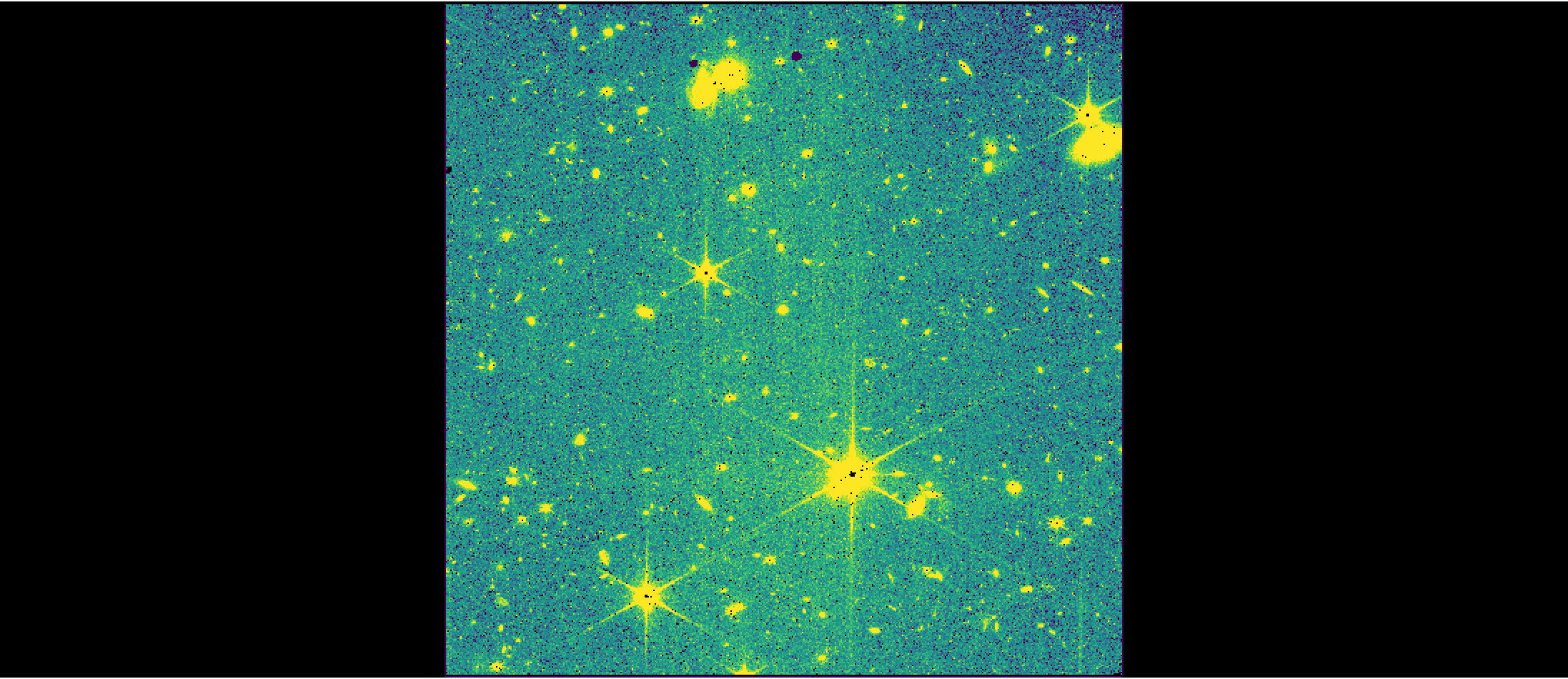
3. Stage 3 Processing #

In the Image3 stage of the pipeline, the individual *_cal.fits files for each of the dither positions are combined to one single distortion corrected image. First, an Association needs to be created to inform the pipeline that these individual exposures are linked together.

By default, the Image3 stage of the pipeline performs the following steps on NIRISS data:

tweakreg - creates source catalogs of pointlike sources for each input image. The source catalog for each input image is compared to each other to derive coordinate transforms to align the images relative to each other.
- As of CRDS context jwst_1156.pmap and later, the pars-tweakreg parameter reference file for NIRISS performs an absolute astrometric correction to GAIA data release 3 by default (i.e., the abs_refcat parameter is set to GAIADR3). Though this default correction generally improves results compared with not doing this alignment, it can sometimes result in poor performance in crowded or sparse fields, so users are encouraged to check astrometric accuracy and revisit this step if necessary.
- As of pipeline version 1.12.5, the default source finding algorithm is DAOStarFinder which can result in up to 0.5 pix uncertainties in the centroids for undersampled PSFs, like the NIRISS PSFs at short wavelengths (Goudfrooij 2022). There are plans to update the default algorithm to IRAFStarFinder in future pipeline versions.
skymatch - measures the background level from the sky to use as input into the subsequent outlier detection and resample steps.
outlier detection - flags any remaining cosmic rays, bad pixels, or other artifacts not already flagged during the DETECTOR1 stage of the pipeline, using all input images to create a median image so that outliers in individual images can be identified.
resample - resamples each input image based on its WCS and distortion information and creates a single undistorted image.
source catalog - creates a catalog of detected sources along with measured photometries and morphologies (i.e., point-like vs extended). Useful for quicklooks, but optimization is likely needed for specific science cases, which is an on-going investigation for the NIRISS team. Users may wish to experiment with changing the snr_threshold and deblend options. Modifications to the following parameters will not significantly improve data quality and it is advised to keep them at their default values: aperture_ee1, aperture_ee2, aperture_ee3, ci1_star_threshold, ci2_star_threshold.

Create Association File#

An association file lists the exposures to calibrated together in Stage 3 of the pipeline. Note that an association file is available for download from MAST, with a filename of *_asn.json. Here we show how to create an association file to point to the data products created when processing data through the pipeline. Note that the output products will have a rootname that is specified by the product_name in the association file. For this tutorial, the rootname of the output products will be image3_association.

# Create a Level 3 Association
associations = asn_from_list.asn_from_list(cal_files, 
                                           rule=DMS_Level3_Base, 
                                           product_name='image3_association')

associations.data['asn_type'] = 'image3'
associations.data['program'] = pid

# Format association as .json file
asn_filename, serialized = associations.dump(format="json")

# Write out association file
with open(asn_filename, "w") as fd:
    fd.write(serialized)

Run Image3 stage of the pipeline#

Given the grouped exposures in the association file, the Image3 stage of the pipeline will produce:

a *_cr.fits file produced by the outlier_detection step, where the DQ array marks the pixels flagged as outliers.
a final combined, rectified image with name *_i2d.fits,
a source catalog with name *_cat.ecsv,
a segmentation map file (*_segm.fits) which has integer values at the pixel locations where a source is detected where the pixel values match the source ID number in the catalog.

# Define directory to save output from Image2
image3_dir = 'image3/'
# Create directory if it does not exist
if not os.path.isdir(image3_dir):
    os.mkdir(image3_dir)

# Run Stage 3
i2d_result = Image3Pipeline.call(asn_filename, 
                                 output_dir=image3_dir,
                                 save_results=True)

Verify which pipeline steps were run#

# Identify *_i2d file and open as datamodel
i2d = glob.glob(os.path.join(image3_dir, "*_i2d.fits"))[0]
i2d_f = datamodels.open(i2d)

i2d_f.meta.cal_step.instance

Check which reference files were used to calibrate the dataset:

i2d_f.meta.ref_file.instance

Display combined image#

Visualize the drizzle-combined image.

# Create an Imviz instance and set up default viewer
imviz_i2d = Imviz()
viewer_i2d = imviz_i2d.default_viewer

# Read in the science array for our visualization dataset:
i2d_science = i2d_f.data

# Load the dataset into Imviz
imviz_i2d.load_data(i2d_science)

# Visualize the dataset:
imviz_i2d.show()

plotopt = imviz_i2d.plugins['Plot Options']
plotopt.stretch_function = 'sqrt'
plotopt.image_colormap = 'Viridis'
plotopt.stretch_preset = '95%'
plotopt.zoom_radius = 1024

The viewer looks like this:

viewer_i2d.save('./i2d_science.png')

Image('./i2d_science.png')

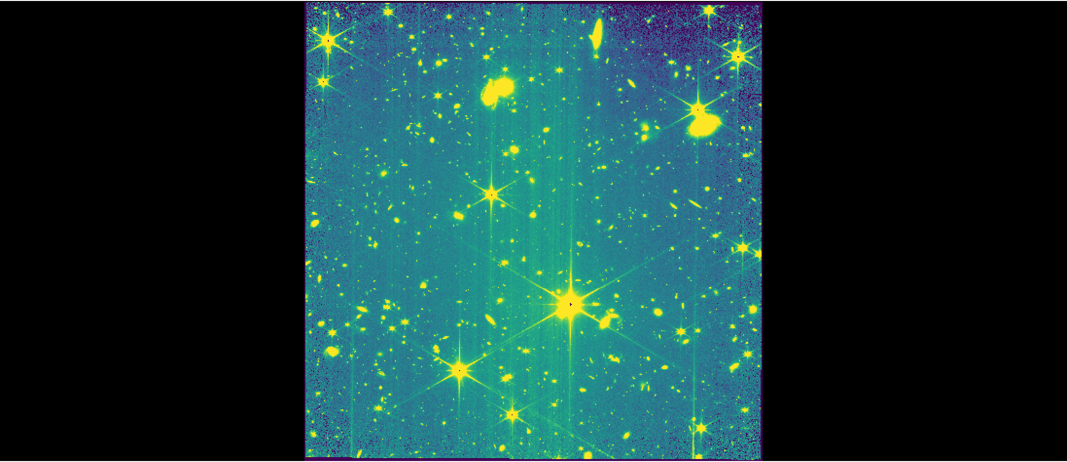
Visualize Detected Sources #

Using the source catalog created by the IMAGE3 stage of the pipeline, mark the detected sources, using different markers for point sources and extended sources. The source catalog is saved in image3/image3_association_cat.ecsv file. We will need to read in the i2d file again to make sure the world coordinate system (WCS) info is read in.

Read in catalog file and identify point/extended sources#

catalog_file = glob.glob(os.path.join(image3_dir, "*_cat.ecsv"))[0]
catalog = Table.read(catalog_file)

# To identify point/extended sources, use the 'is_extended' column in the source catalog
pt_src, = np.where(~catalog['is_extended'])
ext_src, = np.where(catalog['is_extended'])

# Define coordinates of point and extended sources
pt_coord = Table({'coord': [SkyCoord(ra=catalog['sky_centroid'][pt_src].ra,
                                     dec=catalog['sky_centroid'][pt_src].dec)]})
ext_coord = Table({'coord': [SkyCoord(ra=catalog['sky_centroid'][ext_src].ra,
                                      dec=catalog['sky_centroid'][ext_src].dec)]})

Mark the extended and point sources on the image#

Display combined image:

# Read in i2d file to Imviz
imviz_cat = Imviz()
viewer_cat = imviz_cat.default_viewer
imviz_cat.load_data(i2d)
imviz_cat.show()

# Adjust settings for viewer
plotopt = imviz_cat.plugins['Plot Options']
plotopt.stretch_function = 'sqrt'
plotopt.image_colormap = 'Viridis'
plotopt.stretch_preset = '95%'
plotopt.zoom_radius = 1024

Point sources will be marked by small pink circles and extended sources will be marked by larger white circles.

# Add marker for point sources:
viewer_cat.marker = {'color': 'pink', 'markersize': 50, 'fill': False}

viewer_cat.add_markers(pt_coord, use_skycoord=True, marker_name='point_sources')

# Add marker for extended sources:
viewer_cat.marker = {'color': 'white', 'markersize': 100, 'fill': False}

viewer_cat.add_markers(ext_coord, use_skycoord=True, marker_name='extended_sources')

Viewer looks like this:

viewer_cat.save('./i2d_markers.png')

Image('./i2d_markers.png')

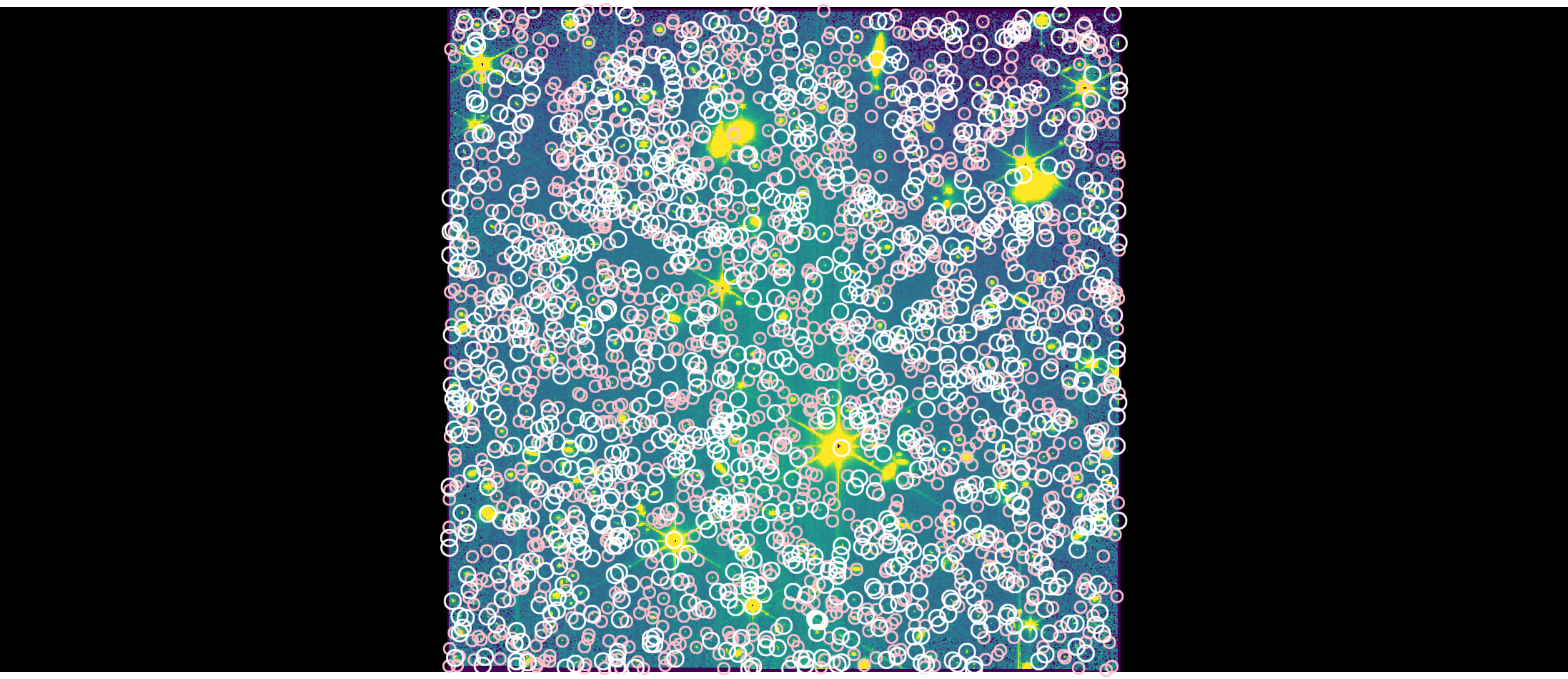
From zoooming in on different portions of the image, we can see that some saturated point sources are erroneously labeled as point sources, some extended and saturated objects are not detected, parts of diffraction spikes are sometimes detected as “extended sources”, and in some cases, the detected source centroid is offset from the center of a source. It is recommended for users to optimize source detection for their science goals using either their own tools or by updating parameters to the source_catalog step of the pipeline.

Advanced: NIRISS Imaging Tutorial Notebook

Contents

Advanced: NIRISS Imaging Tutorial Notebook#

Table of Contents#

1. Introduction#

Install pipeline and dependencies#

Imports#

Download uncalibrated data products#

2. Examining uncalibrated data products#

Look at the first file to determine exposure parameters and practice using JWST datamodels#

Display uncalibrated image#

3. Stage 1 Processing #

Identify *_rate.fits files#

Verify which pipeline steps were run and which calibration reference files were applied#

Display rate image#

3. Stage 2 Processing #

Identify *_cal.fits files#

Verify which pipeline steps were run#

Display cal image#

3. Stage 3 Processing #

Create Association File#

Run Image3 stage of the pipeline#

Verify which pipeline steps were run#

Display combined image#

Visualize Detected Sources#

Read in catalog file and identify point/extended sources#

Mark the extended and point sources on the image#

1. Introduction #

2. Examining uncalibrated data products #

Identify `*_rate.fits` files#

Identify `*_cal.fits` files#

Visualize Detected Sources #