Extended Aperture Photometry

Use case: Measure galaxy photometry in a field. Related to JDox Science Use Case #22.
Data: WST simulated NIRCam images from JADES JWST GTO extragalactic blank field.
(Williams et al. 2018) https://ui.adsabs.harvard.edu/abs/2018ApJS..236…33W.
Tools: photutils, matplotlib, scipy, scikit.
Cross-intrument: potentially MIRI.
Documentation: This notebook is part of a STScI’s larger post-pipeline Data Analysis Tools Ecosystem.

Introduction

This notebook uses photutils to detect objects/galaxies in NIRCam deep imaging. Detections are first made in a F200W image, then isophotal photometry is obtained in all 9 filters (F090W, F115W, F150W, F200W, F277W, F335M, F356W, F410M, F444W). The catalog is loaded back in and some simple analysis is performed on the full catalog and on an individual galaxy.

The notebook analyzes only the central 1000 x 1000 pixels (30” x 30”) of the full JADES simulation. These cutouts have been staged at STScI with permission from the authors (Williams et al.).

NOTE: The photometry is aperture matched, but no PSF corrections are made. For more accurate color measurements, PSF corrections should be implemented, given the large range of wavelengths (and thus PSF FWHM) spanning a factor of >4.

NOTE: The simulated JADES images have different units (e-/s) than JWST pipeline products (MJy/sr).

NOTE: An exposure map is missing but required to calculate flux uncertainties.

To Do

• PSF corrections

• Check accuracy of photometry against simulated JADES catalog

• Exposure map required for input to error calculation

• ABmag units cannot be written to ecsv file (astropy update coming soon)

• plot with text labels looks horrible (I wish cursor hover would show id number instead)

• Fix plot secondary axis: mag vs. flux

• requirements.txt file – but I don’t know what versions are “required”

• rest of Robel’s comments: https://github.com/spacetelescope/dat_pyinthesky/pull/82#pullrequestreview-355206337

Download WEBBPSF Data

import os
import tarfile
import urllib.request

boxlink = 'https://stsci.box.com/shared/static/34o0keicz2iujyilg4uz617va46ks6u9.gz'                                                           
boxfile = './webbpsf-data/webbpsf-data-1.0.0.tar.gz'

webbpsf_folder = './webbpsf-data'

# Check whether the specified path exists or not
isExist = os.path.exists(webbpsf_folder)
if not isExist:
  # Create a new directory because it does not exist 
  os.makedirs(webbpsf_folder)
    
urllib.request.urlretrieve(boxlink, boxfile)
gzf = tarfile.open(boxfile)
gzf.extractall(webbpsf_folder)

Import packages

import os

import numpy as np

from astropy.convolution import convolve
from astropy.io import fits
from astropy.stats import gaussian_fwhm_to_sigma
from astropy.table import QTable
import astropy.units as u
from astropy.visualization import make_lupton_rgb, SqrtStretch, ImageNormalize, simple_norm
import astropy.wcs as wcs

from photutils.background import Background2D, MedianBackground
from photutils.segmentation import (detect_sources, deblend_sources, SourceCatalog,
                                    make_2dgaussian_kernel, SegmentationImage)
from photutils.utils import calc_total_error

Matplotlib setup for plotting

There are two versions

• notebook – gives interactive plots, but makes the overall notebook a bit harder to scroll

• inline – gives non-interactive plots for better overall scrolling

import matplotlib.pyplot as plt
import matplotlib as mpl

# Use this version for non-interactive plots (easier scrolling of the notebook)
%matplotlib inline

# Use this version if you want interactive plots
# %matplotlib notebook

# These gymnastics are needed to make the sizes of the figures
# be the same in both the inline and notebook versions
%config InlineBackend.print_figure_kwargs = {'bbox_inches': None}

mpl.rcParams['savefig.dpi'] = 80
mpl.rcParams['figure.dpi'] = 80

Create list of images to be loaded and analyzed

baseurl = 'https://data.science.stsci.edu/redirect/JWST/jwst-data_analysis_tools/nircam_photometry/'

filters = 'F090W F115W F150W F200W F277W F335M F356W F410M F444W'.split()

# Data images [e-/s]
imagefiles = {}
for filt in filters:
    filename = f'jades_jwst_nircam_goods_s_crop_{filt}.fits'
    imagefiles[filt] = os.path.join(baseurl, filename)

# Weight images (Inverse Variance Maps; IVM)
weightfiles = {}
for filt in filters:
    filename = f'jades_jwst_nircam_goods_s_crop_{filt}_wht.fits'
    weightfiles[filt] = os.path.join(baseurl, filename)

Load detection image: F200W

filt = 'F200W'
infile = imagefiles[filt]
hdu = fits.open(infile)
data = hdu[0].data
imwcs = wcs.WCS(hdu[0].header, hdu)

weight = fits.open(weightfiles[filt])[0].data

Report image size and field of view

ny, nx = data.shape
pixscale = wcs.utils.proj_plane_pixel_scales(imwcs)[0] 
pixscale *= imwcs.wcs.cunit[0].to('arcsec')
outline = '%d x %d pixels' % (ny, nx)
outline += ' = %g" x %g"' % (ny * pixscale, nx * pixscale)
outline += ' (%.2f" / pixel)' % pixscale
print(outline)

1000 x 1000 pixels = 30" x 30" (0.03" / pixel)

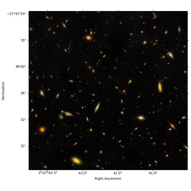
Create color image (optional)

# 3 NIRCam short wavelength channel images
r = fits.open(imagefiles['F200W'])[0].data
g = fits.open(imagefiles['F150W'])[0].data
b = fits.open(imagefiles['F090W'])[0].data

rgb = make_lupton_rgb(r, g, b, Q=5, stretch=0.02)  # , minimum=-0.001

fig = plt.figure(figsize=(8, 8))
ax = plt.subplot(projection=imwcs)
plt.imshow(rgb, origin='lower')
plt.xlabel('Right Ascension')
plt.ylabel('Declination')
fig.tight_layout()
plt.subplots_adjust(left=0.15)

Detect Sources and Deblend using photutils

https://photutils.readthedocs.io/en/latest/segmentation.html

# For detection, requiring 5 connected pixels 2-sigma above background

# Measure background and set detection threshold
bkg_estimator = MedianBackground()
bkg = Background2D(data, (50, 50), filter_size=(3, 3), bkg_estimator=bkg_estimator)
threshold = bkg.background + (2. * bkg.background_rms)

# Before detection, smooth image with Gaussian FWHM = 3 pixels
smooth_kernel = make_2dgaussian_kernel(3.0, size=3)
convolved_data = convolve(data, smooth_kernel)

# Detect and deblend
segm_detect = detect_sources(convolved_data, threshold, npixels=5)

segm_deblend = deblend_sources(convolved_data, segm_detect, npixels=5, nlevels=32, contrast=0.001)

# Save segmentation map of detected objects
segm_hdu = fits.PrimaryHDU(segm_deblend.data.astype(np.uint32), header=imwcs.to_header())
segm_hdu.writeto('JADES_detections_segm.fits', overwrite=True)

Measure photometry (and more) in detection image

https://photutils.readthedocs.io/en/latest/segmentation.html#centroids-photometry-and-morphological-properties

#error = bkg.background_rms
# Input weight should be exposure map. Fudging for now.
error = calc_total_error(data, bkg.background_rms, weight/500)
#cat = source_properties(data-bkg.background, segm_deblend, wcs=imwcs, background=bkg.background, error=error)
cat = SourceCatalog(data-bkg.background, segm_deblend, wcs=imwcs, background=bkg.background, error=error)

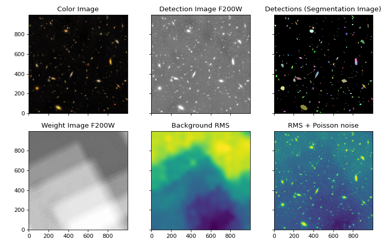
Show detections alongside images (optional)

fig, ax = plt.subplots(2, 3, sharex=True, sharey=True, figsize=(9.5, 6))
# For RA,Dec axes instead of pixels, add: , subplot_kw={'projection': imwcs})

# Color image
ax[0, 0].imshow(rgb, origin='lower')
ax[0, 0].set_title('Color Image')

# Data
norm = simple_norm(data, 'sqrt', percent=99.)
ax[0, 1].imshow(data, origin='lower', cmap='Greys_r', norm=norm)
ax[0, 1].set_title('Detection Image F200W')

# Segmentation map
cmap = segm_deblend.make_cmap(seed=12345)
ax[0, 2].imshow(segm_deblend, origin='lower', cmap=cmap, interpolation='nearest')
ax[0, 2].set_title('Detections (Segmentation Image)')

# Weight
ax[1, 0].imshow(weight, origin='lower', cmap='Greys_r', vmin=0)
ax[1, 0].set_title('Weight Image F200W')

# RMS
ax[1, 1].imshow(bkg.background_rms, origin='lower', norm=None)
ax[1, 1].set_title('Background RMS')

# Total error including Poisson noise
norm = simple_norm(error, 'sqrt', percent=99.)
ax[1, 2].imshow(error, origin='lower', norm=norm)
ax[1, 2].set_title('RMS + Poisson noise')

fig.tight_layout()

View all measured quantities in detection image (optional)

cat.to_table()

QTable length=326

label	xcentroid	ycentroid	sky_centroid	bbox_xmin	bbox_xmax	bbox_ymin	bbox_ymax	area	semimajor_sigma	semiminor_sigma	orientation	eccentricity	min_value	max_value	local_background	segment_flux	segment_fluxerr	kron_flux	kron_fluxerr
			deg,deg					pix2	pix	pix	deg
int32	float64	float64	SkyCoord	int64	int64	int64	int64	float64	float64	float64	float64	float64	float64	float64	float64	float64	float64	float64	float64
1	466.24461350033647	8.7975642602371	53.17381009103326,-27.805320830365776	460	472	3	14	101.0	3.121883592723396	1.687718238373556	-44.478947493786606	0.8412740063312978	0.0006697164628791134	0.03003565456943476	0.0	0.8863594626861904	0.04333105379347733	1.1523646398846878	0.05542864325311204
2	104.80681791619067	18.082129411035602	53.17721522973072,-27.805243193448323	95	116	10	27	271.0	4.4330760205526705	2.8904310038200527	-26.54972210581966	0.7582062720085906	0.001169592682614256	0.05683289995260978	0.0	3.3850931796608226	0.10096273567434758	4.064307886560463	0.1178471432803697
3	15.04416396551755	13.21870964358083	53.178060898531776,-27.805283643045666	14	16	12	14	8.0	0.8501945455843772	0.6682678017840504	-38.1612276642421	0.6182042301587309	0.0035728101756059504	0.006067336431199741	0.0	0.04072228096572398	0.011222825585360583	0.10086850698470742	0.02315230578296353
4	710.3242889701858	14.259777138086877	53.17151058505514,-27.805275444028442	708	712	12	17	25.0	1.2749753643104456	1.117371994707132	-59.26178196559024	0.4816073152747641	0.0013530635966815864	0.015100956012602468	0.0	0.15496901383687856	0.018575211927226793	0.19011686546526946	0.023625589169720226
5	434.5294891713508	22.219091527997158	53.17410887322447,-27.8052089643638	424	447	14	30	268.0	3.9551276120227397	2.6287674709150584	-8.140060370882344	0.7471566761152122	-0.0003420958396561837	0.10656058422736421	0.0	3.6147863822998016	0.08773502088121837	4.278741209374845	0.10086436727140968
6	289.38802515014896	17.281765562153954	53.17547627056455,-27.805250009193262	287	291	15	20	17.0	1.2913044931147235	1.1978568863866517	68.12270923149859	0.37349256122504115	0.0019512862197305747	0.008797215945005498	0.0	0.08513804286457863	0.0166428570162664	0.34384198668200716	0.045989916939691816
7	640.4863091995317	17.773429154661983	53.17216853452775,-27.805246129692247	638	642	15	20	21.0	1.5124916692884618	0.8803106550282112	-64.72678377811528	0.8131696183154983	0.0003576250881105088	0.009946935910809692	0.0	0.09708323832036175	0.014462494201596655	0.17695836262605436	0.026075310664432968
8	762.762291737285	28.289914155884627	53.171016553902064,-27.805158549648304	754	771	21	36	200.0	3.160315774736445	2.3536095208280066	37.520056617399476	0.6673561574146197	-0.0001941792050655057	0.10556121967783572	0.0	3.8212752545169955	0.08847910158114891	3.9811392641181644	0.09150995786991047
9	801.0706722163886	32.58026118517374	53.17065564474934,-27.805122812753073	799	804	31	34	12.0	1.3349434908844906	0.6567170220834244	-28.75519616047975	0.8706270208190223	0.0018856854900614819	0.009336017794193286	0.0	0.05935203501404956	0.012189355644992149	0.17003504172320322	0.027778386430149567
...	...	...	...	...	...	...	...	...	...	...	...	...	...	...	...	...	...	...	...
318	13.440867157588091	884.6702424852333	53.17807510890577,-27.798021546451285	6	21	877	892	184.0	3.2736106643758327	3.140562210245422	-6.296591150380023	0.2821942888203486	0.0014361034419094758	0.03495382468946091	0.0	2.107846654516414	0.10758977389933193	3.4100106248507016	0.154602699729525
319	7.1117930282611415	891.8881745003442	53.17813472440638,-27.797961391261722	5	11	889	895	30.0	1.6388613720493859	1.3203695638683461	-73.17086230879917	0.5923744840346211	0.0019018454919824644	0.01347560203904176	0.0	0.22372547016303176	0.03584393685439291	0.6688447648831534	0.07533566959001846
320	143.92969676102126	953.6973600108524	53.17684577662435,-27.797446433611444	139	149	950	957	59.0	2.6507581110195266	1.3964068465385502	25.19703083525805	0.849992199281631	0.0021617009219625062	0.021165230633174926	0.0	0.5681924075559929	0.05743803199966468	1.254760987505672	0.10492362090925443
321	142.746173256619	959.5389917866399	53.176856920479636,-27.797397752374	139	147	957	963	48.0	2.1427436610213637	1.2555061677914512	-35.47427950196171	0.8103588434156908	0.00047583665796055224	0.030453184966657037	0.0	0.5637982114834339	0.0568718012708143	0.8893801784930943	0.08214060528713435
322	790.4887212488912	955.3594081523211	53.17075490894491,-27.797432983032667	784	797	951	959	96.0	2.688108198906902	1.894318151554492	8.747812174119948	0.7095023299745098	0.0005767950066928708	0.04023169644016939	0.0	1.1312940047504931	0.07957309918878556	1.6767674397202548	0.10950450078803163
323	797.3519286211066	965.5980743288513	53.17069024984349,-27.797347663631648	792	802	958	974	118.0	2.982037604259938	1.7682402286086438	79.7037323997118	0.8052291475056543	0.002333420221800177	0.08761686954182783	0.0	2.1012337463829494	0.1059056481884639	2.822766635652669	0.13081451901117752
324	790.7983558965504	979.5822296300561	53.17075198078638,-27.79723112632807	781	799	972	989	133.0	4.506451359665357	1.493045462994405	-44.19824469199431	0.9435209394229406	-0.001248849458808359	0.06943444193177313	0.0	2.002750597650743	0.10372107669936124	2.813577038594517	0.13630578304670982
325	307.63744942017837	990.2252882785789	53.17530354876154,-27.797142160721208	305	311	987	994	40.0	1.956531435792076	1.170389373708425	-59.658382281967256	0.8013497909948246	0.0017972712412996086	0.030535860130823354	0.0	0.4113390990802942	0.04757817769364764	0.7761334792977134	0.0762793986919714
326	306.8980749204495	997.3902653315687	53.17531050813543,-27.797082452050926	302	312	994	999	48.0	2.523806433484608	1.384440592182262	12.21698945753027	0.8361160446765955	0.002853197675265836	0.02047051119926145	0.0	0.5267357091594782	0.05337859775778076	0.729590727062627	0.06944105571892703

Only keep some quantities

columns = 'label xcentroid ycentroid sky_centroid area semimajor_sigma semiminor_sigma ellipticity orientation gini'.split()
tbl = cat.to_table(columns=columns)
tbl.rename_column('semimajor_sigma', 'a')
tbl.rename_column('semiminor_sigma', 'b')

tbl

QTable length=326

label	xcentroid	ycentroid	sky_centroid	area	a	b	ellipticity	orientation	gini
			deg,deg	pix2	pix	pix		deg
int32	float64	float64	SkyCoord	float64	float64	float64	float64	float64	float64
1	466.24461350033647	8.7975642602371	53.17381009103326,-27.805320830365776	101.0	3.121883592723396	1.687718238373556	0.4593910412587602	-44.478947493786606	0.3750841422808698
2	104.80681791619067	18.082129411035602	53.17721522973072,-27.805243193448323	271.0	4.4330760205526705	2.8904310038200527	0.34798523859744157	-26.54972210581966	0.4292034166747856
3	15.04416396551755	13.21870964358083	53.178060898531776,-27.805283643045666	8.0	0.8501945455843772	0.6682678017840504	0.21398248759086114	-38.1612276642421	0.10521135944081007
4	710.3242889701858	14.259777138086877	53.17151058505514,-27.805275444028442	25.0	1.2749753643104456	1.117371994707132	0.12361287442487268	-59.26178196559024	0.33737600483155716
5	434.5294891713508	22.219091527997158	53.17410887322447,-27.8052089643638	268.0	3.9551276120227397	2.6287674709150584	0.33535204706817323	-8.140060370882344	0.5363680123723463
6	289.38802515014896	17.281765562153954	53.17547627056455,-27.805250009193262	17.0	1.2913044931147235	1.1978568863866517	0.07236682535090477	68.12270923149859	0.18041073594089005
7	640.4863091995317	17.773429154661983	53.17216853452775,-27.805246129692247	21.0	1.5124916692884618	0.8803106550282112	0.41797322067741016	-64.72678377811528	0.257339933672325
8	762.762291737285	28.289914155884627	53.171016553902064,-27.805158549648304	200.0	3.160315774736445	2.3536095208280066	0.2552612812799423	37.520056617399476	0.5417393494467531
9	801.0706722163886	32.58026118517374	53.17065564474934,-27.805122812753073	12.0	1.3349434908844906	0.6567170220834244	0.5080563135685205	-28.75519616047975	0.28793220448127643
...	...	...	...	...	...	...	...	...	...
318	13.440867157588091	884.6702424852333	53.17807510890577,-27.798021546451285	184.0	3.2736106643758327	3.140562210245422	0.04064272382121481	-6.296591150380023	0.33246937212374045
319	7.1117930282611415	891.8881745003442	53.17813472440638,-27.797961391261722	30.0	1.6388613720493859	1.3203695638683461	0.1943372475627806	-73.17086230879917	0.2490826303025817
320	143.92969676102126	953.6973600108524	53.17684577662435,-27.797446433611444	59.0	2.6507581110195266	1.3964068465385502	0.47320472557133164	25.19703083525805	0.2823870637944277
321	142.746173256619	959.5389917866399	53.176856920479636,-27.797397752374	48.0	2.1427436610213637	1.2555061677914512	0.41406609169806174	-35.47427950196171	0.3421221334166607
322	790.4887212488912	955.3594081523211	53.17075490894491,-27.797432983032667	96.0	2.688108198906902	1.894318151554492	0.29529691091868937	8.747812174119948	0.3790106203018768
323	797.3519286211066	965.5980743288513	53.17069024984349,-27.797347663631648	118.0	2.982037604259938	1.7682402286086438	0.4070362405616029	79.7037323997118	0.4740381190737283
324	790.7983558965504	979.5822296300561	53.17075198078638,-27.79723112632807	133.0	4.506451359665357	1.493045462994405	0.6686871012615841	-44.19824469199431	0.42319913307021234
325	307.63744942017837	990.2252882785789	53.17530354876154,-27.797142160721208	40.0	1.956531435792076	1.170389373708425	0.40180395147364023	-59.658382281967256	0.35192342998474957
326	306.8980749204495	997.3902653315687	53.17531050813543,-27.797082452050926	48.0	2.523806433484608	1.384440592182262	0.4514473955632282	12.21698945753027	0.2410634775489439

Convert measured fluxes (data units) to magnitudes

https://docs.astropy.org/en/stable/units/

https://docs.astropy.org/en/stable/units/equivalencies.html#photometric-zero-point-equivalency

https://docs.astropy.org/en/stable/units/logarithmic_units.html#logarithmic-units

# not detected: mag =  99; magerr = 1-sigma upper limit assuming zero flux
# not observed: mag = -99; magerr = 0
def fluxes2mags(flux, fluxerr):
    nondet = flux < 0  # Non-detection if flux is negative
    unobs = (fluxerr <= 0) + (fluxerr == np.inf)  # Unobserved if flux uncertainty is negative or infinity

    mag = flux.to(u.ABmag)
    magupperlimit = fluxerr.to(u.ABmag)  # 1-sigma upper limit if flux=0

    mag = np.where(nondet, 99 * u.ABmag, mag)
    mag = np.where(unobs, -99 * u.ABmag, mag)

    magerr = 2.5 * np.log10(1 + fluxerr/flux) 
    magerr = magerr.value * u.ABmag

    magerr = np.where(nondet, magupperlimit, magerr)
    magerr = np.where(unobs, 0*u.ABmag, magerr)
    
    return mag, magerr

# Includes features I couldn't find in astropy:
# mag = 99 / -99 for non-detections / unobserved
# flux uncertainties -> mag uncertainties

Multiband photometry using isophotal apertures defined in detection image

(Similar to running SourceExtractor in double-image mode)

filters = 'F090W F115W F150W F200W F277W F335M F356W F410M F444W'.split()
for filt in filters:
    infile = imagefiles[filt]
    print(filt)
    print(infile)
    print(weightfiles[filt])
    hdu = fits.open(infile)
    data = hdu[0].data
    zp = hdu[0].header['ABMAG'] * u.ABmag  # zeropoint
    weight = fits.open(weightfiles[filt])[0].data
    
    # Measure background
    bkg = Background2D(data, (50, 50), filter_size=(3, 3), bkg_estimator=bkg_estimator)
    #error = bkg.background_rms
    error = calc_total_error(data, bkg.background_rms, weight/500)
                             
    # Measure properties in each image of previously detected objects 
    filtcat = SourceCatalog(data-bkg.background, segm_deblend, wcs=imwcs, background=bkg.background, error=error)

    # Convert measured fluxes to fluxes in nJy and to AB magnitudes
    filttbl = filtcat.to_table()
    tbl[filt+'_flux']    = flux    = filttbl['segment_flux']     * zp.to(u.nJy)
    tbl[filt+'_fluxerr'] = fluxerr = filttbl['segment_fluxerr'] * zp.to(u.nJy)

    mag, magerr = fluxes2mags(flux, fluxerr)
    #mag = mag * u.ABmag  # incompatible with file writing
    tbl[filt+'_mag']    = mag.value
    tbl[filt+'_magerr'] = magerr.value

F090W
https://data.science.stsci.edu/redirect/JWST/jwst-data_analysis_tools/nircam_photometry/jades_jwst_nircam_goods_s_crop_F090W.fits
https://data.science.stsci.edu/redirect/JWST/jwst-data_analysis_tools/nircam_photometry/jades_jwst_nircam_goods_s_crop_F090W_wht.fits

/opt/hostedtoolcache/Python/3.11.11/x64/lib/python3.11/site-packages/astropy/units/function/logarithmic.py:67: RuntimeWarning: invalid value encountered in log10
  return dex.to(self._function_unit, np.log10(x))

F115W
https://data.science.stsci.edu/redirect/JWST/jwst-data_analysis_tools/nircam_photometry/jades_jwst_nircam_goods_s_crop_F115W.fits
https://data.science.stsci.edu/redirect/JWST/jwst-data_analysis_tools/nircam_photometry/jades_jwst_nircam_goods_s_crop_F115W_wht.fits

/opt/hostedtoolcache/Python/3.11.11/x64/lib/python3.11/site-packages/astropy/units/function/logarithmic.py:67: RuntimeWarning: invalid value encountered in log10
  return dex.to(self._function_unit, np.log10(x))
/opt/hostedtoolcache/Python/3.11.11/x64/lib/python3.11/site-packages/astropy/units/quantity.py:658: RuntimeWarning: invalid value encountered in log10
  result = super().__array_ufunc__(function, method, *arrays, **kwargs)

F150W
https://data.science.stsci.edu/redirect/JWST/jwst-data_analysis_tools/nircam_photometry/jades_jwst_nircam_goods_s_crop_F150W.fits
https://data.science.stsci.edu/redirect/JWST/jwst-data_analysis_tools/nircam_photometry/jades_jwst_nircam_goods_s_crop_F150W_wht.fits

F200W
https://data.science.stsci.edu/redirect/JWST/jwst-data_analysis_tools/nircam_photometry/jades_jwst_nircam_goods_s_crop_F200W.fits
https://data.science.stsci.edu/redirect/JWST/jwst-data_analysis_tools/nircam_photometry/jades_jwst_nircam_goods_s_crop_F200W_wht.fits

F277W
https://data.science.stsci.edu/redirect/JWST/jwst-data_analysis_tools/nircam_photometry/jades_jwst_nircam_goods_s_crop_F277W.fits
https://data.science.stsci.edu/redirect/JWST/jwst-data_analysis_tools/nircam_photometry/jades_jwst_nircam_goods_s_crop_F277W_wht.fits

F335M
https://data.science.stsci.edu/redirect/JWST/jwst-data_analysis_tools/nircam_photometry/jades_jwst_nircam_goods_s_crop_F335M.fits
https://data.science.stsci.edu/redirect/JWST/jwst-data_analysis_tools/nircam_photometry/jades_jwst_nircam_goods_s_crop_F335M_wht.fits

F356W
https://data.science.stsci.edu/redirect/JWST/jwst-data_analysis_tools/nircam_photometry/jades_jwst_nircam_goods_s_crop_F356W.fits
https://data.science.stsci.edu/redirect/JWST/jwst-data_analysis_tools/nircam_photometry/jades_jwst_nircam_goods_s_crop_F356W_wht.fits

F410M
https://data.science.stsci.edu/redirect/JWST/jwst-data_analysis_tools/nircam_photometry/jades_jwst_nircam_goods_s_crop_F410M.fits
https://data.science.stsci.edu/redirect/JWST/jwst-data_analysis_tools/nircam_photometry/jades_jwst_nircam_goods_s_crop_F410M_wht.fits

/opt/hostedtoolcache/Python/3.11.11/x64/lib/python3.11/site-packages/astropy/units/function/logarithmic.py:67: RuntimeWarning: invalid value encountered in log10
  return dex.to(self._function_unit, np.log10(x))
/opt/hostedtoolcache/Python/3.11.11/x64/lib/python3.11/site-packages/astropy/units/quantity.py:658: RuntimeWarning: invalid value encountered in log10
  result = super().__array_ufunc__(function, method, *arrays, **kwargs)

F444W
https://data.science.stsci.edu/redirect/JWST/jwst-data_analysis_tools/nircam_photometry/jades_jwst_nircam_goods_s_crop_F444W.fits
https://data.science.stsci.edu/redirect/JWST/jwst-data_analysis_tools/nircam_photometry/jades_jwst_nircam_goods_s_crop_F444W_wht.fits

/opt/hostedtoolcache/Python/3.11.11/x64/lib/python3.11/site-packages/astropy/units/function/logarithmic.py:67: RuntimeWarning: invalid value encountered in log10
  return dex.to(self._function_unit, np.log10(x))
/opt/hostedtoolcache/Python/3.11.11/x64/lib/python3.11/site-packages/astropy/units/quantity.py:658: RuntimeWarning: invalid value encountered in log10
  result = super().__array_ufunc__(function, method, *arrays, **kwargs)

View complete results (optional)

tbl

QTable length=326

label	xcentroid	ycentroid	sky_centroid	area	a	b	ellipticity	orientation	gini	F090W_flux	F090W_fluxerr	F090W_mag	F090W_magerr	F115W_flux	F115W_fluxerr	F115W_mag	F115W_magerr	F150W_flux	F150W_fluxerr	F150W_mag	F150W_magerr	F200W_flux	F200W_fluxerr	F200W_mag	F200W_magerr	F277W_flux	F277W_fluxerr	F277W_mag	F277W_magerr	F335M_flux	F335M_fluxerr	F335M_mag	F335M_magerr	F356W_flux	F356W_fluxerr	F356W_mag	F356W_magerr	F410M_flux	F410M_fluxerr	F410M_mag	F410M_magerr	F444W_flux	F444W_fluxerr	F444W_mag	F444W_magerr
			deg,deg	pix2	pix	pix		deg		nJy	nJy			nJy	nJy			nJy	nJy			nJy	nJy			nJy	nJy			nJy	nJy			nJy	nJy			nJy	nJy			nJy	nJy
int32	float64	float64	SkyCoord	float64	float64	float64	float64	float64	float64	float64	float64	float64	float64	float64	float64	float64	float64	float64	float64	float64	float64	float64	float64	float64	float64	float64	float64	float64	float64	float64	float64	float64	float64	float64	float64	float64	float64	float64	float64	float64	float64	float64	float64	float64	float64
1	466.24461350033647	8.7975642602371	53.17381009103326,-27.805320830365776	101.0	3.121883592723396	1.687718238373556	0.4593910412587602	-44.478947493786606	0.3750841422808698	9.172811357600109	0.846427300685747	28.9937438445848	0.09583064864551505	15.251750655416094	0.7351865962388724	28.441700758604433	0.05111393452569058	18.35603511311358	0.9076155199954206	28.240552800545306	0.05239928368180803	20.355880166244727	0.9951286984899145	28.128275286137136	0.05182128829099082	15.305414631812216	0.3724290991315014	28.437887251597694	0.02610307984312319	14.02083788279239	0.45364676842729956	28.533065080581018	0.03457285577386587	14.174014574304143	0.399926108118267	28.521267812537104	0.030210306449578152	13.880611681957355	0.46501162852267625	28.543978488116917	0.035777045316298495	13.807578444079855	0.4986392632950047	28.54970620192208	0.038518276199782
2	104.80681791619067	18.082129411035602	53.17721522973072,-27.805243193448323	271.0	4.4330760205526705	2.8904310038200527	0.34798523859744157	-26.54972210581966	0.4292034166747856	66.5796776126402	2.4362560236234203	26.841645780209955	0.03901919877231887	67.80807336882998	1.7819304084598673	26.82179648764812	0.028163637818553414	70.39338414035721	2.1096860156757153	26.781170389302055	0.03206138240515755	77.74109040131492	2.318681567876357	26.6733734305523	0.031909302523638994	72.90069026757769	0.8318824113256227	26.743170898753043	0.012319367708500414	75.27250253951928	1.070603105909879	26.708409112497115	0.015333670289260427	71.48792896636	0.9342131216075652	26.764418211087325	0.01409662645806206	61.42767389099904	0.9993087828855896	26.929089824977595	0.017520685942298192	57.2203760546637	1.051093157627436	27.00612323080047	0.019763151293857934
3	15.04416396551755	13.21870964358083	53.178060898531776,-27.805283643045666	8.0	0.8501945455843772	0.6682678017840504	0.21398248759086114	-38.1612276642421	0.10521135944081007	0.3018945818243589	0.22003285728443536	32.700361703239686	0.5943870269087477	0.7673344664190465	0.20049710017234815	31.68753823530937	0.25203769246273966	0.7185263134982874	0.22413743795870192	31.758893306827684	0.29478532518129674	0.9352163612291753	0.25774023109081057	31.47271975993688	0.26428136354091386	0.34971362332966227	0.06900286982371183	32.54071862281815	0.19551879280610804	0.5607617346802088	0.11336299849737179	32.02805407366013	0.19990472716017532	0.26686576820951446	0.07056536651518255	32.83426782771906	0.2547307087052087	-0.06031654176708369	0.08275804453775322	99.0	34.10547444921151	0.11765422427560634	0.08200758112663485	33.723481188078146	0.5742186726193422
4	710.3242889701858	14.259777138086877	53.17151058505514,-27.805275444028442	25.0	1.2749753643104456	1.117371994707132	0.12361287442487268	-59.26178196559024	0.33737600483155716	2.656683621955139	0.4371488086973456	30.339150403981968	0.16539237291898956	3.818279739887424	0.36055789873066885	29.945330642292358	0.09796938660150925	3.9761821672022384	0.4246249997227718	29.901334316975543	0.11016516500461197	3.5589744431503423	0.42659305165797884	30.02168782658959	0.12291324714108388	1.6962298219026282	0.12672768826931047	30.826288264009904	0.07822962940363362	1.590536535091481	0.16680910589172168	30.896140876425513	0.10828384762060109	1.9912255148410796	0.1511270257305008	30.652198878679833	0.07942622585637474	1.9438353657449134	0.178896842573335	30.67835130168316	0.09558932550457658	1.6253103136417588	0.17102441486844794	30.8726592718879	0.1086274373485027
5	434.5294891713508	22.219091527997158	53.17410887322447,-27.8052089643638	268.0	3.9551276120227397	2.6287674709150584	0.33535204706817323	-8.140060370882344	0.5363680123723463	48.23502206197299	1.7919985963294953	27.191593796249776	0.039605394744160985	54.21551584153409	1.365885151142132	27.064691014279646	0.027014737948708123	58.28722242134141	1.6235799372401896	26.98606659938477	0.02982943923746284	83.01615938264015	2.014897619560197	26.602093406179243	0.026037350500330014	133.10191702875915	1.0561372293002846	26.089539223653347	0.008581100944569356	133.48409670470673	1.2826536715221066	26.086426182655003	0.010383073588802694	144.0530215352144	1.2384723583999508	26.003694069729168	0.009294542790104875	161.5683820059277	1.4303041800759473	25.879109060386504	0.009569320100872941	148.33362636536881	1.5722468769659783	25.971900964480472	0.01144758607362489
6	289.38802515014896	17.281765562153954	53.17547627056455,-27.805250009193262	17.0	1.2913044931147235	1.1978568863866517	0.07236682535090477	68.12270923149859	0.18041073594089005	1.1303554119583668	0.3821670936376741	31.266962455044794	0.31621706870061633	1.501146258557748	0.2867615998533397	30.95894247960155	0.1898053127105452	1.0456239960240308	0.28930296167070935	31.3515611467238	0.2652049050989649	1.955256158588051	0.38221513653203576	30.671990843785842	0.1938565595483074	1.188616449626284	0.1236824441824322	31.212395659255414	0.10747756611504025	1.7708471014756073	0.19746701583101794	30.77954733764033	0.11478335606840087	1.492143834211169	0.15067991684803003	30.965473278295406	0.10445071085101643	1.1433927169620364	0.17563750503987804	31.25451144606716	0.15514831191999282	0.5926553032606401	0.13657056678097335	31.967994562614585	0.2251497308694742
7	640.4863091995317	17.773429154661983	53.17216853452775,-27.805246129692247	21.0	1.5124916692884618	0.8803106550282112	0.41797322067741016	-64.72678377811528	0.257339933672325	1.7318562240696873	0.35449520565926584	30.803720413136418	0.20218907261626817	1.6434298396482203	0.24985582837207415	30.86062207958568	0.1536624479403839	1.6361021041937924	0.2840661438634781	30.865473992028104	0.17382220180983635	2.2295861313548446	0.33214154219160175	30.529439364296703	0.15077176392081712	1.0399598684843063	0.09617790287548726	31.357458548945587	0.09603604488615963	1.6537574517445193	0.1507209599380506	30.853820464729573	0.094699691326289	1.2604572151760263	0.11591912740405148	31.148679728456177	0.0955227266471647	0.40788132175057795	0.11575451167421517	32.37366545505972	0.27123885135203707	0.5688140707837224	0.10865005565010251	32.01257417244966	0.18978993015591245
8	762.762291737285	28.289914155884627	53.171016553902064,-27.805158549648304	200.0	3.160315774736445	2.3536095208280066	0.2552612812799423	37.520056617399476	0.5417393494467531	52.88457336395036	1.7905820052498276	27.091677487207892	0.03615255179943194	55.84480419763607	1.3404039005228823	27.032543068603033	0.025752333237818836	61.65651418808454	1.6299731658033907	26.925052580457162	0.028330058735061472	87.75832428916449	2.0319859659923534	26.54177919509308	0.024852875576127663	85.91084431487936	0.7872047738101092	26.564880031956896	0.009903344287860692	73.69676407989382	0.8932394257702934	26.73137895243849	0.013080521346957403	74.68199206424094	0.8363385018198523	26.716960265540358	0.012091217376307159	70.61910087228084	0.9001197500128227	26.777694540519555	0.013751473288938415	73.9961654528609	1.0387154150809097	26.726976963031056	0.015134956407915642
9	801.0706722163886	32.58026118517374	53.17065564474934,-27.805122812753073	12.0	1.3349434908844906	0.6567170220834244	0.5080563135685205	-28.75519616047975	0.28793220448127643	1.1246036221856506	0.3004786448361928	31.272501305061585	0.2571011450147618	1.2797476041233058	0.23055260850377246	31.132189187101062	0.1798473959435111	1.2734342201222038	0.25959362782849404	31.13755870954592	0.2014338196131599	1.3630620117794083	0.2799372864607707	31.063710964299986	0.20280440914679781	1.082787068323561	0.10030137862329394	31.313642349074232	0.0961853826328532	0.6781367101230981	0.1161012153749803	31.821706862430293	0.17158341526256418	0.5758891042338462	0.08989342817468729	31.99915284550489	0.1574838373578829	1.1076176036929608	0.13520585441853786	31.289025376253583	0.12504898101684045	1.113433002949251	0.14205342023678058	31.283339775099364	0.1303698266479056
...	...	...	...	...	...	...	...	...	...	...	...	...	...	...	...	...	...	...	...	...	...	...	...	...	...	...	...	...	...	...	...	...	...	...	...	...	...	...	...	...	...	...	...	...	...
318	13.440867157588091	884.6702424852333	53.17807510890577,-27.798021546451285	184.0	3.2736106643758327	3.140562210245422	0.04064272382121481	-6.296591150380023	0.33246937212374045	18.732519748578223	1.958729741389177	28.218509502197126	0.10797629558611772	31.822026098370895	1.7119183902168902	27.643180431040886	0.05689203373553521	50.18095494556334	2.4051860860597314	27.14865269575387	0.0508309503135013	48.408208762303175	2.4708762492035925	27.18770246789891	0.054050699242990934	36.57662713385373	0.8195734292795769	27.491990862286478	0.024059563089411998	33.30984964137965	1.0048013610822837	27.593568319207698	0.03226728483848428	34.23229797386682	0.911027564797132	27.563909865515516	0.028517004198796263	31.474494522744596	1.0111435548066892	27.655103089725827	0.034331593540402605	31.6612416373259	1.1045884046664787	27.648680144272785	0.03723307981708463
319	7.1117930282611415	891.8881745003442	53.17813472440638,-27.797961391261722	30.0	1.6388613720493859	1.3203695638683461	0.1943372475627806	-73.17086230879917	0.2490826303025817	4.600320444403031	0.8969714117141315	29.743029789062966	0.1934017757089031	3.587710943475206	0.5970225286986159	30.01295638669434	0.16712589362253105	5.338500777357749	0.8030426434829359	29.581451724253327	0.15214554091790777	5.138015728938852	0.8231816932187336	29.623011426419367	0.16134518885830104	4.18057420481022	0.29044870367716585	29.846910158688047	0.07292739643360176	3.986986438766599	0.3728674237464606	29.898388103833007	0.09706793493576323	3.5330136502609832	0.3116401186307986	30.029636711520745	0.09177980006320802	3.468777353865557	0.3632243768888397	30.049558936969312	0.10812317836718134	4.129807239792678	0.41242654972420595	29.86017554679607	0.10334925596380154
320	143.92969676102126	953.6973600108524	53.17684577662435,-27.797446433611444	59.0	2.6507581110195266	1.3964068465385502	0.47320472557133164	25.19703083525805	0.2823870637944277	5.3423393131722845	1.0819792665125496	29.580671329181175	0.20023900246692783	5.922064358315133	0.8036616931083888	29.46881719301301	0.13816512774989942	7.212792554437217	0.999637029980137	29.254741395699362	0.1409205427642921	13.04894576803854	1.3191055611080584	28.61106143453415	0.10455611158757944	8.378792200159028	0.41344559288155197	29.092046450623155	0.052295014155148895	6.694537733317119	0.5044867944031559	29.335698515562246	0.07888264867898688	6.468848669874378	0.4254486120153371	29.372932521208615	0.06915753681006198	7.525370789524617	0.5284959208044608	29.208680241701657	0.07369133634046583	6.716742187814203	0.5392825802265447	29.332103302827207	0.08385019406434349
321	142.746173256619	959.5389917866399	53.176856920479636,-27.797397752374	48.0	2.1427436610213637	1.2555061677914512	0.41406609169806174	-35.47427950196171	0.3421221334166607	6.936236300337239	1.1392607694993395	29.29719029986463	0.16511345958398996	7.903254879897409	0.8693971737990356	29.15548502960466	0.11331229072011467	10.187623025402443	1.1263006235500606	28.87981783423585	0.11385094327350063	12.948029906646463	1.3061016666971015	28.619490765397067	0.10434267352803422	9.023017764882551	0.41847771533872685	29.011620468937362	0.049222442862693484	5.447014735335707	0.45676894530082573	29.559603624665375	0.0874297151873417	6.472893305711534	0.41968922190657787	29.37225387876392	0.0682088157355045	6.488348644754336	0.4869395067625267	29.369664554504258	0.07856993742528491	5.76627926777331	0.5007325407405385	29.497760820098495	0.09041210263092743
322	790.4887212488912	955.3594081523211	53.17075490894491,-27.797432983032667	96.0	2.688108198906902	1.894318151554492	0.29529691091868937	8.747812174119948	0.3790106203018768	21.255495110451193	1.8965208329915595	28.08132193607729	0.09279396819814344	28.60942758054897	1.555643523735485	27.758727078756316	0.057487962158220135	26.038019774349316	1.748452345051282	27.860980118786326	0.0705636451093729	25.98097742839263	1.827453239608609	27.863361285989228	0.07380248779200704	21.64931538905241	0.6340894059076475	28.061389581701228	0.03134345579764923	19.231732917872105	0.7567898899100204	28.18995395233135	0.04190570249236117	18.308289474842216	0.6666468275914189	28.24338057375408	0.03883139043664574	13.151048403114489	0.6819928381902193	28.602599059468247	0.05489323879350825	13.955108070109507	0.7503827364987796	28.53816698982829	0.056865799787852764
323	797.3519286211066	965.5980743288513	53.17069024984349,-27.797347663631648	118.0	2.982037604259938	1.7682402286086438	0.4070362405616029	79.7037323997118	0.4740381190737283	45.09329769339195	2.633148194418729	27.264720008447128	0.061617744332227234	49.816796040696694	2.005294366880827	27.156560518704445	0.042847837808943995	49.537267678745685	2.347436045054275	27.16266987854826	0.05026823138304292	48.25633858865236	2.4321990955221424	27.191114082314854	0.053388488374227425	33.08779547680935	0.7717200122453542	27.600830418467144	0.025032266725823878	23.351733285719476	0.8441699380879053	27.979202195829668	0.038556792814787584	22.680186155718236	0.7530738833916427	28.010883462844053	0.03546524264923416	19.27217584253208	0.7996005712543265	28.18767312604169	0.044137652497645626	18.313135450619523	0.8543982361295164	28.2430932309546	0.049508818947499034
324	790.7983558965504	979.5822296300561	53.17075198078638,-27.79723112632807	133.0	4.506451359665357	1.493045462994405	0.6686871012615841	-44.19824469199431	0.42319913307021234	34.20989148182838	2.353623899073531	27.56462075862663	0.07224061886404722	36.57135462018657	1.7557906133598953	27.49214738223006	0.05091356319336782	42.68849554096421	2.206478720252704	27.324222876621587	0.05471719389692955	45.99460251160774	2.382028845957703	27.243232824978676	0.05482188387776275	34.80004302822041	0.7822981639992332	27.54605054768332	0.02413684700611631	23.40568188262023	0.8462317452688508	27.976696754900892	0.03856178701393752	22.76737839931649	0.7438457514116649	28.006717435787387	0.03490554072070799	20.501256369918995	0.8205498509872132	28.120548808604052	0.0426087886820206	19.089604206836878	0.8667809534858215	28.198007689828906	0.048212383021397735
325	307.63744942017837	990.2252882785789	53.17530354876154,-27.797142160721208	40.0	1.956531435792076	1.170389373708425	0.40180395147364023	-59.658382281967256	0.35192342998474957	7.525246267061923	1.1239277430894448	29.20869820754924	0.15113479414142342	6.76298654264441	0.7795916636767057	29.324653691890987	0.11845324668094984	6.571869697559262	0.8924360208684449	29.355777640097912	0.13825118676822765	9.446697148348717	1.0926669420610435	28.961800018667084	0.11883603818347742	6.42031817492539	0.35280877411821693	29.381108622121342	0.0580816613337749	5.361608595520187	0.424045868947428	29.576762233160995	0.08264346516193828	7.84084718141852	0.42927335247773907	29.16409252621689	0.057872124410399406	4.712213401449451	0.4130673957646067	29.71693762483224	0.0912317846834111	5.029845823756843	0.45869608517578137	29.64611331714042	0.09475577889820616
326	306.8980749204495	997.3902653315687	53.17531050813543,-27.797082452050926	48.0	2.523806433484608	1.384440592182262	0.4514473955632282	12.21698945753027	0.2410634775489439	7.741144223512409	1.147890529312	29.17798710306346	0.15012361339635383	10.45712421235117	0.9473008008829539	28.85146933322851	0.09415281813819693	10.359822766539324	1.0927443526392864	28.861619185842883	0.10887630007244167	12.096862984277053	1.2258777450252787	28.693318095955437	0.10480203663959618	9.166301591639144	0.4075069572420781	28.994514644012746	0.04722649021166029	8.734004597620979	0.5014552740521685	29.046966459499913	0.06061277357443662	9.66321865128061	0.4624193075057871	28.93719548373717	0.050751471664405155	7.337475564188185	0.4859475937754433	29.236133330154995	0.06962538330374816	7.143640802297418	0.5283704009307422	29.265200977089798	0.07747404796836206

Save photometry as output catalog

tbl.write('JADESphotometry.ecsv', overwrite=True)

!head -175 JADESphotometry.ecsv  # show the first 175 lines

# %ECSV 1.0
# ---
# datatype:
# - {name: label, datatype: int32}
# - {name: xcentroid, datatype: float64}
# - {name: ycentroid, datatype: float64}
# - {name: sky_centroid.ra, unit: deg, datatype: float64}
# - {name: sky_centroid.dec, unit: deg, datatype: float64}
# - {name: area, unit: pix2, datatype: float64}
# - {name: a, unit: pix, datatype: float64}
# - {name: b, unit: pix, datatype: float64}
# - {name: ellipticity, datatype: float64}
# - {name: orientation, unit: deg, datatype: float64}
# - {name: gini, datatype: float64}
# - {name: F090W_flux, unit: nJy, datatype: float64}
# - {name: F090W_fluxerr, unit: nJy, datatype: float64}
# - {name: F090W_mag, datatype: float64}
# - {name: F090W_magerr, datatype: float64}
# - {name: F115W_flux, unit: nJy, datatype: float64}
# - {name: F115W_fluxerr, unit: nJy, datatype: float64}
# - {name: F115W_mag, datatype: float64}
# - {name: F115W_magerr, datatype: float64}
# - {name: F150W_flux, unit: nJy, datatype: float64}
# - {name: F150W_fluxerr, unit: nJy, datatype: float64}
# - {name: F150W_mag, datatype: float64}
# - {name: F150W_magerr, datatype: float64}
# - {name: F200W_flux, unit: nJy, datatype: float64}
# - {name: F200W_fluxerr, unit: nJy, datatype: float64}
# - {name: F200W_mag, datatype: float64}
# - {name: F200W_magerr, datatype: float64}
# - {name: F277W_flux, unit: nJy, datatype: float64}
# - {name: F277W_fluxerr, unit: nJy, datatype: float64}
# - {name: F277W_mag, datatype: float64}
# - {name: F277W_magerr, datatype: float64}
# - {name: F335M_flux, unit: nJy, datatype: float64}
# - {name: F335M_fluxerr, unit: nJy, datatype: float64}
# - {name: F335M_mag, datatype: float64}
# - {name: F335M_magerr, datatype: float64}
# - {name: F356W_flux, unit: nJy, datatype: float64}
# - {name: F356W_fluxerr, unit: nJy, datatype: float64}
# - {name: F356W_mag, datatype: float64}
# - {name: F356W_magerr, datatype: float64}
# - {name: F410M_flux, unit: nJy, datatype: float64}
# - {name: F410M_fluxerr, unit: nJy, datatype: float64}
# - {name: F410M_mag, datatype: float64}
# - {name: F410M_magerr, datatype: float64}
# - {name: F444W_flux, unit: nJy, datatype: float64}
# - {name: F444W_fluxerr, unit: nJy, datatype: float64}
# - {name: F444W_mag, datatype: float64}
# - {name: F444W_magerr, datatype: float64}
# meta: !!omap
# - {date: '2025-01-10 19:28:32 UTC'}
# - version: {Python: 3.11.11, astropy: 7.0.0, bottleneck: null, gwcs: 0.22.1, matplotlib: 3.10.0, numpy: 2.2.1, photutils: 2.1.0, scipy: 1.15.0,
#     skimage: 0.25.0}
# - {localbkg_width: 0}
# - {apermask_method: correct}
# - kron_params: !!python/tuple [2.5, 1.4, 0.0]
# - __serialized_columns__:
#     F090W_flux:
#       __class__: astropy.units.quantity.Quantity
#       unit: &id001 !astropy.units.Unit {unit: nJy}
#       value: !astropy.table.SerializedColumn {name: F090W_flux}
#     F090W_fluxerr:
#       __class__: astropy.units.quantity.Quantity
#       unit: *id001
#       value: !astropy.table.SerializedColumn {name: F090W_fluxerr}
#     F115W_flux:
#       __class__: astropy.units.quantity.Quantity
#       unit: *id001
#       value: !astropy.table.SerializedColumn {name: F115W_flux}
#     F115W_fluxerr:
#       __class__: astropy.units.quantity.Quantity
#       unit: *id001
#       value: !astropy.table.SerializedColumn {name: F115W_fluxerr}
#     F150W_flux:
#       __class__: astropy.units.quantity.Quantity
#       unit: *id001
#       value: !astropy.table.SerializedColumn {name: F150W_flux}
#     F150W_fluxerr:
#       __class__: astropy.units.quantity.Quantity
#       unit: *id001
#       value: !astropy.table.SerializedColumn {name: F150W_fluxerr}
#     F200W_flux:
#       __class__: astropy.units.quantity.Quantity
#       unit: *id001
#       value: !astropy.table.SerializedColumn {name: F200W_flux}
#     F200W_fluxerr:
#       __class__: astropy.units.quantity.Quantity
#       unit: *id001
#       value: !astropy.table.SerializedColumn {name: F200W_fluxerr}
#     F277W_flux:
#       __class__: astropy.units.quantity.Quantity
#       unit: *id001
#       value: !astropy.table.SerializedColumn {name: F277W_flux}
#     F277W_fluxerr:
#       __class__: astropy.units.quantity.Quantity
#       unit: *id001
#       value: !astropy.table.SerializedColumn {name: F277W_fluxerr}
#     F335M_flux:
#       __class__: astropy.units.quantity.Quantity
#       unit: *id001
#       value: !astropy.table.SerializedColumn {name: F335M_flux}
#     F335M_fluxerr:
#       __class__: astropy.units.quantity.Quantity
#       unit: *id001
#       value: !astropy.table.SerializedColumn {name: F335M_fluxerr}
#     F356W_flux:
#       __class__: astropy.units.quantity.Quantity
#       unit: *id001
#       value: !astropy.table.SerializedColumn {name: F356W_flux}
#     F356W_fluxerr:
#       __class__: astropy.units.quantity.Quantity
#       unit: *id001
#       value: !astropy.table.SerializedColumn {name: F356W_fluxerr}
#     F410M_flux:
#       __class__: astropy.units.quantity.Quantity
#       unit: *id001
#       value: !astropy.table.SerializedColumn {name: F410M_flux}
#     F410M_fluxerr:
#       __class__: astropy.units.quantity.Quantity
#       unit: *id001
#       value: !astropy.table.SerializedColumn {name: F410M_fluxerr}
#     F444W_flux:
#       __class__: astropy.units.quantity.Quantity
#       unit: *id001
#       value: !astropy.table.SerializedColumn {name: F444W_flux}
#     F444W_fluxerr:
#       __class__: astropy.units.quantity.Quantity
#       unit: *id001
#       value: !astropy.table.SerializedColumn {name: F444W_fluxerr}
#     a:
#       __class__: astropy.units.quantity.Quantity
#       unit: !astropy.units.Unit {unit: pix}
#       value: !astropy.table.SerializedColumn {name: a}
#     area:
#       __class__: astropy.units.quantity.Quantity
#       unit: !astropy.units.Unit {unit: pix2}
#       value: !astropy.table.SerializedColumn {name: area}
#     b:
#       __class__: astropy.units.quantity.Quantity
#       unit: !astropy.units.Unit {unit: pix}
#       value: !astropy.table.SerializedColumn {name: b}
#     ellipticity:
#       __class__: astropy.units.quantity.Quantity
#       unit: !astropy.units.Unit {unit: ''}
#       value: !astropy.table.SerializedColumn {name: ellipticity}
#     orientation:
#       __class__: astropy.units.quantity.Quantity
#       unit: &id002 !astropy.units.Unit {unit: deg}
#       value: !astropy.table.SerializedColumn {name: orientation}
#     sky_centroid:
#       __class__: astropy.coordinates.sky_coordinate.SkyCoord
#       dec: !astropy.table.SerializedColumn
#         __class__: astropy.coordinates.angles.core.Latitude
#         unit: *id002
#         value: !astropy.table.SerializedColumn {name: sky_centroid.dec}
#       frame: icrs
#       ra: !astropy.table.SerializedColumn
#         __class__: astropy.coordinates.angles.core.Longitude
#         unit: *id002
#         value: !astropy.table.SerializedColumn {name: sky_centroid.ra}
#         wrap_angle: !astropy.coordinates.Angle
#           unit: *id002
#           value: 360.0
#       representation_type: spherical
# schema: astropy-2.0
label xcentroid ycentroid sky_centroid.ra sky_centroid.dec area a b ellipticity orientation gini F090W_flux F090W_fluxerr F090W_mag F090W_magerr F115W_flux F115W_fluxerr F115W_mag F115W_magerr F150W_flux F150W_fluxerr F150W_mag F150W_magerr F200W_flux F200W_fluxerr F200W_mag F200W_magerr F277W_flux F277W_fluxerr F277W_mag F277W_magerr F335M_flux F335M_fluxerr F335M_mag F335M_magerr F356W_flux F356W_fluxerr F356W_mag F356W_magerr F410M_flux F410M_fluxerr F410M_mag F410M_magerr F444W_flux F444W_fluxerr F444W_mag F444W_magerr
1 466.24461350033647 8.7975642602371 53.17381009103326 -27.805320830365776 101.0 3.121883592723396 1.687718238373556 0.4593910412587602 -44.478947493786606 0.3750841422808698 9.172811357600109 0.846427300685747 28.9937438445848 0.09583064864551505 15.251750655416094 0.7351865962388724 28.441700758604433 0.05111393452569058 18.35603511311358 0.9076155199954206 28.240552800545306 0.05239928368180803 20.355880166244727 0.9951286984899145 28.128275286137136 0.05182128829099082 15.305414631812216 0.3724290991315014 28.437887251597694 0.02610307984312319 14.02083788279239 0.45364676842729956 28.533065080581018 0.03457285577386587 14.174014574304143 0.399926108118267 28.521267812537104 0.030210306449578152 13.880611681957355 0.46501162852267625 28.543978488116917 0.035777045316298495 13.807578444079855 0.4986392632950047 28.54970620192208 0.038518276199782
2 104.80681791619067 18.082129411035602 53.17721522973072 -27.805243193448323 271.0 4.4330760205526705 2.8904310038200527 0.34798523859744157 -26.54972210581966 0.4292034166747856 66.5796776126402 2.4362560236234203 26.841645780209955 0.03901919877231887 67.80807336882998 1.7819304084598673 26.82179648764812 0.028163637818553414 70.39338414035721 2.1096860156757153 26.781170389302055 0.03206138240515755 77.74109040131492 2.318681567876357 26.6733734305523 0.031909302523638994 72.90069026757769 0.8318824113256227 26.743170898753043 0.012319367708500414 75.27250253951928 1.070603105909879 26.708409112497115 0.015333670289260427 71.48792896636 0.9342131216075652 26.764418211087325 0.01409662645806206 61.42767389099904 0.9993087828855896 26.929089824977595 0.017520685942298192 57.2203760546637 1.051093157627436 27.00612323080047 0.019763151293857934
3 15.04416396551755 13.21870964358083 53.178060898531776 -27.805283643045666 8.0 0.8501945455843772 0.6682678017840504 0.21398248759086114 -38.1612276642421 0.10521135944081007 0.3018945818243589 0.22003285728443536 32.700361703239686 0.5943870269087477 0.7673344664190465 0.20049710017234815 31.68753823530937 0.25203769246273966 0.7185263134982874 0.22413743795870192 31.758893306827684 0.29478532518129674 0.9352163612291753 0.25774023109081057 31.47271975993688 0.26428136354091386 0.34971362332966227 0.06900286982371183 32.54071862281815 0.19551879280610804 0.5607617346802088 0.11336299849737179 32.02805407366013 0.19990472716017532 0.26686576820951446 0.07056536651518255 32.83426782771906 0.2547307087052087 -0.06031654176708369 0.08275804453775322 99.0 34.10547444921151 0.11765422427560634 0.08200758112663485 33.723481188078146 0.5742186726193422
4 710.3242889701858 14.259777138086877 53.17151058505514 -27.805275444028442 25.0 1.2749753643104456 1.117371994707132 0.12361287442487268 -59.26178196559024 0.33737600483155716 2.656683621955139 0.4371488086973456 30.339150403981968 0.16539237291898956 3.818279739887424 0.36055789873066885 29.945330642292358 0.09796938660150925 3.9761821672022384 0.4246249997227718 29.901334316975543 0.11016516500461197 3.5589744431503423 0.42659305165797884 30.02168782658959 0.12291324714108388 1.6962298219026282 0.12672768826931047 30.826288264009904 0.07822962940363362 1.590536535091481 0.16680910589172168 30.896140876425513 0.10828384762060109 1.9912255148410796 0.1511270257305008 30.652198878679833 0.07942622585637474 1.9438353657449134 0.178896842573335 30.67835130168316 0.09558932550457658 1.6253103136417588 0.17102441486844794 30.8726592718879 0.1086274373485027
5 434.5294891713508 22.219091527997158 53.17410887322447 -27.8052089643638 268.0 3.9551276120227397 2.6287674709150584 0.33535204706817323 -8.140060370882344 0.5363680123723463 48.23502206197299 1.7919985963294953 27.191593796249776 0.039605394744160985 54.21551584153409 1.365885151142132 27.064691014279646 0.027014737948708123 58.28722242134141 1.6235799372401896 26.98606659938477 0.02982943923746284 83.01615938264015 2.014897619560197 26.602093406179243 0.026037350500330014 133.10191702875915 1.0561372293002846 26.089539223653347 0.008581100944569356 133.48409670470673 1.2826536715221066 26.086426182655003 0.010383073588802694 144.0530215352144 1.2384723583999508 26.003694069729168 0.009294542790104875 161.5683820059277 1.4303041800759473 25.879109060386504 0.009569320100872941 148.33362636536881 1.5722468769659783 25.971900964480472 0.01144758607362489
6 289.38802515014896 17.281765562153954 53.17547627056455 -27.805250009193262 17.0 1.2913044931147235 1.1978568863866517 0.07236682535090477 68.12270923149859 0.18041073594089005 1.1303554119583668 0.3821670936376741 31.266962455044794 0.31621706870061633 1.501146258557748 0.2867615998533397 30.95894247960155 0.1898053127105452 1.0456239960240308 0.28930296167070935 31.3515611467238 0.2652049050989649 1.955256158588051 0.38221513653203576 30.671990843785842 0.1938565595483074 1.188616449626284 0.1236824441824322 31.212395659255414 0.10747756611504025 1.7708471014756073 0.19746701583101794 30.77954733764033 0.11478335606840087 1.492143834211169 0.15067991684803003 30.965473278295406 0.10445071085101643 1.1433927169620364 0.17563750503987804 31.25451144606716 0.15514831191999282 0.5926553032606401 0.13657056678097335 31.967994562614585 0.2251497308694742
7 640.4863091995317 17.773429154661983 53.17216853452775 -27.805246129692247 21.0 1.5124916692884618 0.8803106550282112 0.41797322067741016 -64.72678377811528 0.257339933672325 1.7318562240696873 0.35449520565926584 30.803720413136418 0.20218907261626817 1.6434298396482203 0.24985582837207415 30.86062207958568 0.1536624479403839 1.6361021041937924 0.2840661438634781 30.865473992028104 0.17382220180983635 2.2295861313548446 0.33214154219160175 30.529439364296703 0.15077176392081712 1.0399598684843063 0.09617790287548726 31.357458548945587 0.09603604488615963 1.6537574517445193 0.1507209599380506 30.853820464729573 0.094699691326289 1.2604572151760263 0.11591912740405148 31.148679728456177 0.0955227266471647 0.40788132175057795 0.11575451167421517 32.37366545505972 0.27123885135203707 0.5688140707837224 0.10865005565010251 32.01257417244966 0.18978993015591245
8 762.762291737285 28.289914155884627 53.171016553902064 -27.805158549648304 200.0 3.160315774736445 2.3536095208280066 0.2552612812799423 37.520056617399476 0.5417393494467531 52.88457336395036 1.7905820052498276 27.091677487207892 0.03615255179943194 55.84480419763607 1.3404039005228823 27.032543068603033 0.025752333237818836 61.65651418808454 1.6299731658033907 26.925052580457162 0.028330058735061472 87.75832428916449 2.0319859659923534 26.54177919509308 0.024852875576127663 85.91084431487936 0.7872047738101092 26.564880031956896 0.009903344287860692 73.69676407989382 0.8932394257702934 26.73137895243849 0.013080521346957403 74.68199206424094 0.8363385018198523 26.716960265540358 0.012091217376307159 70.61910087228084 0.9001197500128227 26.777694540519555 0.013751473288938415 73.9961654528609 1.0387154150809097 26.726976963031056 0.015134956407915642

Reformat output catalog for readability (optional)

# Remove units (pixels) from area
tbl['area'] = tbl['area'].value.astype(int)

# Replace sky_centroid with ra, dec
tbl['ra'] = tbl['sky_centroid'].ra.degree
tbl['dec'] = tbl['sky_centroid'].dec.degree

columns = list(tbl.columns)
columns = columns[:3] + ['ra', 'dec'] + columns[4:-2]

tbl = tbl[columns]

for column in columns:
    tbl[column].info.format = '.4f'

tbl['ra'].info.format = '11.7f'
tbl['dec'].info.format = '11.7f'

tbl['label'].info.format = 'd'
tbl['area'].info.format = 'd'

tbl.write('JADESphotometry.cat', format='ascii.fixed_width_two_line', delimiter=' ', overwrite=True)

!head -10 JADESphotometry.cat  # show the first 10 lines

label xcentroid ycentroid          ra         dec area       a      b ellipticity orientation   gini F090W_flux F090W_fluxerr F090W_mag F090W_magerr F115W_flux F115W_fluxerr F115W_mag F115W_magerr F150W_flux F150W_fluxerr F150W_mag F150W_magerr F200W_flux F200W_fluxerr F200W_mag F200W_magerr F277W_flux F277W_fluxerr F277W_mag F277W_magerr F335M_flux F335M_fluxerr F335M_mag F335M_magerr F356W_flux F356W_fluxerr F356W_mag F356W_magerr F410M_flux F410M_fluxerr F410M_mag F410M_magerr F444W_flux F444W_fluxerr F444W_mag F444W_magerr
----- --------- --------- ----------- ----------- ---- ------- ------ ----------- ----------- ------ ---------- ------------- --------- ------------ ---------- ------------- --------- ------------ ---------- ------------- --------- ------------ ---------- ------------- --------- ------------ ---------- ------------- --------- ------------ ---------- ------------- --------- ------------ ---------- ------------- --------- ------------ ---------- ------------- --------- ------------ ---------- ------------- --------- ------------
    1  466.2446    8.7976  53.1738101 -27.8053208  101  3.1219 1.6877      0.4594    -44.4789 0.3751     9.1728        0.8464   28.9937       0.0958    15.2518        0.7352   28.4417       0.0511    18.3560        0.9076   28.2406       0.0524    20.3559        0.9951   28.1283       0.0518    15.3054        0.3724   28.4379       0.0261    14.0208        0.4536   28.5331       0.0346    14.1740        0.3999   28.5213       0.0302    13.8806        0.4650   28.5440       0.0358    13.8076        0.4986   28.5497       0.0385
    2  104.8068   18.0821  53.1772152 -27.8052432  271  4.4331 2.8904      0.3480    -26.5497 0.4292    66.5797        2.4363   26.8416       0.0390    67.8081        1.7819   26.8218       0.0282    70.3934        2.1097   26.7812       0.0321    77.7411        2.3187   26.6734       0.0319    72.9007        0.8319   26.7432       0.0123    75.2725        1.0706   26.7084       0.0153    71.4879        0.9342   26.7644       0.0141    61.4277        0.9993   26.9291       0.0175    57.2204        1.0511   27.0061       0.0198
    3   15.0442   13.2187  53.1780609 -27.8052836    8  0.8502 0.6683      0.2140    -38.1612 0.1052     0.3019        0.2200   32.7004       0.5944     0.7673        0.2005   31.6875       0.2520     0.7185        0.2241   31.7589       0.2948     0.9352        0.2577   31.4727       0.2643     0.3497        0.0690   32.5407       0.1955     0.5608        0.1134   32.0281       0.1999     0.2669        0.0706   32.8343       0.2547    -0.0603        0.0828   99.0000      34.1055     0.1177        0.0820   33.7235       0.5742
    4  710.3243   14.2598  53.1715106 -27.8052754   25  1.2750 1.1174      0.1236    -59.2618 0.3374     2.6567        0.4371   30.3392       0.1654     3.8183        0.3606   29.9453       0.0980     3.9762        0.4246   29.9013       0.1102     3.5590        0.4266   30.0217       0.1229     1.6962        0.1267   30.8263       0.0782     1.5905        0.1668   30.8961       0.1083     1.9912        0.1511   30.6522       0.0794     1.9438        0.1789   30.6784       0.0956     1.6253        0.1710   30.8727       0.1086
    5  434.5295   22.2191  53.1741089 -27.8052090  268  3.9551 2.6288      0.3354     -8.1401 0.5364    48.2350        1.7920   27.1916       0.0396    54.2155        1.3659   27.0647       0.0270    58.2872        1.6236   26.9861       0.0298    83.0162        2.0149   26.6021       0.0260   133.1019        1.0561   26.0895       0.0086   133.4841        1.2827   26.0864       0.0104   144.0530        1.2385   26.0037       0.0093   161.5684        1.4303   25.8791       0.0096   148.3336        1.5722   25.9719       0.0114
    6  289.3880   17.2818  53.1754763 -27.8052500   17  1.2913 1.1979      0.0724     68.1227 0.1804     1.1304        0.3822   31.2670       0.3162     1.5011        0.2868   30.9589       0.1898     1.0456        0.2893   31.3516       0.2652     1.9553        0.3822   30.6720       0.1939     1.1886        0.1237   31.2124       0.1075     1.7708        0.1975   30.7795       0.1148     1.4921        0.1507   30.9655       0.1045     1.1434        0.1756   31.2545       0.1551     0.5927        0.1366   31.9680       0.2251
    7  640.4863   17.7734  53.1721685 -27.8052461   21  1.5125 0.8803      0.4180    -64.7268 0.2573     1.7319        0.3545   30.8037       0.2022     1.6434        0.2499   30.8606       0.1537     1.6361        0.2841   30.8655       0.1738     2.2296        0.3321   30.5294       0.1508     1.0400        0.0962   31.3575       0.0960     1.6538        0.1507   30.8538       0.0947     1.2605        0.1159   31.1487       0.0955     0.4079        0.1158   32.3737       0.2712     0.5688        0.1087   32.0126       0.1898
    8  762.7623   28.2899  53.1710166 -27.8051585  200  3.1603 2.3536      0.2553     37.5201 0.5417    52.8846        1.7906   27.0917       0.0362    55.8448        1.3404   27.0325       0.0258    61.6565        1.6300   26.9251       0.0283    87.7583        2.0320   26.5418       0.0249    85.9108        0.7872   26.5649       0.0099    73.6968        0.8932   26.7314       0.0131    74.6820        0.8363   26.7170       0.0121    70.6191        0.9001   26.7777       0.0138    73.9962        1.0387   26.7270       0.0151

Start new session and analyze results

Load catalog and segmentation map

# Catalog: ecsv format preserves units for loading in Python notebooks
tbl = QTable.read('JADESphotometry.ecsv')

# Reconstitute filter list
filters = []
for param in tbl.columns:
    if param[-4:] == '_mag':
        filters.append(param[:-4])

# Segmentation map
segmfile = 'JADES_detections_segm.fits'
segm = fits.open(segmfile)[0].data
segm = SegmentationImage(segm)

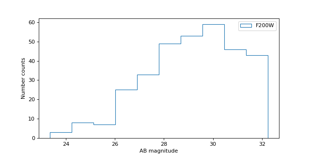
Plot number counts vs. magnitude

fig = plt.figure(figsize=(8, 4))

filt = 'F200W'
mag1 = tbl[filt + '_mag']

mag1 = mag1[(0 < mag1) & (mag1 < 90)]  # detections only
n = plt.hist(mag1, histtype='step', label=filt)

plt.xlabel('AB magnitude')
plt.ylabel('Number counts')
plt.legend()

<matplotlib.legend.Legend at 0x7f5c74919050>

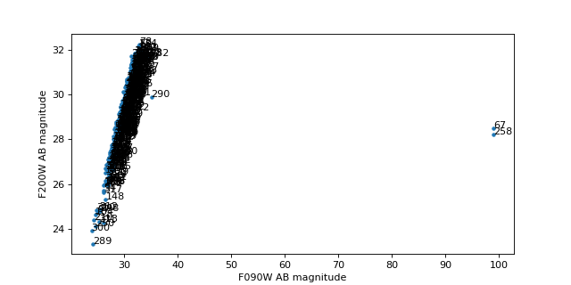
Plot F200W vs. F090W magnitudes and look for dropouts

#import mplcursors
# Would love a better solution here!

mag1 = tbl['F090W_mag']
mag2 = tbl['F200W_mag']

# Only plot detections in F200W
det2 = (0 < mag2) & (mag2 < 90)

mag1 = mag1[det2]
mag2 = mag2[det2]
ids = tbl['label'][det2]

plt.figure(figsize=(8, 4))

plt.plot(mag1, mag2, '.')

for i in range(len(mag1)):
    plt.text(mag1[i], mag2[i], ids[i])

plt.xlabel('F090W AB magnitude')
plt.ylabel('F200W AB magnitude')

Text(0, 0.5, 'F200W AB magnitude')

Look at one object

# Could select object by position
#x, y = 905, 276
#id = segm.data[y,x]

# Select by ID number
id = 261  # F090W dropout
obj = tbl[id-1]

obj

Row index=260

label	xcentroid	ycentroid	sky_centroid	area	a	b	ellipticity	orientation	gini	F090W_flux	F090W_fluxerr	F090W_mag	F090W_magerr	F115W_flux	F115W_fluxerr	F115W_mag	F115W_magerr	F150W_flux	F150W_fluxerr	F150W_mag	F150W_magerr	F200W_flux	F200W_fluxerr	F200W_mag	F200W_magerr	F277W_flux	F277W_fluxerr	F277W_mag	F277W_magerr	F335M_flux	F335M_fluxerr	F335M_mag	F335M_magerr	F356W_flux	F356W_fluxerr	F356W_mag	F356W_magerr	F410M_flux	F410M_fluxerr	F410M_mag	F410M_magerr	F444W_flux	F444W_fluxerr	F444W_mag	F444W_magerr
			deg,deg	pix2	pix	pix		deg		nJy	nJy			nJy	nJy			nJy	nJy			nJy	nJy			nJy	nJy			nJy	nJy			nJy	nJy			nJy	nJy			nJy	nJy
int32	float64	float64	SkyCoord	float64	float64	float64	float64	float64	float64	float64	float64	float64	float64	float64	float64	float64	float64	float64	float64	float64	float64	float64	float64	float64	float64	float64	float64	float64	float64	float64	float64	float64	float64	float64	float64	float64	float64	float64	float64	float64	float64	float64	float64	float64	float64
261	713.6003231522444	868.2862731469344	53.17147927632734,-27.79815855888541	111.0	2.1957364237904744	1.871859861852015	0.14750247726881305	-17.338774337937068	0.546245283985238	83.210645372822	3.527254135588318	26.599552774088977	0.04507502616775405	84.18846432688923	2.587997491179074	26.586868530823118	0.032873376920099	84.42481646179198	3.054886353923348	26.583824687102044	0.038592934581143754	78.728836865202	3.131787729879179	26.659665411873668	0.04235304682595798	45.258779395038786	0.9397610471453727	27.260742907280413	0.022313544876442264	35.277809352747205	1.0051267218729336	27.53124597775305	0.03050203683042903	32.91303372370136	0.9126975788091346	27.60658021307747	0.02969819980754908	24.75353531926416	0.9197377117713978	27.915906915058187	0.039610013762955344	25.401315400116076	1.0402217740639617	27.887859482444238	0.043576230399079735

obj['ellipticity']

\[0.14750248 \; \mathrm{}\]

segmobj = segm.segments[segm.get_index(id)]
segmobj

<photutils.segmentation.core.Segment>
label: 261
slices: (slice(863, 874, None), slice(708, 720, None))
area: 111

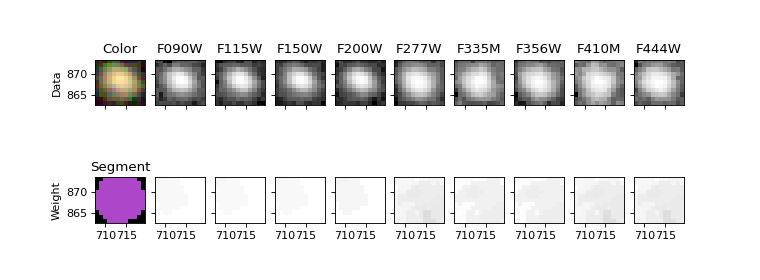
Show the object in all the images

fig, ax = plt.subplots(2, len(filters)+1, figsize=(9.5, 3.5), sharex=True, sharey=True)

ax[0, 0].imshow(rgb[segmobj.slices], origin='lower', extent=segmobj.bbox.extent)
ax[0, 0].set_title('Color')

cmap = segm.make_cmap(seed=12345)  # ERROR
ax[1, 0].imshow(segm.data[segmobj.slices], origin='lower', extent=segmobj.bbox.extent, cmap=cmap,
               interpolation='nearest')
ax[1, 0].set_title('Segment')

for i in range(1, len(filters)+1):
    filt = filters[i-1]

    # Show data on top row
    data = fits.open(imagefiles[filt])[0].data
    stamp = data[segmobj.slices]
    norm = ImageNormalize(stretch=SqrtStretch())  # scale each filter individually
    ax[0, i].imshow(stamp, extent=segmobj.bbox.extent, cmap='Greys_r', norm=norm, origin='lower')
    ax[0, i].set_title(filt.upper())

    # Show weights on bottom row
    weight = fits.open(weightfiles[filt])[0].data
    stamp = weight[segmobj.slices]
    # set black to zero weight (no exposure time / bad pixel)
    ax[1, i].imshow(stamp, extent=segmobj.bbox.extent, vmin=0, cmap='Greys_r', origin='lower')

ax[0, 0].set_ylabel('Data')
ax[1, 0].set_ylabel('Weight')

Text(0, 0.5, 'Weight')

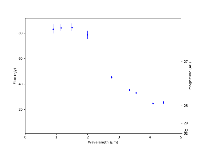
Plot SED (Spectral Energy Distribution)

fig, ax = plt.subplots(figsize=(8, 6))

for filt in filters:
    lam = int(filt[1:4]) / 100
    plt.errorbar(lam, obj[filt+'_flux'].value, obj[filt+'_fluxerr'].value, marker='.', c='b')

plt.axhline(0, c='k', ls=':')
plt.xlim(0, 5)
plt.xlabel('Wavelength ($\mu$m)')
plt.ylabel('Flux (nJy)')

mlim = 31.4
flim = mlim * u.ABmag
flim = flim.to(u.nJy).value

# Add AB magnitudes as secondary x-axis at right
# https://matplotlib.org/gallery/subplots_axes_and_figures/secondary_axis.html#sphx-glr-gallery-subplots-axes-and-figures-secondary-axis-py
def AB2nJy(mAB):
    m = mAB * u.ABmag
    f = m.to(u.nJy)
    f = f.value
    f = np.where(f > flim, f, flim)
    return f

def nJy2AB(F_nJy):
    f = F_nJy * u.nJy
    m = f.to(u.ABmag)
    m = m.value
    m = np.where(m < mlim, m, mlim)
    return m
    
plt.ylim(flim, plt.ylim()[1])

secax = ax.secondary_yaxis('right', functions=(nJy2AB, AB2nJy))
secax.set_ylabel('magnitude (AB)')

Text(0, 0.5, 'magnitude (AB)')

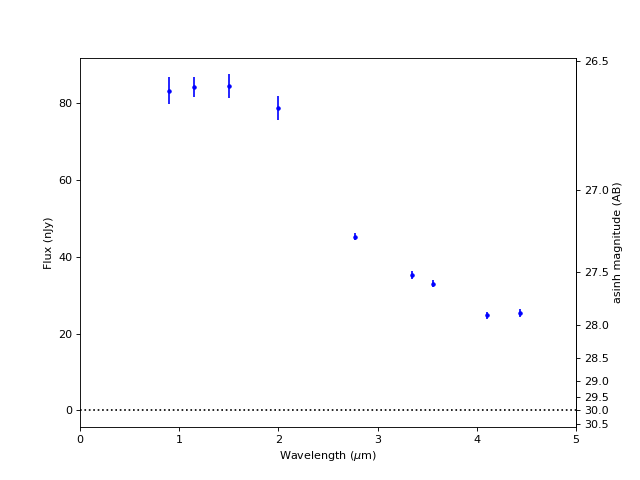
Magnitude conversion fails for flux <= 0

fig, ax = plt.subplots(figsize=(8, 6))

for filt in filters:
    lam = int(filt[1:4]) / 100
    plt.errorbar(lam, obj[filt+'_flux'].value, obj[filt+'_fluxerr'].value, marker='.', c='b')

plt.axhline(0, c='k', ls=':')
plt.xlim(0, 5)
plt.xlabel('Wavelength ($\mu$m)')
plt.ylabel('Flux (nJy)')

f0 = 10**(0.4 * 31.4)  # flux [nJy] at zero magnitude
b0 = 1.e-12  # this should be filter dependent

# Add AB magnitudes as secondary x-axis at right
# https://matplotlib.org/gallery/subplots_axes_and_figures/secondary_axis.html#sphx-glr-gallery-subplots-axes-and-figures-secondary-axis-py
def AB2nJy(m):
    f = np.sinh(-0.4 * m * np.log(10) - np.log(b0)) * 2 * b0 * f0
    return f

# Luptitudes
# https://www.sdss.org/dr12/algorithms/magnitudes/
def nJy2AB(f):
    m = -2.5 / np.log(10) * (np.arcsinh((f / f0) / (2 * b0)) + np.log(b0))
    return m

#plt.ylim(flim, plt.ylim()[1])

secax = ax.secondary_yaxis('right', functions=(nJy2AB, AB2nJy))
secax.set_ylabel('asinh magnitude (AB)')

Text(0, 0.5, 'asinh magnitude (AB)')