NIRSpec IFU Optimal Point Source Extraction#
This notebook illustrates various extraction methods for a point source in JWST NIRSpec IFU data, utilizing the Q3D (PID 1335) observation of quasar SDSS J165202.64+172852.3. The extraction techniques include subset extraction with Jdaviz, simple sum over spaxels, cylindrical aperture, conical aperture photometry, and optimal point source extraction using a WebbPSF model PSF.
Use case: optimal spectral extraction; method by Horne (1986). Data: JWST NIRSpec IFU data; point sources. Tools: jwst, webbpsf, matplotlib, scipy, custom functions. Cross-intrument: any spectrograph. Documentation: This notebook is part of a STScI’s larger post-pipeline Data Analysis Tools Ecosystem.
Table of Contents#
1. Imports #
numpy for array math
scipy for ndimage shift
specutils for Spectrum data model
jdaviz : for data visualization
photutils to define circular apertures
astropy.io for reading and writing FITS cubes and images
astropy.wcs, units, coordinates for defining and reading WCS
astropy.stats for sigma_clipping
astropy.utils for downloading files from URLs
matplotlib for plotting spectra and images
os for file management
astroquery.mast to download the data
import numpy as np
import scipy
from specutils import Spectrum
import jdaviz as jd
print("jdaviz Version={}".format(jd.__version__))
from photutils.aperture import CircularAperture, aperture_photometry
from astropy.io import fits
from astropy import wcs
from astropy import units as u
import os
from astroquery.mast import Observations
jdaviz Version=5.0.1
%matplotlib inline
import matplotlib.pyplot as plt
from matplotlib.colors import LogNorm
2. Read in NIRSpec IFU Cube #
The NIRSpec IFU observation of quasar SDSS J1652+1728 (redshift z=1.9) was taken using the G235H grating with F170LP filter, covering 1.66-3.17 microns at a spectral resolution of R~2700. The IFU spaxels are 0.1” on a side. The level-3 pipeline_processed datacube (s3d.fits, which combines all dithered exposures) is retrieved from MAST in the next notebook cell below.
# Download the data file
uri = "mast:jwst/product/jw01335-o008_t007_nirspec_g235h-f170lp_s3d.fits"
result = Observations.download_file(
uri, base_url="https://mast.stsci.edu/api/v0.1/Download/file"
)
if result[0] == "ERROR":
raise RuntimeError("Error retrieving file: " + result[1])
# Construct the local filepath
filename = os.path.join(os.path.abspath("."), uri.rsplit("/", 1)[-1])
# Optionally Replace MAST data with custom reprocessed data in the current directory
# filename="./jw01335-o008_t007_nirspec_g235h-f170lp_s3d.fits"
Downloading URL https://mast.stsci.edu/api/v0.1/Download/file?uri=mast:jwst/product/jw01335-o008_t007_nirspec_g235h-f170lp_s3d.fits to jw01335-o008_t007_nirspec_g235h-f170lp_s3d.fits ...
[Done]
# Open and inspect the file and WCS
with fits.open(filename, memmap=False) as hdulist:
sci = hdulist["SCI"].data
err = hdulist["ERR"].data
w = wcs.WCS(hdulist[1].header)
hdr = hdulist[1].header
print(w)
# Window the wavelength range to focus on Hbeta-[OIII]
spec1d = Spectrum.read(filename)
slice_range = range(500, 1100, 1)
wavelength = np.array(spec1d.spectral_axis.value)[slice_range[0]: slice_range[-1] + 1]
# List of cube slices for aperture photometry
sci_data = []
sci_var = []
for idx in slice_range:
sci_data.append(sci[idx, :, :])
sci_var.append(err[idx, :, :])
data = np.nan_to_num(np.array(sci_data))
var = np.array(sci_var)
print("\nTrimmed data shape:", data.shape)
WCS Keywords
Number of WCS axes: 3
CTYPE : 'RA---TAN' 'DEC--TAN' 'WAVE'
CUNIT : 'deg' 'deg' 'm'
CRVAL : -106.98898425200001 17.481222214 1.6601979666156693e-06
CRPIX : 22.0 20.0 1.0
PC1_1 PC1_2 PC1_3 : -1.0 0.0 0.0
PC2_1 PC2_2 PC2_3 : 0.0 1.0 0.0
PC3_1 PC3_2 PC3_3 : 0.0 0.0 1.0
CDELT : 2.77777781916989e-05 2.77777781916989e-05 3.95999988541007e-10
NAXIS : 43 39 3814
Trimmed data shape: (600, 39, 43)
jd1 = jd.new_app()
jd1.load(filename, format='3D Spectrum')
jd1.show()
# Set spectrum display limits
jd1.viewers['1D Spectrum'].set_limits(x_min = 1.65, x_max = 2.4, y_min=0.0, y_max=2e-9)
# Select slice to visualize
sli = jd1.plugins['Spectral Slice']
sli.value = 1.94 #microns
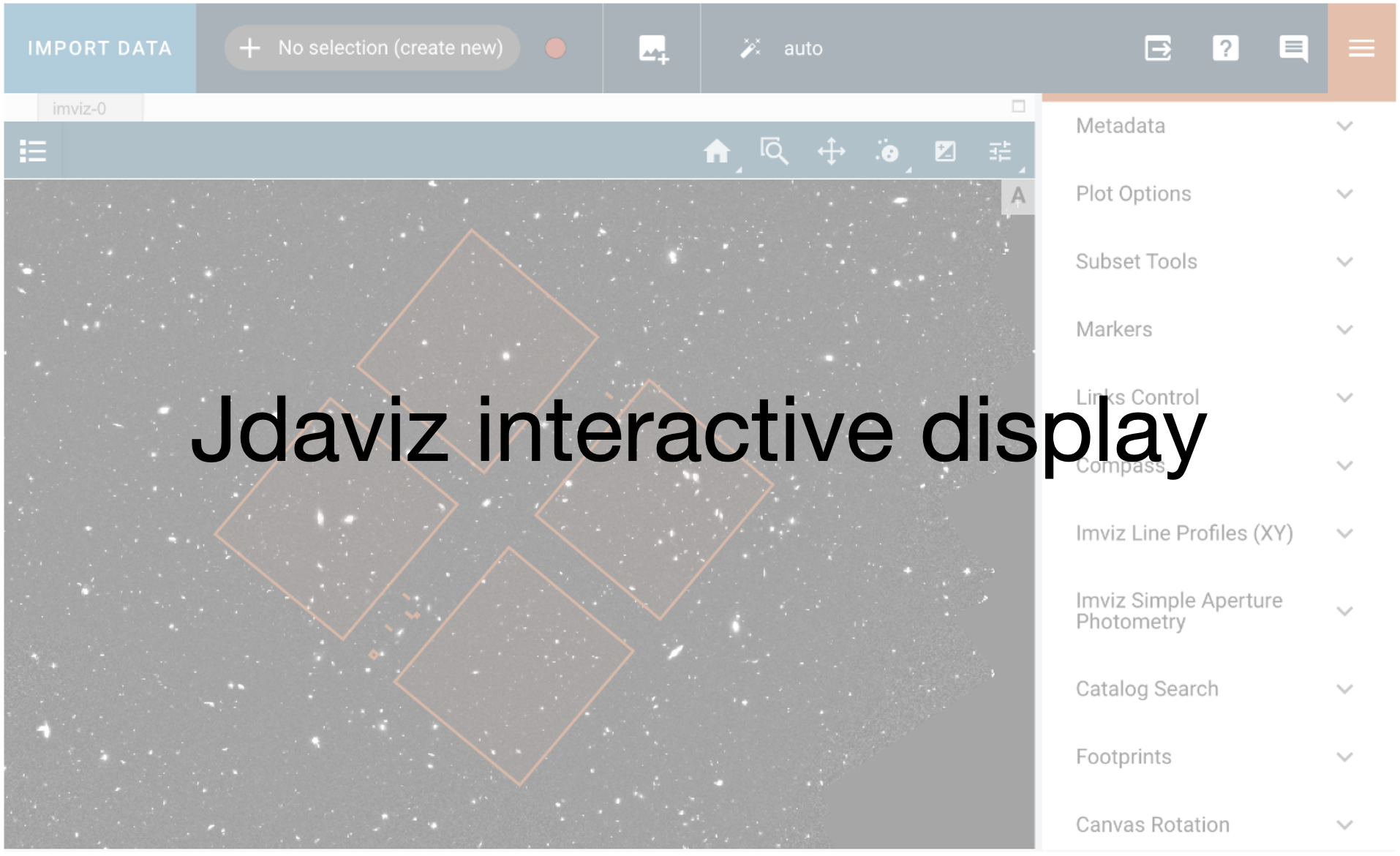
3. Visualize Science Data with Jdaviz #
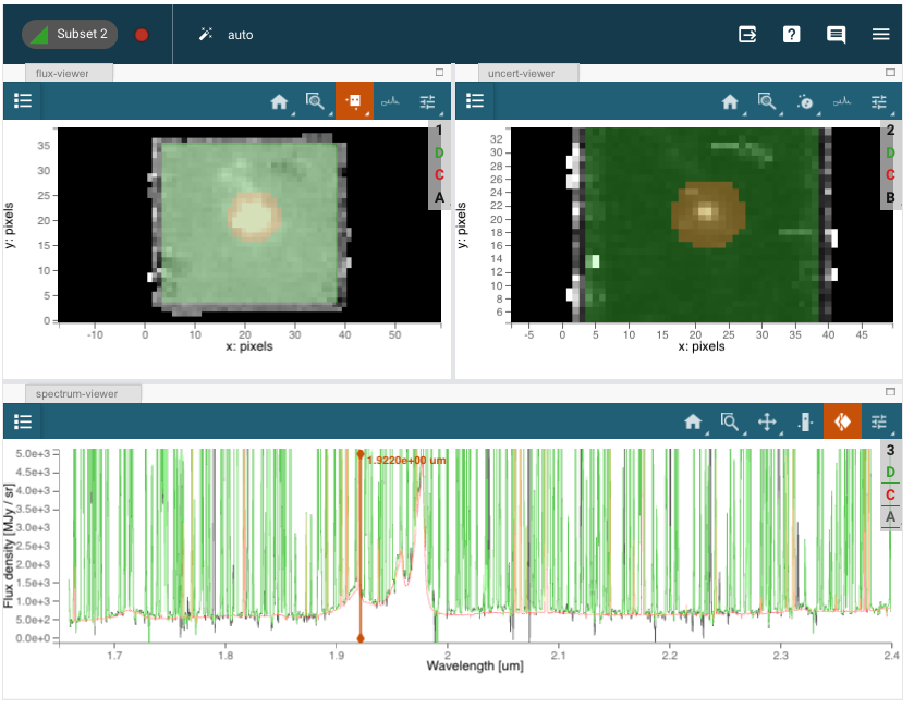
UI Instructions:#
Scrub through the cube to a line-free region using the spectrum-viewer slice tool.
In the flux-viewer, select one circular subset region centered on the quasar, and a square region to delimit the good area for spectral and background extraction
Note that the regions are pixelated and don’t include fractional pixels
The default collapse method is “Sum” in the spectrum viewer (see Plot Options:Line). “Median” may also be useful for visualization but will not give an accurate measurement of the total flux.)
4. Export Source and Good Data Regions from Jdaviz cube viewers #
Export the region defined by the user in Jdaviz as astropy PixelRegions
try:
print("\nSource Region")
region1 = jd.plugins['Subset Tools'].get_regions(region_type="spatial")['Subset 1']
print(region1)
center_xy = [region1.center.x, region1.center.y]
r_pix = region1.radius
region1_exists = True
except Exception:
print("There is no Subset 1 selected in the cube viewer.")
center_xy = [22.0, 21.0]
r_pix = 5.92
print("Using default pixel center and radius:")
print("Center pixel:", center_xy)
print("Radius (pixels):", r_pix)
region1_exists = False
print("\nGood Data Region")
try:
region2 = jd.plugins['Subset Tools'].get_regions(region_type="spatial")['Subset 2']
print(region2)
region2_exists = True
data_xrange = [
round(region2.center.x - region2.width / 2),
round(region2.center.x + region2.width / 2),
]
data_yrange = [
round(region2.center.y - region2.height / 2),
round(region2.center.y + region2.height / 2),
]
print("Good data (xmin,xmax), (ymin,ymax):", data_xrange, data_yrange)
good_data = np.nan_to_num(
data[:, data_yrange[0]: data_yrange[1], data_xrange[0]: data_xrange[1]]
)
good_var = var[:, data_yrange[0]: data_yrange[1], data_xrange[0]: data_xrange[1]]
except Exception:
print("There is no Subset 2 selected in the cube viewer.")
region1_exists = False
data_xrange = [7, 36]
data_yrange = [6, 33]
good_data = np.nan_to_num(
data[:, data_yrange[0]: data_yrange[1], data_xrange[0]: data_xrange[1]]
)
good_var = var[:, data_yrange[0]: data_yrange[1], data_xrange[0]: data_xrange[1]]
print("Using default good data (xmin,xmax), (ymin,ymax):", data_xrange, data_yrange)
Source Region
There is no Subset 1 selected in the cube viewer.
Using default pixel center and radius:
Center pixel: [22.0, 21.0]
Radius (pixels): 5.92
Good Data Region
There is no Subset 2 selected in the cube viewer.
Using default good data (xmin,xmax), (ymin,ymax): [7, 36] [6, 33]
5. Extract Subset Spectrum and Background from Jdaviz Spectrum Viewer #
Retrieve the collapsed spectrum (Subset1) of the user-defined region from the Spectrum Viewer as a Spectrum object.
subsets = jd.datasets
print(subsets.keys())
print("\nSource")
try:
spectrum_subset1 = jd.datasets['Spectrum (Subset 1, sum)'].get_data()
print(spectrum_subset1)
except Exception:
print("There is no Subset 1 selected in the spectrum viewer.")
print("\nBackground")
try:
spectrum_subset2 = jd.datasets['Spectrum (Subset 2, sum)'].get_data()
print(spectrum_subset2)
except Exception:
print("There is no Subset 2 selected in the spectrum viewer.")
dict_keys(['jw01335-o008_t007_nirspec_g235h-f170lp_s3d', 'jw01335-o008_t007_nirspec_g235h-f170lp_s3d [UNC]', 'jw01335-o008_t007_nirspec_g235h-f170lp_s3d (sum)', 'jw01335-o008_t007_nirspec_g235h-f170lp_s3d [DQ]'])
Source
There is no Subset 1 selected in the spectrum viewer.
Background
There is no Subset 2 selected in the spectrum viewer.
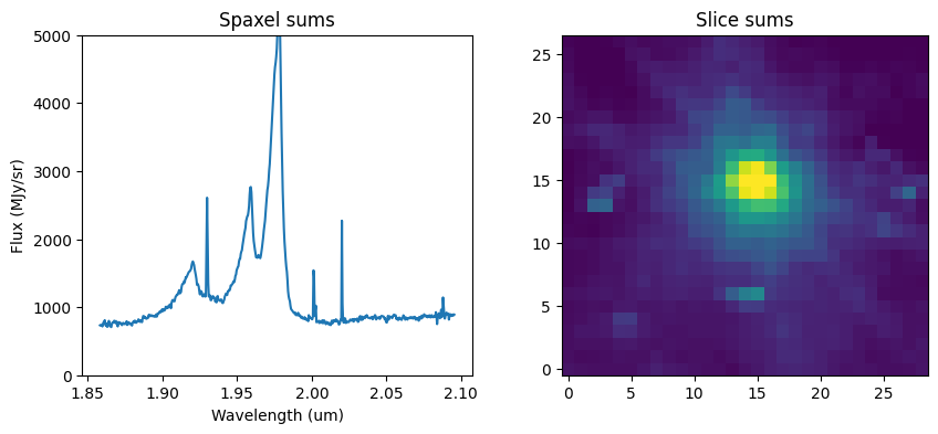
6. Extract Spectrum by Sum Over Spaxels #
Perform a simple numpy sum over all spaxels in the cube as a rudimentary extraction method. Also sum over wavelength to collapse the cube.
# Sum over wavelength
# Clip data for display purposes
clip_level = 4e4
data_clipped = np.clip(good_data, 0, clip_level)
cube_sum = np.sum(data_clipped, axis=0)
# Extraction via sum over spaxels
fnu_sum = np.sum(good_data, axis=(1, 2))
fnu_sum_clipped = np.clip(fnu_sum, 0, clip_level)
flux_spaxsum = np.array(fnu_sum) * u.MJy / u.sr
spec1d_spaxsum = Spectrum(spectral_axis=wavelength * u.um, flux=flux_spaxsum)
# Plots
f, (ax1, ax2) = plt.subplots(1, 2, figsize=(10, 4))
ax1.plot(wavelength, fnu_sum)
ax1.set_title("Spaxel sums")
ax1.set_xlabel("Wavelength (um)")
ax1.set_ylabel("Flux (MJy/sr)")
ax1.set_ylim(0, 5e3)
ax2.imshow(cube_sum, norm=LogNorm(vmin=100, vmax=clip_level), origin="lower")
ax2.set_title("Slice sums")
plt.show()
7. Extract Spectrum in Constant Radius Circular Aperture (Cylinder) #
This method is appropriate for an extended source.
# CircularAperture uses xy pixels
aperture = CircularAperture(center_xy, r=r_pix)
print(aperture)
cylinder_sum = []
for slice2d in data:
phot_table = aperture_photometry(slice2d, aperture)
cylinder_sum.append(phot_table["aperture_sum"][0])
flux_cylinder = np.array(cylinder_sum) * u.MJy / u.sr
spec1d_cylinder = Spectrum(spectral_axis=wavelength * u.um, flux=flux_cylinder)
Aperture: CircularAperture
positions: [22., 21.]
r: 5.92
8. Extract Spectrum in Linearly Expanding Circular Aperture (Cone) #
This method is appropriate for a point source PSF with width proportional to wavelength
# Reference wavelength for expanding aperture
lambda0 = wavelength[0]
print("Reference wavelength:", lambda0)
cone_sum = []
idx = -1
for (slice2d, wave) in zip(data, wavelength):
idx = idx + 1
r_cone = r_pix * wave / lambda0
aperture_cone = CircularAperture(center_xy, r=r_cone)
phot_table = aperture_photometry(
slice2d, aperture_cone, wcs=w.celestial, method="exact"
)
cone_sum.append(phot_table["aperture_sum"][0])
flux_cone = np.array(cone_sum) * u.MJy / u.sr
spec1d_cone = Spectrum(spectral_axis=wavelength * u.um, flux=flux_cone)
Reference wavelength: 1.858197960886173
9. Plot and Compare Non-optimal Spectral Extractions #
Compare spectra extracted in cylinder and cone subsets.
f, (ax1) = plt.subplots(1, 1, figsize=(15, 5))
# ax1.plot(wavelength, flux_spaxsum.value, label="All spaxels", c='k')
ax1.plot(wavelength, flux_cylinder.value, label="Cylinder", c="b")
ax1.plot(wavelength, flux_cone.value, label="Cone", c="darkorange", alpha=0.5)
try:
ax1.plot(
wavelength,
spectrum_subset1.flux.value[slice_range[0]: slice_range[-1] + 1],
c="r",
label="Subset1",
alpha=0.4,
)
except Exception:
print("There is no Subset1 spectrum to plot.")
ax1.set_title("Non-optimal spectral extractions")
ax1.set_xlabel("Observed Wavelength (microns)")
ax1.set_ylabel("Flux Density")
ax1.set_ylim(0, 5.0e3)
ax1.legend()
plt.show()
There is no Subset1 spectrum to plot.
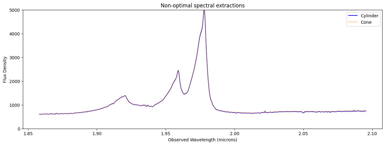
The non-optimal cylindrical, conical, and Jdaviz subset spectral extractions are quite similar. The conical extraction captures more flux at long wavelengths. Red-shifted Broad H-beta and narrow [O III] lines are visible in the quasar spectra.
10. WebbPSF Model PSF for Optimal Extraction #
Generate PSF model cube using WebbPSF for NIRSpec IFU, or read in precomputed PSF model cube.
WebbPSF installation instructions can be found in ReadTheDocs.
Caution! The WebbPSF model takes about 10 hr to run. Uncomment the following cell to do so. Otherwise, read in the precomputed WebbPSF model, which covers the full wavelength range of the present NIRSpec G235H dataset. For other filter/grating combinations, uncomment and run the cell below using the wavelengths from the science data set.
# #WebbPSF imports
# %pylab inline
# import webbpsf
#
# #WebbPSF commands used to create PSF model cube
# ns = webbpsf.NIRSpec()
# ns.image_mask = "IFU" # Sets to 3x3 arcsec square mask
# wavelengths = wavelength*1.0E-6
# psfcube = ns.calc_datacube(wavelengths, fov_pixels=30, oversample=4, add_distortion=True)
# psfcube.writeto("Webbpsf_ifucube.fits")
BoxPath = "https://data.science.stsci.edu/redirect/JWST/jwst-data_analysis_tools/IFU_optimal_extraction/"
psf_filename = BoxPath + "Webbpsf_ifucube.fits"
# Open WebbPSF data cube
with fits.open(psf_filename, memmap=False) as hdulist:
psf_model = hdulist["DET_SAMP"].data
psf_hdr = hdulist["DET_SAMP"].header
hdulist.info()
# Pad PSF model cube with zeros to match the present dataset
# (Different padding may be needed for your particular dataset)
print(sci.shape, psf_model.shape)
psf_model_padded = np.pad(psf_model, ((0, 0), (4, 5), (6, 7)), "constant")
# Sum over wavelength
psf_model_sum = np.sum(psf_model_padded[slice_range[0]: slice_range[-1] + 1], axis=0)
# Sum over spaxels
psf_model_fnusum = np.sum(
psf_model_padded[slice_range[0]: slice_range[-1] + 1], axis=(1, 2)
)
Filename: /home/runner/.astropy/cache/download/url/4931b72fec159f8a439e8c80c181370f/contents
No. Name Ver Type Cards Dimensions Format
0 OVERSAMP 1 PrimaryHDU 105786 (120, 120, 3915) float64
1 DET_SAMP 1 ImageHDU 105788 (30, 30, 3915) float64
2 OVERDIST 1 ImageHDU 105831 (120, 120, 3915) float64
3 DET_DIST 1 ImageHDU 105832 (30, 30, 3915) float64
(3814, 39, 43) (3915, 30, 30)
11. Align Model PSF Cube with Science Data #
Flip, smooth, and shift the model PSF cube to align with the simulated data. Trim the simulated data.
Important Note 1: this PSF will likely be rotated with respect to your dataset, depending on telescope roll angle. You can either rotate it to match your data or reprocess your data using the ifualign keyword to align the WCS with the instrumental coordinate frame.
Important Note 2: this PSF will likely be shifted with respect to your dataset. It would be beneficial to automatically find the (x,y) offset between the data and simulated PSF peaks. Currently the shift is determined empirically by eye.
# Flip model PSF left-right to match data.
psf_model_fliplr = psf_model_padded[:, ::-1, :]
# Empirically (chi-by-eye) determined shift
shiftx = 1.5 # 2
shifty = 1.5 # 1.5
# Shift model PSF using linear interpolation
psf_model_aligned = scipy.ndimage.shift(
psf_model_fliplr,
(0.0, shiftx, shifty),
order=1,
mode="constant",
cval=0.0,
prefilter=True,
)
good_psf_model = psf_model_aligned[
slice_range[0]: slice_range[-1] + 1,
data_yrange[0]: data_yrange[1],
data_xrange[0]: data_xrange[1],
]
# Sum over wavelength
psf_model_sum = np.sum(good_psf_model, axis=0)
# Scale factor for PSF subtraction
psf_sum_max = np.amax(psf_model_sum)
scalefactor = np.amax(cube_sum) / psf_sum_max
# Plots
f, ([ax1, ax2], [ax3, ax4]) = plt.subplots(2, 2, figsize=(10, 10))
ax1.set_title("PSF slice sum")
ax1.imshow(psf_model_sum, norm=LogNorm(), origin="lower")
ax2.set_title("Science Data slice sum")
ax2.imshow(cube_sum, norm=LogNorm(), origin="lower")
ax3.set_title("Data / PSF Ratio")
ax3.imshow(cube_sum / psf_model_sum, norm=LogNorm(vmin=1, vmax=1e6), origin="lower")
im4 = ax4.imshow(
np.log10(np.absolute(cube_sum - 0.75 * scalefactor * psf_model_sum)), origin="lower"
)
plt.colorbar(im4)
ax4.set_title("log abs(Data - PSF)")
plt.show()
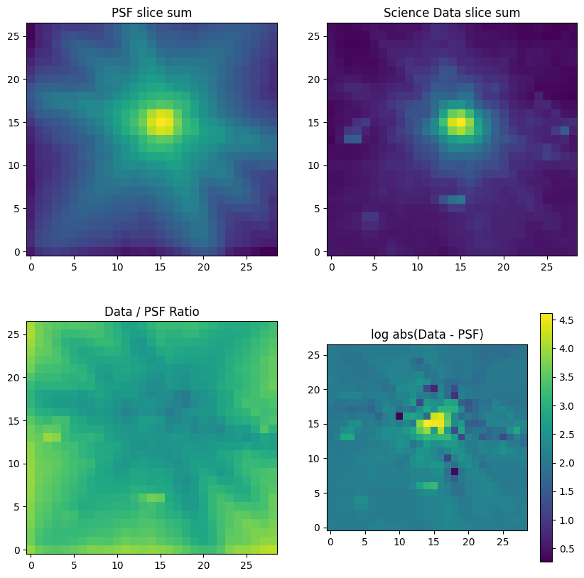
Figure top row: Comparison of shifted WebbPSF PSF (left) to science data (right). The NIRSpec IFU PSF is signficantly different from the WebbPSF simulation for the telescope. This is partly due to the IFU optics and perhaps partly due to the cube building algorithm. There is also some real extended emission from the QSO host and surrounding galaies.
Figure bottom row: Differences between the model PSF and the observed PSF will result in a sub-optimal extraction, not quite attaining the maximum SNR, but still better than a sum over all spaxels.
12. Optimal Extraction using WebbPSF Model #
Optimal extraction (Horne 1986, PASP, 98, 609) weights the flux contributions to a spectrum by their signal-to-noise ratio (SNR). Dividing the simulated data by the model PSF gives an estimate of the total flux density spectrum in each spaxel. A weighted average of these estimates over all spaxels yields the optimally extracted spectrum over the cube. In the faint source limit, where the noise is background-dominated, optimal extraction inside a 3-sigma radius can increase the effective exposure time by a factor of 1.69 (Horne et al. 1986). In the bright source limit, where the noise is dominated by the Poisson statistics of the source, optimal extraction is formally identical to a straight sum over spaxels for a perfect PSF model.
We use the precomputed WebbPSF PSF model for optimal extraction here.
# Window PSF model (and replace NaNs)
good_profile = np.nan_to_num(good_psf_model)
var_clean = np.nan_to_num(good_var, nan=1e12, posinf=1e12, neginf=1e12)
zerovar = np.where(var_clean == 0)
var_clean[zerovar] = 1e12
var_clean_sum = np.sum(var_clean, axis=(0))
snr_clean = np.nan_to_num(good_data / var_clean)
# Divide data by PSF model
data_norm = np.nan_to_num(good_data / good_profile, posinf=0, neginf=0)
data_norm_sum = np.sum(data_norm, axis=0)
# Mask out bad data
# data_norm_clipped = sigma_clip(data_norm, sigma=3.0, maxiters=5, axis=(1, 2))
data_norm_clipped = data_norm
data_norm_clipped_sum = np.sum(data_norm_clipped, axis=0)
snr_thresh = 1.0
badvoxel = np.where((data_norm_clipped == 0) | (snr_clean < snr_thresh))
data_clean = 1.0 * good_data
data_clean[badvoxel] = 0.0
data_clean_sum = np.sum(data_clean, axis=0)
# Optimal extraction, using model profile weight and variance cube from the simulated data
optimal_weight = np.nan_to_num(
good_profile**2 / var_clean, posinf=0, neginf=0
) # Replace nans and infs with 0
optimal_weight_sum = np.sum(optimal_weight, axis=(0))
optimal_weight_norm = np.sum(optimal_weight, axis=(1, 2))
spectrum_optimal = (
np.sum(good_profile * data_clean / var_clean, axis=(1, 2)) / optimal_weight_norm
)
# Plots
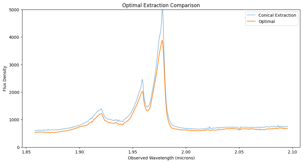
f, (ax1) = plt.subplots(1, 1, figsize=(12, 6))
ax1.set_title("Optimal Extraction Comparison")
ax1.set_xlabel("Observed Wavelength (microns)")
ax1.set_ylabel("Flux Density")
ax1.set_ylim(0, 5000)
ax1.plot(wavelength, cone_sum, label="Conical Extraction", alpha=0.5)
ax1.plot(wavelength, spectrum_optimal, label="Optimal")
ax1.legend()
plt.show()
# create a new instance of jdaviz
jd_2 = jd.new_app()
flux_opt = spectrum_optimal * u.MJy / u.sr
spec1d_opt = Spectrum(spectral_axis=wavelength * u.um, flux=flux_opt)
# jd_2.load_data(spec1d_spaxsum, data_label="collapse spec")
jd_2.load(spec1d_opt, format='1D Spectrum', data_label="optimal spec")
jd_2.load(spec1d_cone, format='1D Spectrum', data_label="cone spec")
jd_2.show()
# set spectrum display limits
jd.plugins['Plot Options'].y_min = 0.0
jd.plugins['Plot Options'].y_max = clip_level / 7
# jd_2.y_limits(0.0, clip_level / 7)
The viewer looks like this:
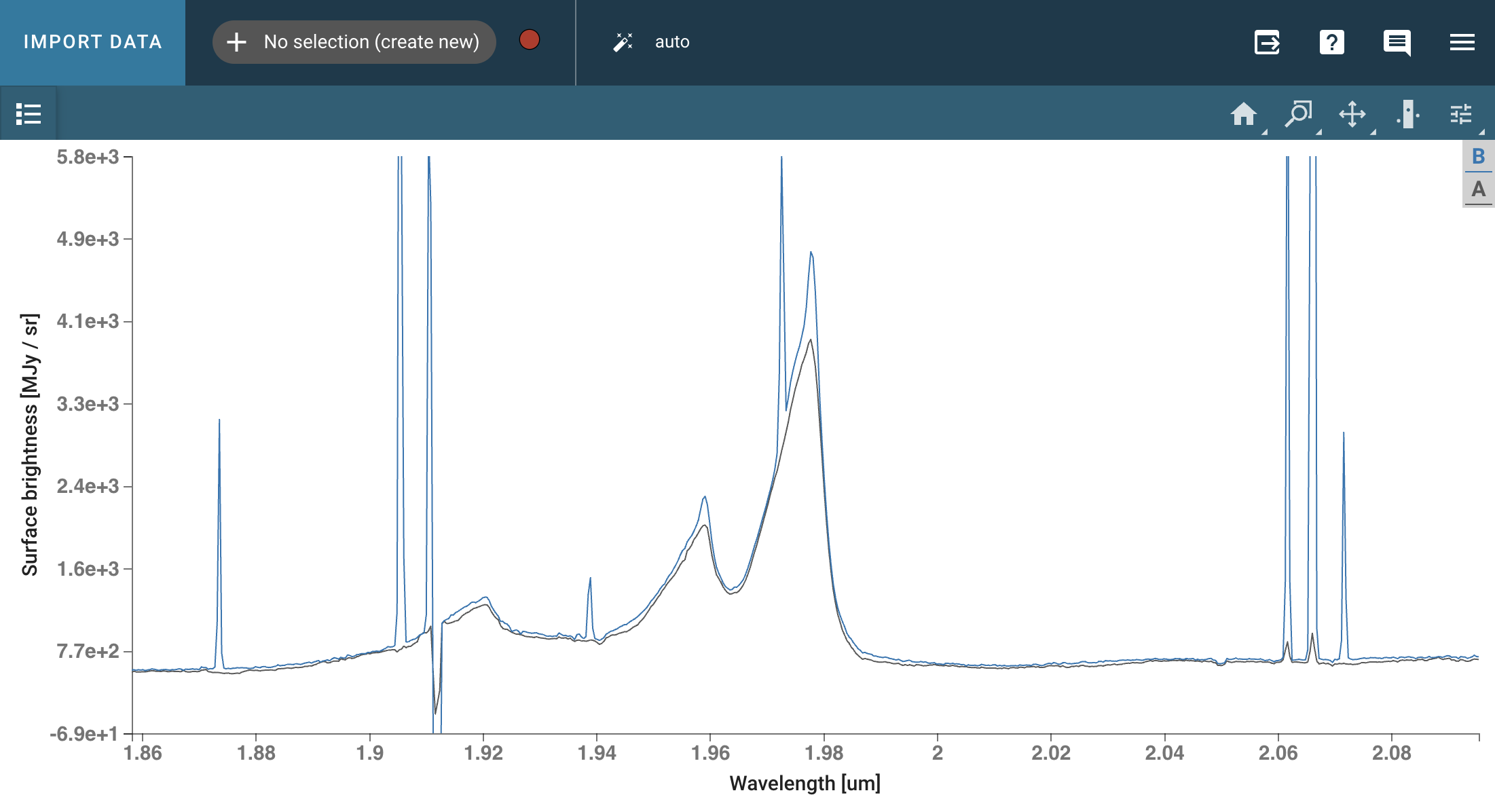
The optimally extracted spectrum is less noisy than the aperture extraction and incorporates fewer bad pixels and cosmic ray events. The OIII line profile is different because extended emission is downweighted with respect to the unresolved quasar nucleus.

Notebook created by Patrick Ogle and James Davies. Last update: May 2026.