MOS Spectroscopy of Extragalactic Field#
Use case: emission-line measurements and template matching on 1D spectra.
Data: CEERS NIRSpec observations
Tools: specutils, astropy, matplotlib, jdaviz.
Cross-intrument:
Documentation: This notebook is part of a STScI’s larger post-pipeline Data Analysis Tools Ecosystem.
Introduction#
In this notebook, we will inspect a set of spectra and perform a seris of spectroscopic analyses on an example spectrum, including continuum fitting and subtraction, line identification, centroiding and flux measurements, gaussian fitting, equivalent widths, and template fitting. We will do so using the interactive jdaviz package and the command line. We will use a JWST/NIRSpec spectroscopic dataset from the CEERS program.
Objective of the notebook#
The aim of the notebook is to showcase how to use the visualization tool Jdaviz or the combination Specutils+Matplotlib to measure the properties of the OII emission line in a NIRSpec spectrum.
Workflow#
visualize the spectroscopic dataset in Mosviz
select one galaxy (s02904) and visualize it in Jdaviz
perform the 1D extraction of the bright companion using the Spectral Extraction plugin in Jdaviz
attach the wavelength axis to the extracted 1D spectrum
select the OII emission line and measure
the redshift of the source
the properties of the emission line
fit a model with continuum + a Gaussian to the OII emission line
perform the same tasks using Specutils and Matplotlib instead of Jdaviz
find the best-fitting template of the observed spectrum
System requirements#
First, we create an environment with jdaviz which contains all the spectroscopic packages we need.
conda create -n jdaviz python
conda activate jdaviz
pip install jdaviz
Imports#
# general os
import zipfile
import urllib.request
from pathlib import Path
# general plotting
from matplotlib import pyplot as plt
# table/math handling
import numpy as np
# astropy
import astropy
import astropy.units as u
from astropy.io import fits, ascii
from astropy.nddata import StdDevUncertainty
from astropy.modeling import models
from astropy.visualization import quantity_support
# specutils
import specutils
from specutils import Spectrum, SpectralRegion
from specutils.fitting import fit_generic_continuum
from specutils.fitting import find_lines_threshold
from specutils.fitting import fit_lines
from specutils.manipulation import extract_region
from specutils.analysis import centroid
from specutils.analysis import line_flux
from specutils.analysis import equivalent_width
from specutils.analysis import template_comparison
# jdaviz
import jdaviz
import jdaviz as jd
from jdaviz import Mosviz
np.seterr(all='ignore') # hides irrelevant warnings about divide-by-zero, etc
quantity_support() # auto-recognizes units on matplotlib plots
# Matplotlib parameters
params = {'legend.fontsize': '18',
'axes.labelsize': '18',
'axes.titlesize': '18',
'xtick.labelsize': '18',
'ytick.labelsize': '18',
'lines.linewidth': 2,
'axes.linewidth': 2,
'animation.html': 'html5'}
plt.rcParams.update(params)
plt.rcParams.update({'figure.max_open_warning': 0})
Check versions. Latest working environment is:#
Numpy: 2.1.0
Astropy: 7.0.1
Specutils: 1.19.0
Jdaviz: 5.0.0
print("Numpy: ", np.__version__)
print("Astropy: ", astropy.__version__)
print("Specutils: ", specutils.__version__)
print("Jdaviz: ", jdaviz.__version__)
Numpy: 2.4.6
Astropy: 7.2.0
Specutils: 2.3.0
Jdaviz: 5.0.1
Set path to data and download from box link#
# Download the data from the old version of this notebook. They include the templates for fitting
boxlink = 'https://data.science.stsci.edu/redirect/JWST/jwst-data_analysis_tools/mos_spectroscopy/mos_spectroscopy.zip'
boxfile = Path('./mos_spectroscopy.zip')
urllib.request.urlretrieve(boxlink, boxfile)
zf = zipfile.ZipFile(boxfile, 'r')
zf.extractall()
# Download the s2d and x1d files
boxlink_ceers = 'https://data.science.stsci.edu/redirect/JWST/jwst-data_analysis_tools/mos_spectroscopy/mos_ceers_data.zip'
boxfile_ceers = Path('./mos_ceers_data.zip')
urllib.request.urlretrieve(boxlink_ceers, boxfile_ceers)
zf = zipfile.ZipFile(boxfile_ceers, 'r')
zf.extractall()
Developer note:
The download of JWST data could happen directly from MAST, but the observations are organized in separate folders, while Mosviz wants the data in a single folder. So we go with a box download.
pathtodata = Path('./data')
Open data in Mosviz#
In Mosviz we can explore all the data products in the folder. This cell takes a minute or two to run. Since we are not including images, we can expand the 2D/1D spectra viewers to use the full width of the GUI. We can also keep the plugin tray open on metadata to check specifics of the files we are looking at.
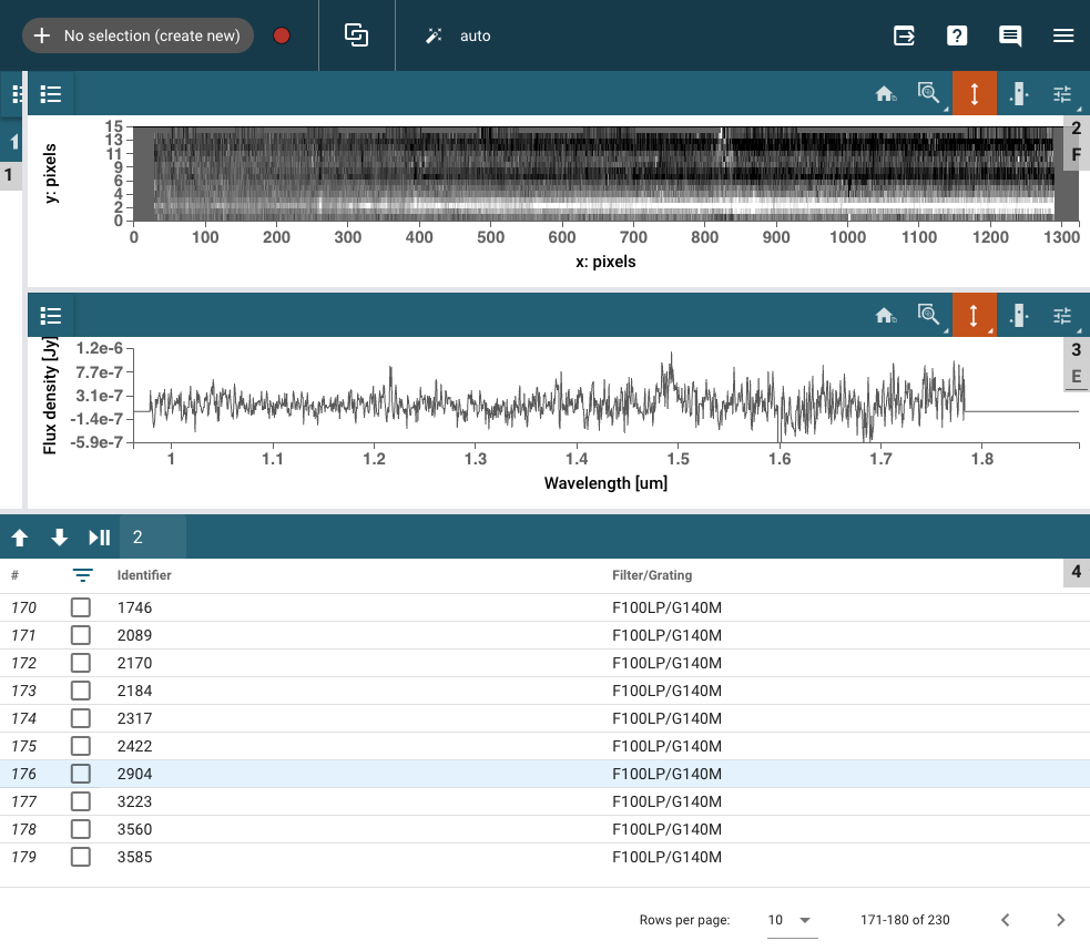
Choose one galaxy#
We choose s02904 because we want to extract the very bright companion below the target.
file1d = pathtodata / 'jw01345-o064_s02904_nirspec_f100lp-g140m_x1d.fits'
file2d = pathtodata / 'jw01345-o064_s02904_nirspec_f100lp-g140m_s2d.fits'
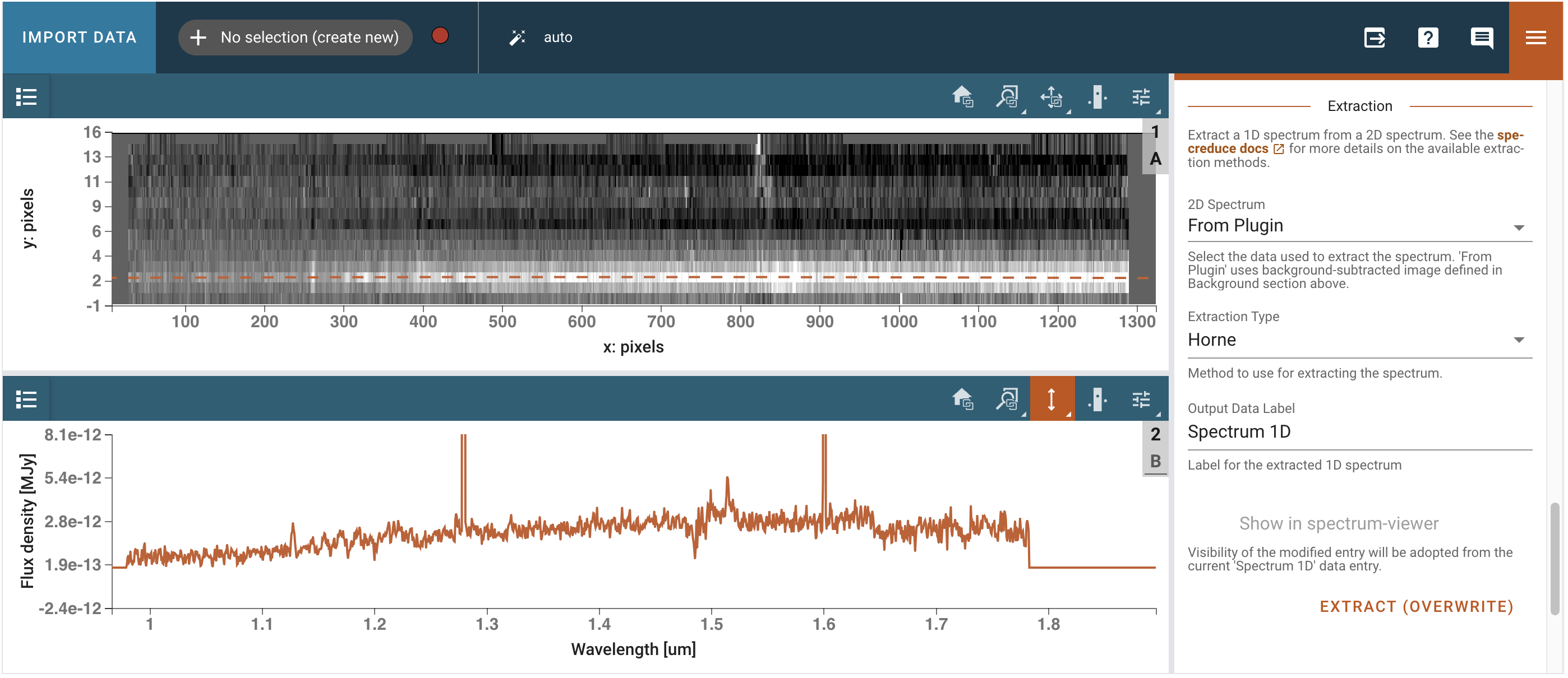
Use Jdaviz to extract a better 1D spectrum#
specviz2d = jd.new_app()
specviz2d.load(file2d, format='2D Spectrum')
specviz2d.show()
ylims = specviz2d.plugins['Plot Options']
ylims.viewer = '1D Spectrum'
ylims.y_max = 8e-12
Developer note
Is there a way to get out an uncertainty array from the extraction?
This is being worked on.
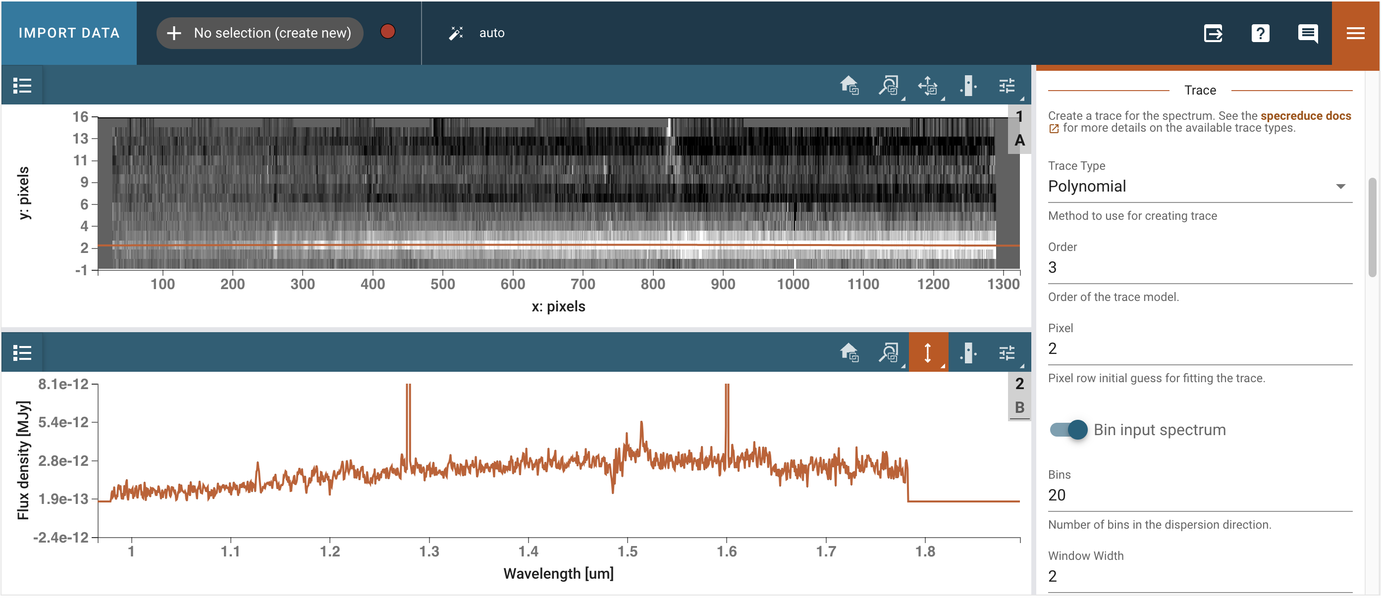
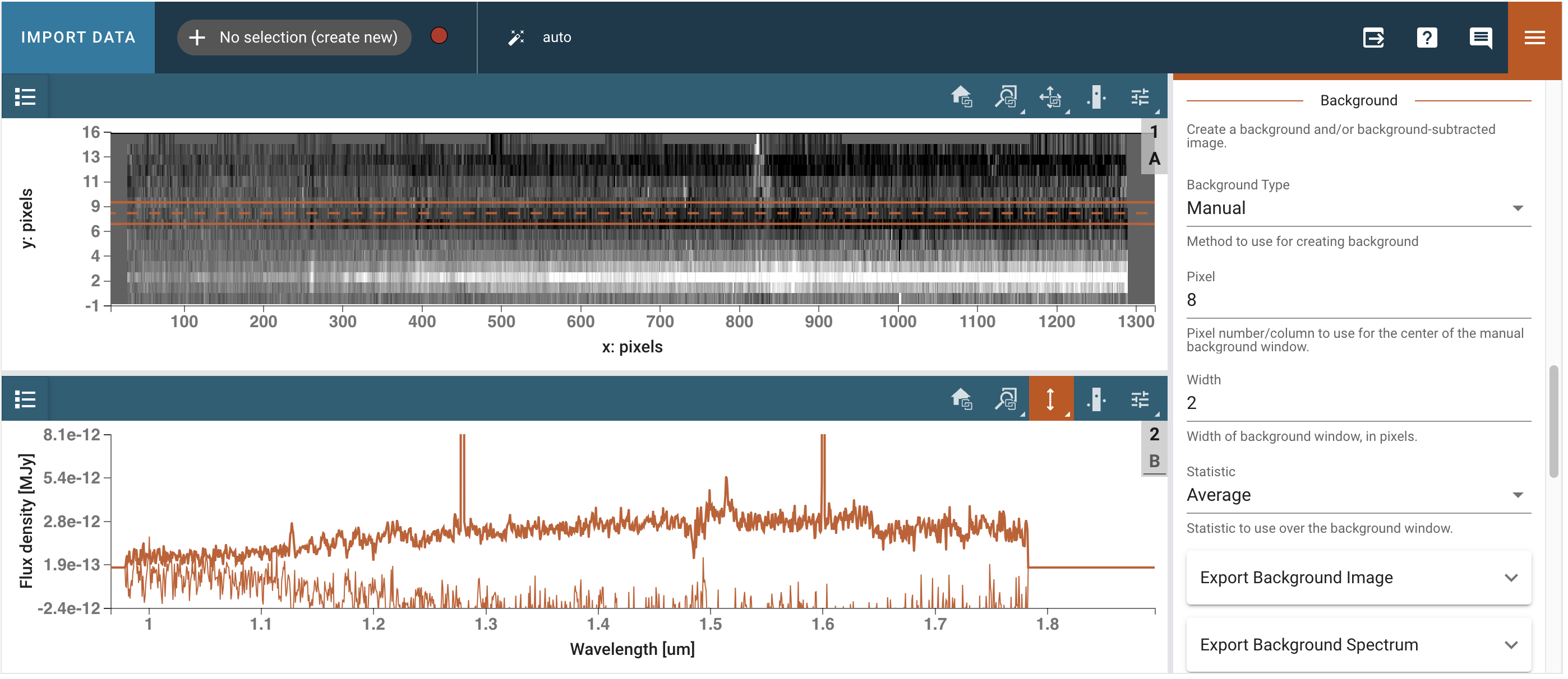
We open the 2D Spectral Extraction plugin and select the appropriate trace (Polynomial, order 3, on pixel 2), background (Manual, on pixel 8, width 2, statistic average), and extraction (From Plugin, Horne, label: ‘1D ext Spectrum’). We then click Extract and inspect the extracted spectrum in the 1D viewer.
# using API calls, we can perform the 1D spectral extraction
extract = specviz2d.plugins['2D Spectral Extraction']
extract.keep_active = True
# trace
extract.trace_type = 'Polynomial'
extract.trace_order = 3
extract.trace_pixel = 2
# background
extract.bg_type = 'Manual'
extract.bg_trace_pixel = 8
extract.bg_width = 2
extract.bg_statistic = 'Average'
# extraction
extract.ext_dataset = 'From Plugin'
extract.ext_type = 'Horne'
extract.ext_add_results.label = '1D ext Spectrum'
extract.ext_add_results.viewer = '1D Spectrum'
# extract spectrum
extract.export_extract_spectrum(add_data=True)
<Spectrum(flux=[nan ... nan] MJy (shape=(1325,), mean=0.00000 MJy); spectral_axis=<SpectralAxis
(observer to target:
radial_velocity=0.0 km / s
redshift=0.0)
[0.000e+00 1.000e+00 2.000e+00 ... 1.322e+03 1.323e+03 1.324e+03] pix> (length=1325); uncertainty=StdDevUncertainty)>
# Get out extracted spectrum from Jdaviz
spectra = specviz2d.datasets['1D ext Spectrum'].get_data()
spectra
<Spectrum(flux=[nan ... nan] MJy (shape=(1325,), mean=0.00000 MJy); spectral_axis=<SpectralAxis [0.000e+00 1.000e+00 2.000e+00 ... 1.322e+03 1.323e+03 1.324e+03] pix> (length=1325); uncertainty=StdDevUncertainty)>
# developer: Need to confirm how to automate adding in spectral axis
# add a spectral axis using the spectral axis taken from mosviz.
xwave = np.linspace(0.96251938, 1.89576744, 1471)[0:1325]*u.um
# Include some fake uncertainty for now
spec1d = Spectrum(spectral_axis=xwave,
flux=spectra.flux,
uncertainty=StdDevUncertainty((np.zeros(len(spectra.flux)) + 1E-13) * spectra.unit))
spec1d
<Spectrum(flux=[nan ... nan] MJy (shape=(1325,), mean=0.00000 MJy); spectral_axis=<SpectralAxis [0.96251938 0.96315424 0.96378911 ... 1.80180777 1.80244263 1.8030775 ] um> (length=1325); uncertainty=StdDevUncertainty)>
# And open in Jdaviz
specviz = jd.new_app()
specviz.load(spec1d, format = '1D Spectrum', data_label='spec1d calibrated')
specviz.plugins['Plot Options'].y_max = 2.1e-11
specviz.show()
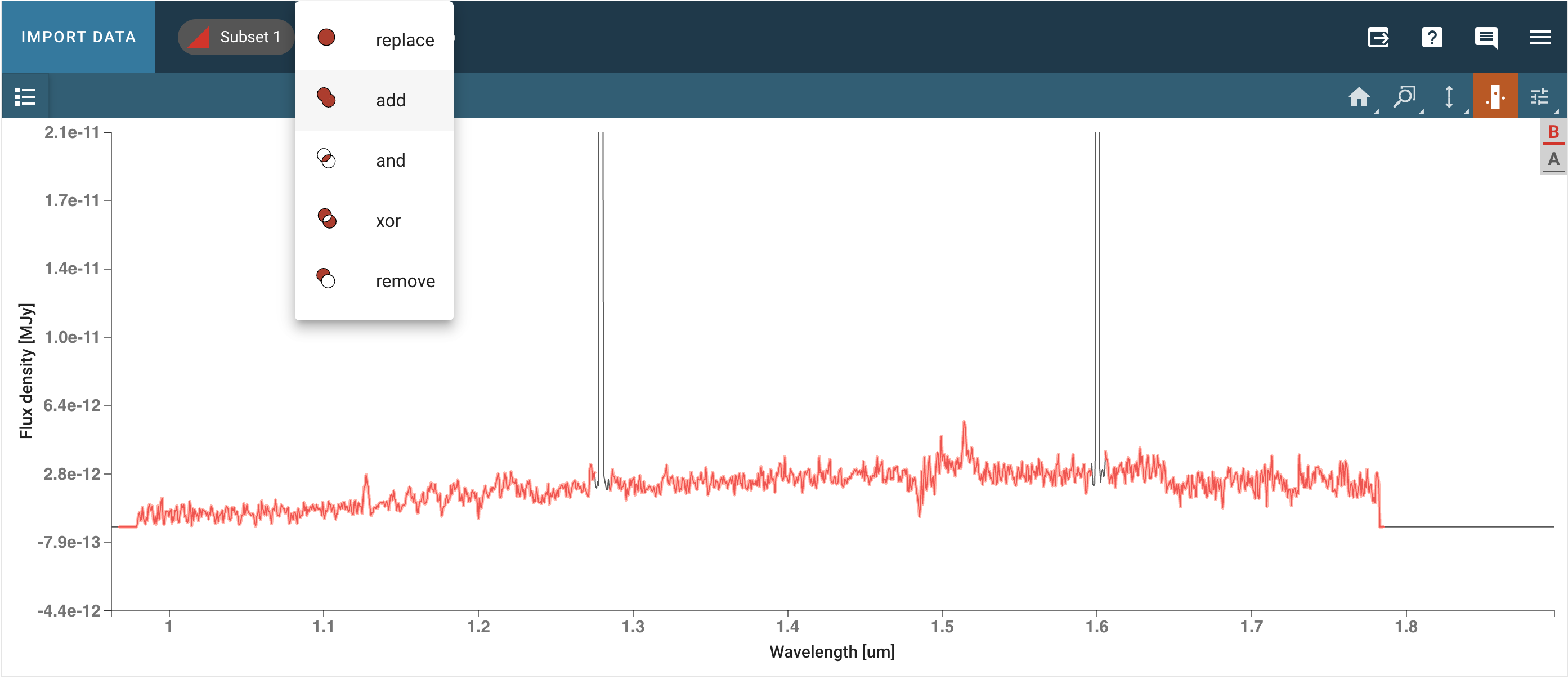
There are still some artifacts in the data, but we can select a subset masking the artifacts and get out a spectrum without unwanted spikes. We can do so using the tool to select a subset with the “add” option (click the red circle and select ‘add’) to select multiple regions as part of a single subset.
# Create a subset in the area of interest if it has not been created manually
plg_sub = specviz.plugins['Subset Tools']
region1 = plg_sub.get_regions()
if len(region1) == 0:
print("There are no subsets selected.")
region1_exists = False
else:
region1_exists = True
# Spectral region for masking artifacts just around [OII]
if not region1_exists:
region1 = SpectralRegion(1.*u.um, 1.27*u.um)
plg_sub.import_region(region1)
print("Subset 1 created")
There are no subsets selected.
Subset 1 created
# Get spectrum out with mask
spec1d_region = plg_sub.get_regions()
print(spec1d_region)
spec1d_masked = extract_region(spec1d, spec1d_region['Subset 1'], return_single_spectrum=True)
{'Subset 1': Spectral Region, 1 sub-regions:
(1.0 um, 1.27 um) }
# Load in jdaviz
specviz.load(spec1d_masked, format='1D Spectrum', data_label='spec1d masked')
# Write the extracted spectrum to a fits file
file_extracted = Path('./extracted_spectrum.fits')
spec1d_masked.write(file_extracted, overwrite=True)
# Check that it has everything
hdu = fits.open(file_extracted)
hdu.info()
Filename: extracted_spectrum.fits
No. Name Ver Type Cards Dimensions Format
0 PRIMARY 1 PrimaryHDU 4 ()
1 DATA 1 BinTableHDU 20 425R x 4C [D, D, D, L]
Workflow via API calls#
I can do some analysis on the spectrum using the plugins in the GUI. For reproducibility, I can do the same thing from the API, changing the parameters in the plugins programmatically.
Select regions#
# Select two regions in the spectrum
region_line = SpectralRegion(1.124*u.um, 1.131*u.um)
region_line_con = SpectralRegion(1.05*u.um, 1.25*u.um)
# Send the regions to jdaviz
plg_sub.import_region(region_line, combination_mode='new')
plg_sub.import_region(region_line_con, combination_mode='new')
Line analysis#
![Jdaviz showing the region on the [OII] line and the line analysis plugin.](../../../_images/line_analysis.png)
# Open line analysis plugin
plugin_la = specviz.plugins['Line Analysis']
plugin_la.open_in_tray()
# List what's in the data menu
specviz.datasets.keys()
dict_keys(['spec1d calibrated', 'spec1d masked'])
# Input the appropriate spectrum and region
plugin_la.dataset = 'spec1d masked'
plugin_la.spectral_subset = 'Subset 2'
# Input the values for the continuum
plugin_la.continuum = 'Surrounding'
plugin_la.continuum_width = 7
# Return line analysis results
plugin_la.get_results()
[{'function': 'Line Flux',
'result': '1.4261880658716583e-20',
'uncertainty': '4.964844660366441e-22',
'unit': 'W / m2'},
{'function': 'Equivalent Width',
'result': '-0.004960716760249802',
'uncertainty': '0.0005777682064911259',
'unit': 'um'},
{'function': 'Gaussian Sigma Width',
'result': '0.0009493315105240565',
'uncertainty': '0.00012573704674734393',
'unit': 'um'},
{'function': 'Gaussian FWHM',
'result': '0.0022355048703615577',
'uncertainty': '0.000296088118083639',
'unit': 'um'},
{'function': 'Centroid',
'result': '1.1283898314113698',
'uncertainty': '7.520363512560074e-05',
'unit': 'um'}]
Line lists#
![Jdaviz showing the line list plugin and the redshift identified with the [OII] doublet.](../../../_images/line_lists.png)
# Open line list plugin
plugin_ll = specviz.plugins['Line Lists']
plugin_ll.open_in_tray()
Developer note
The line list plugin cannot yet be accessed by the notebook. I can do it in the GUI though.
Open line list plugin. Select the SDSS IV line list. Load the Oxygen II lines and Hb. Go back to line analysis plugin and associate the Oxygen II line with the line we just analyzed.
Model fitting#
![Specviz showing a model fit to the continuum and the [OII] line.](../../../_images/model_fitting.png)
# Open model fitting plugin
plugin_mf = specviz.plugins['Model Fitting']
plugin_mf.open_in_tray()
# Input the appropriate datasets
plugin_mf.dataset = 'spec1d masked'
plugin_mf.spectral_subset = 'Subset 3'
# Input the model components
plugin_mf.create_model_component(model_component='Polynomial1D',
poly_order=2,
model_component_label='P2')
plugin_mf.create_model_component(model_component='Gaussian1D',
model_component_label='G')
WARNING: Model is linear in parameters; consider using linear fitting methods. [astropy.modeling.fitting]
WARNING: Model is linear in parameters; consider using linear fitting methods. [astropy.modeling.fitting]
plugin_mf.get_model_component('G')
{'model_type': 'Gaussian1D',
'parameters': {'amplitude': {'value': np.float64(2.206502464109829e-12),
'unit': 'MJy',
'std': nan,
'fixed': False},
'mean': {'value': np.float64(1.1668717982434325),
'unit': 'um',
'std': nan,
'fixed': False},
'stddev': {'value': np.float64(0.04862985592794379),
'unit': 'um',
'std': nan,
'fixed': False}}}
plugin_mf.set_model_component('G', 'stddev', 0.001)
plugin_mf.set_model_component('G', 'mean', 1.128)
{'name': 'mean', 'value': 1.128, 'unit': 'um', 'fixed': False}
# Model equation gets populated automatically
plugin_mf.equation = 'P2+G'
# After we run this, we go to the GUI and check that the fit makes sense
plugin_mf.calculate_fit()
(<CompoundModel(c0_0=-0. MJy, c1_0=0. MJy / um, c2_0=-0. MJy / um2, amplitude_1=0. MJy, mean_1=1.12845826 um, stddev_1=0.00103118 um)>,
<Spectrum(flux=[3.0555878549773084e-13 ... 2.509017202687934e-12] MJy (shape=(425,), mean=0.00000 MJy); spectral_axis=<SpectralAxis
(observer to target:
radial_velocity=0.0 km / s
redshift=0.0)
[1.00061114 1.001246 1.00188086 ... 1.26852317 1.26915803 1.26979289] um> (length=425))>)
plugin_mf.get_model_parameters()
{'spec1d masked model': {'c0_0': <Quantity -8.44093972e-12 MJy>,
'c1_0': <Quantity 9.17881166e-12 MJy / um>,
'c2_0': <Quantity -4.37387897e-13 MJy / um2>,
'amplitude_1': <Quantity 2.15447227e-12 MJy>,
'mean_1': <Quantity 1.12845826 um>,
'stddev_1': <Quantity 0.00103118 um>}}
Same workflow with specutils (old workflow)#
The same workflow can be achieved using directly the package specutils (which is used under the hood in jdaviz) and using matplotlib for a static visualization.
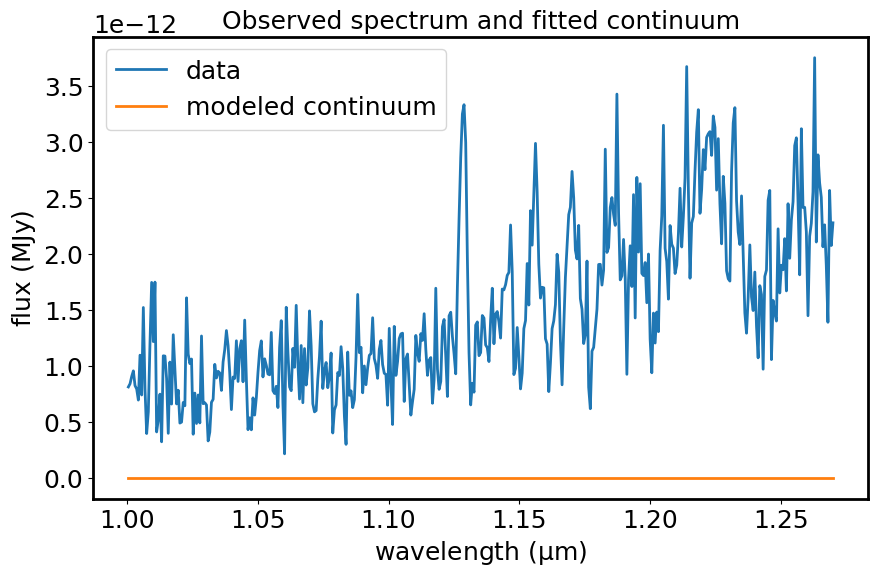
Fit and substract the continuum#
# mask out nans for continuum fitting to work
mask = ~np.isnan(spec1d_masked.flux)
spec1d_masked = Spectrum(spectral_axis = spec1d_masked.spectral_axis[mask],
flux = spec1d_masked.flux[mask], uncertainty = spec1d_masked.uncertainty[mask])
cont_spec1d = fit_generic_continuum(spec1d_masked)
cont_fit = cont_spec1d(spec1d_masked.spectral_axis)
WARNING: Model is linear in parameters; consider using linear fitting methods. [astropy.modeling.fitting]
Developer note: fit_generic_continuum is not fitting right at the moment. Need to investigate.
plt.figure(figsize=[10, 6])
plt.plot(spec1d_masked.spectral_axis, spec1d_masked.flux, label="data")
plt.plot(spec1d_masked.spectral_axis, cont_fit, label="modeled continuum")
plt.xlabel("wavelength ({:latex})".format(spec1d_masked.spectral_axis.unit))
plt.ylabel("flux ({:latex})".format(spec1d_masked.flux.unit))
plt.legend()
plt.title("Observed spectrum and fitted continuum")
plt.show()
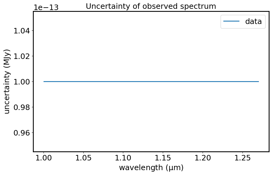
plt.figure(figsize=[10, 6])
plt.plot(spec1d_masked.spectral_axis, spec1d_masked.uncertainty.array, label="data")
plt.xlabel("wavelength ({:latex})".format(spec1d_masked.spectral_axis.unit))
plt.ylabel("uncertainty ({:latex})".format(spec1d_masked.uncertainty.unit))
plt.legend()
plt.title("Uncertainty of observed spectrum")
plt.show()
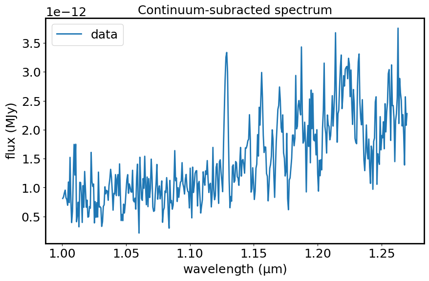
Creating the continuum-subtracted spectrum#
Specutils will figure out what to do with the uncertainty!
spec1d_sub = spec1d_masked - cont_fit
spec1d_sub
<Spectrum(flux=[8.116049726856689e-13 ... 2.2790398562443084e-12] MJy (shape=(425,), mean=0.00000 MJy); spectral_axis=<SpectralAxis
(observer to target:
radial_velocity=0.0 km / s
redshift=0.0)
[1.00061114 1.001246 1.00188086 ... 1.26852317 1.26915803 1.26979289] um> (length=425); uncertainty=StdDevUncertainty)>
plt.figure(figsize=[10, 6])
plt.plot(spec1d_sub.spectral_axis, spec1d_sub.flux, label="data")
plt.xlabel("wavelength ({:latex})".format(spec1d_sub.spectral_axis.unit))
plt.ylabel("flux ({:latex})".format(spec1d_sub.flux.unit))
plt.legend()
plt.title("Continuum-subracted spectrum")
plt.show()
plt.figure(figsize=[10, 6])
plt.plot(spec1d_sub.spectral_axis, spec1d_sub.uncertainty.array, label="data")
plt.xlabel("wavelength ({:latex})".format(spec1d_sub.spectral_axis.unit))
plt.ylabel("uncertainty ({:latex})".format(spec1d_sub.uncertainty.unit))
plt.legend()
plt.title("Uncertainty of continuum-subracted spectrum")
plt.show()
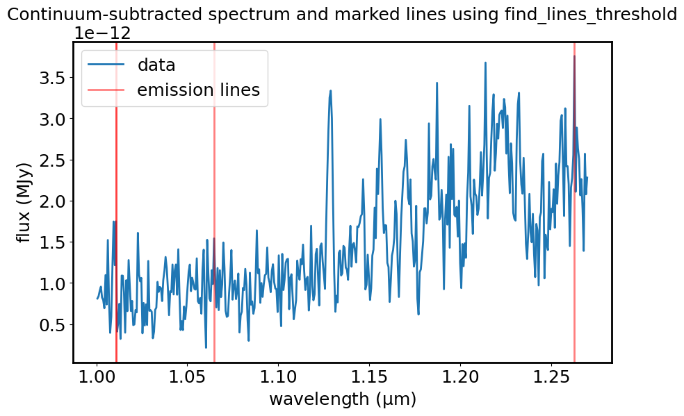
Find emission and absorption lines#
lines = find_lines_threshold(spec1d_sub, noise_factor=3)
lines
WARNING: Spectrum is not below the threshold signal-to-noise 0.01. This may indicate you have not continuum subtracted this spectrum (or that you have but it has high SNR features).
If you want to suppress this warning either type 'specutils.conf.do_continuum_function_check = False' or see http://docs.astropy.org/en/stable/config/#adding-new-configuration-items for other ways to configure the warning. [specutils.analysis.flux]
| line_center | line_type | line_center_index |
|---|---|---|
| um | ||
| float64 | str8 | int64 |
| 1.010768939564626 | emission | 16 |
| 1.0647322627619047 | emission | 101 |
| 1.262809402027211 | emission | 413 |
Plot the emission lines on the spectrum.
plt.figure(figsize=[10, 6])
plt.plot(spec1d_sub.spectral_axis, spec1d_sub.flux, label="data")
plt.axvline(lines['line_center'][0].value, color="red", alpha=0.5, label='emission lines')
for line in lines:
if line['line_type'] == 'emission':
plt.axvline(line['line_center'].value, color='red', alpha=0.5)
plt.xlabel("wavelength ({:latex})".format(spec1d_sub.spectral_axis.unit))
plt.ylabel("flux ({:latex})".format(spec1d_sub.flux.unit))
plt.legend()
plt.title("Continuum-subtracted spectrum and marked lines using find_lines_threshold")
plt.show()
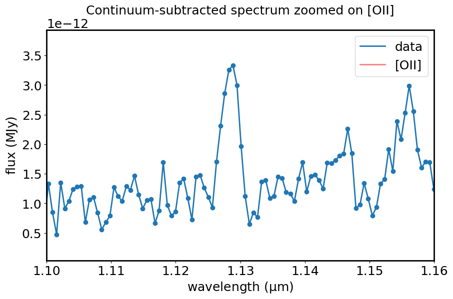
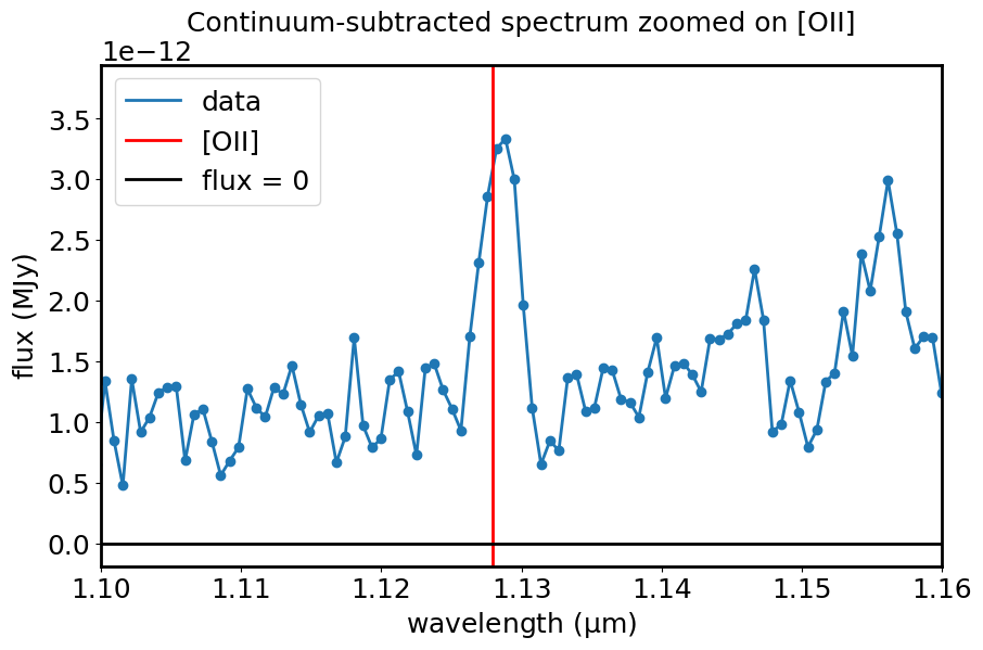
Work by hand on a single line.
# Define limits for plotting
x_min = 1.1
x_max = 1.16
# Define limits for line region
line_min = 1.124*u.um
line_max = 1.131*u.um
plt.figure(figsize=[10, 6])
plt.plot(spec1d_sub.spectral_axis, spec1d_sub.flux, label="data")
plt.scatter(spec1d_sub.spectral_axis, spec1d_sub.flux, label=None)
plt.axvline(lines['line_center'][0].value, color="red", alpha=0.5, label='[OII]')
for line in lines:
if line['line_type'] == 'emission':
plt.axvline(line['line_center'].value, alpha=0.5, color='red')
plt.xlim(x_min, x_max)
plt.xlabel("wavelength ({:latex})".format(spec1d_sub.spectral_axis.unit))
plt.ylabel("flux ({:latex})".format(spec1d_sub.flux.unit))
plt.legend()
plt.title("Continuum-subtracted spectrum zoomed on [OII]")
plt.show()
Measure line centroids and fluxes#
# Example with just one line
centroid(spec1d_sub, SpectralRegion(line_min, line_max))
sline = centroid(spec1d_sub, SpectralRegion(line_min, line_max))
plt.figure(figsize=[10, 6])
plt.plot(spec1d_sub.spectral_axis, spec1d_sub.flux, label="data")
plt.scatter(spec1d_sub.spectral_axis, spec1d_sub.flux, label=None)
plt.axvline(sline.value, color='red', label="[OII]")
plt.axhline(0, color='black', label='flux = 0')
plt.xlim(x_min, x_max)
plt.xlabel("wavelength ({:latex})".format(spec1d_sub.spectral_axis.unit))
plt.ylabel("flux ({:latex})".format(spec1d_sub.flux.unit))
plt.legend()
plt.title("Continuum-subtracted spectrum zoomed on [OII]")
plt.show()
line_flux(spec1d_sub, SpectralRegion(line_min, line_max))
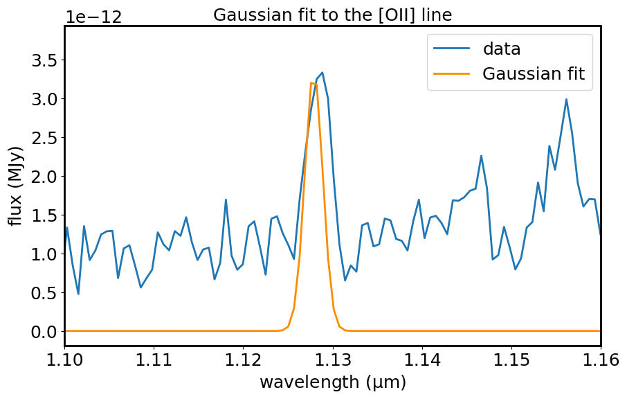
Fit the line with a Gaussian#
g_init = models.Gaussian1D(mean=1.1278909*u.um, stddev=0.001*u.um)
g_fit = fit_lines(spec1d_sub, g_init)
spec1d_fit = g_fit(spec1d_sub.spectral_axis)
g_fit
<Gaussian1D(amplitude=0. MJy, mean=1.1278909 um, stddev=0.001 um)>
plt.figure(figsize=[10, 6])
plt.plot(spec1d_sub.spectral_axis, spec1d_sub.flux, label='data')
plt.plot(spec1d_sub.spectral_axis, spec1d_fit, color='darkorange', label='Gaussian fit')
plt.xlim(x_min, x_max)
plt.xlabel("wavelength ({:latex})".format(spec1d_sub.spectral_axis.unit))
plt.ylabel("flux ({:latex})".format(spec1d_sub.flux.unit))
plt.legend()
plt.title('Gaussian fit to the [OII] line')
plt.show()
Measure the equivalent width of the lines#
This needs the spectrum continuum normalized.
spec1d_norm = spec1d_masked / cont_fit
plt.figure(figsize=[10, 6])
plt.plot(spec1d_norm.spectral_axis, spec1d_norm.flux, label='data')
plt.axhline(1, color='black', label='flux = 1')
plt.xlabel("wavelength ({:latex})".format(spec1d_norm.spectral_axis.unit))
plt.ylabel("flux (normalized)")
plt.xlim(x_min, x_max)
plt.legend()
plt.title("Continuum-normalized spectrum, zoomed on [OII]")
plt.show()
plt.figure(figsize=[10, 6])
plt.plot(spec1d_norm.spectral_axis, spec1d_norm.uncertainty.array, label='data')
plt.xlabel("wavelength ({:latex})".format(spec1d_norm.spectral_axis.unit))
plt.ylabel("uncertainty (normalized)")
plt.xlim(x_min, x_max)
plt.legend()
plt.title("Uncertainty of continuum-normalized spectrum, zoomed on [OII]")
plt.show()
equivalent_width(spec1d_norm, regions=SpectralRegion(line_min, line_max))
Find the best-fitting template#
It needs a list of templates and the redshift of the observed galaxy. For the templates, I am using a set of model SEDs generated with Bruzual & Charlot stellar population models, emission lines, and dust attenuation as described in Pacifici et al. (2012).
Developer note
Maybe there is a way to speed this up (maybe using astropy model_sets)? This fit is run with 100 models, but ideally, if we want to extract physical parameters from this, we would need at least 10,000 models. A dictionary structure with meaningful keys (which can be, e.g., tuples of the relevant physical parameters) could be better than a list? It could make later analysis much clearer than having to map from the list indices back to the relevant parameters.
templatedir = './mos_spectroscopy/templates/'
# Redshift taken from the Specviz analysis
zz = 2.0256
f_lamb_units = u.erg / u.s / (u.cm**2) / u.AA
templatelist = []
# Run on 30 out of 100 for speed
for i in range(1, 30):
template_file = "{0}{1:05d}.dat".format(templatedir, i)
template = ascii.read(template_file)
temp1d = Spectrum(spectral_axis=(template['col1']/1E4)*u.um, flux=template['col2']*f_lamb_units)
templatelist.append(temp1d)
# Change the units of the observed spectrum to match the template
spec1d_masked_flamb = spec1d_masked.with_flux_unit(f_lamb_units)
# The new_flux_unit function does not change the uncertainty and specviz complains that there is a mismatch
# so we re-add the uncertainty like we did a few cells above
spec1d_masked_flamb_unc = Spectrum(spectral_axis=spec1d_masked_flamb.spectral_axis,
flux=spec1d_masked_flamb.flux,
uncertainty=StdDevUncertainty((np.zeros(len(spec1d_masked_flamb.flux)) + 1E-20) * spec1d_masked_flamb.unit))
INFO: the associated NDData object was deleted and cannot be accessed anymore. You can prevent the NDData object from being deleted by assigning it to a variable. If this happened after unpickling make sure you pickle the parent not the uncertainty directly. [astropy.nddata.nduncertainty]
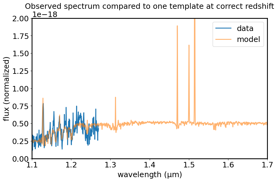
# Take a look at the observed spectrum and one of the templates at the correct redshift
mean_obs = np.mean(spec1d_masked_flamb_unc.flux)
mean_temp = np.mean(templatelist[0].flux)
temp_for_plot = Spectrum(spectral_axis=templatelist[0].spectral_axis * (1.+zz),
flux=templatelist[0].flux*mean_obs/mean_temp)
plt.figure(figsize=[10, 6])
plt.plot(spec1d_masked_flamb_unc.spectral_axis, spec1d_masked_flamb_unc.flux, label='data')
plt.plot(temp_for_plot.spectral_axis, temp_for_plot.flux, label='model', alpha=0.6)
plt.xlabel("wavelength ({:latex})".format(spec1d_masked_flamb_unc.spectral_axis.unit))
plt.ylabel("flux (normalized)")
plt.xlim(1.1, 1.7)
plt.ylim(0, 2e-18)
plt.legend()
plt.title("Observed spectrum compared to one template at correct redshift")
plt.show()
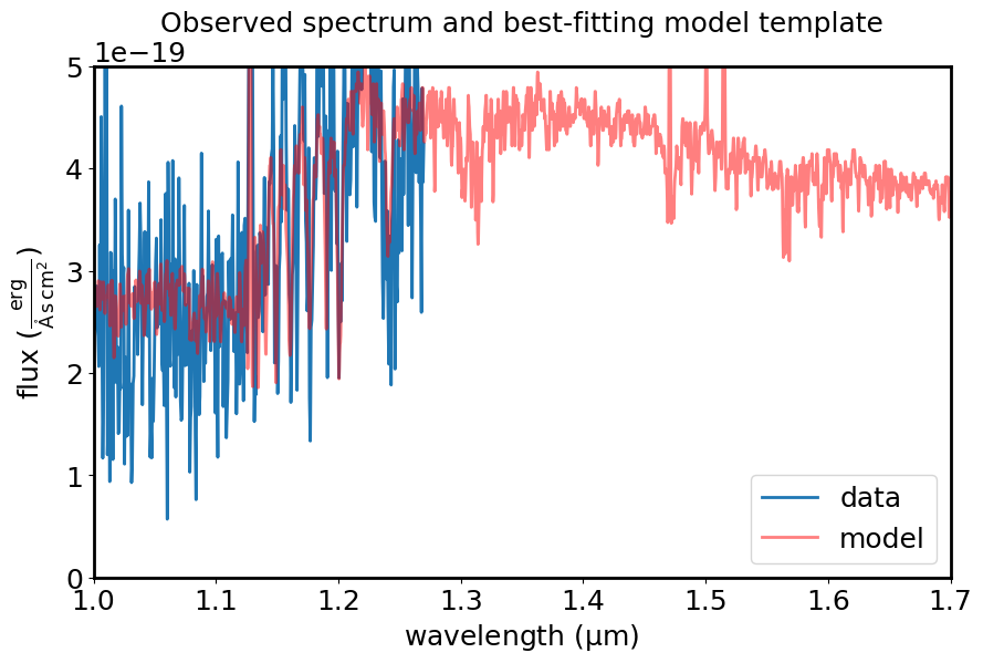
tm_results = template_comparison.template_match(observed_spectrum=spec1d_masked_flamb_unc,
spectral_templates=templatelist,
resample_method="flux_conserving",
redshift=zz)
tm_results[0]
<Spectrum(flux=[0.0 ... 4.828094850492088e-22] erg / (Angstrom s cm2) (shape=(11283,), mean=0.00000 erg / (Angstrom s cm2)); spectral_axis=<SpectralAxis
(observer to target:
radial_velocity=240744.80805001882 km / s
redshift=2.0256)
[ 0.03046779 0.0307401 0.0310124 ... 29.34832 29.469344
29.590368 ] um> (length=11283))>
plt.figure(figsize=[10, 6])
plt.plot(spec1d_masked_flamb_unc.spectral_axis, spec1d_masked_flamb_unc.flux, label="data")
plt.plot(tm_results[0].spectral_axis, tm_results[0].flux, color='r', alpha=0.5, label='model')
plt.xlim(1.0, 1.7)
plt.ylim(0, 5e-19)
plt.xlabel("wavelength ({:latex})".format(spec1d_masked_flamb_unc.spectral_axis.unit))
plt.ylabel("flux ({:latex})".format(spec1d_masked_flamb_unc.flux.unit))
plt.legend()
plt.title("Observed spectrum and best-fitting model template")
plt.show()
New instance of Jdaviz with spectrum and template#
Passing the spectra with different (but compatible) units. Jdaviz adopts the first and converts the second spectrum appropriately.
specviz_2 = jd.new_app()
specviz_2.load(spec1d_masked, format='1D Spectrum', data_label='observed') # This is in MJy
specviz_2.load(tm_results[0], format='1D Spectrum', data_label='model') # This is in erg/(s cm^2 A)
specviz_2.show()

Notebook created by Camilla Pacifici (cpacifici@stsci.edu)
Updated on May 5, 2026