WFSS Spectra Part 0: Optimal Extraction

Use case: optimal extraction of grism spectra; redshift measurement; emission-line maps. Simplified version of JDox Science Use Case # 33.
Data: JWST simulated NIRISS images from MIRAGE, run through the JWST calibration pipeline; galaxy cluster.
Tools: specutils, astropy, pandas, emcee, lmfit, corner, h5py.
Cross-intrument: NIRSpec
Documentation: This notebook is part of a STScI’s larger post-pipeline Data Analysis Tools Ecosystem.

Introduction

This notebook is 1 of 4 in a set focusing on NIRISS WFSS data: 1. 1D optimal extraction since the JWST pipeline only provides a box extraction. Optimal extraction improves S/N of spectra for faint sources. 2. Combine and normalize 1D spectra. 3. Cross correlate galaxy with template to get redshift. 4. Spatially resolved emission line map.

This notebook will start with post-pipeline products of NIRISS WFSS, 2D rectified spectra, from spec level3.

Optimal extraction requires source morphology along the cross-dispersion direction, which will be retrieved from direct images taken along with WFSS observations. Morphology along dispersion direction is also essential to infer the spectral resolution, which will be obtained using template fitting to get redshift and stellar population in notebook #3 of this set.

Note: We here assume reduction of the 2D rectified spectrum has been performed at a decent level, i.e. there is no contaminating flux from other sources on the target 2D spectrum, and that background is already subtracted.

%matplotlib inline

import os
import numpy as np
from scipy.ndimage import rotate
from scipy.optimize import curve_fit

from astropy.io import fits
import astropy.units as u
import astropy.wcs as wcs
from astropy.io import ascii

from specutils import Spectrum1D
from astropy.nddata import StdDevUncertainty

import specutils
print('specutils', specutils.__version__)

import astropy
print('astropy', astropy.__version__)

specutils 1.12.0
astropy 6.0.0

The version should be

• specutils 1.11.0

• astropy 5.3.4

import matplotlib.pyplot as plt
import matplotlib as mpl

mpl.rcParams['savefig.dpi'] = 80
mpl.rcParams['figure.dpi'] = 80

0.Download and load data:

These include pipeline processed data for NIRISS, as well as photometric catalog from image step3.

if not os.path.exists('./pipeline_products'):
    import zipfile
    import urllib.request
    boxlink = 'https://data.science.stsci.edu/redirect/JWST/jwst-data_analysis_tools/NIRISS_lensing_cluster/pipeline_products.zip'
    boxfile = './pipeline_products.zip'
    urllib.request.urlretrieve(boxlink, boxfile)
    zf = zipfile.ZipFile(boxfile, 'r')
    zf.extractall()

DIR_DATA = './pipeline_products/'

# Output directory;
DIR_OUT = './output/'
if not os.path.exists(DIR_OUT):
    os.mkdir(DIR_OUT)

# Filter for detection and science image;
filt_det = 'f200w'

# Image array from direct image. This is for optimal extraction and masking.
# This image should already be sky-subtracted; otherwise, you will encounter a wrong result with optimal extraction.

infile = f'{DIR_DATA}l3_nis_{filt_det}_i2d_skysub.fits'
hdu = fits.open(infile)

# This is just for error array;
infile = f'{DIR_DATA}l3_nis_{filt_det}_i2d.fits'
hdu_err = fits.open(infile)

data = hdu[0].data
imwcs = wcs.WCS(hdu[0].header, hdu)

err = hdu_err[2].data
weight = 1/np.square(err)

# Segmentation map;
# This can be prepared by running Photutils, if the pipeline does not generate one.
segfile = f'{DIR_DATA}l3_nis_{filt_det}_i2d_seg.fits'
seghdu = fits.open(segfile)
segdata = seghdu[0].data

/tmp/ipykernel_2017/874489203.py:25: RuntimeWarning: divide by zero encountered in divide
  weight = 1/np.square(err)

# Load catalog from image level3;
# to obtain source position in pixel coordinate.
catfile = f'{DIR_DATA}l3_nis_{filt_det}_cat.ecsv'
fd = ascii.read(catfile)

fd

QTable length=7

id	xcentroid	ycentroid	sky_centroid	aper_bkg_flux	aper_bkg_flux_err	aper30_flux	aper30_flux_err	aper50_flux	aper50_flux_err	aper70_flux	aper70_flux_err	aper_total_flux	aper_total_flux_err	aper30_abmag	aper30_abmag_err	aper50_abmag	aper50_abmag_err	aper70_abmag	aper70_abmag_err	aper_total_abmag	aper_total_abmag_err	aper30_vegamag	aper30_vegamag_err	aper50_vegamag	aper50_vegamag_err	aper70_vegamag	aper70_vegamag_err	aper_total_vegamag	aper_total_vegamag_err	CI_30_50	CI_50_70	CI_30_70	is_star	sharpness	roundness	nn_dist	nn_abmag	isophotal_flux	isophotal_flux_err	isophotal_abmag	isophotal_abmag_err	isophotal_vegamag	isophotal_vegamag_err	isophotal_area	semimajor_sigma	semiminor_sigma	ellipticity	orientation	sky_orientation	sky_bbox_ll	sky_bbox_ul	sky_bbox_lr	sky_bbox_ur
	pix	pix	deg,deg	Jy	Jy	Jy	Jy	Jy	Jy	Jy	Jy	Jy	Jy																							pix		Jy	Jy					pix2	pix	pix		deg	deg	deg,deg	deg,deg	deg,deg	deg,deg
int64	float64	float64	SkyCoord	float64	float64	float64	float64	float64	float64	float64	float64	float64	float64	float64	float64	float64	float64	float64	float64	float64	float64	float64	float64	float64	float64	float64	float64	float64	float64	float64	float64	float64	float64	float64	float32	float64	float64	float64	float32	float64	float64	float64	float64	float64	float64	float64	float64	float64	float64	SkyCoord	SkyCoord	SkyCoord	SkyCoord
1	1901.4791	616.6617	3.569653944921018,-30.405070186723776	3.483045e-08	nan	8.130363e-08	nan	1.921404e-07	nan	3.765590e-07	nan	nan	nan	26.624725	nan	25.690953	nan	24.960418	nan	nan	nan	24.915445	nan	23.981673	nan	23.251138	nan	nan	nan	0.9338	0.7305	1.6643	nan	0.643053	0.050833	687.142856	22.245099	3.217875e-06	nan	22.631077	nan	20.921797	nan	83.0	2.300009	2.249340	0.022030	-68.272405	22.344833	3.569758007135362,-30.405165289935546	3.5697605503538763,-30.404964734861768	3.56952547091111,-30.405163096272904	3.5695280146070885,-30.404962541203844
2	1215.5473	657.4411	3.5841636319830568,-30.40446267443482	4.591611e-08	nan	1.550019e-07	nan	3.638838e-07	nan	6.725310e-07	nan	nan	nan	25.924158	nan	24.997593	nan	24.330719	nan	nan	nan	24.214878	nan	23.288313	nan	22.621439	nan	nan	nan	0.9266	0.6669	1.5934	nan	0.666481	0.076069	687.142856	22.631077	4.591563e-06	nan	22.245099	nan	20.535819	nan	95.0	2.968964	1.778262	0.401050	89.747234	180.364471	3.5842476045730627,-30.404590023798825	3.5842510319996697,-30.404316539215852	3.5840573485032308,-30.404588250016765	3.58406077646256,-30.404314765438812
3	381.9250	984.5165	3.601859711428753,-30.398662437780448	4.268341e-08	nan	1.404209e-07	nan	3.172360e-07	nan	6.277053e-07	nan	nan	nan	26.031420	nan	25.146544	nan	24.405610	nan	nan	nan	24.322140	nan	23.437264	nan	22.696330	nan	nan	nan	0.8849	0.7409	1.6258	nan	0.672185	0.331872	673.406986	16.320658	4.647145e-06	nan	22.232034	nan	20.522754	nan	101.0	2.880019	1.989674	0.309146	-89.237463	1.379775	3.6019516675347565,-30.39879122365138	3.601955045183127,-30.39851773861101	3.6017402841066257,-30.398789281273874	3.60174366234683,-30.398515796238758
4	1100.5677	1408.4408	3.5867654957418873,-30.390792851961756	4.182255e-08	nan	1.977441e-07	nan	4.634087e-07	nan	8.557904e-07	nan	nan	nan	25.659741	nan	24.735090	nan	24.069081	nan	nan	nan	23.950461	nan	23.025810	nan	22.359801	nan	nan	nan	0.9247	0.6660	1.5907	nan	0.675891	0.239616	759.750606	22.245099	4.479109e-06	nan	22.272021	nan	20.562741	nan	78.0	2.864331	1.524197	0.467870	89.968483	180.585720	3.586849890460872,-30.390920199626773	3.586853310121526,-30.390646714975425	3.586659660970119,-30.390918429617493	3.586663081163341,-30.39064494497111
5	662.4288	1685.1702	3.596088874688556,-30.385833272645225	3.108490e-08	nan	6.850841e-07	nan	1.445057e-06	nan	2.486505e-06	nan	nan	nan	24.310640	nan	23.500287	nan	22.911026	nan	nan	nan	22.601360	nan	21.791007	nan	21.201746	nan	nan	nan	0.8104	0.5893	1.3996	nan	0.584634	-0.067064	334.076772	20.727265	5.441945e-06	nan	22.060615	nan	20.351335	nan	71.0	1.874113	1.820229	0.028752	10.431093	101.048330	3.5961919899951726,-30.38591938323127	3.5961942522168715,-30.385737059975185	3.5959594989853887,-30.38591723639035	3.5959617616410102,-30.38573491313818
6	319.4990	1885.3035	3.60338188710553,-30.382251101963146	3.326749e-08	nan	6.893335e-07	nan	1.514847e-06	nan	2.523116e-06	nan	nan	nan	24.303927	nan	23.449078	nan	22.895157	nan	nan	nan	22.594647	nan	21.739798	nan	21.185877	nan	nan	nan	0.8548	0.5539	1.4088	nan	0.581781	0.158721	111.504109	22.028328	5.666923e-06	nan	22.016632	nan	20.307352	nan	75.0	1.894424	1.866322	0.014834	14.267744	104.884981	3.603486459620283,-30.38233965159385	3.603488932995949,-30.382139095884135	3.6032539769794103,-30.38233751766547	3.6032564508323546,-30.382136961959965
7	266.9182	1983.6317	3.604515260247416,-30.380468545121307	3.310798e-08	nan	7.155692e-07	nan	1.476385e-06	nan	2.520043e-06	nan	nan	nan	24.263371	nan	23.477001	nan	22.896480	nan	nan	nan	22.554091	nan	21.767721	nan	21.187200	nan	nan	nan	0.7864	0.5805	1.3669	nan	0.593763	0.061278	111.504109	22.016632	5.606203e-06	nan	22.028328	nan	20.319048	nan	74.0	1.893807	1.847921	0.024230	89.641888	180.259126	3.6046074836711655,-30.380562964468123	3.6046099547002646,-30.380362408741654	3.6043961396388418,-30.38056102635311	3.6043986111017956,-30.38036047063047

Make a broadband flux catalog.

• For a convenient reason, here we compile catalogs into a flux catalog, which will be used in the following notebook (01b).

• To run this cell, you will need a photometric catalog of sources, that list sources position and flux for each filter. For now, I use this catalog prepared in another notebook. (“sources_extend_01.cat”)

• This catalog can also be used for generic phot-z/SED fitting softwares, like EAZY and gsf (see notebook No.04).

For now, we use an input catalog.

filts = ['f115w', 'f150w', 'f200w', 'f090w', 'f435w', 'f606w', 'f814w', 'f105w', 'f125w', 'f140w', 'f160w']
eazy_filts = [309, 310, 311, 308, 1, 4, 6, 202, 203, 204, 205]
magzp = 25.0 # magnitude zeropoint in the catalog.

# Read catalog;
fd_input = ascii.read(f'{DIR_DATA}sources_extend_01.cat')
ra_input = fd_input['x_or_RA']
dec_input = fd_input['y_or_Dec']

# Header;
fw = open(f'{DIR_OUT}l3_nis_flux.cat', 'w')
fw.write('# id')
for ff in range(len(filts)):
    fw.write(f' F{eazy_filts[ff]} E{eazy_filts[ff]}')
fw.write('\n')

# Contents;
for ii in range(len(fd['id'])):
    
    rtmp = np.sqrt((fd['sky_centroid'].ra.value[ii] - ra_input[:])**2 + (fd['sky_centroid'].dec.value[ii] - dec_input[:])**2)
    iix = np.argmin(rtmp)
    
    for ff in range(len(filts)):
        if ff == 0:
            fw.write(f"{fd['id'][ii]}")

        mag = fd_input[f'niriss_{filts[ff]}_magnitude'][iix]
        flux_nu = 10**((mag-magzp)/(-2.5))

        # Currently, the catalog does not provide proper error;
        # Assuming a 5% error for flux.
        
        flux_err_nu = flux_nu * 0.05

        fw.write(f' {flux_nu:.5e} {flux_err_nu:.5e}') 

    fw.write('\n')
fw.close()

1.Load 2D spectrum;

# Which filter, grating, and object?
filt = 'f200w'

# grism = 'G150R'
grism = 'G150C'

id = '00004'

# Zero-indexed number for dither --- the test data here has two dither positions, so 0 or 1.
ndither = 0

file_2d = f'{DIR_DATA}l3_nis_{filt}_{grism}_s{id}_cal.fits'
hdu_2d = fits.open(file_2d)

# Align grism direction
#   - x-direction = Dispersion (wavelength) direction.
#   - y-direction = Cross-dispersion.
# in this notebook.
    
if grism == 'G150C':
    # If spectrum is horizontal;
    data_2d = hdu_2d[ndither*7+1].data
    dq_2d = hdu_2d[ndither*7+2].data
    err_2d = hdu_2d[ndither*7+3].data
    wave_2d = hdu_2d[ndither*7+4].data
else:
    data_2d = rotate(hdu_2d[ndither*7+1].data, 90)
    dq_2d = rotate(hdu_2d[ndither*7+2].data, 90)
    err_2d = rotate(hdu_2d[ndither*7+3].data, 90)
    wave_2d = rotate(hdu_2d[ndither*7+4].data, 90)

# Get position angle of observation;
hd_2d = hdu_2d[1].header
PA_V3 = hd_2d['PA_V3']
PA_V3

0.0

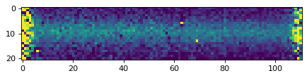
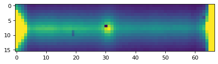
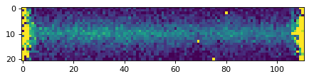
plt.imshow(data_2d, vmin=0, vmax=1000)

<matplotlib.image.AxesImage at 0x7fa114afba90>

# Get light profile of the source;

# Again, y is for cross-dispersion, and x is for dispersion directions.
y2d, x2d = data_2d.shape[:]

# Cut out segmentation map;
iix = np.where(fd['id'] == int(id))[0][0]

# Target position from image 3 catalog;
ycen = fd['ycentroid'][iix].value
xcen = fd['xcentroid'][iix].value

# Cutout size = y direction of 2D spectrum;
rsq = y2d

sci_cut = data[int(ycen-rsq/2.+0.5):int(ycen+rsq/2.+0.5), int(xcen-rsq/2.+0.5):int(xcen+rsq/2.+0.5)]
seg_cut = segdata[int(ycen-rsq/2.+0.5):int(ycen+rsq/2.+0.5), int(xcen-rsq/2.+0.5):int(xcen+rsq/2.+0.5)]

# Rotate image for PA of Grism observation;
if grism == 'G150C':
    sci_rot = rotate(sci_cut, PA_V3)
else:
    sci_rot = rotate(sci_cut, PA_V3+90)

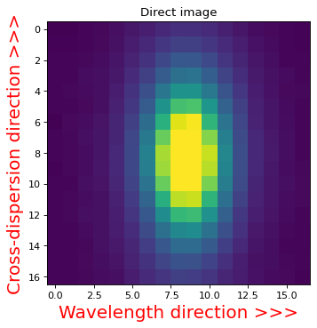
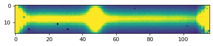
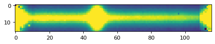
WFSS grism is dispersed in a direction of x-axis in the plot below.

plt.imshow(sci_rot, vmin=0, vmax=1.0)
plt.title('Direct image')
plt.xlabel('Wavelength direction >>>', color='r', fontsize=18)
plt.ylabel('Cross-dispersion direction >>>', color='r', fontsize=18)

Text(0, 0.5, 'Cross-dispersion direction >>>')

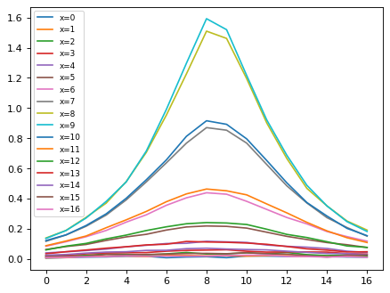
2.Get light profile at different x position — This will be used for optimal extraction.

for ii in range(sci_rot.shape[1]):
    flux_tmp = sci_rot[:, ii]
    xx_tmp = np.arange(0, len(sci_rot[:, ii]), 1)
    plt.plot(xx_tmp, flux_tmp, label='x={}'.format(ii))
plt.legend(loc=0, fontsize=8)

<matplotlib.legend.Legend at 0x7fa114a4c3d0>

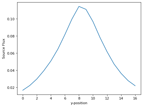
# Sum along x (disperse) direction
flux_y = np.zeros(len(sci_rot[:, 0]), 'float')
for ii in range(sci_rot.shape[0]):
    flux_y[ii] = np.sum(sci_rot[ii, :])

# Sky subtraction, if needed.
# sky = np.mean([flux_y[0], flux_y[-1]])

# Normalize;
flux_y[:] /= flux_y.sum()

plt.plot(xx_tmp, flux_y)
plt.xlabel('y-position')
plt.ylabel('Source Flux')

Text(0, 0.5, 'Source Flux')

3.One-dimensional extraction;

Show pipeline 1D extraction as an example;

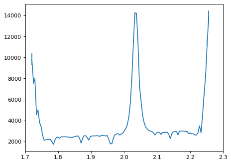
# Normal extraction;
flux_disp1 = np.zeros(x2d, 'float')
err_disp1 = np.zeros(x2d, 'float')
wave_disp1 = np.zeros(x2d, 'float')
    
for ii in range(x2d): # Wavelength direction.
    mask_tmp = (dq_2d[:, ii] == 0) & (err_2d[:, ii] > 0)

    # Sum within a box;
    flux_disp1[ii] = np.sum(data_2d[:, ii][mask_tmp]) 
    err_disp1[ii] = np.sqrt(np.sum(err_2d[:, ii][mask_tmp]**2)) 
    wave_disp1[ii] = wave_2d[0, ii]

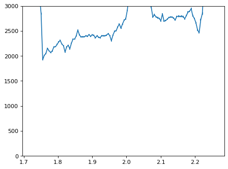
plt.errorbar(wave_disp1, flux_disp1, yerr=err_disp1)
plt.xlim(1.7, 2.3)

(1.7, 2.3)

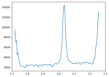
Optimal extraction;

# Following Horne(1986, PASP, 98, 609);
flux_disp = np.zeros(x2d, 'float')
err_disp = np.zeros(x2d, 'float')
wave_disp = np.zeros(x2d, 'float')

# Sigma clipping.
sig = 5.0

for ii in range(x2d): # ii : wavelength element.
    # Mask; 
    # 1. DQ array
    # 2. error value
    # 3. CR detection
    mask_tmp = (dq_2d[:, ii] == 0) & (err_2d[:, ii] > 0) & ((data_2d[:, ii] - flux_y[:] * flux_disp1[ii])**2 < sig**2 * err_2d[:, ii]**2)
    ivar = 1. / err_2d[:, ii]**2

    num = flux_y[:] * data_2d[:, ii] * ivar
    den = flux_y[:]**2 * ivar
    flux_disp[ii] = num[mask_tmp].sum(axis=0) / den[mask_tmp].sum(axis=0)
    err_disp[ii] = np.sqrt(1./den[mask_tmp].sum(axis=0))
    wave_disp[ii] = wave_2d[0, ii]
    
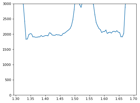
plt.errorbar(wave_disp, flux_disp, yerr=err_disp)
plt.xlim(1.7, 2.3)

(1.7, 2.3)

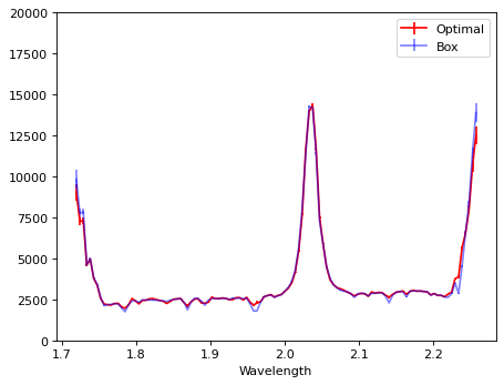
# Compare;
plt.errorbar(wave_disp, flux_disp, yerr=err_disp, color='r', label='Optimal')
plt.errorbar(wave_disp1, flux_disp1, yerr=err_disp1, color='b', alpha=0.5, label='Box')
plt.ylim(-10, 20000)
plt.legend(loc=0)
plt.xlabel('Wavelength')

Text(0.5, 0, 'Wavelength')

4.Write 1d spectrum out to a file;

file_1d = f'{DIR_OUT}l3_nis_{filt}_{grism}_s{id}_1d_opt.fits'

# Now make it into a Spectrum1D instance.
obs = Spectrum1D(spectral_axis=wave_disp*u.um,
                 flux=flux_disp*u.MJy,
                 uncertainty=StdDevUncertainty(err_disp), unit='MJy')
obs.write(file_1d, format='tabular-fits', overwrite=True)

5.Light profile along x-axis = Resolution of dispersed spectrum;

As WFSS does not have a slit, any dispersed spectrum is affected by source morphology. The estimate on the effective spectral resolution will be needed in the following notebook. And we here try to estimate it beforehand;

for ii in range(sci_rot.shape[0]):
    flux_tmp = sci_rot[ii, :]
    xx_tmp = np.arange(0, len(sci_rot[ii, :]), 1)
    plt.plot(xx_tmp, flux_tmp, label=f'y={ii}')
    
plt.legend(loc=1, fontsize=8)
plt.xlabel('Wavelength direction')
plt.title('Source light profile along dispersed direction', fontsize=14)

Text(0.5, 1.0, 'Source light profile along dispersed direction')

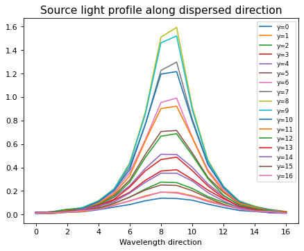
*Unless you are interested in spatially resolved spectra, you can stack and get light profile as a good approximation.

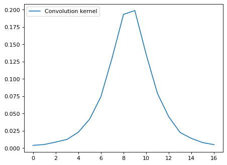
# Sum along cross-disperse direction
flux_x = np.zeros(len(sci_rot[0, :]), 'float')
for ii in range(sci_rot.shape[0]):
    flux_x[ii] = np.sum(sci_rot[:, ii])

# Normalize;
flux_x[:] /= flux_x.sum()

plt.plot(xx_tmp, flux_x, label='Convolution kernel')
plt.legend(loc=2)

<matplotlib.legend.Legend at 0x7fa10f2b3910>

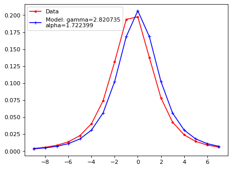
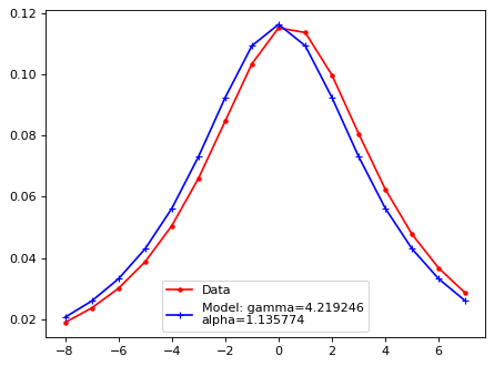
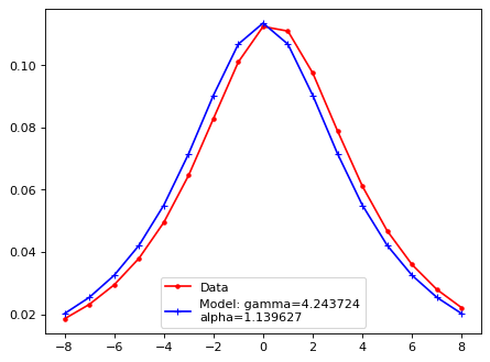
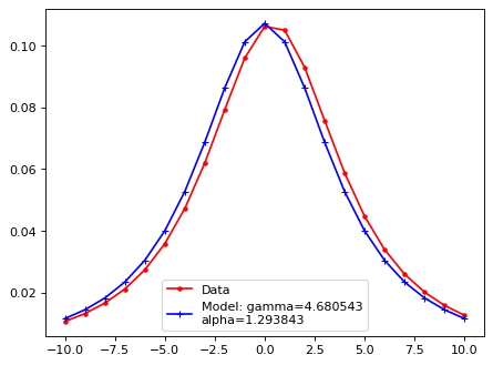
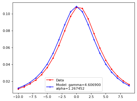
Fit with a moffat function;

# Fitting function with Moffat
# Moffat fnc.

def moffat(xx, A, x0, gamma, alp):
    yy = A * (1. + (xx-x0)**2/gamma**2)**(-alp)
    return yy


def fit_mof(xx, lsf):
    # xx = lsf * 0
    # for ii in range(len(lsf)):
    #    xx[ii] = ii - len(lsf)/2.
    popt, pcov = curve_fit(moffat, xx, lsf)
    return popt


def LSF_mof(xsf, lsf, f_plot=True):
    '''
    Input:
    =======
    xsf : x axis for the profile.
    lsf : light profile.    
    '''
    
    # for ii in range(len(sci[0, :])):
    #    lsf[ii] = np.mean(sci_rot[int(height/2.-5):int(height/2.+5), ii])
    #    xsf[ii] = ii - len(lsf)/2.

    try:
        A, xm, gamma, alpha = fit_mof(xsf, lsf)
    except RuntimeError:
        print('Fitting failed.')
        A, xm, gamma, alpha = -1, -1, -1, -1
        pass

    if A > 0:
        lsf_mod = moffat(xsf, A, 0, gamma, alpha)
        
    if f_plot:
        yy = moffat(xsf, A, xm, gamma, alpha)
        plt.plot(xsf, yy, 'r.', ls='-', label='Data')
        plt.plot(xsf, lsf_mod, 'b+', ls='-', label=f'Model: gamma={gamma:2f}\nalpha={alpha:2f}')
        plt.legend()
        plt.show()
    
    return A, xm, gamma, alpha

# LSF, line spread function
iix_peak = np.argmax(flux_x)
xx_tmp_shift = xx_tmp - xx_tmp[iix_peak]
A, xm, gamma, alpha = LSF_mof(xx_tmp_shift, flux_x)

# Write it down;
# Tha parameters are in unit of pixel.
fm = open(f'{DIR_OUT}l3_nis_{filt}_{grism}_s{id}_moffat.txt', 'w')
fm.write('# A x0 gamma alp\n')
fm.write('# Moffat function\n')
fm.write(f'{A:.3f} {xm:.3f} {gamma:.3f} {alpha:.3f}\n')

fm.close()

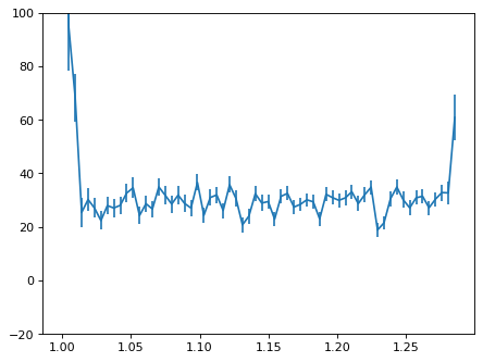
Repeat for other filters, other objects.

The following big colum executes the same processes above for other filters and dither position.

grism = 'G150C'
id = '00004'
DIR_OUT = './output/'
if not os.path.exists(DIR_OUT):
    os.mkdir(DIR_OUT)

filts = ['f115w', 'f150w', 'f200w']
ndithers = np.arange(0, 2, 1)

sig = 5.0

for filt in filts:
    print(filt)
    
    # 2d spectrum;
    file_2d = f'{DIR_DATA}l3_nis_{filt}_{grism}_s{id}_cal.fits'
    hdu_2d = fits.open(file_2d)

    for ndither in ndithers:
        print(ndither)

        if grism == 'G150C':
            # If spectrum is horizontal;
            data_2d = hdu_2d[ndither*7+1].data
            dq_2d = hdu_2d[ndither*7+2].data
            err_2d = hdu_2d[ndither*7+3].data
            wave_2d = hdu_2d[ndither*7+4].data
        else:
            data_2d = rotate(hdu_2d[ndither*7+1].data, 90)
            dq_2d = rotate(hdu_2d[ndither*7+2].data, 90)
            err_2d = rotate(hdu_2d[ndither*7+3].data, 90)
            wave_2d = rotate(hdu_2d[ndither*7+4].data, 90)

        y2d, x2d = data_2d.shape[:]

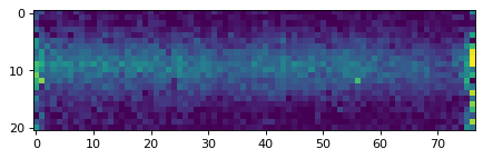
        plt.close()
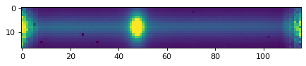
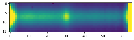
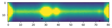
        plt.imshow(data_2d, vmin=0, vmax=300)
        plt.show()

        # Re-extract 2d image;
        # if ndither == 0:
        rsq = y2d
        sci_cut = data[int(ycen-rsq/2.+0.5):int(ycen+rsq/2.+0.5), int(xcen-rsq/2.+0.5):int(xcen+rsq/2.+0.5)]
        seg_cut = segdata[int(ycen-rsq/2.+0.5):int(ycen+rsq/2.+0.5), int(xcen-rsq/2.+0.5):int(xcen+rsq/2.+0.5)]

        # Not sure if the offset in extractioin box is bug ;
        if grism == 'G150C':
            sci_rot = rotate(sci_cut, PA_V3+0)
        else:
            sci_rot = rotate(sci_cut, PA_V3+0+90)

        # This is for spectral resolution;
        # Get light profile along the x-axis
        for ii in range(sci_rot.shape[0]):
            flux_tmp = sci_rot[ii, :]
            xx_tmp = np.arange(0, len(sci_rot[ii, :]), 1)

        # Sum along cross-disperse direction
        flux_x = np.zeros(len(sci_rot[0, :]), 'float')
        for ii in range(sci_rot.shape[0]):
            flux_x[ii] = np.sum(sci_rot[ii, :])

        # Normalize;
        flux_x[:] /= flux_x.sum()

        # LSF
        iix_peak = np.argmax(flux_x)
        xx_tmp_shift = xx_tmp - xx_tmp[iix_peak]
        A, xm, gamma, alpha = LSF_mof(xx_tmp_shift, flux_x)

        if ndither == 0:
            # Write it down;
            fm = open(f'{DIR_OUT}l3_nis_{filt}_{grism}_s{id}_moffat.txt', 'w')
            fm.write('# A x0 gamma alp\n')
            fm.write('# Moffat function\n')
            fm.write(f'{A:.3f} {xm:.3f} {gamma:.3f} {alpha:.3f}\n')
            fm.close()

        # This is for Optimal extraction;
        # Sum along x (disperse) direction
        flux_y = np.zeros(len(sci_rot[:, 0]), 'float')
        for ii in range(sci_rot.shape[0]):
            flux_y[ii] = np.sum(sci_rot[ii, :])
            
        # Normalize;
        flux_y[:] /= flux_y.sum()

        # Following Horne;
        flux_disp = np.zeros(x2d, 'float')
        err_disp = np.zeros(x2d, 'float')
        wave_disp = np.zeros(x2d, 'float')

        for ii in range(x2d):
            # Mask; 
            # 1. DQ array
            # 2. error value
            # 3. CR detection
            mask_tmp = (dq_2d[:, ii] == 0) & (err_2d[:, ii] > 0)
            ivar = 1. / err_2d[:, ii]**2

            num = flux_y[:] * data_2d[:, ii] * ivar 
            den = flux_y[:]**2 * ivar
            flux_disp[ii] = num[mask_tmp].sum(axis=0)/den[mask_tmp].sum(axis=0)
            err_disp[ii] = np.sqrt(1./den[mask_tmp].sum(axis=0))
            wave_disp[ii] = wave_2d[0, ii]

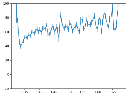
        plt.close()
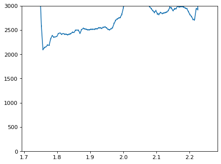
        con_plot = (wave_disp > 0)
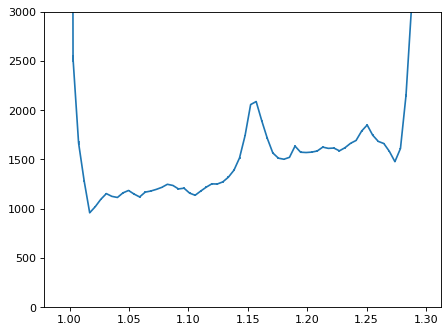
        plt.errorbar(wave_disp[con_plot], flux_disp[con_plot], yerr=err_disp[con_plot])
        plt.ylim(-0, 3000)
        plt.show()

        # Wirte:
        # Now make it into a Spectrum1D instance.
        file_1d = f'{DIR_OUT}l3_nis_{filt}_{grism}_s{id}_ndither{ndither}_1d_opt.fits'

        if wave_disp[1] - wave_disp[0] < 0:
            obs = Spectrum1D(spectral_axis=wave_disp[::-1]*u.um,
                             flux=flux_disp[::-1]*u.MJy,
                             uncertainty=StdDevUncertainty(err_disp[::-1]), unit='MJy')
        else:
            obs = Spectrum1D(spectral_axis=wave_disp*u.um,
                             flux=flux_disp*u.MJy,
                             uncertainty=StdDevUncertainty(err_disp), unit='MJy')
            
        obs.write(file_1d, format='tabular-fits', overwrite=True)

f115w
0

1

f150w
0

1

f200w
0

1

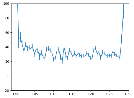
Another object;

Absorption line galaxy

grism = 'G150C'
id = '00003'
DIR_OUT = './output/'

filts = ['f115w', 'f150w', 'f200w']
ndithers = np.arange(0, 2, 1) # There are four dithers in the data set;

sig = 5.0

for filt in filts:
    print(filt)
    # 2d spectrum;
    file_2d = f'{DIR_DATA}l3_nis_{filt}_{grism}_s{id}_cal.fits'
    hdu_2d = fits.open(file_2d)

    for ndither in ndithers:
        print(ndither)
        if grism == 'G150C':
            # If spectrum is horizontal;
            data_2d = hdu_2d[ndither*7+1].data
            dq_2d = hdu_2d[ndither*7+2].data
            err_2d = hdu_2d[ndither*7+3].data
            wave_2d = hdu_2d[ndither*7+4].data
        else:
            data_2d = rotate(hdu_2d[ndither*7+1].data, 90)
            dq_2d = rotate(hdu_2d[ndither*7+2].data, 90)
            err_2d = rotate(hdu_2d[ndither*7+3].data, 90)
            wave_2d = rotate(hdu_2d[ndither*7+4].data, 90)

        y2d, x2d = data_2d.shape[:]

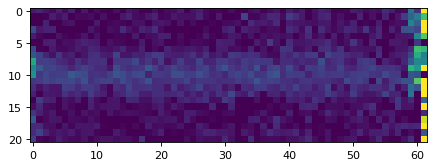
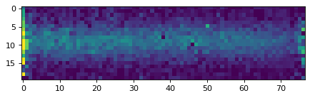
        plt.close()
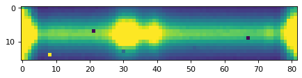
        plt.imshow(data_2d, vmin=0, vmax=20)
        plt.show()

        # Re-extract 2d image;
        # if ndither == 0:
        rsq = y2d
        sci_cut = data[int(ycen-rsq/2.+0.5):int(ycen+rsq/2.+0.5), int(xcen-rsq/2.+0.5):int(xcen+rsq/2.+0.5)]
        seg_cut = segdata[int(ycen-rsq/2.+0.5):int(ycen+rsq/2.+0.5), int(xcen-rsq/2.+0.5):int(xcen+rsq/2.+0.5)]

        # Not sure if the offset in extraction box is bug ;
        if grism == 'G150C':
            sci_rot = rotate(sci_cut, PA_V3+0)
        else:
            sci_rot = rotate(sci_cut, PA_V3+0+90)

        # This is for spectral resolution;
        # Get light profile along the x-axis
        for ii in range(sci_rot.shape[0]):
            flux_tmp = sci_rot[ii, :]
            xx_tmp = np.arange(0, len(sci_rot[ii, :]), 1)

        # Sum along cross-disperse direction
        flux_x = np.zeros(len(sci_rot[0, :]), 'float')
        for ii in range(sci_rot.shape[0]):
            flux_x[ii] = np.sum(sci_rot[ii, :])

        # Normalize;
        flux_x[:] /= flux_x.sum()

        # LSF
        iix_peak = np.argmax(flux_x)
        xx_tmp_shift = xx_tmp - xx_tmp[iix_peak]
        A, xm, gamma, alpha = LSF_mof(xx_tmp_shift, flux_x)

        if ndither == 0:
            # Write it down;
            fm = open(f'{DIR_OUT}l3_nis_{filt}_{grism}_s{id}_moffat.txt', 'w')
            fm.write('# A x0 gamma alp\n')
            fm.write('# Moffat function\n')
            fm.write(f'{A:.3f} {xm:.3f} {gamma:.3f} {alpha:.3f}\n')
            fm.close()

        # This is for Optimal extraction;
        # Sum along x (disperse) direction
        flux_y = np.zeros(len(sci_rot[:, 0]), 'float')
        for ii in range(sci_rot.shape[0]):
            flux_y[ii] = np.sum(sci_rot[ii, :])
    
        # Normalize;
        flux_y[:] /= flux_y.sum()

        # Following Horne;
        flux_disp = np.zeros(x2d, 'float')
        err_disp = np.zeros(x2d, 'float')
        wave_disp = np.zeros(x2d, 'float')

        for ii in range(x2d):
            # Mask; 
            # 1. DQ array
            # 2. error value
            # 3. CR detection
            mask_tmp = (dq_2d[:, ii] == 0) & (err_2d[:, ii] > 0) 
            ivar = 1. / err_2d[:, ii]**2

            num = flux_y[:] * data_2d[:, ii] * ivar 
            den = flux_y[:]**2 * ivar
            flux_disp[ii] = num[mask_tmp].sum(axis=0)/den[mask_tmp].sum(axis=0)
            err_disp[ii] = np.sqrt(1./den[mask_tmp].sum(axis=0))
            wave_disp[ii] = wave_2d[0, ii]

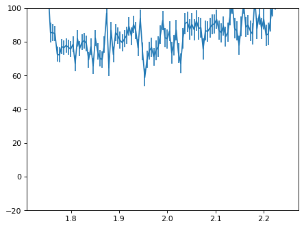
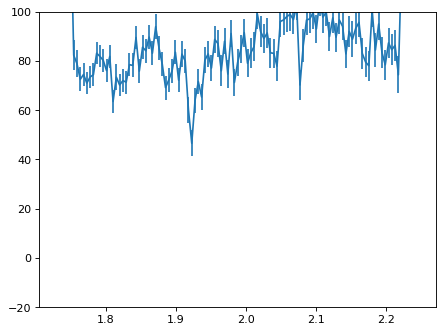
        plt.close()
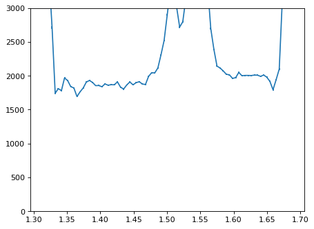
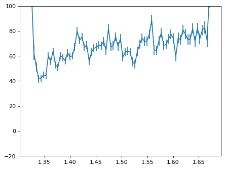
        con_plot = (wave_disp > 0)
        plt.errorbar(wave_disp[con_plot], flux_disp[con_plot], yerr=err_disp[con_plot])
        plt.ylim(-20, 100)
        plt.show()

        # Write:
        # Now, make it into a Spectrum1D instance.
        file_1d = f'{DIR_OUT}l3_nis_{filt}_{grism}_s{id}_ndither{ndither}_1d_opt.fits'

        if wave_disp[1] - wave_disp[0] < 0:
            obs = Spectrum1D(spectral_axis=wave_disp[::-1]*u.um,
                             flux=flux_disp[::-1]*u.MJy,
                             uncertainty=StdDevUncertainty(err_disp[::-1]), unit='MJy')
        else:
            obs = Spectrum1D(spectral_axis=wave_disp*u.um,
                             flux=flux_disp*u.MJy,
                             uncertainty=StdDevUncertainty(err_disp), unit='MJy')

        obs.write(file_1d, format='tabular-fits', overwrite=True)    

f115w
0

1

f150w
0

1

f200w
0

1