NIRCam Wisp Removal#
Author: Ben Sunnquist (bsunnquist@stsci.edu)
Latest Update: 24 July 2024
Use case: NIRCam Imaging detectors A3, A4, B3, and B4.
Data: PID 1063 Obs 6 Imaging Flats
Test Pipeline Version: 1.15.1
Introduction#
This notebook demonstrates how to remove wisps from NIRCam imaging data. Wisps are a scattered light feature affecting detectors A3, A4, B3, and B4. For a given filter, wisps appear in the same detector location with only their brightness varying between exposures; therefore, they can be removed from science data by scaling and subtracting a wisp template (i.e. a median combination of all wisp appearances).
The wisp templates used in this notebook will be downloaded in the Data section, but they are also available in the “version3” folder within the NIRCam wisp template Box folder. Future updates to these templates will be added to this same Box folder, and users are encouraged to check this folder regularly to ensure they have the latest version.
This notebook uses the subtract_wisp.py code to scale and subtract the wisps. That code can be used by itself within python, and is preferred if calibrating a large number of files in parallel, but this notebook will be used to demonstrate the various parameters available to optimize wisp removal. For each notebook cell, we’ll also show the corresponding command to run the equivalent in python.
Table of Contents#
Imports#
How to make an environment to run this notebook:
conda create -n jwst1140 python=3.11 notebook
source activate jwst1140
pip install -r requirements.txt
The version of the pipeline used by this notebook can be updated in the `requirments.txt` file before installation.
# load functions from the subtract_wisp.py code
from subtract_wisp import make_segmap, process_file, subtract_wisp

# load important packages
from astropy.io import fits
from astroquery.mast import Mast, Observations
import glob
import os
import urllib
import matplotlib.pyplot as plt
%matplotlib inline
Data#
We’ll use F200W imaging data from program 1063 observation 6 taken on detectors A3, A4, B3, and B4. These are 6 images of sparse fields that are affected by bright wisps. We’ll also use the corresponding longwave images for source detection since the longwave is not impacted by wisps.
Download the relevant data from MAST using
astroquery.
# Select the data relevant data from MAST
params = {"columns": "dataURI, filename, exp_type",
          "filters": [{"paramName": "program", "values": ['1063']},
                      {"paramName": "observtn", "values": ['6']},
                      {"paramName": "exposure", "values": ['00005']},
                      {"paramName": "visit", "values": ['004']},
                      {"paramName": "detector", "values": ['NRCA3', 'NRCA4', 'NRCB3', 'NRCB4', 'NRCALONG', 'NRCBLONG']},
                      {"paramName": "productLevel", "values": ['2b']}]}
t = Mast().service_request('Mast.Jwst.Filtered.Nircam', params)
for row in t:
    if '_cal' in row['filename']:  # only want cal files
        result = Observations().download_file(row['dataURI'], cache=False)
Downloading URL https://mast.stsci.edu/api/v0.1/Download/file?uri=mast:JWST/product/jw01063006004_02101_00005_nrca4_cal.fits to /home/runner/work/jdat_notebooks/jdat_notebooks/notebooks/NIRCam/NIRCam_wisp_subtraction/jw01063006004_02101_00005_nrca4_cal.fits ...
[Done]
Downloading URL https://mast.stsci.edu/api/v0.1/Download/file?uri=mast:JWST/product/jw01063006004_02101_00005_nrcalong_cal.fits to /home/runner/work/jdat_notebooks/jdat_notebooks/notebooks/NIRCam/NIRCam_wisp_subtraction/jw01063006004_02101_00005_nrcalong_cal.fits ...
[Done]
Downloading URL https://mast.stsci.edu/api/v0.1/Download/file?uri=mast:JWST/product/jw01063006004_02101_00005_nrca3_cal.fits to /home/runner/work/jdat_notebooks/jdat_notebooks/notebooks/NIRCam/NIRCam_wisp_subtraction/jw01063006004_02101_00005_nrca3_cal.fits ...
[Done]
Downloading URL https://mast.stsci.edu/api/v0.1/Download/file?uri=mast:JWST/product/jw01063006004_02101_00005_nrcb4_cal.fits to /home/runner/work/jdat_notebooks/jdat_notebooks/notebooks/NIRCam/NIRCam_wisp_subtraction/jw01063006004_02101_00005_nrcb4_cal.fits ...
[Done]
Downloading URL https://mast.stsci.edu/api/v0.1/Download/file?uri=mast:JWST/product/jw01063006004_02101_00005_nrcb3_cal.fits to /home/runner/work/jdat_notebooks/jdat_notebooks/notebooks/NIRCam/NIRCam_wisp_subtraction/jw01063006004_02101_00005_nrcb3_cal.fits ...
[Done]
Downloading URL https://mast.stsci.edu/api/v0.1/Download/file?uri=mast:JWST/product/jw01063006004_02101_00005_nrcblong_cal.fits to /home/runner/work/jdat_notebooks/jdat_notebooks/notebooks/NIRCam/NIRCam_wisp_subtraction/jw01063006004_02101_00005_nrcblong_cal.fits ...
[Done]
Next, we will download the wisp templates. These templates are equivalent to those in the “version3” folder within the NIRCam wisp template Box folder. Users are encouraged to check this folder regularly for any updates. For this notebook, only the F200W templates are needed:
WISP_NRCA3_F200W_CLEAR.fits
WISP_NRCA4_F200W_CLEAR.fits
WISP_NRCB3_F200W_CLEAR.fits
WISP_NRCB4_F200W_CLEAR.fits
# Download the wisp templates
boxlink = 'https://data.science.stsci.edu/redirect/JWST/jwst-data_analysis_tools/nircam_wisp_templates/'

for detector in ['NRCA3', 'NRCA4', 'NRCB3', 'NRCB4']:
    boxfile = os.path.join(boxlink, 'WISP_{}_F200W_CLEAR.fits'.format(detector))
    urllib.request.urlretrieve(boxfile, os.path.basename(boxfile))
# Check if template files are downloaded
template_files = ['WISP_NRCA3_F200W_CLEAR.fits',  'WISP_NRCA4_F200W_CLEAR.fits',
                  'WISP_NRCB3_F200W_CLEAR.fits', 'WISP_NRCB4_F200W_CLEAR.fits']

for tem_file in template_files:
    if not os.path.isfile(tem_file):
        print(f'file {tem_file} does not exist, please downoad it from Box')
Run the wisp subtraction code#
In this section, we show how to run the wisp subtraction code on all of the shortwave images using the default parameters. The exception is we set show_plot=True to allow the diagnostic plots to display in the notebook.
The main processing function process_file() combines the segmap creation and wisp scaling/subtraction steps together. The basic process the code uses is the following:
Generate a source mask using the corresponding longwave image, since the longwave isn’t affected by wisps. Ignore these pixels going forward. Occurs in the
make_segmap()function.Load the relevant wisp template.
Apply a series of scale factors to the template. For each scale factor, multiply it onto the wisp template and subtract the result from the input science data. Record the residual noise within the wisp region for each of the scale factors tested. A correction to residual 1/f (horizontal) noise is applied during this step to help with the fitting. Fit a polynomial to the residuals, and choose the scale factor with the lowest noise based on this fit. Occurs in the
subtract_wisp()function.Multiply the chosen wisp factor onto the wisp template to generate the final wisp model. Occurs in the
subtract_wisp()function.Subtract the final wisp model from the input data, and write out the wisp-subtracted data, the wisp model, and diagnostic plots summarizing the results. Occurs in the
subtract_wisp()function.
# Collect all the science data files
files = glob.glob('*_cal.fits')

files = [cal_file for cal_file in files if 'long' not in cal_file]  # only want shortwave files
Run the process_file() function in each dataset. The code generates the following:
A wisp-corrected version of the input file, with the same name as the input file besides a _wisp suffix added (note: the suffix used here can be changed using the
suffixargument, which can also be set to an empty string to overwrite the input file).The wisp model subtracted from the input image, with the same name as the input file besides a _wisp_model suffix added.
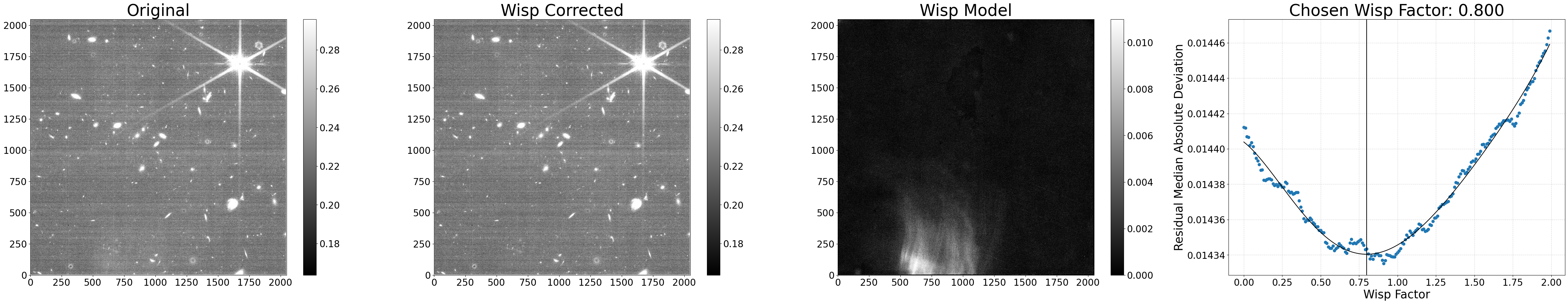
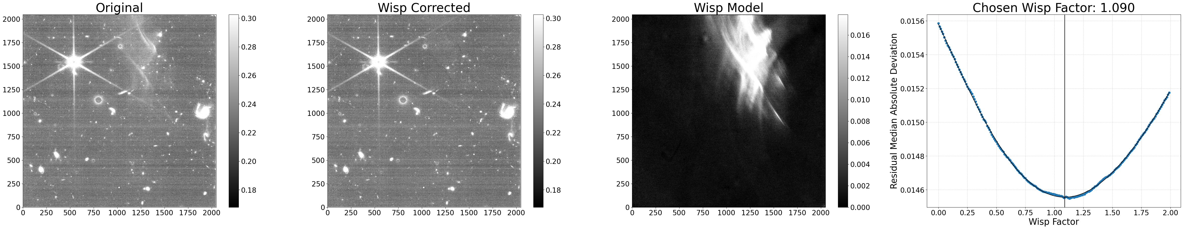
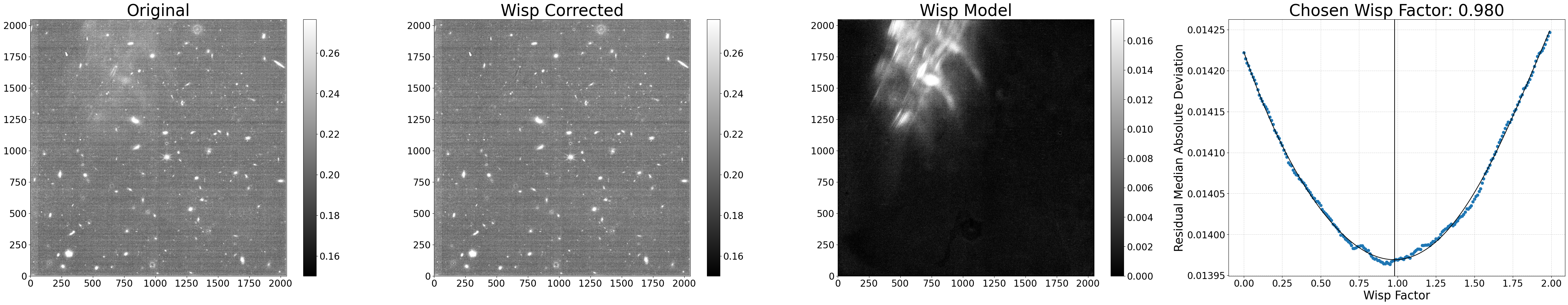
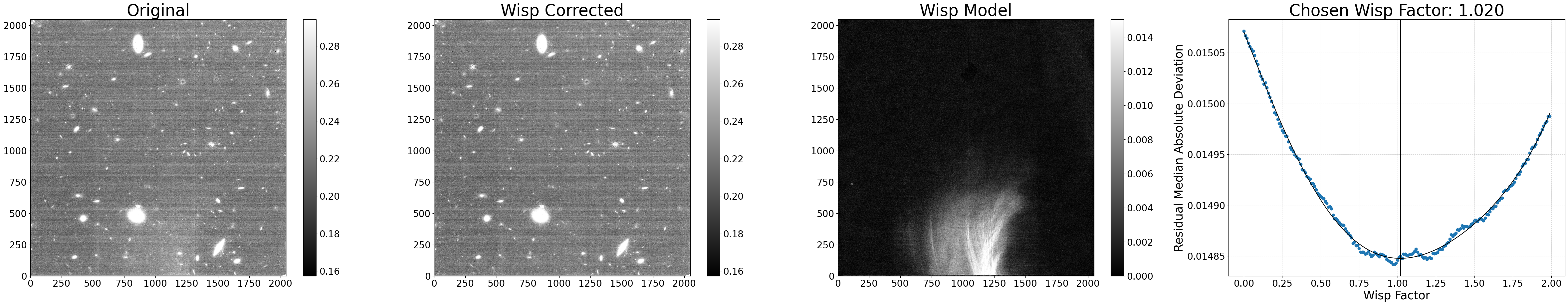
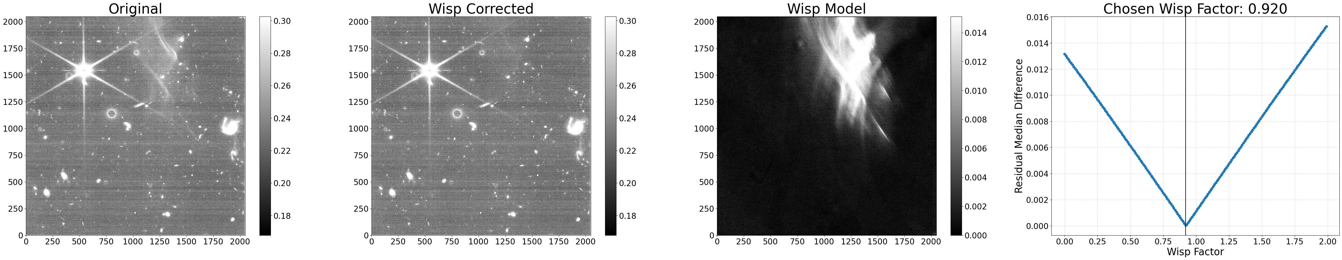
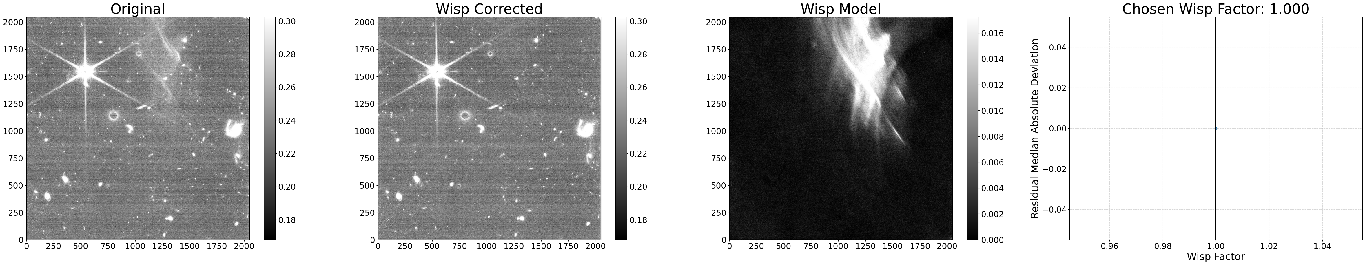
A diagnostic plot showing the original image, the wisp-corrected image, the wisp model subtracted, and a plot showing all of the wisp scale factors tested along with their corresponding residual noise. The factor with the lowest noise is the one applied to the wisp template to generate the wisp model.
Note: calling process_files() rather than process_file() will process the files in parallel. This will save time, but the plots won’t display inline in the notebook.
# Remove wisps from the science data
for file in files:
    results = process_file(file, show_plot=True)
Processing jw01063006004_02101_00005_nrca4_cal.fits
Making segmap for jw01063006004_02101_00005_nrca4_cal.fits
Applying wisp template to jw01063006004_02101_00005_nrca4_cal.fits
Processing complete for jw01063006004_02101_00005_nrca4_cal.fits
Processing jw01063006004_02101_00005_nrcb4_cal.fits
Making segmap for jw01063006004_02101_00005_nrcb4_cal.fits
Applying wisp template to jw01063006004_02101_00005_nrcb4_cal.fits
Processing complete for jw01063006004_02101_00005_nrcb4_cal.fits
Processing jw01063006004_02101_00005_nrca3_cal.fits
Making segmap for jw01063006004_02101_00005_nrca3_cal.fits
Applying wisp template to jw01063006004_02101_00005_nrca3_cal.fits
Processing complete for jw01063006004_02101_00005_nrca3_cal.fits
Processing jw01063006004_02101_00005_nrcb3_cal.fits
Making segmap for jw01063006004_02101_00005_nrcb3_cal.fits
Applying wisp template to jw01063006004_02101_00005_nrcb3_cal.fits
Processing complete for jw01063006004_02101_00005_nrcb3_cal.fits
Python equivalent:
python subtract_wisp.py --files *_cal.fits
Run the wisp subtraction code using custom settings#
In this section, we’ll run the wisp subtraction code using custom settings that may be helpful to optimize the wisp removal. The different settings shown here can be used in combination with those from other examples or as a standalone.
Example 1: New wisp scaling method#
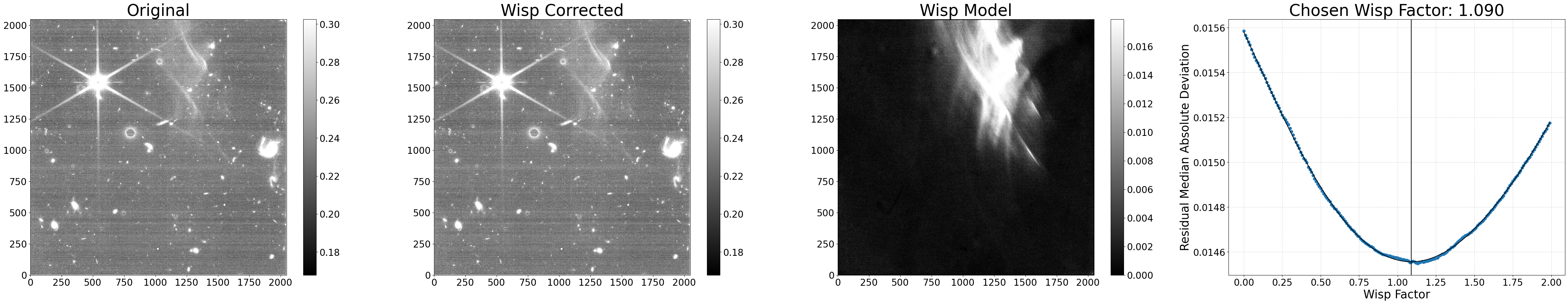
By default, the wisp factor is decided based on that which results in the lowest residual noise. However, the scaling can instead be based on minimizing the overall signal level differences inside and outside the wisp-affected detector regions by setting scale_method='median'. For this scaling method, it’s recommended to also turn off the polynomial fitting on the residuals (poly_degree=0) to simply choose the factor that results in the lowest difference.
During the scaling, residual 1/f noise is corrected by default (correct_rows=True); however, for datasets that have strong e.g. amp offsets or odd-even column residuals, this same correction can be applied in the vertical direction as well (correct_cols=True). Note that these corrections aren’t subtracted in the output file, they are only used to help the wisp scaling procedure.
Below, we perform a new run using these settings.
# Remove wisps using the scaling method
results = process_file('jw01063006004_02101_00005_nrcb4_cal.fits',
                       scale_method='median', poly_degree=0,
                       correct_cols=True, show_plot=True)
Processing jw01063006004_02101_00005_nrcb4_cal.fits
Making segmap for jw01063006004_02101_00005_nrcb4_cal.fits
Applying wisp template to jw01063006004_02101_00005_nrcb4_cal.fits
Processing complete for jw01063006004_02101_00005_nrcb4_cal.fits
Python equivalent: python subtract_wisp.py --files jw01063006004_02101_00005_nrcb4_cal.fits --scale_method median --poly_degree 0 --correct_cols
Sometimes, e.g. for crowded fields, there may not be enough empty regions to scale the wisp properly. In this case, simply subtracting the wisp template with no scaling may provide the best results (scale_wisp=False, or similarly, in python --no-scale_wisp).
Example 2: Data quality flagging#
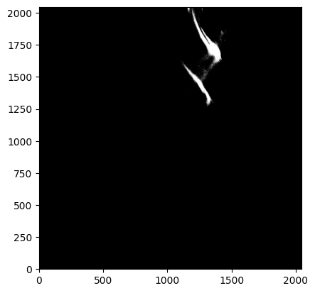
Another option is to flag any pixels with wisp signals above a certain threshold in the image’s data quality array, but not subtract the wisp itself from the science data. This may be useful if you want to ignore these pixels when combining several images into a mosaic or flag them while performing photometry. This can be accomplished by setting flag_wisp_thresh to the chosen wisp signal threshold (units are assumed to be the same as the input file) and sub_wisp=False. The data quality value used here is set by the dq_val parameter.
The default value of dq_val is 1, which is equivalent to the JWST Pipeline DO_NOT_USE flag, and it is ignored by default during image3 drizzling. If you would prefer the pixels to be flagged, but not ignored during that step, another option is using dq_val=1073741824, which is equivalent to the JWST Pipeine OTHER_BAD_PIXEL flag. More details on the various data quality flags can be found here.
# Do not remove wisps, just flag them
results = process_file('jw01063006004_02101_00005_nrcb4_cal.fits',
                       flag_wisp_thresh=0.03, dq_val=1073741824,
                       sub_wisp=False, show_plot=True)
Processing jw01063006004_02101_00005_nrcb4_cal.fits
Making segmap for jw01063006004_02101_00005_nrcb4_cal.fits
Applying wisp template to jw01063006004_02101_00005_nrcb4_cal.fits
Processing complete for jw01063006004_02101_00005_nrcb4_cal.fits
Python equivalent: python subtract_wisp.py --files jw01063006004_02101_00005_nrcb4_cal.fits --flag_wisp_thresh 0.03 --dq_val 1073741824 --no-sub_wisp
Check that the data quality array in this file was updated appropriately
# Check data quality (DQ) array
dq = fits.getdata('jw01063006004_02101_00005_nrcb4_cal_wisp.fits', 'DQ')

# Show  pixels flagged as OTHER_BAD_PIXEL
dq = (dq & 1073741824 != 0).astype(int) # only want to see pixels with dq_val 1073741824
plt.imshow(dq, cmap='gray', origin='lower', vmin=0, vmax=0.1)
<matplotlib.image.AxesImage at 0x7facb6df6ed0>
Example 3: Other misc settings#
This example will show a variety of other settings that may be
useful either used alone or in combination with any of the
other settings shown above. The full list of optional settings
can be seen in the make_segmap() and subtract_wisp() docstrings.
In this example, we’ll do the source-finding on the input image
itself (rather than the corresponding longwave image) by
setting seg_from_lw=False. We’ll increase the source
detection sigma to help avoid flagging the wisp itself, and
we’ll save the resulting segmentation mask by setting
save_segmap=True for inspection. The segmentation mask
filename is the same as the input file, just with the
_seg suffix added.
We’ll also only subtract wisp signals above 0.01 MJy/sr
(min_wisp=0.01). To save a little time, we’ll only test wispscale factors between 0.5 and 1.5 in 0.05 steps.
# Get full list of optional settings for make_segmap() using help(make_segmap)
#
# Use special settings
results = process_file('jw01063006004_02101_00005_nrcb4_cal.fits',
                       seg_from_lw=False, sigma=1.5, save_segmap=True,
                       min_wisp=0.01, factor_min=0.5, factor_max=1.5,
                       factor_step=0.05, show_plot=True)
Processing jw01063006004_02101_00005_nrcb4_cal.fits
Making segmap for jw01063006004_02101_00005_nrcb4_cal.fits
Applying wisp template to jw01063006004_02101_00005_nrcb4_cal.fits
Processing complete for jw01063006004_02101_00005_nrcb4_cal.fits
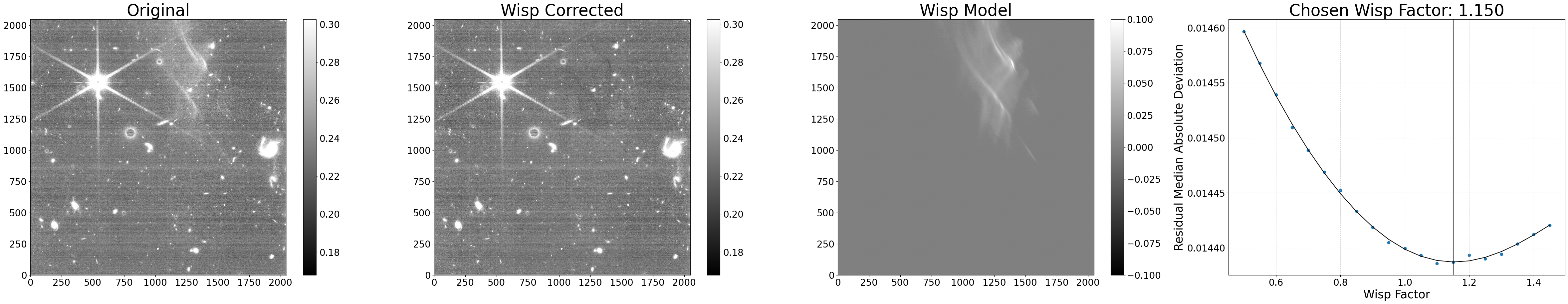
Python equivalent: python subtract_wisp.py --files jw01063006004_02101_00005_nrcb4_cal.fits --no-seg_from_lw --sigma 1.5 --save_segmap --min_wisp 0.01 --factor_min 0.5 --factor_max 1.5 --factor_step 0.05
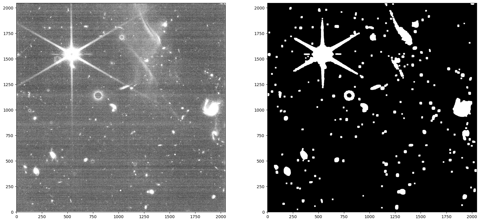
As seen above, these custom settings resulted in an oversubtraction. This is likely due to poor source finding in the wisp region (e.g. the wisp itself being flagged as a source), and why source finding using the longwave image is recommended. We can confirm this by inspecting the generated segmentation map.
data = fits.getdata('jw01063006004_02101_00005_nrcb4_cal.fits')
segmap = fits.getdata('jw01063006004_02101_00005_nrcb4_cal_seg.fits')

# Show the images
fig, axes = plt.subplots(1, 2, figsize=(20, 10))
axes[0].imshow(data, origin='lower', cmap='gray', vmin=0.18, vmax=0.3)
axes[1].imshow(segmap, origin='lower', cmap='gray', vmin=0, vmax=0.1)
<matplotlib.image.AxesImage at 0x7facb7e11a10>
Using custom wisp templates#
This section shows how you can incorporate custom wisp templates while still using the wisp subtraction procedure contained in the main code. This may be useful if you have your own wisp templates or want to apply a manual scale factor to the existing templates.
In this example, we’ll use the existing template, but multiply it by our own scale factor and turn the scaling procedure off (scale_wisp=False) so the code simply applies the wisp model as given. Note that turning off the scaling procedure is not required when using a custom template; users can both provide a custom template and still keep the scaling procedure on. Since the scaling procedure is off in this example, the source finding is irrelevant, and so we can skip the segmap creation function make_segmap() and run subtract_wisp() directly.
# Get the wisp template and apply a manual scale factor
wisp_data = fits.getdata('WISP_NRCB4_F200W_CLEAR.fits') * 1.05

# Process the file with the custom wisp template
results = subtract_wisp('jw01063006004_02101_00005_nrcb4_cal.fits', wisp_data, scale_wisp=False, show_plot=True)
Applying wisp template to jw01063006004_02101_00005_nrcb4_cal.fits
Warning: No segmap data given for jw01063006004_02101_00005_nrcb4_cal.fits. Assuming no sources.
Runing the code in pieces#
In this section, we’ll show how to run the full wisp removal process in pieces. This may be useful to provide more flexibility or when finding the optimal settings to use for your data. We’ll use a variety of custom settings - see the function docstrings for more details.
# The file to process
cal_file = 'jw01063006004_02101_00005_nrcb4_cal.fits'

# The wisp template to use. We'll use a "custom" template again.
wisp_data = fits.getdata('WISP_NRCB4_F200W_CLEAR.fits') * 1.05

# Generate the segmentation map
segmap_data = make_segmap(cal_file, sigma=1.0, npixels=8, dilate_segmap=10)

# Scale and subtract the wisp template
results = subtract_wisp(cal_file, wisp_data=wisp_data, segmap_data=segmap_data, show_plot=True)
Making segmap for jw01063006004_02101_00005_nrcb4_cal.fits
Applying wisp template to jw01063006004_02101_00005_nrcb4_cal.fits
