JWST Using Wavefronts Measured On Orbit

JWST Using Wavefronts Measured On Orbit#

STPSF, formerly knows as WebbPSF, includes code for using the results of in-flight wavefront sensing measurements, by retrieving Optical Path Difference (OPD) files. These can be used to create simulated PSFs appropriate for a given instrument, detector, and time.

This notebook serves as a reference for how to use STPSF to search for and retrieve an OPD file, and explains the contents of this file. It also shows how to load multiple OPD files and plot changes in the wavefront properties over time. It also contains an example case of using an OPD file to create and subtract a simulated PSF from an in-flight image.

Details on the use of STPSF’s in-flight OPDs are given here: https://stpsf.readthedocs.io/en/latest/jwst_measured_opds.html

Author: Marcio Melendez Hernandez
Last Updated: 13 Feb 2025

Index#

Imports and Setup
Finding the measured wavefront near a given date
OPD File description
Delta Wavefront Error Around Time of Observation
Setup a PSF simulation using a particular observation
Trending Wavefront Changes over Time
Wavefront time series and histogram plots
- Table of all OPDs
- Trending Plots
- Plot over a time range
- Load and plot a Single OPD
JWST Simulated PSF Subtraction from in-flight data
- Extract a subarray around source of interest, and measure source location
- Find the source
- Use previous function to set up our simulation
- Use photutils to create our model PSF
- Subtract PSF and create residual image
- PSF properties and differences
Improved IFU Sims

For other STPSF examples: https://stpsf.readthedocs.io/en/latest/more_examples.html

Imports and Setup#

import matplotlib.pylab as plt
import poppy
import numpy as np
import os
import datetime
import tarfile
from urllib.parse import urlparse
import requests

import stpsf

import astropy
from astropy.nddata import Cutout2D
from astropy.visualization import simple_norm
from astropy.io import fits
from astropy.stats import SigmaClip
from astropy.visualization.mpl_normalize import ImageNormalize
from astropy.visualization import LogStretch
from astropy.modeling import models, fitting

import photutils
from photutils.background import Background2D, MedianBackground
from photutils.detection import IRAFStarFinder
from photutils.psf import PSFPhotometry

Matplotlib is building the font cache; this may take a moment.

# Files containing such information as the JWST pupil shape, instrument throughputs, and aperture positions are distributed separately from STPSF.
# To run STPSF, you must download these files and tell STPSF where to find them using the STPSF_PATH environment variable.

# Set environmental variables
os.environ["STPSF_PATH"] = "./data/stpsf-data"

# STPSF Data
stpsf_url = 'https://stsci.box.com/shared/static/kqfolg2bfzqc4mjkgmujo06d3iaymahv.gz'
stpsf_file = './stpsf-data-LATEST.tar.gz'
stpsf_folder = "./data"


def download_file(url, dest_path, timeout=60):
    parsed_url = urlparse(url)
    if parsed_url.scheme not in ["http", "https"]:
        raise ValueError(f"Unsupported URL scheme: {parsed_url.scheme}")

    response = requests.get(url, stream=True, timeout=timeout)
    response.raise_for_status()
    with open(dest_path, "wb") as f:
        for chunk in response.iter_content(chunk_size=8192):
            f.write(chunk)


# Gather stpsf files
stpsfExist = os.path.exists(stpsf_folder)
if not stpsfExist:
    os.makedirs(stpsf_folder)
    download_file(stpsf_url, stpsf_file)
    gzf = tarfile.open(stpsf_file)
    gzf.extractall(stpsf_folder, filter='data')

Finding the measured wavefront near a given date#

nrc = stpsf.NIRCam()
nrc.filter = 'F200W'

nrc.detector = 'NRCB2'
nrc.detector_position = (1024, 1024)

The interpixel capacitance effect is now included for oversampled outputs as well as for the detector-sampled outputs (in the geometric distortion extension). Remember that, in general, the last (“DET_DIST”) FITS extension of the output PSF FITS file are the output data product that most represents the PSF as actually observed on a detector. In any case, there are way to disable any detector effects or to adjust the empirical approximation of charge difussion. For example: nrc.options['charge_diffusion_sigma'] = 0

nrc.options['add_ipc'] = False

output_path = os.getcwd()
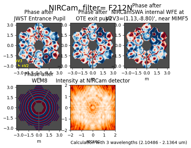
nrc.load_wss_opd_by_date('2022-07-01T00:00:00', plot=True, output_path=output_path)
# choice : string . Default 'closest'
# Method to choose which OPD file to use, e.g. 'before', 'after'

MAST OPD query around UTC: 2022-07-01T00:00:00.000
                        MJD: 59761.0

OPD immediately preceding the given datetime:
	URI:	 mast:JWST/product/R2022063002-NRCA3_FP1-2.fits
	Date (MJD):	 59759.6628
	Delta time:	 -1.3372 days

OPD immediately following the given datetime:
	URI:	 mast:JWST/product/R2022070403-NRCA3_FP1-0.fits
	Date (MJD):	 59761.5484
	Delta time:	 0.5484 days
User requested choosing OPD time closest in time to 2022-07-01T00:00:00.000, which is R2022070403-NRCA3_FP1-0.fits, delta time 0.548 days
Downloading URL https://mast.stsci.edu/api/v0.1/Download/file?uri=mast:JWST/product/R2022070403-NRCA3_FP1-0.fits to /home/runner/work/jdat_notebooks/jdat_notebooks/notebooks/cross_instrument/stpsf_examples/R2022070403-NRCA3_FP1-0.fits ...

 [Done]

Importing and format-converting OPD from /home/runner/work/jdat_notebooks/jdat_notebooks/notebooks/cross_instrument/stpsf_examples/R2022070403-NRCA3_FP1-0.fits
Backing out SI WFE and OTE field dependence at the WF sensing field point (NRCA3_FP1)

../../../_images/e4b70f813d61f4bff22cf7109745ed4c1ffe89fc3c2e14d43386ed26898aabf9.png

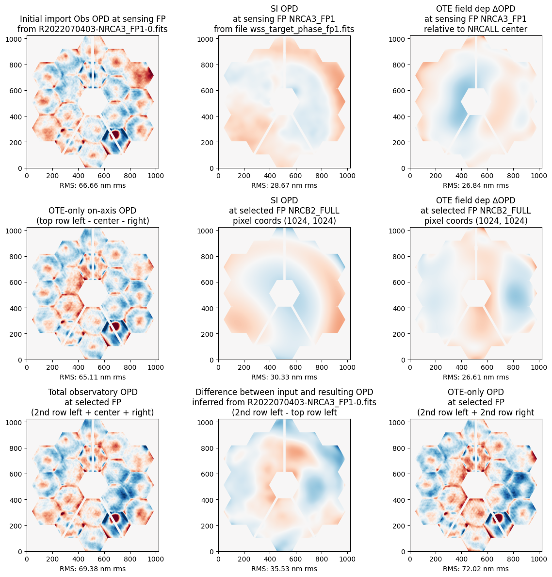
Upper Left: This is the measured OPD as sensed in NIRCam at “field point 1” which is in the upper left corner of NRCA3, relatively close to the center of the NIRCam module. This observatory total OPD measurement includes both the telescope and NIRCam contributions to the WFE.
Upper Middle: This is the wavefront map for the NIRCam portion of the WFE at that field point. This is known from ground calibration test data, not measured in flight.
Upper Right: That NIRCam WFE contribution is subtracted from the total observatory WFE to yield this estimate of the OTE-only portion of the WFE.
Lower Left and Middle: These are models for the field dependence of the OTE OPD between the sensing field point in NRCA3 and the requested field ooint, in this case in NRCB2. This field dependence arises mostly from the figure of the tertiary mirror. These are used to transform the estimated OTE OPD from one field position to another.
Lower Right: This is the resulting estimate for the OTE OPD at the requested field point, in this case in NRCB2.

# What's inside an OPD?
opd_fn = 'R2022070403-NRCA3_FP1-0.fits'
opd = fits.open(os.path.join(output_path, opd_fn))

opd.info()

norm = ImageNormalize(stretch=LogStretch(), vmin=1e-10, vmax=1e-6)
plt.figure(figsize=[10, 18])
for i in range(1, len(opd)):
    plt.subplot(5, 3, i)
    if i == 2:
        plt.imshow(opd[i].data, norm=norm, origin='lower')
    else:
        plt.imshow(opd[i].data, origin='lower')

Filename: /home/runner/work/jdat_notebooks/jdat_notebooks/notebooks/cross_instrument/stpsf_examples/R2022070403-NRCA3_FP1-0.fits
No.    Name      Ver    Type      Cards   Dimensions   Format
PRIMARY       1 PrimaryHDU      23   ()      
RESULT_PHASE    1 ImageHDU       184   (256, 256)   float32   
RESULT_PSF    1 ImageHDU        11   (545, 545)   float32   
EXPECTED      1 ImageHDU        13   (256, 256)   float32   
PUPIL_MASK    1 ImageHDU        11   (256, 256)   int16   
RAW_PSF       1 ImageHDU        14   (256, 256)   float32   
CALC_PSF      1 ImageHDU        12   (546, 546)   float32   
CALC_AMP      1 ImageHDU        12   (256, 256)   float32   
HO_PHASE      1 ImageHDU        12   (256, 256)   float32   
LO_PHASE      1 ImageHDU        12   (256, 256)   float32   
RAW_PSF       1 ImageHDU        14   (256, 256)   float32   
CALC_PSF      1 ImageHDU        12   (546, 546)   float32   
CALC_AMP      1 ImageHDU        12   (256, 256)   float32   
HO_PHASE      1 ImageHDU        12   (256, 256)   float32   
LO_PHASE      1 ImageHDU        12   (256, 256)   float32   

../../../_images/6026cfe91edfbb6ff6e1930130ea8a4d7a172e2746ada84c6cf5a63108211563.png

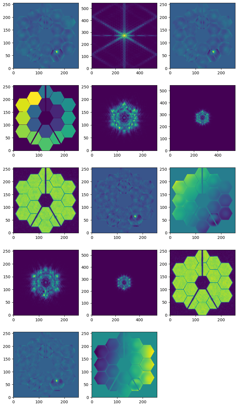
OPD File description#

RESULT_PHASE Image Extension. The FITS file contains a ‘RESULT’ image extension, which is the average of the optical path difference results from all images analyzed together in the phase retrieval
RESULT_PSF Image Extension The FITS file contains a ‘RESULT_PSF’ image extension, which is the PSF computed from the resultant phase by the WAS
EXPECTED Image Extension The FITS file contains an ‘EXPECTED’ image extension, which is the expected optical path difference if the WAS-recommended correction is applied
PUPIL_MASK Image Extension The FITS file contains a ‘PUPIL_MASK’ image extension, which is the pupil mask used to compute the PSF from the resultant phase

The FITS file contains five image extensions for each analyzed input image. In the case of the sensing program, there are 2 images +/-8WL

RAW_PSF Image Extensions For each input image, the Raw PSF extension will contain the raw extracted subimage taken from the calibrated science data
CALC_PSF Image Extensions For each input image, the Calculated PSF extension will contain an image which represents the estimated PSF as calculated by the phase retrieval process
CALC_AMP Image Extension For each input image, the Calculated Amplitude extension will contain an image which represents the estimated pupil amplitude as calculated by the phase retrieval process
HO_PHASE Image Extension For each input image, the High-Order Phase extension will contain an image which represents the retrieved phase information minus the Low-Order (controllable) phase as calculated by the phase retrieval process.
LO_PHASE Image Extension For each input image, the Low-Order Phase extension will contain an image which represents the retrieved controllable phase information as calculated by the phase retrieval process

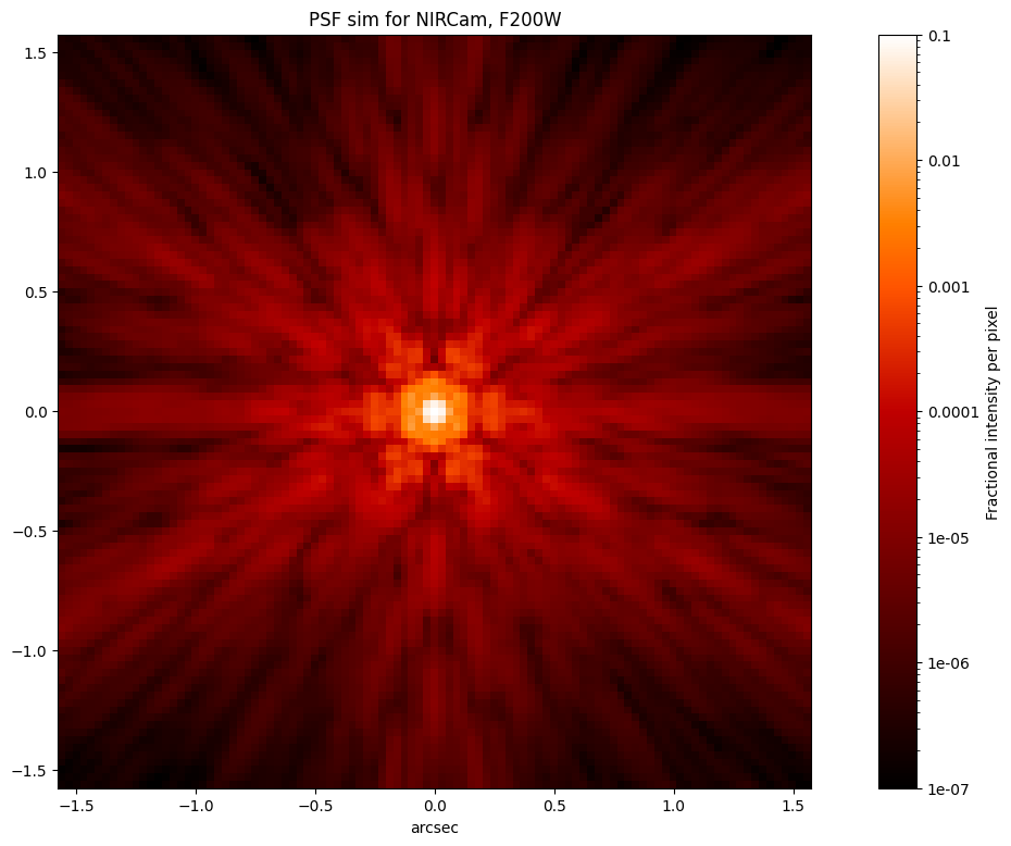
# Let's simulate Webb's PSF from the OPD above
# The PSF below is calculated using the actual 
# as-measured-at-L2 state of the telescope WFE near 
# the requested date, in this case 2022 July 1.
psf = nrc.calc_psf(fov_pixels=101)

plt.figure(figsize=(16, 9))
stpsf.display_psf(psf, ext=1)

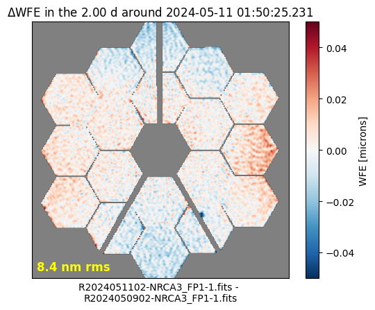
../../../_images/7d82cdc6deb03ce7e62ff265f07b537647118731cfe0278b86391ea7d1c4ec13.png

Delta Wavefront Error Around Time of Observation#

stpsf.trending.delta_wfe_around_time('2024-05-11 01:50:25.231')

Downloading URL https://mast.stsci.edu/api/v0.1/Download/file?uri=mast:JWST/product/R2024050902-NRCA3_FP1-1.fits to data/stpsf-data/MAST_JWST_WSS_OPDs/R2024050902-NRCA3_FP1-1.fits ...

 [Done]

Downloading URL https://mast.stsci.edu/api/v0.1/Download/file?uri=mast:JWST/product/R2024051102-NRCA3_FP1-1.fits to data/stpsf-data/MAST_JWST_WSS_OPDs/R2024051102-NRCA3_FP1-1.fits ...

 [Done]

array([[0., 0., 0., ..., 0., 0., 0.],
       [0., 0., 0., ..., 0., 0., 0.],
       [0., 0., 0., ..., 0., 0., 0.],
       ...,
       [0., 0., 0., ..., 0., 0., 0.],
       [0., 0., 0., ..., 0., 0., 0.],
       [0., 0., 0., ..., 0., 0., 0.]], shape=(256, 256), dtype=float32)

../../../_images/4d2c081e38d1128096b96033ee3a3192bc0af5c5601e10813f9df94530877894.png

Setup a PSF simulation using a particular observation#

def mast_retrieve_files(filename, output_path=None, verbose=False, redownload=False, token=None):
    """Download files from MAST.
    If file is already present locally, the download is skipped and the cached file is used.
    """
    import os
    from requests.exceptions import HTTPError
    from astroquery.mast import Mast
    if token:
        Mast.login(token=token)

    if output_path is None:
        output_path = '.'
    else:
        output_path = output_path

    output_filename = os.path.join(output_path, filename)

    if not os.path.exists(output_path):
        os.mkdir(output_path)

    if os.path.exists(output_filename) and not redownload:
        if verbose:
            print(f"Found file previously downloaded: {filename}")
        return output_filename

    data_uri = f'mast:JWST/product/{filename}'

    # Download the file
    url_path = Mast._portal_api_connection.MAST_DOWNLOAD_URL
    try:
        Mast._download_file(url_path + "?uri=" + data_uri, output_filename)
    except HTTPError as err:
        print(err)
    return output_filename

file = 'jw04500-o056_t012_nircam_f212n-wlm8-nrca3_wfscmb-04.fits'
mast_retrieve_files(file)

Downloading URL https://mast.stsci.edu/api/v0.1/Download/file?uri=mast:JWST/product/jw04500-o056_t012_nircam_f212n-wlm8-nrca3_wfscmb-04.fits to ./jw04500-o056_t012_nircam_f212n-wlm8-nrca3_wfscmb-04.fits ...

 [Done]

'./jw04500-o056_t012_nircam_f212n-wlm8-nrca3_wfscmb-04.fits'

inst = stpsf.setup_sim_to_match_file(file)
position = (512, 1024) # source position
size_pixels = 128 # size in pixels
inst.detector_position = position

single_stpsf_nrc = inst.calc_psf(fov_pixels=size_pixels, display=True)

Setting up sim to match jw04500-o056_t012_nircam_f212n-wlm8-nrca3_wfscmb-04.fits
iterating query, tdelta=3.0

MAST OPD query around UTC: 2024-07-07T13:31:40.751
                        MJD: 60498.56366609954

OPD immediately preceding the given datetime:
	URI:	 mast:JWST/product/O2024070701-NRCA3_FP1-1.fits
	Date (MJD):	 60498.5637
	Delta time:	 -0.0000 days

OPD immediately following the given datetime:
	URI:	 mast:JWST/product/O2024070901-NRCA3_FP1-1.fits
	Date (MJD):	 60500.6226
	Delta time:	 2.0589 days
User requested choosing OPD time closest in time to 2024-07-07T13:31:40.751, which is O2024070701-NRCA3_FP1-1.fits, delta time -0.000 days
Downloading URL https://mast.stsci.edu/api/v0.1/Download/file?uri=mast:JWST/product/O2024070701-NRCA3_FP1-1.fits to data/stpsf-data/MAST_JWST_WSS_OPDs/O2024070701-NRCA3_FP1-1.fits ...

 [Done]

Importing and format-converting OPD from data/stpsf-data/MAST_JWST_WSS_OPDs/O2024070701-NRCA3_FP1-1.fits
Backing out SI WFE and OTE field dependence at the WF sensing field point (NRCA3_FP1)

Configured simulation instrument for:
    Instrument: NIRCam
    Filter: F212N
    Detector: NRCA3
    Apername: NRCA3_FULL
    Det. Pos.: (1024, 1024) 
    Image plane mask: None
    Pupil plane mask: WLM8
    

../../../_images/1b7572cfa7a2595947f5af302aea2bd6ccebc879227f56136e6ee07c008d29bf.png

Trending Wavefront Changes over Time#

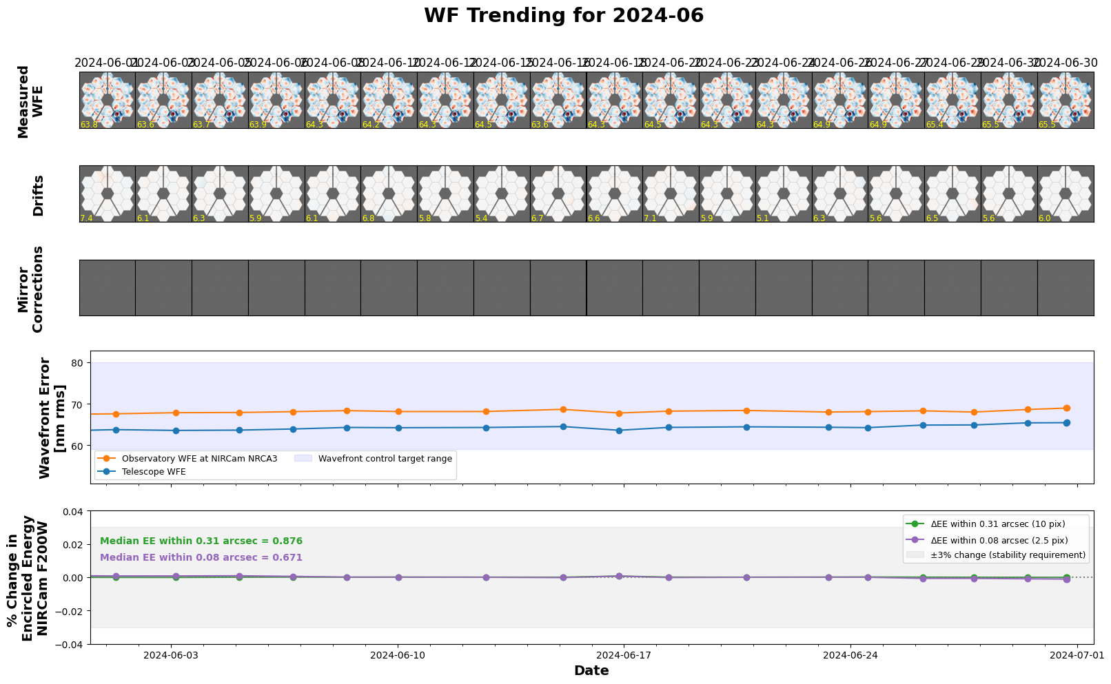
trend_table = stpsf.trending.monthly_trending_plot(2024, 6, verbose=False)

Downloading URL https://mast.stsci.edu/api/v0.1/Download/file?uri=mast:JWST/product/R2024053002-NRCA3_FP1-1.fits to data/stpsf-data/MAST_JWST_WSS_OPDs/R2024053002-NRCA3_FP1-1.fits ...

 [Done]

Downloading URL https://mast.stsci.edu/api/v0.1/Download/file?uri=mast:JWST/product/R2024060102-NRCA3_FP1-1.fits to data/stpsf-data/MAST_JWST_WSS_OPDs/R2024060102-NRCA3_FP1-1.fits ...

 [Done]

Downloading URL https://mast.stsci.edu/api/v0.1/Download/file?uri=mast:JWST/product/R2024060302-NRCA3_FP1-1.fits to data/stpsf-data/MAST_JWST_WSS_OPDs/R2024060302-NRCA3_FP1-1.fits ...

 [Done]

Downloading URL https://mast.stsci.edu/api/v0.1/Download/file?uri=mast:JWST/product/O2024060501-NRCA3_FP1-1.fits to data/stpsf-data/MAST_JWST_WSS_OPDs/O2024060501-NRCA3_FP1-1.fits ...

 [Done]

Downloading URL https://mast.stsci.edu/api/v0.1/Download/file?uri=mast:JWST/product/O2024060602-NRCA3_FP1-1.fits to data/stpsf-data/MAST_JWST_WSS_OPDs/O2024060602-NRCA3_FP1-1.fits ...

 [Done]

Downloading URL https://mast.stsci.edu/api/v0.1/Download/file?uri=mast:JWST/product/O2024060801-NRCA3_FP1-1.fits to data/stpsf-data/MAST_JWST_WSS_OPDs/O2024060801-NRCA3_FP1-1.fits ...

 [Done]

Downloading URL https://mast.stsci.edu/api/v0.1/Download/file?uri=mast:JWST/product/O2024061001-NRCA3_FP1-1.fits to data/stpsf-data/MAST_JWST_WSS_OPDs/O2024061001-NRCA3_FP1-1.fits ...

 [Done]

Downloading URL https://mast.stsci.edu/api/v0.1/Download/file?uri=mast:JWST/product/O2024061301-NRCA3_FP1-1.fits to data/stpsf-data/MAST_JWST_WSS_OPDs/O2024061301-NRCA3_FP1-1.fits ...

 [Done]

Downloading URL https://mast.stsci.edu/api/v0.1/Download/file?uri=mast:JWST/product/O2024061501-NRCA3_FP1-1.fits to data/stpsf-data/MAST_JWST_WSS_OPDs/O2024061501-NRCA3_FP1-1.fits ...

 [Done]

Downloading URL https://mast.stsci.edu/api/v0.1/Download/file?uri=mast:JWST/product/O2024061701-NRCA3_FP1-1.fits to data/stpsf-data/MAST_JWST_WSS_OPDs/O2024061701-NRCA3_FP1-1.fits ...

 [Done]

Downloading URL https://mast.stsci.edu/api/v0.1/Download/file?uri=mast:JWST/product/O2024061801-NRCA3_FP1-1.fits to data/stpsf-data/MAST_JWST_WSS_OPDs/O2024061801-NRCA3_FP1-1.fits ...

 [Done]

Downloading URL https://mast.stsci.edu/api/v0.1/Download/file?uri=mast:JWST/product/O2024062101-NRCA3_FP1-1.fits to data/stpsf-data/MAST_JWST_WSS_OPDs/O2024062101-NRCA3_FP1-1.fits ...

 [Done]

Downloading URL https://mast.stsci.edu/api/v0.1/Download/file?uri=mast:JWST/product/O2024062301-NRCA3_FP1-1.fits to data/stpsf-data/MAST_JWST_WSS_OPDs/O2024062301-NRCA3_FP1-1.fits ...

 [Done]

Downloading URL https://mast.stsci.edu/api/v0.1/Download/file?uri=mast:JWST/product/O2024062401-NRCA3_FP1-1.fits to data/stpsf-data/MAST_JWST_WSS_OPDs/O2024062401-NRCA3_FP1-1.fits ...

 [Done]

Downloading URL https://mast.stsci.edu/api/v0.1/Download/file?uri=mast:JWST/product/O2024062601-NRCA3_FP1-1.fits to data/stpsf-data/MAST_JWST_WSS_OPDs/O2024062601-NRCA3_FP1-1.fits ...

 [Done]

Downloading URL https://mast.stsci.edu/api/v0.1/Download/file?uri=mast:JWST/product/O2024062801-NRCA3_FP1-1.fits to data/stpsf-data/MAST_JWST_WSS_OPDs/O2024062801-NRCA3_FP1-1.fits ...

 [Done]

Downloading URL https://mast.stsci.edu/api/v0.1/Download/file?uri=mast:JWST/product/O2024062901-NRCA3_FP1-1.fits to data/stpsf-data/MAST_JWST_WSS_OPDs/O2024062901-NRCA3_FP1-1.fits ...

 [Done]

../../../_images/84ee7369730048a4ba47c72dc893ed1071839d0b22b2d8a116f8dbf57090417d.png

trend_table

QTable length=17

Date	Filename	WFS Type	RMS WFE (OTE+SI)	RMS WFE (OTE only)	EE(2.5 pix)	EE(10pix)
			nm	nm
str23	str29	str7	float64	float64	float64	float64
2024-05-29T20:28:16.000	R2024053002-NRCA3_FP1-1.fits	Sensing	67.3914750239438	63.3709548042608	0.6719226329668622	0.8764040777120373
2024-06-01T07:23:31.400	R2024060102-NRCA3_FP1-1.fits	Sensing	67.58286840572377	63.77091225744318	0.671716224637393	0.8763351547370711
2024-06-03T03:45:45.700	R2024060302-NRCA3_FP1-1.fits	Sensing	67.85527338663357	63.5824560042632	0.6717277183894746	0.8763239348265368
2024-06-05T02:32:29.000	O2024060501-NRCA3_FP1-1.fits	Sensing	67.89438388454889	63.6531276812743	0.6717958424990571	0.8764245973149776
2024-06-06T18:40:02.000	O2024060602-NRCA3_FP1-1.fits	Sensing	68.10348101293755	63.93035887498094	0.6715480464724863	0.8765101726668102
2024-06-08T10:33:16.100	O2024060801-NRCA3_FP1-1.fits	Sensing	68.35284319652992	64.30054670481502	0.6712569300298153	0.8764032913784519
2024-06-10T00:25:49.700	O2024061001-NRCA3_FP1-1.fits	Sensing	68.12892606755149	64.23481177221457	0.6712435376220324	0.8764395816200582
2024-06-12T17:17:56.200	O2024061301-NRCA3_FP1-1.fits	Sensing	68.13602214356894	64.29193242420945	0.6711962144562941	0.8764299998890757
2024-06-15T02:37:35.900	O2024061501-NRCA3_FP1-1.fits	Sensing	68.65781083419657	64.51686307694686	0.6710741573631243	0.8764018632655044
2024-06-16T20:16:29.500	O2024061701-NRCA3_FP1-1.fits	Sensing	67.77755625455715	63.621440981447485	0.6716471649887765	0.8770141611678653
2024-06-18T08:42:51.200	O2024061801-NRCA3_FP1-1.fits	Sensing	68.22087337229254	64.30479742513361	0.6710999994898569	0.876457100479267
2024-06-20T18:43:56.200	O2024062101-NRCA3_FP1-1.fits	Sensing	68.39046836852398	64.45326019746295	0.6711954538707969	0.8764130078787915
2024-06-23T07:34:47.400	O2024062301-NRCA3_FP1-1.fits	Sensing	68.01667326098666	64.34161990641942	0.6712244606699806	0.8764568399289001
2024-06-24T12:30:24.200	O2024062401-NRCA3_FP1-1.fits	Sensing	68.11333031194278	64.25425350520669	0.671209854304376	0.8765185680175227
2024-06-26T05:34:54.000	O2024062601-NRCA3_FP1-1.fits	Sensing	68.29756935101497	64.86571635421303	0.670749729019986	0.8764423226596338
2024-06-27T19:33:03.300	O2024062801-NRCA3_FP1-1.fits	Sensing	68.0126010582367	64.90436149662717	0.6707506032794925	0.8763846063022834
2024-06-29T11:11:11.900	O2024062901-NRCA3_FP1-1.fits	Sensing	68.61955754982066	65.40644711461798	0.670565698344554	0.8763606492879847

Wavefront time series and histogram plots#

Table of all OPDs#

Retrieve a table of all available OPDs and plot the measurements over time

opdtable = stpsf.mast_wss.retrieve_mast_opd_table()

opdtable = stpsf.mast_wss.deduplicate_opd_table(opdtable)

opdtable

Table length=602

date	date_obs_mjd	visitId	activity	apername	corr_id	fileName	dataURI	wfs_measurement_type	is_post_correction	is_pre_correction
str23	float64	str12	str5	str9	str11	str29	str47	str10	bool	bool
2022-03-11T19:37:04.200	59649.81740972222	V01160001001	02109	NRCA3_FP1	R2022031401	R2022031401-NRCA3_FP1-0.fits	mast:JWST/product/R2022031401-NRCA3_FP1-0.fits	post	True	False
2022-03-12T13:56:12.900	59650.58070486111	V01162001001	02101	NRCA3_FP1	R2022031401	R2022031401-NRCA3_FP1-1.fits	mast:JWST/product/R2022031401-NRCA3_FP1-1.fits	pre	False	False
2022-03-12T19:42:19.800	59650.8210625	V01162006001	02101	NRCA3_FP1	R2022031401	R2022031401-NRCA3_FP1-6.fits	mast:JWST/product/R2022031401-NRCA3_FP1-6.fits	pre	False	False
2022-03-13T02:02:19.300	59651.084945601855	V01162012001	02101	NRCA3_FP1	R2022031303	R2022031303-NRCA3_FP1-1.fits	mast:JWST/product/R2022031303-NRCA3_FP1-1.fits	pre	False	False
2022-03-14T15:44:07.500	59652.65564236111	V01163006001	02107	NRCA3_FP1	R2022031405	R2022031405-NRCA3_FP1-1.fits	mast:JWST/product/R2022031405-NRCA3_FP1-1.fits	post	True	False
2022-03-17T06:50:00.300	59655.284725694444	V01163001001	02101	NRCA3_FP1	R2022032002	R2022032002-NRCA3_FP1-0.fits	mast:JWST/product/R2022032002-NRCA3_FP1-0.fits	pre	False	False
2022-03-17T15:50:41.300	59655.66020023148	V01163003001	02101	NRCA3_FP1	R2022031703	R2022031703-NRCA3_FP1-1.fits	mast:JWST/product/R2022031703-NRCA3_FP1-1.fits	pre	False	False
2022-03-17T22:54:02.800	59655.954199074076	V01163004001	02107	NRCA3_FP1	R2022031801	R2022031801-NRCA3_FP1-1.fits	mast:JWST/product/R2022031801-NRCA3_FP1-1.fits	post	True	False
2022-03-18T05:18:33.700	59656.22122337963	V01163005001	02107	NRCA3_FP1	R2022031902	R2022031902-NRCA3_FP1-0.fits	mast:JWST/product/R2022031902-NRCA3_FP1-0.fits	post	True	False
...	...	...	...	...	...	...	...	...	...	...
2025-01-14T20:48:05.600	60689.86673148148	V06690046001	03104	NRCA1_FP6	O2025011501	O2025011501-NRCA1_FP6-1.fits	mast:JWST/product/O2025011501-NRCA1_FP6-1.fits	pre	False	False
2025-01-19T05:24:01.000	60694.225011574075	V06689097001	03104	NRCA1_FP6	O2025012101	O2025012101-NRCA1_FP6-1.fits	mast:JWST/product/O2025012101-NRCA1_FP6-1.fits	pre	False	False
2025-01-24T05:41:14.900	60699.236978009256	V06691006001	03104	NRCA1_FP6	O2025012501	O2025012501-NRCA1_FP6-1.fits	mast:JWST/product/O2025012501-NRCA1_FP6-1.fits	pre	False	False
2025-01-28T07:08:15.200	60703.29739814815	V06691066001	03104	NRCA1_FP6	R2025012901	R2025012901-NRCA1_FP6-1.fits	mast:JWST/product/R2025012901-NRCA1_FP6-1.fits	pre	False	False
2025-02-01T05:00:34.100	60707.20872800926	V06690166001	03104	NRCA1_FP6	R2025020101	R2025020101-NRCA1_FP6-1.fits	mast:JWST/product/R2025020101-NRCA1_FP6-1.fits	pre	False	True
2025-02-01T05:40:28.500	60707.23644097222	V06690166001	03107	NRCA1_FP6	R2025020102	R2025020102-NRCA1_FP6-1.fits	mast:JWST/product/R2025020102-NRCA1_FP6-1.fits	post	True	False
2025-02-04T20:42:06.700	60710.86257754629	V06691102001	03104	NRCA1_FP6	O2025020501	O2025020501-NRCA1_FP6-1.fits	mast:JWST/product/O2025020501-NRCA1_FP6-1.fits	pre	False	False
2025-02-08T14:13:49.200	60714.592930555555	V06694091001	03104	NRCA1_FP6	O2025020901	O2025020901-NRCA1_FP6-1.fits	mast:JWST/product/O2025020901-NRCA1_FP6-1.fits	pre	False	False
2025-02-12T16:35:29.100	60718.69130902778	V06696083001	03104	NRCA1_FP6	O2025021301	O2025021301-NRCA1_FP6-1.fits	mast:JWST/product/O2025021301-NRCA1_FP6-1.fits	pre	False	False
2025-02-16T18:29:04.100	60722.77018634259	V06694006001	03104	NRCA1_FP6	O2025021701	O2025021701-NRCA1_FP6-1.fits	mast:JWST/product/O2025021701-NRCA1_FP6-1.fits	pre	False	False

Download all the OPDs from the opdtable object. Note that some functions need to have all the OPDs available.

stpsf.mast_wss.download_all_opds(opdtable)

Downloading URL https://mast.stsci.edu/api/v0.1/Download/file?uri=mast:JWST/product/R2022031401-NRCA3_FP1-0.fits to data/stpsf-data/MAST_JWST_WSS_OPDs/R2022031401-NRCA3_FP1-0.fits ...

 [Done]

Downloading URL https://mast.stsci.edu/api/v0.1/Download/file?uri=mast:JWST/product/R2022031401-NRCA3_FP1-1.fits to data/stpsf-data/MAST_JWST_WSS_OPDs/R2022031401-NRCA3_FP1-1.fits ...

 [Done]

Downloading URL https://mast.stsci.edu/api/v0.1/Download/file?uri=mast:JWST/product/R2022031401-NRCA3_FP1-6.fits to data/stpsf-data/MAST_JWST_WSS_OPDs/R2022031401-NRCA3_FP1-6.fits ...

 [Done]

Downloading URL https://mast.stsci.edu/api/v0.1/Download/file?uri=mast:JWST/product/R2022031303-NRCA3_FP1-1.fits to data/stpsf-data/MAST_JWST_WSS_OPDs/R2022031303-NRCA3_FP1-1.fits ...

 [Done]

Downloading URL https://mast.stsci.edu/api/v0.1/Download/file?uri=mast:JWST/product/R2022031405-NRCA3_FP1-1.fits to data/stpsf-data/MAST_JWST_WSS_OPDs/R2022031405-NRCA3_FP1-1.fits ...

 [Done]

Downloading URL https://mast.stsci.edu/api/v0.1/Download/file?uri=mast:JWST/product/R2022032002-NRCA3_FP1-0.fits to data/stpsf-data/MAST_JWST_WSS_OPDs/R2022032002-NRCA3_FP1-0.fits ...

 [Done]

Downloading URL https://mast.stsci.edu/api/v0.1/Download/file?uri=mast:JWST/product/R2022031703-NRCA3_FP1-1.fits to data/stpsf-data/MAST_JWST_WSS_OPDs/R2022031703-NRCA3_FP1-1.fits ...

 [Done]

Downloading URL https://mast.stsci.edu/api/v0.1/Download/file?uri=mast:JWST/product/R2022031801-NRCA3_FP1-1.fits to data/stpsf-data/MAST_JWST_WSS_OPDs/R2022031801-NRCA3_FP1-1.fits ...

 [Done]

Downloading URL https://mast.stsci.edu/api/v0.1/Download/file?uri=mast:JWST/product/R2022031902-NRCA3_FP1-0.fits to data/stpsf-data/MAST_JWST_WSS_OPDs/R2022031902-NRCA3_FP1-0.fits ...

 [Done]

Downloading URL https://mast.stsci.edu/api/v0.1/Download/file?uri=mast:JWST/product/R2022032102-NRCA3_FP1-1.fits to data/stpsf-data/MAST_JWST_WSS_OPDs/R2022032102-NRCA3_FP1-1.fits ...

 [Done]

Downloading URL https://mast.stsci.edu/api/v0.1/Download/file?uri=mast:JWST/product/R2022031902-NRCA3_FP1-2.fits to data/stpsf-data/MAST_JWST_WSS_OPDs/R2022031902-NRCA3_FP1-2.fits ...

 [Done]

Downloading URL https://mast.stsci.edu/api/v0.1/Download/file?uri=mast:JWST/product/R2022031902-NRCA3_FP1-3.fits to data/stpsf-data/MAST_JWST_WSS_OPDs/R2022031902-NRCA3_FP1-3.fits ...

 [Done]

Downloading URL https://mast.stsci.edu/api/v0.1/Download/file?uri=mast:JWST/product/R2022031902-NRCA3_FP1-4.fits to data/stpsf-data/MAST_JWST_WSS_OPDs/R2022031902-NRCA3_FP1-4.fits ...

 [Done]

Downloading URL https://mast.stsci.edu/api/v0.1/Download/file?uri=mast:JWST/product/R2022031902-NRCA3_FP1-5.fits to data/stpsf-data/MAST_JWST_WSS_OPDs/R2022031902-NRCA3_FP1-5.fits ...

 [Done]

Downloading URL https://mast.stsci.edu/api/v0.1/Download/file?uri=mast:JWST/product/R2022031902-NRCA3_FP1-6.fits to data/stpsf-data/MAST_JWST_WSS_OPDs/R2022031902-NRCA3_FP1-6.fits ...

 [Done]

Downloading URL https://mast.stsci.edu/api/v0.1/Download/file?uri=mast:JWST/product/R2022031902-NRCA3_FP1-7.fits to data/stpsf-data/MAST_JWST_WSS_OPDs/R2022031902-NRCA3_FP1-7.fits ...

 [Done]

Downloading URL https://mast.stsci.edu/api/v0.1/Download/file?uri=mast:JWST/product/R2022032002-NRCA3_FP1-1.fits to data/stpsf-data/MAST_JWST_WSS_OPDs/R2022032002-NRCA3_FP1-1.fits ...

 [Done]

Downloading URL https://mast.stsci.edu/api/v0.1/Download/file?uri=mast:JWST/product/R2022032002-NRCA3_FP1-2.fits to data/stpsf-data/MAST_JWST_WSS_OPDs/R2022032002-NRCA3_FP1-2.fits ...

 [Done]

Downloading URL https://mast.stsci.edu/api/v0.1/Download/file?uri=mast:JWST/product/R2022032002-NRCA3_FP1-3.fits to data/stpsf-data/MAST_JWST_WSS_OPDs/R2022032002-NRCA3_FP1-3.fits ...

 [Done]

Downloading URL https://mast.stsci.edu/api/v0.1/Download/file?uri=mast:JWST/product/R2022032002-NRCA3_FP1-4.fits to data/stpsf-data/MAST_JWST_WSS_OPDs/R2022032002-NRCA3_FP1-4.fits ...

 [Done]

Downloading URL https://mast.stsci.edu/api/v0.1/Download/file?uri=mast:JWST/product/R2022032002-NRCA3_FP1-5.fits to data/stpsf-data/MAST_JWST_WSS_OPDs/R2022032002-NRCA3_FP1-5.fits ...

 [Done]

Downloading URL https://mast.stsci.edu/api/v0.1/Download/file?uri=mast:JWST/product/R2022032002-NRCA3_FP1-6.fits to data/stpsf-data/MAST_JWST_WSS_OPDs/R2022032002-NRCA3_FP1-6.fits ...

 [Done]

Downloading URL https://mast.stsci.edu/api/v0.1/Download/file?uri=mast:JWST/product/R2022032002-NRCA3_FP1-7.fits to data/stpsf-data/MAST_JWST_WSS_OPDs/R2022032002-NRCA3_FP1-7.fits ...

 [Done]

Downloading URL https://mast.stsci.edu/api/v0.1/Download/file?uri=mast:JWST/product/R2022032005-NRCA3_FP1-1.fits to data/stpsf-data/MAST_JWST_WSS_OPDs/R2022032005-NRCA3_FP1-1.fits ...

 [Done]

Downloading URL https://mast.stsci.edu/api/v0.1/Download/file?uri=mast:JWST/product/O2022032401-NRCA3_FP1-1.fits to data/stpsf-data/MAST_JWST_WSS_OPDs/O2022032401-NRCA3_FP1-1.fits ...

 [Done]

Downloading URL https://mast.stsci.edu/api/v0.1/Download/file?uri=mast:JWST/product/O2022032501-NRCA3_FP1-1.fits to data/stpsf-data/MAST_JWST_WSS_OPDs/O2022032501-NRCA3_FP1-1.fits ...

 [Done]

Downloading URL https://mast.stsci.edu/api/v0.1/Download/file?uri=mast:JWST/product/O2022032601-NRCA3_FP1-1.fits to data/stpsf-data/MAST_JWST_WSS_OPDs/O2022032601-NRCA3_FP1-1.fits ...

 [Done]

Downloading URL https://mast.stsci.edu/api/v0.1/Download/file?uri=mast:JWST/product/O2022032601-NRCA3_FP1-3.fits to data/stpsf-data/MAST_JWST_WSS_OPDs/O2022032601-NRCA3_FP1-3.fits ...

 [Done]

Downloading URL https://mast.stsci.edu/api/v0.1/Download/file?uri=mast:JWST/product/R2022032603-NRCA3_FP1-1.fits to data/stpsf-data/MAST_JWST_WSS_OPDs/R2022032603-NRCA3_FP1-1.fits ...

 [Done]

Downloading URL https://mast.stsci.edu/api/v0.1/Download/file?uri=mast:JWST/product/R2022032603-NRCA3_FP1-2.fits to data/stpsf-data/MAST_JWST_WSS_OPDs/R2022032603-NRCA3_FP1-2.fits ...

 [Done]

Downloading URL https://mast.stsci.edu/api/v0.1/Download/file?uri=mast:JWST/product/R2022032701-NRCA3_FP1-1.fits to data/stpsf-data/MAST_JWST_WSS_OPDs/R2022032701-NRCA3_FP1-1.fits ...

 [Done]

Downloading URL https://mast.stsci.edu/api/v0.1/Download/file?uri=mast:JWST/product/R2022032701-NRCA3_FP1-2.fits to data/stpsf-data/MAST_JWST_WSS_OPDs/R2022032701-NRCA3_FP1-2.fits ...

 [Done]

Downloading URL https://mast.stsci.edu/api/v0.1/Download/file?uri=mast:JWST/product/R2022032801-NRCA3_FP1-1.fits to data/stpsf-data/MAST_JWST_WSS_OPDs/R2022032801-NRCA3_FP1-1.fits ...

 [Done]

Downloading URL https://mast.stsci.edu/api/v0.1/Download/file?uri=mast:JWST/product/R2022032801-NRCA3_FP1-2.fits to data/stpsf-data/MAST_JWST_WSS_OPDs/R2022032801-NRCA3_FP1-2.fits ...

 [Done]

Downloading URL https://mast.stsci.edu/api/v0.1/Download/file?uri=mast:JWST/product/R2022032901-NRCA3_FP1-1.fits to data/stpsf-data/MAST_JWST_WSS_OPDs/R2022032901-NRCA3_FP1-1.fits ...

 [Done]

Downloading URL https://mast.stsci.edu/api/v0.1/Download/file?uri=mast:JWST/product/R2022032901-NRCA3_FP1-2.fits to data/stpsf-data/MAST_JWST_WSS_OPDs/R2022032901-NRCA3_FP1-2.fits ...

 [Done]

Downloading URL https://mast.stsci.edu/api/v0.1/Download/file?uri=mast:JWST/product/R2022033101-NRCA3_FP1-1.fits to data/stpsf-data/MAST_JWST_WSS_OPDs/R2022033101-NRCA3_FP1-1.fits ...

 [Done]

Downloading URL https://mast.stsci.edu/api/v0.1/Download/file?uri=mast:JWST/product/R2022033101-NRCA3_FP1-2.fits to data/stpsf-data/MAST_JWST_WSS_OPDs/R2022033101-NRCA3_FP1-2.fits ...

 [Done]

Downloading URL https://mast.stsci.edu/api/v0.1/Download/file?uri=mast:JWST/product/R2022040101-NRCA3_FP1-1.fits to data/stpsf-data/MAST_JWST_WSS_OPDs/R2022040101-NRCA3_FP1-1.fits ...

 [Done]

Downloading URL https://mast.stsci.edu/api/v0.1/Download/file?uri=mast:JWST/product/R2022040101-NRCA3_FP1-2.fits to data/stpsf-data/MAST_JWST_WSS_OPDs/R2022040101-NRCA3_FP1-2.fits ...

 [Done]

Downloading URL https://mast.stsci.edu/api/v0.1/Download/file?uri=mast:JWST/product/R2022040201-NRCA3_FP1-1.fits to data/stpsf-data/MAST_JWST_WSS_OPDs/R2022040201-NRCA3_FP1-1.fits ...

 [Done]

Downloading URL https://mast.stsci.edu/api/v0.1/Download/file?uri=mast:JWST/product/R2022040201-NRCA3_FP1-2.fits to data/stpsf-data/MAST_JWST_WSS_OPDs/R2022040201-NRCA3_FP1-2.fits ...

 [Done]

Downloading URL https://mast.stsci.edu/api/v0.1/Download/file?uri=mast:JWST/product/R2022040301-NRCA3_FP1-1.fits to data/stpsf-data/MAST_JWST_WSS_OPDs/R2022040301-NRCA3_FP1-1.fits ...

 [Done]

Downloading URL https://mast.stsci.edu/api/v0.1/Download/file?uri=mast:JWST/product/R2022040301-NRCA3_FP1-2.fits to data/stpsf-data/MAST_JWST_WSS_OPDs/R2022040301-NRCA3_FP1-2.fits ...

 [Done]

Downloading URL https://mast.stsci.edu/api/v0.1/Download/file?uri=mast:JWST/product/R2022040401-NRCA3_FP1-1.fits to data/stpsf-data/MAST_JWST_WSS_OPDs/R2022040401-NRCA3_FP1-1.fits ...

 [Done]

Downloading URL https://mast.stsci.edu/api/v0.1/Download/file?uri=mast:JWST/product/R2022040401-NRCA3_FP1-2.fits to data/stpsf-data/MAST_JWST_WSS_OPDs/R2022040401-NRCA3_FP1-2.fits ...

 [Done]

Downloading URL https://mast.stsci.edu/api/v0.1/Download/file?uri=mast:JWST/product/R2022040501-NRCA3_FP1-1.fits to data/stpsf-data/MAST_JWST_WSS_OPDs/R2022040501-NRCA3_FP1-1.fits ...

 [Done]

Downloading URL https://mast.stsci.edu/api/v0.1/Download/file?uri=mast:JWST/product/R2022040501-NRCA3_FP1-2.fits to data/stpsf-data/MAST_JWST_WSS_OPDs/R2022040501-NRCA3_FP1-2.fits ...

 [Done]

Downloading URL https://mast.stsci.edu/api/v0.1/Download/file?uri=mast:JWST/product/R2022040602-NRCA3_FP1-1.fits to data/stpsf-data/MAST_JWST_WSS_OPDs/R2022040602-NRCA3_FP1-1.fits ...

 [Done]

Downloading URL https://mast.stsci.edu/api/v0.1/Download/file?uri=mast:JWST/product/R2022040602-NRCA3_FP1-2.fits to data/stpsf-data/MAST_JWST_WSS_OPDs/R2022040602-NRCA3_FP1-2.fits ...

 [Done]

Downloading URL https://mast.stsci.edu/api/v0.1/Download/file?uri=mast:JWST/product/R2022040702-NRCA3_FP1-1.fits to data/stpsf-data/MAST_JWST_WSS_OPDs/R2022040702-NRCA3_FP1-1.fits ...

 [Done]

Downloading URL https://mast.stsci.edu/api/v0.1/Download/file?uri=mast:JWST/product/R2022040702-NRCA3_FP1-2.fits to data/stpsf-data/MAST_JWST_WSS_OPDs/R2022040702-NRCA3_FP1-2.fits ...

 [Done]

Downloading URL https://mast.stsci.edu/api/v0.1/Download/file?uri=mast:JWST/product/R2022040802-NRCA3_FP1-1.fits to data/stpsf-data/MAST_JWST_WSS_OPDs/R2022040802-NRCA3_FP1-1.fits ...

 [Done]

Downloading URL https://mast.stsci.edu/api/v0.1/Download/file?uri=mast:JWST/product/R2022040802-NRCA3_FP1-2.fits to data/stpsf-data/MAST_JWST_WSS_OPDs/R2022040802-NRCA3_FP1-2.fits ...

 [Done]

Downloading URL https://mast.stsci.edu/api/v0.1/Download/file?uri=mast:JWST/product/R2022040902-NRCA3_FP1-1.fits to data/stpsf-data/MAST_JWST_WSS_OPDs/R2022040902-NRCA3_FP1-1.fits ...

 [Done]

Downloading URL https://mast.stsci.edu/api/v0.1/Download/file?uri=mast:JWST/product/R2022040902-NRCA3_FP1-2.fits to data/stpsf-data/MAST_JWST_WSS_OPDs/R2022040902-NRCA3_FP1-2.fits ...

 [Done]

Downloading URL https://mast.stsci.edu/api/v0.1/Download/file?uri=mast:JWST/product/R2022041101-NRCA3_FP1-1.fits to data/stpsf-data/MAST_JWST_WSS_OPDs/R2022041101-NRCA3_FP1-1.fits ...

 [Done]

Downloading URL https://mast.stsci.edu/api/v0.1/Download/file?uri=mast:JWST/product/R2022041101-NRCA3_FP1-2.fits to data/stpsf-data/MAST_JWST_WSS_OPDs/R2022041101-NRCA3_FP1-2.fits ...

 [Done]

Downloading URL https://mast.stsci.edu/api/v0.1/Download/file?uri=mast:JWST/product/R2022041201-NRCA3_FP1-1.fits to data/stpsf-data/MAST_JWST_WSS_OPDs/R2022041201-NRCA3_FP1-1.fits ...

 [Done]

Downloading URL https://mast.stsci.edu/api/v0.1/Download/file?uri=mast:JWST/product/R2022041201-NRCA3_FP1-2.fits to data/stpsf-data/MAST_JWST_WSS_OPDs/R2022041201-NRCA3_FP1-2.fits ...

 [Done]

Downloading URL https://mast.stsci.edu/api/v0.1/Download/file?uri=mast:JWST/product/R2022041301-NRCA3_FP1-1.fits to data/stpsf-data/MAST_JWST_WSS_OPDs/R2022041301-NRCA3_FP1-1.fits ...

 [Done]

Downloading URL https://mast.stsci.edu/api/v0.1/Download/file?uri=mast:JWST/product/R2022041301-NRCA3_FP1-2.fits to data/stpsf-data/MAST_JWST_WSS_OPDs/R2022041301-NRCA3_FP1-2.fits ...

 [Done]

Downloading URL https://mast.stsci.edu/api/v0.1/Download/file?uri=mast:JWST/product/R2022041402-NRCA3_FP1-1.fits to data/stpsf-data/MAST_JWST_WSS_OPDs/R2022041402-NRCA3_FP1-1.fits ...

 [Done]

Downloading URL https://mast.stsci.edu/api/v0.1/Download/file?uri=mast:JWST/product/R2022041402-NRCA3_FP1-2.fits to data/stpsf-data/MAST_JWST_WSS_OPDs/R2022041402-NRCA3_FP1-2.fits ...

 [Done]

Downloading URL https://mast.stsci.edu/api/v0.1/Download/file?uri=mast:JWST/product/O2022041404-NRCA3_FP1-1.fits to data/stpsf-data/MAST_JWST_WSS_OPDs/O2022041404-NRCA3_FP1-1.fits ...

 [Done]

Downloading URL https://mast.stsci.edu/api/v0.1/Download/file?uri=mast:JWST/product/O2022041501-NRCA3_FP1-1.fits to data/stpsf-data/MAST_JWST_WSS_OPDs/O2022041501-NRCA3_FP1-1.fits ...

 [Done]

Downloading URL https://mast.stsci.edu/api/v0.1/Download/file?uri=mast:JWST/product/R2022041504-NRCA3_FP1-1.fits to data/stpsf-data/MAST_JWST_WSS_OPDs/R2022041504-NRCA3_FP1-1.fits ...

 [Done]

Downloading URL https://mast.stsci.edu/api/v0.1/Download/file?uri=mast:JWST/product/R2022041506-NRCA3_FP1-1.fits to data/stpsf-data/MAST_JWST_WSS_OPDs/R2022041506-NRCA3_FP1-1.fits ...

 [Done]

Downloading URL https://mast.stsci.edu/api/v0.1/Download/file?uri=mast:JWST/product/R2022041506-NRCA3_FP1-2.fits to data/stpsf-data/MAST_JWST_WSS_OPDs/R2022041506-NRCA3_FP1-2.fits ...

 [Done]

Downloading URL https://mast.stsci.edu/api/v0.1/Download/file?uri=mast:JWST/product/O2022041601-NRCA3_FP1-1.fits to data/stpsf-data/MAST_JWST_WSS_OPDs/O2022041601-NRCA3_FP1-1.fits ...

 [Done]

Downloading URL https://mast.stsci.edu/api/v0.1/Download/file?uri=mast:JWST/product/R2022041905-NRCA3_FP1-1.fits to data/stpsf-data/MAST_JWST_WSS_OPDs/R2022041905-NRCA3_FP1-1.fits ...

 [Done]

Downloading URL https://mast.stsci.edu/api/v0.1/Download/file?uri=mast:JWST/product/R2022041906-NRCA3_FP1-1.fits to data/stpsf-data/MAST_JWST_WSS_OPDs/R2022041906-NRCA3_FP1-1.fits ...

 [Done]

Downloading URL https://mast.stsci.edu/api/v0.1/Download/file?uri=mast:JWST/product/R2022041801-NRCA3_FP1-2.fits to data/stpsf-data/MAST_JWST_WSS_OPDs/R2022041801-NRCA3_FP1-2.fits ...

 [Done]

Downloading URL https://mast.stsci.edu/api/v0.1/Download/file?uri=mast:JWST/product/R2022041801-NRCA3_FP1-3.fits to data/stpsf-data/MAST_JWST_WSS_OPDs/R2022041801-NRCA3_FP1-3.fits ...

 [Done]

Downloading URL https://mast.stsci.edu/api/v0.1/Download/file?uri=mast:JWST/product/R2022041801-NRCA3_FP1-4.fits to data/stpsf-data/MAST_JWST_WSS_OPDs/R2022041801-NRCA3_FP1-4.fits ...

 [Done]

Downloading URL https://mast.stsci.edu/api/v0.1/Download/file?uri=mast:JWST/product/R2022041801-NRCA3_FP1-5.fits to data/stpsf-data/MAST_JWST_WSS_OPDs/R2022041801-NRCA3_FP1-5.fits ...

 [Done]

Downloading URL https://mast.stsci.edu/api/v0.1/Download/file?uri=mast:JWST/product/R2022041801-NRCA3_FP1-6.fits to data/stpsf-data/MAST_JWST_WSS_OPDs/R2022041801-NRCA3_FP1-6.fits ...

 [Done]

Downloading URL https://mast.stsci.edu/api/v0.1/Download/file?uri=mast:JWST/product/R2022041801-NRCA3_FP1-7.fits to data/stpsf-data/MAST_JWST_WSS_OPDs/R2022041801-NRCA3_FP1-7.fits ...

 [Done]

Downloading URL https://mast.stsci.edu/api/v0.1/Download/file?uri=mast:JWST/product/R2022041801-NRCA3_FP1-8.fits to data/stpsf-data/MAST_JWST_WSS_OPDs/R2022041801-NRCA3_FP1-8.fits ...

 [Done]

Downloading URL https://mast.stsci.edu/api/v0.1/Download/file?uri=mast:JWST/product/R2022041902-NRCA3_FP1-1.fits to data/stpsf-data/MAST_JWST_WSS_OPDs/R2022041902-NRCA3_FP1-1.fits ...

 [Done]

Downloading URL https://mast.stsci.edu/api/v0.1/Download/file?uri=mast:JWST/product/R2022041902-NRCA3_FP1-2.fits to data/stpsf-data/MAST_JWST_WSS_OPDs/R2022041902-NRCA3_FP1-2.fits ...

 [Done]

Downloading URL https://mast.stsci.edu/api/v0.1/Download/file?uri=mast:JWST/product/R2022041902-NRCA3_FP1-3.fits to data/stpsf-data/MAST_JWST_WSS_OPDs/R2022041902-NRCA3_FP1-3.fits ...

 [Done]

Downloading URL https://mast.stsci.edu/api/v0.1/Download/file?uri=mast:JWST/product/R2022041902-NRCA3_FP1-4.fits to data/stpsf-data/MAST_JWST_WSS_OPDs/R2022041902-NRCA3_FP1-4.fits ...

 [Done]

Downloading URL https://mast.stsci.edu/api/v0.1/Download/file?uri=mast:JWST/product/R2022041902-NRCA3_FP1-5.fits to data/stpsf-data/MAST_JWST_WSS_OPDs/R2022041902-NRCA3_FP1-5.fits ...

 [Done]

Downloading URL https://mast.stsci.edu/api/v0.1/Download/file?uri=mast:JWST/product/R2022041902-NRCA3_FP1-6.fits to data/stpsf-data/MAST_JWST_WSS_OPDs/R2022041902-NRCA3_FP1-6.fits ...

 [Done]

Downloading URL https://mast.stsci.edu/api/v0.1/Download/file?uri=mast:JWST/product/R2022041902-NRCA3_FP1-7.fits to data/stpsf-data/MAST_JWST_WSS_OPDs/R2022041902-NRCA3_FP1-7.fits ...

 [Done]

Downloading URL https://mast.stsci.edu/api/v0.1/Download/file?uri=mast:JWST/product/R2022041902-NRCA3_FP1-8.fits to data/stpsf-data/MAST_JWST_WSS_OPDs/R2022041902-NRCA3_FP1-8.fits ...

 [Done]

Downloading URL https://mast.stsci.edu/api/v0.1/Download/file?uri=mast:JWST/product/R2022041905-NRCA3_FP1-2.fits to data/stpsf-data/MAST_JWST_WSS_OPDs/R2022041905-NRCA3_FP1-2.fits ...

 [Done]

Downloading URL https://mast.stsci.edu/api/v0.1/Download/file?uri=mast:JWST/product/R2022042302-NRCA3_FP1-1.fits to data/stpsf-data/MAST_JWST_WSS_OPDs/R2022042302-NRCA3_FP1-1.fits ...

 [Done]

Downloading URL https://mast.stsci.edu/api/v0.1/Download/file?uri=mast:JWST/product/R2022042302-NRCA3_FP1-2.fits to data/stpsf-data/MAST_JWST_WSS_OPDs/R2022042302-NRCA3_FP1-2.fits ...

 [Done]

Downloading URL https://mast.stsci.edu/api/v0.1/Download/file?uri=mast:JWST/product/R2022042601-NRCA3_FP1-1.fits to data/stpsf-data/MAST_JWST_WSS_OPDs/R2022042601-NRCA3_FP1-1.fits ...

 [Done]

Downloading URL https://mast.stsci.edu/api/v0.1/Download/file?uri=mast:JWST/product/R2022042601-NRCA3_FP1-2.fits to data/stpsf-data/MAST_JWST_WSS_OPDs/R2022042601-NRCA3_FP1-2.fits ...

 [Done]

Downloading URL https://mast.stsci.edu/api/v0.1/Download/file?uri=mast:JWST/product/R2022042901-NRCA3_FP1-1.fits to data/stpsf-data/MAST_JWST_WSS_OPDs/R2022042901-NRCA3_FP1-1.fits ...

 [Done]

Downloading URL https://mast.stsci.edu/api/v0.1/Download/file?uri=mast:JWST/product/R2022043002-NRCA3_FP1-1.fits to data/stpsf-data/MAST_JWST_WSS_OPDs/R2022043002-NRCA3_FP1-1.fits ...

 [Done]

Downloading URL https://mast.stsci.edu/api/v0.1/Download/file?uri=mast:JWST/product/R2022050302-NRCA3_FP1-1.fits to data/stpsf-data/MAST_JWST_WSS_OPDs/R2022050302-NRCA3_FP1-1.fits ...

 [Done]

Downloading URL https://mast.stsci.edu/api/v0.1/Download/file?uri=mast:JWST/product/R2022050504-NRCA3_FP1-1.fits to data/stpsf-data/MAST_JWST_WSS_OPDs/R2022050504-NRCA3_FP1-1.fits ...

 [Done]

Downloading URL https://mast.stsci.edu/api/v0.1/Download/file?uri=mast:JWST/product/R2022050504-NRCA3_FP1-2.fits to data/stpsf-data/MAST_JWST_WSS_OPDs/R2022050504-NRCA3_FP1-2.fits ...

 [Done]

Downloading URL https://mast.stsci.edu/api/v0.1/Download/file?uri=mast:JWST/product/R2022050802-NRCA3_FP1-1.fits to data/stpsf-data/MAST_JWST_WSS_OPDs/R2022050802-NRCA3_FP1-1.fits ...

 [Done]

Downloading URL https://mast.stsci.edu/api/v0.1/Download/file?uri=mast:JWST/product/R2022050802-NRCA3_FP1-2.fits to data/stpsf-data/MAST_JWST_WSS_OPDs/R2022050802-NRCA3_FP1-2.fits ...

 [Done]

Downloading URL https://mast.stsci.edu/api/v0.1/Download/file?uri=mast:JWST/product/R2022050902-NRCA3_FP1-1.fits to data/stpsf-data/MAST_JWST_WSS_OPDs/R2022050902-NRCA3_FP1-1.fits ...

 [Done]

Downloading URL https://mast.stsci.edu/api/v0.1/Download/file?uri=mast:JWST/product/R2022051102-NRCA3_FP1-21.fits to data/stpsf-data/MAST_JWST_WSS_OPDs/R2022051102-NRCA3_FP1-21.fits ...

 [Done]

Downloading URL https://mast.stsci.edu/api/v0.1/Download/file?uri=mast:JWST/product/R2022051102-NRCA3_FP1-22.fits to data/stpsf-data/MAST_JWST_WSS_OPDs/R2022051102-NRCA3_FP1-22.fits ...

 [Done]

Downloading URL https://mast.stsci.edu/api/v0.1/Download/file?uri=mast:JWST/product/R2022051102-NRCA3_FP1-6.fits to data/stpsf-data/MAST_JWST_WSS_OPDs/R2022051102-NRCA3_FP1-6.fits ...

 [Done]

Downloading URL https://mast.stsci.edu/api/v0.1/Download/file?uri=mast:JWST/product/R2022051309-NRCA3_FP1-1.fits to data/stpsf-data/MAST_JWST_WSS_OPDs/R2022051309-NRCA3_FP1-1.fits ...

 [Done]

Downloading URL https://mast.stsci.edu/api/v0.1/Download/file?uri=mast:JWST/product/O2022052001-NRCA3_FP1-0.fits to data/stpsf-data/MAST_JWST_WSS_OPDs/O2022052001-NRCA3_FP1-0.fits ...

 [Done]

Downloading URL https://mast.stsci.edu/api/v0.1/Download/file?uri=mast:JWST/product/R2022052301-NRCA3_FP1-56.fits to data/stpsf-data/MAST_JWST_WSS_OPDs/R2022052301-NRCA3_FP1-56.fits ...

 [Done]

Downloading URL https://mast.stsci.edu/api/v0.1/Download/file?uri=mast:JWST/product/R2022052301-NRCA3_FP1-57.fits to data/stpsf-data/MAST_JWST_WSS_OPDs/R2022052301-NRCA3_FP1-57.fits ...

 [Done]

Downloading URL https://mast.stsci.edu/api/v0.1/Download/file?uri=mast:JWST/product/O2022052501-NRCA3_FP1-59.fits to data/stpsf-data/MAST_JWST_WSS_OPDs/O2022052501-NRCA3_FP1-59.fits ...

 [Done]

Downloading URL https://mast.stsci.edu/api/v0.1/Download/file?uri=mast:JWST/product/R2022052701-NRCA3_FP1-0.fits to data/stpsf-data/MAST_JWST_WSS_OPDs/R2022052701-NRCA3_FP1-0.fits ...

 [Done]

Downloading URL https://mast.stsci.edu/api/v0.1/Download/file?uri=mast:JWST/product/R2022052701-NRCA3_FP1-1.fits to data/stpsf-data/MAST_JWST_WSS_OPDs/R2022052701-NRCA3_FP1-1.fits ...

 [Done]

Downloading URL https://mast.stsci.edu/api/v0.1/Download/file?uri=mast:JWST/product/R2022060101-NRCA3_FP1-1.fits to data/stpsf-data/MAST_JWST_WSS_OPDs/R2022060101-NRCA3_FP1-1.fits ...

 [Done]

Downloading URL https://mast.stsci.edu/api/v0.1/Download/file?uri=mast:JWST/product/R2022060101-NRCA3_FP1-2.fits to data/stpsf-data/MAST_JWST_WSS_OPDs/R2022060101-NRCA3_FP1-2.fits ...

 [Done]

Downloading URL https://mast.stsci.edu/api/v0.1/Download/file?uri=mast:JWST/product/R2022060103-NRCA3_FP1-1.fits to data/stpsf-data/MAST_JWST_WSS_OPDs/R2022060103-NRCA3_FP1-1.fits ...

 [Done]

Downloading URL https://mast.stsci.edu/api/v0.1/Download/file?uri=mast:JWST/product/R2022060402-NRCA3_FP1-1.fits to data/stpsf-data/MAST_JWST_WSS_OPDs/R2022060402-NRCA3_FP1-1.fits ...

 [Done]

Downloading URL https://mast.stsci.edu/api/v0.1/Download/file?uri=mast:JWST/product/R2022060602-NRCA3_FP1-1.fits to data/stpsf-data/MAST_JWST_WSS_OPDs/R2022060602-NRCA3_FP1-1.fits ...

 [Done]

Downloading URL https://mast.stsci.edu/api/v0.1/Download/file?uri=mast:JWST/product/R2022060802-NRCA3_FP1-1.fits to data/stpsf-data/MAST_JWST_WSS_OPDs/R2022060802-NRCA3_FP1-1.fits ...

 [Done]

Downloading URL https://mast.stsci.edu/api/v0.1/Download/file?uri=mast:JWST/product/R2022060802-NRCA3_FP1-2.fits to data/stpsf-data/MAST_JWST_WSS_OPDs/R2022060802-NRCA3_FP1-2.fits ...

 [Done]

Downloading URL https://mast.stsci.edu/api/v0.1/Download/file?uri=mast:JWST/product/R2022061001-NRCA3_FP1-1.fits to data/stpsf-data/MAST_JWST_WSS_OPDs/R2022061001-NRCA3_FP1-1.fits ...

 [Done]

Downloading URL https://mast.stsci.edu/api/v0.1/Download/file?uri=mast:JWST/product/R2022061001-NRCA3_FP1-2.fits to data/stpsf-data/MAST_JWST_WSS_OPDs/R2022061001-NRCA3_FP1-2.fits ...

 [Done]

Downloading URL https://mast.stsci.edu/api/v0.1/Download/file?uri=mast:JWST/product/R2022061302-NRCA3_FP1-1.fits to data/stpsf-data/MAST_JWST_WSS_OPDs/R2022061302-NRCA3_FP1-1.fits ...

 [Done]

Downloading URL https://mast.stsci.edu/api/v0.1/Download/file?uri=mast:JWST/product/R2022061403-NRCA3_FP1-1.fits to data/stpsf-data/MAST_JWST_WSS_OPDs/R2022061403-NRCA3_FP1-1.fits ...

 [Done]

Downloading URL https://mast.stsci.edu/api/v0.1/Download/file?uri=mast:JWST/product/R2022061701-NRCA3_FP1-0.fits to data/stpsf-data/MAST_JWST_WSS_OPDs/R2022061701-NRCA3_FP1-0.fits ...

 [Done]

Downloading URL https://mast.stsci.edu/api/v0.1/Download/file?uri=mast:JWST/product/R2022072501-NRCA3_FP1-1.fits to data/stpsf-data/MAST_JWST_WSS_OPDs/R2022072501-NRCA3_FP1-1.fits ...

 [Done]

Downloading URL https://mast.stsci.edu/api/v0.1/Download/file?uri=mast:JWST/product/R2022061904-NRCA3_FP1-2.fits to data/stpsf-data/MAST_JWST_WSS_OPDs/R2022061904-NRCA3_FP1-2.fits ...

 [Done]

Downloading URL https://mast.stsci.edu/api/v0.1/Download/file?uri=mast:JWST/product/R2022062004-NRCA3_FP1-0.fits to data/stpsf-data/MAST_JWST_WSS_OPDs/R2022062004-NRCA3_FP1-0.fits ...

 [Done]

Downloading URL https://mast.stsci.edu/api/v0.1/Download/file?uri=mast:JWST/product/R2022062004-NRCA3_FP1-1.fits to data/stpsf-data/MAST_JWST_WSS_OPDs/R2022062004-NRCA3_FP1-1.fits ...

 [Done]

Downloading URL https://mast.stsci.edu/api/v0.1/Download/file?uri=mast:JWST/product/R2022062102-NRCA3_FP1-0.fits to data/stpsf-data/MAST_JWST_WSS_OPDs/R2022062102-NRCA3_FP1-0.fits ...

 [Done]

Downloading URL https://mast.stsci.edu/api/v0.1/Download/file?uri=mast:JWST/product/R2022062102-NRCA3_FP1-1.fits to data/stpsf-data/MAST_JWST_WSS_OPDs/R2022062102-NRCA3_FP1-1.fits ...

 [Done]

Downloading URL https://mast.stsci.edu/api/v0.1/Download/file?uri=mast:JWST/product/R2022062704-NRCA3_FP1-1.fits to data/stpsf-data/MAST_JWST_WSS_OPDs/R2022062704-NRCA3_FP1-1.fits ...

 [Done]

Downloading URL https://mast.stsci.edu/api/v0.1/Download/file?uri=mast:JWST/product/R2022063002-NRCA3_FP1-1.fits to data/stpsf-data/MAST_JWST_WSS_OPDs/R2022063002-NRCA3_FP1-1.fits ...

 [Done]

Downloading URL https://mast.stsci.edu/api/v0.1/Download/file?uri=mast:JWST/product/R2022063002-NRCA3_FP1-2.fits to data/stpsf-data/MAST_JWST_WSS_OPDs/R2022063002-NRCA3_FP1-2.fits ...

 [Done]

Downloading URL https://mast.stsci.edu/api/v0.1/Download/file?uri=mast:JWST/product/R2022070403-NRCA3_FP1-0.fits to data/stpsf-data/MAST_JWST_WSS_OPDs/R2022070403-NRCA3_FP1-0.fits ...

 [Done]

Downloading URL https://mast.stsci.edu/api/v0.1/Download/file?uri=mast:JWST/product/R2022070405-NRCA3_FP1-0.fits to data/stpsf-data/MAST_JWST_WSS_OPDs/R2022070405-NRCA3_FP1-0.fits ...

 [Done]

Downloading URL https://mast.stsci.edu/api/v0.1/Download/file?uri=mast:JWST/product/R2022070602-NRCA3_FP1-0.fits to data/stpsf-data/MAST_JWST_WSS_OPDs/R2022070602-NRCA3_FP1-0.fits ...

 [Done]

Downloading URL https://mast.stsci.edu/api/v0.1/Download/file?uri=mast:JWST/product/R2022070901-NRCA3_FP1-0.fits to data/stpsf-data/MAST_JWST_WSS_OPDs/R2022070901-NRCA3_FP1-0.fits ...

 [Done]

Downloading URL https://mast.stsci.edu/api/v0.1/Download/file?uri=mast:JWST/product/R2022070901-NRCA3_FP1-1.fits to data/stpsf-data/MAST_JWST_WSS_OPDs/R2022070901-NRCA3_FP1-1.fits ...

 [Done]

Downloading URL https://mast.stsci.edu/api/v0.1/Download/file?uri=mast:JWST/product/O2022071001-NRCA3_FP1-0.fits to data/stpsf-data/MAST_JWST_WSS_OPDs/O2022071001-NRCA3_FP1-0.fits ...

 [Done]

Downloading URL https://mast.stsci.edu/api/v0.1/Download/file?uri=mast:JWST/product/R2022071306-NRCA3_FP1-1.fits to data/stpsf-data/MAST_JWST_WSS_OPDs/R2022071306-NRCA3_FP1-1.fits ...

 [Done]

Downloading URL https://mast.stsci.edu/api/v0.1/Download/file?uri=mast:JWST/product/R2022071502-NRCA3_FP1-1.fits to data/stpsf-data/MAST_JWST_WSS_OPDs/R2022071502-NRCA3_FP1-1.fits ...

 [Done]

Downloading URL https://mast.stsci.edu/api/v0.1/Download/file?uri=mast:JWST/product/R2022071502-NRCA3_FP1-2.fits to data/stpsf-data/MAST_JWST_WSS_OPDs/R2022071502-NRCA3_FP1-2.fits ...

 [Done]

Downloading URL https://mast.stsci.edu/api/v0.1/Download/file?uri=mast:JWST/product/R2022071702-NRCA3_FP1-1.fits to data/stpsf-data/MAST_JWST_WSS_OPDs/R2022071702-NRCA3_FP1-1.fits ...

 [Done]

Downloading URL https://mast.stsci.edu/api/v0.1/Download/file?uri=mast:JWST/product/R2022071902-NRCA3_FP1-1.fits to data/stpsf-data/MAST_JWST_WSS_OPDs/R2022071902-NRCA3_FP1-1.fits ...

 [Done]

Downloading URL https://mast.stsci.edu/api/v0.1/Download/file?uri=mast:JWST/product/O2022072201-NRCA3_FP1-1.fits to data/stpsf-data/MAST_JWST_WSS_OPDs/O2022072201-NRCA3_FP1-1.fits ...

 [Done]

Downloading URL https://mast.stsci.edu/api/v0.1/Download/file?uri=mast:JWST/product/O2022072401-NRCA3_FP1-1.fits to data/stpsf-data/MAST_JWST_WSS_OPDs/O2022072401-NRCA3_FP1-1.fits ...

 [Done]

Downloading URL https://mast.stsci.edu/api/v0.1/Download/file?uri=mast:JWST/product/O2022072601-NRCA3_FP1-1.fits to data/stpsf-data/MAST_JWST_WSS_OPDs/O2022072601-NRCA3_FP1-1.fits ...

 [Done]

Downloading URL https://mast.stsci.edu/api/v0.1/Download/file?uri=mast:JWST/product/R2022072902-NRCA3_FP1-1.fits to data/stpsf-data/MAST_JWST_WSS_OPDs/R2022072902-NRCA3_FP1-1.fits ...

 [Done]

Downloading URL https://mast.stsci.edu/api/v0.1/Download/file?uri=mast:JWST/product/O2022073001-NRCA3_FP1-1.fits to data/stpsf-data/MAST_JWST_WSS_OPDs/O2022073001-NRCA3_FP1-1.fits ...

 [Done]

Downloading URL https://mast.stsci.edu/api/v0.1/Download/file?uri=mast:JWST/product/R2022080203-NRCA3_FP1-0.fits to data/stpsf-data/MAST_JWST_WSS_OPDs/R2022080203-NRCA3_FP1-0.fits ...

 [Done]

Downloading URL https://mast.stsci.edu/api/v0.1/Download/file?uri=mast:JWST/product/R2023050801-NRCA3_FP1-1.fits to data/stpsf-data/MAST_JWST_WSS_OPDs/R2023050801-NRCA3_FP1-1.fits ...

 [Done]

Downloading URL https://mast.stsci.edu/api/v0.1/Download/file?uri=mast:JWST/product/R2022080601-NRCA3_FP1-1.fits to data/stpsf-data/MAST_JWST_WSS_OPDs/R2022080601-NRCA3_FP1-1.fits ...

 [Done]

Downloading URL https://mast.stsci.edu/api/v0.1/Download/file?uri=mast:JWST/product/R2022081102-NRCA3_FP1-1.fits to data/stpsf-data/MAST_JWST_WSS_OPDs/R2022081102-NRCA3_FP1-1.fits ...

 [Done]

Downloading URL https://mast.stsci.edu/api/v0.1/Download/file?uri=mast:JWST/product/O2022081401-NRCA3_FP1-1.fits to data/stpsf-data/MAST_JWST_WSS_OPDs/O2022081401-NRCA3_FP1-1.fits ...

 [Done]

Downloading URL https://mast.stsci.edu/api/v0.1/Download/file?uri=mast:JWST/product/O2022081601-NRCA3_FP1-1.fits to data/stpsf-data/MAST_JWST_WSS_OPDs/O2022081601-NRCA3_FP1-1.fits ...

 [Done]

Downloading URL https://mast.stsci.edu/api/v0.1/Download/file?uri=mast:JWST/product/O2022081602-NRCA3_FP1-1.fits to data/stpsf-data/MAST_JWST_WSS_OPDs/O2022081602-NRCA3_FP1-1.fits ...

 [Done]

Downloading URL https://mast.stsci.edu/api/v0.1/Download/file?uri=mast:JWST/product/R2022090101-NRCA3_FP1-0.fits to data/stpsf-data/MAST_JWST_WSS_OPDs/R2022090101-NRCA3_FP1-0.fits ...

 [Done]

Downloading URL https://mast.stsci.edu/api/v0.1/Download/file?uri=mast:JWST/product/R2022090101-NRCA3_FP1-1.fits to data/stpsf-data/MAST_JWST_WSS_OPDs/R2022090101-NRCA3_FP1-1.fits ...

 [Done]

Downloading URL https://mast.stsci.edu/api/v0.1/Download/file?uri=mast:JWST/product/R2022082403-NRCA3_FP1-1.fits to data/stpsf-data/MAST_JWST_WSS_OPDs/R2022082403-NRCA3_FP1-1.fits ...

 [Done]

Downloading URL https://mast.stsci.edu/api/v0.1/Download/file?uri=mast:JWST/product/R2022090101-NRCA3_FP1-3.fits to data/stpsf-data/MAST_JWST_WSS_OPDs/R2022090101-NRCA3_FP1-3.fits ...

 [Done]

Downloading URL https://mast.stsci.edu/api/v0.1/Download/file?uri=mast:JWST/product/R2022082903-NRCA3_FP1-0.fits to data/stpsf-data/MAST_JWST_WSS_OPDs/R2022082903-NRCA3_FP1-0.fits ...

 [Done]

Downloading URL https://mast.stsci.edu/api/v0.1/Download/file?uri=mast:JWST/product/R2022083108-NRCA3_FP1-1.fits to data/stpsf-data/MAST_JWST_WSS_OPDs/R2022083108-NRCA3_FP1-1.fits ...

 [Done]

Downloading URL https://mast.stsci.edu/api/v0.1/Download/file?uri=mast:JWST/product/R2022083109-NRCA3_FP1-1.fits to data/stpsf-data/MAST_JWST_WSS_OPDs/R2022083109-NRCA3_FP1-1.fits ...

 [Done]

Downloading URL https://mast.stsci.edu/api/v0.1/Download/file?uri=mast:JWST/product/O2022090201-NRCA3_FP1-1.fits to data/stpsf-data/MAST_JWST_WSS_OPDs/O2022090201-NRCA3_FP1-1.fits ...

 [Done]

Downloading URL https://mast.stsci.edu/api/v0.1/Download/file?uri=mast:JWST/product/R2022090302-NRCA3_FP1-1.fits to data/stpsf-data/MAST_JWST_WSS_OPDs/R2022090302-NRCA3_FP1-1.fits ...

 [Done]

Downloading URL https://mast.stsci.edu/api/v0.1/Download/file?uri=mast:JWST/product/R2022090502-NRCA3_FP1-1.fits to data/stpsf-data/MAST_JWST_WSS_OPDs/R2022090502-NRCA3_FP1-1.fits ...

 [Done]

Downloading URL https://mast.stsci.edu/api/v0.1/Download/file?uri=mast:JWST/product/O2022090801-NRCA3_FP1-1.fits to data/stpsf-data/MAST_JWST_WSS_OPDs/O2022090801-NRCA3_FP1-1.fits ...

 [Done]

Downloading URL https://mast.stsci.edu/api/v0.1/Download/file?uri=mast:JWST/product/R2022090902-NRCA3_FP1-1.fits to data/stpsf-data/MAST_JWST_WSS_OPDs/R2022090902-NRCA3_FP1-1.fits ...

 [Done]

Downloading URL https://mast.stsci.edu/api/v0.1/Download/file?uri=mast:JWST/product/R2022090905-NRCA3_FP1-1.fits to data/stpsf-data/MAST_JWST_WSS_OPDs/R2022090905-NRCA3_FP1-1.fits ...

 [Done]

Downloading URL https://mast.stsci.edu/api/v0.1/Download/file?uri=mast:JWST/product/O2022091301-NRCA3_FP1-1.fits to data/stpsf-data/MAST_JWST_WSS_OPDs/O2022091301-NRCA3_FP1-1.fits ...

 [Done]

Downloading URL https://mast.stsci.edu/api/v0.1/Download/file?uri=mast:JWST/product/R2022091602-NRCA3_FP1-0.fits to data/stpsf-data/MAST_JWST_WSS_OPDs/R2022091602-NRCA3_FP1-0.fits ...

 [Done]

Downloading URL https://mast.stsci.edu/api/v0.1/Download/file?uri=mast:JWST/product/R2022091801-NRCA3_FP1-1.fits to data/stpsf-data/MAST_JWST_WSS_OPDs/R2022091801-NRCA3_FP1-1.fits ...

 [Done]

Downloading URL https://mast.stsci.edu/api/v0.1/Download/file?uri=mast:JWST/product/R2022091802-NRCA3_FP1-1.fits to data/stpsf-data/MAST_JWST_WSS_OPDs/R2022091802-NRCA3_FP1-1.fits ...

 [Done]

Downloading URL https://mast.stsci.edu/api/v0.1/Download/file?uri=mast:JWST/product/O2022092301-NRCA3_FP1-1.fits to data/stpsf-data/MAST_JWST_WSS_OPDs/O2022092301-NRCA3_FP1-1.fits ...

 [Done]

Downloading URL https://mast.stsci.edu/api/v0.1/Download/file?uri=mast:JWST/product/R2022092102-NRCA3_FP1-1.fits to data/stpsf-data/MAST_JWST_WSS_OPDs/R2022092102-NRCA3_FP1-1.fits ...

 [Done]

Downloading URL https://mast.stsci.edu/api/v0.1/Download/file?uri=mast:JWST/product/O2022092302-NRCA3_FP1-1.fits to data/stpsf-data/MAST_JWST_WSS_OPDs/O2022092302-NRCA3_FP1-1.fits ...

 [Done]

Downloading URL https://mast.stsci.edu/api/v0.1/Download/file?uri=mast:JWST/product/O2022092601-NRCA3_FP1-1.fits to data/stpsf-data/MAST_JWST_WSS_OPDs/O2022092601-NRCA3_FP1-1.fits ...

 [Done]

Downloading URL https://mast.stsci.edu/api/v0.1/Download/file?uri=mast:JWST/product/O2022092801-NRCA3_FP1-1.fits to data/stpsf-data/MAST_JWST_WSS_OPDs/O2022092801-NRCA3_FP1-1.fits ...

 [Done]

Downloading URL https://mast.stsci.edu/api/v0.1/Download/file?uri=mast:JWST/product/O2022100201-NRCA3_FP1-1.fits to data/stpsf-data/MAST_JWST_WSS_OPDs/O2022100201-NRCA3_FP1-1.fits ...

 [Done]

Downloading URL https://mast.stsci.edu/api/v0.1/Download/file?uri=mast:JWST/product/O2022100401-NRCA3_FP1-1.fits to data/stpsf-data/MAST_JWST_WSS_OPDs/O2022100401-NRCA3_FP1-1.fits ...

 [Done]

Downloading URL https://mast.stsci.edu/api/v0.1/Download/file?uri=mast:JWST/product/R2022100803-NRCA3_FP1-1.fits to data/stpsf-data/MAST_JWST_WSS_OPDs/R2022100803-NRCA3_FP1-1.fits ...

 [Done]

Downloading URL https://mast.stsci.edu/api/v0.1/Download/file?uri=mast:JWST/product/R2022100805-NRCA3_FP1-1.fits to data/stpsf-data/MAST_JWST_WSS_OPDs/R2022100805-NRCA3_FP1-1.fits ...

 [Done]

Downloading URL https://mast.stsci.edu/api/v0.1/Download/file?uri=mast:JWST/product/R2022101104-NRCA3_FP1-1.fits to data/stpsf-data/MAST_JWST_WSS_OPDs/R2022101104-NRCA3_FP1-1.fits ...

 [Done]

Downloading URL https://mast.stsci.edu/api/v0.1/Download/file?uri=mast:JWST/product/R2022101301-NRCA3_FP1-1.fits to data/stpsf-data/MAST_JWST_WSS_OPDs/R2022101301-NRCA3_FP1-1.fits ...

 [Done]

Downloading URL https://mast.stsci.edu/api/v0.1/Download/file?uri=mast:JWST/product/R2022101702-NRCA3_FP1-1.fits to data/stpsf-data/MAST_JWST_WSS_OPDs/R2022101702-NRCA3_FP1-1.fits ...

 [Done]

Downloading URL https://mast.stsci.edu/api/v0.1/Download/file?uri=mast:JWST/product/R2022101903-NRCA3_FP1-1.fits to data/stpsf-data/MAST_JWST_WSS_OPDs/R2022101903-NRCA3_FP1-1.fits ...

 [Done]

Downloading URL https://mast.stsci.edu/api/v0.1/Download/file?uri=mast:JWST/product/R2022102003-NRCA3_FP1-1.fits to data/stpsf-data/MAST_JWST_WSS_OPDs/R2022102003-NRCA3_FP1-1.fits ...

 [Done]

Downloading URL https://mast.stsci.edu/api/v0.1/Download/file?uri=mast:JWST/product/R2022102005-NRCA3_FP1-1.fits to data/stpsf-data/MAST_JWST_WSS_OPDs/R2022102005-NRCA3_FP1-1.fits ...

 [Done]

Downloading URL https://mast.stsci.edu/api/v0.1/Download/file?uri=mast:JWST/product/O2022102201-NRCA3_FP1-1.fits to data/stpsf-data/MAST_JWST_WSS_OPDs/O2022102201-NRCA3_FP1-1.fits ...

 [Done]

Downloading URL https://mast.stsci.edu/api/v0.1/Download/file?uri=mast:JWST/product/O2022102401-NRCA3_FP1-1.fits to data/stpsf-data/MAST_JWST_WSS_OPDs/O2022102401-NRCA3_FP1-1.fits ...

 [Done]

Downloading URL https://mast.stsci.edu/api/v0.1/Download/file?uri=mast:JWST/product/R2022102607-NRCA3_FP1-0.fits to data/stpsf-data/MAST_JWST_WSS_OPDs/R2022102607-NRCA3_FP1-0.fits ...

 [Done]

Downloading URL https://mast.stsci.edu/api/v0.1/Download/file?uri=mast:JWST/product/R2022102703-NRCA3_FP1-1.fits to data/stpsf-data/MAST_JWST_WSS_OPDs/R2022102703-NRCA3_FP1-1.fits ...

 [Done]

Downloading URL https://mast.stsci.edu/api/v0.1/Download/file?uri=mast:JWST/product/R2022102704-NRCA3_FP1-1.fits to data/stpsf-data/MAST_JWST_WSS_OPDs/R2022102704-NRCA3_FP1-1.fits ...

 [Done]

Downloading URL https://mast.stsci.edu/api/v0.1/Download/file?uri=mast:JWST/product/R2022102904-NRCA3_FP1-1.fits to data/stpsf-data/MAST_JWST_WSS_OPDs/R2022102904-NRCA3_FP1-1.fits ...

 [Done]

Downloading URL https://mast.stsci.edu/api/v0.1/Download/file?uri=mast:JWST/product/R2022110104-NRCA3_FP1-1.fits to data/stpsf-data/MAST_JWST_WSS_OPDs/R2022110104-NRCA3_FP1-1.fits ...

 [Done]

Downloading URL https://mast.stsci.edu/api/v0.1/Download/file?uri=mast:JWST/product/R2022110304-NRCA3_FP1-1.fits to data/stpsf-data/MAST_JWST_WSS_OPDs/R2022110304-NRCA3_FP1-1.fits ...

 [Done]

Downloading URL https://mast.stsci.edu/api/v0.1/Download/file?uri=mast:JWST/product/R2022110504-NRCA3_FP1-1.fits to data/stpsf-data/MAST_JWST_WSS_OPDs/R2022110504-NRCA3_FP1-1.fits ...

 [Done]

Downloading URL https://mast.stsci.edu/api/v0.1/Download/file?uri=mast:JWST/product/R2022110704-NRCA3_FP1-1.fits to data/stpsf-data/MAST_JWST_WSS_OPDs/R2022110704-NRCA3_FP1-1.fits ...

 [Done]

Downloading URL https://mast.stsci.edu/api/v0.1/Download/file?uri=mast:JWST/product/R2022110904-NRCA3_FP1-1.fits to data/stpsf-data/MAST_JWST_WSS_OPDs/R2022110904-NRCA3_FP1-1.fits ...

 [Done]

Downloading URL https://mast.stsci.edu/api/v0.1/Download/file?uri=mast:JWST/product/R2022111307-NRCA3_FP1-1.fits to data/stpsf-data/MAST_JWST_WSS_OPDs/R2022111307-NRCA3_FP1-1.fits ...

 [Done]

Downloading URL https://mast.stsci.edu/api/v0.1/Download/file?uri=mast:JWST/product/R2022111308-NRCA3_FP1-1.fits to data/stpsf-data/MAST_JWST_WSS_OPDs/R2022111308-NRCA3_FP1-1.fits ...

 [Done]

Downloading URL https://mast.stsci.edu/api/v0.1/Download/file?uri=mast:JWST/product/R2022111504-NRCA3_FP1-1.fits to data/stpsf-data/MAST_JWST_WSS_OPDs/R2022111504-NRCA3_FP1-1.fits ...

 [Done]

Downloading URL https://mast.stsci.edu/api/v0.1/Download/file?uri=mast:JWST/product/R2022111704-NRCA3_FP1-1.fits to data/stpsf-data/MAST_JWST_WSS_OPDs/R2022111704-NRCA3_FP1-1.fits ...

 [Done]

Downloading URL https://mast.stsci.edu/api/v0.1/Download/file?uri=mast:JWST/product/R2022111904-NRCA3_FP1-1.fits to data/stpsf-data/MAST_JWST_WSS_OPDs/R2022111904-NRCA3_FP1-1.fits ...

 [Done]

Downloading URL https://mast.stsci.edu/api/v0.1/Download/file?uri=mast:JWST/product/R2022112104-NRCA3_FP1-1.fits to data/stpsf-data/MAST_JWST_WSS_OPDs/R2022112104-NRCA3_FP1-1.fits ...

 [Done]

Downloading URL https://mast.stsci.edu/api/v0.1/Download/file?uri=mast:JWST/product/R2022112503-NRCA3_FP1-1.fits to data/stpsf-data/MAST_JWST_WSS_OPDs/R2022112503-NRCA3_FP1-1.fits ...

 [Done]

Downloading URL https://mast.stsci.edu/api/v0.1/Download/file?uri=mast:JWST/product/R202211250C-NRCA3_FP1-1.fits to data/stpsf-data/MAST_JWST_WSS_OPDs/R202211250C-NRCA3_FP1-1.fits ...

 [Done]

Downloading URL https://mast.stsci.edu/api/v0.1/Download/file?uri=mast:JWST/product/R2022112901-NRCA3_FP1-1.fits to data/stpsf-data/MAST_JWST_WSS_OPDs/R2022112901-NRCA3_FP1-1.fits ...

 [Done]

Downloading URL https://mast.stsci.edu/api/v0.1/Download/file?uri=mast:JWST/product/R2022112704-NRCA3_FP1-1.fits to data/stpsf-data/MAST_JWST_WSS_OPDs/R2022112704-NRCA3_FP1-1.fits ...

 [Done]

Downloading URL https://mast.stsci.edu/api/v0.1/Download/file?uri=mast:JWST/product/R2022112904-NRCA3_FP1-1.fits to data/stpsf-data/MAST_JWST_WSS_OPDs/R2022112904-NRCA3_FP1-1.fits ...

 [Done]

Downloading URL https://mast.stsci.edu/api/v0.1/Download/file?uri=mast:JWST/product/R2022120204-NRCA3_FP1-1.fits to data/stpsf-data/MAST_JWST_WSS_OPDs/R2022120204-NRCA3_FP1-1.fits ...

 [Done]

Downloading URL https://mast.stsci.edu/api/v0.1/Download/file?uri=mast:JWST/product/R2022120404-NRCA3_FP1-1.fits to data/stpsf-data/MAST_JWST_WSS_OPDs/R2022120404-NRCA3_FP1-1.fits ...

 [Done]

Downloading URL https://mast.stsci.edu/api/v0.1/Download/file?uri=mast:JWST/product/O2022120601-NRCA3_FP1-1.fits to data/stpsf-data/MAST_JWST_WSS_OPDs/O2022120601-NRCA3_FP1-1.fits ...

 [Done]

Downloading URL https://mast.stsci.edu/api/v0.1/Download/file?uri=mast:JWST/product/R2022120904-NRCA3_FP1-1.fits to data/stpsf-data/MAST_JWST_WSS_OPDs/R2022120904-NRCA3_FP1-1.fits ...

 [Done]

Downloading URL https://mast.stsci.edu/api/v0.1/Download/file?uri=mast:JWST/product/R2022121104-NRCA3_FP1-1.fits to data/stpsf-data/MAST_JWST_WSS_OPDs/R2022121104-NRCA3_FP1-1.fits ...

 [Done]

Downloading URL https://mast.stsci.edu/api/v0.1/Download/file?uri=mast:JWST/product/R2022121303-NRCA3_FP1-1.fits to data/stpsf-data/MAST_JWST_WSS_OPDs/R2022121303-NRCA3_FP1-1.fits ...

 [Done]

Downloading URL https://mast.stsci.edu/api/v0.1/Download/file?uri=mast:JWST/product/R2022121503-NRCA3_FP1-1.fits to data/stpsf-data/MAST_JWST_WSS_OPDs/R2022121503-NRCA3_FP1-1.fits ...

 [Done]

Downloading URL https://mast.stsci.edu/api/v0.1/Download/file?uri=mast:JWST/product/R2022121702-NRCA3_FP1-1.fits to data/stpsf-data/MAST_JWST_WSS_OPDs/R2022121702-NRCA3_FP1-1.fits ...

 [Done]

Downloading URL https://mast.stsci.edu/api/v0.1/Download/file?uri=mast:JWST/product/R2022122004-NRCA3_FP1-1.fits to data/stpsf-data/MAST_JWST_WSS_OPDs/R2022122004-NRCA3_FP1-1.fits ...

 [Done]

Downloading URL https://mast.stsci.edu/api/v0.1/Download/file?uri=mast:JWST/product/O2022122301-NRCA3_FP1-1.fits to data/stpsf-data/MAST_JWST_WSS_OPDs/O2022122301-NRCA3_FP1-1.fits ...

 [Done]

Downloading URL https://mast.stsci.edu/api/v0.1/Download/file?uri=mast:JWST/product/R2022122504-NRCA3_FP1-1.fits to data/stpsf-data/MAST_JWST_WSS_OPDs/R2022122504-NRCA3_FP1-1.fits ...

 [Done]

Downloading URL https://mast.stsci.edu/api/v0.1/Download/file?uri=mast:JWST/product/R2022122703-NRCA3_FP1-1.fits to data/stpsf-data/MAST_JWST_WSS_OPDs/R2022122703-NRCA3_FP1-1.fits ...

 [Done]

Downloading URL https://mast.stsci.edu/api/v0.1/Download/file?uri=mast:JWST/product/R2022122904-NRCA3_FP1-1.fits to data/stpsf-data/MAST_JWST_WSS_OPDs/R2022122904-NRCA3_FP1-1.fits ...

 [Done]

Downloading URL https://mast.stsci.edu/api/v0.1/Download/file?uri=mast:JWST/product/R2022123104-NRCA3_FP1-1.fits to data/stpsf-data/MAST_JWST_WSS_OPDs/R2022123104-NRCA3_FP1-1.fits ...

 [Done]

Downloading URL https://mast.stsci.edu/api/v0.1/Download/file?uri=mast:JWST/product/R2023010204-NRCA3_FP1-1.fits to data/stpsf-data/MAST_JWST_WSS_OPDs/R2023010204-NRCA3_FP1-1.fits ...

 [Done]

Downloading URL https://mast.stsci.edu/api/v0.1/Download/file?uri=mast:JWST/product/O2023010601-NRCA3_FP1-1.fits to data/stpsf-data/MAST_JWST_WSS_OPDs/O2023010601-NRCA3_FP1-1.fits ...

 [Done]

Downloading URL https://mast.stsci.edu/api/v0.1/Download/file?uri=mast:JWST/product/R2023010704-NRCA3_FP1-1.fits to data/stpsf-data/MAST_JWST_WSS_OPDs/R2023010704-NRCA3_FP1-1.fits ...

 [Done]

Downloading URL https://mast.stsci.edu/api/v0.1/Download/file?uri=mast:JWST/product/R2023011004-NRCA3_FP1-1.fits to data/stpsf-data/MAST_JWST_WSS_OPDs/R2023011004-NRCA3_FP1-1.fits ...

 [Done]

Downloading URL https://mast.stsci.edu/api/v0.1/Download/file?uri=mast:JWST/product/R2023011203-NRCA3_FP1-1.fits to data/stpsf-data/MAST_JWST_WSS_OPDs/R2023011203-NRCA3_FP1-1.fits ...

 [Done]

Downloading URL https://mast.stsci.edu/api/v0.1/Download/file?uri=mast:JWST/product/R2023011204-NRCA3_FP1-1.fits to data/stpsf-data/MAST_JWST_WSS_OPDs/R2023011204-NRCA3_FP1-1.fits ...

 [Done]

Downloading URL https://mast.stsci.edu/api/v0.1/Download/file?uri=mast:JWST/product/R2023011403-NRCA3_FP1-1.fits to data/stpsf-data/MAST_JWST_WSS_OPDs/R2023011403-NRCA3_FP1-1.fits ...

 [Done]

Downloading URL https://mast.stsci.edu/api/v0.1/Download/file?uri=mast:JWST/product/O2023011501-NRCA3_FP1-1.fits to data/stpsf-data/MAST_JWST_WSS_OPDs/O2023011501-NRCA3_FP1-1.fits ...

 [Done]

Downloading URL https://mast.stsci.edu/api/v0.1/Download/file?uri=mast:JWST/product/R2023011802-NRCA3_FP1-1.fits to data/stpsf-data/MAST_JWST_WSS_OPDs/R2023011802-NRCA3_FP1-1.fits ...

 [Done]

Downloading URL https://mast.stsci.edu/api/v0.1/Download/file?uri=mast:JWST/product/R2023011904-NRCA3_FP1-1.fits to data/stpsf-data/MAST_JWST_WSS_OPDs/R2023011904-NRCA3_FP1-1.fits ...

 [Done]

Downloading URL https://mast.stsci.edu/api/v0.1/Download/file?uri=mast:JWST/product/R2023012203-NRCA3_FP1-1.fits to data/stpsf-data/MAST_JWST_WSS_OPDs/R2023012203-NRCA3_FP1-1.fits ...

 [Done]

Downloading URL https://mast.stsci.edu/api/v0.1/Download/file?uri=mast:JWST/product/R2023012304-NRCA3_FP1-1.fits to data/stpsf-data/MAST_JWST_WSS_OPDs/R2023012304-NRCA3_FP1-1.fits ...

 [Done]

Downloading URL https://mast.stsci.edu/api/v0.1/Download/file?uri=mast:JWST/product/R2023012604-NRCA3_FP1-1.fits to data/stpsf-data/MAST_JWST_WSS_OPDs/R2023012604-NRCA3_FP1-1.fits ...

 [Done]

Downloading URL https://mast.stsci.edu/api/v0.1/Download/file?uri=mast:JWST/product/R2023012803-NRCA3_FP1-1.fits to data/stpsf-data/MAST_JWST_WSS_OPDs/R2023012803-NRCA3_FP1-1.fits ...

 [Done]

Downloading URL https://mast.stsci.edu/api/v0.1/Download/file?uri=mast:JWST/product/R2023012904-NRCA3_FP1-1.fits to data/stpsf-data/MAST_JWST_WSS_OPDs/R2023012904-NRCA3_FP1-1.fits ...

 [Done]

Downloading URL https://mast.stsci.edu/api/v0.1/Download/file?uri=mast:JWST/product/R2023020103-NRCA3_FP1-1.fits to data/stpsf-data/MAST_JWST_WSS_OPDs/R2023020103-NRCA3_FP1-1.fits ...

 [Done]

Downloading URL https://mast.stsci.edu/api/v0.1/Download/file?uri=mast:JWST/product/R2023020303-NRCA3_FP1-1.fits to data/stpsf-data/MAST_JWST_WSS_OPDs/R2023020303-NRCA3_FP1-1.fits ...

 [Done]

Downloading URL https://mast.stsci.edu/api/v0.1/Download/file?uri=mast:JWST/product/R2023020502-NRCA3_FP1-1.fits to data/stpsf-data/MAST_JWST_WSS_OPDs/R2023020502-NRCA3_FP1-1.fits ...

 [Done]

Downloading URL https://mast.stsci.edu/api/v0.1/Download/file?uri=mast:JWST/product/R2023020603-NRCA3_FP1-1.fits to data/stpsf-data/MAST_JWST_WSS_OPDs/R2023020603-NRCA3_FP1-1.fits ...

 [Done]

Downloading URL https://mast.stsci.edu/api/v0.1/Download/file?uri=mast:JWST/product/R2023020804-NRCA3_FP1-1.fits to data/stpsf-data/MAST_JWST_WSS_OPDs/R2023020804-NRCA3_FP1-1.fits ...

 [Done]

Downloading URL https://mast.stsci.edu/api/v0.1/Download/file?uri=mast:JWST/product/R2023021004-NRCA3_FP1-1.fits to data/stpsf-data/MAST_JWST_WSS_OPDs/R2023021004-NRCA3_FP1-1.fits ...

 [Done]

Downloading URL https://mast.stsci.edu/api/v0.1/Download/file?uri=mast:JWST/product/R2023021204-NRCA3_FP1-1.fits to data/stpsf-data/MAST_JWST_WSS_OPDs/R2023021204-NRCA3_FP1-1.fits ...

 [Done]

Downloading URL https://mast.stsci.edu/api/v0.1/Download/file?uri=mast:JWST/product/R2023021504-NRCA3_FP1-1.fits to data/stpsf-data/MAST_JWST_WSS_OPDs/R2023021504-NRCA3_FP1-1.fits ...

 [Done]

Downloading URL https://mast.stsci.edu/api/v0.1/Download/file?uri=mast:JWST/product/R2023021704-NRCA3_FP1-1.fits to data/stpsf-data/MAST_JWST_WSS_OPDs/R2023021704-NRCA3_FP1-1.fits ...

 [Done]

Downloading URL https://mast.stsci.edu/api/v0.1/Download/file?uri=mast:JWST/product/R2023021904-NRCA3_FP1-1.fits to data/stpsf-data/MAST_JWST_WSS_OPDs/R2023021904-NRCA3_FP1-1.fits ...

 [Done]

Downloading URL https://mast.stsci.edu/api/v0.1/Download/file?uri=mast:JWST/product/R2023022103-NRCA3_FP1-1.fits to data/stpsf-data/MAST_JWST_WSS_OPDs/R2023022103-NRCA3_FP1-1.fits ...

 [Done]

Downloading URL https://mast.stsci.edu/api/v0.1/Download/file?uri=mast:JWST/product/R2023022303-NRCA3_FP1-1.fits to data/stpsf-data/MAST_JWST_WSS_OPDs/R2023022303-NRCA3_FP1-1.fits ...

 [Done]

Downloading URL https://mast.stsci.edu/api/v0.1/Download/file?uri=mast:JWST/product/R2023022503-NRCA3_FP1-1.fits to data/stpsf-data/MAST_JWST_WSS_OPDs/R2023022503-NRCA3_FP1-1.fits ...

 [Done]

Downloading URL https://mast.stsci.edu/api/v0.1/Download/file?uri=mast:JWST/product/R2023022703-NRCA3_FP1-1.fits to data/stpsf-data/MAST_JWST_WSS_OPDs/R2023022703-NRCA3_FP1-1.fits ...

 [Done]

Downloading URL https://mast.stsci.edu/api/v0.1/Download/file?uri=mast:JWST/product/R2023022803-NRCA3_FP1-1.fits to data/stpsf-data/MAST_JWST_WSS_OPDs/R2023022803-NRCA3_FP1-1.fits ...

 [Done]

Downloading URL https://mast.stsci.edu/api/v0.1/Download/file?uri=mast:JWST/product/R2023030303-NRCA3_FP1-1.fits to data/stpsf-data/MAST_JWST_WSS_OPDs/R2023030303-NRCA3_FP1-1.fits ...

 [Done]

Downloading URL https://mast.stsci.edu/api/v0.1/Download/file?uri=mast:JWST/product/R2023030503-NRCA3_FP1-1.fits to data/stpsf-data/MAST_JWST_WSS_OPDs/R2023030503-NRCA3_FP1-1.fits ...

 [Done]

Downloading URL https://mast.stsci.edu/api/v0.1/Download/file?uri=mast:JWST/product/R2023030804-NRCA3_FP1-1.fits to data/stpsf-data/MAST_JWST_WSS_OPDs/R2023030804-NRCA3_FP1-1.fits ...

 [Done]

Downloading URL https://mast.stsci.edu/api/v0.1/Download/file?uri=mast:JWST/product/R2023033001-NRCA3_FP1-1.fits to data/stpsf-data/MAST_JWST_WSS_OPDs/R2023033001-NRCA3_FP1-1.fits ...

 [Done]

Downloading URL https://mast.stsci.edu/api/v0.1/Download/file?uri=mast:JWST/product/O2023031303-NRCA3_FP1-1.fits to data/stpsf-data/MAST_JWST_WSS_OPDs/O2023031303-NRCA3_FP1-1.fits ...

 [Done]

Downloading URL https://mast.stsci.edu/api/v0.1/Download/file?uri=mast:JWST/product/R2023031604-NRCA3_FP1-1.fits to data/stpsf-data/MAST_JWST_WSS_OPDs/R2023031604-NRCA3_FP1-1.fits ...

 [Done]

Downloading URL https://mast.stsci.edu/api/v0.1/Download/file?uri=mast:JWST/product/R2023031703-NRCA3_FP1-1.fits to data/stpsf-data/MAST_JWST_WSS_OPDs/R2023031703-NRCA3_FP1-1.fits ...

 [Done]

Downloading URL https://mast.stsci.edu/api/v0.1/Download/file?uri=mast:JWST/product/R2023031902-NRCA3_FP1-1.fits to data/stpsf-data/MAST_JWST_WSS_OPDs/R2023031902-NRCA3_FP1-1.fits ...

 [Done]

Downloading URL https://mast.stsci.edu/api/v0.1/Download/file?uri=mast:JWST/product/R2023032204-NRCA3_FP1-0.fits to data/stpsf-data/MAST_JWST_WSS_OPDs/R2023032204-NRCA3_FP1-0.fits ...

 [Done]

Downloading URL https://mast.stsci.edu/api/v0.1/Download/file?uri=mast:JWST/product/R2023032504-NRCA3_FP1-1.fits to data/stpsf-data/MAST_JWST_WSS_OPDs/R2023032504-NRCA3_FP1-1.fits ...

 [Done]

Downloading URL https://mast.stsci.edu/api/v0.1/Download/file?uri=mast:JWST/product/R2023032505-NRCA3_FP1-1.fits to data/stpsf-data/MAST_JWST_WSS_OPDs/R2023032505-NRCA3_FP1-1.fits ...

 [Done]

Downloading URL https://mast.stsci.edu/api/v0.1/Download/file?uri=mast:JWST/product/R2023032701-NRCA3_FP1-1.fits to data/stpsf-data/MAST_JWST_WSS_OPDs/R2023032701-NRCA3_FP1-1.fits ...

 [Done]

Downloading URL https://mast.stsci.edu/api/v0.1/Download/file?uri=mast:JWST/product/R2023032801-NRCA3_FP1-1.fits to data/stpsf-data/MAST_JWST_WSS_OPDs/R2023032801-NRCA3_FP1-1.fits ...

 [Done]

Downloading URL https://mast.stsci.edu/api/v0.1/Download/file?uri=mast:JWST/product/O2023033002-NRCA3_FP1-1.fits to data/stpsf-data/MAST_JWST_WSS_OPDs/O2023033002-NRCA3_FP1-1.fits ...

 [Done]

Downloading URL https://mast.stsci.edu/api/v0.1/Download/file?uri=mast:JWST/product/R2023040102-NRCA3_FP1-1.fits to data/stpsf-data/MAST_JWST_WSS_OPDs/R2023040102-NRCA3_FP1-1.fits ...

 [Done]

Downloading URL https://mast.stsci.edu/api/v0.1/Download/file?uri=mast:JWST/product/R2023040302-NRCA3_FP1-1.fits to data/stpsf-data/MAST_JWST_WSS_OPDs/R2023040302-NRCA3_FP1-1.fits ...

 [Done]

Downloading URL https://mast.stsci.edu/api/v0.1/Download/file?uri=mast:JWST/product/R2023040504-NRCA3_FP1-1.fits to data/stpsf-data/MAST_JWST_WSS_OPDs/R2023040504-NRCA3_FP1-1.fits ...

 [Done]

Downloading URL https://mast.stsci.edu/api/v0.1/Download/file?uri=mast:JWST/product/R2023040702-NRCA3_FP1-1.fits to data/stpsf-data/MAST_JWST_WSS_OPDs/R2023040702-NRCA3_FP1-1.fits ...

 [Done]

Downloading URL https://mast.stsci.edu/api/v0.1/Download/file?uri=mast:JWST/product/R2023040902-NRCA3_FP1-1.fits to data/stpsf-data/MAST_JWST_WSS_OPDs/R2023040902-NRCA3_FP1-1.fits ...

 [Done]

Downloading URL https://mast.stsci.edu/api/v0.1/Download/file?uri=mast:JWST/product/R2023040903-NRCA3_FP1-1.fits to data/stpsf-data/MAST_JWST_WSS_OPDs/R2023040903-NRCA3_FP1-1.fits ...

 [Done]

Downloading URL https://mast.stsci.edu/api/v0.1/Download/file?uri=mast:JWST/product/R2023041201-NRCA3_FP1-1.fits to data/stpsf-data/MAST_JWST_WSS_OPDs/R2023041201-NRCA3_FP1-1.fits ...

 [Done]

Downloading URL https://mast.stsci.edu/api/v0.1/Download/file?uri=mast:JWST/product/R2023041402-NRCA3_FP1-1.fits to data/stpsf-data/MAST_JWST_WSS_OPDs/R2023041402-NRCA3_FP1-1.fits ...

 [Done]

Downloading URL https://mast.stsci.edu/api/v0.1/Download/file?uri=mast:JWST/product/R2023041602-NRCA3_FP1-1.fits to data/stpsf-data/MAST_JWST_WSS_OPDs/R2023041602-NRCA3_FP1-1.fits ...

 [Done]

Downloading URL https://mast.stsci.edu/api/v0.1/Download/file?uri=mast:JWST/product/R2023041702-NRCA3_FP1-1.fits to data/stpsf-data/MAST_JWST_WSS_OPDs/R2023041702-NRCA3_FP1-1.fits ...

 [Done]

Downloading URL https://mast.stsci.edu/api/v0.1/Download/file?uri=mast:JWST/product/R2023042201-NRCA3_FP1-1.fits to data/stpsf-data/MAST_JWST_WSS_OPDs/R2023042201-NRCA3_FP1-1.fits ...

 [Done]

Downloading URL https://mast.stsci.edu/api/v0.1/Download/file?uri=mast:JWST/product/R2023042302-NRCA3_FP1-1.fits to data/stpsf-data/MAST_JWST_WSS_OPDs/R2023042302-NRCA3_FP1-1.fits ...

 [Done]

Downloading URL https://mast.stsci.edu/api/v0.1/Download/file?uri=mast:JWST/product/O2023042501-NRCA3_FP1-1.fits to data/stpsf-data/MAST_JWST_WSS_OPDs/O2023042501-NRCA3_FP1-1.fits ...

 [Done]

Downloading URL https://mast.stsci.edu/api/v0.1/Download/file?uri=mast:JWST/product/O2023042701-NRCA3_FP1-1.fits to data/stpsf-data/MAST_JWST_WSS_OPDs/O2023042701-NRCA3_FP1-1.fits ...

 [Done]

Downloading URL https://mast.stsci.edu/api/v0.1/Download/file?uri=mast:JWST/product/O2023043001-NRCA3_FP1-1.fits to data/stpsf-data/MAST_JWST_WSS_OPDs/O2023043001-NRCA3_FP1-1.fits ...

 [Done]

Downloading URL https://mast.stsci.edu/api/v0.1/Download/file?uri=mast:JWST/product/O2023050201-NRCA3_FP1-1.fits to data/stpsf-data/MAST_JWST_WSS_OPDs/O2023050201-NRCA3_FP1-1.fits ...

 [Done]

Downloading URL https://mast.stsci.edu/api/v0.1/Download/file?uri=mast:JWST/product/R2023050402-NRCA3_FP1-1.fits to data/stpsf-data/MAST_JWST_WSS_OPDs/R2023050402-NRCA3_FP1-1.fits ...

 [Done]

Downloading URL https://mast.stsci.edu/api/v0.1/Download/file?uri=mast:JWST/product/R2023050602-NRCA3_FP1-1.fits to data/stpsf-data/MAST_JWST_WSS_OPDs/R2023050602-NRCA3_FP1-1.fits ...

 [Done]

Downloading URL https://mast.stsci.edu/api/v0.1/Download/file?uri=mast:JWST/product/O2023050805-NRCA3_FP1-1.fits to data/stpsf-data/MAST_JWST_WSS_OPDs/O2023050805-NRCA3_FP1-1.fits ...

 [Done]

Downloading URL https://mast.stsci.edu/api/v0.1/Download/file?uri=mast:JWST/product/R2023051102-NRCA3_FP1-1.fits to data/stpsf-data/MAST_JWST_WSS_OPDs/R2023051102-NRCA3_FP1-1.fits ...

 [Done]

Downloading URL https://mast.stsci.edu/api/v0.1/Download/file?uri=mast:JWST/product/R2023051103-NRCA3_FP1-1.fits to data/stpsf-data/MAST_JWST_WSS_OPDs/R2023051103-NRCA3_FP1-1.fits ...

 [Done]

Downloading URL https://mast.stsci.edu/api/v0.1/Download/file?uri=mast:JWST/product/R2023051202-NRCA3_FP1-1.fits to data/stpsf-data/MAST_JWST_WSS_OPDs/R2023051202-NRCA3_FP1-1.fits ...

 [Done]

Downloading URL https://mast.stsci.edu/api/v0.1/Download/file?uri=mast:JWST/product/R2023051402-NRCA3_FP1-1.fits to data/stpsf-data/MAST_JWST_WSS_OPDs/R2023051402-NRCA3_FP1-1.fits ...

 [Done]

Downloading URL https://mast.stsci.edu/api/v0.1/Download/file?uri=mast:JWST/product/O2023051601-NRCA3_FP1-1.fits to data/stpsf-data/MAST_JWST_WSS_OPDs/O2023051601-NRCA3_FP1-1.fits ...

 [Done]

Downloading URL https://mast.stsci.edu/api/v0.1/Download/file?uri=mast:JWST/product/O2023051901-NRCA3_FP1-1.fits to data/stpsf-data/MAST_JWST_WSS_OPDs/O2023051901-NRCA3_FP1-1.fits ...

 [Done]

Downloading URL https://mast.stsci.edu/api/v0.1/Download/file?uri=mast:JWST/product/R2023052101-NRCA3_FP1-1.fits to data/stpsf-data/MAST_JWST_WSS_OPDs/R2023052101-NRCA3_FP1-1.fits ...

 [Done]

Downloading URL https://mast.stsci.edu/api/v0.1/Download/file?uri=mast:JWST/product/O2023052201-NRCA3_FP1-1.fits to data/stpsf-data/MAST_JWST_WSS_OPDs/O2023052201-NRCA3_FP1-1.fits ...

 [Done]

Downloading URL https://mast.stsci.edu/api/v0.1/Download/file?uri=mast:JWST/product/O2023052401-NRCA3_FP1-1.fits to data/stpsf-data/MAST_JWST_WSS_OPDs/O2023052401-NRCA3_FP1-1.fits ...

 [Done]

Downloading URL https://mast.stsci.edu/api/v0.1/Download/file?uri=mast:JWST/product/O2023052601-NRCA3_FP1-1.fits to data/stpsf-data/MAST_JWST_WSS_OPDs/O2023052601-NRCA3_FP1-1.fits ...

 [Done]

Downloading URL https://mast.stsci.edu/api/v0.1/Download/file?uri=mast:JWST/product/O2023052801-NRCA3_FP1-1.fits to data/stpsf-data/MAST_JWST_WSS_OPDs/O2023052801-NRCA3_FP1-1.fits ...

 [Done]

Downloading URL https://mast.stsci.edu/api/v0.1/Download/file?uri=mast:JWST/product/O2023053001-NRCA3_FP1-1.fits to data/stpsf-data/MAST_JWST_WSS_OPDs/O2023053001-NRCA3_FP1-1.fits ...

 [Done]

Downloading URL https://mast.stsci.edu/api/v0.1/Download/file?uri=mast:JWST/product/O2023060101-NRCA3_FP1-1.fits to data/stpsf-data/MAST_JWST_WSS_OPDs/O2023060101-NRCA3_FP1-1.fits ...

 [Done]

Downloading URL https://mast.stsci.edu/api/v0.1/Download/file?uri=mast:JWST/product/O2023060301-NRCA3_FP1-1.fits to data/stpsf-data/MAST_JWST_WSS_OPDs/O2023060301-NRCA3_FP1-1.fits ...

 [Done]

Downloading URL https://mast.stsci.edu/api/v0.1/Download/file?uri=mast:JWST/product/R2023060502-NRCA3_FP1-1.fits to data/stpsf-data/MAST_JWST_WSS_OPDs/R2023060502-NRCA3_FP1-1.fits ...

 [Done]

Downloading URL https://mast.stsci.edu/api/v0.1/Download/file?uri=mast:JWST/product/O2023060801-NRCA3_FP1-1.fits to data/stpsf-data/MAST_JWST_WSS_OPDs/O2023060801-NRCA3_FP1-1.fits ...

 [Done]

Downloading URL https://mast.stsci.edu/api/v0.1/Download/file?uri=mast:JWST/product/O2023060901-NRCA3_FP1-1.fits to data/stpsf-data/MAST_JWST_WSS_OPDs/O2023060901-NRCA3_FP1-1.fits ...

 [Done]

Downloading URL https://mast.stsci.edu/api/v0.1/Download/file?uri=mast:JWST/product/O2023061101-NRCA3_FP1-1.fits to data/stpsf-data/MAST_JWST_WSS_OPDs/O2023061101-NRCA3_FP1-1.fits ...

 [Done]

Downloading URL https://mast.stsci.edu/api/v0.1/Download/file?uri=mast:JWST/product/O2023061301-NRCA3_FP1-1.fits to data/stpsf-data/MAST_JWST_WSS_OPDs/O2023061301-NRCA3_FP1-1.fits ...

 [Done]

Downloading URL https://mast.stsci.edu/api/v0.1/Download/file?uri=mast:JWST/product/O2023061501-NRCA3_FP1-1.fits to data/stpsf-data/MAST_JWST_WSS_OPDs/O2023061501-NRCA3_FP1-1.fits ...

 [Done]

Downloading URL https://mast.stsci.edu/api/v0.1/Download/file?uri=mast:JWST/product/R2023061802-NRCA3_FP1-1.fits to data/stpsf-data/MAST_JWST_WSS_OPDs/R2023061802-NRCA3_FP1-1.fits ...

 [Done]

Downloading URL https://mast.stsci.edu/api/v0.1/Download/file?uri=mast:JWST/product/O2023061901-NRCA3_FP1-1.fits to data/stpsf-data/MAST_JWST_WSS_OPDs/O2023061901-NRCA3_FP1-1.fits ...

 [Done]

Downloading URL https://mast.stsci.edu/api/v0.1/Download/file?uri=mast:JWST/product/R2023062102-NRCA3_FP1-1.fits to data/stpsf-data/MAST_JWST_WSS_OPDs/R2023062102-NRCA3_FP1-1.fits ...

 [Done]

Downloading URL https://mast.stsci.edu/api/v0.1/Download/file?uri=mast:JWST/product/R2023062403-NRCA3_FP1-1.fits to data/stpsf-data/MAST_JWST_WSS_OPDs/R2023062403-NRCA3_FP1-1.fits ...

 [Done]

Downloading URL https://mast.stsci.edu/api/v0.1/Download/file?uri=mast:JWST/product/R2023062603-NRCA3_FP1-1.fits to data/stpsf-data/MAST_JWST_WSS_OPDs/R2023062603-NRCA3_FP1-1.fits ...

 [Done]

Downloading URL https://mast.stsci.edu/api/v0.1/Download/file?uri=mast:JWST/product/R2023062802-NRCA3_FP1-1.fits to data/stpsf-data/MAST_JWST_WSS_OPDs/R2023062802-NRCA3_FP1-1.fits ...

 [Done]

Downloading URL https://mast.stsci.edu/api/v0.1/Download/file?uri=mast:JWST/product/R2023063003-NRCA3_FP1-1.fits to data/stpsf-data/MAST_JWST_WSS_OPDs/R2023063003-NRCA3_FP1-1.fits ...

 [Done]

Downloading URL https://mast.stsci.edu/api/v0.1/Download/file?uri=mast:JWST/product/R2023070203-NRCA3_FP1-1.fits to data/stpsf-data/MAST_JWST_WSS_OPDs/R2023070203-NRCA3_FP1-1.fits ...

 [Done]

Downloading URL https://mast.stsci.edu/api/v0.1/Download/file?uri=mast:JWST/product/R2023070403-NRCA3_FP1-1.fits to data/stpsf-data/MAST_JWST_WSS_OPDs/R2023070403-NRCA3_FP1-1.fits ...

 [Done]

Downloading URL https://mast.stsci.edu/api/v0.1/Download/file?uri=mast:JWST/product/R2023070603-NRCA3_FP1-1.fits to data/stpsf-data/MAST_JWST_WSS_OPDs/R2023070603-NRCA3_FP1-1.fits ...

 [Done]

Downloading URL https://mast.stsci.edu/api/v0.1/Download/file?uri=mast:JWST/product/R2023070803-NRCA3_FP1-1.fits to data/stpsf-data/MAST_JWST_WSS_OPDs/R2023070803-NRCA3_FP1-1.fits ...

 [Done]

Downloading URL https://mast.stsci.edu/api/v0.1/Download/file?uri=mast:JWST/product/R2023071203-NRCA3_FP1-1.fits to data/stpsf-data/MAST_JWST_WSS_OPDs/R2023071203-NRCA3_FP1-1.fits ...

 [Done]

Downloading URL https://mast.stsci.edu/api/v0.1/Download/file?uri=mast:JWST/product/R2023071403-NRCA3_FP1-1.fits to data/stpsf-data/MAST_JWST_WSS_OPDs/R2023071403-NRCA3_FP1-1.fits ...

 [Done]

Downloading URL https://mast.stsci.edu/api/v0.1/Download/file?uri=mast:JWST/product/R2023071603-NRCA3_FP1-1.fits to data/stpsf-data/MAST_JWST_WSS_OPDs/R2023071603-NRCA3_FP1-1.fits ...

 [Done]

Downloading URL https://mast.stsci.edu/api/v0.1/Download/file?uri=mast:JWST/product/R2023071803-NRCA3_FP1-1.fits to data/stpsf-data/MAST_JWST_WSS_OPDs/R2023071803-NRCA3_FP1-1.fits ...

 [Done]

Downloading URL https://mast.stsci.edu/api/v0.1/Download/file?uri=mast:JWST/product/R2023072203-NRCA3_FP1-1.fits to data/stpsf-data/MAST_JWST_WSS_OPDs/R2023072203-NRCA3_FP1-1.fits ...

 [Done]

Downloading URL https://mast.stsci.edu/api/v0.1/Download/file?uri=mast:JWST/product/R2023072204-NRCA3_FP1-1.fits to data/stpsf-data/MAST_JWST_WSS_OPDs/R2023072204-NRCA3_FP1-1.fits ...

 [Done]

Downloading URL https://mast.stsci.edu/api/v0.1/Download/file?uri=mast:JWST/product/R2023072205-NRCA3_FP1-1.fits to data/stpsf-data/MAST_JWST_WSS_OPDs/R2023072205-NRCA3_FP1-1.fits ...

 [Done]

Downloading URL https://mast.stsci.edu/api/v0.1/Download/file?uri=mast:JWST/product/O2023072401-NRCA3_FP1-1.fits to data/stpsf-data/MAST_JWST_WSS_OPDs/O2023072401-NRCA3_FP1-1.fits ...

 [Done]

Downloading URL https://mast.stsci.edu/api/v0.1/Download/file?uri=mast:JWST/product/O2023072601-NRCA3_FP1-1.fits to data/stpsf-data/MAST_JWST_WSS_OPDs/O2023072601-NRCA3_FP1-1.fits ...

 [Done]

Downloading URL https://mast.stsci.edu/api/v0.1/Download/file?uri=mast:JWST/product/O2023072801-NRCA3_FP1-1.fits to data/stpsf-data/MAST_JWST_WSS_OPDs/O2023072801-NRCA3_FP1-1.fits ...

 [Done]

Downloading URL https://mast.stsci.edu/api/v0.1/Download/file?uri=mast:JWST/product/O2023072901-NRCA3_FP1-1.fits to data/stpsf-data/MAST_JWST_WSS_OPDs/O2023072901-NRCA3_FP1-1.fits ...

 [Done]

Downloading URL https://mast.stsci.edu/api/v0.1/Download/file?uri=mast:JWST/product/O2023073101-NRCA3_FP1-1.fits to data/stpsf-data/MAST_JWST_WSS_OPDs/O2023073101-NRCA3_FP1-1.fits ...

 [Done]

Downloading URL https://mast.stsci.edu/api/v0.1/Download/file?uri=mast:JWST/product/O2023080201-NRCA3_FP1-1.fits to data/stpsf-data/MAST_JWST_WSS_OPDs/O2023080201-NRCA3_FP1-1.fits ...

 [Done]

Downloading URL https://mast.stsci.edu/api/v0.1/Download/file?uri=mast:JWST/product/O2023080401-NRCA3_FP1-1.fits to data/stpsf-data/MAST_JWST_WSS_OPDs/O2023080401-NRCA3_FP1-1.fits ...

 [Done]

Downloading URL https://mast.stsci.edu/api/v0.1/Download/file?uri=mast:JWST/product/O2023080601-NRCA3_FP1-1.fits to data/stpsf-data/MAST_JWST_WSS_OPDs/O2023080601-NRCA3_FP1-1.fits ...

 [Done]

Downloading URL https://mast.stsci.edu/api/v0.1/Download/file?uri=mast:JWST/product/O2023080901-NRCA3_FP1-1.fits to data/stpsf-data/MAST_JWST_WSS_OPDs/O2023080901-NRCA3_FP1-1.fits ...

 [Done]

Downloading URL https://mast.stsci.edu/api/v0.1/Download/file?uri=mast:JWST/product/O2023081101-NRCA3_FP1-1.fits to data/stpsf-data/MAST_JWST_WSS_OPDs/O2023081101-NRCA3_FP1-1.fits ...

 [Done]

Downloading URL https://mast.stsci.edu/api/v0.1/Download/file?uri=mast:JWST/product/R2023081302-NRCA3_FP1-1.fits to data/stpsf-data/MAST_JWST_WSS_OPDs/R2023081302-NRCA3_FP1-1.fits ...

 [Done]

Downloading URL https://mast.stsci.edu/api/v0.1/Download/file?uri=mast:JWST/product/R2023081402-NRCA3_FP1-1.fits to data/stpsf-data/MAST_JWST_WSS_OPDs/R2023081402-NRCA3_FP1-1.fits ...

 [Done]

Downloading URL https://mast.stsci.edu/api/v0.1/Download/file?uri=mast:JWST/product/R2023081602-NRCA3_FP1-1.fits to data/stpsf-data/MAST_JWST_WSS_OPDs/R2023081602-NRCA3_FP1-1.fits ...

 [Done]

Downloading URL https://mast.stsci.edu/api/v0.1/Download/file?uri=mast:JWST/product/R2023081702-NRCA3_FP1-1.fits to data/stpsf-data/MAST_JWST_WSS_OPDs/R2023081702-NRCA3_FP1-1.fits ...

 [Done]

Downloading URL https://mast.stsci.edu/api/v0.1/Download/file?uri=mast:JWST/product/R2023082001-NRCA3_FP1-1.fits to data/stpsf-data/MAST_JWST_WSS_OPDs/R2023082001-NRCA3_FP1-1.fits ...

 [Done]

Downloading URL https://mast.stsci.edu/api/v0.1/Download/file?uri=mast:JWST/product/R2023082102-NRCA3_FP1-1.fits to data/stpsf-data/MAST_JWST_WSS_OPDs/R2023082102-NRCA3_FP1-1.fits ...

 [Done]

Downloading URL https://mast.stsci.edu/api/v0.1/Download/file?uri=mast:JWST/product/O2023082301-NRCA3_FP1-1.fits to data/stpsf-data/MAST_JWST_WSS_OPDs/O2023082301-NRCA3_FP1-1.fits ...

 [Done]

Downloading URL https://mast.stsci.edu/api/v0.1/Download/file?uri=mast:JWST/product/O2023082501-NRCA3_FP1-1.fits to data/stpsf-data/MAST_JWST_WSS_OPDs/O2023082501-NRCA3_FP1-1.fits ...

 [Done]

Downloading URL https://mast.stsci.edu/api/v0.1/Download/file?uri=mast:JWST/product/O2023082701-NRCA3_FP1-1.fits to data/stpsf-data/MAST_JWST_WSS_OPDs/O2023082701-NRCA3_FP1-1.fits ...

 [Done]

Downloading URL https://mast.stsci.edu/api/v0.1/Download/file?uri=mast:JWST/product/O2023082901-NRCA3_FP1-1.fits to data/stpsf-data/MAST_JWST_WSS_OPDs/O2023082901-NRCA3_FP1-1.fits ...

 [Done]

Downloading URL https://mast.stsci.edu/api/v0.1/Download/file?uri=mast:JWST/product/O2023083101-NRCA3_FP1-1.fits to data/stpsf-data/MAST_JWST_WSS_OPDs/O2023083101-NRCA3_FP1-1.fits ...

 [Done]

Downloading URL https://mast.stsci.edu/api/v0.1/Download/file?uri=mast:JWST/product/R2023090202-NRCA3_FP1-1.fits to data/stpsf-data/MAST_JWST_WSS_OPDs/R2023090202-NRCA3_FP1-1.fits ...

 [Done]

Downloading URL https://mast.stsci.edu/api/v0.1/Download/file?uri=mast:JWST/product/R2023090402-NRCA3_FP1-1.fits to data/stpsf-data/MAST_JWST_WSS_OPDs/R2023090402-NRCA3_FP1-1.fits ...

 [Done]

Downloading URL https://mast.stsci.edu/api/v0.1/Download/file?uri=mast:JWST/product/O2023090601-NRCA3_FP1-1.fits to data/stpsf-data/MAST_JWST_WSS_OPDs/O2023090601-NRCA3_FP1-1.fits ...

 [Done]

Downloading URL https://mast.stsci.edu/api/v0.1/Download/file?uri=mast:JWST/product/O2023090801-NRCA3_FP1-1.fits to data/stpsf-data/MAST_JWST_WSS_OPDs/O2023090801-NRCA3_FP1-1.fits ...

 [Done]

Downloading URL https://mast.stsci.edu/api/v0.1/Download/file?uri=mast:JWST/product/O2023091101-NRCA3_FP1-1.fits to data/stpsf-data/MAST_JWST_WSS_OPDs/O2023091101-NRCA3_FP1-1.fits ...

 [Done]

Downloading URL https://mast.stsci.edu/api/v0.1/Download/file?uri=mast:JWST/product/R2023091202-NRCA3_FP1-1.fits to data/stpsf-data/MAST_JWST_WSS_OPDs/R2023091202-NRCA3_FP1-1.fits ...

 [Done]

Downloading URL https://mast.stsci.edu/api/v0.1/Download/file?uri=mast:JWST/product/O2023091601-NRCA3_FP1-1.fits to data/stpsf-data/MAST_JWST_WSS_OPDs/O2023091601-NRCA3_FP1-1.fits ...

 [Done]

Downloading URL https://mast.stsci.edu/api/v0.1/Download/file?uri=mast:JWST/product/R2023091901-NRCA3_FP1-1.fits to data/stpsf-data/MAST_JWST_WSS_OPDs/R2023091901-NRCA3_FP1-1.fits ...

 [Done]

Downloading URL https://mast.stsci.edu/api/v0.1/Download/file?uri=mast:JWST/product/R2023091902-NRCA3_FP1-1.fits to data/stpsf-data/MAST_JWST_WSS_OPDs/R2023091902-NRCA3_FP1-1.fits ...

 [Done]

Downloading URL https://mast.stsci.edu/api/v0.1/Download/file?uri=mast:JWST/product/R2023092101-NRCA3_FP1-1.fits to data/stpsf-data/MAST_JWST_WSS_OPDs/R2023092101-NRCA3_FP1-1.fits ...

 [Done]

Downloading URL https://mast.stsci.edu/api/v0.1/Download/file?uri=mast:JWST/product/R2023092202-NRCA3_FP1-1.fits to data/stpsf-data/MAST_JWST_WSS_OPDs/R2023092202-NRCA3_FP1-1.fits ...

 [Done]

Downloading URL https://mast.stsci.edu/api/v0.1/Download/file?uri=mast:JWST/product/R2023092502-NRCA3_FP1-1.fits to data/stpsf-data/MAST_JWST_WSS_OPDs/R2023092502-NRCA3_FP1-1.fits ...

 [Done]

Downloading URL https://mast.stsci.edu/api/v0.1/Download/file?uri=mast:JWST/product/R2023092702-NRCA3_FP1-1.fits to data/stpsf-data/MAST_JWST_WSS_OPDs/R2023092702-NRCA3_FP1-1.fits ...

 [Done]

Downloading URL https://mast.stsci.edu/api/v0.1/Download/file?uri=mast:JWST/product/R2023092902-NRCA3_FP1-1.fits to data/stpsf-data/MAST_JWST_WSS_OPDs/R2023092902-NRCA3_FP1-1.fits ...

 [Done]

Downloading URL https://mast.stsci.edu/api/v0.1/Download/file?uri=mast:JWST/product/R2023100103-NRCA3_FP1-1.fits to data/stpsf-data/MAST_JWST_WSS_OPDs/R2023100103-NRCA3_FP1-1.fits ...

 [Done]

Downloading URL https://mast.stsci.edu/api/v0.1/Download/file?uri=mast:JWST/product/R2023100604-NRCA3_FP1-1.fits to data/stpsf-data/MAST_JWST_WSS_OPDs/R2023100604-NRCA3_FP1-1.fits ...

 [Done]

Downloading URL https://mast.stsci.edu/api/v0.1/Download/file?uri=mast:JWST/product/O2023100601-NRCA3_FP1-1.fits to data/stpsf-data/MAST_JWST_WSS_OPDs/O2023100601-NRCA3_FP1-1.fits ...

 [Done]

Downloading URL https://mast.stsci.edu/api/v0.1/Download/file?uri=mast:JWST/product/R2023100901-NRCA3_FP1-0.fits to data/stpsf-data/MAST_JWST_WSS_OPDs/R2023100901-NRCA3_FP1-0.fits ...

 [Done]

Downloading URL https://mast.stsci.edu/api/v0.1/Download/file?uri=mast:JWST/product/R2023101003-NRCA3_FP1-1.fits to data/stpsf-data/MAST_JWST_WSS_OPDs/R2023101003-NRCA3_FP1-1.fits ...

 [Done]

Downloading URL https://mast.stsci.edu/api/v0.1/Download/file?uri=mast:JWST/product/R2023101004-NRCA3_FP1-1.fits to data/stpsf-data/MAST_JWST_WSS_OPDs/R2023101004-NRCA3_FP1-1.fits ...

 [Done]

Downloading URL https://mast.stsci.edu/api/v0.1/Download/file?uri=mast:JWST/product/R2023101301-NRCA3_FP1-0.fits to data/stpsf-data/MAST_JWST_WSS_OPDs/R2023101301-NRCA3_FP1-0.fits ...

 [Done]

Downloading URL https://mast.stsci.edu/api/v0.1/Download/file?uri=mast:JWST/product/R2023101503-NRCA3_FP1-1.fits to data/stpsf-data/MAST_JWST_WSS_OPDs/R2023101503-NRCA3_FP1-1.fits ...

 [Done]

Downloading URL https://mast.stsci.edu/api/v0.1/Download/file?uri=mast:JWST/product/R2023101504-NRCA3_FP1-1.fits to data/stpsf-data/MAST_JWST_WSS_OPDs/R2023101504-NRCA3_FP1-1.fits ...

 [Done]

Downloading URL https://mast.stsci.edu/api/v0.1/Download/file?uri=mast:JWST/product/R2023101603-NRCA3_FP1-1.fits to data/stpsf-data/MAST_JWST_WSS_OPDs/R2023101603-NRCA3_FP1-1.fits ...

 [Done]

Downloading URL https://mast.stsci.edu/api/v0.1/Download/file?uri=mast:JWST/product/R2023101802-NRCA3_FP1-1.fits to data/stpsf-data/MAST_JWST_WSS_OPDs/R2023101802-NRCA3_FP1-1.fits ...

 [Done]

Downloading URL https://mast.stsci.edu/api/v0.1/Download/file?uri=mast:JWST/product/R2023102002-NRCA3_FP1-1.fits to data/stpsf-data/MAST_JWST_WSS_OPDs/R2023102002-NRCA3_FP1-1.fits ...

 [Done]

Downloading URL https://mast.stsci.edu/api/v0.1/Download/file?uri=mast:JWST/product/R2023102301-NRCA3_FP1-1.fits to data/stpsf-data/MAST_JWST_WSS_OPDs/R2023102301-NRCA3_FP1-1.fits ...

 [Done]

Downloading URL https://mast.stsci.edu/api/v0.1/Download/file?uri=mast:JWST/product/R2023102402-NRCA3_FP1-1.fits to data/stpsf-data/MAST_JWST_WSS_OPDs/R2023102402-NRCA3_FP1-1.fits ...

 [Done]

Downloading URL https://mast.stsci.edu/api/v0.1/Download/file?uri=mast:JWST/product/O2023102701-NRCA3_FP1-1.fits to data/stpsf-data/MAST_JWST_WSS_OPDs/O2023102701-NRCA3_FP1-1.fits ...

 [Done]

Downloading URL https://mast.stsci.edu/api/v0.1/Download/file?uri=mast:JWST/product/O2023102801-NRCA3_FP1-1.fits to data/stpsf-data/MAST_JWST_WSS_OPDs/O2023102801-NRCA3_FP1-1.fits ...

 [Done]

Downloading URL https://mast.stsci.edu/api/v0.1/Download/file?uri=mast:JWST/product/R2023103002-NRCA3_FP1-1.fits to data/stpsf-data/MAST_JWST_WSS_OPDs/R2023103002-NRCA3_FP1-1.fits ...

 [Done]

Downloading URL https://mast.stsci.edu/api/v0.1/Download/file?uri=mast:JWST/product/R2023110202-NRCA3_FP1-1.fits to data/stpsf-data/MAST_JWST_WSS_OPDs/R2023110202-NRCA3_FP1-1.fits ...

 [Done]

Downloading URL https://mast.stsci.edu/api/v0.1/Download/file?uri=mast:JWST/product/R2023110402-NRCA3_FP1-1.fits to data/stpsf-data/MAST_JWST_WSS_OPDs/R2023110402-NRCA3_FP1-1.fits ...

 [Done]

Downloading URL https://mast.stsci.edu/api/v0.1/Download/file?uri=mast:JWST/product/O2023110801-NRCA3_FP1-1.fits to data/stpsf-data/MAST_JWST_WSS_OPDs/O2023110801-NRCA3_FP1-1.fits ...

 [Done]

Downloading URL https://mast.stsci.edu/api/v0.1/Download/file?uri=mast:JWST/product/O2023110802-NRCA3_FP1-1.fits to data/stpsf-data/MAST_JWST_WSS_OPDs/O2023110802-NRCA3_FP1-1.fits ...

 [Done]

Downloading URL https://mast.stsci.edu/api/v0.1/Download/file?uri=mast:JWST/product/R2023111002-NRCA3_FP1-1.fits to data/stpsf-data/MAST_JWST_WSS_OPDs/R2023111002-NRCA3_FP1-1.fits ...

 [Done]

Downloading URL https://mast.stsci.edu/api/v0.1/Download/file?uri=mast:JWST/product/R2023111202-NRCA3_FP1-1.fits to data/stpsf-data/MAST_JWST_WSS_OPDs/R2023111202-NRCA3_FP1-1.fits ...

 [Done]

Downloading URL https://mast.stsci.edu/api/v0.1/Download/file?uri=mast:JWST/product/R2023111402-NRCA3_FP1-1.fits to data/stpsf-data/MAST_JWST_WSS_OPDs/R2023111402-NRCA3_FP1-1.fits ...

 [Done]

Downloading URL https://mast.stsci.edu/api/v0.1/Download/file?uri=mast:JWST/product/O2023111601-NRCA3_FP1-1.fits to data/stpsf-data/MAST_JWST_WSS_OPDs/O2023111601-NRCA3_FP1-1.fits ...

 [Done]

Downloading URL https://mast.stsci.edu/api/v0.1/Download/file?uri=mast:JWST/product/O2023111701-NRCA3_FP1-1.fits to data/stpsf-data/MAST_JWST_WSS_OPDs/O2023111701-NRCA3_FP1-1.fits ...

 [Done]

Downloading URL https://mast.stsci.edu/api/v0.1/Download/file?uri=mast:JWST/product/O2023112001-NRCA3_FP1-1.fits to data/stpsf-data/MAST_JWST_WSS_OPDs/O2023112001-NRCA3_FP1-1.fits ...

 [Done]

Downloading URL https://mast.stsci.edu/api/v0.1/Download/file?uri=mast:JWST/product/O2023112201-NRCA3_FP1-1.fits to data/stpsf-data/MAST_JWST_WSS_OPDs/O2023112201-NRCA3_FP1-1.fits ...

 [Done]

Downloading URL https://mast.stsci.edu/api/v0.1/Download/file?uri=mast:JWST/product/O2023112501-NRCA3_FP1-1.fits to data/stpsf-data/MAST_JWST_WSS_OPDs/O2023112501-NRCA3_FP1-1.fits ...

 [Done]

Downloading URL https://mast.stsci.edu/api/v0.1/Download/file?uri=mast:JWST/product/R2023112801-NRCA3_FP1-1.fits to data/stpsf-data/MAST_JWST_WSS_OPDs/R2023112801-NRCA3_FP1-1.fits ...

 [Done]

Downloading URL https://mast.stsci.edu/api/v0.1/Download/file?uri=mast:JWST/product/O2023112901-NRCA3_FP1-1.fits to data/stpsf-data/MAST_JWST_WSS_OPDs/O2023112901-NRCA3_FP1-1.fits ...

 [Done]

Downloading URL https://mast.stsci.edu/api/v0.1/Download/file?uri=mast:JWST/product/R2023120101-NRCA3_FP1-1.fits to data/stpsf-data/MAST_JWST_WSS_OPDs/R2023120101-NRCA3_FP1-1.fits ...

 [Done]

Downloading URL https://mast.stsci.edu/api/v0.1/Download/file?uri=mast:JWST/product/R2023120102-NRCA3_FP1-1.fits to data/stpsf-data/MAST_JWST_WSS_OPDs/R2023120102-NRCA3_FP1-1.fits ...

 [Done]

Downloading URL https://mast.stsci.edu/api/v0.1/Download/file?uri=mast:JWST/product/R2023120402-NRCA3_FP1-1.fits to data/stpsf-data/MAST_JWST_WSS_OPDs/R2023120402-NRCA3_FP1-1.fits ...

 [Done]

Downloading URL https://mast.stsci.edu/api/v0.1/Download/file?uri=mast:JWST/product/R2023120404-NRCA3_FP1-1.fits to data/stpsf-data/MAST_JWST_WSS_OPDs/R2023120404-NRCA3_FP1-1.fits ...

 [Done]

Downloading URL https://mast.stsci.edu/api/v0.1/Download/file?uri=mast:JWST/product/R2023120702-NRCA3_FP1-1.fits to data/stpsf-data/MAST_JWST_WSS_OPDs/R2023120702-NRCA3_FP1-1.fits ...

 [Done]

Downloading URL https://mast.stsci.edu/api/v0.1/Download/file?uri=mast:JWST/product/R2023120902-NRCA3_FP1-1.fits to data/stpsf-data/MAST_JWST_WSS_OPDs/R2023120902-NRCA3_FP1-1.fits ...

 [Done]

Downloading URL https://mast.stsci.edu/api/v0.1/Download/file?uri=mast:JWST/product/R2023121102-NRCA3_FP1-1.fits to data/stpsf-data/MAST_JWST_WSS_OPDs/R2023121102-NRCA3_FP1-1.fits ...

 [Done]

Downloading URL https://mast.stsci.edu/api/v0.1/Download/file?uri=mast:JWST/product/R2023121302-NRCA3_FP1-1.fits to data/stpsf-data/MAST_JWST_WSS_OPDs/R2023121302-NRCA3_FP1-1.fits ...

 [Done]

Downloading URL https://mast.stsci.edu/api/v0.1/Download/file?uri=mast:JWST/product/R2023121502-NRCA3_FP1-1.fits to data/stpsf-data/MAST_JWST_WSS_OPDs/R2023121502-NRCA3_FP1-1.fits ...

 [Done]

Downloading URL https://mast.stsci.edu/api/v0.1/Download/file?uri=mast:JWST/product/R2023121802-NRCA3_FP1-1.fits to data/stpsf-data/MAST_JWST_WSS_OPDs/R2023121802-NRCA3_FP1-1.fits ...

 [Done]

Downloading URL https://mast.stsci.edu/api/v0.1/Download/file?uri=mast:JWST/product/R2023121902-NRCA3_FP1-1.fits to data/stpsf-data/MAST_JWST_WSS_OPDs/R2023121902-NRCA3_FP1-1.fits ...

 [Done]

Downloading URL https://mast.stsci.edu/api/v0.1/Download/file?uri=mast:JWST/product/R2023122102-NRCA3_FP1-1.fits to data/stpsf-data/MAST_JWST_WSS_OPDs/R2023122102-NRCA3_FP1-1.fits ...

 [Done]

Downloading URL https://mast.stsci.edu/api/v0.1/Download/file?uri=mast:JWST/product/R2023122302-NRCA3_FP1-1.fits to data/stpsf-data/MAST_JWST_WSS_OPDs/R2023122302-NRCA3_FP1-1.fits ...

 [Done]

Downloading URL https://mast.stsci.edu/api/v0.1/Download/file?uri=mast:JWST/product/R2023122402-NRCA3_FP1-1.fits to data/stpsf-data/MAST_JWST_WSS_OPDs/R2023122402-NRCA3_FP1-1.fits ...

 [Done]

Downloading URL https://mast.stsci.edu/api/v0.1/Download/file?uri=mast:JWST/product/R2023122702-NRCA3_FP1-1.fits to data/stpsf-data/MAST_JWST_WSS_OPDs/R2023122702-NRCA3_FP1-1.fits ...

 [Done]

Downloading URL https://mast.stsci.edu/api/v0.1/Download/file?uri=mast:JWST/product/R2023122902-NRCA3_FP1-1.fits to data/stpsf-data/MAST_JWST_WSS_OPDs/R2023122902-NRCA3_FP1-1.fits ...

 [Done]

Downloading URL https://mast.stsci.edu/api/v0.1/Download/file?uri=mast:JWST/product/R2023123102-NRCA3_FP1-1.fits to data/stpsf-data/MAST_JWST_WSS_OPDs/R2023123102-NRCA3_FP1-1.fits ...

 [Done]

Downloading URL https://mast.stsci.edu/api/v0.1/Download/file?uri=mast:JWST/product/R2024010102-NRCA3_FP1-1.fits to data/stpsf-data/MAST_JWST_WSS_OPDs/R2024010102-NRCA3_FP1-1.fits ...

 [Done]

Downloading URL https://mast.stsci.edu/api/v0.1/Download/file?uri=mast:JWST/product/O2024010401-NRCA3_FP1-1.fits to data/stpsf-data/MAST_JWST_WSS_OPDs/O2024010401-NRCA3_FP1-1.fits ...

 [Done]

Downloading URL https://mast.stsci.edu/api/v0.1/Download/file?uri=mast:JWST/product/R2024010602-NRCA3_FP1-0.fits to data/stpsf-data/MAST_JWST_WSS_OPDs/R2024010602-NRCA3_FP1-0.fits ...

 [Done]

Downloading URL https://mast.stsci.edu/api/v0.1/Download/file?uri=mast:JWST/product/O2024010801-NRCA3_FP1-1.fits to data/stpsf-data/MAST_JWST_WSS_OPDs/O2024010801-NRCA3_FP1-1.fits ...

 [Done]

Downloading URL https://mast.stsci.edu/api/v0.1/Download/file?uri=mast:JWST/product/R2024010802-NRCA3_FP1-1.fits to data/stpsf-data/MAST_JWST_WSS_OPDs/R2024010802-NRCA3_FP1-1.fits ...

 [Done]

Downloading URL https://mast.stsci.edu/api/v0.1/Download/file?uri=mast:JWST/product/O2024010803-NRCA3_FP1-1.fits to data/stpsf-data/MAST_JWST_WSS_OPDs/O2024010803-NRCA3_FP1-1.fits ...

 [Done]

Downloading URL https://mast.stsci.edu/api/v0.1/Download/file?uri=mast:JWST/product/O2024011001-NRCA3_FP1-1.fits to data/stpsf-data/MAST_JWST_WSS_OPDs/O2024011001-NRCA3_FP1-1.fits ...

 [Done]

Downloading URL https://mast.stsci.edu/api/v0.1/Download/file?uri=mast:JWST/product/O2024011201-NRCA3_FP1-1.fits to data/stpsf-data/MAST_JWST_WSS_OPDs/O2024011201-NRCA3_FP1-1.fits ...

 [Done]

Downloading URL https://mast.stsci.edu/api/v0.1/Download/file?uri=mast:JWST/product/O2024011301-NRCA3_FP1-1.fits to data/stpsf-data/MAST_JWST_WSS_OPDs/O2024011301-NRCA3_FP1-1.fits ...

 [Done]

Downloading URL https://mast.stsci.edu/api/v0.1/Download/file?uri=mast:JWST/product/O2024011601-NRCA3_FP1-1.fits to data/stpsf-data/MAST_JWST_WSS_OPDs/O2024011601-NRCA3_FP1-1.fits ...

 [Done]

Downloading URL https://mast.stsci.edu/api/v0.1/Download/file?uri=mast:JWST/product/O2024011701-NRCA3_FP1-1.fits to data/stpsf-data/MAST_JWST_WSS_OPDs/O2024011701-NRCA3_FP1-1.fits ...

 [Done]

Downloading URL https://mast.stsci.edu/api/v0.1/Download/file?uri=mast:JWST/product/R2024011803-NRCA3_FP1-0.fits to data/stpsf-data/MAST_JWST_WSS_OPDs/R2024011803-NRCA3_FP1-0.fits ...

 [Done]

Downloading URL https://mast.stsci.edu/api/v0.1/Download/file?uri=mast:JWST/product/R2024012002-NRCA3_FP1-1.fits to data/stpsf-data/MAST_JWST_WSS_OPDs/R2024012002-NRCA3_FP1-1.fits ...

 [Done]

Downloading URL https://mast.stsci.edu/api/v0.1/Download/file?uri=mast:JWST/product/R2024012003-NRCA3_FP1-1.fits to data/stpsf-data/MAST_JWST_WSS_OPDs/R2024012003-NRCA3_FP1-1.fits ...

 [Done]

Downloading URL https://mast.stsci.edu/api/v0.1/Download/file?uri=mast:JWST/product/R2024012202-NRCA3_FP1-1.fits to data/stpsf-data/MAST_JWST_WSS_OPDs/R2024012202-NRCA3_FP1-1.fits ...

 [Done]

Downloading URL https://mast.stsci.edu/api/v0.1/Download/file?uri=mast:JWST/product/R2024012401-NRCA3_FP1-1.fits to data/stpsf-data/MAST_JWST_WSS_OPDs/R2024012401-NRCA3_FP1-1.fits ...

 [Done]

Downloading URL https://mast.stsci.edu/api/v0.1/Download/file?uri=mast:JWST/product/R2024012502-NRCA3_FP1-1.fits to data/stpsf-data/MAST_JWST_WSS_OPDs/R2024012502-NRCA3_FP1-1.fits ...

 [Done]

Downloading URL https://mast.stsci.edu/api/v0.1/Download/file?uri=mast:JWST/product/R2024012801-NRCA3_FP1-1.fits to data/stpsf-data/MAST_JWST_WSS_OPDs/R2024012801-NRCA3_FP1-1.fits ...

 [Done]

Downloading URL https://mast.stsci.edu/api/v0.1/Download/file?uri=mast:JWST/product/R2024012902-NRCA3_FP1-1.fits to data/stpsf-data/MAST_JWST_WSS_OPDs/R2024012902-NRCA3_FP1-1.fits ...

 [Done]

Downloading URL https://mast.stsci.edu/api/v0.1/Download/file?uri=mast:JWST/product/R2024012903-NRCA3_FP1-1.fits to data/stpsf-data/MAST_JWST_WSS_OPDs/R2024012903-NRCA3_FP1-1.fits ...

 [Done]

Downloading URL https://mast.stsci.edu/api/v0.1/Download/file?uri=mast:JWST/product/O2024013102-NRCA3_FP1-1.fits to data/stpsf-data/MAST_JWST_WSS_OPDs/O2024013102-NRCA3_FP1-1.fits ...

 [Done]

Downloading URL https://mast.stsci.edu/api/v0.1/Download/file?uri=mast:JWST/product/R2024020202-NRCA3_FP1-1.fits to data/stpsf-data/MAST_JWST_WSS_OPDs/R2024020202-NRCA3_FP1-1.fits ...

 [Done]

Downloading URL https://mast.stsci.edu/api/v0.1/Download/file?uri=mast:JWST/product/R2024020402-NRCA3_FP1-1.fits to data/stpsf-data/MAST_JWST_WSS_OPDs/R2024020402-NRCA3_FP1-1.fits ...

 [Done]

Downloading URL https://mast.stsci.edu/api/v0.1/Download/file?uri=mast:JWST/product/R2024020602-NRCA3_FP1-1.fits to data/stpsf-data/MAST_JWST_WSS_OPDs/R2024020602-NRCA3_FP1-1.fits ...

 [Done]

Downloading URL https://mast.stsci.edu/api/v0.1/Download/file?uri=mast:JWST/product/R2024021001-NRCA3_FP1-1.fits to data/stpsf-data/MAST_JWST_WSS_OPDs/R2024021001-NRCA3_FP1-1.fits ...

 [Done]

Downloading URL https://mast.stsci.edu/api/v0.1/Download/file?uri=mast:JWST/product/O2024021101-NRCA3_FP1-1.fits to data/stpsf-data/MAST_JWST_WSS_OPDs/O2024021101-NRCA3_FP1-1.fits ...

 [Done]

Downloading URL https://mast.stsci.edu/api/v0.1/Download/file?uri=mast:JWST/product/O2024021301-NRCA3_FP1-1.fits to data/stpsf-data/MAST_JWST_WSS_OPDs/O2024021301-NRCA3_FP1-1.fits ...

 [Done]

Downloading URL https://mast.stsci.edu/api/v0.1/Download/file?uri=mast:JWST/product/O2024021601-NRCA3_FP1-1.fits to data/stpsf-data/MAST_JWST_WSS_OPDs/O2024021601-NRCA3_FP1-1.fits ...

 [Done]

Downloading URL https://mast.stsci.edu/api/v0.1/Download/file?uri=mast:JWST/product/O2024021701-NRCA3_FP1-1.fits to data/stpsf-data/MAST_JWST_WSS_OPDs/O2024021701-NRCA3_FP1-1.fits ...

 [Done]

Downloading URL https://mast.stsci.edu/api/v0.1/Download/file?uri=mast:JWST/product/O2024021901-NRCA3_FP1-1.fits to data/stpsf-data/MAST_JWST_WSS_OPDs/O2024021901-NRCA3_FP1-1.fits ...

 [Done]

Downloading URL https://mast.stsci.edu/api/v0.1/Download/file?uri=mast:JWST/product/R2024022102-NRCA3_FP1-1.fits to data/stpsf-data/MAST_JWST_WSS_OPDs/R2024022102-NRCA3_FP1-1.fits ...

 [Done]

Downloading URL https://mast.stsci.edu/api/v0.1/Download/file?uri=mast:JWST/product/R2024022302-NRCA3_FP1-1.fits to data/stpsf-data/MAST_JWST_WSS_OPDs/R2024022302-NRCA3_FP1-1.fits ...

 [Done]

Downloading URL https://mast.stsci.edu/api/v0.1/Download/file?uri=mast:JWST/product/O2024022501-NRCA3_FP1-1.fits to data/stpsf-data/MAST_JWST_WSS_OPDs/O2024022501-NRCA3_FP1-1.fits ...

 [Done]

Downloading URL https://mast.stsci.edu/api/v0.1/Download/file?uri=mast:JWST/product/R2024030101-NRCA3_FP1-1.fits to data/stpsf-data/MAST_JWST_WSS_OPDs/R2024030101-NRCA3_FP1-1.fits ...

 [Done]

Downloading URL https://mast.stsci.edu/api/v0.1/Download/file?uri=mast:JWST/product/R2024022901-NRCA3_FP1-0.fits to data/stpsf-data/MAST_JWST_WSS_OPDs/R2024022901-NRCA3_FP1-0.fits ...

 [Done]

Downloading URL https://mast.stsci.edu/api/v0.1/Download/file?uri=mast:JWST/product/R2024022903-NRCA3_FP1-0.fits to data/stpsf-data/MAST_JWST_WSS_OPDs/R2024022903-NRCA3_FP1-0.fits ...

 [Done]

Downloading URL https://mast.stsci.edu/api/v0.1/Download/file?uri=mast:JWST/product/R2024030102-NRCA3_FP1-1.fits to data/stpsf-data/MAST_JWST_WSS_OPDs/R2024030102-NRCA3_FP1-1.fits ...

 [Done]

Downloading URL https://mast.stsci.edu/api/v0.1/Download/file?uri=mast:JWST/product/R2024030104-NRCA3_FP1-1.fits to data/stpsf-data/MAST_JWST_WSS_OPDs/R2024030104-NRCA3_FP1-1.fits ...

 [Done]

Downloading URL https://mast.stsci.edu/api/v0.1/Download/file?uri=mast:JWST/product/R2024030202-NRCA3_FP1-1.fits to data/stpsf-data/MAST_JWST_WSS_OPDs/R2024030202-NRCA3_FP1-1.fits ...

 [Done]

Downloading URL https://mast.stsci.edu/api/v0.1/Download/file?uri=mast:JWST/product/R2024030403-NRCA3_FP1-1.fits to data/stpsf-data/MAST_JWST_WSS_OPDs/R2024030403-NRCA3_FP1-1.fits ...

 [Done]

Downloading URL https://mast.stsci.edu/api/v0.1/Download/file?uri=mast:JWST/product/R2024030602-NRCA3_FP1-1.fits to data/stpsf-data/MAST_JWST_WSS_OPDs/R2024030602-NRCA3_FP1-1.fits ...

 [Done]

Downloading URL https://mast.stsci.edu/api/v0.1/Download/file?uri=mast:JWST/product/O2024030801-NRCA3_FP1-1.fits to data/stpsf-data/MAST_JWST_WSS_OPDs/O2024030801-NRCA3_FP1-1.fits ...

 [Done]

Downloading URL https://mast.stsci.edu/api/v0.1/Download/file?uri=mast:JWST/product/O2024031001-NRCA3_FP1-1.fits to data/stpsf-data/MAST_JWST_WSS_OPDs/O2024031001-NRCA3_FP1-1.fits ...

 [Done]

Downloading URL https://mast.stsci.edu/api/v0.1/Download/file?uri=mast:JWST/product/R2024031202-NRCA3_FP1-1.fits to data/stpsf-data/MAST_JWST_WSS_OPDs/R2024031202-NRCA3_FP1-1.fits ...

 [Done]

Downloading URL https://mast.stsci.edu/api/v0.1/Download/file?uri=mast:JWST/product/R2024031302-NRCA3_FP1-1.fits to data/stpsf-data/MAST_JWST_WSS_OPDs/R2024031302-NRCA3_FP1-1.fits ...

 [Done]

Downloading URL https://mast.stsci.edu/api/v0.1/Download/file?uri=mast:JWST/product/R2024031601-NRCA3_FP1-1.fits to data/stpsf-data/MAST_JWST_WSS_OPDs/R2024031601-NRCA3_FP1-1.fits ...

 [Done]

Downloading URL https://mast.stsci.edu/api/v0.1/Download/file?uri=mast:JWST/product/R2024031702-NRCA3_FP1-1.fits to data/stpsf-data/MAST_JWST_WSS_OPDs/R2024031702-NRCA3_FP1-1.fits ...

 [Done]

Downloading URL https://mast.stsci.edu/api/v0.1/Download/file?uri=mast:JWST/product/R2024031802-NRCA3_FP1-1.fits to data/stpsf-data/MAST_JWST_WSS_OPDs/R2024031802-NRCA3_FP1-1.fits ...

 [Done]

Downloading URL https://mast.stsci.edu/api/v0.1/Download/file?uri=mast:JWST/product/R2024032002-NRCA3_FP1-1.fits to data/stpsf-data/MAST_JWST_WSS_OPDs/R2024032002-NRCA3_FP1-1.fits ...

 [Done]

Downloading URL https://mast.stsci.edu/api/v0.1/Download/file?uri=mast:JWST/product/R2024032202-NRCA3_FP1-1.fits to data/stpsf-data/MAST_JWST_WSS_OPDs/R2024032202-NRCA3_FP1-1.fits ...

 [Done]

Downloading URL https://mast.stsci.edu/api/v0.1/Download/file?uri=mast:JWST/product/R2024032402-NRCA3_FP1-1.fits to data/stpsf-data/MAST_JWST_WSS_OPDs/R2024032402-NRCA3_FP1-1.fits ...

 [Done]

Downloading URL https://mast.stsci.edu/api/v0.1/Download/file?uri=mast:JWST/product/R2024032602-NRCA3_FP1-1.fits to data/stpsf-data/MAST_JWST_WSS_OPDs/R2024032602-NRCA3_FP1-1.fits ...

 [Done]

Downloading URL https://mast.stsci.edu/api/v0.1/Download/file?uri=mast:JWST/product/O2024032901-NRCA3_FP1-1.fits to data/stpsf-data/MAST_JWST_WSS_OPDs/O2024032901-NRCA3_FP1-1.fits ...

 [Done]

Downloading URL https://mast.stsci.edu/api/v0.1/Download/file?uri=mast:JWST/product/O2024033001-NRCA3_FP1-1.fits to data/stpsf-data/MAST_JWST_WSS_OPDs/O2024033001-NRCA3_FP1-1.fits ...

 [Done]

Downloading URL https://mast.stsci.edu/api/v0.1/Download/file?uri=mast:JWST/product/R2024033101-NRCA3_FP1-1.fits to data/stpsf-data/MAST_JWST_WSS_OPDs/R2024033101-NRCA3_FP1-1.fits ...

 [Done]

Downloading URL https://mast.stsci.edu/api/v0.1/Download/file?uri=mast:JWST/product/R2024033102-NRCA3_FP1-1.fits to data/stpsf-data/MAST_JWST_WSS_OPDs/R2024033102-NRCA3_FP1-1.fits ...

 [Done]

Downloading URL https://mast.stsci.edu/api/v0.1/Download/file?uri=mast:JWST/product/O2024040501-NRCA3_FP1-1.fits to data/stpsf-data/MAST_JWST_WSS_OPDs/O2024040501-NRCA3_FP1-1.fits ...

 [Done]

Downloading URL https://mast.stsci.edu/api/v0.1/Download/file?uri=mast:JWST/product/O2024040701-NRCA3_FP1-1.fits to data/stpsf-data/MAST_JWST_WSS_OPDs/O2024040701-NRCA3_FP1-1.fits ...

 [Done]

Downloading URL https://mast.stsci.edu/api/v0.1/Download/file?uri=mast:JWST/product/O2024041001-NRCA3_FP1-1.fits to data/stpsf-data/MAST_JWST_WSS_OPDs/O2024041001-NRCA3_FP1-1.fits ...

 [Done]

Downloading URL https://mast.stsci.edu/api/v0.1/Download/file?uri=mast:JWST/product/O2024041101-NRCA3_FP1-1.fits to data/stpsf-data/MAST_JWST_WSS_OPDs/O2024041101-NRCA3_FP1-1.fits ...

 [Done]

Downloading URL https://mast.stsci.edu/api/v0.1/Download/file?uri=mast:JWST/product/R2024041502-NRCA3_FP1-1.fits to data/stpsf-data/MAST_JWST_WSS_OPDs/R2024041502-NRCA3_FP1-1.fits ...

 [Done]

Downloading URL https://mast.stsci.edu/api/v0.1/Download/file?uri=mast:JWST/product/O2024041601-NRCA3_FP1-1.fits to data/stpsf-data/MAST_JWST_WSS_OPDs/O2024041601-NRCA3_FP1-1.fits ...

 [Done]

Downloading URL https://mast.stsci.edu/api/v0.1/Download/file?uri=mast:JWST/product/R2024042102-NRCA3_FP1-1.fits to data/stpsf-data/MAST_JWST_WSS_OPDs/R2024042102-NRCA3_FP1-1.fits ...

 [Done]

Downloading URL https://mast.stsci.edu/api/v0.1/Download/file?uri=mast:JWST/product/R2024042301-NRCA3_FP1-1.fits to data/stpsf-data/MAST_JWST_WSS_OPDs/R2024042301-NRCA3_FP1-1.fits ...

 [Done]

Downloading URL https://mast.stsci.edu/api/v0.1/Download/file?uri=mast:JWST/product/R2024042502-NRCA3_FP1-1.fits to data/stpsf-data/MAST_JWST_WSS_OPDs/R2024042502-NRCA3_FP1-1.fits ...

 [Done]

Downloading URL https://mast.stsci.edu/api/v0.1/Download/file?uri=mast:JWST/product/R2024042702-NRCA3_FP1-1.fits to data/stpsf-data/MAST_JWST_WSS_OPDs/R2024042702-NRCA3_FP1-1.fits ...

 [Done]

Downloading URL https://mast.stsci.edu/api/v0.1/Download/file?uri=mast:JWST/product/R2024042802-NRCA3_FP1-1.fits to data/stpsf-data/MAST_JWST_WSS_OPDs/R2024042802-NRCA3_FP1-1.fits ...

 [Done]

Downloading URL https://mast.stsci.edu/api/v0.1/Download/file?uri=mast:JWST/product/O2024050101-NRCA3_FP1-1.fits to data/stpsf-data/MAST_JWST_WSS_OPDs/O2024050101-NRCA3_FP1-1.fits ...

 [Done]

Downloading URL https://mast.stsci.edu/api/v0.1/Download/file?uri=mast:JWST/product/R2024050604-NRCA3_FP1-1.fits to data/stpsf-data/MAST_JWST_WSS_OPDs/R2024050604-NRCA3_FP1-1.fits ...

 [Done]

Downloading URL https://mast.stsci.edu/api/v0.1/Download/file?uri=mast:JWST/product/O2024050601-NRCA3_FP1-1.fits to data/stpsf-data/MAST_JWST_WSS_OPDs/O2024050601-NRCA3_FP1-1.fits ...

 [Done]

Downloading URL https://mast.stsci.edu/api/v0.1/Download/file?uri=mast:JWST/product/R2024050802-NRCA3_FP1-1.fits to data/stpsf-data/MAST_JWST_WSS_OPDs/R2024050802-NRCA3_FP1-1.fits ...

 [Done]

Downloading URL https://mast.stsci.edu/api/v0.1/Download/file?uri=mast:JWST/product/R2024051402-NRCA3_FP1-1.fits to data/stpsf-data/MAST_JWST_WSS_OPDs/R2024051402-NRCA3_FP1-1.fits ...

 [Done]

Downloading URL https://mast.stsci.edu/api/v0.1/Download/file?uri=mast:JWST/product/R2024051802-NRCA3_FP1-1.fits to data/stpsf-data/MAST_JWST_WSS_OPDs/R2024051802-NRCA3_FP1-1.fits ...

 [Done]

Downloading URL https://mast.stsci.edu/api/v0.1/Download/file?uri=mast:JWST/product/R2024052002-NRCA3_FP1-1.fits to data/stpsf-data/MAST_JWST_WSS_OPDs/R2024052002-NRCA3_FP1-1.fits ...

 [Done]

Downloading URL https://mast.stsci.edu/api/v0.1/Download/file?uri=mast:JWST/product/R2024052202-NRCA3_FP1-1.fits to data/stpsf-data/MAST_JWST_WSS_OPDs/R2024052202-NRCA3_FP1-1.fits ...

 [Done]

Downloading URL https://mast.stsci.edu/api/v0.1/Download/file?uri=mast:JWST/product/R2024052402-NRCA3_FP1-1.fits to data/stpsf-data/MAST_JWST_WSS_OPDs/R2024052402-NRCA3_FP1-1.fits ...

 [Done]

Downloading URL https://mast.stsci.edu/api/v0.1/Download/file?uri=mast:JWST/product/R2024052602-NRCA3_FP1-1.fits to data/stpsf-data/MAST_JWST_WSS_OPDs/R2024052602-NRCA3_FP1-1.fits ...

 [Done]

Downloading URL https://mast.stsci.edu/api/v0.1/Download/file?uri=mast:JWST/product/R2024052802-NRCA3_FP1-1.fits to data/stpsf-data/MAST_JWST_WSS_OPDs/R2024052802-NRCA3_FP1-1.fits ...

 [Done]

Downloading URL https://mast.stsci.edu/api/v0.1/Download/file?uri=mast:JWST/product/O2024070101-NRCA3_FP1-1.fits to data/stpsf-data/MAST_JWST_WSS_OPDs/O2024070101-NRCA3_FP1-1.fits ...

 [Done]

Downloading URL https://mast.stsci.edu/api/v0.1/Download/file?uri=mast:JWST/product/O2024070301-NRCA3_FP1-1.fits to data/stpsf-data/MAST_JWST_WSS_OPDs/O2024070301-NRCA3_FP1-1.fits ...

 [Done]

Downloading URL https://mast.stsci.edu/api/v0.1/Download/file?uri=mast:JWST/product/O2024070302-NRCA3_FP1-1.fits to data/stpsf-data/MAST_JWST_WSS_OPDs/O2024070302-NRCA3_FP1-1.fits ...

 [Done]

Downloading URL https://mast.stsci.edu/api/v0.1/Download/file?uri=mast:JWST/product/O2024070501-NRCA3_FP1-1.fits to data/stpsf-data/MAST_JWST_WSS_OPDs/O2024070501-NRCA3_FP1-1.fits ...

 [Done]

Downloading URL https://mast.stsci.edu/api/v0.1/Download/file?uri=mast:JWST/product/O2024070901-NRCA3_FP1-1.fits to data/stpsf-data/MAST_JWST_WSS_OPDs/O2024070901-NRCA3_FP1-1.fits ...

 [Done]

Downloading URL https://mast.stsci.edu/api/v0.1/Download/file?uri=mast:JWST/product/R2024071102-NRCA3_FP1-1.fits to data/stpsf-data/MAST_JWST_WSS_OPDs/R2024071102-NRCA3_FP1-1.fits ...

 [Done]

Downloading URL https://mast.stsci.edu/api/v0.1/Download/file?uri=mast:JWST/product/R2024071302-NRCA3_FP1-1.fits to data/stpsf-data/MAST_JWST_WSS_OPDs/R2024071302-NRCA3_FP1-1.fits ...

 [Done]

Downloading URL https://mast.stsci.edu/api/v0.1/Download/file?uri=mast:JWST/product/R2024071502-NRCA3_FP1-1.fits to data/stpsf-data/MAST_JWST_WSS_OPDs/R2024071502-NRCA3_FP1-1.fits ...

 [Done]

Downloading URL https://mast.stsci.edu/api/v0.1/Download/file?uri=mast:JWST/product/R2024071702-NRCA3_FP1-1.fits to data/stpsf-data/MAST_JWST_WSS_OPDs/R2024071702-NRCA3_FP1-1.fits ...

 [Done]

Downloading URL https://mast.stsci.edu/api/v0.1/Download/file?uri=mast:JWST/product/R2024071902-NRCA3_FP1-1.fits to data/stpsf-data/MAST_JWST_WSS_OPDs/R2024071902-NRCA3_FP1-1.fits ...

 [Done]

Downloading URL https://mast.stsci.edu/api/v0.1/Download/file?uri=mast:JWST/product/R2024072102-NRCA3_FP1-1.fits to data/stpsf-data/MAST_JWST_WSS_OPDs/R2024072102-NRCA3_FP1-1.fits ...

 [Done]

Downloading URL https://mast.stsci.edu/api/v0.1/Download/file?uri=mast:JWST/product/O2024072301-NRCA3_FP1-1.fits to data/stpsf-data/MAST_JWST_WSS_OPDs/O2024072301-NRCA3_FP1-1.fits ...

 [Done]

Downloading URL https://mast.stsci.edu/api/v0.1/Download/file?uri=mast:JWST/product/O2024072501-NRCA3_FP1-1.fits to data/stpsf-data/MAST_JWST_WSS_OPDs/O2024072501-NRCA3_FP1-1.fits ...

 [Done]

Downloading URL https://mast.stsci.edu/api/v0.1/Download/file?uri=mast:JWST/product/O2024072701-NRCA3_FP1-1.fits to data/stpsf-data/MAST_JWST_WSS_OPDs/O2024072701-NRCA3_FP1-1.fits ...

 [Done]

Downloading URL https://mast.stsci.edu/api/v0.1/Download/file?uri=mast:JWST/product/O2024072901-NRCA3_FP1-1.fits to data/stpsf-data/MAST_JWST_WSS_OPDs/O2024072901-NRCA3_FP1-1.fits ...

 [Done]

Downloading URL https://mast.stsci.edu/api/v0.1/Download/file?uri=mast:JWST/product/R2024073102-NRCA3_FP1-1.fits to data/stpsf-data/MAST_JWST_WSS_OPDs/R2024073102-NRCA3_FP1-1.fits ...

 [Done]

Downloading URL https://mast.stsci.edu/api/v0.1/Download/file?uri=mast:JWST/product/O2024080501-NRCA3_FP1-1.fits to data/stpsf-data/MAST_JWST_WSS_OPDs/O2024080501-NRCA3_FP1-1.fits ...

 [Done]

Downloading URL https://mast.stsci.edu/api/v0.1/Download/file?uri=mast:JWST/product/O2024080502-NRCA3_FP1-1.fits to data/stpsf-data/MAST_JWST_WSS_OPDs/O2024080502-NRCA3_FP1-1.fits ...

 [Done]

Downloading URL https://mast.stsci.edu/api/v0.1/Download/file?uri=mast:JWST/product/O2024080801-NRCA3_FP1-1.fits to data/stpsf-data/MAST_JWST_WSS_OPDs/O2024080801-NRCA3_FP1-1.fits ...

 [Done]

Downloading URL https://mast.stsci.edu/api/v0.1/Download/file?uri=mast:JWST/product/O2024080901-NRCA3_FP1-1.fits to data/stpsf-data/MAST_JWST_WSS_OPDs/O2024080901-NRCA3_FP1-1.fits ...

 [Done]

Downloading URL https://mast.stsci.edu/api/v0.1/Download/file?uri=mast:JWST/product/O2024081101-NRCA3_FP1-1.fits to data/stpsf-data/MAST_JWST_WSS_OPDs/O2024081101-NRCA3_FP1-1.fits ...

 [Done]

Downloading URL https://mast.stsci.edu/api/v0.1/Download/file?uri=mast:JWST/product/O2024081301-NRCA3_FP1-1.fits to data/stpsf-data/MAST_JWST_WSS_OPDs/O2024081301-NRCA3_FP1-1.fits ...

 [Done]

Downloading URL https://mast.stsci.edu/api/v0.1/Download/file?uri=mast:JWST/product/O2024081601-NRCA3_FP1-1.fits to data/stpsf-data/MAST_JWST_WSS_OPDs/O2024081601-NRCA3_FP1-1.fits ...

 [Done]

Downloading URL https://mast.stsci.edu/api/v0.1/Download/file?uri=mast:JWST/product/O2024081701-NRCA3_FP1-1.fits to data/stpsf-data/MAST_JWST_WSS_OPDs/O2024081701-NRCA3_FP1-1.fits ...

 [Done]

Downloading URL https://mast.stsci.edu/api/v0.1/Download/file?uri=mast:JWST/product/O2024082302-NRCA3_FP1-1.fits to data/stpsf-data/MAST_JWST_WSS_OPDs/O2024082302-NRCA3_FP1-1.fits ...

 [Done]

Downloading URL https://mast.stsci.edu/api/v0.1/Download/file?uri=mast:JWST/product/R2024082402-NRCA3_FP1-1.fits to data/stpsf-data/MAST_JWST_WSS_OPDs/R2024082402-NRCA3_FP1-1.fits ...

 [Done]

Downloading URL https://mast.stsci.edu/api/v0.1/Download/file?uri=mast:JWST/product/R2024082602-NRCA3_FP1-1.fits to data/stpsf-data/MAST_JWST_WSS_OPDs/R2024082602-NRCA3_FP1-1.fits ...

 [Done]

Downloading URL https://mast.stsci.edu/api/v0.1/Download/file?uri=mast:JWST/product/R2024082802-NRCA3_FP1-1.fits to data/stpsf-data/MAST_JWST_WSS_OPDs/R2024082802-NRCA3_FP1-1.fits ...

 [Done]

Downloading URL https://mast.stsci.edu/api/v0.1/Download/file?uri=mast:JWST/product/R2024083001-NRCA3_FP1-1.fits to data/stpsf-data/MAST_JWST_WSS_OPDs/R2024083001-NRCA3_FP1-1.fits ...

 [Done]

Downloading URL https://mast.stsci.edu/api/v0.1/Download/file?uri=mast:JWST/product/R2024083102-NRCA3_FP1-1.fits to data/stpsf-data/MAST_JWST_WSS_OPDs/R2024083102-NRCA3_FP1-1.fits ...

 [Done]

Downloading URL https://mast.stsci.edu/api/v0.1/Download/file?uri=mast:JWST/product/R2024090402-NRCA3_FP1-1.fits to data/stpsf-data/MAST_JWST_WSS_OPDs/R2024090402-NRCA3_FP1-1.fits ...

 [Done]

Downloading URL https://mast.stsci.edu/api/v0.1/Download/file?uri=mast:JWST/product/O2024090701-NRCA3_FP1-1.fits to data/stpsf-data/MAST_JWST_WSS_OPDs/O2024090701-NRCA3_FP1-1.fits ...

 [Done]

Downloading URL https://mast.stsci.edu/api/v0.1/Download/file?uri=mast:JWST/product/O2024090801-NRCA3_FP1-1.fits to data/stpsf-data/MAST_JWST_WSS_OPDs/O2024090801-NRCA3_FP1-1.fits ...

 [Done]

Downloading URL https://mast.stsci.edu/api/v0.1/Download/file?uri=mast:JWST/product/R2024091102-NRCA3_FP1-1.fits to data/stpsf-data/MAST_JWST_WSS_OPDs/R2024091102-NRCA3_FP1-1.fits ...

 [Done]

Downloading URL https://mast.stsci.edu/api/v0.1/Download/file?uri=mast:JWST/product/O2024091301-NRCA3_FP1-1.fits to data/stpsf-data/MAST_JWST_WSS_OPDs/O2024091301-NRCA3_FP1-1.fits ...

 [Done]

Downloading URL https://mast.stsci.edu/api/v0.1/Download/file?uri=mast:JWST/product/O2024091501-NRCA3_FP1-1.fits to data/stpsf-data/MAST_JWST_WSS_OPDs/O2024091501-NRCA3_FP1-1.fits ...

 [Done]

Downloading URL https://mast.stsci.edu/api/v0.1/Download/file?uri=mast:JWST/product/R2024091702-NRCA3_FP1-1.fits to data/stpsf-data/MAST_JWST_WSS_OPDs/R2024091702-NRCA3_FP1-1.fits ...

 [Done]

Downloading URL https://mast.stsci.edu/api/v0.1/Download/file?uri=mast:JWST/product/R2024091902-NRCA3_FP1-1.fits to data/stpsf-data/MAST_JWST_WSS_OPDs/R2024091902-NRCA3_FP1-1.fits ...

 [Done]

Downloading URL https://mast.stsci.edu/api/v0.1/Download/file?uri=mast:JWST/product/R2024092202-NRCA3_FP1-1.fits to data/stpsf-data/MAST_JWST_WSS_OPDs/R2024092202-NRCA3_FP1-1.fits ...

 [Done]

Downloading URL https://mast.stsci.edu/api/v0.1/Download/file?uri=mast:JWST/product/R2024092402-NRCA3_FP1-1.fits to data/stpsf-data/MAST_JWST_WSS_OPDs/R2024092402-NRCA3_FP1-1.fits ...

 [Done]

Downloading URL https://mast.stsci.edu/api/v0.1/Download/file?uri=mast:JWST/product/R2024092502-NRCA3_FP1-1.fits to data/stpsf-data/MAST_JWST_WSS_OPDs/R2024092502-NRCA3_FP1-1.fits ...

 [Done]

Downloading URL https://mast.stsci.edu/api/v0.1/Download/file?uri=mast:JWST/product/R2024092802-NRCA3_FP1-1.fits to data/stpsf-data/MAST_JWST_WSS_OPDs/R2024092802-NRCA3_FP1-1.fits ...

 [Done]

Downloading URL https://mast.stsci.edu/api/v0.1/Download/file?uri=mast:JWST/product/R2024093002-NRCA3_FP1-1.fits to data/stpsf-data/MAST_JWST_WSS_OPDs/R2024093002-NRCA3_FP1-1.fits ...

 [Done]

Downloading URL https://mast.stsci.edu/api/v0.1/Download/file?uri=mast:JWST/product/R2024100302-NRCA3_FP1-1.fits to data/stpsf-data/MAST_JWST_WSS_OPDs/R2024100302-NRCA3_FP1-1.fits ...

 [Done]

Downloading URL https://mast.stsci.edu/api/v0.1/Download/file?uri=mast:JWST/product/R2024100303-NRCA3_FP1-1.fits to data/stpsf-data/MAST_JWST_WSS_OPDs/R2024100303-NRCA3_FP1-1.fits ...

 [Done]

Downloading URL https://mast.stsci.edu/api/v0.1/Download/file?uri=mast:JWST/product/R2024100601-NRCA3_FP1-1.fits to data/stpsf-data/MAST_JWST_WSS_OPDs/R2024100601-NRCA3_FP1-1.fits ...

 [Done]

Downloading URL https://mast.stsci.edu/api/v0.1/Download/file?uri=mast:JWST/product/R2024100702-NRCA3_FP1-1.fits to data/stpsf-data/MAST_JWST_WSS_OPDs/R2024100702-NRCA3_FP1-1.fits ...

 [Done]

Downloading URL https://mast.stsci.edu/api/v0.1/Download/file?uri=mast:JWST/product/R2024100902-NRCA3_FP1-1.fits to data/stpsf-data/MAST_JWST_WSS_OPDs/R2024100902-NRCA3_FP1-1.fits ...

 [Done]

Downloading URL https://mast.stsci.edu/api/v0.1/Download/file?uri=mast:JWST/product/R2024101102-NRCA3_FP1-1.fits to data/stpsf-data/MAST_JWST_WSS_OPDs/R2024101102-NRCA3_FP1-1.fits ...

 [Done]

Downloading URL https://mast.stsci.edu/api/v0.1/Download/file?uri=mast:JWST/product/O2024101301-NRCA3_FP1-1.fits to data/stpsf-data/MAST_JWST_WSS_OPDs/O2024101301-NRCA3_FP1-1.fits ...

 [Done]

Downloading URL https://mast.stsci.edu/api/v0.1/Download/file?uri=mast:JWST/product/O2024101501-NRCA3_FP1-1.fits to data/stpsf-data/MAST_JWST_WSS_OPDs/O2024101501-NRCA3_FP1-1.fits ...

 [Done]

Downloading URL https://mast.stsci.edu/api/v0.1/Download/file?uri=mast:JWST/product/O2024101701-NRCA3_FP1-1.fits to data/stpsf-data/MAST_JWST_WSS_OPDs/O2024101701-NRCA3_FP1-1.fits ...

 [Done]

Downloading URL https://mast.stsci.edu/api/v0.1/Download/file?uri=mast:JWST/product/R2024102102-NRCA3_FP1-1.fits to data/stpsf-data/MAST_JWST_WSS_OPDs/R2024102102-NRCA3_FP1-1.fits ...

 [Done]

Downloading URL https://mast.stsci.edu/api/v0.1/Download/file?uri=mast:JWST/product/R2024102402-NRCA3_FP1-1.fits to data/stpsf-data/MAST_JWST_WSS_OPDs/R2024102402-NRCA3_FP1-1.fits ...

 [Done]

Downloading URL https://mast.stsci.edu/api/v0.1/Download/file?uri=mast:JWST/product/R2024102702-NRCA3_FP1-1.fits to data/stpsf-data/MAST_JWST_WSS_OPDs/R2024102702-NRCA3_FP1-1.fits ...

 [Done]

Downloading URL https://mast.stsci.edu/api/v0.1/Download/file?uri=mast:JWST/product/R2024102902-NRCA3_FP1-1.fits to data/stpsf-data/MAST_JWST_WSS_OPDs/R2024102902-NRCA3_FP1-1.fits ...

 [Done]

Downloading URL https://mast.stsci.edu/api/v0.1/Download/file?uri=mast:JWST/product/R2024110102-NRCA3_FP1-1.fits to data/stpsf-data/MAST_JWST_WSS_OPDs/R2024110102-NRCA3_FP1-1.fits ...

 [Done]

Downloading URL https://mast.stsci.edu/api/v0.1/Download/file?uri=mast:JWST/product/R2024110302-NRCA3_FP1-1.fits to data/stpsf-data/MAST_JWST_WSS_OPDs/R2024110302-NRCA3_FP1-1.fits ...

 [Done]

Downloading URL https://mast.stsci.edu/api/v0.1/Download/file?uri=mast:JWST/product/R2024110502-NRCA3_FP1-1.fits to data/stpsf-data/MAST_JWST_WSS_OPDs/R2024110502-NRCA3_FP1-1.fits ...

 [Done]

Downloading URL https://mast.stsci.edu/api/v0.1/Download/file?uri=mast:JWST/product/R2024110702-NRCA3_FP1-1.fits to data/stpsf-data/MAST_JWST_WSS_OPDs/R2024110702-NRCA3_FP1-1.fits ...

 [Done]

Downloading URL https://mast.stsci.edu/api/v0.1/Download/file?uri=mast:JWST/product/R2024110902-NRCA3_FP1-1.fits to data/stpsf-data/MAST_JWST_WSS_OPDs/R2024110902-NRCA3_FP1-1.fits ...

 [Done]

Downloading URL https://mast.stsci.edu/api/v0.1/Download/file?uri=mast:JWST/product/R2024111002-NRCA3_FP1-1.fits to data/stpsf-data/MAST_JWST_WSS_OPDs/R2024111002-NRCA3_FP1-1.fits ...

 [Done]

Downloading URL https://mast.stsci.edu/api/v0.1/Download/file?uri=mast:JWST/product/R2024111202-NRCA3_FP1-1.fits to data/stpsf-data/MAST_JWST_WSS_OPDs/R2024111202-NRCA3_FP1-1.fits ...

 [Done]

Downloading URL https://mast.stsci.edu/api/v0.1/Download/file?uri=mast:JWST/product/R2024111402-NRCA3_FP1-1.fits to data/stpsf-data/MAST_JWST_WSS_OPDs/R2024111402-NRCA3_FP1-1.fits ...

 [Done]

Downloading URL https://mast.stsci.edu/api/v0.1/Download/file?uri=mast:JWST/product/R2024111502-NRCA3_FP1-1.fits to data/stpsf-data/MAST_JWST_WSS_OPDs/R2024111502-NRCA3_FP1-1.fits ...

 [Done]

Downloading URL https://mast.stsci.edu/api/v0.1/Download/file?uri=mast:JWST/product/R2024111902-NRCA3_FP1-1.fits to data/stpsf-data/MAST_JWST_WSS_OPDs/R2024111902-NRCA3_FP1-1.fits ...

 [Done]

Downloading URL https://mast.stsci.edu/api/v0.1/Download/file?uri=mast:JWST/product/R2024112102-NRCA3_FP1-1.fits to data/stpsf-data/MAST_JWST_WSS_OPDs/R2024112102-NRCA3_FP1-1.fits ...

 [Done]

Downloading URL https://mast.stsci.edu/api/v0.1/Download/file?uri=mast:JWST/product/R2024112202-NRCA3_FP1-1.fits to data/stpsf-data/MAST_JWST_WSS_OPDs/R2024112202-NRCA3_FP1-1.fits ...

 [Done]

Downloading URL https://mast.stsci.edu/api/v0.1/Download/file?uri=mast:JWST/product/R2024112302-NRCA3_FP1-1.fits to data/stpsf-data/MAST_JWST_WSS_OPDs/R2024112302-NRCA3_FP1-1.fits ...

 [Done]

Downloading URL https://mast.stsci.edu/api/v0.1/Download/file?uri=mast:JWST/product/R2024112402-NRCA3_FP1-1.fits to data/stpsf-data/MAST_JWST_WSS_OPDs/R2024112402-NRCA3_FP1-1.fits ...

 [Done]

Downloading URL https://mast.stsci.edu/api/v0.1/Download/file?uri=mast:JWST/product/R2024112601-NRCA3_FP1-1.fits to data/stpsf-data/MAST_JWST_WSS_OPDs/R2024112601-NRCA3_FP1-1.fits ...

 [Done]

Downloading URL https://mast.stsci.edu/api/v0.1/Download/file?uri=mast:JWST/product/R2024112802-NRCA3_FP1-1.fits to data/stpsf-data/MAST_JWST_WSS_OPDs/R2024112802-NRCA3_FP1-1.fits ...

 [Done]

Downloading URL https://mast.stsci.edu/api/v0.1/Download/file?uri=mast:JWST/product/R2024112902-NRCA3_FP1-1.fits to data/stpsf-data/MAST_JWST_WSS_OPDs/R2024112902-NRCA3_FP1-1.fits ...

 [Done]

Downloading URL https://mast.stsci.edu/api/v0.1/Download/file?uri=mast:JWST/product/R2024120201-NRCA3_FP1-1.fits to data/stpsf-data/MAST_JWST_WSS_OPDs/R2024120201-NRCA3_FP1-1.fits ...

 [Done]

Downloading URL https://mast.stsci.edu/api/v0.1/Download/file?uri=mast:JWST/product/R2024120503-NRCA1_FP6-1.fits to data/stpsf-data/MAST_JWST_WSS_OPDs/R2024120503-NRCA1_FP6-1.fits ...

 [Done]

Downloading URL https://mast.stsci.edu/api/v0.1/Download/file?uri=mast:JWST/product/R2024120504-NRCA1_FP6-1.fits to data/stpsf-data/MAST_JWST_WSS_OPDs/R2024120504-NRCA1_FP6-1.fits ...

 [Done]

Downloading URL https://mast.stsci.edu/api/v0.1/Download/file?uri=mast:JWST/product/R2024120603-NRCA1_FP6-1.fits to data/stpsf-data/MAST_JWST_WSS_OPDs/R2024120603-NRCA1_FP6-1.fits ...

 [Done]

Downloading URL https://mast.stsci.edu/api/v0.1/Download/file?uri=mast:JWST/product/O2024121001-NRCA1_FP6-1.fits to data/stpsf-data/MAST_JWST_WSS_OPDs/O2024121001-NRCA1_FP6-1.fits ...

 [Done]

Downloading URL https://mast.stsci.edu/api/v0.1/Download/file?uri=mast:JWST/product/O2024121401-NRCA1_FP6-1.fits to data/stpsf-data/MAST_JWST_WSS_OPDs/O2024121401-NRCA1_FP6-1.fits ...

 [Done]

Downloading URL https://mast.stsci.edu/api/v0.1/Download/file?uri=mast:JWST/product/O2024121801-NRCA1_FP6-1.fits to data/stpsf-data/MAST_JWST_WSS_OPDs/O2024121801-NRCA1_FP6-1.fits ...

 [Done]

Downloading URL https://mast.stsci.edu/api/v0.1/Download/file?uri=mast:JWST/product/O2024122101-NRCA1_FP6-1.fits to data/stpsf-data/MAST_JWST_WSS_OPDs/O2024122101-NRCA1_FP6-1.fits ...

 [Done]

Downloading URL https://mast.stsci.edu/api/v0.1/Download/file?uri=mast:JWST/product/O2024122501-NRCA1_FP6-1.fits to data/stpsf-data/MAST_JWST_WSS_OPDs/O2024122501-NRCA1_FP6-1.fits ...

 [Done]

Downloading URL https://mast.stsci.edu/api/v0.1/Download/file?uri=mast:JWST/product/O2024122801-NRCA1_FP6-1.fits to data/stpsf-data/MAST_JWST_WSS_OPDs/O2024122801-NRCA1_FP6-1.fits ...

 [Done]

Downloading URL https://mast.stsci.edu/api/v0.1/Download/file?uri=mast:JWST/product/O2025010101-NRCA1_FP6-1.fits to data/stpsf-data/MAST_JWST_WSS_OPDs/O2025010101-NRCA1_FP6-1.fits ...

 [Done]

Downloading URL https://mast.stsci.edu/api/v0.1/Download/file?uri=mast:JWST/product/O2025010501-NRCA1_FP6-1.fits to data/stpsf-data/MAST_JWST_WSS_OPDs/O2025010501-NRCA1_FP6-1.fits ...

 [Done]

Downloading URL https://mast.stsci.edu/api/v0.1/Download/file?uri=mast:JWST/product/R2025010801-NRCA1_FP6-1.fits to data/stpsf-data/MAST_JWST_WSS_OPDs/R2025010801-NRCA1_FP6-1.fits ...

 [Done]

Downloading URL https://mast.stsci.edu/api/v0.1/Download/file?uri=mast:JWST/product/R2025010802-NRCA1_FP6-1.fits to data/stpsf-data/MAST_JWST_WSS_OPDs/R2025010802-NRCA1_FP6-1.fits ...

 [Done]

Downloading URL https://mast.stsci.edu/api/v0.1/Download/file?uri=mast:JWST/product/O2025011301-NRCA1_FP6-1.fits to data/stpsf-data/MAST_JWST_WSS_OPDs/O2025011301-NRCA1_FP6-1.fits ...

 [Done]

Downloading URL https://mast.stsci.edu/api/v0.1/Download/file?uri=mast:JWST/product/O2025011501-NRCA1_FP6-1.fits to data/stpsf-data/MAST_JWST_WSS_OPDs/O2025011501-NRCA1_FP6-1.fits ...

 [Done]

Downloading URL https://mast.stsci.edu/api/v0.1/Download/file?uri=mast:JWST/product/O2025012101-NRCA1_FP6-1.fits to data/stpsf-data/MAST_JWST_WSS_OPDs/O2025012101-NRCA1_FP6-1.fits ...

 [Done]

Downloading URL https://mast.stsci.edu/api/v0.1/Download/file?uri=mast:JWST/product/O2025012501-NRCA1_FP6-1.fits to data/stpsf-data/MAST_JWST_WSS_OPDs/O2025012501-NRCA1_FP6-1.fits ...

 [Done]

Downloading URL https://mast.stsci.edu/api/v0.1/Download/file?uri=mast:JWST/product/R2025012901-NRCA1_FP6-1.fits to data/stpsf-data/MAST_JWST_WSS_OPDs/R2025012901-NRCA1_FP6-1.fits ...

 [Done]

Downloading URL https://mast.stsci.edu/api/v0.1/Download/file?uri=mast:JWST/product/R2025020101-NRCA1_FP6-1.fits to data/stpsf-data/MAST_JWST_WSS_OPDs/R2025020101-NRCA1_FP6-1.fits ...

 [Done]

Downloading URL https://mast.stsci.edu/api/v0.1/Download/file?uri=mast:JWST/product/R2025020102-NRCA1_FP6-1.fits to data/stpsf-data/MAST_JWST_WSS_OPDs/R2025020102-NRCA1_FP6-1.fits ...

 [Done]

Downloading URL https://mast.stsci.edu/api/v0.1/Download/file?uri=mast:JWST/product/O2025020501-NRCA1_FP6-1.fits to data/stpsf-data/MAST_JWST_WSS_OPDs/O2025020501-NRCA1_FP6-1.fits ...

 [Done]

Downloading URL https://mast.stsci.edu/api/v0.1/Download/file?uri=mast:JWST/product/O2025020901-NRCA1_FP6-1.fits to data/stpsf-data/MAST_JWST_WSS_OPDs/O2025020901-NRCA1_FP6-1.fits ...

 [Done]

Downloading URL https://mast.stsci.edu/api/v0.1/Download/file?uri=mast:JWST/product/O2025021301-NRCA1_FP6-1.fits to data/stpsf-data/MAST_JWST_WSS_OPDs/O2025021301-NRCA1_FP6-1.fits ...

 [Done]

Downloading URL https://mast.stsci.edu/api/v0.1/Download/file?uri=mast:JWST/product/O2025021701-NRCA1_FP6-1.fits to data/stpsf-data/MAST_JWST_WSS_OPDs/O2025021701-NRCA1_FP6-1.fits ...

 [Done]

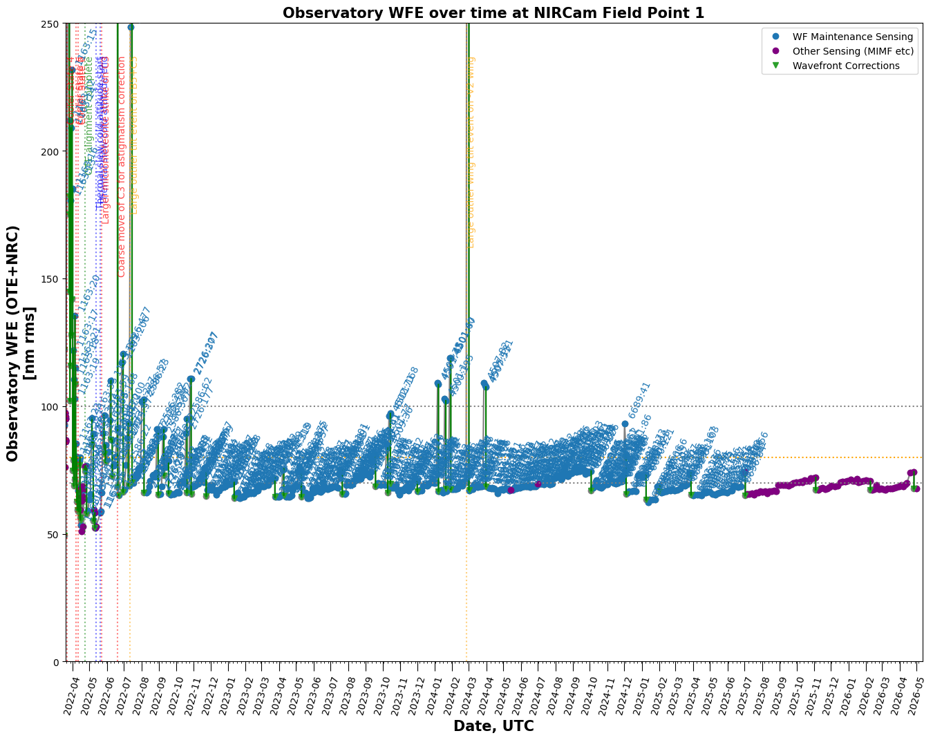
Plot over a time range#

start_date = datetime.datetime.fromisoformat('2022-11-22')
end_date = datetime.datetime.fromisoformat('2022-12-01')
stpsf.trending.wavefront_time_series_plot(opdtable, start_date=start_date,
                                          end_date=end_date, ymax=85, ymin=60,
                                          label_visits=True, label_events=True)

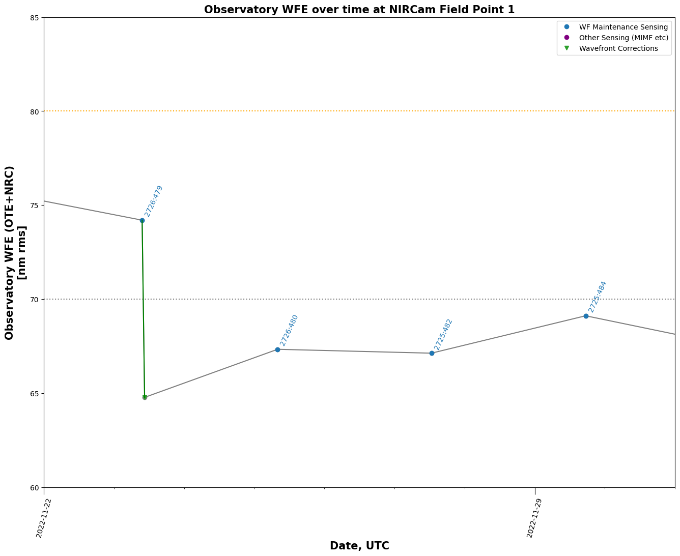
WARNING: TimeDeltaMissingUnitWarning: Numerical value without unit or explicit format passed to TimeDelta, assuming days [astropy.time.core]

../../../_images/f0cb25c35f67ef89f96d28df04f48f7443d86837add073288f6dff54f07abcda.png

# We can also plot all measured wavefront drifts over specified time periods
start_time = astropy.time.Time('2024-01-01T00:00:00')
end_time = astropy.time.Time.now()

stpsf.trending.wavefront_drift_plots(opdtable, start_time=start_time, end_time=end_time, n_per_row=10)

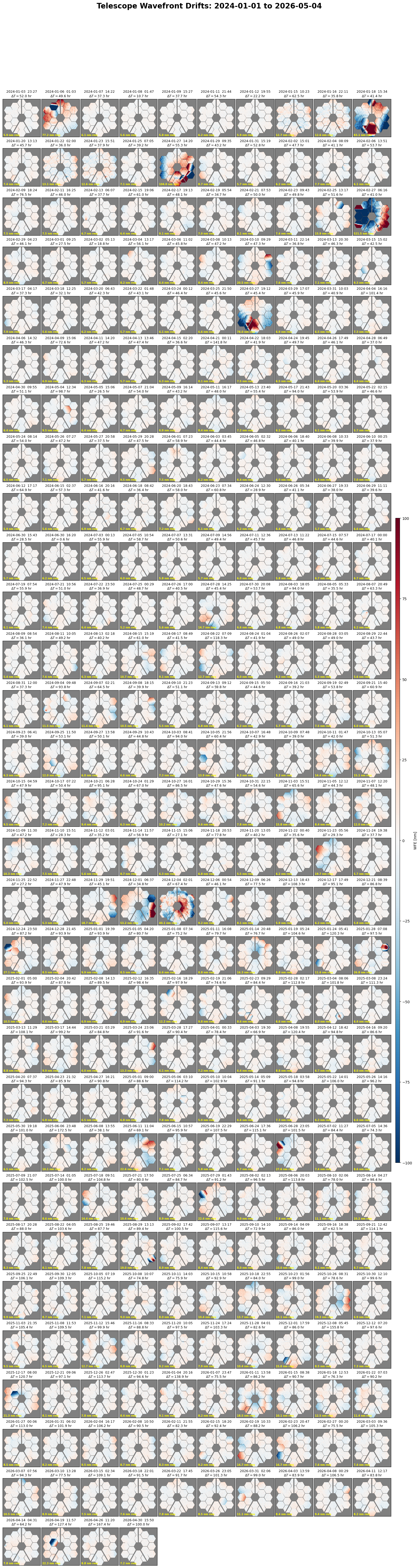
../../../_images/6dee7868365e3234cfbe15aab921f51e9e5b0d48c233c5c1c1b4e4b0efabe77f.png

# We can plot histograms of wavefront error levels over time
stpsf.trending.wfe_histogram_plot(opdtable, thresh=70, ote_only=True)

Locator attempting to generate 1040 ticks ([19144.0, ..., 20183.0]), which exceeds Locator.MAXTICKS (1000).

Locator attempting to generate 1040 ticks ([19144.0, ..., 20183.0]), which exceeds Locator.MAXTICKS (1000).

Locator attempting to generate 1040 ticks ([19144.0, ..., 20183.0]), which exceeds Locator.MAXTICKS (1000).

Locator attempting to generate 1040 ticks ([19144.0, ..., 20183.0]), which exceeds Locator.MAXTICKS (1000).

Locator attempting to generate 1040 ticks ([19144.0, ..., 20183.0]), which exceeds Locator.MAXTICKS (1000).

Locator attempting to generate 1040 ticks ([19144.0, ..., 20183.0]), which exceeds Locator.MAXTICKS (1000).

Locator attempting to generate 1040 ticks ([19144.0, ..., 20183.0]), which exceeds Locator.MAXTICKS (1000).

Locator attempting to generate 1040 ticks ([19144.0, ..., 20183.0]), which exceeds Locator.MAXTICKS (1000).

Locator attempting to generate 1040 ticks ([19144.0, ..., 20183.0]), which exceeds Locator.MAXTICKS (1000).

Locator attempting to generate 1040 ticks ([19144.0, ..., 20183.0]), which exceeds Locator.MAXTICKS (1000).

Locator attempting to generate 1040 ticks ([19144.0, ..., 20183.0]), which exceeds Locator.MAXTICKS (1000).

Locator attempting to generate 1040 ticks ([19144.0, ..., 20183.0]), which exceeds Locator.MAXTICKS (1000).

Locator attempting to generate 1040 ticks ([19144.0, ..., 20183.0]), which exceeds Locator.MAXTICKS (1000).

Locator attempting to generate 1040 ticks ([19144.0, ..., 20183.0]), which exceeds Locator.MAXTICKS (1000).

../../../_images/7822f7cfd3d392f28cf49c409660fdbd42b4879b950b8e97d3178d353c9915c5.png

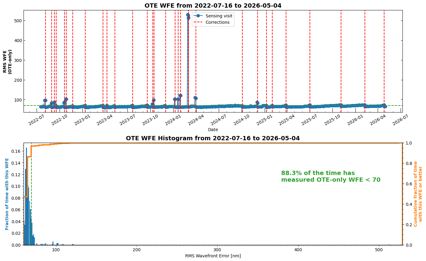
# Or select a particular time period
start_date = astropy.time.Time('2024-04-01')
end_date = astropy.time.Time.now()
stpsf.trending.wfe_histogram_plot(opdtable, start_date=start_date, thresh=70, ote_only=True)

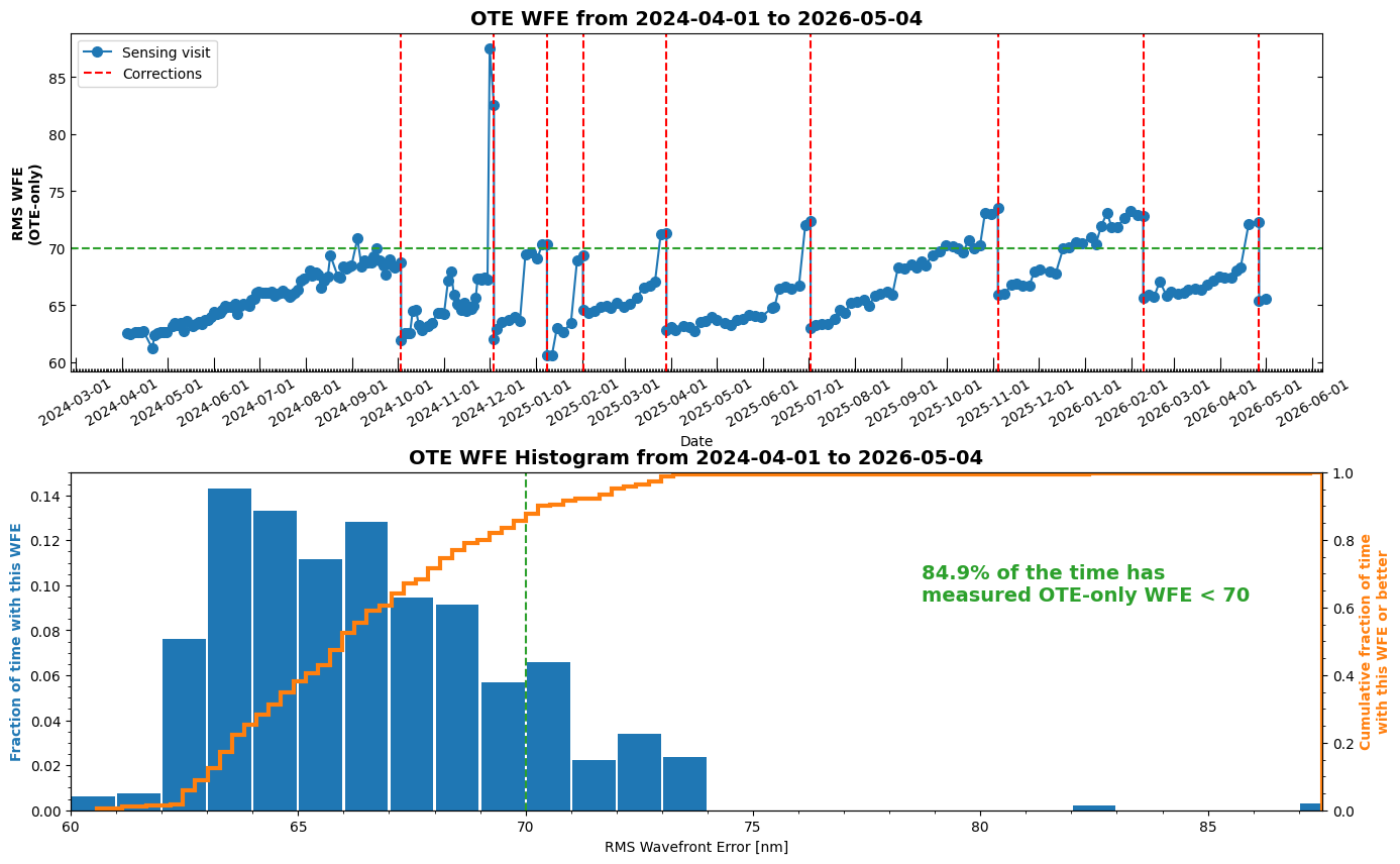
../../../_images/681301e10c35891cef332abde43f40510d559220a7e1b903ec72f450175a8bc8.png

Load and plot a Single OPD#

Inspect the OPD table above for an OPD around your observation

nrc = stpsf.NIRCam()
nrc.filter = 'F212N'
opd_fn = 'R2022120204-NRCA3_FP1-1.fits'
nrc.load_wss_opd(opd_fn, output_path=output_path)
fov_pixels = 511
psf = nrc.calc_psf(oversample=4, fov_pixels=fov_pixels)

Downloading URL https://mast.stsci.edu/api/v0.1/Download/file?uri=mast:JWST/product/R2022120204-NRCA3_FP1-1.fits to /home/runner/work/jdat_notebooks/jdat_notebooks/notebooks/cross_instrument/stpsf_examples/R2022120204-NRCA3_FP1-1.fits ...

 [Done]

Importing and format-converting OPD from /home/runner/work/jdat_notebooks/jdat_notebooks/notebooks/cross_instrument/stpsf_examples/R2022120204-NRCA3_FP1-1.fits

Backing out SI WFE and OTE field dependence at the WF sensing field point (NRCA3_FP1)

psf.info()

Filename: (No file associated with this HDUList)
No.    Name      Ver    Type      Cards   Dimensions   Format
  0  OVERSAMP      1 PrimaryHDU     104   (2044, 2044)   float64   
  1  DET_SAMP      1 ImageHDU       106   (511, 511)   float64   
  2  OVERDIST      1 ImageHDU       158   (2044, 2044)   float64   
  3  DET_DIST      1 ImageHDU       159   (511, 511)   float64   

# display the PSF and plot the encircled energy
plt.figure(figsize=(12, 6))
plt.subplot(1, 2, 1)
stpsf.display_psf(psf, colorbar_orientation='horizontal')
axis2 = plt.subplot(1, 2, 2)
stpsf.display_ee(psf, ext=1, ax=axis2)

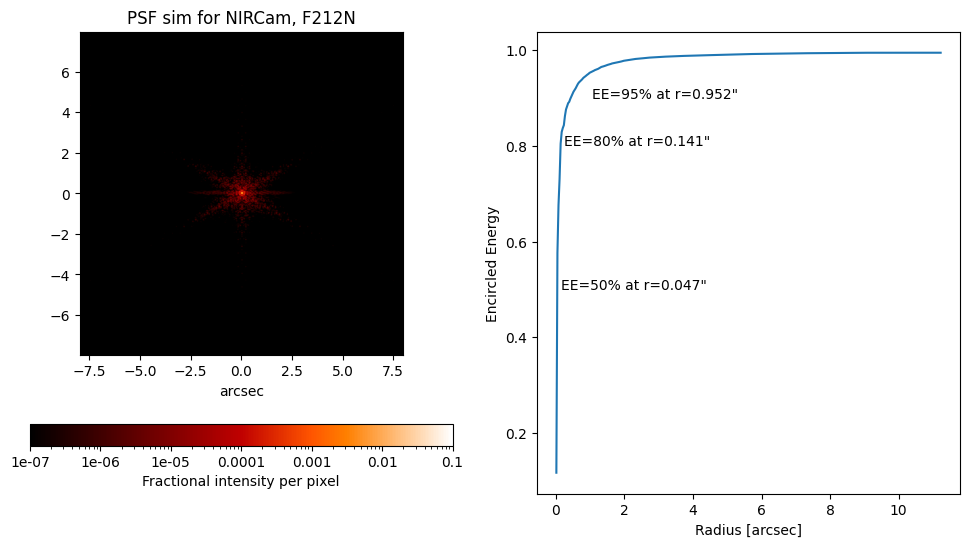
../../../_images/ed270feb8a0e9d0f9910c57e8633bc9f7c8b71b1022fc0abb3c5fe0cbd6bb1b0.png

JWST Simulated PSF Subtraction from in-flight data#

https://stpsf.readthedocs.io/en/latest/jwst_psf_subtraction.html

file = 'jw02725-o484_t097_nircam_clear-f356w-nrcalong_wfscmb-04.fits'
mast_retrieve_files(file)

Downloading URL https://mast.stsci.edu/api/v0.1/Download/file?uri=mast:JWST/product/jw02725-o484_t097_nircam_clear-f356w-nrcalong_wfscmb-04.fits to ./jw02725-o484_t097_nircam_clear-f356w-nrcalong_wfscmb-04.fits ...

 [Done]

'./jw02725-o484_t097_nircam_clear-f356w-nrcalong_wfscmb-04.fits'

# Open and inspect observation
psf = fits.open(file)
data = psf['SCI'].data
mask = (psf['DQ'].data % 2).astype('bool')
sigma_clip = SigmaClip(sigma=3.0)
bkg_estimator = MedianBackground()
# norm = simple_norm(data1, 'log',min_cut = min_cut, max_cut = max_cut)
bkg = Background2D(data, (50, 50), filter_size=(3, 3),
                   sigma_clip=sigma_clip, bkg_estimator=bkg_estimator, mask=mask)

plt.figure(figsize=(6, 6))
norm = simple_norm(data - bkg.background, 'asinh', min_percent=20, max_percent=98.99)
plt.imshow(data - bkg.background, norm=norm, origin='lower', cmap='viridis')

<matplotlib.image.AxesImage at 0x7fd9beafa6d0>

../../../_images/bcc15994f98f7dd99068bd43f39fbaebc515347e4f9492d10cce285340d9c117.png

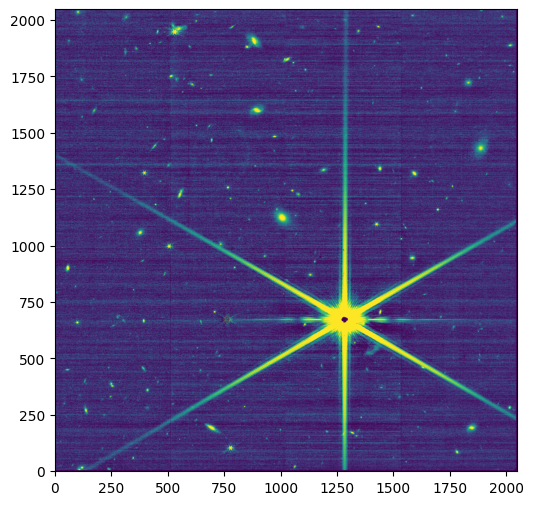
Extract a subarray around source of interest, and measure source location#

position = (550, 1950) # approximate location. This will be improved below.
size_pixels = 200

data_source = Cutout2D(data - bkg.background, position, size_pixels).data
plt.figure(figsize=(6, 6))
norm = simple_norm(data_source, 'asinh', min_percent=20, max_percent=99.6)
plt.imshow(data_source, norm=norm, origin='lower', cmap='viridis')
plt.title("Cutout around a galaxy merger and a star")

Text(0.5, 1.0, 'Cutout around a galaxy merger and a star')

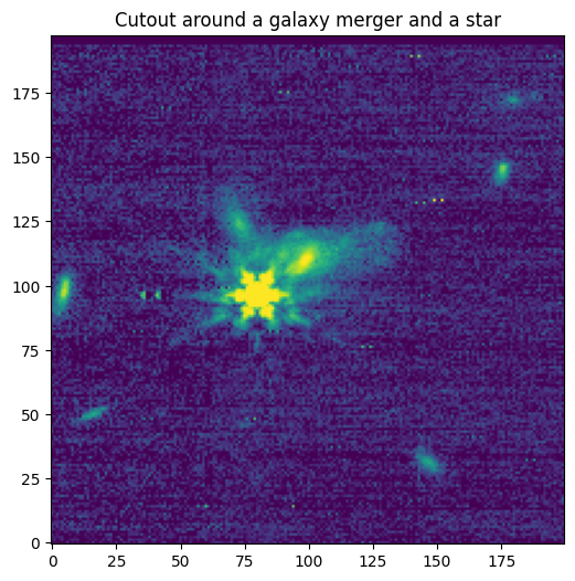
../../../_images/dca52e29af82f5d732b85416e1f2f3648359ad6d4804c10c35e586e25266d64d.png

Find the source#

starfind = IRAFStarFinder(fwhm=3.0, threshold=100. * bkg.background_median)
sources = starfind(data_source)
plt.figure(figsize=(6, 6))
plt.imshow(data_source, norm=norm, origin='lower', cmap='viridis')
plt.title("Cutout around a galaxy merger and a star")
plt.scatter(sources['xcentroid'], sources['ycentroid'], color='red', marker='x')

<matplotlib.collections.PathCollection at 0x7fd96ff21f90>

../../../_images/239a15d3195fba1a0bc2831a098ee644783c953ae92d4e3b995b94b70203f725.png

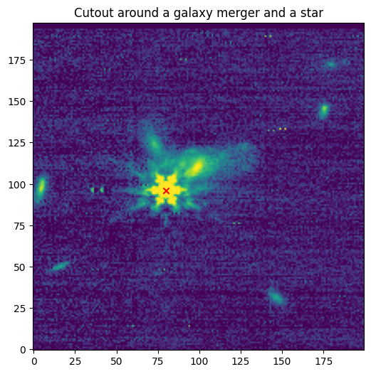
# Let's re-center the image 
positions_original = Cutout2D(data - bkg.background, position, size_pixels).to_original_position((sources['xcentroid'], sources['ycentroid']))
position = (positions_original[0].value[0], positions_original[1].value[0])
size = 200
data_source = Cutout2D(data - bkg.background, position, size_pixels).data

plt.figure(figsize=(6, 6))
norm = simple_norm(data_source, 'asinh', min_percent=20, max_percent=99.6)
plt.imshow(data_source, norm=norm, origin='lower', cmap='viridis')
plt.title("Cutout centered on the star")
print(position)

(np.float64(530.0254159648279), np.float64(1946.0672610922786))

../../../_images/9e966c604bd139749ea57a743eec8ed816016503d71258ce10cbbd7952aa15d8.png

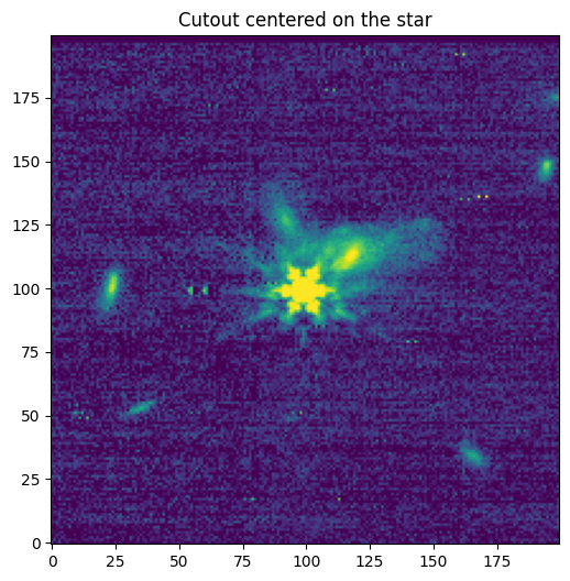
Use previous function to set up our simulation#

inst = stpsf.setup_sim_to_match_file(file)
inst.detector_position = position

single_stpsf_nrc = inst.calc_psf(fov_pixels=size_pixels)

Setting up sim to match jw02725-o484_t097_nircam_clear-f356w-nrcalong_wfscmb-04.fits
iterating query, tdelta=3.0

MAST OPD query around UTC: 2022-11-29T17:26:06.893
                        MJD: 59912.72646866898

OPD immediately preceding the given datetime:
	URI:	 mast:JWST/product/R2022112903-NRCA3_FP1-1.fits
	Date (MJD):	 59912.7265
	Delta time:	 -0.0000 days

OPD immediately following the given datetime:
	URI:	 mast:JWST/product/R2022120203-NRCA3_FP1-1.fits
	Date (MJD):	 59915.1683
	Delta time:	 2.4418 days
User requested choosing OPD time closest in time to 2022-11-29T17:26:06.893, which is R2022112903-NRCA3_FP1-1.fits, delta time -0.000 days
Downloading URL https://mast.stsci.edu/api/v0.1/Download/file?uri=mast:JWST/product/R2022112903-NRCA3_FP1-1.fits to data/stpsf-data/MAST_JWST_WSS_OPDs/R2022112903-NRCA3_FP1-1.fits ...

 [Done]

Importing and format-converting OPD from data/stpsf-data/MAST_JWST_WSS_OPDs/R2022112903-NRCA3_FP1-1.fits

Backing out SI WFE and OTE field dependence at the WF sensing field point (NRCA3_FP1)

Configured simulation instrument for:
    Instrument: NIRCam
    Filter: F356W
    Detector: NRCA5
    Apername: NRCA5_FULL
    Det. Pos.: (1024, 1024) 
    Image plane mask: None
    Pupil plane mask: None
    

single_stpsf_nrc[3].header

WARNING: VerifyWarning: Card is too long, comment will be truncated. [astropy.io.fits.card]

XTENSION= 'IMAGE   '           / Image extension                                
BITPIX  =                  -64 / array data type                                
NAXIS   =                    2 / number of array dimensions                     
NAXIS1  =                  200                                                  
NAXIS2  =                  200                                                  
PCOUNT  =                    0 / number of parameters                           
GCOUNT  =                    1 / number of groups                               
PLANE1  = 'Wavefront Intensity'                                                 
WAVELEN = 3.52998044562017E-06 / Weighted mean wavelength in meters             
DIFFLMT =   0.0976844608559387 / Diffraction limit lambda/D in arcsec           
OVERSAMP=                    1 / These data are rebinned to detector pixels     
DET_SAMP=                    4 / Oversampling factor for MFT to detector plane  
PIXELSCL=           0.06290713 / Scale in arcsec/pix (after oversampling)       
FOV     =            12.581426 / Field of view in arcsec (full array)           
NWAVES  =                   21 / Number of wavelengths used in calculation      
WAVE0   = 3.12731886916690E-06 / Wavelength 0                                   
WGHT0   = 0.029010311119741023 / Wavelength weight 0                            
WAVE1   = 3.17097412253077E-06 / Wavelength 1                                   
WGHT1   =  0.05689236899019836 / Wavelength weight 1                            
WAVE2   = 3.21462937589464E-06 / Wavelength 2                                   
WGHT2   =  0.05750257615337047 / Wavelength weight 2                            
WAVE3   = 3.25828462925851E-06 / Wavelength 3                                   
WGHT3   =  0.05665770867940551 / Wavelength weight 3                            
WAVE4   = 3.30193988262238E-06 / Wavelength 4                                   
WGHT4   =  0.05599172516198777 / Wavelength weight 4                            
WAVE5   = 3.34559513598625E-06 / Wavelength 5                                   
WGHT5   = 0.055850313012947225 / Wavelength weight 5                            
WAVE6   = 3.38925038935012E-06 / Wavelength 6                                   
WGHT6   =  0.05544478069113173 / Wavelength weight 6                            
WAVE7   = 3.43290564271399E-06 / Wavelength 7                                   
WGHT7   =  0.05465666724163407 / Wavelength weight 7                            
WAVE8   = 3.47656089607787E-06 / Wavelength 8                                   
WGHT8   =   0.0536889406582253 / Wavelength weight 8                            
WAVE9   = 3.52021614944174E-06 / Wavelength 9                                   
WGHT9   = 0.052769619836572045 / Wavelength weight 9                            
WAVE10  = 3.56387140280561E-06 / Wavelength 10                                  
WGHT10  =  0.05174556293270933 / Wavelength weight 10                           
WAVE11  = 3.60752665616948E-06 / Wavelength 11                                  
WGHT11  =    0.050926124841304 / Wavelength weight 11                           
WAVE12  = 3.65118190953335E-06 / Wavelength 12                                  
WGHT12  =  0.05008430229370746 / Wavelength weight 12                           
WAVE13  = 3.69483716289722E-06 / Wavelength 13                                  
WGHT13  =  0.04911627277824833 / Wavelength weight 13                           
WAVE14  = 3.73849241626109E-06 / Wavelength 14                                  
WGHT14  = 0.048066127719162625 / Wavelength weight 14                           
WAVE15  = 3.78214766962496E-06 / Wavelength 15                                  
WGHT15  =  0.04674715249735926 / Wavelength weight 15                           
WAVE16  = 3.82580292298883E-06 / Wavelength 16                                  
WGHT16  =   0.0454832673914629 / Wavelength weight 16                           
WAVE17  = 3.86945817635270E-06 / Wavelength 17                                  
WGHT17  = 0.044181453325114764 / Wavelength weight 17                           
WAVE18  = 3.91311342971657E-06 / Wavelength 18                                  
WGHT18  =   0.0413649282857484 / Wavelength weight 18                           
WAVE19  = 3.95676868308044E-06 / Wavelength 19                                  
WGHT19  =  0.03220514808749848 / Wavelength weight 19                           
WAVE20  = 4.00042393644431E-06 / Wavelength 20                                  
WGHT20  = 0.011614648302470809 / Wavelength weight 20                           
FFTTYPE = 'numpy.fft'          / Algorithm for FFTs: numpy or fftw              
NORMALIZ= 'first   '           / PSF normalization method                       
JITRTYPE= 'Gaussian convolution' / Type of jitter applied                       
JITRSIGM=               0.0008 / Gaussian sigma for jitter, per axis [arcsec]   
JITRSTRL=                  1.0 / Strehl reduction from jitter                   
PUPILINT= 'jwst_pupil_RevW_npix1024.fits.gz' / Pupil aperture intensity source  
PUPILOPD= 'OPD from supplied FITS HDUlist object' / Pupil OPD source            
OPD_FILE= 'R2022112903-NRCA3_FP1-1.fits' / Pupil OPD file name                  
OPDSLICE=                    0 / Pupil OPD slice number, if file is a datacube  
INSTRUME= 'NIRCam  '           / Instrument                                     
FILTER  = 'F356W   '           / Filter name                                    
EXTNAME = 'DET_DIST'           / This extension is oversampled.                 
DATE    = '2025-02-19T14:20:33' / Date of calculation                           
AUTHOR  = 'runner@fv-az1934-680' / username@host for calculation                
VERSION = '2.0.0   '           / STPSF software version                         
DATAVERS= '2.0.0   '           / STPSF reference data files version             
DET_NAME= 'NRCA5   '           / Name of detector on this instrument            
DET_X   =                530.5 / Detector X pixel position of array center      
DET_Y   =               1946.5 / Detector Y pixel position of array center      
DET_V2  =   1.9445793009682408 / [arcmin] Det. pos. in telescope V2,V3 coord sys
DET_V3  =   -7.259916804742389 / [arcmin] Det. pos. in telescope V2,V3 coord sys
TEL_WFE =    64.31211781548208 / [nm] Telescope pupil RMS wavefront error       
OTETHMDL= 'BOL     '           / OTE Thermal slew model case                    
OTETHSTA=                  0.0 / OTE Starting pitch angle for thermal slew model
OTETHEND=                  0.0 / OTE Ending pitch angle for thermal slew model  
OTETHRDT=                  0.0 / OTE Thermal slew model delta time after slew   
OTETHRWF=                  0.0 / OTE WFE amplitude from 'thermal slew' term     
OTEFRLWF=                  0.0 / OTE WFE amplitude from 'frill tension' term    
OTEIECWF=                  0.0 / OTE WFE amplitude from 'IEC thermal cycling' te
SI_WFE  =    71.92925624358796 / [nm] instrument pupil RMS wavefront error      
SIWFETYP= 'Extrapolated'       / SI WFE was extrapolated outside available meas.
SIWFEFPT= 'ISIM42  '           / Closest ISIM CV3 WFE meas. field point         
SIZERN1 = -1.0697917988307E-08 / [m] SI WFE coeff for Zernike term 1            
SIZERN2 = 3.08048159443971E-10 / [m] SI WFE coeff for Zernike term 2            
SIZERN3 = -1.9196041984348E-09 / [m] SI WFE coeff for Zernike term 3            
SIZERN4 = -8.1173126758238E-08 / [m] SI WFE coeff for Zernike term 4            
SIZERN5 = 1.51797969643943E-08 / [m] SI WFE coeff for Zernike term 5            
SIZERN6 = 4.32636655822125E-09 / [m] SI WFE coeff for Zernike term 6            
SIZERN7 = -8.0281498018401E-09 / [m] SI WFE coeff for Zernike term 7            
SIZERN8 = -1.5951952117892E-10 / [m] SI WFE coeff for Zernike term 8            
SIZERN9 = -1.9417997569617E-09 / [m] SI WFE coeff for Zernike term 9            
SIZERN10= 1.16285054335882E-09 / [m] SI WFE coeff for Zernike term 10           
SIZERN11= -1.1748250980632E-09 / [m] SI WFE coeff for Zernike term 11           
SIZERN12= -1.4078671907797E-09 / [m] SI WFE coeff for Zernike term 12           
SIZERN13= -6.6810299931733E-09 / [m] SI WFE coeff for Zernike term 13           
SIZERN14=  3.7853868843729E-09 / [m] SI WFE coeff for Zernike term 14           
SIZERN15= -1.4415140518215E-09 / [m] SI WFE coeff for Zernike term 15           
SIZERN16= -3.9703513237096E-09 / [m] SI WFE coeff for Zernike term 16           
SIZERN17= 1.31563560122644E-09 / [m] SI WFE coeff for Zernike term 17           
SIZERN18= 3.77897113698746E-10 / [m] SI WFE coeff for Zernike term 18           
SIZERN19= -1.8404320671331E-09 / [m] SI WFE coeff for Zernike term 19           
SIZERN20= -3.1559659796023E-09 / [m] SI WFE coeff for Zernike term 20           
SIZERN21= 9.70396713584626E-11 / [m] SI WFE coeff for Zernike term 21           
SIZERN22= -4.1669897552317E-09 / [m] SI WFE coeff for Zernike term 22           
SIZERN23= 1.75844652958335E-09 / [m] SI WFE coeff for Zernike term 23           
SIZERN24= 1.56437696827783E-09 / [m] SI WFE coeff for Zernike term 24           
SIZERN25= 1.98457418229480E-09 / [m] SI WFE coeff for Zernike term 25           
SIZERN26= 3.41706025271797E-10 / [m] SI WFE coeff for Zernike term 26           
SIZERN27= 1.00589037061746E-09 / [m] SI WFE coeff for Zernike term 27           
SIZERN28= 8.04885292119649E-09 / [m] SI WFE coeff for Zernike term 28           
SIZERN29= 2.44073543618285E-09 / [m] SI WFE coeff for Zernike term 29           
SIZERN30= -1.1286841969615E-09 / [m] SI WFE coeff for Zernike term 30           
SIZERN31= -2.3313034957157E-10 / [m] SI WFE coeff for Zernike term 31           
SIZERN32= 3.80384668407082E-09 / [m] SI WFE coeff for Zernike term 32           
SIZERN33= 2.87255591936445E-11 / [m] SI WFE coeff for Zernike term 33           
SIZERN34= 1.39286599091967E-09 / [m] SI WFE coeff for Zernike term 34           
SIZERN35= 1.22687031149893E-09 / [m] SI WFE coeff for Zernike term 35           
APERNAME= 'NRCA5_FULL'         / SIAF aperture name                             
MODULE  = 'A       '           / NIRCam module: A or B                          
CHANNEL = 'Long    '           / NIRCam channel: long or short                  
PILIN   = 'False   '           / Pupil imaging lens in optical path: T/F        
ROTATION=          -0.06338311 / PSF rotated to match detector rotation         
DISTORT = 'True    '           / SIAF distortion coefficients applied           
SIAF_VER= 'PRDOPSSOC-068'      / SIAF PRD version used                          
COEF_X00=                  0.0 / SIAF distortion coefficient for Idl2SciX00     
COEF_X10=         15.935064289 / SIAF distortion coefficient for Idl2SciX10     
COEF_X11=     0.00062662311666 / SIAF distortion coefficient for Idl2SciX11     
COEF_X20=     -0.0004866509075 / SIAF distortion coefficient for Idl2SciX20     
COEF_X21=      0.0029284279113 / SIAF distortion coefficient for Idl2SciX21     
COEF_X22=     0.00038194617433 / SIAF distortion coefficient for Idl2SciX22     
COEF_X30=     -6.765142999E-06 / SIAF distortion coefficient for Idl2SciX30     
COEF_X31=    -2.5133479064E-08 / SIAF distortion coefficient for Idl2SciX31     
COEF_X32=    -5.9888336301E-06 / SIAF distortion coefficient for Idl2SciX32     
COEF_X33=     9.6468885579E-08 / SIAF distortion coefficient for Idl2SciX33     
COEF_X40=     4.7744230522E-09 / SIAF distortion coefficient for Idl2SciX40     
COEF_X41=    -2.0517544492E-09 / SIAF distortion coefficient for Idl2SciX41     
COEF_X42=     1.3815714874E-09 / SIAF distortion coefficient for Idl2SciX42     
COEF_X43=     -2.426584853E-09 / SIAF distortion coefficient for Idl2SciX43     
COEF_X44=     1.2928805585E-09 / SIAF distortion coefficient for Idl2SciX44     
COEF_X50=     1.3344738859E-11 / SIAF distortion coefficient for Idl2SciX50     
COEF_X51=    -5.3342857046E-11 / SIAF distortion coefficient for Idl2SciX51     
COEF_X52=    -1.0440706849E-10 / SIAF distortion coefficient for Idl2SciX52     
COEF_X53=    -1.7536898874E-11 / SIAF distortion coefficient for Idl2SciX53     
COEF_X54=    -3.4500183346E-11 / SIAF distortion coefficient for Idl2SciX54     
COEF_X55=     1.5806704408E-11 / SIAF distortion coefficient for Idl2SciX55     
COEF_Y00=                  0.0 / SIAF distortion coefficient for Idl2SciY00     
COEF_Y10=       0.023739771631 / SIAF distortion coefficient for Idl2SciY10     
COEF_Y11=         15.858052334 / SIAF distortion coefficient for Idl2SciY11     
COEF_Y20=     -0.0012404007583 / SIAF distortion coefficient for Idl2SciY20     
COEF_Y21=    -0.00089790574444 / SIAF distortion coefficient for Idl2SciY21     
COEF_Y22=      0.0017034211874 / SIAF distortion coefficient for Idl2SciY22     
COEF_Y30=     2.0629748211E-07 / SIAF distortion coefficient for Idl2SciY30     
COEF_Y31=    -7.0626833341E-06 / SIAF distortion coefficient for Idl2SciY31     
COEF_Y32=    -3.4856432882E-07 / SIAF distortion coefficient for Idl2SciY32     
COEF_Y33=    -6.1165886835E-06 / SIAF distortion coefficient for Idl2SciY33     
COEF_Y40=    -3.6220865015E-09 / SIAF distortion coefficient for Idl2SciY40     
COEF_Y41=     1.4877764101E-09 / SIAF distortion coefficient for Idl2SciY41     
COEF_Y42=    -3.5926010043E-09 / SIAF distortion coefficient for Idl2SciY42     
COEF_Y43=     5.2665557003E-10 / SIAF distortion coefficient for Idl2SciY43     
COEF_Y44=    -3.8007690059E-09 / SIAF distortion coefficient for Idl2SciY44     
COEF_Y50=    -1.8738092393E-11 / SIAF distortion coefficient for Idl2SciY50     
COEF_Y51=    -2.7459579135E-11 / SIAF distortion coefficient for Idl2SciY51     
COEF_Y52=     1.7468257099E-11 / SIAF distortion coefficient for Idl2SciY52     
COEF_Y53=    -8.7857813876E-11 / SIAF distortion coefficient for Idl2SciY53     
COEF_Y54=    -1.6157416544E-12 / SIAF distortion coefficient for Idl2SciY54     
COEF_Y55=    -5.0913836989E-11 / SIAF distortion coefficient for Idl2SciY55     
CHDFTYPE= 'gaussian'           / Type of detector charge diffusion model        
CHDFSIGM=                0.018 / [arcsec] Gaussian sigma for charge diff model  
CALCSAMP=                    4 / This much oversampling used in calculation     
IPCINST = 'NIRCam  '           / Interpixel capacitance (IPC)                   
IPCTYPA = '485     '           / NRC SCA num used for IPC and PPC model         
IPCFILE = 'KERNEL_IPC_CUBE.fits' / IPC model source file                        
PPCFILE = 'KERNEL_PPC_CUBE.fits' / PPC model source file                        
HISTORY Created wavefront: wavelength=3.127e-06 m, diam=6.603 m                 
HISTORY  using array size (1024, 1024)                                          
HISTORY   Multiplied WF by phasor for Pupil plane: JWST Entrance Pupil          
HISTORY   Propagating wavefront to Coordinate Inversion in y axis.              
HISTORY Inverted axis direction for Y axes                                      
HISTORY   Multiplied WF by phasor for Pupil plane: NIRCamLWA internal WFE at V2V
HISTORY 3=(1.94,-7.26)', near ISIM42                                            
HISTORY   Propagating wavefront to Detector plane: NIRCam detector (200x200 pixe
HISTORY ls, 0.063 arcsec / pix).                                                
HISTORY     Propagating w/ MFT: 0.0157 arcsec / pix     fov=128.797 lam/D    npi
HISTORY x=800                                                                   
HISTORY Calculation completed in 5.300 seconds                                  
HISTORY Created by POPPY version                                                
HISTORY Applied detector charge diffusion model.                                
HISTORY Applied detector interpixel capacitance (IPC) model                     

Use photutils to create our model PSF#

We’ll use photutils to fit and subtract the PSF from the data. First, we take the output simulated PSF and convert it into a photutils fittable model:

stpsf_model = photutils.psf.FittableImageModel(single_stpsf_nrc['DET_DIST'].data, normalize=True, oversampling=1)

WARNING: AstropyDeprecationWarning: The FittableImageModel class is deprecated and may be removed in a future version.
        Use `ImagePSF` instead. [warnings]

fit_shape = (5, 5)
psfphot = PSFPhotometry(stpsf_model, fit_shape,
                        finder=starfind, aperture_radius=4)

# fit model PSF to background subtracted data
phot = psfphot(data_source)

Check the location of the source to be subtracted#

print(phot) # single source

 id group_id group_size ...         qfit                 cfit         flags
--- -------- ---------- ... ------------------- --------------------- -----
  1        1          1 ... 0.06846369463654885 -0.007573722037113907     0

Subtract PSF and create residual image#

residual = psfphot.make_residual_image(data_source, psf_shape=(size_pixels, size_pixels))

plt.figure(figsize=(14, 16))

plt.subplot(1, 2, 1)
plt.imshow(data_source, norm=norm, origin='lower', cmap='viridis')
plt.title('Original - zoom')

plt.subplot(1, 2, 2)
plt.imshow(residual, norm=norm, origin='lower', cmap='viridis')
plt.title('Clean - PSFPhotometry zoom')

Text(0.5, 1.0, 'Clean - PSFPhotometry zoom')

../../../_images/b82e82883e72d7e281719dec80534cc8396c1ff4f678e2e05f7e12a1479d1a91.png

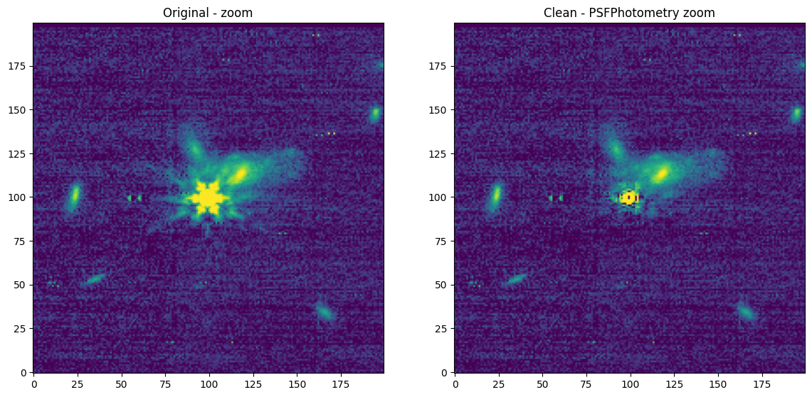
PSF properties and differences#

pixelscale = nrc.pixelscale 
ee_pixel_radius = 2.5
ee_arcsec_radius = ee_pixel_radius * pixelscale
ee_psf = poppy.measure_ee(single_stpsf_nrc, ext=3, normalize='total')
ee_val = ee_psf(ee_arcsec_radius)
print("ee ({}px, {:.3f}arsec)  = {:.4f}".format(ee_pixel_radius, ee_arcsec_radius, ee_val.item(0)))

ee (2.5px, 0.078arsec)  = 0.5124

def measure_fwhm(array):
    """Fit a Gaussian2D model to a PSF and return the fitted PSF
    the FWHM is x and y can be found with fitted_psf.x_fwhm, fitted_psf.y_fwhm

    Parameters
    ----------
    array : numpy.ndarray
        Array containing PSF

    Returns
    -------
    x_fwhm : float
        FWHM in x direction in units of pixels

    y_fwhm : float
        FWHM in y direction in units of pixels
        
    x_mean : float
        x centroid position in units of pixels
    
    y_mean : float
        y centroid position in units of pixels
    
    """
    yp, xp = array.shape
    y, x = np.mgrid[:yp, :xp]
    p_init = models.Gaussian2D(amplitude=array.max(), x_mean=xp * 0.5, y_mean=yp * 0.5)
    fit_p = fitting.LevMarLSQFitter()
    fitted_psf = fit_p(p_init, x, y, array)
    return fitted_psf

fitted_psf = measure_fwhm(single_stpsf_nrc["DET_SAMP"].data)
print("FWHM X-direction: {:.3f}, FWHM y-direction: {:.2f}".format(fitted_psf.x_fwhm, fitted_psf.y_fwhm))

FWHM X-direction: 1.835, FWHM y-direction: 1.88

# Note that the OPD is loaded in STPSF instrument object
# norm = ImageNormalize(stretch=LinearStretch(), vmin = 1e-9 , vmax = 1e-7)
plt.figure(figsize=[10, 10])
plt.imshow(nrc.pupilopd[0].data, origin='lower')

<matplotlib.image.AxesImage at 0x7fd971126590>

../../../_images/d00ab2ca801f8b9597e602dac9c313ed7ddad1cd13edeb990b5a615dd293dfd4.png

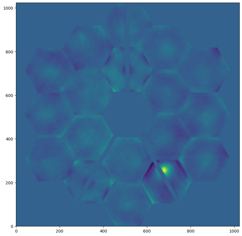
# check OPD header information
nrc.pupilopd[0].header

SIMPLE  =                    T / Written by IDL:  Fri Dec  2 22:39:16 2022      
BITPIX  =                  -64 / Number of bits per data pixel                  
NAXIS   =                    2 / Number of data axes                            
NAXIS1  =                 1024                                                  
NAXIS2  =                 1024                                                  
EXTEND  =                    T / FITS data may contain extensions               
DATE    = '2022-12-02'         / Creation UTC (CCCC-MM-DD) date of FITS header  
COMMENT FITS (Flexible Image Transport System) format is defined in 'Astronomy  
COMMENT and Astrophysics', volume 376, page 359; bibcode 2001A&A...376..359H    
FILECONT= 'Analysis output products' /                                          
TSTAMP  = '2022-12-02T22:39:16' /                                               
DATE-OBS= '2022-12-02'         /                                                
TIME-OBS= '04:02:21.595'       /                                                
OBS_ID  = 'V02724347001P0000000003104' /                                        
OP_TYPE = 'WAVEFRONT_MAINTENANCE' /                                             
MODE    = 'AUTOMATIC'          /                                                
OPER    = 'TRUE    '           /                                                
CORR_ID = 'R2022120204'        /                                                
GROUP_ID=                    1 /                                                
GRP_CNT =                    2 /                                                
INSTRUME= 'NIRCam-A'           /                                                
DETECTOR= 'NRCA3   '           /                                                
APERNAME= 'NRCA3_FP1'          /                                                
FPX     =             -1.16891 /                                                
FPY     =            -0.767005 /                                                
BUNIT   = 'm       '                                                            
PUPLDIAM=             6.603464                                                  
PUPLSCAL=      0.0064486953125                                                  
CONTENTS= 'Estimated OTE WFE from Wavefront Sensing Measurements'               
HISTORY OPD file retrieved from MAST for use by STPSF.                          
HISTORY Converting input for use with STPSF:                                    
HISTORY   Input file is: /home/runner/work/jdat_notebooks/jdat_notebooks/noteboo
HISTORY ks/cross_instrument/stpsf_examples/R2022120204-NRCA3_FP1-1.fits         
HISTORY   Need to rescale from 256x256 to 1024x1024 pixels.                     
HISTORY   Dilated OPD values to fill adjacent invalid pixels (i.e. fill in gaps)
HISTORY   Interpolated array to 1024x1024 pixels across                         
HISTORY   Converted units from microns to meters                                
HISTORY Estimating SI WFE at sensing field point NRCA3_FP1.                     
HISTORY   See FITS extension SENSING_SI_WFE for the SI WFE model used.          
HISTORY   Subtracted SI WFE to estimate OTE-only global WFE.                    
HISTORY Estimating OTE field dependence term at NRCA3_FP1.                      
HISTORY   Selected instrument field point is at V2,V3 = [ 1.1595149  -8.59714411
HISTORY ] arcmin.                                                               
HISTORY   See FITS extension SENSING_OTE_FD_WFE for the WFE model used.         
HISTORY   Subtracted OTE field dependence to estimate OTE global WFE.           

# Let's calculate the difference between two different times
# We can use the same instrument setup from before
opd_fn = 'R2022120404-NRCA3_FP1-1.fits'
inst.load_wss_opd(opd_fn)
psf2 = inst.calc_psf(fov_pixels=size_pixels)

Found OPD file previously downloaded: R2022120404-NRCA3_FP1-1.fits
Importing and format-converting OPD from data/stpsf-data/MAST_JWST_WSS_OPDs/R2022120404-NRCA3_FP1-1.fits
Backing out SI WFE and OTE field dependence at the WF sensing field point (NRCA3_FP1)

pixelscale = nrc.pixelscale
ee_pixel_radius = 2.5
ee_arcsec_radius = ee_pixel_radius * pixelscale
ee_psf = poppy.measure_ee(psf2, ext=1, normalize='total')
ee_val = ee_psf(ee_arcsec_radius)
print("ee ({}px, {:.3f}arsec)  = {:.4f}".format(ee_pixel_radius, ee_arcsec_radius, ee_val.item(0)))

ee (2.5px, 0.078arsec)  = 0.5545

stpsf.display_psf_difference(single_stpsf_nrc, psf2, imagecrop=2, title='Difference between two OPDs', cmap='gist_heat')

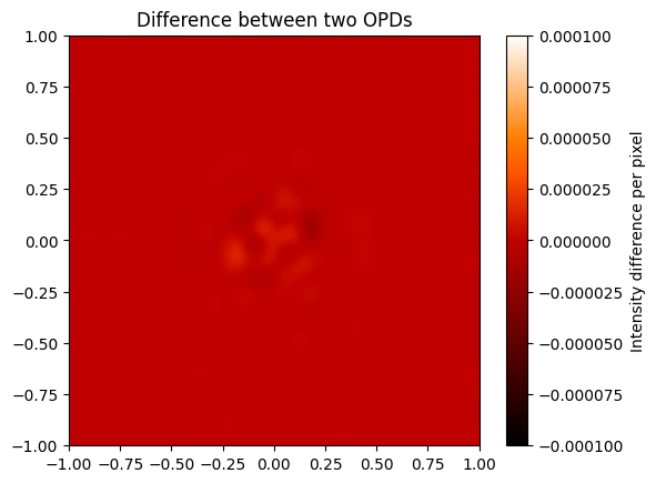
../../../_images/cdcd2dad780c2b0d0a44a88ecf477b853612de93c3a2f3b16d51f20c3a694766.png

def miri_psfs_for_ee():
    miri = stpsf.MIRI()

    # opd_fn = 'R2022120404-NRCA3_FP1-1.fits'
    # miri.load_wss_opd(opd_fn, output_path = output_path)
    miri.load_wss_opd_by_date('2022-07-12T00:00:00', plot=True, output_path=output_path)

    for wave in [5.0, 7.5, 10, 14]:
        fov = 18

        outname = "PSF_MIRI_%.1fum_wfed.fits" % (wave)
        psf = miri.calc_psf(outname, monochromatic=wave * 1e-6,
                            oversample=4, fov_arcsec=fov, display=True)
    return psf


def plot_ee_curves():
    plt.clf()
    for iw, wave in enumerate([5.0, 7.5, 10, 14]):

        ees60 = []
        ees51 = []
        ax = plt.subplot(2, 2, iw+1)
       
        name = "PSF_MIRI_%.1fum_wfed.fits" % (wave)
        stpsf.display_ee(name, ax=ax, mark_levels=False)

        eefn = stpsf.measure_ee(name)
        ees60.append(eefn(0.60))
        ees51.append(eefn(0.51))

        ax.text(1, 0.6, 'Mean EE inside 0.60": %.3f' % np.asarray(ees60).mean())
        ax.text(1, 0.5, 'Mean EE inside 0.51": %.3f' % np.asarray(ees51).mean())

        ax.set_title(f"Wavelength = {wave:.1f} $\\mu$m")

        ax.axvline(0.6, ls=":", color='k')
        ax.axvline(0.51, ls=":", color='k')

    plt.tight_layout()   

miri_psfs_for_ee()

iterating query, tdelta=3.0

MAST OPD query around UTC: 2022-07-12T00:00:00.000
                        MJD: 59772.0

OPD immediately preceding the given datetime:
	URI:	 mast:JWST/product/O2022071001-NRCA3_FP1-0.fits
	Date (MJD):	 59770.4830
	Delta time:	 -1.5170 days

OPD immediately following the given datetime:
	URI:	 mast:JWST/product/R2022071302-NRCA3_FP1-1.fits
	Date (MJD):	 59772.6632
	Delta time:	 0.6632 days
User requested choosing OPD time closest in time to 2022-07-12T00:00:00.000, which is R2022071302-NRCA3_FP1-1.fits, delta time 0.663 days

Downloading URL https://mast.stsci.edu/api/v0.1/Download/file?uri=mast:JWST/product/R2022071302-NRCA3_FP1-1.fits to /home/runner/work/jdat_notebooks/jdat_notebooks/notebooks/cross_instrument/stpsf_examples/R2022071302-NRCA3_FP1-1.fits ...

 [Done]

Importing and format-converting OPD from /home/runner/work/jdat_notebooks/jdat_notebooks/notebooks/cross_instrument/stpsf_examples/R2022071302-NRCA3_FP1-1.fits

Backing out SI WFE and OTE field dependence at the WF sensing field point (NRCA3_FP1)

WARNING: VerifyWarning: Card is too long, comment will be truncated. [astropy.io.fits.card]

WARNING: VerifyWarning: Card is too long, comment will be truncated. [astropy.io.fits.card]

WARNING: VerifyWarning: Card is too long, comment will be truncated. [astropy.io.fits.card]

WARNING: VerifyWarning: Card is too long, comment will be truncated. [astropy.io.fits.card]

[<astropy.io.fits.hdu.image.PrimaryHDU object at 0x7fd953be9950>, <astropy.io.fits.hdu.image.ImageHDU object at 0x7fd953baf8d0>, <astropy.io.fits.hdu.image.ImageHDU object at 0x7fd953fa1d50>, <astropy.io.fits.hdu.image.ImageHDU object at 0x7fd9583eafd0>]

../../../_images/5d2915f24aedd5f33e2f46e43ba0183991c35e0fb836aefa7ba7082b5d1b8f4a.png

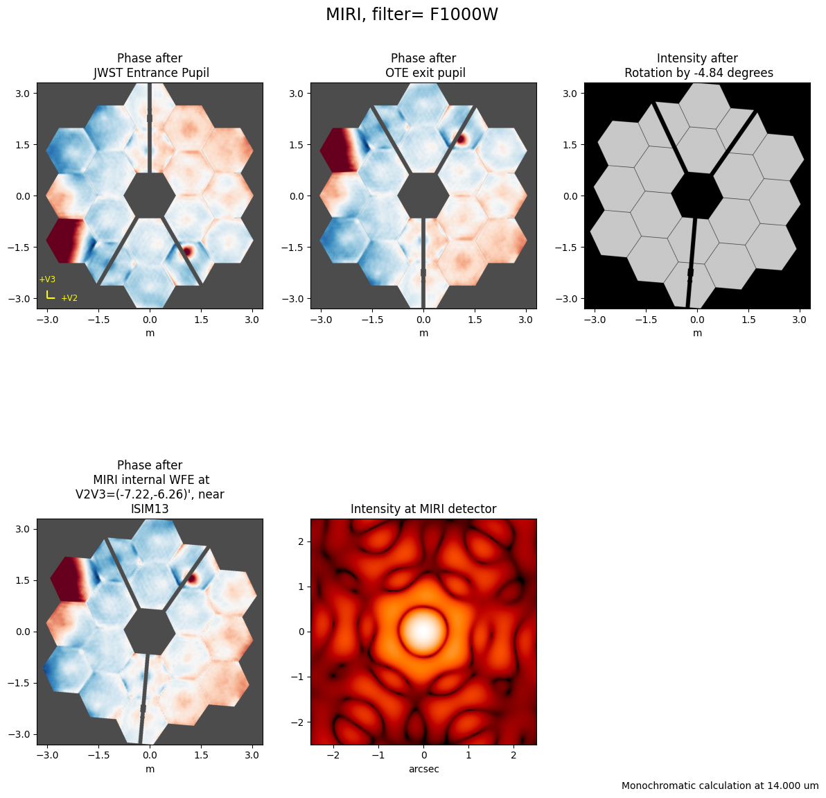
plot_ee_curves()

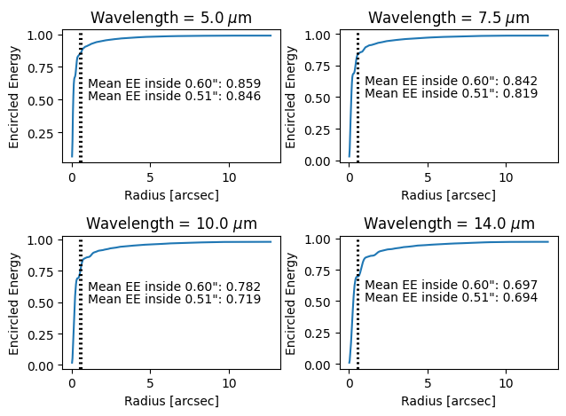
../../../_images/0383ae702af075e574ea498504086864c64993c67be084580a8bbd7dc9685da7.png

nsp = stpsf.NIRSpec()
# or you can specify a full path name.
# please make an output PSF with its center
# aligned to the center of a single pixel
nsp.options['parity'] = 'odd'

opd_fn = 'R2022120404-NRCA3_FP1-1.fits'
nsp.load_wss_opd(opd_fn, output_path=output_path)
    
waves = np.linspace(0.8, 5, 50) * 1e-6 # iterate over wavelengths in meters

for iw, wavelength in enumerate(waves):
    psffile = 'psf_NIRSPec_mono_%.1fum_opd1.fits' % (wavelength * 1e6)
    psf = nsp.calc_psf(fov_arcsec=3, oversample=4, 
                       monochromatic=wavelength, display=False,
                       outfile=psffile)
    ax = plt.subplot(8, 8, iw + 1)
    stpsf.display_psf(psffile, ext='DET_SAMP', colorbar=False, imagecrop=8)
    ax.set_title('')
    ax.xaxis.set_visible(False)
    ax.yaxis.set_visible(False)
    ax.text(-3.5, 0, '{0:.1f}'.format(wavelength * 1e6))

Downloading URL https://mast.stsci.edu/api/v0.1/Download/file?uri=mast:JWST/product/R2022120404-NRCA3_FP1-1.fits to /home/runner/work/jdat_notebooks/jdat_notebooks/notebooks/cross_instrument/stpsf_examples/R2022120404-NRCA3_FP1-1.fits ...

 [Done]

Importing and format-converting OPD from /home/runner/work/jdat_notebooks/jdat_notebooks/notebooks/cross_instrument/stpsf_examples/R2022120404-NRCA3_FP1-1.fits
Backing out SI WFE and OTE field dependence at the WF sensing field point (NRCA3_FP1)

WARNING: VerifyWarning: Card is too long, comment will be truncated. [astropy.io.fits.card]

WARNING: VerifyWarning: Card is too long, comment will be truncated. [astropy.io.fits.card]

WARNING: VerifyWarning: Card is too long, comment will be truncated. [astropy.io.fits.card]

WARNING: VerifyWarning: Card is too long, comment will be truncated. [astropy.io.fits.card]

WARNING: VerifyWarning: Card is too long, comment will be truncated. [astropy.io.fits.card]

WARNING: VerifyWarning: Card is too long, comment will be truncated. [astropy.io.fits.card]

WARNING: VerifyWarning: Card is too long, comment will be truncated. [astropy.io.fits.card]

WARNING: VerifyWarning: Card is too long, comment will be truncated. [astropy.io.fits.card]

WARNING: VerifyWarning: Card is too long, comment will be truncated. [astropy.io.fits.card]

WARNING: VerifyWarning: Card is too long, comment will be truncated. [astropy.io.fits.card]

WARNING: VerifyWarning: Card is too long, comment will be truncated. [astropy.io.fits.card]

WARNING: VerifyWarning: Card is too long, comment will be truncated. [astropy.io.fits.card]

WARNING: VerifyWarning: Card is too long, comment will be truncated. [astropy.io.fits.card]

WARNING: VerifyWarning: Card is too long, comment will be truncated. [astropy.io.fits.card]

WARNING: VerifyWarning: Card is too long, comment will be truncated. [astropy.io.fits.card]

WARNING: VerifyWarning: Card is too long, comment will be truncated. [astropy.io.fits.card]

WARNING: VerifyWarning: Card is too long, comment will be truncated. [astropy.io.fits.card]

WARNING: VerifyWarning: Card is too long, comment will be truncated. [astropy.io.fits.card]

WARNING: VerifyWarning: Card is too long, comment will be truncated. [astropy.io.fits.card]

WARNING: VerifyWarning: Card is too long, comment will be truncated. [astropy.io.fits.card]

WARNING: VerifyWarning: Card is too long, comment will be truncated. [astropy.io.fits.card]

WARNING: VerifyWarning: Card is too long, comment will be truncated. [astropy.io.fits.card]

WARNING: VerifyWarning: Card is too long, comment will be truncated. [astropy.io.fits.card]

WARNING: VerifyWarning: Card is too long, comment will be truncated. [astropy.io.fits.card]

WARNING: VerifyWarning: Card is too long, comment will be truncated. [astropy.io.fits.card]

WARNING: VerifyWarning: Card is too long, comment will be truncated. [astropy.io.fits.card]

WARNING: VerifyWarning: Card is too long, comment will be truncated. [astropy.io.fits.card]

WARNING: VerifyWarning: Card is too long, comment will be truncated. [astropy.io.fits.card]

WARNING: VerifyWarning: Card is too long, comment will be truncated. [astropy.io.fits.card]

WARNING: VerifyWarning: Card is too long, comment will be truncated. [astropy.io.fits.card]

WARNING: VerifyWarning: Card is too long, comment will be truncated. [astropy.io.fits.card]

WARNING: VerifyWarning: Card is too long, comment will be truncated. [astropy.io.fits.card]

WARNING: VerifyWarning: Card is too long, comment will be truncated. [astropy.io.fits.card]

WARNING: VerifyWarning: Card is too long, comment will be truncated. [astropy.io.fits.card]

WARNING: VerifyWarning: Card is too long, comment will be truncated. [astropy.io.fits.card]

WARNING: VerifyWarning: Card is too long, comment will be truncated. [astropy.io.fits.card]

WARNING: VerifyWarning: Card is too long, comment will be truncated. [astropy.io.fits.card]

WARNING: VerifyWarning: Card is too long, comment will be truncated. [astropy.io.fits.card]

WARNING: VerifyWarning: Card is too long, comment will be truncated. [astropy.io.fits.card]

WARNING: VerifyWarning: Card is too long, comment will be truncated. [astropy.io.fits.card]

WARNING: VerifyWarning: Card is too long, comment will be truncated. [astropy.io.fits.card]

WARNING: VerifyWarning: Card is too long, comment will be truncated. [astropy.io.fits.card]

WARNING: VerifyWarning: Card is too long, comment will be truncated. [astropy.io.fits.card]

WARNING: VerifyWarning: Card is too long, comment will be truncated. [astropy.io.fits.card]

WARNING: VerifyWarning: Card is too long, comment will be truncated. [astropy.io.fits.card]

WARNING: VerifyWarning: Card is too long, comment will be truncated. [astropy.io.fits.card]

WARNING: VerifyWarning: Card is too long, comment will be truncated. [astropy.io.fits.card]

WARNING: VerifyWarning: Card is too long, comment will be truncated. [astropy.io.fits.card]

WARNING: VerifyWarning: Card is too long, comment will be truncated. [astropy.io.fits.card]

WARNING: VerifyWarning: Card is too long, comment will be truncated. [astropy.io.fits.card]

../../../_images/97d4636a578b25eb2d488b30716549b96f413967d768f721b500fca6b1294454.png

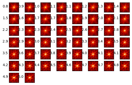
plt.figure(figsize=(8, 12))
nsp.image_mask = 'MSA all open'
nsp.display()
msapsf = nsp.calc_psf(monochromatic=2e-6, oversample=8)
stpsf.display_psf(msapsf, ext='DET_SAMP')

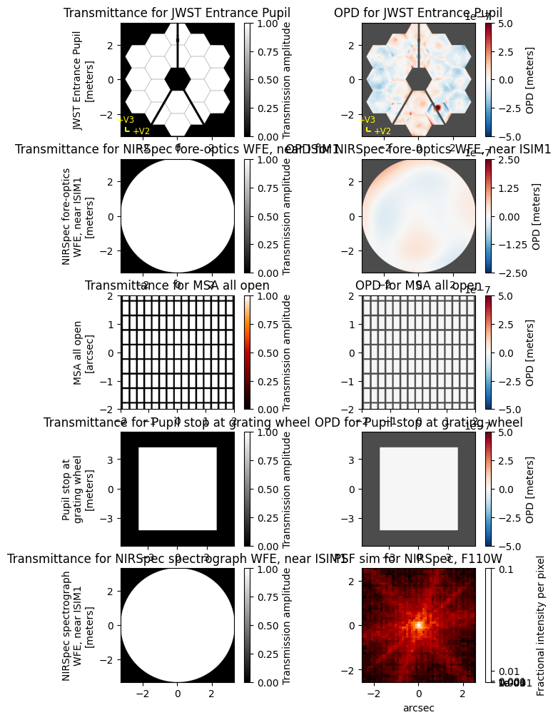
../../../_images/1b58dd05301e4091a86c5b125591adc97adddf495d0dd8d95fde659203469aed.png

miri_psfs_for_ee()

iterating query, tdelta=3.0

MAST OPD query around UTC: 2022-07-12T00:00:00.000
                        MJD: 59772.0

OPD immediately preceding the given datetime:
	URI:	 mast:JWST/product/O2022071001-NRCA3_FP1-0.fits
	Date (MJD):	 59770.4830
	Delta time:	 -1.5170 days

OPD immediately following the given datetime:
	URI:	 mast:JWST/product/R2022071302-NRCA3_FP1-1.fits
	Date (MJD):	 59772.6632
	Delta time:	 0.6632 days
User requested choosing OPD time closest in time to 2022-07-12T00:00:00.000, which is R2022071302-NRCA3_FP1-1.fits, delta time 0.663 days

Importing and format-converting OPD from /home/runner/work/jdat_notebooks/jdat_notebooks/notebooks/cross_instrument/stpsf_examples/R2022071302-NRCA3_FP1-1.fits
Backing out SI WFE and OTE field dependence at the WF sensing field point (NRCA3_FP1)

WARNING: VerifyWarning: Card is too long, comment will be truncated. [astropy.io.fits.card]

WARNING: VerifyWarning: Card is too long, comment will be truncated. [astropy.io.fits.card]

WARNING: VerifyWarning: Card is too long, comment will be truncated. [astropy.io.fits.card]

WARNING: VerifyWarning: Card is too long, comment will be truncated. [astropy.io.fits.card]

[<astropy.io.fits.hdu.image.PrimaryHDU object at 0x7fd96cffc090>, <astropy.io.fits.hdu.image.ImageHDU object at 0x7fd96dbe5890>, <astropy.io.fits.hdu.image.ImageHDU object at 0x7fd96cff3a10>, <astropy.io.fits.hdu.image.ImageHDU object at 0x7fd96ed7a410>]

plot_ee_curves()

Improved IFU sims#

miri = stpsf.MIRI()
miri.mode = 'IFU'
miri.band = '2A'
waves = miri.get_IFU_wavelengths()
cube = miri.calc_datacube_fast(waves)

/opt/hostedtoolcache/Python/3.11.11/x64/lib/python3.11/site-packages/stpsf/opds.py:1759: UserWarning: For (V2,V3) = [-8.39108833 -5.32144667] arcmin, Field point -8.254199999999999 arcmin, -2.478553333333333 arcmin not within valid region for field dependence model of OTE WFE for MIRI: -8.254199999999999 arcmin--6.21738 arcmin, -2.557224 arcmin--0.5632056 arcmin.  Clipping to closest available valid location, 0.13688833333333505 arcmin away from the requested coordinates.
  warnings.warn(warning_message)

cube.info()

Filename: (No file associated with this HDUList)
No.    Name      Ver    Type      Cards   Dimensions   Format
  0  OVERSAMP      1 PrimaryHDU    1075   (284, 284, 970)   float64   

nrs = stpsf.NIRSpec()
nrs.mode = 'IFU'
nrs.disperser = 'PRISM'
nrs.filter = 'CLEAR'
waves = nrs.get_IFU_wavelengths()
cube = nrs.calc_datacube_fast(waves)

cube.info()

Filename: (No file associated with this HDUList)
No.    Name      Ver    Type      Cards   Dimensions   Format
  0  OVERSAMP      1 PrimaryHDU    1049   (192, 192, 940)   float64   