Photometry of a JWST/NIRCam extragalactic field with Photutils

Author: Larry Bradley, Space Telescope Science Institute
Data last modified: 2025-02-27

Tutorial Overview

This tutorial will demonstrate how to use Photutils to perform multiband NIRCam photometry on an extragalactic field.

Photutils is a Python library that provides commonly-used tools and key functionality for detecting and performing photometry of astronomical sources. Tools are provided for

• background estimation

• star finding

• source detection and extraction

• aperture photometry

• PSF photometry

• image segmentation

• centroids

• radial profiles

• elliptical isophote fitting

It is a coordinated package of Astropy and integrates well with other Astropy packages, making it a powerful tool for astronomical image analysis.

Outline:

1. Load Datasets

2. Background Subtraction

3. Aperture Photometry

4. Creating a multiband segmentation-based catalog

   1. Creating a Detection Image

   2. Source Extraction via Image Segmentation

   3. Source Deblending

   4. Modifying a Segmentation Image

   5. SourceFinder convenience class

   6. Source Measurements: Source Catalog

   7. Creating a Multiband Catalog

   8. Catalog Exploration

Import packages

import os
import subprocess
from astroquery.mast import Observations
import astropy.units as u
import matplotlib as mpl
import matplotlib.pyplot as plt
import numpy as np
from astropy.convolution import convolve
from astropy.io import fits
from astropy.table import hstack
from astropy.visualization import SimpleNorm, simple_norm
from astropy.wcs import WCS
from photutils.aperture import (ApertureStats, CircularAperture,
                                SkyCircularAperture, aperture_photometry, 
                                aperture_to_region)
from photutils.background import (Background2D, BiweightLocationBackground,
                                  BiweightScaleBackgroundRMS)
from photutils.segmentation import (SourceCatalog,
                                    deblend_sources, detect_sources,
                                    make_2dgaussian_kernel)
from photutils.utils import CutoutImage
from regions import Regions
from scipy.ndimage import grey_dilation

# Change some default plotting parameters
mpl.rcParams['figure.constrained_layout.use'] = True
mpl.rcParams['figure.max_open_warning'] = 40
mpl.rcParams['image.interpolation'] = 'nearest'
mpl.rcParams['image.origin'] = 'lower'

# Enable interactive plots
# %matplotlib ipympl

def download_files(files_to_download):
    """Download a list of files from MAST.

    Parameters
    ----------
    files_to_download : list
        List of filenames
    """
    for file in files_to_download:
        # Check if the file already exists in the current working directory
        if os.path.exists(file):
            print(f"File {file} already exists. Skipping download.")
            continue
        cal_uri = f'mast:HLSP/ceers/nircam/{file}.gz'
        Observations.download_file(cal_uri)
        command = ['gunzip', file, '.gz']
        subprocess.run(command, capture_output=True, text=True)

Load Datasets

Data Overview

We will use 3 JWST/NIRCam images in the F115W, F200W, and F356W filters from the Cosmic Evolution Early Release Science Survey (CEERS) survey.

These are fully-calibration High-level Science Products (HLSPs) produced by the CEERS team of their NIRCam 2 pointing within the Extended Groth Strip (EGS) HST legacy field. The full CEERS data includes 7 NIRCam filters (F115W, F150W, F200W, F277W, F356W, F410M, F444W) plus MIRI and NIRSpec data. The NIRCam data were taken in parallel to prime NIRSpec observations.

The images are pixel aligned and have a pixel scale of 30 mas/pixel.

fn1 = 'hlsp_ceers_jwst_nircam_nircam2_f115w_v0.5_i2d.fits'
fn2 = 'hlsp_ceers_jwst_nircam_nircam2_f200w_v0.5_i2d.fits'
fn3 = 'hlsp_ceers_jwst_nircam_nircam2_f356w_v0.5_i2d.fits'

download_files([fn1, fn2, fn3])

Downloading URL https://mast.stsci.edu/api/v0.1/Download/file?uri=mast:HLSP/ceers/nircam/hlsp_ceers_jwst_nircam_nircam2_f115w_v0.5_i2d.fits.gz to hlsp_ceers_jwst_nircam_nircam2_f115w_v0.5_i2d.fits.gz ...

 [Done]

Downloading URL https://mast.stsci.edu/api/v0.1/Download/file?uri=mast:HLSP/ceers/nircam/hlsp_ceers_jwst_nircam_nircam2_f200w_v0.5_i2d.fits.gz to hlsp_ceers_jwst_nircam_nircam2_f200w_v0.5_i2d.fits.gz ...

 [Done]

Downloading URL https://mast.stsci.edu/api/v0.1/Download/file?uri=mast:HLSP/ceers/nircam/hlsp_ceers_jwst_nircam_nircam2_f356w_v0.5_i2d.fits.gz to hlsp_ceers_jwst_nircam_nircam2_f356w_v0.5_i2d.fits.gz ...

 [Done]

Let’s see what’s in these files using the fits.info() function.

fits.info(fn1)

Filename: hlsp_ceers_jwst_nircam_nircam2_f115w_v0.5_i2d.fits
No.    Name      Ver    Type      Cards   Dimensions   Format
  0  PRIMARY       1 PrimaryHDU     374   ()      
  1  SCI_BKSUB     1 ImageHDU        76   (11000, 6450)   float64   
  2  SCI           1 ImageHDU        75   (11000, 6450)   float32   
  3  ERR           1 ImageHDU        10   (11000, 6450)   float32   
  4  CON           1 ImageHDU         9   (11000, 6450)   int32   
  5  WHT           1 ImageHDU         9   (11000, 6450)   float32   
  6  VAR_POISSON    1 ImageHDU         9   (11000, 6450)   float32   
  7  VAR_RNOISE    1 ImageHDU         9   (11000, 6450)   float32   
  8  VAR_FLAT      1 ImageHDU         9   (11000, 6450)   float32   
  9  BKGD          1 ImageHDU        39   (11000, 6450)   float64   
 10  BKGMASK       1 ImageHDU        39   (11000, 6450)   float32   
 11  HDRTAB        1 BinTableHDU    816   96R x 403C   [23A, 5A, 3A, 48A, 6A, 13A, 5A, 5A, 7A, 10A, 4A, L, D, D, D, D, 4A, 18A, 57A, 22A, 3A, D, 20A, D, 10A, 12A, 23A, 23A, 26A, 11A, 5A, 3A, 3A, 2A, 1A, 2A, 1A, L, 12A, 23A, 2A, 26A, 20A, 27A, 10A, K, L, L, L, L, 5A, 1A, 5A, D, D, D, D, D, D, D, D, D, D, 6A, 5A, 1A, 5A, 5A, 5A, L, D, D, D, D, D, D, D, D, D, D, D, D, 4A, D, D, D, D, D, D, D, D, D, K, 20A, 9A, D, D, D, D, D, D, D, D, D, 7A, D, D, K, K, D, D, K, K, D, D, K, K, K, K, K, D, D, D, D, D, D, D, D, K, K, L, L, K, K, D, D, D, D, D, D, D, 4A, K, K, K, K, K, K, D, D, D, D, 4A, D, D, K, D, K, D, D, D, D, D, D, D, D, D, D, D, D, D, D, D, D, D, 7A, 9A, D, D, D, D, D, D, D, D, D, D, D, D, D, 10A, 11A, D, D, D, D, D, D, D, D, D, D, D, D, K, K, D, 4A, K, K, K, D, 4A, K, K, K, D, 4A, K, D, D, K, 27A, 27A, 10A, D, D, D, D, D, D, D, 9A, 27A, D, D, D, D, D, D, D, 8A, 14A, 33A, D, D, 3A, 3A, D, 33A, 3A, 39A, D, D, 41A, 33A, 3A, 3A, 3A, 3A, 3A, D, 33A, 3A, 3A, 3A, D, D, 38A, 33A, 3A, 3A, D, 35A, 35A, D, 38A, D, 3A, D, D, D, D, 39A, D, D, D, 3A, D, 38A, D, 40A, 37A, D, D, D, 3A, D, D, D, D, D, 8A, D, D, D, D, D, 8A, 8A, D, D, D, D, D, 8A, D, 7A, 7A, D, D, 7A, 8A, D, D, 8A, D, D, D, 7A, D, 8A, 8A, 8A, 8A, 7A, D, D, 8A, 7A, D, D, D, D, 8A, D, 7A, D, D, D, 5A, D, L, 6A, D, D, D, D, 4A, D, D, D, K, D, D, D, D, D, D, 12A, 12A, D, 3A, 3A, D, D, D, D, D, D, D, D, D, D, D, D, D, D, D, D, D, 121A, D, D, D, D, D, D, K, D, D, D, D]   
 12  ASDF          1 BinTableHDU     11   1R x 1C   [36489B]   

Note that these files have extra extensions that are not in the pipeline-produced i2d files (e.g., SCI_BKSUB, BKGD, BKGMASK)

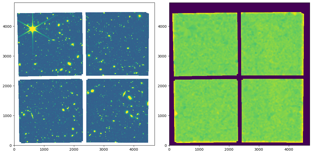
Let’s load the NIRCam F115W image and display it.

data = fits.getdata(fn1, ext=2)
snorm = SimpleNorm('sqrt', percent=98)
norm = snorm(data[data != 0])
fig, ax = plt.subplots(figsize=(10, 5))
_ = ax.imshow(data, norm=norm)

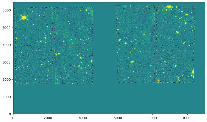
There are 2 NIRCam modules (A & B), each with 4 NIRCam short-wavelength (SW) detectors. All 8 SW detectors are 2k x 2k. There are also 2 2k x 2k long wavelength detectors, one covering each module. We see the SW detector gaps in each NIRCam module because these were parallel observations to NIRSpec prime observations. The prime observations had only very small dithers.

Data Units

The JWST calibration pipeline produces images in units of MJy/sr. The unit is stored in the FITS header in the BUNIT key.

header = fits.getheader(fn1, ext=2)
header['BUNIT']

'MJy/sr'

data_unit = u.Unit(header['BUNIT'])
data_unit

\[\mathrm{\frac{MJy}{sr}}\]

# another way to create the unit
u.MJy / u.sr

\[\mathrm{\frac{MJy}{sr}}\]

The pixel area in steradians is stored in the FITS header in the PIXAR_SR key.

header['PIXAR_SR']

2.11539874851881e-14

Let’s use Astropy units to calculate a scale factor to convert our original data in units of MJy/sr to μJy.

unit = u.uJy
unit_conv = ((1 * data_unit) * (header['PIXAR_SR'] * u.sr)).to(unit)
unit_conv

\[0.021153987 \; \mathrm{\mu Jy}\]

Load and Display the Data

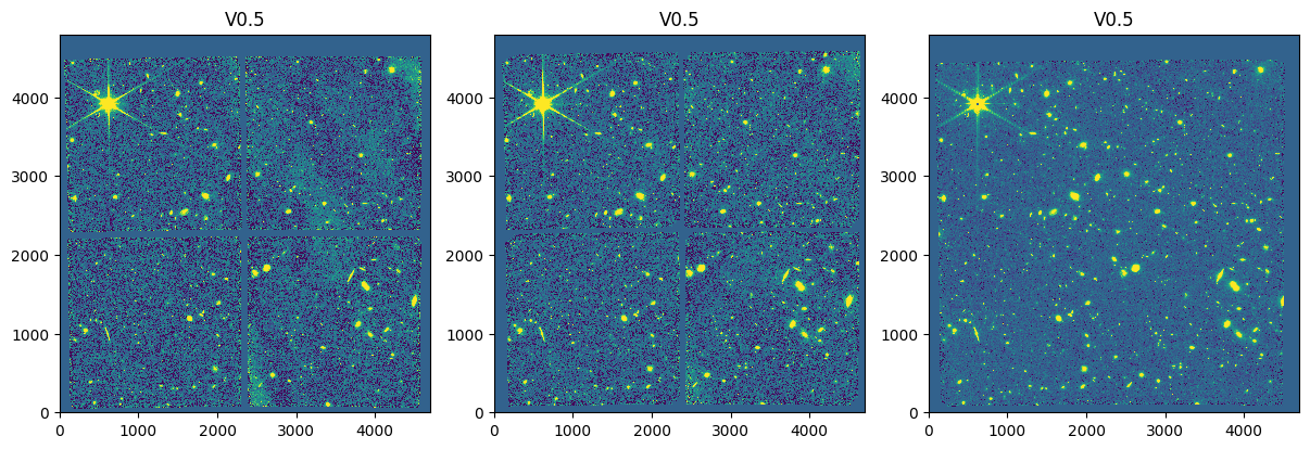
Let’s load the data. We’ll use only one of the NIRCam modules. We’ll also convert the units from MJy/sr to μJy.

# define a tuple of slice objects to extract only 1 NIRCam module
slc = (slice(1650, 6450), slice(0, 4700))


def load_data(filename):
    data = {}
    with fits.open(filename) as hdul:
        data['filter'] = filename.split('_')[6]
        data['sci_bksub'] = hdul[1].data[slc]
        data['sci'] = hdul[2].data[slc]
        data['err'] = hdul[3].data[slc]
        data['var_rnoise'] = hdul[7].data[slc]
        data['wcs'] = WCS(hdul[1].header)[slc]

        # convert the units in-place
        data['sci_bksub'] *= unit_conv.value
        data['sci_bksub'] <<= unit_conv.unit
        data['sci'] *= unit_conv.value
        data['sci'] <<= unit_conv.unit
        data['err'] *= unit_conv.value
        data['err'] <<= unit_conv.unit
        data['var_rnoise'] *= unit_conv.value ** 2
        data['var_rnoise'] <<= unit_conv.unit ** 2
    return data


f115w = load_data(fn1)
f200w = load_data(fn2)
f356w = load_data(fn3)
data = (f115w, f200w, f356w)

WARNING: FITSFixedWarning: 'datfix' made the change 'Set DATE-BEG to '2022-06-21T22:57:30.824' from MJD-BEG.
Set DATE-AVG to '2022-06-22T00:06:18.287' from MJD-AVG.
Set DATE-END to '2022-06-22T01:14:35.286' from MJD-END'. [astropy.wcs.wcs]
WARNING: FITSFixedWarning: 'obsfix' made the change 'Set OBSGEO-L to   -74.783957 from OBSGEO-[XYZ].
Set OBSGEO-B to   -36.777916 from OBSGEO-[XYZ].
Set OBSGEO-H to 1725421070.363 from OBSGEO-[XYZ]'. [astropy.wcs.wcs]

WARNING: FITSFixedWarning: 'datfix' made the change 'Set DATE-BEG to '2022-06-22T02:33:19.452' from MJD-BEG.
Set DATE-AVG to '2022-06-22T02:59:46.710' from MJD-AVG.
Set DATE-END to '2022-06-22T03:26:17.551' from MJD-END'. [astropy.wcs.wcs]
WARNING: FITSFixedWarning: 'obsfix' made the change 'Set OBSGEO-L to   -74.741833 from OBSGEO-[XYZ].
Set OBSGEO-B to   -36.807444 from OBSGEO-[XYZ].
Set OBSGEO-H to 1725573761.369 from OBSGEO-[XYZ]'. [astropy.wcs.wcs]

WARNING: FITSFixedWarning: 'datfix' made the change 'Set DATE-BEG to '2022-06-22T00:09:16.356' from MJD-BEG.
Set DATE-AVG to '2022-06-22T00:41:54.035' from MJD-AVG.
Set DATE-END to '2022-06-22T01:14:35.286' from MJD-END'. [astropy.wcs.wcs]
WARNING: FITSFixedWarning: 'obsfix' made the change 'Set OBSGEO-L to   -74.770114 from OBSGEO-[XYZ].
Set OBSGEO-B to   -36.787605 from OBSGEO-[XYZ].
Set OBSGEO-H to 1725471424.000 from OBSGEO-[XYZ]'. [astropy.wcs.wcs]

Let’s display the images.

snorm = SimpleNorm('sqrt', percent=98)
norm = snorm(data[2]['sci'].value)

nimg = len(data)
fig, ax = plt.subplots(ncols=nimg, figsize=(12, 4), constrained_layout=True)
for i in range(nimg):
    ax[i].imshow(data[i]['sci'].value, norm=norm)
    ax[i].set_title(data[i]['filter'].upper())

Background Subtraction

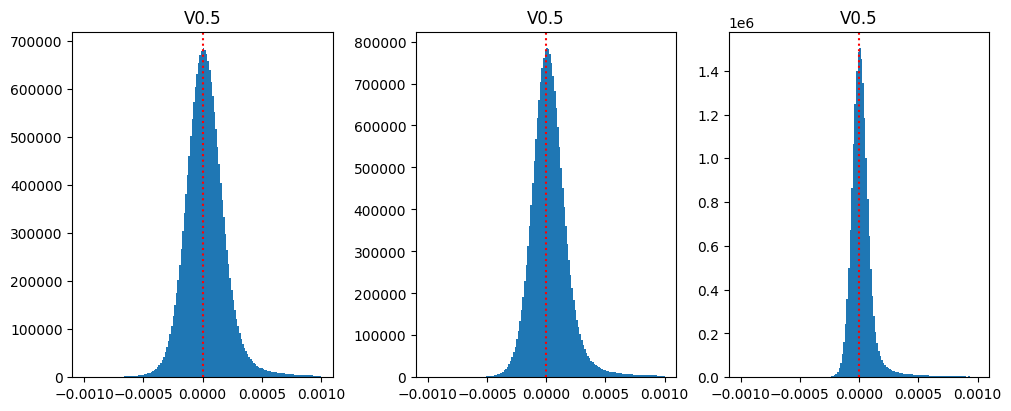
Let’s plot the histograms of the pixel values near zero to see if there is any background pedestal.

The CEERS team already subtracted a constant background value from each image.

fig, ax = plt.subplots(ncols=3, figsize=(10, 4))

for i in range(nimg):
    vals = data[i]['sci'].value
    vals = vals[vals != 0]
    ax[i].hist(vals, bins=150, range=(-0.001, 0.001))
    ax[i].set_title(data[i]['filter'].upper())
    ax[i].axvline(0, color='red', ls='dotted')

2D Background Estimation

To remove the varying residual background, we can use the photutils Background2D class.

This class can be used to estimate a 2D background and background RMS noise in an image.

The background is estimated using (sigma-clipped) statistics in each box of a grid that covers the input data to create a low-resolution background map.

The final background map is calculated by interpolating the low-resolution background map.

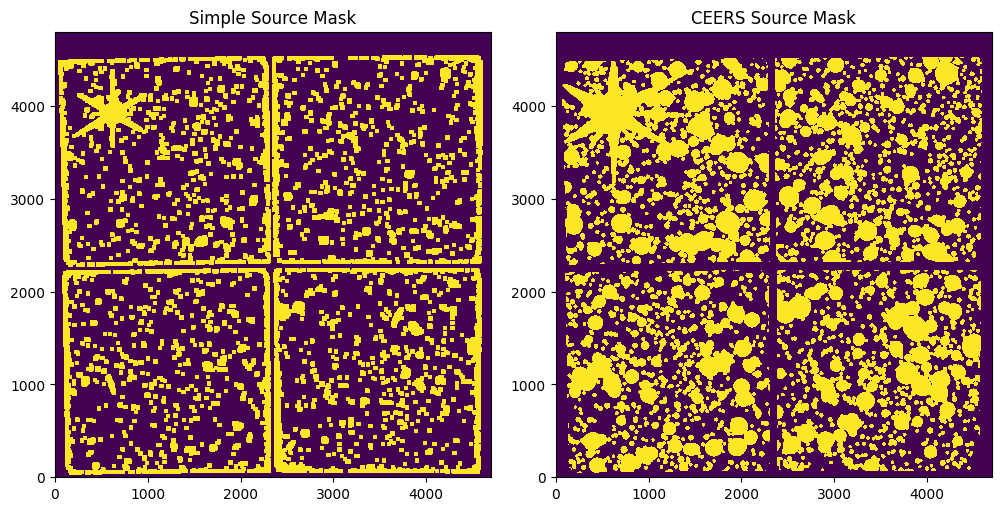
Source Mask

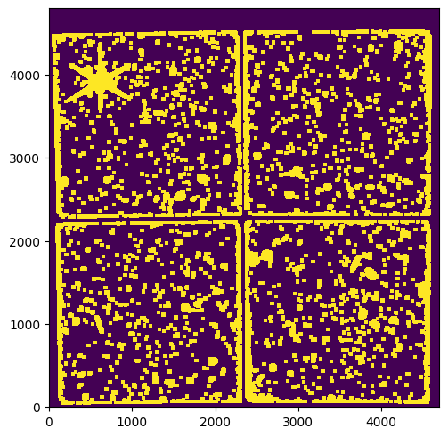
To get the best possible background estimate, we need to first create a mask of the sources in the image.

Let’s create a very rough source mask using a single threshold value. Here, we dilate the mask using a 45x45 pixel square footprint to include source wings in the mask.

mask = f115w['sci'].value > 0.001
mask = grey_dilation(mask, size=45)

fig, ax = plt.subplots()
_ = ax.imshow(mask)

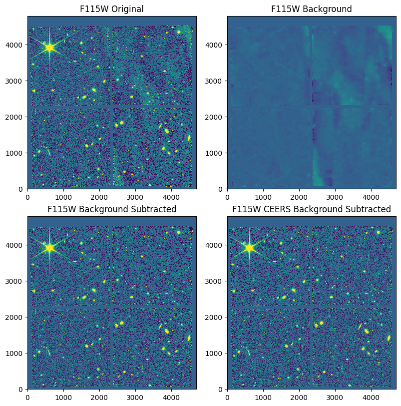
Background2D

bkg_estimator = BiweightLocationBackground()
bkgrms_estimator = BiweightScaleBackgroundRMS()
coverage_mask = f115w['sci'] == 0
bkg = Background2D(f115w['sci'], box_size=20, filter_size=5, exclude_percentile=90,
                   bkg_estimator=bkg_estimator, bkgrms_estimator=bkgrms_estimator,
                   coverage_mask=coverage_mask, mask=mask)
bkgim = bkg.background

fig, ax = plt.subplots(nrows=2, ncols=2, figsize=(8, 8))
ax = ax.ravel()
ax[0].imshow(f115w['sci'].value, norm=norm)
ax[0].set_title('F115W Original')
ax[1].imshow(bkgim.value, norm=norm)
ax[1].set_title('F115W Background')
ax[2].imshow((f115w['sci'] - bkgim).value, norm=norm)
ax[2].set_title('F115W Background Subtracted')
ax[3].imshow(f115w['sci_bksub'].value, norm=norm)
_ = ax[3].set_title('F115W CEERS Background Subtracted')

fits.info(fn1)

Filename: hlsp_ceers_jwst_nircam_nircam2_f115w_v0.5_i2d.fits
No.    Name      Ver    Type      Cards   Dimensions   Format
  0  PRIMARY       1 PrimaryHDU     374   ()      
  1  SCI_BKSUB     1 ImageHDU        76   (11000, 6450)   float64   
  2  SCI           1 ImageHDU        75   (11000, 6450)   float32   
  3  ERR           1 ImageHDU        10   (11000, 6450)   float32   
  4  CON           1 ImageHDU         9   (11000, 6450)   int32   
  5  WHT           1 ImageHDU         9   (11000, 6450)   float32   
  6  VAR_POISSON    1 ImageHDU         9   (11000, 6450)   float32   
  7  VAR_RNOISE    1 ImageHDU         9   (11000, 6450)   float32   
  8  VAR_FLAT      1 ImageHDU         9   (11000, 6450)   float32   
  9  BKGD          1 ImageHDU        39   (11000, 6450)   float64   
 10  BKGMASK       1 ImageHDU        39   (11000, 6450)   float32   
 11  HDRTAB        1 BinTableHDU    816   96R x 403C   [23A, 5A, 3A, 48A, 6A, 13A, 5A, 5A, 7A, 10A, 4A, L, D, D, D, D, 4A, 18A, 57A, 22A, 3A, D, 20A, D, 10A, 12A, 23A, 23A, 26A, 11A, 5A, 3A, 3A, 2A, 1A, 2A, 1A, L, 12A, 23A, 2A, 26A, 20A, 27A, 10A, K, L, L, L, L, 5A, 1A, 5A, D, D, D, D, D, D, D, D, D, D, 6A, 5A, 1A, 5A, 5A, 5A, L, D, D, D, D, D, D, D, D, D, D, D, D, 4A, D, D, D, D, D, D, D, D, D, K, 20A, 9A, D, D, D, D, D, D, D, D, D, 7A, D, D, K, K, D, D, K, K, D, D, K, K, K, K, K, D, D, D, D, D, D, D, D, K, K, L, L, K, K, D, D, D, D, D, D, D, 4A, K, K, K, K, K, K, D, D, D, D, 4A, D, D, K, D, K, D, D, D, D, D, D, D, D, D, D, D, D, D, D, D, D, D, 7A, 9A, D, D, D, D, D, D, D, D, D, D, D, D, D, 10A, 11A, D, D, D, D, D, D, D, D, D, D, D, D, K, K, D, 4A, K, K, K, D, 4A, K, K, K, D, 4A, K, D, D, K, 27A, 27A, 10A, D, D, D, D, D, D, D, 9A, 27A, D, D, D, D, D, D, D, 8A, 14A, 33A, D, D, 3A, 3A, D, 33A, 3A, 39A, D, D, 41A, 33A, 3A, 3A, 3A, 3A, 3A, D, 33A, 3A, 3A, 3A, D, D, 38A, 33A, 3A, 3A, D, 35A, 35A, D, 38A, D, 3A, D, D, D, D, 39A, D, D, D, 3A, D, 38A, D, 40A, 37A, D, D, D, 3A, D, D, D, D, D, 8A, D, D, D, D, D, 8A, 8A, D, D, D, D, D, 8A, D, 7A, 7A, D, D, 7A, 8A, D, D, 8A, D, D, D, 7A, D, 8A, 8A, 8A, 8A, 7A, D, D, 8A, 7A, D, D, D, D, 8A, D, 7A, D, D, D, 5A, D, L, 6A, D, D, D, D, 4A, D, D, D, K, D, D, D, D, D, D, 12A, 12A, D, 3A, 3A, D, D, D, D, D, D, D, D, D, D, D, D, D, D, D, D, D, 121A, D, D, D, D, D, D, K, D, D, D, D]   
 12  ASDF          1 BinTableHDU     11   1R x 1C   [36489B]   

Let’s load the CEERS source mask and show a comparison.

ceers_bkgmask = fits.getdata(fn1, ext=10)[slc]

fig, ax = plt.subplots(ncols=2, figsize=(10, 5))
ax[0].imshow(mask)
ax[0].set_title('Simple Source Mask')
ax[1].imshow(ceers_bkgmask.astype(bool) ^ coverage_mask)
_ = ax[1].set_title('CEERS Source Mask')

Let’s compute the background again, but this time we’ll use the CEERS source mask.

bkg = Background2D(f115w['sci'], box_size=10, filter_size=5,
                   exclude_percentile=90, coverage_mask=coverage_mask, mask=ceers_bkgmask,
                   bkg_estimator=bkg_estimator, bkgrms_estimator=bkgrms_estimator)
bkgim = bkg.background

fig, ax = plt.subplots(nrows=2, ncols=2, figsize=(8, 8))
ax = ax.ravel()
ax[0].imshow(f115w['sci'].value, norm=norm)
ax[0].set_title('F115W Original')
ax[1].imshow(bkgim.value, norm=norm)
ax[1].set_title('F115W Background')
ax[2].imshow((f115w['sci'] - bkgim).value, norm=norm)
ax[2].set_title('F115W Background Subtracted')
ax[3].imshow(f115w['sci_bksub'].value, norm=norm)
_ = ax[3].set_title('F115W CEERS Background Subtracted')

See the CEERS NIRCam GitHub repository for the scripts used for making the source mask and performing background subtraction.

We’ll use the CEERS background-subtracted (SCI_BKSUB) images for the rest of this tutorial.

Aperture Photometry

Photutils provides circular, elliptical, and rectangular aperture shapes (plus annulus versions of each).

Further, there are two types of aperture classes, defined either with pixel or sky (celestial) coordinates.

These are the names of the aperture classes that are defined in pixel coordinates:

• CircularAperture

• CircularAnnulus

• EllipticalAperture

• EllipticalAnnulus

• RectangularAperture

• RectangularAnnulus

The aperture classes defined in celestial coordinates have Sky prepended to their names:

• SkyCircularAperture

• SkyCircularAnnulus

• SkyEllipticalAperture

• SkyEllipticalAnnulus

• SkyRectangularAperture

• SkyRectangularAnnulus

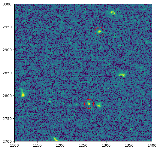
Define an Aperture Object

First, let’s define a circular aperture at the two given (x, y) pixel positions and radius (in pixels).

Photutils has many tools for detecting sources (e.g., see photutils.detection and photutils.segmentation) and measuring source positions (e.g., photutils.centroids). For this example, we’ll use estimated values based on cursor positions.

xypos = [(1262.9, 2781.4), (1285.9, 2939.3)]
aper = CircularAperture(xypos, r=10)
aper

<CircularAperture([[1262.9, 2781.4],
                 [1285.9, 2939.3]], r=10.0)>

fig, ax = plt.subplots(figsize=(6, 6))
ax.imshow(f115w['sci_bksub'].value, norm=norm)
aper.plot(ax=ax, color='red')
ax.set_xlim(1100, 1400)
_ = ax.set_ylim(2700, 3000)

aperture_photometry function

phot = aperture_photometry(f200w['sci_bksub'], aper, error=f200w['err'], wcs=f200w['wcs'])
phot

QTable length=2

id	xcenter	ycenter	sky_center	aperture_sum	aperture_sum_err
			deg,deg	uJy	uJy
int64	float64	float64	SkyCoord	float64	float64
1	1262.9	2781.4	214.92588919088467,52.941857419986555	0.07301065636369475	0.004254292010347718
2	1285.9	2939.3	214.92401980802305,52.94256387512347	0.06553649883660499	0.0042453372733323195

phot['aperture_mag'] = phot['aperture_sum'].to(u.ABmag)
phot

QTable length=2

id	xcenter	ycenter	sky_center	aperture_sum	aperture_sum_err	aperture_mag
			deg,deg	uJy	uJy	mag(AB)
int64	float64	float64	SkyCoord	float64	float64	float64
1	1262.9	2781.4	214.92588919088467,52.941857419986555	0.07301065636369475	0.004254292010347718	26.741534368116987
2	1285.9	2939.3	214.92401980802305,52.94256387512347	0.06553649883660499	0.0042453372733323195	26.858791909236327

Multiple positions and sizes

Multiple aperture objects can be input, BUT they must all have identical positions.

aper2 = CircularAperture(xypos, r=12)
aperture_photometry(f200w['sci_bksub'], (aper, aper2), error=f200w['err'], wcs=f200w['wcs'])

QTable length=2

id	xcenter	ycenter	sky_center	aperture_sum_0	aperture_sum_err_0	aperture_sum_1	aperture_sum_err_1
			deg,deg	uJy	uJy	uJy	uJy
int64	float64	float64	SkyCoord	float64	float64	float64	float64
1	1262.9	2781.4	214.92588919088467,52.941857419986555	0.07301065636369475	0.004254292010347718	0.07687332574886571	0.005082861205748076
2	1285.9	2939.3	214.92401980802305,52.94256387512347	0.06553649883660499	0.0042453372733323195	0.06555997520825779	0.005085923868101762

ApertureStats class

The ApertureStats calculates various statistics (including the sum) and properties using the pixels within the aperture.

Only one aperture object can be input.

apstats = ApertureStats(f200w['sci_bksub'], aper, error=f200w['err'], wcs=f200w['wcs'])
apstats

<photutils.aperture.stats.ApertureStats>
Length: 2

stats_tbl = apstats.to_table()
stats_tbl

QTable length=2

id	xcentroid	ycentroid	sky_centroid	sum	sum_err	sum_aper_area	center_aper_area	min	max	mean	median	mode	std	mad_std	var	biweight_location	biweight_midvariance	fwhm	semimajor_sigma	semiminor_sigma	orientation	eccentricity
			deg,deg	uJy	uJy	pix2	pix2	uJy	uJy	uJy	uJy	uJy	uJy	uJy	uJy2	uJy	uJy2	pix	pix	pix	deg
int64	float64	float64	SkyCoord	float64	float64	float64	float64	float64	float64	float64	float64	float64	float64	float64	float64	float64	float64	float64	float64	float64	float64	float64
1	1263.182663134733	2781.8937689404197	214.92588145725446,52.94185829141934	0.07301065636369475	0.004254292010347718	314.1592653589793	314.0	-0.00028889785282356555	0.0017084294994519121	0.0002322515426342805	0.0001366333865631305	-5.4602925579169464e-05	0.0003336793370397773	0.00019452316661150033	1.1134189996730531e-07	0.0001322520224237806	4.539571179364758e-08	7.333905702165728	3.357804823665577	2.850334712856219	-53.798303479855505	0.5286040913887978
2	1285.884955895828	2939.0652696702764	214.92402241551446,52.94256270339813	0.06553649883660499	0.0042453372733323195	314.1592653589793	313.0	-0.000279192322501696	0.0022059476840664083	0.00020927215554410338	9.157144209544037e-05	-0.00014382998480188565	0.0003873115937006317	0.00015816504936171956	1.500102706149232e-07	8.897633733574341e-05	3.047323059521578e-08	6.823977532697641	3.2047963996563666	2.554340576016742	7.165635563591646	0.603930778084528

The aperture statistics can also be accessed as attributes, e.g.,:

apstats.mean

\[[0.00023225154,~0.00020927216] \; \mathrm{\mu Jy}\]

Note that the returned measurements are for the input aperture position. ApertureStats returns the centroid value of the pixels within the input aperture, but the aperture is not recentered at the measured centroid position. However, you can create a new Aperture object using the measured centroid and then re-run ApertureStats.

Sky-based apertures

Sky-based apertures require an Astropy SkyCoord position and a size as an Astropy Quantity in angular units.

Sky apertures are not defined completely in sky coordinates. They simply use sky coordinates to define the central position, and the remaining parameters are converted to pixels using the pixel scale of the image at the central position. Projection distortions are not taken into account. They are not defined as apertures on the celestial sphere, but rather are meant to represent aperture shapes on an image. If the apertures were defined completely in sky coordinates, their shapes would not be preserved when converting to or from pixel coordinates.

xypos = [(1262.9, 2781.4), (1285.9, 2939.3)]
skycoord = f200w['wcs'].pixel_to_world(*np.transpose(xypos))
skycoord

<SkyCoord (ICRS): (ra, dec) in deg
    [(214.92588919, 52.94185742), (214.92401981, 52.94256388)]>

sky_aper = SkyCircularAperture(skycoord, r=0.3 * u.arcsec)
sky_aper

<SkyCircularAperture(<SkyCoord (ICRS): (ra, dec) in deg
    [(214.92588919, 52.94185742), (214.92401981, 52.94256388)]>, r=0.3 arcsec)>

When performing aperture photometry with a Sky-based aperture, a WCS transformation must be input.

phot = aperture_photometry(f200w['sci_bksub'], sky_aper, error=f200w['err'], wcs=f200w['wcs'])
phot

QTable length=2

id	xcenter	ycenter	sky_center	aperture_sum	aperture_sum_err
			deg,deg	uJy	uJy
int64	float64	float64	SkyCoord	float64	float64
1	1262.8999999992702	2781.4000000001824	214.92588919088467,52.941857419986555	0.0730107122935297	0.0042543119728190954
2	1285.899999997282	2939.3000000007023	214.92401980802305,52.94256387512347	0.06553656428045805	0.00424535734794874

Creating a multiband segmentation-based catalog

Creating a Detection Image

We are ready to detect sources in our multiband data, but which image do we use? Typically, that depends on your science use case. For example, perhaps you are interested in Lyman-break dropout galaxies, in which case a redder filter or filters is more appropriate.

One other consideration is the varying PSF across our multiband data where the PSF is broader at redder-wavelengths (R ~ λ / D). One method to address this is to PSF match all the multiband data to a common PSF (usually the reddest band with the broadest PSF). A common technique is to generate a set of matching kernels that are then convolved with the images, blurring them all to the same resolution as the reddest band. See Photutils PSF Matching for tools to create matching kernels. We do not PSF match our multiband data in the examples that follow.

In general, one should use a detection image with a high signal-to-noise ratio. A common case is to create a deep detection image by combining the images in several filters. We can do this by creating an inverse-variance weighted combination of images. For this example, we’ll use all three filter images. The weights will be the inverse variance of the read noise (the read noise variance is in the VAR_RNOISE extension).

scis = [filt['sci_bksub'] for filt in data]
whts = [1.0 / filt['var_rnoise'] for filt in data]
detimg = np.multiply(scis, whts).sum(axis=0) / np.sum(whts, axis=0) << unit
scis = None  # free memory
whts = None

/tmp/ipykernel_2196/3398041919.py:3: RuntimeWarning: invalid value encountered in divide
  detimg = np.multiply(scis, whts).sum(axis=0) / np.sum(whts, axis=0) << unit

fig, ax = plt.subplots(figsize=(6, 6))
_ = ax.imshow(detimg.value, norm=norm)

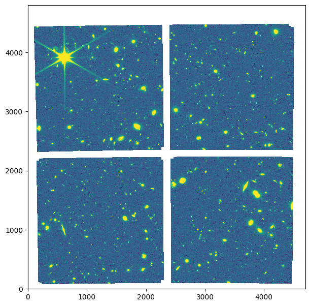
Image Segmentation (Source Extraction)

Image segmentation is a process of assigning a label to every pixel in an image, such that pixels with the same label are part of the same source. Detected sources must have a minimum number of connected pixels that are each greater than a specified threshold value in an image.

The threshold level is usually defined as a multiple of the background noise (sigma level) above the background. This can be specified either as a per-pixel threshold image or a single threshold value for the whole image.

The image is often filtered before thresholding to smooth the noise and maximize the detectability of objects with a shape similar to the filter kernel.

Let’s convolve the background-subtracted detection image with a 2D Gaussian kernel with a FWHM of 3 pixels.

kernel_fwhm = 3.0
kernel_size = int(kernel_fwhm * 2 + 1)
kernel = make_2dgaussian_kernel(kernel_fwhm, size=kernel_size)
detconv = convolve(detimg, kernel, mask=coverage_mask)

WARNING: nan_treatment='interpolate', however, NaN values detected post convolution. A contiguous region of NaN values, larger than the kernel size, are present in the input array. Increase the kernel size to avoid this. [astropy.convolution.convolve]

coverage_mask = np.isnan(detimg)
bkg = Background2D(detimg, box_size=10, filter_size=5,
                   exclude_percentile=90, coverage_mask=coverage_mask, mask=ceers_bkgmask,
                   bkg_estimator=bkg_estimator, bkgrms_estimator=bkgrms_estimator)
bkgrms = bkg.background_rms

fig, ax = plt.subplots(ncols=2, figsize=(12, 6))
ax[0].imshow(detconv.value, norm=norm)
norm2 = simple_norm(bkgrms.value, 'sqrt', percent=99)
_ = ax[1].imshow(bkgrms.value, norm=norm2)

Next, we need to define the detection threshold. In this example, we’ll define a 2D detection threshold image using the background RMS image calculated above. We set the threshold at the 4.0\(\sigma\) (per pixel) noise level (above the background).

threshold = bkgrms * 4.0
np.median(threshold)

\[0.0001850487 \; \mathrm{\mu Jy}\]

Now we are ready to detect the sources in the background-subtracted convolved image. Let’s find sources that have at least 25 connected pixels that are each greater than the corresponding threshold level defined above. For this, we use the detect_sources function.

mask = np.isnan(detimg)
npixels = 25
segm = detect_sources(detconv, threshold, npixels=npixels, mask=mask)
segm

<photutils.segmentation.core.SegmentationImage>
shape: (4800, 4700)
nlabels: 1785
labels: [   1    2    3    4    5 ... 1781 1782 1783 1784 1785]

The result is a segmentation image (SegmentationImage object). The segmentation image is an array with the same size as the science image, in which each detected source is labeled with a unique integer value (>= 1). Background pixels have a value of 0. As a simple example, a segmentation map containing two distinct sources (labeled 1 and 2) might look like this:

0 0 0 0 0 0 0 0 0 0
0 1 1 0 0 0 0 0 0 0
1 1 1 1 1 0 0 0 2 0
1 1 1 1 0 0 0 2 2 2
1 1 1 0 0 0 2 2 2 2
1 1 1 1 0 0 0 2 2 0
1 1 0 0 0 0 2 2 0 0
0 1 0 0 0 0 2 0 0 0
0 0 0 0 0 0 0 0 0 0

where all the pixels labeled 1 belong to the first source, all those labeled 2 belong to the second, and all those labeled 0 are background pixels.

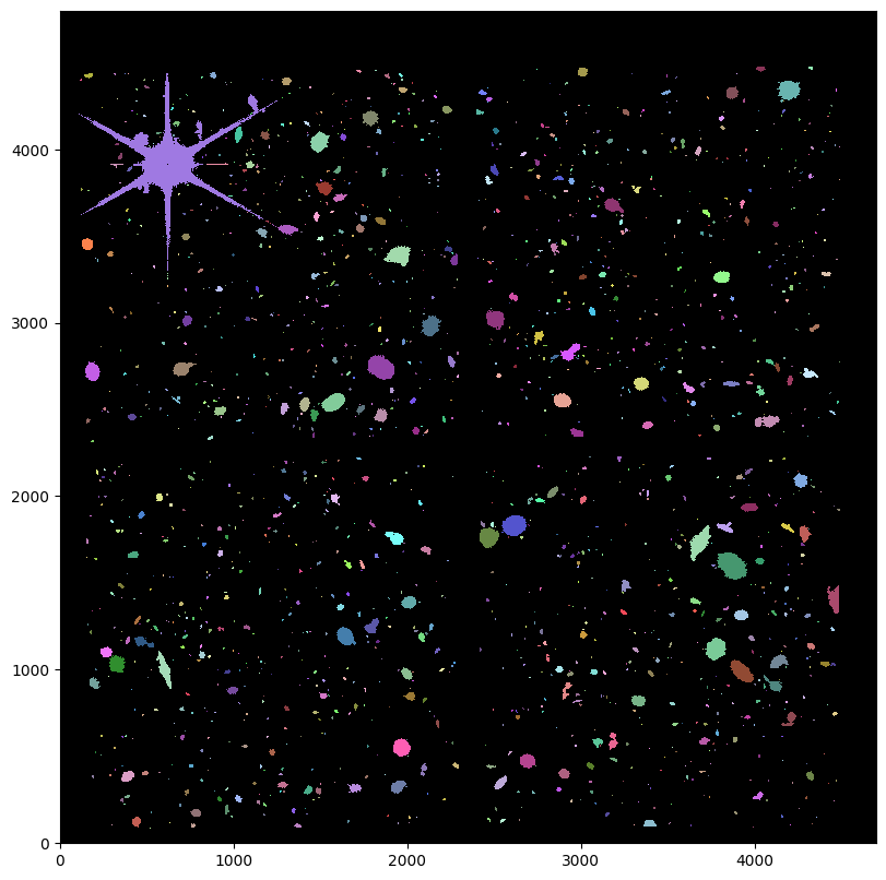
Let’s plot the segmentation image.

fig, ax = plt.subplots(figsize=(8, 8))
_ = segm.imshow(ax=ax)

Let’s plot the segmentation image next to the science image.

# switch to interactive plots
%matplotlib widget

fig, ax = plt.subplots(ncols=2, figsize=(12, 6), sharex=True, sharey=True)
ax[0].imshow(detconv.value, norm=norm)
ax[0].set_title('Detection Image')
segm.imshow(ax=ax[1])
_ = ax[1].set_title('Segmentation Image')

We can use the plot_patches SegmentationImage method to plot the segmentation outlines on the science image.

This is a good way to inspect the source extraction. The source detection parameters (e.g., threshold, npixels) can be adjusted as needed.

fig, ax = plt.subplots(figsize=(8, 8))
ax.imshow(detimg.value, norm=norm)
_ = segm.plot_patches(ax=ax)

The SegmentationImage object has attributes that can give various properties of the source segments.

star_label = segm.data[3852, 612]
idx = segm.get_index(label=star_label)
sobj = segm.segments[idx]
sobj.area, sobj.bbox, sobj.slices

(np.int64(149684),
 BoundingBox(ixmin=106, ixmax=1251, iymin=3297, iymax=4438),
 (slice(3297, 4438, None), slice(106, 1251, None)))

sobj.polygon

Source deblending

Comparing the data array with the segmentation image, we see that several detected sources were blended together. We can deblend them using the deblend_sources function, which uses a combination of multi-thresholding and watershed segmentation.

The deblending can be controlled with the deblend_sources keywords:

• nlevels is the number of multi-thresholding levels to use; larger values give more deblending, but longer runtime

• contrast is the fraction (0 - 1) of the total source flux that a local peak must have to be considered as a separate object

  • contrast = 1: no deblending

  • contrast = 0: max deblending

• mode is the mode used in defining the spacing of the nlevels (‘exponential’, ‘linear’, ‘sinh’)

The npixels and connectivity values should match those used in detect_sources.

npixels2 = 9
segm_deblended = deblend_sources(detconv, segm, npixels=npixels2, progress_bar=True)

segm.nlabels, segm_deblended.nlabels, segm_deblended

(1785,
 2172,
 <photutils.segmentation.core.SegmentationImage>
 shape: (4800, 4700)
 nlabels: 2172
 labels: [   1    2    3    4    5 ... 2168 2169 2170 2171 2172])

fig, ax = plt.subplots(ncols=2, figsize=(12, 6), sharex=True, sharey=True)
segm.imshow(ax=ax[0])
ax[0].set_title('Original Segmentation Image')
segm_deblended.imshow(ax=ax[1])
_ = ax[1].set_title('Deblended Segmentation Image')

label = segm.data[1597, 3877]
idx = segm.get_index(label=label)
slc2 = segm.slices[idx]

fig, ax = plt.subplots(ncols=2, nrows=2, figsize=(10, 6))
ax = ax.ravel()
norm3 = simple_norm(detconv[slc2].value, 'sqrt', percent=98)
ax[0].imshow(detconv[slc2].value, norm=norm3)
ax[0].set_title('Detection Image')
segm[slc2].imshow(ax=ax[1])
ax[1].set_title('Segmentation Image')
segm_deblended[slc2].imshow(ax=ax[2])
ax[2].set_title('Deblended Segmentation Image')
ax[3].imshow(detimg[slc2].value, norm=norm3)
_ = segm_deblended[slc2].imshow(ax=ax[3], alpha=0.2)

child_labels = segm_deblended.deblended_labels_inverse_map[label]
child_labels

array([1749, 1750, 1751], dtype=int32)

segm_deblended.deblended_labels_map[child_labels[0]]

np.int32(577)

Modifying a Segmentation Image

The SegmentationImage object provides several methods that can be used to modify itself (e.g., combining labels, removing labels, removing border segments) prior to measuring source photometry and other source properties, including:

• reassign_labels: Reassign one or more label numbers.

• relabel_consecutive: Reassign the label numbers consecutively, such that there are no missing label numbers.

• keep_labels: Keep only the specified labels.

• remove_labels: Remove one or more labels.

• remove_border_labels: Remove labeled segments near the image border.

• remove_masked_labels: Remove labeled segments located within a masked region.

Let’s combine the deblended segments of the bright star.

star_label = segm.data[3852, 612]
child_labels = segm_deblended.deblended_labels_inverse_map[star_label]
child_labels

array([2003, 2004, 2005, 2006, 2007, 2008, 2009, 2010, 2011, 2012, 2013,
       2014, 2015, 2016, 2017, 2018, 2019], dtype=int32)

But, we’ll exclude the labels which are galaxies.

xy_exclude = ((462, 4059), (495, 3770), (807, 4100), (1110, 4270))
x_exclude, y_exclude = np.transpose(xy_exclude)
exclude_labels = segm_deblended.data[y_exclude, x_exclude]
exclude_labels

array([2014, 2004, 2017, 2019], dtype=int32)

keep_labels = np.setdiff1d(child_labels, exclude_labels)
keep_labels

array([2003, 2005, 2006, 2007, 2008, 2009, 2010, 2011, 2012, 2013, 2015,
       2016, 2018], dtype=int32)

segm_deblended.reassign_labels(keep_labels, keep_labels[0])
fig, ax = plt.subplots(ncols=2, figsize=(12, 6), sharex=True, sharey=True)
segm.imshow(ax=ax[0])
ax[0].set_title('Original Segmentation Image')
segm_deblended.imshow(ax=ax[1])
_ = ax[1].set_title('Deblended Segmentation Image')

Let’s use the remove_label method to remove the bright star from the segmentation image.

segm_deblended.remove_label(keep_labels[0])
_ = segm_deblended.imshow(figsize=(8, 8))

When we combined and then removed segments, our segment labels are no longer consecutive.

segm_deblended

<photutils.segmentation.core.SegmentationImage>
shape: (4800, 4700)
nlabels: 2159
labels: [   1    2    3    4    5 ... 2168 2169 2170 2171 2172]

segm_deblended.is_consecutive

np.False_

segm_deblended.missing_labels

array([2003, 2005, 2006, 2007, 2008, 2009, 2010, 2011, 2012, 2013, 2015,
       2016, 2018])

segm_deblended.relabel_consecutive()
segm_deblended.is_consecutive

np.True_

segm_deblended

<photutils.segmentation.core.SegmentationImage>
shape: (4800, 4700)
nlabels: 2159
labels: [   1    2    3    4    5 ... 2155 2156 2157 2158 2159]

SourceFinder class

The SourceFinder class is a convenience class that combines the functionality of detect_sources and deblend_sources. After defining the SourceFinder object with the desired detection and deblending parameters, you call it with the background-subtracted (convolved) image and threshold.

# finder = SourceFinder(npixels=(npixels, npixels2), deblend=True, progress_bar=True)
# segment_map = finder(detconv, threshold, mask=mask)

Source Catalog: Photometry, Centroids, and Shape Properties

The SourceCatalog class is used to measure the photometry, centroids, and shape/morphological properties of sources defined in a segmentation image. In its most basic form, it takes as input the (background-subtracted) image and the segmentation image. Usually the convolved image is also input, from which the source centroids and shape/morphological properties are measured (if not input, the unconvolved image is used instead).

First, we create a catalog from the detection image.

det_cat = SourceCatalog(detimg, segm_deblended, convolved_data=detconv, wcs=f356w['wcs'])
det_cat

<photutils.segmentation.catalog.SourceCatalog>
Length: 2159
labels: [   1    2    3    4    5 ... 2155 2156 2157 2158 2159]

Our det_cat variable is a SourceCatalog object for the detection image.

The properties of each source can be accessed using SourceCatalog attributes, or they can be output to an Astropy QTable using the to_table method.

Please see the SourceCatalog documentation for a complete list of the available source properties.

The to_table method is used to create a table of source measurements. The output is an Astropy QTable.

Each row in the table represents a source. The columns represent the calculated source properties. The label column corresponds to the label value in the input segmentation image.

det_tbl = det_cat.to_table()
det_tbl

QTable length=2159

label	xcentroid	ycentroid	sky_centroid	bbox_xmin	bbox_xmax	bbox_ymin	bbox_ymax	area	semimajor_sigma	semiminor_sigma	orientation	eccentricity	min_value	max_value	local_background	segment_flux	segment_fluxerr	kron_flux	kron_fluxerr
			deg,deg					pix2	pix	pix	deg		uJy	uJy	uJy	uJy	uJy	uJy	uJy
int32	float64	float64	SkyCoord	int64	int64	int64	int64	float64	float64	float64	float64	float64	float64	float64	float64	float64	float64	float64	float64
1	519.5949551476	81.07259985155056	214.9609852444238,52.93199215314523	514	526	79	85	70.0	2.8724692637820226	1.6659138838634198	-11.32056036890879	0.8146457926275532	0.00019159071058753358	0.001428366586564793	0.0	0.04308027658363421	nan	0.06576522534470572	nan
2	766.489104864343	98.5324969870587	214.958588880522,52.930519822928666	751	783	84	114	616.0	3.223952014289902	3.0667313116773425	7.592654136025441	0.3084716162296652	9.359696794881929e-05	0.24056629093773663	0.0	2.95442525875817	nan	2.8678235574541024	nan
3	1371.2527175709843	96.86878719989326	214.95318743218436,52.92667318326436	1348	1393	89	113	758.0	7.85770279122408	4.288892164291958	-18.4546953020117	0.8379023885500212	0.0001672576413085766	0.010548932295279147	0.0	1.1038019934971528	nan	1.1939369727423381	nan
4	3991.2361362338893	91.39582056328483	214.9297798430202,52.91001512387632	3988	3995	90	94	31.0	1.7366670948689087	1.2098242412307103	-0.8145125549258665	0.717425080735856	0.00016757073025512964	0.0014933341623335412	0.0	0.02059214366044146	nan	0.029888712810003045	nan
5	1845.8371113784754	94.04547140465078	214.94896532719426,52.92364618769537	1842	1850	93	96	26.0	1.8816545423799809	1.0085658346537048	-3.9468821829730807	0.8442183187697342	0.0002417399418735864	0.001150213438969466	0.0	0.01713613686714633	nan	0.026092613208891995	nan
6	3635.1881224871945	99.55083655878093	214.93288180058389,52.91231919315401	3632	3638	93	105	61.0	3.0885160380015795	1.4286982806507114	-84.77379556308978	0.8865754280970479	0.00017424833451930636	0.001109478099035839	0.0	0.03192307777654567	nan	0.05332255562080552	nan
7	295.4795965787447	102.4665003529108	214.962768593605,52.9335297918858	293	298	100	105	28.0	1.6296715069576206	1.2709620049314665	-44.63440099284509	0.6259185146852972	0.0002687265461240606	0.0004893651918458313	0.0	0.009962071053491717	nan	0.04345487771200407	nan
8	4205.705778270739	102.9133784138537	214.92773856854785,52.90871590639413	4203	4209	100	106	36.0	1.898192921978675	1.3299138437998494	-45.34160135098274	0.7135336005715309	0.00018294945082797953	0.0009696728063750856	0.0	0.0195639354282886	nan	0.039308957758529224	nan
9	3307.19135160857	103.9118439804293	214.93577283474275,52.91442464721972	3304	3310	101	107	37.0	1.6950016829397712	1.4208569341215362	-45.7976523419878	0.5452663584009633	0.00019069496342542382	0.0013027748999248012	0.0	0.022784642264923285	nan	0.04245106751305349	nan
...	...	...	...	...	...	...	...	...	...	...	...	...	...	...	...	...	...	...	...
2151	1318.2010455639638	4316.597489502455	214.9092191179457,52.94979345128564	1315	1321	4314	4319	28.0	1.9608434276217235	1.0855121841007276	42.73948260457702	0.832786348899688	0.0001734128853711693	0.00027173965327833394	0.0	0.006278585485429527	nan	0.06936167100627669	nan
2152	1326.9610337188283	4321.127609327313	214.90909290798857,52.94976228281462	1322	1332	4317	4325	47.0	2.9919226615929686	1.2766956373209077	37.34559508540399	0.9043865667779264	0.00012142170532841704	0.00038147403938045243	0.0	0.011397181107809979	nan	0.11311127078505667	nan
2153	494.18629454454964	4356.882692399877	214.91617701196415,52.95524252166971	483	509	4348	4367	322.0	4.802433709834651	2.967285601212213	-29.23888779897383	0.7862793071288311	8.164345073692908e-05	0.004815354253990144	0.0	0.2230271656583786	nan	0.2522678067290374	nan
2154	511.98435163837223	4351.301582630822	214.91607635443594,52.955099400845555	509	515	4349	4354	30.0	1.531762742066521	1.4459883452397193	-12.816075744140154	0.3299373869918721	0.0001601738349328719	0.00044793747862894776	0.0	0.007743445295495495	nan	0.02312506126273308	nan
2155	157.78560945089197	4423.995466755786	214.9184840929336,52.957740471763806	134	173	4406	4431	678.0	6.005626036478682	4.84632869559215	-4.671651805550406	0.5905995624961892	0.0001292017832083356	0.01660979479113312	0.0	1.4775174649673248	nan	1.6150349646531366	nan
2156	171.63013181469057	4424.209996831193	214.91835777129148,52.95765373771049	166	189	4407	4431	447.0	5.0159398959072625	4.187121111769937	-39.16885151544841	0.5506093972931239	0.00012093154720116209	0.009900229759029303	0.0	0.7222632382815204	nan	0.8029248567175558	nan
2157	4034.3331925957636	4467.067753876071	214.88331213554403,52.933357468139306	4008	4061	4442	4471	1130.0	6.776549383926935	5.161440263081692	-2.6880048692233167	0.6479745163802223	5.105626814252766e-05	0.1595613980379308	0.0	1.934904479369893	nan	1.8738664801357052	nan
2158	4002.580651209752	4454.295761364674	214.88373092850094,52.933490227483496	4000	4005	4453	4456	17.0	1.3647906834956405	0.9326206586624367	5.7113746701017725	0.7300971476645636	0.00010922046253814311	0.0003617963616611741	0.0	0.004565197407073732	nan	0.036476416958664	nan
2159	4009.6154765805786	4453.691872786995	214.88367432364515,52.93344229031217	4006	4014	4451	4456	33.0	2.0677950414707356	1.3282068385967711	-2.932734198589163	0.7664281703326615	0.00010425588602476812	0.0003687716022665888	0.0	0.008087272713176982	nan	0.066641109156109	nan

The output columns can be customized using the optional columns keyword.

columns = ('label', 'xcentroid', 'ycentroid', 'area', 'segment_flux', 'kron_flux')
det_tbl2 = det_cat.to_table(columns=columns)
det_tbl2

QTable length=2159

label	xcentroid	ycentroid	area	segment_flux	kron_flux
			pix2	uJy	uJy
int32	float64	float64	float64	float64	float64
1	519.5949551476	81.07259985155056	70.0	0.04308027658363421	0.06576522534470572
2	766.489104864343	98.5324969870587	616.0	2.95442525875817	2.8678235574541024
3	1371.2527175709843	96.86878719989326	758.0	1.1038019934971528	1.1939369727423381
4	3991.2361362338893	91.39582056328483	31.0	0.02059214366044146	0.029888712810003045
5	1845.8371113784754	94.04547140465078	26.0	0.01713613686714633	0.026092613208891995
6	3635.1881224871945	99.55083655878093	61.0	0.03192307777654567	0.05332255562080552
7	295.4795965787447	102.4665003529108	28.0	0.009962071053491717	0.04345487771200407
8	4205.705778270739	102.9133784138537	36.0	0.0195639354282886	0.039308957758529224
9	3307.19135160857	103.9118439804293	37.0	0.022784642264923285	0.04245106751305349
...	...	...	...	...	...
2151	1318.2010455639638	4316.597489502455	28.0	0.006278585485429527	0.06936167100627669
2152	1326.9610337188283	4321.127609327313	47.0	0.011397181107809979	0.11311127078505667
2153	494.18629454454964	4356.882692399877	322.0	0.2230271656583786	0.2522678067290374
2154	511.98435163837223	4351.301582630822	30.0	0.007743445295495495	0.02312506126273308
2155	157.78560945089197	4423.995466755786	678.0	1.4775174649673248	1.6150349646531366
2156	171.63013181469057	4424.209996831193	447.0	0.7222632382815204	0.8029248567175558
2157	4034.3331925957636	4467.067753876071	1130.0	1.934904479369893	1.8738664801357052
2158	4002.580651209752	4454.295761364674	17.0	0.004565197407073732	0.036476416958664
2159	4009.6154765805786	4453.691872786995	33.0	0.008087272713176982	0.066641109156109

Here, we access a few of the source properties as attributes of the SourceCatalog object. These get returned as NumPy arrays or Astropy objects (e.g., SkyCoord, Quantity).

det_cat.xcentroid, det_cat.sky_centroid, det_cat.segment_flux, det_cat.orientation

(array([ 519.59495515,  766.48910486, 1371.25271757, ..., 4034.3331926 ,
        4002.58065121, 4009.61547658], shape=(2159,)),
 <SkyCoord (ICRS): (ra, dec) in deg
     [(214.96098524, 52.93199215), (214.95858888, 52.93051982),
      (214.95318743, 52.92667318), ..., (214.88331214, 52.93335747),
      (214.88373093, 52.93349023), (214.88367432, 52.93344229)]>,
 <Quantity [0.04308028, 2.95442526, 1.10380199, ..., 1.93490448, 0.0045652 ,
            0.00808727] uJy>,
 <Quantity [-11.32056037,   7.59265414, -18.4546953 , ...,  -2.68800487,
              5.71137467,  -2.9327342 ] deg>)

Multiband Catalog

Now let’s perform the photometry on each of the filter images. We pass in the science and (total) error array for each band, plus the segmentation image and the detection catalog SourceCatalog object created above. We need to input the detection catalog to ensure that the aperture centroids (and shapes for Kron apertures) are the same for all the bands.

f115w_cat = SourceCatalog(f115w['sci_bksub'], segm_deblended, error=f115w['err'], detection_cat=det_cat)
f200w_cat = SourceCatalog(f200w['sci_bksub'], segm_deblended, error=f200w['err'], detection_cat=det_cat)
f356w_cat = SourceCatalog(f356w['sci_bksub'], segm_deblended, error=f356w['err'], detection_cat=det_cat)

By default, the SourceCatalog class computes only “segment” (isophotal) photometry and Kron (elliptical aperture) photometry. We can also compute circular aperture photometry at various radii using the circular_photometry method.

f115w_cat.circular_photometry(radius=5, name='circ_rad5')
f115w_cat.circular_photometry(radius=10, name='circ_rad10')
f200w_cat.circular_photometry(radius=5, name='circ_rad5')
f200w_cat.circular_photometry(radius=10, name='circ_rad10')
f356w_cat.circular_photometry(radius=5, name='circ_rad5')
_ = f356w_cat.circular_photometry(radius=10, name='circ_rad10')

columns = ['segment_flux', 'segment_fluxerr', 'kron_flux', 'kron_fluxerr', 
           'circ_rad5_flux', 'circ_rad5_fluxerr', 'circ_rad10_flux', 'circ_rad10_fluxerr']
f115w_tbl = f115w_cat.to_table(columns=columns)
f200w_tbl = f200w_cat.to_table(columns=columns)
f356w_tbl = f356w_cat.to_table(columns=columns)

def add_magnitudes(tbl):
    for col in tbl.colnames:
        if col.endswith('flux'):
            fluxerr_col = col.replace('flux', 'fluxerr')
            flux = tbl[col]
            fluxerr = tbl[fluxerr_col]

            mag = -2.5 * np.log10(flux.value) + 23.9
            magerr = -2.5 * np.log10(1.0 + (flux / fluxerr))

            # set negative flux to the 2-sigma upper limit
            idx = flux.value <= 0
            mag[idx] = -2.5 * np.log10(2.0 * fluxerr[idx].value) + 23.9
            magerr[idx] = np.nan

            magcol = col.replace('flux', 'mag')
            magerrcol = f'{magcol}err'
            tbl[magcol] = mag * u.mag
            tbl[magerrcol] = magerr * u.mag
    return tbl


f115w_tbl = add_magnitudes(f115w_tbl)
f200w_tbl = add_magnitudes(f200w_tbl)
f356w_tbl = add_magnitudes(f356w_tbl)

/tmp/ipykernel_2196/270370035.py:8: RuntimeWarning: invalid value encountered in log10
  mag = -2.5 * np.log10(flux.value) + 23.9
/opt/hostedtoolcache/Python/3.11.13/x64/lib/python3.11/site-packages/astropy/units/quantity.py:659: RuntimeWarning: invalid value encountered in log10
  result = super().__array_ufunc__(function, method, *arrays, **kwargs)

def prefix_flux_columns(tbl, prefix):
    for col in tbl.colnames:
        if col != 'label':
            tbl.rename_column(col, f'{prefix}_{col}')
    return tbl


f115w_tbl = prefix_flux_columns(f115w_tbl, 'f115w')
f200w_tbl = prefix_flux_columns(f200w_tbl, 'f200w')
f356w_tbl = prefix_flux_columns(f356w_tbl, 'f356w')

f115w_tbl

QTable length=2159

f115w_segment_flux	f115w_segment_fluxerr	f115w_kron_flux	f115w_kron_fluxerr	f115w_circ_rad5_flux	f115w_circ_rad5_fluxerr	f115w_circ_rad10_flux	f115w_circ_rad10_fluxerr	f115w_segment_mag	f115w_segment_magerr	f115w_kron_mag	f115w_kron_magerr	f115w_circ_rad5_mag	f115w_circ_rad5_magerr	f115w_circ_rad10_mag	f115w_circ_rad10_magerr
uJy	uJy	uJy	uJy	uJy	uJy	uJy	uJy	mag	mag	mag	mag	mag	mag	mag	mag
float64	float32	float64	float64	float64	float64	float64	float64	float64	float64	float64	float64	float64	float64	float64	float64
0.026460426740559803	0.0032706984784454107	0.12324922551804493	0.009012583377638087	0.042191518584833866	0.0036035016289898995	0.12036723112548395	0.007329379389860909	27.843507890018323	-2.39642709282544	26.173039502729186	-2.916462906453287	27.336937107311787	-2.7602338308236507	26.1987293241901	-3.1027804180285443
6.244690540584277	0.012532574124634266	6.067022200080507	0.011331418005816619	5.502765951399317	0.009393388798709573	5.990589418443795	0.010946114229381016	21.911222696205645	-6.745853397505529	21.94256103977239	-6.823754254224386	22.048547396500815	-6.921248661993338	21.956326112397267	-6.847506014417105
1.2071897629216368	0.010385734029114246	1.565155056862051	0.016626896350257145	0.4264926433406219	0.0036790865011461613	0.9422609528015482	0.007172343338964137	23.695561140183333	-5.172646757820458	23.413606578195072	-4.9458385670986775	24.825221139166867	-5.169754667472417	23.96457201407072	-5.304508467844126
0.01382632513730629	0.0023898258805274963	0.02490894407793871	0.00564602263737409	0.020668602431692558	0.0038219054555943574	0.02150233954912273	0.007562914161846576	28.54823308636185	-2.0789538005231973	27.90911170593235	-1.833347999679242	28.111722221194732	-2.0167946304568303	28.068785710909054	-1.4617123675908354
0.019378308042289072	0.002250947989523411	0.05116464011355557	0.005481938641675988	0.044819733303353954	0.00388722337127222	0.056484495525558384	0.007550613123659261	28.181710361811596	-2.456690303105512	27.12757519076435	-2.5355987873774657	27.271326830079495	-2.7448787437313205	27.020176864157296	-2.321089830406173
0.03165638615029799	0.002962352242320776	0.04266565391181901	0.008138555464324328	0.031052109463903244	0.0032573311922548982	0.04703979991160488	0.007047895315392655	27.64884666276858	-2.669186348183196	27.32480398449952	-1.988380924094622	27.669772228862257	-2.5563792993327104	27.218836335605236	-2.212597577589724
0.011225859701148675	0.0016454276628792286	0.06280336255351039	0.006229392712415807	0.023761238793316	0.0027262532617987286	0.056409289562673534	0.005498391547833056	28.774450974549215	-2.233357980217559	26.9050427577215	-2.6115237425626985	27.96032730284277	-2.4686866031461547	27.021623424722748	-2.628772183884135
0.023146646975483774	0.002095666015520692	0.030584078415906713	0.005616101946925867	0.026926470695427706	0.0030485768670560198	0.032420473711858314	0.006071371141937934	27.988779780028956	-2.7020176918992913	27.68626150370067	-2.023189378957552	27.824551416689108	-2.481656827627455	27.62295160936473	-2.005204861528172
0.029256612804497883	0.002119420561939478	0.04454697186038396	0.005926797303094583	0.03246735243482099	0.0030271803094493377	0.04459772741282991	0.006105539901279711	27.734439889773824	-2.9259522369074387	27.277954530920887	-2.3256141564864734	27.621382811683215	-2.6728079339996174	27.276718178175585	-2.298279680798929
...	...	...	...	...	...	...	...	...	...	...	...	...	...	...	...
0.008003089117406718	0.0014711135299876332	0.10686973982120554	0.006606685555852029	0.018013280711968845	0.002467224955894878	0.05797378428240166	0.004905263336705544	29.14185586761688	-2.0222412000782155	26.327863119790294	-3.0873050237436988	28.26101795763054	-2.297829814972087	26.99192087451193	-2.7696090698051017
0.013712639796495929	0.0019044190412387252	0.16050466001204466	0.008539618220776089	0.02011816717381819	0.0024398080998339258	0.05527778528209999	0.004932472176290421	28.557197329712213	-2.284591828556753	25.886280884968066	-3.2414050506688827	28.141028968403386	-2.414861118768288	27.043623413498125	-2.7165146003532454
0.1855814223644502	0.004977635573595762	0.18460436962862226	0.0073566210676307645	0.13919135132359664	0.002628018755545315	0.17203133914055863	0.004920652857269373	25.728663752518436	-3.9575162489792004	25.7343950583411	-3.541336490233836	26.040969372106876	-4.330267729190738	25.81098107494007	-3.8895818212812845
0.009132295677524016	0.0014708408853039145	0.009886021510944892	0.0052411507561209054	0.010437257236078008	0.0023785405470900067	0.010966057067315443	0.004777841113303741	28.998550089363206	-2.1446716534483445	28.91244612223754	-1.1508277518424124	28.853534032006266	-1.8285877173199303	28.79987374594994	-1.2947014229665128
1.6406301838761677	0.008808382786810398	3.2116557046476952	0.013309470729220684	0.6547206095964375	0.0037386025055605385	1.6708524445396153	0.006817660215126444	23.362473256694003	-5.681099913326988	22.633177545147518	-5.960910609584225	24.359859969853517	-5.614548963246503	23.34265475400941	-5.977678032567718
0.7175629181115899	0.007014201022684574	1.8999985700763202	0.011327445177436448	0.33513281135794326	0.003371672607016877	0.7849804615504707	0.006232076633940659	24.26035003163938	-5.0352660183147835	23.203116814733974	-5.568007005276065	25.08695762562139	-5.004297570877663	24.162852882170043	-5.259150939340818
1.843981576418587	0.009719633497297764	14.0231172729567	0.017344673047057533	2.2981076978419592	0.005824327443054082	12.589664810111554	0.014494218755804282	23.235608555955043	-5.70097461076703	21.032888585046216	-7.270538197794081	22.996574056305484	-6.493059696573545	21.14996458121501	-7.348297656075529
0.005704691736631759	0.0010416569421067834	0.049174152739481634	0.004576149281586418	0.016116330042135106	0.0022581039068567963	0.04609208394343524	0.004602963802393256	29.509419546255028	-2.0283601774668245	27.170657785371475	-2.674701813642462	28.38183461847187	-2.276175116859808	27.24093413961089	-2.604819941987289
0.008255130624377901	0.0014385681133717299	0.07308338706253797	0.006459078119857292	0.013499896507216315	0.002158386051361179	0.03338572489441241	0.004213122173862393	29.108190125809845	-2.071397722058022	26.740453333495687	-2.726071273350316	28.574173902191585	-2.1515375002085935	27.591097974049852	-2.3764261868930676

Now let’s combine the detection and filter tables into one main table.

det_columns = det_tbl.colnames[:-7]  # trim some columns
main_tbl = det_cat.to_table(det_columns)
main_tbl

QTable length=2159

label	xcentroid	ycentroid	sky_centroid	bbox_xmin	bbox_xmax	bbox_ymin	bbox_ymax	area	semimajor_sigma	semiminor_sigma	orientation	eccentricity
			deg,deg					pix2	pix	pix	deg
int32	float64	float64	SkyCoord	int64	int64	int64	int64	float64	float64	float64	float64	float64
1	519.5949551476	81.07259985155056	214.9609852444238,52.93199215314523	514	526	79	85	70.0	2.8724692637820226	1.6659138838634198	-11.32056036890879	0.8146457926275532
2	766.489104864343	98.5324969870587	214.958588880522,52.930519822928666	751	783	84	114	616.0	3.223952014289902	3.0667313116773425	7.592654136025441	0.3084716162296652
3	1371.2527175709843	96.86878719989326	214.95318743218436,52.92667318326436	1348	1393	89	113	758.0	7.85770279122408	4.288892164291958	-18.4546953020117	0.8379023885500212
4	3991.2361362338893	91.39582056328483	214.9297798430202,52.91001512387632	3988	3995	90	94	31.0	1.7366670948689087	1.2098242412307103	-0.8145125549258665	0.717425080735856
5	1845.8371113784754	94.04547140465078	214.94896532719426,52.92364618769537	1842	1850	93	96	26.0	1.8816545423799809	1.0085658346537048	-3.9468821829730807	0.8442183187697342
6	3635.1881224871945	99.55083655878093	214.93288180058389,52.91231919315401	3632	3638	93	105	61.0	3.0885160380015795	1.4286982806507114	-84.77379556308978	0.8865754280970479
7	295.4795965787447	102.4665003529108	214.962768593605,52.9335297918858	293	298	100	105	28.0	1.6296715069576206	1.2709620049314665	-44.63440099284509	0.6259185146852972
8	4205.705778270739	102.9133784138537	214.92773856854785,52.90871590639413	4203	4209	100	106	36.0	1.898192921978675	1.3299138437998494	-45.34160135098274	0.7135336005715309
9	3307.19135160857	103.9118439804293	214.93577283474275,52.91442464721972	3304	3310	101	107	37.0	1.6950016829397712	1.4208569341215362	-45.7976523419878	0.5452663584009633
...	...	...	...	...	...	...	...	...	...	...	...	...
2151	1318.2010455639638	4316.597489502455	214.9092191179457,52.94979345128564	1315	1321	4314	4319	28.0	1.9608434276217235	1.0855121841007276	42.73948260457702	0.832786348899688
2152	1326.9610337188283	4321.127609327313	214.90909290798857,52.94976228281462	1322	1332	4317	4325	47.0	2.9919226615929686	1.2766956373209077	37.34559508540399	0.9043865667779264
2153	494.18629454454964	4356.882692399877	214.91617701196415,52.95524252166971	483	509	4348	4367	322.0	4.802433709834651	2.967285601212213	-29.23888779897383	0.7862793071288311
2154	511.98435163837223	4351.301582630822	214.91607635443594,52.955099400845555	509	515	4349	4354	30.0	1.531762742066521	1.4459883452397193	-12.816075744140154	0.3299373869918721
2155	157.78560945089197	4423.995466755786	214.9184840929336,52.957740471763806	134	173	4406	4431	678.0	6.005626036478682	4.84632869559215	-4.671651805550406	0.5905995624961892
2156	171.63013181469057	4424.209996831193	214.91835777129148,52.95765373771049	166	189	4407	4431	447.0	5.0159398959072625	4.187121111769937	-39.16885151544841	0.5506093972931239
2157	4034.3331925957636	4467.067753876071	214.88331213554403,52.933357468139306	4008	4061	4442	4471	1130.0	6.776549383926935	5.161440263081692	-2.6880048692233167	0.6479745163802223
2158	4002.580651209752	4454.295761364674	214.88373092850094,52.933490227483496	4000	4005	4453	4456	17.0	1.3647906834956405	0.9326206586624367	5.7113746701017725	0.7300971476645636
2159	4009.6154765805786	4453.691872786995	214.88367432364515,52.93344229031217	4006	4014	4451	4456	33.0	2.0677950414707356	1.3282068385967711	-2.932734198589163	0.7664281703326615

mult_tbl = hstack((main_tbl, f115w_tbl, f200w_tbl, f356w_tbl), metadata_conflicts='silent')
mult_tbl

QTable length=2159

label	xcentroid	ycentroid	sky_centroid	bbox_xmin	bbox_xmax	bbox_ymin	bbox_ymax	area	semimajor_sigma	semiminor_sigma	orientation	eccentricity	f115w_segment_flux	f115w_segment_fluxerr	f115w_kron_flux	f115w_kron_fluxerr	f115w_circ_rad5_flux	f115w_circ_rad5_fluxerr	f115w_circ_rad10_flux	f115w_circ_rad10_fluxerr	f115w_segment_mag	f115w_segment_magerr	f115w_kron_mag	f115w_kron_magerr	f115w_circ_rad5_mag	f115w_circ_rad5_magerr	f115w_circ_rad10_mag	f115w_circ_rad10_magerr	f200w_segment_flux	f200w_segment_fluxerr	f200w_kron_flux	f200w_kron_fluxerr	f200w_circ_rad5_flux	f200w_circ_rad5_fluxerr	f200w_circ_rad10_flux	f200w_circ_rad10_fluxerr	f200w_segment_mag	f200w_segment_magerr	f200w_kron_mag	f200w_kron_magerr	f200w_circ_rad5_mag	f200w_circ_rad5_magerr	f200w_circ_rad10_mag	f200w_circ_rad10_magerr	f356w_segment_flux	f356w_segment_fluxerr	f356w_kron_flux	f356w_kron_fluxerr	f356w_circ_rad5_flux	f356w_circ_rad5_fluxerr	f356w_circ_rad10_flux	f356w_circ_rad10_fluxerr	f356w_segment_mag	f356w_segment_magerr	f356w_kron_mag	f356w_kron_magerr	f356w_circ_rad5_mag	f356w_circ_rad5_magerr	f356w_circ_rad10_mag	f356w_circ_rad10_magerr
			deg,deg					pix2	pix	pix	deg		uJy	uJy	uJy	uJy	uJy	uJy	uJy	uJy	mag	mag	mag	mag	mag	mag	mag	mag	uJy	uJy	uJy	uJy	uJy	uJy	uJy	uJy	mag	mag	mag	mag	mag	mag	mag	mag	uJy	uJy	uJy	uJy	uJy	uJy	uJy	uJy	mag	mag	mag	mag	mag	mag	mag	mag
int32	float64	float64	SkyCoord	int64	int64	int64	int64	float64	float64	float64	float64	float64	float64	float32	float64	float64	float64	float64	float64	float64	float64	float64	float64	float64	float64	float64	float64	float64	float64	float32	float64	float64	float64	float64	float64	float64	float64	float64	float64	float64	float64	float64	float64	float64	float64	float32	float64	float64	float64	float64	float64	float64	float64	float64	float64	float64	float64	float64	float64	float64
1	519.5949551476	81.07259985155056	214.9609852444238,52.93199215314523	514	526	79	85	70.0	2.8724692637820226	1.6659138838634198	-11.32056036890879	0.8146457926275532	0.026460426740559803	0.0032706984784454107	0.12324922551804493	0.009012583377638087	0.042191518584833866	0.0036035016289898995	0.12036723112548395	0.007329379389860909	27.843507890018323	-2.39642709282544	26.173039502729186	-2.916462906453287	27.336937107311787	-2.7602338308236507	26.1987293241901	-3.1027804180285443	0.04323691849341752	0.0032977061346173286	0.07997834108295451	nan	0.040387477885375854	nan	0.06604594846733264	nan	27.310363164745095	-2.873910657163257	26.642569020698495	nan	27.384383166942825	nan	26.85038454664706	nan	0.04850064087734951	0.0020440390799194574	0.07874897788427716	nan	0.055891662886592156	nan	0.07781177288312524	nan	27.18563130670787	-3.4829656404620235	26.659387685976032	nan	27.031632422698127	nan	26.672386723741447	nan
2	766.489104864343	98.5324969870587	214.958588880522,52.930519822928666	751	783	84	114	616.0	3.223952014289902	3.0667313116773425	7.592654136025441	0.3084716162296652	6.244690540584277	0.012532574124634266	6.067022200080507	0.011331418005816619	5.502765951399317	0.009393388798709573	5.990589418443795	0.010946114229381016	21.911222696205645	-6.745853397505529	21.94256103977239	-6.823754254224386	22.048547396500815	-6.921248661993338	21.956326112397267	-6.847506014417105	5.185555564403921	0.017016086727380753	5.0795604612665795	0.015496972376671598	4.619483983829488	0.01321653534167409	5.0321918724870836	0.015079414947300633	22.113011769532775	-6.213395949327806	22.135434664912825	-6.292255562528827	22.23851633572635	-6.36179151132006	22.145607020072646	-6.311680390846734	1.837401371702501	0.005743785295635462	1.7843159045467663	0.004871616907805392	1.4168425210443754	0.003116585610711627	1.7676191747022303	0.004588665413547152	23.23948990935086	-6.265903354920313	23.271320633509827	-6.412456828653049	23.52169604488616	-6.646491940341781	23.281528239908603	-6.467070654037891
3	1371.2527175709843	96.86878719989326	214.95318743218436,52.92667318326436	1348	1393	89	113	758.0	7.85770279122408	4.288892164291958	-18.4546953020117	0.8379023885500212	1.2071897629216368	0.010385734029114246	1.565155056862051	0.016626896350257145	0.4264926433406219	0.0036790865011461613	0.9422609528015482	0.007172343338964137	23.695561140183333	-5.172646757820458	23.413606578195072	-4.9458385670986775	24.825221139166867	-5.169754667472417	23.96457201407072	-5.304508467844126	1.2665988442024552	0.012512406334280968	1.3544375424123594	nan	0.44630500438127246	0.004858399170446233	0.9676378324972978	nan	23.643402281527955	-5.023918698455827	23.57060254230436	nan	24.775920608559737	-4.91960167582562	23.935717900063292	nan	0.9914775351051917	0.006980139296501875	1.145851220507556	nan	0.3132664339039815	0.0027538127933168016	0.7458282143811255	nan	23.909292803975443	-5.388663924714868	23.75217942081515	nan	25.160215341803365	-5.1494512364374545	24.218402978696297	nan
4	3991.2361362338893	91.39582056328483	214.9297798430202,52.91001512387632	3988	3995	90	94	31.0	1.7366670948689087	1.2098242412307103	-0.8145125549258665	0.717425080735856	0.01382632513730629	0.0023898258805274963	0.02490894407793871	0.00564602263737409	0.020668602431692558	0.0038219054555943574	0.02150233954912273	0.007562914161846576	28.54823308636185	-2.0789538005231973	27.90911170593235	-1.833347999679242	28.111722221194732	-2.0167946304568303	28.068785710909054	-1.4617123675908354	0.02695387615269309	0.0023277190048247576	0.035462554177720124	nan	0.031804712236071064	nan	0.03729965754914847	nan	27.823446928634834	-2.749160448562329	27.525574969261505	nan	27.643771323741007	nan	27.47073788865508	nan	0.02090754631529865	0.002107858657836914	0.03838842741081264	nan	0.03171930952004332	nan	0.043248392034779176	nan	28.09924233118558	-2.5954428376725582	27.439499196184418	nan	27.646690687914685	nan	27.31007508716868	nan
5	1845.8371113784754	94.04547140465078	214.94896532719426,52.92364618769537	1842	1850	93	96	26.0	1.8816545423799809	1.0085658346537048	-3.9468821829730807	0.8442183187697342	0.019378308042289072	0.002250947989523411	0.05116464011355557	0.005481938641675988	0.044819733303353954	0.00388722337127222	0.056484495525558384	0.007550613123659261	28.181710361811596	-2.456690303105512	27.12757519076435	-2.5355987873774657	27.271326830079495	-2.7448787437313205	27.020176864157296	-2.321089830406173	0.01561673513730292	0.0025845509953796864	0.024647970745112286	nan	0.021073677088702166	nan	0.029767593468605243	nan	28.416024388384116	-2.1192924286061854	27.92054707539663	nan	28.090649197287068	nan	27.715640685095558	nan	0.017784331224867944	0.0013528362615033984	0.03336803632887296	nan	0.03060621172791021	nan	0.03726895417919314	nan	28.274906154254325	-2.876581055458079	27.591673375828385	nan	27.68547605427185	nan	27.471631985017606	nan
6	3635.1881224871945	99.55083655878093	214.93288180058389,52.91231919315401	3632	3638	93	105	61.0	3.0885160380015795	1.4286982806507114	-84.77379556308978	0.8865754280970479	0.03165638615029799	0.002962352242320776	0.04266565391181901	0.008138555464324328	0.031052109463903244	0.0032573311922548982	0.04703979991160488	0.007047895315392655	27.64884666276858	-2.669186348183196	27.32480398449952	-1.988380924094622	27.669772228862257	-2.5563792993327104	27.218836335605236	-2.212597577589724	0.03967592776310727	0.003507777350023389	0.05892264085199979	nan	0.0404753050552045	0.003930521429150634	0.06257033955498775	nan	27.403682272794654	-2.7257197051996735	26.974294491905955	nan	27.38202467340418	-2.6324744730148204	26.909078720497007	nan	0.02909761683361704	0.0018900056602433324	0.060733574303710416	nan	0.03162631642982601	0.002158755036211161	0.06465084500371643	nan	27.740356448359353	-3.0368128793239846	26.94142789736241	nan	27.649878470365582	-2.986303695446334	26.87356448600564	nan
7	295.4795965787447	102.4665003529108	214.962768593605,52.9335297918858	293	298	100	105	28.0	1.6296715069576206	1.2709620049314665	-44.63440099284509	0.6259185146852972	0.011225859701148675	0.0016454276628792286	0.06280336255351039	0.006229392712415807	0.023761238793316	0.0027262532617987286	0.056409289562673534	0.005498391547833056	28.774450974549215	-2.233357980217559	26.9050427577215	-2.6115237425626985	27.96032730284277	-2.4686866031461547	27.021623424722748	-2.628772183884135	0.010717840364009646	0.002100739860907197	0.06472108106714805	nan	0.027384045741450716	0.0035394102252719085	0.053967083758949166	inf	28.824731789519042	-1.9636691240829602	26.87238559276728	nan	27.806255971094245	-2.35339280736299	27.069677623616613	-0.0	0.009386639823033746	0.0009831638308241963	0.03393903683072319	0.0032493022591369132	0.016858974463300685	0.001559589471448622	0.03227517402159531	0.0029449851438969614	28.96872461557558	-2.5578616006242756	27.573251217143493	-2.6465416744343475	28.332922117943028	-2.6806136782045717	27.627828518555106	-2.6942705149244883
8	4205.705778270739	102.9133784138537	214.92773856854785,52.90871590639413	4203	4209	100	106	36.0	1.898192921978675	1.3299138437998494	-45.34160135098274	0.7135336005715309	0.023146646975483774	0.002095666015520692	0.030584078415906713	0.005616101946925867	0.026926470695427706	0.0030485768670560198	0.032420473711858314	0.006071371141937934	27.988779780028956	-2.7020176918992913	27.68626150370067	-2.023189378957552	27.824551416689108	-2.481656827627455	27.62295160936473	-2.005204861528172	0.02565821749178837	0.0025268227327615023	0.047952976590820956	0.007026761207808142	0.03462468144420944	0.003666318805893263	0.050993007369126715	0.007533508150697549	27.876933794724398	-2.6186097088986315	27.197961074108886	-2.2336186732220478	27.551535533819347	-2.5471662119977054	27.131223435697017	-2.2258885147711096	0.019212683642199902	inf	0.04457946470439106	inf	0.030443840224226942	inf	0.043220212295755386	inf	28.19102992079778	-0.0	27.277162876725864	-0.0	27.691251414987057	-0.0	27.310782760531026	-0.0
9	3307.19135160857	103.9118439804293	214.93577283474275,52.91442464721972	3304	3310	101	107	37.0	1.6950016829397712	1.4208569341215362	-45.7976523419878	0.5452663584009633	0.029256612804497883	0.002119420561939478	0.04454697186038396	0.005926797303094583	0.03246735243482099	0.0030271803094493377	0.04459772741282991	0.006105539901279711	27.734439889773824	-2.9259522369074387	27.277954530920887	-2.3256141564864734	27.621382811683215	-2.6728079339996174	27.276718178175585	-2.298279680798929	0.028720217096547103	0.0025759409181773663	0.04862738719915684	0.007488174359993021	0.0321441370071969	0.0038550592227662166	0.04750138884180383	0.00768881365289947	27.754530703947243	-2.711387820137538	27.182797662264676	-2.1867684126831066	27.63224557377189	-2.4256543749202155	27.208234230805523	-2.1400066302400482	0.01735486984694073	0.0014607812045142055	0.037396525637369525	0.004024953567084438	0.023429887024175138	0.0021300829682164286	0.03952038798342911	0.004125947508218517	28.301446597442872	-2.7748351948048056	27.467921861250748	-2.531161823368664	27.975574513771743	-2.6979095494512078	27.407947001162743	-2.561060220407469
...	...	...	...	...	...	...	...	...	...	...	...	...	...	...	...	...	...	...	...	...	...	...	...	...	...	...	...	...	...	...	...	...	...	...	...	...	...	...	...	...	...	...	...	...	...	...	...	...	...	...	...	...	...	...	...	...	...	...	...	...
2151	1318.2010455639638	4316.597489502455	214.9092191179457,52.94979345128564	1315	1321	4314	4319	28.0	1.9608434276217235	1.0855121841007276	42.73948260457702	0.832786348899688	0.008003089117406718	0.0014711135299876332	0.10686973982120554	0.006606685555852029	0.018013280711968845	0.002467224955894878	0.05797378428240166	0.004905263336705544	29.14185586761688	-2.0222412000782155	26.327863119790294	-3.0873050237436988	28.26101795763054	-2.297829814972087	26.99192087451193	-2.7696090698051017	0.005858918602457249	0.0012142506893724203	0.10003010414474559	0.005581121562017185	0.014732275451780309	0.002049766020513046	0.055574127413938135	0.004128371471645997	29.48045633893291	-1.9132642351527651	26.39967319758943	-3.1924715026132775	28.479325424164404	-2.2828512513801535	27.037818368908763	-2.900534352252647	0.006159760633385689	0.0005516785895451903	0.05727158237185408	0.002473619941908406	0.012467430232484342	0.0009188733296177693	0.02767173511160334	0.001829235240218176	29.426090410181292	-2.7128238305392904	27.005152043706513	-3.4574251566177834	28.6605576335173	-2.9085125575799693	27.79490902067226	-3.018916854103474
2152	1326.9610337188283	4321.127609327313	214.90909290798857,52.94976228281462	1322	1332	4317	4325	47.0	2.9919226615929686	1.2766956373209077	37.34559508540399	0.9043865667779264	0.013712639796495929	0.0019044190412387252	0.16050466001204466	0.008539618220776089	0.02011816717381819	0.0024398080998339258	0.05527778528209999	0.004932472176290421	28.557197329712213	-2.284591828556753	25.886280884968066	-3.2414050506688827	28.141028968403386	-2.414861118768288	27.043623413498125	-2.7165146003532454	0.011058154520268051	0.0016724702436476946	0.16053278378971278	0.00735128913526978	0.017371255468119094	0.0021421264401936062	0.05579700826118866	0.00416439384293844	28.79079336443621	-2.203728294663656	25.886090657913268	-3.396614980941477	28.300421981923016	-2.3987186068806206	27.033472716387656	-2.895799959737958	0.011192110771573241	0.0007557493518106639	0.09524841894268177	0.00328802880012582	0.013511708041311299	0.0009762684283191971	0.03456638783607793	0.0019195788285514624	28.77772000039061	-2.9972808655033134	26.45285556144497	-3.691653222293371	28.57322436874236	-2.9285962178180176	27.55336500390812	-3.197299764110899
2153	494.18629454454964	4356.882692399877	214.91617701196415,52.95524252166971	483	509	4348	4367	322.0	4.802433709834651	2.967285601212213	-29.23888779897383	0.7862793071288311	0.1855814223644502	0.004977635573595762	0.18460436962862226	0.0073566210676307645	0.13919135132359664	0.002628018755545315	0.17203133914055863	0.004920652857269373	25.728663752518436	-3.9575162489792004	25.7343950583411	-3.541336490233836	26.040969372106876	-4.330267729190738	25.81098107494007	-3.8895818212812845	0.21250866753209113	0.004398629069328308	0.2377524884781282	0.0065010745950204295	0.14572132888592818	0.0022987887142148582	0.20656803625061426	0.004324685738876238	25.581558379509563	-4.2323920539350155	25.459687321868447	-3.9371393961877192	25.991192192305846	-4.522054221486613	25.612342197771024	-4.220267595329908	0.22929997005598607	0.0018562678014859557	0.26302611170906	0.002695084556072425	0.1411484156957025	0.0009987305456895493	0.22062573734048396	0.001837118305875839	25.49899000496016	-5.2381624650799585	25.350002837822696	-4.984634508945215	26.02580998044649	-5.383224531035338	25.540859564588175	-5.207800957623072
2154	511.98435163837223	4351.301582630822	214.91607635443594,52.955099400845555	509	515	4349	4354	30.0	1.531762742066521	1.4459883452397193	-12.816075744140154	0.3299373869918721	0.009132295677524016	0.0014708408853039145	0.009886021510944892	0.0052411507561209054	0.010437257236078008	0.0023785405470900067	0.010966057067315443	0.004777841113303741	28.998550089363206	-2.1446716534483445	28.91244612223754	-1.1508277518424124	28.853534032006266	-1.8285877173199303	28.79987374594994	-1.2947014229665128	0.008686619486839624	0.001328668207861483	0.012714176769022692	0.00460615873009595	0.01143154891476806	0.002162982979219452	0.01332444634011285	0.004223930624644604	29.0528730053246	-2.1931172143799373	28.639279386842034	-1.438043500757134	28.754737302497794	-1.9957778900198941	28.5883770695301	-1.546300446342608	0.0073096067158906364	0.0005440518143586814	0.02647303079490987	0.0019003959862497022	0.013507702383077592	0.0008714268608745646	0.02534753347655844	0.0017298065857493112	29.240264972691975	-2.89857937914574	27.842990837891733	-2.935169215223895	28.57354629199174	-3.0437541119829667	27.890160736747383	-2.9865211325968866
2155	157.78560945089197	4423.995466755786	214.9184840929336,52.957740471763806	134	173	4406	4431	678.0	6.005626036478682	4.84632869559215	-4.671651805550406	0.5905995624961892	1.6406301838761677	0.008808382786810398	3.2116557046476952	0.013309470729220684	0.6547206095964375	0.0037386025055605385	1.6708524445396153	0.006817660215126444	23.362473256694003	-5.681099913326988	22.633177545147518	-5.960910609584225	24.359859969853517	-5.614548963246503	23.34265475400941	-5.977678032567718	1.9268820604457875	0.009835585951805115	3.701369648753726	nan	0.7750485362050737	0.003874678732417791	1.9833387663072082	0.007046273482225675	23.18786216648163	-5.7356651791702955	22.479093851435763	nan	24.1766777490697	-5.758147371823413	23.15650774830886	-6.127444009031622	1.0886989458808087	0.006189865525811911	1.1906367377131581	nan	0.40245756634219737	0.0028469719429016498	0.9282962262407563	nan	23.807730493949496	-5.6192220091145515	23.71055180299092	nan	24.888199758270865	-5.383495698734756	23.98078353765037	nan
2156	171.63013181469057	4424.209996831193	214.91835777129148,52.95765373771049	166	189	4407	4431	447.0	5.0159398959072625	4.187121111769937	-39.16885151544841	0.5506093972931239	0.7175629181115899	0.007014201022684574	1.8999985700763202	0.011327445177436448	0.33513281135794326	0.003371672607016877	0.7849804615504707	0.006232076633940659	24.26035003163938	-5.0352660183147835	23.203116814733974	-5.568007005276065	25.08695762562139	-5.004297570877663	24.162852882170043	-5.259150939340818	0.8869680265454231	0.0068768649362027645	2.2831518011090592	0.011080393068716022	0.41765867266204537	0.003343433826490367	0.9699882971432296	0.006188807343576757	24.03023008837211	-5.2846791691370365	23.003663030963065	-5.790205507089716	24.84794624015169	-5.250228842020785	23.933083763604433	-5.494804134967207	0.493022940219704	0.006071324460208416	0.5547875147067951	nan	0.2175103772561355	0.004135938567029401	0.45834210128135155	nan	24.667832181629215	-4.787247841027699	24.53968330282419	nan	25.556300045881777	-4.322716093867033	24.747025621374252	nan
2157	4034.3331925957636	4467.067753876071	214.88331213554403,52.933357468139306	4008	4061	4442	4471	1130.0	6.776549383926935	5.161440263081692	-2.6880048692233167	0.6479745163802223	1.843981576418587	0.009719633497297764	14.0231172729567	0.017344673047057533	2.2981076978419592	0.005824327443054082	12.589664810111554	0.014494218755804282	23.235608555955043	-5.70097461076703	21.032888585046216	-7.270538197794081	22.996574056305484	-6.493059696573545	21.14996458121501	-7.348297656075529	2.2333999209567104	0.009097760543227196	12.84134377627129	0.015667308302569682	2.5945011233564212	0.0060548528778671205	11.642882587798395	0.013333359855982692	23.02758375892064	-5.979493752166483	21.128473818377515	-7.285364071839172	22.864865342324936	-6.582406528130783	21.23484870536059	-7.354044960604705	1.7745096359763006	0.009289518930017948	1.717806938296575	nan	1.0960666189483448	nan	1.4893995368687927	nan	23.277304094989375	-5.708381824433099	23.312564118642513	nan	23.800407621557984	nan	23.467471963843007	nan
2158	4002.580651209752	4454.295761364674	214.88373092850094,52.933490227483496	4000	4005	4453	4456	17.0	1.3647906834956405	0.9326206586624367	5.7113746701017725	0.7300971476645636	0.005704691736631759	0.0010416569421067834	0.049174152739481634	0.004576149281586418	0.016116330042135106	0.0022581039068567963	0.04609208394343524	0.004602963802393256	29.509419546255028	-2.0283601774668245	27.170657785371475	-2.674701813642462	28.38183461847187	-2.276175116859808	27.24093413961089	-2.604819941987289	0.005309378716057994	0.0010279390262439847	0.04073636471016899	0.004227375238951065	0.015623570856870637	0.002107833176954369	0.041636630111214726	0.004226336891127839	29.587390738715243	-1.9748453196640292	27.375044324493086	-2.566979070247884	28.41554924653755	-2.3122672248631844	27.351311069141033	-2.5887450857442014	0.0039226677260378795	0.0006571011035703123	0.02716047035126896	0.0031457178064899856	0.009157159006707044	0.001504303477275904	0.025762352622942457	0.0032363601139244608	29.916046194282202	-2.1080284008820542	27.815156783586357	-2.4595288863774374	28.99559811143271	-2.1262033090860797	27.87253619911634	-2.3808046992751866
2159	4009.6154765805786	4453.691872786995	214.88367432364515,52.93344229031217	4006	4014	4451	4456	33.0	2.0677950414707356	1.3282068385967711	-2.932734198589163	0.7664281703326615	0.008255130624377901	0.0014385681133717299	0.07308338706253797	0.006459078119857292	0.013499896507216315	0.002158386051361179	0.03338572489441241	0.004213122173862393	29.108190125809845	-2.071397722058022	26.740453333495687	-2.726071273350316	28.574173902191585	-2.1515375002085935	27.591097974049852	-2.3764261868930676	0.005719108449762648	0.001301903510466218	0.07300517866815479	0.005923328274988063	0.011000906215103955	0.0020014196063421127	0.036752957572064385	0.003907763970390131	29.50667916994346	-1.8295522870350345	26.741615829588177	-2.8116702132713463	28.79642884437525	-2.031707236960451	27.486769266922607	-2.5431168918488667	0.009322476288119339	0.0009382776916027069	0.05719735012972299	0.004588378666906707	0.016410569573817414	0.00144851719622708	0.028335476023964322	0.002970309045497876	28.976171781502053	-2.5971197100677106	27.006560227435997	-2.82307230471735	28.362190863261052	-2.7273389799826835	27.769173717495825	-2.557057403665186

len(mult_tbl.colnames), mult_tbl.colnames

(61,
 ['label',
  'xcentroid',
  'ycentroid',
  'sky_centroid',
  'bbox_xmin',
  'bbox_xmax',
  'bbox_ymin',
  'bbox_ymax',
  'area',
  'semimajor_sigma',
  'semiminor_sigma',
  'orientation',
  'eccentricity',
  'f115w_segment_flux',
  'f115w_segment_fluxerr',
  'f115w_kron_flux',
  'f115w_kron_fluxerr',
  'f115w_circ_rad5_flux',
  'f115w_circ_rad5_fluxerr',
  'f115w_circ_rad10_flux',
  'f115w_circ_rad10_fluxerr',
  'f115w_segment_mag',
  'f115w_segment_magerr',
  'f115w_kron_mag',
  'f115w_kron_magerr',
  'f115w_circ_rad5_mag',
  'f115w_circ_rad5_magerr',
  'f115w_circ_rad10_mag',
  'f115w_circ_rad10_magerr',
  'f200w_segment_flux',
  'f200w_segment_fluxerr',
  'f200w_kron_flux',
  'f200w_kron_fluxerr',
  'f200w_circ_rad5_flux',
  'f200w_circ_rad5_fluxerr',
  'f200w_circ_rad10_flux',
  'f200w_circ_rad10_fluxerr',
  'f200w_segment_mag',
  'f200w_segment_magerr',
  'f200w_kron_mag',
  'f200w_kron_magerr',
  'f200w_circ_rad5_mag',
  'f200w_circ_rad5_magerr',
  'f200w_circ_rad10_mag',
  'f200w_circ_rad10_magerr',
  'f356w_segment_flux',
  'f356w_segment_fluxerr',
  'f356w_kron_flux',
  'f356w_kron_fluxerr',
  'f356w_circ_rad5_flux',
  'f356w_circ_rad5_fluxerr',
  'f356w_circ_rad10_flux',
  'f356w_circ_rad10_fluxerr',
  'f356w_segment_mag',
  'f356w_segment_magerr',
  'f356w_kron_mag',
  'f356w_kron_magerr',
  'f356w_circ_rad5_mag',
  'f356w_circ_rad5_magerr',
  'f356w_circ_rad10_mag',
  'f356w_circ_rad10_magerr'])

Let’s create a copy of our source table where we included the largest 500 sources.

tmp_tbl = mult_tbl.copy()
tmp_tbl.sort(keys='area', reverse=True)  # sort by decreasing area

tmp_tbl = tmp_tbl[0:500]  # select first 500 sources
tmp_tbl

QTable length=500

label	xcentroid	ycentroid	sky_centroid	bbox_xmin	bbox_xmax	bbox_ymin	bbox_ymax	area	semimajor_sigma	semiminor_sigma	orientation	eccentricity	f115w_segment_flux	f115w_segment_fluxerr	f115w_kron_flux	f115w_kron_fluxerr	f115w_circ_rad5_flux	f115w_circ_rad5_fluxerr	f115w_circ_rad10_flux	f115w_circ_rad10_fluxerr	f115w_segment_mag	f115w_segment_magerr	f115w_kron_mag	f115w_kron_magerr	f115w_circ_rad5_mag	f115w_circ_rad5_magerr	f115w_circ_rad10_mag	f115w_circ_rad10_magerr	f200w_segment_flux	f200w_segment_fluxerr	f200w_kron_flux	f200w_kron_fluxerr	f200w_circ_rad5_flux	f200w_circ_rad5_fluxerr	f200w_circ_rad10_flux	f200w_circ_rad10_fluxerr	f200w_segment_mag	f200w_segment_magerr	f200w_kron_mag	f200w_kron_magerr	f200w_circ_rad5_mag	f200w_circ_rad5_magerr	f200w_circ_rad10_mag	f200w_circ_rad10_magerr	f356w_segment_flux	f356w_segment_fluxerr	f356w_kron_flux	f356w_kron_fluxerr	f356w_circ_rad5_flux	f356w_circ_rad5_fluxerr	f356w_circ_rad10_flux	f356w_circ_rad10_fluxerr	f356w_segment_mag	f356w_segment_magerr	f356w_kron_mag	f356w_kron_magerr	f356w_circ_rad5_mag	f356w_circ_rad5_magerr	f356w_circ_rad10_mag	f356w_circ_rad10_magerr
			deg,deg					pix2	pix	pix	deg		uJy	uJy	uJy	uJy	uJy	uJy	uJy	uJy	mag	mag	mag	mag	mag	mag	mag	mag	uJy	uJy	uJy	uJy	uJy	uJy	uJy	uJy	mag	mag	mag	mag	mag	mag	mag	mag	uJy	uJy	uJy	uJy	uJy	uJy	uJy	uJy	mag	mag	mag	mag	mag	mag	mag	mag
int32	float64	float64	SkyCoord	int64	int64	int64	int64	float64	float64	float64	float64	float64	float64	float32	float64	float64	float64	float64	float64	float64	float64	float64	float64	float64	float64	float64	float64	float64	float64	float32	float64	float64	float64	float64	float64	float64	float64	float64	float64	float64	float64	float64	float64	float64	float64	float32	float64	float64	float64	float64	float64	float64	float64	float64	float64	float64	float64	float64	float64	float64
1922	1845.4457799907527	2740.020735397627	214.92110658578846,52.93793594738365	1768	1927	2673	2812	14527.0	22.308327837548745	16.549664468454985	-28.95822045870919	0.6705543849102765	14.89786971926002	0.03218156099319458	14.965656537305216	0.0318350735224475	0.9062425220821452	0.0032774557446601476	2.531275619369336	0.006003167427200084	20.967189569793668	-6.6661354832814	20.962260565206073	-6.682781926205818	24.006888910036814	-6.108188516863259	22.891651409670374	-6.564969331493384	32.69488032145892	0.032073456794023514	32.78132654862648	0.03182523609492456	2.6250891414389037	0.00513765177349771	6.951827899416848	0.008639214517050194	20.113800620047666	-7.52189953378942	20.110933689978804	-7.5331907832748755	22.85213986114248	-6.773071331785564	21.794752469728003	-7.265410319908588	54.081913500887694	0.015482760965824127	54.232797990222295	0.015397718028963501	4.596440207998162	0.0031923385098880635	12.523016058749576	0.005281111844129065	19.567369876977484	-8.858319884714374	19.56434497192965	-8.86732233953345	22.243945962388988	-7.896535503501395	21.155727656263352	-8.437916702860873
1757	3683.7474980671545	1728.8248032182457	214.91529410352754,52.920806831597034	3624	3750	1639	1829	12201.0	28.32254604715915	7.832536176272255	61.40504031942943	0.9610001800306732	12.26892796414526	0.03384722024202347	11.918405713634481	0.028650069394241542	1.0517947818925002	0.0037128282501252916	2.6253691650010733	0.006641422148427831	21.177983458625896	-6.401200201559858	21.209454587177042	-6.55033803319098	23.845172470288894	-6.134391272530147	22.852024049644825	-6.495066364297017	36.92339967818947	0.03306214138865471	36.205242563121814	0.029139106943119535	4.695328670257861	0.006809718482830722	10.382619067964523	0.010458649189590746	19.981745796640766	-7.620898516897732	20.00307134636156	-7.736611543104194	22.220835004935893	-7.097915620937427	21.359232699241705	-7.493171447466493	61.33647901419322	0.01628716289997101	60.04259129845997	0.014962113583348936	7.991114427471307	0.004627012318402012	18.40218180695636	0.006879430787608883	19.430702895166345	-8.939971770484625	19.45385143221377	-9.00893672219489	21.64348162619828	-8.093895215183288	20.73782670734738	-8.568697841831721
320	3774.8841626094213	1115.8669131621625	214.92093215787574,52.916919417029085	3714	3837	1051	1182	11366.0	14.868399952751052	11.267265996531858	59.27328653267962	0.6524874889600958	27.861216549130454	0.034819524735212326	26.83052613016281	0.027570254756289908	8.793460740676883	0.008472983398919113	14.261866554212515	0.011372547611502916	20.287499810498076	-7.259299142511982	20.328427027490285	-7.471586122290702	21.539600427564398	-7.541354346588828	21.01455907871642	-7.74666194339087	53.33650964844879	0.03555202856659889	51.505264456731055	0.030398081883917287	17.8950056462243	0.01506850362460204	28.81123296217602	0.01837062303325416	19.582438520078796	-7.941123982506754	19.62037094644267	-8.07315420785628	20.76817040061388	-7.68756814243409	20.25109538977174	-7.989286963156258	54.57427909695079	0.016532287001609802	52.73248462260355	0.014712119770348142	16.441972911057448	0.008158776948997639	29.122896565570763	0.010232748918226772	19.557529981066484	-8.796966533055388	19.594804413295428	-8.88631033033098	20.86011517912841	-8.261360796851587	20.23941358061906	-8.63598704657102
1791	2619.705247277396	1830.0070059551974	214.92375635469517,52.928108055052576	2545	2688	1765	1891	11215.0	18.164381249325327	16.13544270913013	32.67717709520365	0.4592612280254135	23.921375215068686	0.03149032220244408	24.24101725195368	0.031578721007756765	2.8580561320452413	0.005006006056705667	5.864446297983731	0.007916521566881628	20.45303464206569	-7.202950930629789	20.438622898388918	-7.214304226472084	22.75982311486147	-6.8933485076458965	21.979432465726248	-7.175696202623002	46.66052340202466	0.03219900652766228	47.14569405767074	0.032325245206470184	6.381013056827978	0.008015706069699327	13.102674709911877	0.011597497814769224	19.727625984829935	-7.903516809964625	19.716394915979862	-7.9104946894777095	21.887775916808486	-7.253732649383803	21.106600101855864	-7.633449736354471	53.449931037039605	0.014543880708515644	53.957067487343764	0.01459297621957426	6.7814500116000955	0.004003204416574697	15.192646153701144	0.005881066202184273	19.580132126991725	-8.913462505450088	19.56987915457376	-8.920054761980152	21.821693588080468	-8.072927733344892	20.945916442587272	-8.530863593537035
2140	4200.040836027828	4342.8708913563005	214.88313759904435,52.9316349823253	4127	4267	4277	4393	11033.0	13.167977979617827	11.280399266028091	-56.583822346940025	0.5158916077575064	47.58128020430463	0.030985457822680473	45.97357257542217	0.025110194207771348	16.909678021485572	0.011128730703437839	27.08860438188667	0.014041016964853437	19.706409692937633	-7.966402326888598	19.743729365515158	-8.157238309084093	20.82966165439763	-7.9549385804887995	20.31803342363512	-8.214032797254342	77.86045727191483	0.037108417600393295	75.29794889942049	0.03270437635457111	28.918201450550594	0.020035860118570257	46.101979678654715	0.023605836251954188	19.171707625032756	-8.305128627055481	19.208042134325463	-8.405914654471768	20.247071803028035	-7.89916020703492	19.740701062607453	-8.22730625475966	42.65654654422527	0.014365359209477901	41.149992755918106	0.012281362305396632	13.851579755026625	0.0065654986172428535	24.373789976236015	0.008217443799702994	19.825035769397502	-8.682038584971068	19.86407559226324	-8.813132042674214	21.046251732606027	-8.311093487152007	20.43269233852871	-8.680831791344698
1751	3849.7297782453616	1619.8727132609065	214.9149553653363,52.91916493746756	3773	3922	1560	1675	10381.0	15.964269092538096	14.083802036553934	-47.53069952181262	0.47086035358027045	23.78004821369031	0.032563332468271255	23.72783869260787	0.03012475601815758	2.294393308985629	0.004630752864599331	6.321953491579739	0.008248513434207252	20.45946817297725	-7.160195460143457	20.461854546852575	-7.242214179034096	22.998330331299535	-6.739729781535538	21.897871758596594	-7.212604707692004	44.77997164494346	0.03254843130707741	44.496277365585826	0.03055572826147464	5.080937338189365	0.007142555106940073	13.237927194942417	0.011562153315537083	19.772290464389595	-7.847173263190093	19.779190803289865	-7.908822921416459	22.135140402729373	-7.131750805573878	21.09545002936174	-7.647901041184105	50.61027603896962	0.014505935832858086	50.33548642369369	0.013851592789073702	5.363226008909673	0.0036969124082362743	14.894911304505385	0.006019789188059669	19.639403234880845	-8.857043534577832	19.645314325424007	-8.901235123216308	22.076434753185204	-7.9047154930522545	20.967405196392328	-8.48408030951125
948	2134.2257839571084	2975.9241914099766	214.9160350651248,52.937376070787884	2076	2203	2917	3039	9111.0	14.425154984353378	9.688108664116392	63.5791670034499	0.740902951897638	17.57987865071285	0.02691098302602768	17.057485506675263	0.02169576633508766	4.593022251764796	0.006060935703039169	8.140394263335928	0.008656547750476553	20.787460317681738	-7.0393765324846	20.82021247264302	-7.240230132972768	22.244753626388103	-7.200328970593607	21.623386401092525	-7.434405741861621	35.79690302208001	0.028446370735764503	34.818098189262656	0.024582533101145124	11.695377626195546	0.011556760545583437	18.79030813363951	0.014376027702618446	20.015386362063573	-7.750408922024316	20.045487385779744	-7.878712321742283	21.2299643772781	-7.514017673604869	20.715165245112964	-7.7915678563330655	51.2518847067245	0.015770290046930313	49.9131998130322	0.0144100704364115	19.443741595370973	0.009763847849271517	30.78979186032892	0.01101452360866555	19.625725398720498	-8.780009430375234	19.654461469213768	-8.849186681284305	20.67805039818143	-8.248442169177766	20.178983117317852	-8.616490921519103
2009	1954.084857629512	3388.545361033297	214.91330171620754,52.940747006932185	1881	2022	3339	3442	9011.0	14.909221954230292	10.108546325094457	20.657920825614642	0.7350560966086017	10.09048713370052	0.02555544488132	9.755693443428974	0.021008780732662432	3.6072369099493713	0.005434268946552875	5.625355189208278	0.007599037177964801	21.390219667566463	-6.4938180071671505	21.42685463782867	-6.669478848473736	22.507063334732944	-7.056718265443261	22.02462512666677	-7.174944132181408	21.104241235744485	0.025509944185614586	20.456553697624965	0.021896412889632382	7.69428664840086	0.00903511625789541	12.132251767516765	0.011418889504777022	20.589075643724527	-7.295462186281214	20.622918824430155	-7.427310276712139	21.684579095534474	-7.326860733498678	21.190146464558907	-7.566815274737967	32.180913582218054	0.012494071386754513	31.19641636635187	0.011061592370851603	10.393597398618276	0.005220178056836306	18.10637397705308	0.006709793898184953	20.131004077248456	-8.527657414787246	20.16473822983424	-8.626102555364604	21.358085274522953	-8.24824660705502	20.75542128440663	-8.578208038367503
1749	3889.9856876268336	1571.0494826433974	214.9151090666597,52.91864582023096	3825	3959	1514	1628	8810.0	13.307457742992673	11.026334430928111	29.62573265651363	0.5598661145127011	19.50966839031662	0.03008992038667202	19.20231799045797	0.02500647777738643	6.708286077439495	0.007408300411222021	10.506941517833553	0.010022156114963257	20.674375280829384	-7.0312453722942045	20.691615856665383	-7.2146658265788775	21.833471062539594	-7.393430847045562	21.34630921260184	-7.552323025980896	32.606265002553535	0.02929069660604	32.014244914699304	0.02552814479076116	11.17393719775453	0.01106386496662199	18.0006534263854	0.013937329826846128	20.116747365272843	-7.6174032789845025	20.136641842380783	-7.746675442123935	21.27948443471843	-7.511822907709773	20.76177932414134	-7.778612057025306	41.9898658074742	0.01440037414431572	41.24641995931061	0.01314779566863679	15.7009761300563	0.007833070197594966	25.513171414367772	0.009263673643793978	19.84213878322931	-8.662299065131577	19.86153435168754	-8.741679319615065	20.910183366633127	-8.255528115499901	20.383088882664875	-8.600347153337044
...	...	...	...	...	...	...	...	...	...	...	...	...	...	...	...	...	...	...	...	...	...	...	...	...	...	...	...	...	...	...	...	...	...	...	...	...	...	...	...	...	...	...	...	...	...	...	...	...	...	...	...	...	...	...	...	...	...	...	...	...
1863	1033.5846275939357	2435.1291903129454	214.93159110569908,52.94144351620304	1022	1049	2427	2445	282.0	6.0947076500073285	2.6046134116474793	24.39568494647549	0.9040831567607076	0.12547641314795738	0.004518257919698954	0.14725285312835218	0.009420498776578764	0.05804456376404933	0.002374801272203542	0.1204900355738319	0.004796262392999682	26.153594761202747	-3.6473863273207656	25.97984070424018	-3.052303093537091	26.99059612102928	-3.5138722098279347	26.197622168495297	-3.5425016056566423	0.14714531475524997	0.004087462555617094	0.1771422614231752	0.008455747464779591	0.06583830831194769	0.0022590868977599445	0.13938053137333012	0.00433677559213827	25.980633904219037	-3.92048035153933	25.779194538395053	-3.353553271728571	26.853803341672975	-3.6979939082311812	26.039494710279552	-3.8008553014937947	0.1698412358703677	0.0017095474759116769	0.24267510689344063	0.003557657910222813	0.07163824191098647	0.0009386818526004765	0.16446826497068925	0.0018029415754391863	25.82489214658512	-5.003778848476655	25.437436926014815	-4.6004541394340865	26.76213770200887	-4.720700336269992	25.859794722669758	-4.912088486680949
1966	721.2222534074449	2983.68670221368	214.92861140426444,52.94638804472251	711	732	2974	2992	281.0	5.565764297209505	3.371606007897061	-41.496764770112826	0.7956352998326249	0.1116009689798776	0.004485878627747297	0.1901511182150981	0.012987723787637875	0.04216592219966681	0.0023817361497596914	0.11019839163965997	0.004725793820294694	26.28083008650714	-3.5323387474424504	25.70225279076091	-2.985649821470813	27.33759599223483	-3.1798280796538627	26.29456186006081	-3.4648416606491494	0.10653944815850491	0.004011395387351513	0.18253746167471463	0.011369727836042036	0.04433673307834257	0.0021434127982996112	0.10642412246214594	0.0042231734896751565	26.331223892642214	-3.60066647496226	25.746619982415552	-3.0796096072469545	27.283090776831408	-3.3404041571315886	26.33239980545914	-3.5457547053138283	0.11738304754714882	0.0017033291514962912	0.25596623377279454	0.004855523936908172	0.04434652544118795	0.0008985247082482184	0.1207964099860386	0.0017986545359316374	26.22598654835853	-4.611408756277476	25.379543304038275	-4.32526929471596	27.282851003889096	-4.255102624458162	26.194864931390306	-4.583813073208262
1813	2700.772220746318	1958.4359030956539	214.92167787788975,52.92828675355513	2693	2708	1948	1974	280.0	5.4751656690280095	2.7133103471874906	-72.00972781295219	0.8685698265764847	0.11991487688765211	0.004623843356966972	0.155205135896964	0.010010474434341126	0.07172202786449623	0.002494559293291426	0.11918891079016744	0.004889592801990569	26.202817335217446	-3.575753214122377	25.922734778976693	-3.0439910455882018	26.76086859929756	-3.6837678708037522	26.209410372535363	-3.511059634850666	0.17425104191050272	0.004134939052164555	0.24555614171714818	0.008732663758218956	0.10097741091468379	0.002271419238485372	0.17198473367147762	0.004402817810177824	25.7970615410429	-4.087229020979518	25.424622997645745	-3.660451258158939	26.389439422284166	-4.143969599467546	25.81127525448242	-4.006843042551338	0.1501218817398276	0.0016672597266733646	0.22592814972253514	0.0036437643666425695	0.0797822784665971	0.0009209860468821304	0.15045815512348645	0.0017691107415913183	25.958890001133305	-4.898093612058799	25.51507413598458	-4.49842117697086	26.64523391256543	-4.856595130114771	25.95646066920916	-4.836843569272366
462	2461.942897367726	1399.0566144663642	214.92970729322886,52.92678286023908	2454	2471	1390	1409	280.0	4.1551442382059856	3.8524813067274786	-74.40211071902753	0.37466695534471023	0.1791879272055515	0.00501048332080245	0.21066630750459775	0.009065591093905664	0.08491605483726171	0.002703990501469315	0.1832231173305058	0.0052902466103993155	25.766728135744927	-3.913515643813828	25.59101229214823	-3.461242455187597	26.57752547792218	-3.77649577969101	25.742549330277267	-3.8796655642380253	0.16051572105437298	0.007135740946978331	0.18621211301493013	0.01195535455000811	0.08315250245197099	0.004482853677062401	0.16597537843106422	0.00744834006859353	25.88620606495768	-3.427420674582699	25.724980179433423	-3.048674748241055	26.600311690683355	-3.227811980989621	25.849890831174125	-3.4176224925163607	0.15663859131312882	0.0017103172140195966	0.1937487811981695	0.0031019607970441646	0.07595514283918653	0.0009311476509189822	0.16124742992587476	0.001811583968449726	25.912753078083792	-4.9163460184012	25.681902551997023	-4.506251878205153	26.69860703800976	-4.792075890395562	25.881267996815545	-4.8857158570738495
670	974.9478592491407	2060.843736686114	214.93605866920348,52.93979474462579	966	984	2051	2071	279.0	3.9051140918069294	3.186772503573259	-54.30249409741369	0.5779798123538068	0.11452772331223818	0.0047854031436145306	0.13259042022268774	0.007015891611160263	0.08399562998264111	0.0026058643149059354	0.11663387437712561	0.005064568314988807	26.25272343125438	-3.4919242386628193	26.09371963241331	-3.2470554573346906	26.5893582706725	-3.803933967871356	26.232938244043122	-3.451856468037258	0.21067689639824455	0.0041784136556088924	0.23443792432845115	0.0060795999892167	0.14321244831066604	0.00237453496989553	0.2127048114798228	0.004402515912575811	25.59095772026907	-4.277836648463183	25.474930331098108	-3.99317929845553	26.010048076619565	-4.468859943090014	25.58055671511738	-4.232433867031375	0.2306080185007936	0.0017557813553139567	0.2570439801911692	0.0025570213812352344	0.14542024708294465	0.001004666308519373	0.2347310236100126	0.0018578746431607393	25.492813989675028	-5.304245092426806	25.374981406455706	-5.016430010447231	25.99343780445889	-5.408982843450524	25.473573768416895	-5.26244488614722
2122	660.087846205395	4144.34451557572	214.91693026935283,52.95304199181268	651	668	4134	4157	277.0	5.454325997362513	2.9180587823240853	55.26019105058442	0.8448527112633104	0.10207147488792152	0.004482215270400047	0.382114391010017	0.01397995143850772	0.055257975514068504	0.002425643537507989	0.1011478379314231	0.004765537423009626	26.377739024548646	-3.4401894597597233	24.944516514529653	-3.6307324411180284	27.044012575927276	-3.4405638023839566	26.387608489956317	-3.3670973111283105	0.13865066725537245	0.004022045526653528	0.4473222724448017	0.012266978963587163	0.07680826469790131	0.0021914554491907173	0.13829802427014626	0.004281059790849779	26.045195090104787	-3.8747348420416907	24.773448693764283	-3.93408060652704	26.686480116601615	-3.8922322666463876	26.047960060476942	-3.806261317630575	0.12098522002308904	0.0017223096219822764	0.3304601711231254	0.005235913318270048	0.06055566772298911	0.0009443814080787144	0.1218337031241172	0.001823659501126667	26.193169203433552	-4.6318999627481485	25.102202191457938	-4.517384568931499	26.94461300679262	-4.5343200853389725	26.185581388122873	-4.578190564911856
721	1301.2440204239756	2193.4780971540504	214.93173831037686,52.9384397884237	1292	1310	2185	2202	275.0	4.00435631150694	3.112305339884491	-46.51870174239315	0.6292167571267606	0.132562123403052	0.007951329462230206	0.13045444229479997	0.012720314979080693	0.10610951941215031	0.00446335256012817	0.13047894144707983	0.008446706999910026	26.093951369821934	-3.118195392887527	26.111352818790195	-2.628421475303802	26.335614131134605	-3.484968492023987	26.111148938272393	-3.0402375074190764	0.19664471910513717	0.005071226507425308	0.21969510339996978	0.007746286251118862	0.13843324518102998	0.002981541798709076	0.19793699239949003	0.0053847913452368815	25.665794280195	-3.9990680540997077	25.545449056493347	-3.6694398965576958	26.046899000405467	-4.19013480373351	25.6586825825281	-3.9425375789846147	0.20947269194286872	0.0017786624375730753	0.24890473472855043	0.0028195733779842	0.13236086204993525	0.0010102609684488702	0.21340551327431306	0.0018775178379688733	25.59718146529483	-5.186764921038435	25.40991710513455	-4.876854386134989	26.095601032491725	-5.301570584402844	25.576985912212304	-5.148564319166033
124	4025.1672750016087	499.7676489967398	214.92517747001168,52.91200451787606	4018	4034	489	509	274.0	4.091125014122311	3.4446667037096526	-78.355583283815	0.5395006273435817	0.12986136941818135	0.004757076967507601	0.1679746976772652	0.00952712478922494	0.08161565155878107	0.00260522019948551	0.1347567659582238	0.005096622293561602	26.116300054258346	-3.6294109898334295	25.836890329713942	-3.1756024066812683	26.620566369849488	-3.7739382390636407	26.07612355061181	-3.5959763574566956	0.1816143423318351	0.004520413465797901	0.2361062723299463	0.008600118754161843	0.11163326506817019	0.0025306400472921804	0.18445588497454063	0.004788766734423599	25.75212464408553	-4.0366232846808145	25.467231188570643	-3.635352159781698	26.2805159318908	-4.135746098697774	25.735268710659252	-3.991999829990594	0.15008402925949152	0.001875161426141858	0.20626064302455488	0.0036546424189252097	0.08502179654841437	0.0009896518623969273	0.15478286926843965	0.0020105266485883934	25.95916379859733	-4.77172077829006	25.613959081641088	-4.3979979328311885	26.57617430609045	-4.847684537129085	25.925692767302625	-4.7300448313878665
1646	2922.4683172105324	891.6568203762286	214.93092533581597,52.92112005468418	2912	2934	884	902	272.0	4.315549198475237	3.027292497526654	-28.709109899854962	0.7126843394625666	0.15024761373047735	0.004731856752187014	0.20438866980302628	0.009275574980264416	0.08616034488790249	0.002593709577913355	0.14736047388638324	0.005059071736444743	25.95798104210533	-3.788106459947831	25.623857956989212	-3.405977529139088	26.561731428215147	-3.8356671396492836	25.979047476318282	-3.6974245624344277	0.3027458733441232	0.004268518183380365	0.4066546225893582	0.008057729691911097	0.21429596563925662	0.0025234903918281396	0.31013007437206297	0.004554773587455991	25.197304419769377	-4.642203995065091	24.876935716385482	-4.278835692072878	25.572465012398943	-4.835241487510535	25.17114029175494	-4.598522596545049	0.17799892166517006	0.0017460038652643561	0.258340016968609	0.003323262662717943	0.11422275948502704	0.0009864310715990575	0.18482250948583273	0.0018506896736996642	25.773956571703675	-5.031528594098976	25.369520790581404	-4.740445280535973	26.255618380025304	-5.168550954240855	25.733112843204136	-5.00937092159065

Let’s save our source catalog table to an Astropy ECSV file. The ECSV format is the recommended way to store Table data in a human-readable ASCII file.

We’ll use this file later in the Imviz tutorial.

tmp_tbl.write('photutils_cat.ecsv', overwrite=True)

Photometry types

Segment fluxes (aka “Isophotal Fluxes”)

The segment fluxes are simply the sources fluxes measured using the pixels within the source segments.

This is sometimes referred to as “isophotal flux” because source segments were defined as the pixels above a threshold flux level (i.e. isophote).

label = segm_deblended.data[1130, 3780]
idx = segm_deblended.get_index(label)
segm_deblended.polygons[idx]

fig, ax = plt.subplots(ncols=4, figsize=(12, 3))
norm3 = simple_norm(f200w_cat.data[idx].value, 'sqrt', percent=98)
ax[0].imshow(f200w_cat.data[idx].value, norm=norm3)
ax[0].set_title('F200W Data')
norm3 = simple_norm(f200w_cat.error[idx].value, 'sqrt', percent=98)
ax[1].imshow(f200w_cat.error[idx].value, norm=norm3)
ax[1].set_title('F200W Error')
ax[2].imshow(f200w_cat.segment_ma[idx])
ax[2].set_title('Segment (detection image)')
norm3 = simple_norm(det_cat.data[idx].value, 'sqrt', percent=90)
ax[3].imshow(det_cat.data_ma[idx], norm=norm3)
_ = ax[3].set_title('Detection Image)')

fig, ax = plt.subplots(ncols=4, figsize=(12, 3))
norm3 = simple_norm(f200w_cat.data[idx].value, 'sqrt', percent=98)
ax[0].imshow(f200w_cat.data_ma[idx], norm=norm3)
ax[0].set_title('F200W Data')
norm3 = simple_norm(f200w_cat.error[idx].value, 'sqrt', percent=98)
ax[1].imshow(f200w_cat.error_ma[idx], norm=norm3)
ax[1].set_title('F200W Error')
ax[2].imshow(f200w_cat.segment_ma[idx])
ax[2].set_title('Segment (detection image)')
norm3 = simple_norm(det_cat.data[idx].value, 'sqrt', percent=90)
ax[3].imshow(det_cat.data_ma[idx], norm=norm3)
_ = ax[3].set_title('Detection Image)')

Aperture Photometry

Aperture fluxes are measured in a circular aperture. We can use the plot_circular_apertures method to plot them. Recall we computed aperture fluxes above with r=5 and r=10 pixels.

fig, ax = plt.subplots(figsize=(8, 8))
norm = simple_norm(f200w['sci_bksub'].value, 'sqrt', percent=99)
ax.imshow(f200w['sci_bksub'].value, norm=norm)
_ = det_cat.plot_circular_apertures(radius=10, ax=ax, color='white')

Kron Photometry

Kron photometry is measured in elliptical apertures. The shape of the elliptical apertures are different for each source and defined from the object’s shape.

The object’s shape is based on calculating image moments from the object’s profile.

The size of the aperture calculated from the Kron radius (measured from a first moment of the object’s profile) times a scale factor (which can be specified). It is defined as the radius within which a fixed fraction (around 90%) of the total light emitted by the object is enclosed.

Let’s use the plot_kron_apertures method to plot the Kron apertures.

fig, ax = plt.subplots(figsize=(8, 8))
ax.imshow(f200w['sci_bksub'].value, norm=norm)
_ = det_cat.plot_kron_apertures(ax=ax, color='white')

Let’s export the Kron apertures for the largest 500 sources. We’ll save the apertures to a DS9 region file.

idx = segm_deblended.get_index(tmp_tbl['label'])
objs = det_cat[idx]
objs

<photutils.segmentation.catalog.SourceCatalog>
Length: 500
labels: [1922 1757  320 1791 2140 ...  670 2122  721  124 1646]

fig, ax = plt.subplots(figsize=(8, 8))
ax.imshow(f200w['sci_bksub'].value, norm=norm)
_ = objs.plot_kron_apertures(ax=ax, color='white')

Here, we convert the Kron apertures to Astropy Region objects, which can be serialized to DS9 format.

We’ll use this file later in the Imviz tutorial.

regions = Regions([aperture_to_region(aper.to_sky(wcs=f356w['wcs'])) for aper in objs.kron_aperture])
regions[0:3]  # show the first 3 regions

<Regions([<EllipseSkyRegion(center=<SkyCoord (ICRS): (ra, dec) in deg
    (214.92110659, 52.93793595)>, width=4.684728206075569 arcsec, height=3.4754142265185948 arcsec, angle=-1.3715084074762762 rad)>, <EllipseSkyRegion(center=<SkyCoord (ICRS): (ra, dec) in deg
    (214.9152941, 52.92080683)>, width=5.947715306825106 arcsec, height=1.6448272422015742 arcsec, angle=0.20554718357823298 rad)>, <EllipseSkyRegion(center=<SkyCoord (ICRS): (ra, dec) in deg
    (214.92093216, 52.91691942)>, width=3.122354338355514 arcsec, height=2.3661185452014624 arcsec, angle=0.16841946780471906 rad)>])>

regions.write('kron_apertures.reg', overwrite=True)

Data Exploration

As an example, let’s look for Lyman-break F115W dropout galaxies in our multiband catalog.

We’ll use a color-color selection criteria, where the first color is F115W - F200W (the dropout color) and the second is F200W - F356W.

f115w_f200w = mult_tbl['f115w_kron_mag'] - mult_tbl['f200w_kron_mag']
f200w_f356w = mult_tbl['f200w_kron_mag'] - mult_tbl['f356w_kron_mag']

f115w_segm_snr = mult_tbl['f115w_segment_flux'] / mult_tbl['f115w_segment_fluxerr']
f115w_snr = mult_tbl['f115w_kron_flux'] / mult_tbl['f115w_kron_fluxerr']
f200w_snr = mult_tbl['f200w_kron_flux'] / mult_tbl['f200w_kron_fluxerr']
f356w_snr = mult_tbl['f356w_kron_flux'] / mult_tbl['f356w_kron_fluxerr']

col_t1 = 1.5
col_t2 = 0.0
mask = ((f115w_f200w.value > col_t1) & (f200w_f356w.value < col_t2)
        & (f115w_segm_snr < 2) & (f115w_snr < 2) & (f200w_snr > 5) & (f356w_snr > 5))


fig, ax = plt.subplots()
ax.scatter(f200w_f356w, f115w_f200w, s=1)
ax.scatter(f200w_f356w[mask], f115w_f200w[mask], s=4, color='red')
ax.set_xlabel('F200W – F356W')
ax.set_ylabel('F115W – F200W')
ax.plot((-5, col_t2), (col_t1, col_t1), color='red', ls='dashed')
ax.plot((col_t2, col_t2), (col_t1, 10), color='red', ls='dashed')
ax.set_xlim(-5, 7)
ax.set_ylim(-6, 8)
_ = ax.set_title('Color-color selection')

hiz_tbl = mult_tbl[mask]
hiz_tbl

QTable length=5

label	xcentroid	ycentroid	sky_centroid	bbox_xmin	bbox_xmax	bbox_ymin	bbox_ymax	area	semimajor_sigma	semiminor_sigma	orientation	eccentricity	f115w_segment_flux	f115w_segment_fluxerr	f115w_kron_flux	f115w_kron_fluxerr	f115w_circ_rad5_flux	f115w_circ_rad5_fluxerr	f115w_circ_rad10_flux	f115w_circ_rad10_fluxerr	f115w_segment_mag	f115w_segment_magerr	f115w_kron_mag	f115w_kron_magerr	f115w_circ_rad5_mag	f115w_circ_rad5_magerr	f115w_circ_rad10_mag	f115w_circ_rad10_magerr	f200w_segment_flux	f200w_segment_fluxerr	f200w_kron_flux	f200w_kron_fluxerr	f200w_circ_rad5_flux	f200w_circ_rad5_fluxerr	f200w_circ_rad10_flux	f200w_circ_rad10_fluxerr	f200w_segment_mag	f200w_segment_magerr	f200w_kron_mag	f200w_kron_magerr	f200w_circ_rad5_mag	f200w_circ_rad5_magerr	f200w_circ_rad10_mag	f200w_circ_rad10_magerr	f356w_segment_flux	f356w_segment_fluxerr	f356w_kron_flux	f356w_kron_fluxerr	f356w_circ_rad5_flux	f356w_circ_rad5_fluxerr	f356w_circ_rad10_flux	f356w_circ_rad10_fluxerr	f356w_segment_mag	f356w_segment_magerr	f356w_kron_mag	f356w_kron_magerr	f356w_circ_rad5_mag	f356w_circ_rad5_magerr	f356w_circ_rad10_mag	f356w_circ_rad10_magerr
			deg,deg					pix2	pix	pix	deg		uJy	uJy	uJy	uJy	uJy	uJy	uJy	uJy	mag	mag	mag	mag	mag	mag	mag	mag	uJy	uJy	uJy	uJy	uJy	uJy	uJy	uJy	mag	mag	mag	mag	mag	mag	mag	mag	uJy	uJy	uJy	uJy	uJy	uJy	uJy	uJy	mag	mag	mag	mag	mag	mag	mag	mag
int32	float64	float64	SkyCoord	int64	int64	int64	int64	float64	float64	float64	float64	float64	float64	float32	float64	float64	float64	float64	float64	float64	float64	float64	float64	float64	float64	float64	float64	float64	float64	float32	float64	float64	float64	float64	float64	float64	float64	float64	float64	float64	float64	float64	float64	float64	float64	float32	float64	float64	float64	float64	float64	float64	float64	float64	float64	float64	float64	float64	float64	float64
616	401.1955059071995	1876.4877753657443	214.94314150986483,52.942440782172994	399	404	1874	1879	28.0	1.4414531551054959	1.4090341221279812	79.2398121569224	0.21089148672542876	-0.0009515258839875665	0.001428473275154829	-0.006519925681245799	0.005077226330820457	-0.0032123550619148895	0.0024014290033907127	-0.006002664529761569	0.004788294118023794	30.260244369506836	nan	28.883358701680752	nan	29.696250631977886	nan	28.94697296377662	nan	0.014017430368406478	0.0012949744705110788	0.04341764073508124	0.00451195231510478	0.023289036837758088	0.0021687471507578567	0.04161018827891853	0.0042517725141697675	28.5333289814555	-2.681955490085985	27.30583444826418	-2.565598101176674	27.98212118041259	-2.6740291889227157	27.352000797737627	-2.5822064965896976	0.0076775471171425785	0.0005059345276094973	0.027007512534448976	0.0017986460064190867	0.014309985140463681	0.0008419112729336449	0.025572378355459544	0.0016934236715766867	29.186943774023618	-3.0221094842649823	27.821288534191698	-3.011349122077676	28.51090204303207	-3.1380016699197144	27.880572196494786	-3.017131626902192
1822	2966.1344851663725	2034.2413113622565	214.91850323172991,52.92701134774817	2963	2970	2030	2039	60.0	2.4895105192027014	1.8060176375926853	-66.17449084285879	0.6882739258505797	0.003415898916755764	0.002093140035867691	0.003522555827954628	0.008077361124436655	0.004001443906025948	0.002398440941882896	0.007139076647788661	0.004772851192660314	30.066237473576376	-1.050693896329973	30.032855287895345	-0.39296345033229985	29.89445816713882	-1.0656078269995901	29.26589488817223	-0.9930103992555696	0.01647806078604945	0.001927034230902791	0.06783628624379437	0.007091518862663368	0.019867968466691966	0.0021768820700688207	0.04439321328067029	0.004192937910073896	28.35773474850751	-2.450121586320599	26.82134483981966	-2.5597593709860123	28.154616344909336	-2.5136806409198975	27.281708546562644	-2.6599851648774675	0.014786069251150277	0.0008058150415308774	0.0618673292446857	0.0030853347802839537	0.017837810216984995	0.0009256202964820186	0.03896575728353791	0.0018323584358979116	28.475368160245143	-3.2166580836347993	26.92134657916492	-3.308236683518108	28.271646152513384	-3.2671984356101125	27.423292197518375	-3.3690741837736757
2050	1112.5974568939257	3613.731159057536	214.91846711453576,52.947304904449375	1110	1116	3612	3615	14.0	1.663796822810411	0.7171950573725432	-18.911320788336557	0.9023236108791639	0.0011029099224794505	0.0009607113897800446	0.005259662017496343	0.00454365795951781	0.0019277497897194989	0.0023085945627383366	0.016879200251587952	0.004681490537162925	31.293649890176944	-0.8300926622616198	29.597605406085393	-0.8349188681648168	30.68737333894067	-0.6591089653965944	28.331620336004345	-1.6581963033636553	0.002976177583297919	0.0009215271566063166	0.04917586626045347	0.004357981747749147	0.016375776650128248	0.002230309346508217	0.05341192047415694	0.004498854839939384	30.215852896906956	-1.565751997991407	27.170619952501166	-2.723357636417819	28.364495234162348	-2.3032247988530403	27.08090451574303	-2.7741434972417736	0.003175474154240334	0.0003655242908280343	0.028403958733712986	0.0016839454864531016	0.010115707157086273	0.0008536566007107644	0.029390205867693694	0.0017182252563837448	30.145478544280053	-2.4655237321561096	27.76655281745347	-3.130159774312169	28.887509379196494	-2.772245589264735	27.72949342960494	-3.1444950265393286
2094	279.42721742901335	3906.0357183500323	214.92285230495403,52.954172121295684	275	284	3904	3908	43.0	2.5913528002641066	1.247018127358145	4.807675625305985	0.8765983048989672	0.0011975271850965833	0.0017749716062098742	-0.002928662892767076	0.0071236343122818785	0.001005358380620703	0.0023968218416314394	-0.0023257936024930793	0.004807095008531157	31.204286547177176	-0.5598256913809206	28.515670968082404	nan	31.394197743664265	-0.3803039048259174	28.94271824656635	nan	0.012297159218716927	0.001519230892881751	0.0756057270679717	0.006178494878378016	0.016317511347603748	0.002036059572543337	0.04031206370285592	0.004169862865825979	28.675488009638887	-2.3969270105429743	26.70361326456007	-2.8044670884286234	28.368365191531705	-2.3873252338777924	27.38641242090234	-2.5701545406235082	0.009206072463546792	0.0006294235936366022	0.05519949723339747	0.002518550827616697	0.013427011711387162	0.0008423062125660799	0.0297083942998499	0.001681255640711009	28.989814027441017	-2.984633126061533	27.045162194705785	-3.4004022889146683	28.58005158070009	-3.072333025852887	27.717802051537607	-3.1778817950353218
2101	922.8482064837024	3908.8543242193277	214.91705750417216,52.950102643109155	911	936	3905	3912	167.0	6.982149838317479	1.7611348027044678	0.3336681248658622	0.9676662986649553	0.000512334555300403	0.0033893389627337456	-0.029414041206202793	0.010624864016645653	-2.4691226962951828e-05	0.0023222670564890567	-0.003518297644144402	0.004683094450691285	32.12611587846169	-0.1528398044632665	28.08161655984555	nan	29.732644607464486	nan	28.97109271856273	nan	0.052934996718189686	0.0030778676737099886	0.21503407857309492	0.009401332670936811	0.021298585873624258	0.002070596276403262	0.06295450475205104	0.004154087177849703	27.090642773773244	-3.150094594733765	25.568731769240955	-3.4447548998722426	28.079123076810372	-2.6313702125082883	26.90243297052409	-3.02075630035829	0.05076864449618432	0.0012555266730487347	0.15359689776570057	0.0039049335487499714	0.02273753042086106	0.0008671913950883564	0.05573187035166436	0.0017069544233165358	27.136011079851997	-4.043448065979407	25.934043889420828	-4.014179900081944	28.00814176719847	-3.5872098169167907	27.034740954633996	-3.817459050265213

shape = (51, 51)
labels = hiz_tbl['label']
fig, ax = plt.subplots(ncols=5, nrows=len(hiz_tbl), figsize=(8, 8))
for i, label in enumerate(labels):
    idx = segm_deblended.get_index(label)
    cimg1 = f115w_cat[idx].make_cutouts(shape)
    cimg2 = f200w_cat[idx].make_cutouts(shape)
    cimg3 = f356w_cat[idx].make_cutouts(shape)
    cimg4 = det_cat[idx].make_cutouts(shape)
    cimg5 = CutoutImage(segm_deblended.data, (det_cat[idx].ycentroid, det_cat[idx].xcentroid), shape)
    
    snorm = SimpleNorm('sqrt', percent=99)
    norm = snorm(cimg4.data)
    ax[i, 0].imshow(cimg1.data, norm=norm)
    idstr = f'ID = {label}'
    ax[i, 0].set_ylabel(idstr)
    ax[i, 0].set_title('F115W')
    ax[i, 1].imshow(cimg2.data, norm=norm)
    ax[i, 1].set_title('F200W')
    ax[i, 2].imshow(cimg3.data, norm=norm)
    ax[i, 2].set_title('F356W')
    ax[i, 3].imshow(cimg4.data, norm=norm)
    ax[i, 3].set_title('Detection')
    det_cat[idx].plot_kron_apertures(ax=ax[i, 3], origin=cimg4.xyorigin, color='white')
    ax[i, 4].imshow(cimg5, cmap=segm_deblended.cmap)
    ax[i, 4].set_title('Segment')

The best candidate shown above was reported by the CEERS team (Finkelstein et al. 2022) as a high-redshift galaxy candidate called “Maisie’s Galaxy” with a photometric redshift of z = 11.8.

The CEERS team later obtain a NIRSpec spectrum of Maisie’s Galaxy (see Arrabal Haro et al. 2023) and measured a spectroscopic redshift of z = 11.416.

# label = 616  # on linux
label = segm_deblended.data[1876, 401]
idx = np.where(hiz_tbl['label'] == label)[0][0]
obj = hiz_tbl[idx]
obj

Row index=0

label	xcentroid	ycentroid	sky_centroid	bbox_xmin	bbox_xmax	bbox_ymin	bbox_ymax	area	semimajor_sigma	semiminor_sigma	orientation	eccentricity	f115w_segment_flux	f115w_segment_fluxerr	f115w_kron_flux	f115w_kron_fluxerr	f115w_circ_rad5_flux	f115w_circ_rad5_fluxerr	f115w_circ_rad10_flux	f115w_circ_rad10_fluxerr	f115w_segment_mag	f115w_segment_magerr	f115w_kron_mag	f115w_kron_magerr	f115w_circ_rad5_mag	f115w_circ_rad5_magerr	f115w_circ_rad10_mag	f115w_circ_rad10_magerr	f200w_segment_flux	f200w_segment_fluxerr	f200w_kron_flux	f200w_kron_fluxerr	f200w_circ_rad5_flux	f200w_circ_rad5_fluxerr	f200w_circ_rad10_flux	f200w_circ_rad10_fluxerr	f200w_segment_mag	f200w_segment_magerr	f200w_kron_mag	f200w_kron_magerr	f200w_circ_rad5_mag	f200w_circ_rad5_magerr	f200w_circ_rad10_mag	f200w_circ_rad10_magerr	f356w_segment_flux	f356w_segment_fluxerr	f356w_kron_flux	f356w_kron_fluxerr	f356w_circ_rad5_flux	f356w_circ_rad5_fluxerr	f356w_circ_rad10_flux	f356w_circ_rad10_fluxerr	f356w_segment_mag	f356w_segment_magerr	f356w_kron_mag	f356w_kron_magerr	f356w_circ_rad5_mag	f356w_circ_rad5_magerr	f356w_circ_rad10_mag	f356w_circ_rad10_magerr
			deg,deg					pix2	pix	pix	deg		uJy	uJy	uJy	uJy	uJy	uJy	uJy	uJy	mag	mag	mag	mag	mag	mag	mag	mag	uJy	uJy	uJy	uJy	uJy	uJy	uJy	uJy	mag	mag	mag	mag	mag	mag	mag	mag	uJy	uJy	uJy	uJy	uJy	uJy	uJy	uJy	mag	mag	mag	mag	mag	mag	mag	mag
int32	float64	float64	SkyCoord	int64	int64	int64	int64	float64	float64	float64	float64	float64	float64	float32	float64	float64	float64	float64	float64	float64	float64	float64	float64	float64	float64	float64	float64	float64	float64	float32	float64	float64	float64	float64	float64	float64	float64	float64	float64	float64	float64	float64	float64	float64	float64	float32	float64	float64	float64	float64	float64	float64	float64	float64	float64	float64	float64	float64	float64	float64
616	401.1955059071995	1876.4877753657443	214.94314150986483,52.942440782172994	399	404	1874	1879	28.0	1.4414531551054959	1.4090341221279812	79.2398121569224	0.21089148672542876	-0.0009515258839875665	0.001428473275154829	-0.006519925681245799	0.005077226330820457	-0.0032123550619148895	0.0024014290033907127	-0.006002664529761569	0.004788294118023794	30.260244369506836	nan	28.883358701680752	nan	29.696250631977886	nan	28.94697296377662	nan	0.014017430368406478	0.0012949744705110788	0.04341764073508124	0.00451195231510478	0.023289036837758088	0.0021687471507578567	0.04161018827891853	0.0042517725141697675	28.5333289814555	-2.681955490085985	27.30583444826418	-2.565598101176674	27.98212118041259	-2.6740291889227157	27.352000797737627	-2.5822064965896976	0.0076775471171425785	0.0005059345276094973	0.027007512534448976	0.0017986460064190867	0.014309985140463681	0.0008419112729336449	0.025572378355459544	0.0016934236715766867	29.186943774023618	-3.0221094842649823	27.821288534191698	-3.011349122077676	28.51090204303207	-3.1380016699197144	27.880572196494786	-3.017131626902192

fluxes = u.Quantity((obj['f115w_kron_flux'], obj['f200w_kron_flux'], obj['f356w_kron_flux']))
fluxes.to(u.nJy)

\[[-6.5199257,~43.417641,~27.007513] \; \mathrm{nJy}\]

# measured fluxes from Finkelstein et al. 2022
ceers_fluxes = np.array((-7.52, 45.11, 26.29)) * u.nJy
ceers_fluxes

\[[-7.52,~45.11,~26.29] \; \mathrm{nJy}\]

fluxes.to(u.ABmag)

/opt/hostedtoolcache/Python/3.11.13/x64/lib/python3.11/site-packages/astropy/units/function/logarithmic.py:67: RuntimeWarning: invalid value encountered in log10
  return dex.to(self._function_unit, np.log10(x))

\[[{\rm NaN},~27.305834,~27.821289] \; \mathrm{mag}$$\mathrm{\left( \mathrm{AB} \right)}\]

ceers_fluxes.to(u.ABmag)

\[[{\rm NaN},~27.264318,~27.850524] \; \mathrm{mag}$$\mathrm{\left( \mathrm{AB} \right)}\]