Point Source Aperture Photometry

Point Source Aperture Photometry#

Use case: Photometry, cross-match catalogs, derive and apply photometric zeropoint.
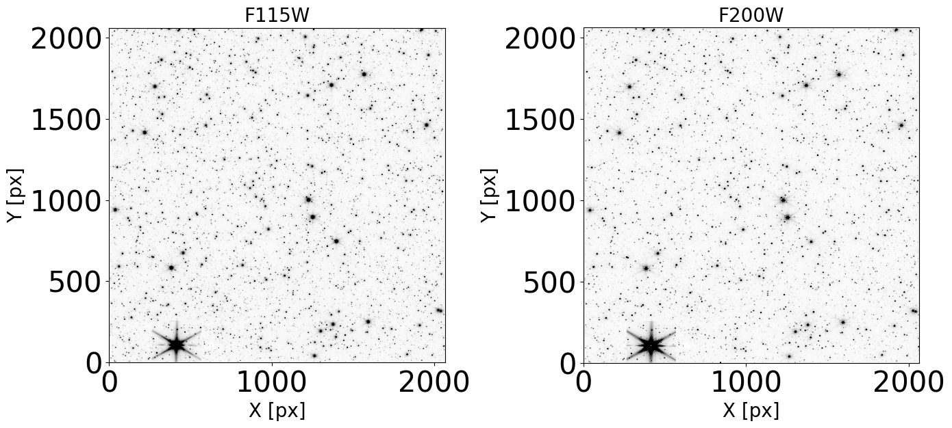
Data: NIRCam simulated images obtained using MIRAGE and run through the JWST pipeline of the Large Magellanic Cloud (LMC) Astrometric Calibration Field. Simulations is obtained using a 4-pt subpixel dither for three couples of wide filters: F070W, F115W, and F200W for the SW channel, and F277W, F356W, and F444W for the LW channel. We simulated only 1 NIRCam SW detector (i.e., “NRCB1”). For this example, we use Level-3 images (calibrated and rectified) for two SW filters (i.e., F115W and F200W) and derive the aperture photometry in each one of them. The images for the other filters are also available and can be used to test the notebook and/or different filters combination.
Tools: astropy, photutils.
Cross-intrument: NIRSpec, NIRISS, MIRI.
Documentation: This notebook is part of a STScI’s larger post-pipeline Data Analysis Tools Ecosystem.

Final plots show:

Instrumental Color-Magnitude Diagrams and errors
Magnitudes Zeropoints
Calibrated Color-Magnitude Diagram (compared with Input Color-Magnitude Diagram)
Comparison between input and output photometry

Import Functions#

import os
import sys
import time

import numpy as np

import pandas as pd

import glob as glob

import tarfile

import urllib.request

import jwst
from jwst.datamodels import ImageModel

from astropy.io import fits
from astropy.table import Table
from astropy.visualization import (ZScaleInterval, SqrtStretch, ImageNormalize)
from astropy.visualization import simple_norm
from astropy.stats import sigma_clipped_stats, SigmaClip
from astropy.coordinates import SkyCoord, match_coordinates_sky
from astropy import units as u

from photutils.detection import DAOStarFinder
from photutils.background import MMMBackground, MADStdBackgroundRMS, Background2D
from photutils.aperture import CircularAperture, CircularAnnulus, aperture_photometry

Import Plotting Functions#

%matplotlib inline
from matplotlib import style, pyplot as plt
import matplotlib.patches as patches
import matplotlib.ticker as ticker

plt.rcParams['image.cmap'] = 'viridis'
plt.rcParams['image.origin'] = 'lower'
plt.rcParams['axes.titlesize'] = plt.rcParams['axes.labelsize'] = 30
plt.rcParams['xtick.labelsize'] = plt.rcParams['ytick.labelsize'] = 30

font1 = {'family': 'helvetica', 'color': 'black', 'weight': 'normal', 'size': '12'}
font2 = {'family': 'helvetica', 'color': 'black', 'weight': 'normal', 'size': '20'}

Load Images and create some useful dictionaries#

We load all the images and we create a dictionary that contains all of them, divided by detectors and filters. This is useful to check which detectors and filters are available and to decide if we want to perform the photometry on all of them or only on a subset (for example, only on the SW filters).

We also create a dictionary with some useful parameters for the analysis. The dictionary contains the photometric zeropoints (from MIRAGE configuration files) and the NIRCam point spread function (PSF) FWHM, from the NIRCam Point Spread Function JDox page. The FWHM are calculated from the analysis of the expected NIRCam PSFs simulated with WebbPSF.

Note: this dictionary will be updated once the values for zeropoints and FWHM will be available for each detectors/filters after commissioning.

Hence, we have two dictionaries:

dictionary for the Level-3 images
dictionary with some other useful parameters

dict_images = {'NRCA1': {}, 'NRCA2': {}, 'NRCA3': {}, 'NRCA4': {}, 'NRCA5': {},
               'NRCB1': {}, 'NRCB2': {}, 'NRCB3': {}, 'NRCB4': {}, 'NRCB5': {}}

dict_filter_short = {}
dict_filter_long = {}

ff_short = []
det_short = []
det_long = []
ff_long = []
detlist_short = []
detlist_long = []
filtlist_short = []
filtlist_long = []

if not glob.glob('./*combined*fits'):

    print("Downloading images")

    boxlink_images_lev3 = 'https://data.science.stsci.edu/redirect/JWST/jwst-data_analysis_tools/stellar_photometry/images_level3.tar.gz'
    boxfile_images_lev3 = './images_level3.tar.gz'
    urllib.request.urlretrieve(boxlink_images_lev3, boxfile_images_lev3)

    tar = tarfile.open(boxfile_images_lev3, 'r')
    tar.extractall()

    images_dir = './'
    images = sorted(glob.glob(os.path.join(images_dir, "*combined*fits")))

else:

    images_dir = './'
    images = sorted(glob.glob(os.path.join(images_dir, "*combined*fits")))

for image in images:

    im = fits.open(image)
    f = im[0].header['FILTER']
    d = im[0].header['DETECTOR']

    if d == 'NRCBLONG':
        d = 'NRCB5'
    elif d == 'NRCALONG':
        d = 'NRCA5'
    else:
        d = d

    wv = float(f[1:3])

    if wv > 24:
        ff_long.append(f)
        det_long.append(d)

    else:
        ff_short.append(f)
        det_short.append(d)

    detlist_short = sorted(list(dict.fromkeys(det_short)))
    detlist_long = sorted(list(dict.fromkeys(det_long)))

    unique_list_filters_short = []
    unique_list_filters_long = []

    for x in ff_short:

        if x not in unique_list_filters_short:

            dict_filter_short.setdefault(x, {})

    for x in ff_long:
        if x not in unique_list_filters_long:
            dict_filter_long.setdefault(x, {})

    for d_s in detlist_short:
        dict_images[d_s] = dict_filter_short

    for d_l in detlist_long:
        dict_images[d_l] = dict_filter_long

    filtlist_short = sorted(list(dict.fromkeys(dict_filter_short)))
    filtlist_long = sorted(list(dict.fromkeys(dict_filter_long)))

    if len(dict_images[d][f]) == 0:
        dict_images[d][f] = {'images': [image]}
    else:
        dict_images[d][f]['images'].append(image)

print("Available Detectors for SW channel:", detlist_short)
print("Available Detectors for LW channel:", detlist_long)
print("Available SW Filters:", filtlist_short)
print("Available LW Filters:", filtlist_long)

Downloading images
Available Detectors for SW channel: ['NRCB1']
Available Detectors for LW channel: ['NRCB5']
Available SW Filters: ['F070W', 'F115W', 'F200W']
Available LW Filters: ['F277W', 'F356W', 'F444W']

filters = ['F070W', 'F090W', 'F115W', 'F140M', 'F150W2', 'F150W', 'F162M', 'F164N', 'F182M',
           'F187N', 'F200W', 'F210M', 'F212N', 'F250M', 'F277W', 'F300M', 'F322W2', 'F323N',
           'F335M', 'F356W', 'F360M', 'F405N', 'F410M', 'F430M', 'F444W', 'F460M', 'F466N', 'F470N', 'F480M']

psf_fwhm = [0.987, 1.103, 1.298, 1.553, 1.628, 1.770, 1.801, 1.494, 1.990, 2.060, 2.141, 2.304, 2.341, 1.340,
            1.444, 1.585, 1.547, 1.711, 1.760, 1.830, 1.901, 2.165, 2.179, 2.300, 2.302, 2.459, 2.507, 2.535, 2.574]

zp_modA = [25.7977, 25.9686, 25.8419, 24.8878, 27.0048, 25.6536, 24.6957, 22.3073, 24.8258, 22.1775, 25.3677, 24.3296,
           22.1036, 22.7850, 23.5964, 24.8239, 23.6452, 25.3648, 20.8604, 23.5873, 24.3778, 23.4778, 20.5588,
           23.2749, 22.3584, 23.9731, 21.9502, 20.0428, 19.8869, 21.9002]

zp_modB = [25.7568, 25.9771, 25.8041, 24.8738, 26.9821, 25.6279, 24.6767, 22.2903, 24.8042, 22.1499, 25.3391, 24.2909,
           22.0574, 22.7596, 23.5011, 24.6792, 23.5769, 25.3455, 20.8631, 23.4885, 24.3883, 23.4555, 20.7007,
           23.2763, 22.4677, 24.1562, 22.0422, 20.1430, 20.0173, 22.4086]

dict_utils = {filters[i]: {'psf fwhm': psf_fwhm[i], 'VegaMAG zp modA': zp_modA[i],
                           'VegaMAG zp modB': zp_modB[i]} for i in range(len(filters))}

Select the detectors and/or filters for the analysis#

If we are interested only in some filters (and/or some detectors) in the analysis, as in this example, we can select the images from the dictionary for those filters (detectors) and analyze only those images.

In this particular example, we analyze images for filters F115W and F200W for the detector NRCB1.

dets_short = ['NRCB1']  # detector of interest in this example
filts_short = ['F115W', 'F200W']  # filters of interest in this example

Display the images#

To check that our images do not present artifacts and can be used in the analysis, we display them.

plt.figure(figsize=(14, 14))

for det in dets_short:
    for i, filt in enumerate(filts_short):

        image = fits.open(dict_images[det][filt]['images'][0])
        data_sb = image[1].data

        ax = plt.subplot(1, len(filts_short), i + 1)

        plt.xlabel("X [px]", fontdict=font2)
        plt.ylabel("Y [px]", fontdict=font2)
        plt.title(filt, fontdict=font2)
        norm = simple_norm(data_sb, 'sqrt', percent=99.)

        ax.imshow(data_sb, norm=norm, cmap='Greys')

plt.tight_layout()

findfont: Font family 'helvetica' not found.
findfont: Font family 'helvetica' not found.
findfont: Font family 'helvetica' not found.
findfont: Font family 'helvetica' not found.
findfont: Font family 'helvetica' not found.
findfont: Font family 'helvetica' not found.
findfont: Font family 'helvetica' not found.
findfont: Font family 'helvetica' not found.
findfont: Font family 'helvetica' not found.
findfont: Font family 'helvetica' not found.
findfont: Font family 'helvetica' not found.
findfont: Font family 'helvetica' not found.
findfont: Font family 'helvetica' not found.
findfont: Font family 'helvetica' not found.
findfont: Font family 'helvetica' not found.
findfont: Font family 'helvetica' not found.
findfont: Font family 'helvetica' not found.
findfont: Font family 'helvetica' not found.
findfont: Font family 'helvetica' not found.
findfont: Font family 'helvetica' not found.
findfont: Font family 'helvetica' not found.
findfont: Font family 'helvetica' not found.

../../_images/700f0f8d9906ca08a39f1a404375478f1f86985f7901a9d989547c81f5bd78c1.png

Aperture Photometry#

More information on aperture photometry using Photutils can be found here: Aperture Photometry

First, we create a useful dictionary that contains: the sources detected using our finding algorithm (DAOStarFinder), the table with the aperture photometry results, and a final table with positions (both x,y and RA,Dec) instrumental magnitudes ad errors for the detected sources.

dict_aper = {}

for det in dets_short:
    dict_aper.setdefault(det, {})
    for j, filt in enumerate(filts_short):
        dict_aper[det].setdefault(filt, {})

        dict_aper[det][filt]['sources found'] = None
        dict_aper[det][filt]['aperture phot table'] = None
        dict_aper[det][filt]['final aperture phot table'] = None

1. Finding sources#

DAOStarFinder detects stars in an image using the DAOFIND (Stetson 1987) algorithm. DAOFIND searches images for local density maxima that have a peak amplitude greater than threshold (approximately; threshold is applied to a convolved image) and have a size and shape similar to the defined 2D Gaussian kernel.

Note: we adopted as Background estimator the function MMMBackground, which calculates the background in an array using the DAOPHOT MMM algorithm, on the whole image.

When dealing with a variable background and/or the need to mask the regions where we have no data (for example, if we are analyzing an image with all the 4 NIRCam SW detectors, i.e. containing the chip gaps), we can set var_bkg = True and use a more complex algorithm that takes into account those issues.

Note that the unit of the Level-2 and Level-3 Images from the pipeline is MJy/sr (hence a surface brightness). The actual unit of the image can be checked from the header keyword BUNIT. The scalar conversion constant is copied to the header keyword PHOTMJSR, which gives the conversion from DN/s to megaJy/steradian. For our analysis we revert back to DN/s.

def find_stars(det='NRCA1', filt='F070W', var_bkg=False):

    bkgrms = MADStdBackgroundRMS()
    mmm_bkg = MMMBackground()

    image = fits.open(dict_images[det][filt]['images'][i])
    data_sb = image[1].data
    imh = image[1].header

    print("Finding sources on image {number}, filter {f}, detector {d}:".format(number=i + 1, f=filt, d=det))
    print("")
    data = data_sb / imh['PHOTMJSR']
    print("Conversion factor from {units} to DN/S for filter {f}:".format(units=imh['BUNIT'], f=filt), imh['PHOTMJSR'])

    sigma_psf = dict_utils[filt]['psf fwhm']

    print("FWHM for the filter {f}:".format(f=filt), sigma_psf, "px")

    if var_bkg:
        print("Using 2D Background")
        sigma_clip = SigmaClip(sigma=3.)
        coverage_mask = (data == 0)

        bkg = Background2D(data, (25, 25), filter_size=(3, 3), sigma_clip=sigma_clip, bkg_estimator=mmm_bkg,
                           coverage_mask=coverage_mask, fill_value=0.0)

        data_bkgsub = data.copy()
        data_bkgsub = data_bkgsub - bkg.background

        _, _, std = sigma_clipped_stats(data_bkgsub)

    else:

        std = bkgrms(data)
        bkg = mmm_bkg(data)

        data_bkgsub = data.copy()
        data_bkgsub -= bkg

    daofind = DAOStarFinder(threshold=th[j] * std, fwhm=sigma_psf, roundhi=1.0,
                            roundlo=-1.0, sharplo=0.30, sharphi=1.40)

    found_stars = daofind(data_bkgsub)
    dict_aper[det][filt]['sources found'] = found_stars
    print("")
    print("Number of sources found in the image:", len(found_stars))
    print("-------------------------------------")
    print("")

tic = time.perf_counter()

th = [10, 10]  # threshold level for the two filters (length must match number of filters analyzed)

for det in dets_short:
    for j, filt in enumerate(filts_short):
        for i in np.arange(0, len(dict_images[det][filt]['images']), 1):

            find_stars(det=det, filt=filt, var_bkg=False)

toc = time.perf_counter()

print("Elapsed Time for finding stars:", toc - tic)

Finding sources on image 1, filter F115W, detector NRCB1:

Conversion factor from MJy/sr to DN/S for filter F115W: 3.821892261505127
FWHM for the filter F115W: 1.298 px

Number of sources found in the image: 11034
-------------------------------------

Finding sources on image 1, filter F200W, detector NRCB1:

Conversion factor from MJy/sr to DN/S for filter F200W: 2.564082860946655
FWHM for the filter F200W: 2.141 px

Number of sources found in the image: 12013
-------------------------------------

Elapsed Time for finding stars: 4.087729034999995

2. Aperture Photometry#

In the function below that allows to perform aperture photometry, we need to specify 4 parameters: the filter (i.e., image) used in the analysis, the aperture radius and the inner and outer radii for the annulus used to determine the local background. Values for the aperture radius and the annulii depend on the adopted filter and the user science case.

Note that Aperture object support multiple positions, allowing to perform photometry in multiple apertures at each position. For multiple apertures, the output table column names are appended with the positions index.

def aperture_phot(det=det, filt=filt, radius=[3.5], sky_in=7, sky_out=10):

    positions = np.transpose((dict_aper[det][filt]['sources found']['xcentroid'],
                              dict_aper[det][filt]['sources found']['ycentroid']))

    image = fits.open(dict_images[det][filt]['images'][0])
    data_sb = image[1].data
    imh = image[1].header
    data = data_sb / imh['PHOTMJSR']
    aa = np.argwhere(data < 0)

    for i in np.arange(0, len(aa), 1):
        data[aa[i][0], aa[i][1]] = 0

    error = np.sqrt(data)

    tic = time.perf_counter()

    table_aper = Table()

    for rad in radius:
        print("Performing aperture photometry for filter {1}; radius r = {0} px".format(rad, filt))
        rr = str(rad)
        aperture = CircularAperture(positions, r=rad)
        annulus_aperture = CircularAnnulus(positions, r_in=sky_in, r_out=sky_out)
        annulus_mask = annulus_aperture.to_mask(method='center')

        bkg_median = []
        bkg_stdev = []
        for mask in annulus_mask:
            annulus_data = mask.multiply(data)
            annulus_data_1d = annulus_data[mask.data > 0]
            _, median_sigclip, stdev_sigclip = sigma_clipped_stats(annulus_data_1d)
            bkg_median.append(median_sigclip)
            bkg_stdev.append(stdev_sigclip)
        bkg_median = np.array(bkg_median)
        bkg_stdev = np.array(bkg_stdev)

        phot = aperture_photometry(data, aperture, method='exact', error=error)

        phot['annulus_median'] = bkg_median
        phot['aper_bkg'] = bkg_median * aperture.area
        phot['aper_sum_bkgsub'] = phot['aperture_sum'] - phot['aper_bkg']

        table_aper.add_column(phot['aperture_sum'], name='aper_sum_' + rr + 'px')
        table_aper.add_column(phot['annulus_median'], name='annulus_median_' + rr + 'px')
        table_aper.add_column(phot['aper_bkg'], name='aper_bkg_' + rr + 'px')
        table_aper.add_column(phot['aper_sum_bkgsub'], name='aper_sum_bkgsub_' + rr + 'px')

        error_poisson = phot['aperture_sum_err']
        error_scatter_sky = aperture.area * bkg_stdev**2
        error_mean_sky = bkg_stdev**2 * aperture.area**2 / annulus_aperture.area

        fluxerr = np.sqrt(error_poisson + error_scatter_sky + error_mean_sky)

        table_aper.add_column(fluxerr, name='flux_err_' + rr + 'px')

        dict_aper[det][filt]['aperture phot table'] = table_aper

    toc = time.perf_counter()
    print("Time Elapsed:", toc - tic)

    return

det = 'NRCB1'
filt1 = 'F115W'
filt2 = 'F200W'

aperture_phot(det=det, filt=filt1, radius=[3.5], sky_in=7, sky_out=10)
aperture_phot(det=det, filt=filt2, radius=[4.0], sky_in=6, sky_out=9)

Performing aperture photometry for filter F115W; radius r = 3.5 px
Time Elapsed: 6.936824905999998
Performing aperture photometry for filter F200W; radius r = 4.0 px
Time Elapsed: 7.191780198999993

3. Table with magnitudes and positions#

We create the final tables containing positions, magnitudes and errors for each catalog

radii = [3.5, 4.0]

for det in dets_short:
    for j, filt in enumerate(filts_short):
        for i in np.arange(0, len(dict_images[det][filt]['images']), 1):

            radius = str(radii[j])

            image = fits.open(dict_images[det][filt]['images'][0])
            data = image[1].data

            image_model = ImageModel(dict_images[det][filt]['images'][0])

            mask = ((dict_aper[det][filt]['sources found']['xcentroid'] > 0) &
                    (dict_aper[det][filt]['sources found']['xcentroid'] < data.shape[1]) &
                    (dict_aper[det][filt]['sources found']['ycentroid'] > 0) &
                    (dict_aper[det][filt]['sources found']['ycentroid'] < data.shape[0]) &
                    (dict_aper[det][filt]['aperture phot table']['aper_sum_bkgsub_' + radius + 'px'] > 0))

            table_phot = Table()

            table_phot['x'] = dict_aper[det][filt]['sources found']['xcentroid'][mask]
            table_phot['y'] = dict_aper[det][filt]['sources found']['ycentroid'][mask]

            ra, dec = image_model.meta.wcs(table_phot['x'], table_phot['y'])
            table_phot['radec'] = SkyCoord(ra, dec, unit='deg')
            table_phot[filt + '_inst'] = -2.5 * np.log10(dict_aper[det][filt]['aperture phot table']['aper_sum_bkgsub_' + radius + 'px'][mask])
            table_phot['e' + filt + '_inst'] = 1.086 * (dict_aper[det][filt]['aperture phot table']['flux_err_' + radius + 'px'][mask] /
                                                        dict_aper[det][filt]['aperture phot table']['aper_sum_bkgsub_' + radius + 'px'][mask])

            dict_aper[det][filt]['final aperture phot table'] = table_phot

Matched sources Table#

We cross-match the catalogs to obtain the single color-magnitude diagram.

Stars from the two filters are associated if the distance between the matches is < 0.5 px.

max_sep = 0.015 * u.arcsec

idx_inst, d2d_inst, _ = match_coordinates_sky(dict_aper[det][filt1]['final aperture phot table']['radec'],
                                              dict_aper[det][filt2]['final aperture phot table']['radec'])

sep_constraint_inst = d2d_inst < max_sep

matched_sources = Table()

matched_sources['radec'] = dict_aper[det][filt1]['final aperture phot table']['radec'][sep_constraint_inst]
matched_sources['x_' + filt1] = dict_aper[det][filt1]['final aperture phot table']['x'][sep_constraint_inst]
matched_sources['y_' + filt1] = dict_aper[det][filt1]['final aperture phot table']['y'][sep_constraint_inst]
matched_sources['x_' + filt2] = dict_aper[det][filt2]['final aperture phot table']['x'][idx_inst[sep_constraint_inst]]
matched_sources['y_' + filt2] = dict_aper[det][filt2]['final aperture phot table']['y'][idx_inst[sep_constraint_inst]]
matched_sources[filt1 + '_inst'] = dict_aper[det][filt1]['final aperture phot table'][filt1 + '_inst'][sep_constraint_inst]
matched_sources['e' + filt1 + '_inst'] = dict_aper[det][filt1]['final aperture phot table']['e' + filt1 + '_inst'][sep_constraint_inst]
matched_sources[filt2 + '_inst'] = dict_aper[det][filt2]['final aperture phot table'][filt2 + '_inst'][idx_inst[sep_constraint_inst]]
matched_sources['e' + filt2 + '_inst'] = dict_aper[det][filt2]['final aperture phot table']['e' + filt2 + '_inst'][idx_inst[sep_constraint_inst]]

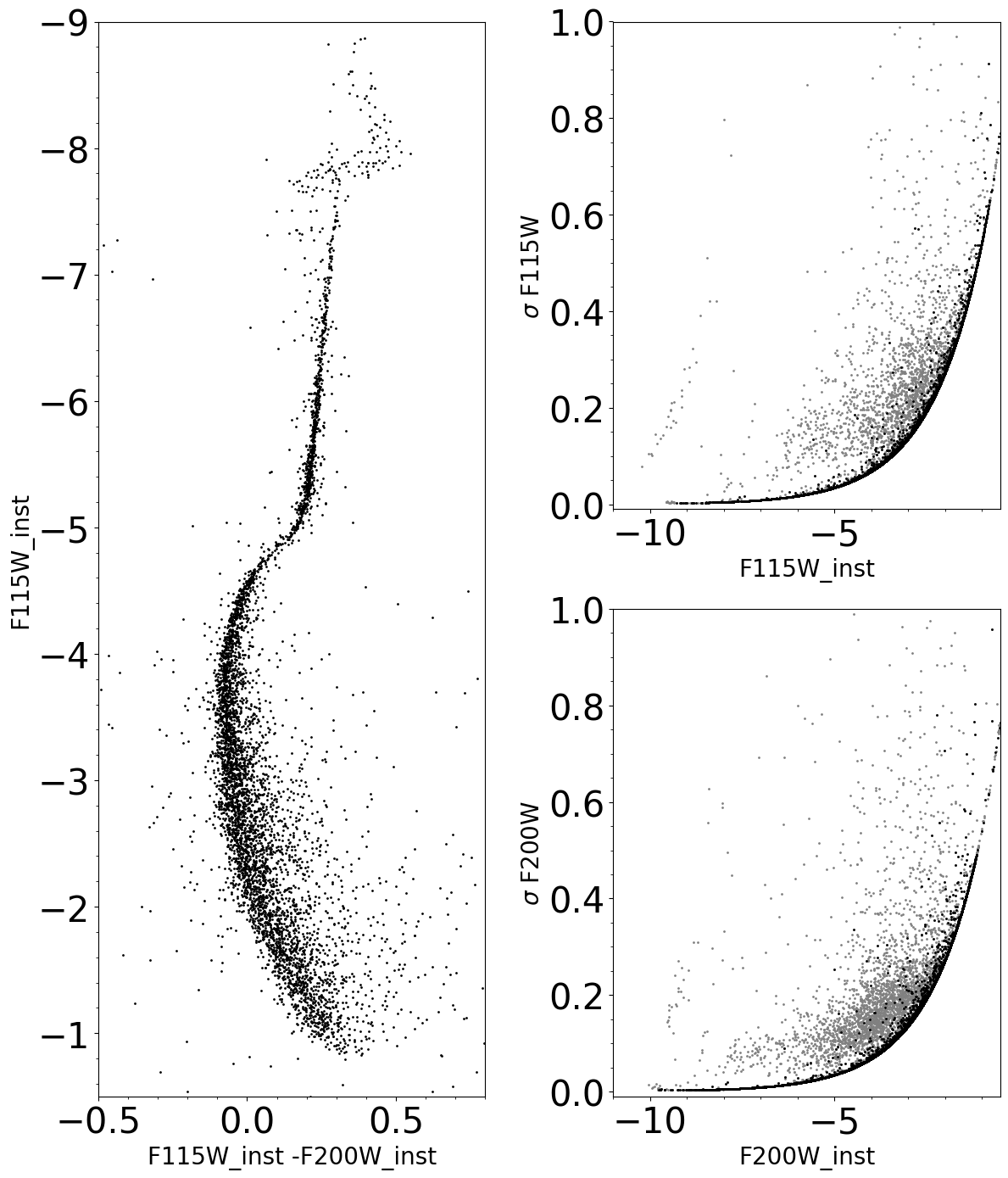
Instrumental Color-Magnitude Diagram and Errors#

In the error plots, the grey dots represent measures all the detections in each filter, whereas the black dots represent the detections matched between the two catalogs.

plt.figure(figsize=(12, 14))
plt.clf()

ax1 = plt.subplot(1, 2, 1)

ax1.set_xlabel(filt1 + '_inst -' + filt2 + '_inst', fontdict=font2)
ax1.set_ylabel(filt1 + '_inst', fontdict=font2)

xlim0 = -0.5
xlim1 = 0.8
ylim0 = -0.5
ylim1 = -9

ax1.set_xlim(xlim0, xlim1)
ax1.set_ylim(ylim0, ylim1)

ax1.xaxis.set_major_locator(ticker.AutoLocator())
ax1.xaxis.set_minor_locator(ticker.AutoMinorLocator())
ax1.yaxis.set_major_locator(ticker.AutoLocator())
ax1.yaxis.set_minor_locator(ticker.AutoMinorLocator())

ax1.scatter(matched_sources[filt1 + '_inst'] - matched_sources[filt2 + '_inst'], matched_sources[filt1 + '_inst'],
            s=1, color='k')

ax2 = plt.subplot(2, 2, 2)

ax2.set_xlabel(filt1 + '_inst', fontdict=font2)
ax2.set_ylabel('$\sigma$ ' + filt1, fontdict=font2)

xlim0 = -11
xlim1 = -0.5
ylim0 = -0.01
ylim1 = 1

ax2.set_xlim(xlim0, xlim1)
ax2.set_ylim(ylim0, ylim1)

ax2.xaxis.set_major_locator(ticker.AutoLocator())
ax2.xaxis.set_minor_locator(ticker.AutoMinorLocator())
ax2.yaxis.set_major_locator(ticker.AutoLocator())
ax2.yaxis.set_minor_locator(ticker.AutoMinorLocator())

ax2.scatter(dict_aper[det][filt1]['final aperture phot table'][filt1 + '_inst'],
            dict_aper[det][filt1]['final aperture phot table']['e' + filt1 + '_inst'], s=1, c='gray')

ax2.scatter(matched_sources[filt1 + '_inst'], matched_sources['e' + filt1 + '_inst'], s=1, c='k')

ax3 = plt.subplot(2, 2, 4)

ax3.set_xlabel(filt2 + '_inst', fontdict=font2)
ax3.set_ylabel('$\sigma$ ' + filt2, fontdict=font2)

ax3.set_xlim(xlim0, xlim1)
ax3.set_ylim(ylim0, ylim1)

ax3.xaxis.set_major_locator(ticker.AutoLocator())
ax3.xaxis.set_minor_locator(ticker.AutoMinorLocator())
ax3.yaxis.set_major_locator(ticker.AutoLocator())
ax3.yaxis.set_minor_locator(ticker.AutoMinorLocator())

ax3.scatter(dict_aper[det][filt2]['final aperture phot table'][filt2 + '_inst'],
            dict_aper[det][filt2]['final aperture phot table']['e' + filt2 + '_inst'], s=1, c='gray')

ax3.scatter(matched_sources[filt2 + '_inst'], matched_sources['e' + filt2 + '_inst'], s=1, c='k')

plt.tight_layout()

2023-12-13 15:08:44,677 - stpipe - WARNING - findfont: Font family 'helvetica' not found.
2023-12-13 15:08:44,679 - stpipe - WARNING - findfont: Font family 'helvetica' not found.
2023-12-13 15:08:44,726 - stpipe - WARNING - findfont: Font family 'helvetica' not found.
2023-12-13 15:08:44,773 - stpipe - WARNING - findfont: Font family ['helvetica'] not found. Falling back to DejaVu Sans.
2023-12-13 15:08:44,850 - stpipe - WARNING - findfont: Font family 'helvetica' not found.
2023-12-13 15:08:44,890 - stpipe - WARNING - findfont: Font family 'helvetica' not found.
2023-12-13 15:08:44,906 - stpipe - WARNING - findfont: Font family 'helvetica' not found.
2023-12-13 15:08:44,925 - stpipe - WARNING - findfont: Font family 'helvetica' not found.
2023-12-13 15:08:44,954 - stpipe - WARNING - findfont: Font family 'helvetica' not found.
2023-12-13 15:08:45,135 - stpipe - WARNING - findfont: Font family 'helvetica' not found.
2023-12-13 15:08:45,136 - stpipe - WARNING - findfont: Font family 'helvetica' not found.
2023-12-13 15:08:45,137 - stpipe - WARNING - findfont: Font family 'helvetica' not found.
2023-12-13 15:08:45,154 - stpipe - WARNING - findfont: Font family 'helvetica' not found.
2023-12-13 15:08:45,155 - stpipe - WARNING - findfont: Font family 'helvetica' not found.
2023-12-13 15:08:45,175 - stpipe - WARNING - findfont: Font family 'helvetica' not found.
2023-12-13 15:08:45,206 - stpipe - WARNING - findfont: Font family 'helvetica' not found.
2023-12-13 15:08:45,207 - stpipe - WARNING - findfont: Font family 'helvetica' not found.

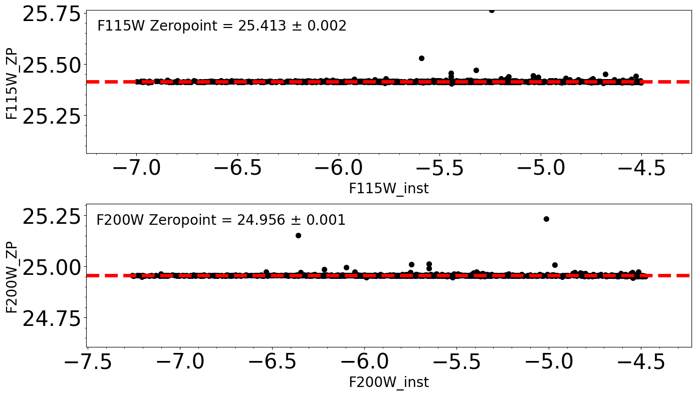
../../_images/37ecb55aaf699864142a0e0a566f99671abf4c09c45e6ecce339e8ce4584da44.png

Photometric Zeropoints#

To obtain the final calibrated color-magnitude diagram, we need to calculate the photometric zeropoints. Hence we need to perform aperture photometry on the images using an aperture radius correspondent to a value of the encircled energy (EE), apply the appropriate aperture correction for the finite aperture adopted (the values provided in the dictionary above are for an infinite aperture) and then compare it with the aperture photometry determined above. Hence, we can summarize the steps as follows:

perform aperture photometry using an appropriate radius (equivalent to a certain value of the EE)
apply appropriate aperture correction
apply tabulated zeropoint
cross-match with aperture photometry

Note: to select the stars for the zeropoint calculation, we can select a subsample using the CMD as a reference, or perform aperture photometry on a sample of bright isolated stars. To change the method used we can set sample = cmd or sample = found, respectively.

Load aperture correction table#

Note: these values are obtained from the study of the synthetic WebbPSF PSFs. They will be updated once we have in-flight measures.

if os.path.isfile('./aperture_correction_table.txt'):
    ap_tab = './aperture_correction_table.txt'
else:
    print("Downloading the aperture correction table")

    boxlink_apcorr_table = 'https://data.science.stsci.edu/redirect/JWST/jwst-data_analysis_tools/stellar_photometry/aperture_correction_table.txt'
    boxfile_apcorr_table = './aperture_correction_table.txt'
    urllib.request.urlretrieve(boxlink_apcorr_table, boxfile_apcorr_table)
    ap_tab = './aperture_correction_table.txt'

aper_table = pd.read_csv(ap_tab, header=None, sep='\s+', index_col=0,
                         names=['filter', 'pupil', 'wave', 'r10', 'r20', 'r30', 'r40', 'r50', 'r60', 'r70', 'r80',
                                'r85', 'r90', 'sky_flux_px', 'apcorr10', 'apcorr20', 'apcorr30', 'apcorr40',
                                'apcorr50', 'apcorr60', 'apcorr70', 'apcorr80', 'apcorr85', 'apcorr90', 'sky_in',
                                'sky_out'], comment='#', skiprows=0, usecols=range(0, 26))
aper_table.head()

Downloading the aperture correction table

	pupil	wave	r10	r20	r30	r40	r50	r60	r70	r80	...	apcorr30	apcorr40	apcorr50	apcorr60	apcorr70	apcorr80	apcorr85	apcorr90	sky_in	sky_out
filter
F070W	CLEAR	70	0.451	0.869	1.263	1.648	2.191	3.266	5.176	7.292	...	3.3651	2.5305	2.0347	1.7210	1.5328	1.4174	1.4174	1.5880	7.292	9.017
F090W	CLEAR	90	0.408	0.638	0.992	1.503	1.925	2.549	4.162	7.480	...	3.3519	2.5241	2.0253	1.6977	1.4908	1.4173	1.4173	1.6016	7.480	9.251
F115W	CLEAR	115	0.374	0.571	0.778	1.036	1.768	2.324	3.287	6.829	...	3.3404	2.5070	2.0131	1.6825	1.4520	1.3310	1.3310	1.3964	6.829	9.723
F140M	CLEAR	140	0.414	0.617	0.801	1.031	1.367	2.434	3.118	6.031	...	3.3397	2.5060	2.0067	1.6815	1.4465	1.3029	1.3029	1.3794	6.031	9.608
F150W	CLEAR	150	0.431	0.639	0.826	1.065	1.360	2.476	3.199	6.082	...	3.3405	2.5067	2.0070	1.6828	1.4485	1.3068	1.3068	1.4188	6.082	9.496

5 rows × 25 columns

1a. Subsample using the CMD as a reference#

Note: if the users want to impose a more stringent condition, selecting within the sub-sample of stars the ones with no neighbour closer than X pixel, where X can be fixed appropriately, it can be done setting dist_sel = True.

The limiting magnitudes and the maximum distance to the closest neighbour depend on the user science case (i.e.; number of stars in the field of view, crowding, number of bright sources, etc.) and must be modified accordingly.

The final table xy_cmd contain the positions (X,Y) of the selected stars in the two filters.

xy_cmd = Table()

mag_lim_bright = -7.0
mag_lim_faint = -4.5

mask_xy = ((matched_sources[filt1 + '_inst'] < mag_lim_faint) & (matched_sources[filt1 + '_inst'] > mag_lim_bright))

xy_cmd['x_' + filt1] = matched_sources['x_' + filt1][mask_xy]
xy_cmd['y_' + filt1] = matched_sources['y_' + filt1][mask_xy]
xy_cmd['x_' + filt2] = matched_sources['x_' + filt2][mask_xy]
xy_cmd['y_' + filt2] = matched_sources['y_' + filt2][mask_xy]

print("Number of stars selected from CMD:", len(xy_cmd))

dist_sel = False

if dist_sel:

    print("")
    print("Calculating closest neigbhour distance")

    d_filt1 = []
    d_filt2 = []
    min_sep_filt1 = 10
    min_sep_filt2 = 10

    for i, j in zip(xy_cmd['x_' + filt1], xy_cmd['y_' + filt1]):

        sep = []
        dist = np.sqrt((dict_aper[det][filt1]['sources found']['xcentroid'] - i)**2 + (dict_aper[det][filt1]['sources found']['ycentroid'] - j)**2)
        sep = np.sort(dist)[1:2][0]
        d_filt1.append(sep)

    for i, j in zip(xy_cmd['x_' + filt2], xy_cmd['y_' + filt2]):

        sep = []
        dist = np.sqrt((dict_aper[det][filt2]['sources found']['xcentroid'] - i)**2 + (dict_aper[det][filt2]['sources found']['ycentroid'] - j)**2)
        sep = np.sort(dist)[1:2][0]
        d_filt2.append(sep)

    xy_cmd['min distance ' + filt1] = d_filt1
    xy_cmd['min distance ' + filt2] = d_filt2

    mask_dist = ((xy_cmd['min distance ' + filt1] > min_sep_filt1) & (xy_cmd['min distance ' + filt2] > min_sep_filt2))

    xy_cmd = xy_cmd[mask_dist]

    print("")
    print("Minimum distance required for filter {f}:".format(f=filt1), min_sep_filt1, "px")
    print("Minimum distance required for filter {f}:".format(f=filt2), min_sep_filt2, "px")
    print("")
    print("Number of stars selected from CMD including distance constraints:", len(xy_cmd))

Number of stars selected from CMD: 896

As we have done previously, we create a dictionary that contains the tables with the derived aperture photometry (for the bright stars) for each image.

dict_zp = {}

for det in dets_short:
    dict_zp.setdefault(det, {})
    for j, filt in enumerate(filts_short):

        dict_zp[det].setdefault(filt, {})

        dict_zp[det][filt]['sources found'] = None
        dict_zp[det][filt]['aperture phot table'] = None
        dict_zp[det][filt]['final aperture phot table'] = None

def find_bright_stars(det='NRCA1', filt='F070W', var_bkg=False, dist_sel=False):

    bkgrms = MADStdBackgroundRMS()
    mmm_bkg = MMMBackground()

    image = fits.open(dict_images[det][filt]['images'][i])
    data_sb = image[1].data
    imh = image[1].header

    print("Finding sources on image {number}, filter {f}, detector {d}:".format(number=i + 1, f=filt, d=det))
    print("")
    data = data_sb / imh['PHOTMJSR']
    print("Conversion factor from {units} to DN/s for filter {f}:".format(units=imh['BUNIT'], f=filt), imh['PHOTMJSR'])

    sigma_psf = dict_utils[filt]['psf fwhm']

    print("FWHM for the filter {f}:".format(f=filt), sigma_psf, "px")

    if var_bkg:
        print("Using 2D Background")
        sigma_clip = SigmaClip(sigma=3.)
        coverage_mask = (data == 0)

        bkg = Background2D(data, (25, 25), filter_size=(3, 3), sigma_clip=sigma_clip,
                           bkg_estimator=mmm_bkg, coverage_mask=coverage_mask, fill_value=0.0)

        data_bkgsub = data.copy()
        data_bkgsub = data_bkgsub - bkg.background

        _, _, std = sigma_clipped_stats(data_bkgsub)

    else:

        std = bkgrms(data)
        bkg = mmm_bkg(data)

        data_bkgsub = data.copy()
        data_bkgsub -= bkg

    daofind = DAOStarFinder(threshold=th[j] * std, fwhm=sigma_psf, roundhi=1.0, roundlo=-1.0,
                            sharplo=0.30, sharphi=1.40)

    zp_stars = daofind(data_bkgsub)

    dict_zp[det][filt]['sources found'] = zp_stars

    if dist_sel:

        print("")
        print("Calculating closest neigbhour distance")

        d = []

        for xx, yy in zip(zp_stars['xcentroid'], zp_stars['ycentroid']):

            sep = []
            dist = np.sqrt((dict_aper[det][filt]['sources found']['xcentroid'] - xx)**2 +
                           (dict_aper[det][filt]['sources found']['ycentroid'] - yy)**2)
            sep = np.sort(dist)[1:2][0]
            d.append(sep)

        zp_stars['min distance'] = d
        mask_dist = (zp_stars['min distance'] > min_sep[j])

        zp_stars = zp_stars[mask_dist]

        dict_zp[det][filt]['sources found'] = zp_stars

        print("Minimum distance required:", min_sep[j], "px")
        print("")
        print("Number of bright isolated sources found in the image:", len(zp_stars))
        print("-----------------------------------------------------")
        print("")
    else:
        print("")
        print("Number of bright sources found in the image:", len(zp_stars))
        print("--------------------------------------------")
        print("")

The threshold and the maximum distance to the closest neighbour depend on the user science case (i.e.; number of stars in the field of view, crowding, number of bright sources, etc.) and must be modified accordingly.

tic = time.perf_counter()

th = [700, 500]  # threshold level for the two filters (length must match number of filters analyzed)
min_sep = [10, 10]  # minimum separation acceptable for zp stars from closest neighbour

for det in dets_short:
    for j, filt in enumerate(filts_short):
        for i in np.arange(0, len(dict_images[det][filt]['images']), 1):

            find_bright_stars(det=det, filt=filt, var_bkg=False, dist_sel=False)

toc = time.perf_counter()

print("Elapsed Time for finding stars:", toc - tic)

Finding sources on image 1, filter F115W, detector NRCB1:

Conversion factor from MJy/sr to DN/s for filter F115W: 3.821892261505127
FWHM for the filter F115W: 1.298 px

Number of bright sources found in the image: 1299
--------------------------------------------

Finding sources on image 1, filter F200W, detector NRCB1:

Conversion factor from MJy/sr to DN/s for filter F200W: 2.564082860946655
FWHM for the filter F200W: 2.141 px

Number of bright sources found in the image: 1479
--------------------------------------------

Elapsed Time for finding stars: 2.4704307259999894

Aperture Photometry on the bright isolated stars#

To select the sample of stars that we want to use in the aperture photometry, modify the sample keyword, using cmd or found.

def aperture_phot_zp(det=det, filt=filt, sample='found'):

    radii = [aper_table.loc[filt]['r70']]

    ees = '70'.split()
    ee_radii = dict(zip(ees, radii))

    if sample == 'found':

        positions = np.transpose((dict_zp[det][filt]['sources found']['xcentroid'],
                                  dict_zp[det][filt]['sources found']['ycentroid']))

    if sample == 'cmd':

        positions = np.transpose((xy_cmd['x_' + filt], xy_cmd['y_' + filt]))

    image = fits.open(dict_images[det][filt]['images'][0])
    data_sb = image[1].data
    imh = image[1].header
    data = data_sb / imh['PHOTMJSR']
    aa = np.argwhere(data < 0)

    for i in np.arange(0, len(aa), 1):
        data[aa[i][0], aa[i][1]] = 0

    # sky from the aperture correction table:

    sky = {"sky_in": aper_table.loc[filt]['r80'], "sky_out": aper_table.loc[filt]['r85']}

    tic = time.perf_counter()

    table_zp = Table()

    for ee, radius in ee_radii.items():
        print("Performing aperture photometry for radius equivalent to EE = {0}% for filter {1}".format(ee, filt))
        aperture = CircularAperture(positions, r=radius)
        annulus_aperture = CircularAnnulus(positions, r_in=sky["sky_in"], r_out=sky["sky_out"])
        annulus_mask = annulus_aperture.to_mask(method='center')

        bkg_median = []
        for mask in annulus_mask:
            annulus_data = mask.multiply(data)
            annulus_data_1d = annulus_data[mask.data > 0]
            _, median_sigclip, _ = sigma_clipped_stats(annulus_data_1d)
            bkg_median.append(median_sigclip)
        bkg_median = np.array(bkg_median)

        phot = aperture_photometry(data, aperture, method='exact')
        phot['annulus_median'] = bkg_median
        phot['aper_bkg'] = bkg_median * aperture.area
        phot['aper_sum_bkgsub'] = phot['aperture_sum'] - phot['aper_bkg']

        apcorr = [aper_table.loc[filt]['apcorr70']]

        phot['aper_sum_corrected'] = phot['aper_sum_bkgsub'] * apcorr

        table_zp.add_column(phot['aperture_sum'], name='aper_sum_' + ee)
        table_zp.add_column(phot['annulus_median'], name='annulus_median_' + ee)
        table_zp.add_column(phot['aper_bkg'], name='aper_bkg_ee_' + ee)
        table_zp.add_column(phot['aper_sum_bkgsub'], name='aper_sum_bkgsub_' + ee)
        table_zp.add_column(phot['aper_sum_corrected'], name='aper_sum_corrected_' + ee + '_' + filt)

        dict_zp[det][filt]['aperture phot table'] = table_zp

    toc = time.perf_counter()
    print("Time Elapsed:", toc - tic)

    return

aperture_phot_zp(det=det, filt=filt1, sample='cmd')
aperture_phot_zp(det=det, filt=filt2, sample='cmd')

Performing aperture photometry for radius equivalent to EE = 70% for filter F115W
Time Elapsed: 0.5191285669999957
Performing aperture photometry for radius equivalent to EE = 70% for filter F200W
Time Elapsed: 0.4871039350000217

ee = '70'
sample = 'cmd'

for det in dets_short:
    for j, filt in enumerate(filts_short):
        for i in np.arange(0, len(dict_images[det][filt]['images']), 1):

            image = fits.open(dict_images[det][filt]['images'][0])
            data = image[1].data

            image_model = ImageModel(dict_images[det][filt]['images'][0])
            table_zp_mag = Table()

            if sample == 'found':

                mask = ((dict_zp[det][filt]['sources found']['xcentroid'] > 0) &
                        (dict_zp[det][filt]['sources found']['xcentroid'] < data.shape[1]) &
                        (dict_zp[det][filt]['sources found']['ycentroid'] > 0) &
                        (dict_zp[det][filt]['sources found']['ycentroid'] < data.shape[0]) &
                        (dict_zp[det][filt]['aperture phot table']['aper_sum_corrected_' + ee + '_' + filt] > 0))

                table_zp_mag['x'] = dict_zp[det][filt]['sources found']['xcentroid'][mask]
                table_zp_mag['y'] = dict_zp[det][filt]['sources found']['ycentroid'][mask]

                ra, dec = image_model.meta.wcs(table_zp_mag['x'], table_zp_mag['y'])
                table_zp_mag['radec'] = SkyCoord(ra, dec, unit='deg')
                table_zp_mag[filt + '_inst'] = -2.5 * np.log10(dict_zp[det][filt]['aperture phot table']['aper_sum_corrected_' + ee + '_' + filt][mask])
                table_zp_mag[filt + '_zp'] = table_zp_mag[filt + '_inst'] + dict_utils[filt]['VegaMAG zp modB']

                dict_zp[det][filt]['final aperture phot table'] = table_zp_mag

            if sample == 'cmd':

                mask = ((dict_zp[det][filt]['aperture phot table']['aper_sum_corrected_' + ee + '_' + filt] > 0))

                table_zp_mag['x'] = xy_cmd['x_' + filt][mask]
                table_zp_mag['y'] = xy_cmd['y_' + filt][mask]
                ra, dec = image_model.meta.wcs(table_zp_mag['x'], table_zp_mag['y'])
                table_zp_mag['radec'] = SkyCoord(ra, dec, unit='deg')

                table_zp_mag[filt + '_inst'] = -2.5 * np.log10(dict_zp[det][filt]['aperture phot table']['aper_sum_corrected_' + ee + '_' + filt][mask])
                table_zp_mag[filt + '_zp'] = table_zp_mag[filt + '_inst'] + dict_utils[filt]['VegaMAG zp modB']

                dict_zp[det][filt]['final aperture phot table'] = table_zp_mag

Derive Zeropoints#

plt.figure(figsize=(14, 8))
plt.clf()

ax1 = plt.subplot(2, 1, 1)

ax1.set_xlabel(filt1 + '_inst', fontdict=font2)
ax1.set_ylabel(filt1 + '_ZP', fontdict=font2)

idx_zp_1, d2d_zp_1, _ = match_coordinates_sky(dict_zp[det][filt1]['final aperture phot table']['radec'],
                                              dict_aper[det][filt1]['final aperture phot table']['radec'])

sep_constraint_zp_1 = d2d_zp_1 < max_sep

f115w_apZP_matched = np.array(dict_zp[det][filt1]['final aperture phot table'][filt1 + '_zp'][sep_constraint_zp_1])
f115w_ap_matched = np.array(dict_aper[det][filt1]['final aperture phot table'][filt1 + '_inst'][idx_zp_1[sep_constraint_zp_1]])

diff_f115w = f115w_apZP_matched - f115w_ap_matched
_, zp_f115w, zp_sigma_f115w = sigma_clipped_stats(diff_f115w)

xlim0 = np.min(f115w_ap_matched) - 0.25
xlim1 = np.max(f115w_ap_matched) + 0.25
ylim0 = np.mean(diff_f115w) - 0.35
ylim1 = np.mean(diff_f115w) + 0.35

ax1.set_xlim(xlim0, xlim1)
ax1.set_ylim(ylim0, ylim1)

ax1.xaxis.set_major_locator(ticker.AutoLocator())
ax1.xaxis.set_minor_locator(ticker.AutoMinorLocator())
ax1.yaxis.set_major_locator(ticker.AutoLocator())
ax1.yaxis.set_minor_locator(ticker.AutoMinorLocator())

ax1.scatter(f115w_ap_matched, diff_f115w, s=50, color='k')
ax1.plot([xlim0, xlim1], [zp_f115w, zp_f115w], color='r', lw=5, ls='--')
ax1.text(xlim0 + 0.05, ylim1 - 0.1, filt1 + ' Zeropoint = %5.3f $\pm $ %5.3f' % (zp_f115w, zp_sigma_f115w),
         color='k', fontdict=font2)

ax2 = plt.subplot(2, 1, 2)

ax2.set_xlabel(filt2 + '_inst', fontdict=font2)
ax2.set_ylabel(filt2 + '_ZP', fontdict=font2)

idx_zp_2, d2d_zp_2, _ = match_coordinates_sky(dict_zp[det][filt2]['final aperture phot table']['radec'],
                                              dict_aper[det][filt2]['final aperture phot table']['radec'])

sep_constraint_zp_2 = d2d_zp_2 < max_sep

f200w_apZP_matched = np.array(dict_zp[det][filt2]['final aperture phot table'][filt2 + '_zp'][sep_constraint_zp_2])
f200w_ap_matched = np.array(dict_aper[det][filt2]['final aperture phot table'][filt2 + '_inst'][idx_zp_2[sep_constraint_zp_2]])

diff_f200w = f200w_apZP_matched - f200w_ap_matched
_, zp_f200w, zp_sigma_f200w = sigma_clipped_stats(diff_f200w)

xlim0 = np.min(f200w_ap_matched) - 0.25
xlim1 = np.max(f200w_ap_matched) + 0.25
ylim0 = np.mean(diff_f200w) - 0.35 
ylim1 = np.mean(diff_f200w) + 0.35

ax2.set_xlim(xlim0, xlim1)
ax2.set_ylim(ylim0, ylim1)

ax2.xaxis.set_major_locator(ticker.AutoLocator())
ax2.xaxis.set_minor_locator(ticker.AutoMinorLocator())
ax2.yaxis.set_major_locator(ticker.AutoLocator())
ax2.yaxis.set_minor_locator(ticker.AutoMinorLocator())

ax2.scatter(f200w_ap_matched, diff_f200w, s=50, color='k')
ax2.plot([xlim0, xlim1], [zp_f200w, zp_f200w], color='r', lw=5, ls='--')
ax2.text(xlim0 + 0.05, ylim1 - 0.1, filt2 + ' Zeropoint = %5.3f $\pm$ %5.3f' % (zp_f200w, zp_sigma_f200w), 
         color='k', fontdict=font2)

plt.tight_layout()

2023-12-13 15:08:54,192 - stpipe - WARNING - findfont: Font family 'helvetica' not found.
2023-12-13 15:08:54,193 - stpipe - WARNING - findfont: Font family 'helvetica' not found.
2023-12-13 15:08:54,209 - stpipe - WARNING - findfont: Font family 'helvetica' not found.
2023-12-13 15:08:54,246 - stpipe - WARNING - findfont: Font family 'helvetica' not found.
2023-12-13 15:08:54,262 - stpipe - WARNING - findfont: Font family 'helvetica' not found.
2023-12-13 15:08:54,288 - stpipe - WARNING - findfont: Font family 'helvetica' not found.
2023-12-13 15:08:54,297 - stpipe - WARNING - findfont: Font family 'helvetica' not found.
2023-12-13 15:08:54,316 - stpipe - WARNING - findfont: Font family 'helvetica' not found.
2023-12-13 15:08:54,324 - stpipe - WARNING - findfont: Font family 'helvetica' not found.
2023-12-13 15:08:54,453 - stpipe - WARNING - findfont: Font family 'helvetica' not found.
2023-12-13 15:08:54,454 - stpipe - WARNING - findfont: Font family 'helvetica' not found.
2023-12-13 15:08:54,455 - stpipe - WARNING - findfont: Font family 'helvetica' not found.
2023-12-13 15:08:54,463 - stpipe - WARNING - findfont: Font family 'helvetica' not found.
2023-12-13 15:08:54,464 - stpipe - WARNING - findfont: Font family 'helvetica' not found.
2023-12-13 15:08:54,484 - stpipe - WARNING - findfont: Font family 'helvetica' not found.
2023-12-13 15:08:54,485 - stpipe - WARNING - findfont: Font family 'helvetica' not found.
2023-12-13 15:08:54,493 - stpipe - WARNING - findfont: Font family 'helvetica' not found.
2023-12-13 15:08:54,494 - stpipe - WARNING - findfont: Font family 'helvetica' not found.

../../_images/a9a3cec0b0fc65e29c5b4acef0c4a264e2e8ded44a28c72b6581a4cde2d56f23.png

Import Input catalog#

if os.path.isfile('./pointsource.cat'):
    input_cat = './pointsource.cat'

else:
    
    print("Downloading input pointsource catalog")

    boxlink_input_cat = 'https://data.science.stsci.edu/redirect/JWST/jwst-data_analysis_tools/stellar_photometry/pointsource.cat'
    boxfile_input_cat = './pointsource.cat'
    urllib.request.urlretrieve(boxlink_input_cat, boxfile_input_cat)
    input_cat = './pointsource.cat'

cat = pd.read_csv(input_cat, header=None, sep='\s+', names=['ra_in', 'dec_in', 'f070w_in', 'f115w_in',
                                                            'f200w_in', 'f277w_in', 'f356w_in', 'f444w_in'],
                  comment='#', skiprows=7, usecols=range(0, 8))

cat.head()

Downloading input pointsource catalog

	ra_in	dec_in	f070w_in	f115w_in	f200w_in	f277w_in	f356w_in	f444w_in
0	80.386396	-69.468909	21.34469	20.75333	20.25038	20.23116	20.20482	20.23520
1	80.385588	-69.469201	20.12613	19.33709	18.64676	18.63521	18.58796	18.64291
2	80.380365	-69.470930	21.52160	20.98518	20.53500	20.51410	20.49231	20.51610
3	80.388130	-69.468453	20.82162	20.06542	19.40552	19.39262	19.34927	19.40018
4	80.388936	-69.468196	21.47197	20.92519	20.46507	20.44447	20.42186	20.44687

lim_ra_min = np.min(dict_aper[det][filt1]['final aperture phot table']['radec'].ra)
lim_ra_max = np.max(dict_aper[det][filt1]['final aperture phot table']['radec'].ra)
lim_dec_min = np.min(dict_aper[det][filt1]['final aperture phot table']['radec'].dec)
lim_dec_max = np.max(dict_aper[det][filt1]['final aperture phot table']['radec'].dec)

cat_sel = cat[(cat['ra_in'] > lim_ra_min) & (cat['ra_in'] < lim_ra_max) & (cat['dec_in'] > lim_dec_min)
              & (cat['dec_in'] < lim_dec_max)]

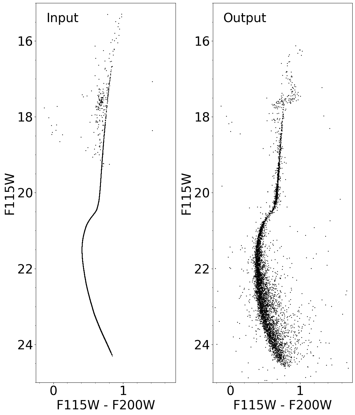
Calibrated Color-Magnitude Diagram#

plt.figure(figsize=(12, 14))
plt.clf()

font2 = {'size': '30'}

ax1 = plt.subplot(1, 2, 1)

mag1_in = np.array(cat_sel['f115w_in'])
mag2_in = np.array(cat_sel['f200w_in'])
diff_in = mag1_in - mag2_in

xlim0 = -0.25
xlim1 = 1.75
ylim0 = 25
ylim1 = 15 
ax1.set_xlim(xlim0, xlim1)
ax1.set_ylim(ylim0, ylim1)

ax1.xaxis.set_major_locator(ticker.AutoLocator())
ax1.xaxis.set_minor_locator(ticker.AutoMinorLocator())
ax1.yaxis.set_major_locator(ticker.AutoLocator())
ax1.yaxis.set_minor_locator(ticker.AutoMinorLocator())

ax1.scatter(mag1_in - mag2_in, mag1_in, s=1, color='k')

ax1.set_xlabel(filt1 + ' - ' + filt2, fontdict=font2)
ax1.set_ylabel(filt1, fontdict=font2)
ax1.text(xlim0 + 0.15, 15.5, "Input", fontdict=font2)

ax2 = plt.subplot(1, 2, 2)

ax2.set_xlim(xlim0, xlim1)
ax2.set_ylim(ylim0, ylim1)

ax2.xaxis.set_major_locator(ticker.AutoLocator())
ax2.xaxis.set_minor_locator(ticker.AutoMinorLocator())
ax2.yaxis.set_major_locator(ticker.AutoLocator())
ax2.yaxis.set_minor_locator(ticker.AutoMinorLocator())

f115w = matched_sources[filt1 + '_inst'] + zp_f115w 
f200w = matched_sources[filt2 + '_inst'] + zp_f200w

maglim = np.arange(18, 25, 1)
mags = []
errs_mag = []
errs_col = []

for i in np.arange(0, len(maglim) - 1, 1):
    mag = (maglim[i] + maglim[i + 1]) / 2
    err_mag1 = matched_sources['e' + filt1 + '_inst'][(f115w > maglim[i]) & (f115w < maglim[i + 1])]
    err_mag2 = matched_sources['e' + filt2 + '_inst'][(f115w > maglim[i]) & (f115w < maglim[i + 1])]
    err_mag = np.mean(err_mag1[i])
    err_temp = np.sqrt(err_mag1**2 + err_mag2**2)
    err_col = np.mean(err_temp[i])

    errs_mag.append(err_mag)                  
    errs_col.append(err_col)
    mags.append(mag)

col = [0] * (len(maglim) - 1)

# ax2.errorbar(col, mags, yerr=errs_mag, xerr=errs_col, fmt='o', color = 'k')
    
ax2.scatter(f115w - f200w, f115w, s=1, color='k')
ax2.text(xlim0 + 0.15, 15.5, "Output", fontdict=font2)

ax2.set_xlabel(filt1 + ' - ' + filt2, fontdict=font2)
ax2.set_ylabel(filt1, fontdict=font2)

plt.tight_layout()

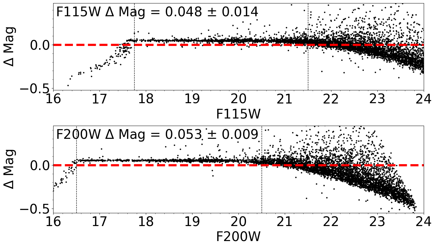
../../_images/5b017c399e8395d09f2e4f40e9ecfa11af5db5efa2db39c75773805a9ac4e6d5.png

Comparison between input and output photometry#

plt.figure(figsize=(14, 8))
plt.clf()

ax1 = plt.subplot(2, 1, 1)

ax1.set_xlabel(filt1, fontdict=font2)
ax1.set_ylabel('$\Delta$ Mag', fontdict=font2)

radec_input = SkyCoord(cat_sel['ra_in'], cat_sel['dec_in'], unit='deg')

idx_f115w_cfr, d2d_f115w_cfr, _ = match_coordinates_sky(radec_input, matched_sources['radec'])

sep_f115w_cfr = d2d_f115w_cfr < max_sep

f115w_inp_cfr = np.array(cat_sel['f115w_in'][sep_f115w_cfr])
f115w_ap_cfr = np.array(f115w[idx_f115w_cfr[sep_f115w_cfr]])

diff_f115w_cfr = f115w_inp_cfr - f115w_ap_cfr
diff_f115w_cfr_sel = (f115w_inp_cfr - f115w_ap_cfr)[(f115w_ap_cfr > 17.75) & (f115w_ap_cfr < 21.5)]

_, med_diff_f115w_cfr, sig_diff_f115w_cfr = sigma_clipped_stats(diff_f115w_cfr_sel)

xlim0 = 16
xlim1 = 24
ylim0 = np.mean(diff_f115w_cfr) - 0.5
ylim1 = np.mean(diff_f115w_cfr) + 0.5

ax1.set_xlim(xlim0, xlim1)
ax1.set_ylim(ylim0, ylim1)

ax1.xaxis.set_major_locator(ticker.AutoLocator())
ax1.xaxis.set_minor_locator(ticker.AutoMinorLocator())
ax1.yaxis.set_major_locator(ticker.AutoLocator())
ax1.yaxis.set_minor_locator(ticker.AutoMinorLocator())

ax1.scatter(f115w_ap_cfr, diff_f115w_cfr, s=5, color='k')
ax1.plot([xlim0, xlim1], [0, 0], color='r', lw=5, ls='--')
ax1.plot([17.75, 17.75], [ylim0, ylim1], color='k', lw=1, ls='--')
ax1.plot([21.5, 21.5], [ylim0, ylim1], color='k', lw=1, ls='--')

ax1.text(xlim0 + 0.05, ylim1 - 0.15, filt1 + ' $\Delta$ Mag = %5.3f $\pm$ %5.3f'
         % (med_diff_f115w_cfr, sig_diff_f115w_cfr), color='k', fontdict=font2)

ax2 = plt.subplot(2, 1, 2)

ax2.set_xlabel(filt2, fontdict=font2)
ax2.set_ylabel('$\Delta$ Mag', fontdict=font2)

idx_f200w_cfr, d2d_f200w_cfr, _ = match_coordinates_sky(radec_input, matched_sources['radec'])

sep_f200w_cfr = d2d_f200w_cfr < max_sep

f200w_inp_cfr = np.array(cat_sel['f200w_in'][sep_f200w_cfr])
f200w_ap_cfr = np.array(f200w[idx_f200w_cfr[sep_f200w_cfr]])

diff_f200w_cfr = f200w_inp_cfr - f200w_ap_cfr
diff_f200w_cfr_sel = (f200w_inp_cfr - f200w_ap_cfr)[(f200w_ap_cfr > 16.5) & (f200w_ap_cfr < 20.5)]

_, med_diff_f200w_cfr, sig_diff_f200w_cfr = sigma_clipped_stats(diff_f200w_cfr_sel)

xlim0 = 16
xlim1 = 24
ylim0 = np.mean(diff_f200w_cfr) - 0.5
ylim1 = np.mean(diff_f200w_cfr) + 0.5

ax2.set_xlim(xlim0, xlim1)
ax2.set_ylim(ylim0, ylim1)

ax2.xaxis.set_major_locator(ticker.AutoLocator())
ax2.xaxis.set_minor_locator(ticker.AutoMinorLocator())
ax2.yaxis.set_major_locator(ticker.AutoLocator())
ax2.yaxis.set_minor_locator(ticker.AutoMinorLocator())

ax2.scatter(f200w_ap_cfr, diff_f200w_cfr, s=5, color='k')
ax2.plot([xlim0, xlim1], [0, 0], color='r', lw=5, ls='--')
ax2.plot([16.5, 16.5], [ylim0, ylim1], color='k', lw=1, ls='--')
ax2.plot([20.5, 20.5], [ylim0, ylim1], color='k', lw=1, ls='--')

ax2.text(xlim0 + 0.05, ylim1 - 0.15, filt2 + ' $\Delta$ Mag = %5.3f $\pm$ %5.3f'
         % (med_diff_f200w_cfr, sig_diff_f200w_cfr), color='k', fontdict=font2)

plt.tight_layout()

../../_images/ef4a61f9f604810cd93d60cabd5471e17b3ad08dd19cd9fc761a96fd8a13d032.png

About this Notebook#

Author: Matteo Correnti, JWST/NIRCam STScI Scientist II
Updated on: 2021-01-15

Top of Page