Exploring High-Redshift Quasars with eBOSS and JWST

---

Learning Goals

By the end of this tutorial, you will:

• Understand how to search the MAST Archive and download SDSS eBOSS data using astroquery.mast

• Learn how to identify emisison lines in quasar spectra at different redshifts

• Download and plot quasar spectra from both eBOSS and JWST

Table of Contents

• Introduction

• Imports

• Accessing eBOSS data at MAST

  • Querying all eBOSS data

  • Searching for a specific target

• Plotting an eBOSS Spectrum

  • Identifying Emission Lines in a QSO Spectrum

  • Exploring QSO spectra at different redshift

• Searching for High-Redshift JWST spectra

  • Combining eBOSS and JWST Data

• Additional Resources

  • How to Cite

  • About This Notebook

Introduction

The Extended Baryonic Oscillaton Spectroscopic Survey (eBOSS) survey provides optical-wavelength 1-D spectra for almost 4,000,000 targets in the northern hemisphere, including stars, galaxies, and quasars. eBOSS collected data between 2008 - 2020 as part of the Sloan Digital Sky Survey (SDSS-IV) project. eBOSS data is now available at the Mikulski Archive for Space Telescopes (MAST) through the SDSS Legacy Archive at MAST.

In this notebook tutorial, we will demonstrate how to access eBOSS data at MAST using Python. One eBOSS target, a quasar named “eBOSS 5733-56575-0260”, will be used to demonstrate the basics of how to download and plot eBOSS data. We will then combine this eBOSS spectrum with infrared spectra from JWST, also accessible from MAST, to study quasars at different redshifts.

Imports

The main packages we’re using for this notebook and their use-cases are:

• astroquery.mast.Observations for searching the MAST archive

• astropy.io fits for accessing FITS files

• matplotlib for plotting and displaying data

• numpy to handle array functions and basic math

%matplotlib inline

from astroquery.mast import Observations
import astropy.io.fits as fits

import matplotlib.pyplot as plt
from matplotlib.colors import LogNorm
import matplotlib.patheffects as path_effects
from matplotlib.patches import ConnectionPatch

import numpy as np

This cell updates some of the settings in matplotlib to use larger font sizes in the figures:

#Update Plotting Parameters
params = {'axes.labelsize': 12, 'xtick.labelsize': 12, 'ytick.labelsize': 12, 
          'text.usetex': False, 'lines.linewidth': 1,
          'axes.titlesize': 18, 'font.family': 'serif', 'font.size': 12}
plt.rcParams.update(params)

---

Accessing eBOSS data at MAST

The SDSS Legacy Archive at MAST hosts all of the science-ready data products from the SDSS-IV eBOSS Survey, which includes optical-wavelength spectra for almost 4,000,000 targets in northern hemisphere, including stars, galaxies and quasi-stellar objects (QSOs). This notebook will demonstrate how to search and download eBOSS data using MAST!

Querying all eBOSS data

Searching for eBOSS data is straightforward with astroquery.mast. In this example, we use Observations.query_criteria and search for provenance_name = 'eBOSS' (this is not case sensitive; eboss or EBOSS will also work). This will return a table describing all of the eBOSS data hosted by the MAST archive.

Other useful search parameters for eBOSS data might include:

• obs_collection = 'SDSS': searches for all SDSS data

• Use target_name to search for stars using their eBOSS identifiers, usually in the form eBOSS {PLATE}-{MJD}-{FIBER}, for example eBOSS 12547-58928-1.

• The target_classification provides basic information on what this target was indentified as (“QSO”, “STAR”, or “GALAXY”) in the eBOSS pipeline.

• obs_id can help search for specific targets or fields. Note that wild cards (*) are allowed in the search fields, for example, obs_id='sdss_eboss_12547-*' will search for everything observed on the plate numbered 12547

Here we also use the pagesize=10 and page=1 parameters to limit the number of results - otherwise, there are nearly 4,000,000 eBOSS observations in MAST! This query might take a few minutes to run.

# Search for eBOSS data
eboss_obs_list = Observations.query_criteria(provenance_name='eBOSS', page=1, pagesize=10)

# Display First Ten Entries in Table
eboss_obs_list

Table masked=True length=10

intentType	obs_collection	provenance_name	instrument_name	project	filters	wavelength_region	target_name	target_classification	obs_id	s_ra	s_dec	dataproduct_type	proposal_pi	calib_level	t_min	t_max	t_exptime	em_min	em_max	obs_title	t_obs_release	proposal_id	proposal_type	sequence_number	s_region	jpegURL	dataURL	dataRights	mtFlag	srcDen	obsid	objID
str7	str4	str5	str4	str4	str4	str7	str20	str6	str26	float64	float64	str8	str18	int64	float64	float64	float64	float64	float64	str56	float64	str3	str1	int64	str56	str62	str62	str6	bool	float64	str9	str9
science	SDSS	eBOSS	BOSS	SDSS	None	OPTICAL	eBOSS 4495-55566-505	QSO	sdss_eboss_4495-55566-0505	116.79055	16.352739	spectrum	SDSS Collaboration	3	55565.27777777778	55566.315253125	4504.22	360.0	1040.0	Extended Baryon Oscillation Spectroscopic Survey (eBOSS)	59554.0	N/A	--	--	CIRCLE 116.79055 16.352739 0.0002777777777777778	mast:SDSS/eboss/4495/55566/0505/spec-image-4495-55566-0505.png	mast:SDSS/eboss/4495/55566/0505/full/spec-4495-55566-0505.fits	PUBLIC	False	nan	244400518	725345081
science	SDSS	eBOSS	BOSS	SDSS	None	OPTICAL	eBOSS 4987-55746-369	GALAXY	sdss_eboss_4987-55746-0369	253.24208	33.325365	spectrum	SDSS Collaboration	3	55744.314351851855	55746.340993287035	6305.76	360.0	1040.0	Extended Baryon Oscillation Spectroscopic Survey (eBOSS)	59554.0	N/A	--	--	CIRCLE 253.24208 33.325365 0.0002777777777777778	mast:SDSS/eboss/4987/55746/0369/spec-image-4987-55746-0369.png	mast:SDSS/eboss/4987/55746/0369/full/spec-4987-55746-0369.fits	PUBLIC	False	nan	244400519	725345084
science	SDSS	eBOSS	BOSS	SDSS	None	OPTICAL	eBOSS 6187-56244-250	GALAXY	sdss_eboss_6187-56244-0250	8.01335499999999	18.783668	spectrum	SDSS Collaboration	3	56244.1996875	56244.2556	4504.22	360.0	1040.0	Extended Baryon Oscillation Spectroscopic Survey (eBOSS)	59554.0	N/A	--	--	CIRCLE 8.01335499999999 18.783668 0.0002777777777777778	mast:SDSS/eboss/6187/56244/0250/spec-image-6187-56244-0250.png	mast:SDSS/eboss/6187/56244/0250/full/spec-6187-56244-0250.fits	PUBLIC	False	nan	244400520	725345088
science	SDSS	eBOSS	BOSS	SDSS	None	OPTICAL	eBOSS 4495-55566-538	GALAXY	sdss_eboss_4495-55566-0538	117.09453	16.059239	spectrum	SDSS Collaboration	3	55565.27777777778	55566.315253125	4504.22	360.0	1040.0	Extended Baryon Oscillation Spectroscopic Survey (eBOSS)	59554.0	N/A	--	--	CIRCLE 117.09453 16.059239 0.0002777777777777778	mast:SDSS/eboss/4495/55566/0538/spec-image-4495-55566-0538.png	mast:SDSS/eboss/4495/55566/0538/full/spec-4495-55566-0538.fits	PUBLIC	False	nan	244400521	725345091
science	SDSS	eBOSS	BOSS	SDSS	None	OPTICAL	eBOSS 4987-55746-710	QSO	sdss_eboss_4987-55746-0710	253.8215	35.637936	spectrum	SDSS Collaboration	3	55744.314351851855	55746.34099351852	6305.76	360.0	1040.0	Extended Baryon Oscillation Spectroscopic Survey (eBOSS)	59554.0	N/A	--	--	CIRCLE 253.8215 35.637936 0.0002777777777777778	mast:SDSS/eboss/4987/55746/0710/spec-image-4987-55746-0710.png	mast:SDSS/eboss/4987/55746/0710/full/spec-4987-55746-0710.fits	PUBLIC	False	nan	244400522	725345092
science	SDSS	eBOSS	BOSS	SDSS	None	OPTICAL	eBOSS 6187-56244-390	QSO	sdss_eboss_6187-56244-0390	7.325178300000005	19.662345	spectrum	SDSS Collaboration	3	56244.1996875	56244.2556	4504.22	360.0	1040.0	Extended Baryon Oscillation Spectroscopic Survey (eBOSS)	59554.0	N/A	--	--	CIRCLE 7.325178300000005 19.662345 0.0002777777777777778	mast:SDSS/eboss/6187/56244/0390/spec-image-6187-56244-0390.png	mast:SDSS/eboss/6187/56244/0390/full/spec-6187-56244-0390.fits	PUBLIC	False	nan	244400523	725345094
science	SDSS	eBOSS	BOSS	SDSS	None	OPTICAL	eBOSS 4495-55566-296	QSO	sdss_eboss_4495-55566-0296	118.1186	15.415375	spectrum	SDSS Collaboration	3	55565.27777777778	55566.31525277778	4504.22	360.0	1040.0	Extended Baryon Oscillation Spectroscopic Survey (eBOSS)	59554.0	N/A	--	--	CIRCLE 118.1186 15.415375 0.0002777777777777778	mast:SDSS/eboss/4495/55566/0296/spec-image-4495-55566-0296.png	mast:SDSS/eboss/4495/55566/0296/full/spec-4495-55566-0296.fits	PUBLIC	False	nan	244400524	725345097
science	SDSS	eBOSS	BOSS	SDSS	None	OPTICAL	eBOSS 4987-55746-1	GALAXY	sdss_eboss_4987-55746-0001	255.54894	33.805452	spectrum	SDSS Collaboration	3	55744.314351851855	55746.340993287035	6305.76	360.0	1040.0	Extended Baryon Oscillation Spectroscopic Survey (eBOSS)	59554.0	N/A	--	--	CIRCLE 255.54894 33.805452 0.0002777777777777778	mast:SDSS/eboss/4987/55746/0001/spec-image-4987-55746-0001.png	mast:SDSS/eboss/4987/55746/0001/full/spec-4987-55746-0001.fits	PUBLIC	False	nan	244400525	725345098
science	SDSS	eBOSS	BOSS	SDSS	None	OPTICAL	eBOSS 6187-56244-151	GALAXY	sdss_eboss_6187-56244-0151	8.459340499999996	19.569845	spectrum	SDSS Collaboration	3	56244.1996875	56244.2556	4504.22	360.0	1040.0	Extended Baryon Oscillation Spectroscopic Survey (eBOSS)	59554.0	N/A	--	--	CIRCLE 8.459340499999996 19.569845 0.0002777777777777778	mast:SDSS/eboss/6187/56244/0151/spec-image-6187-56244-0151.png	mast:SDSS/eboss/6187/56244/0151/full/spec-6187-56244-0151.fits	PUBLIC	False	nan	244400526	725345101
science	SDSS	eBOSS	BOSS	SDSS	None	OPTICAL	eBOSS 4495-55566-547	GALAXY	sdss_eboss_4495-55566-0547	117.12188	17.009968	spectrum	SDSS Collaboration	3	55565.27777777778	55566.315253125	4504.22	360.0	1040.0	Extended Baryon Oscillation Spectroscopic Survey (eBOSS)	59554.0	N/A	--	--	CIRCLE 117.12188 17.009968 0.0002777777777777778	mast:SDSS/eboss/4495/55566/0547/spec-image-4495-55566-0547.png	mast:SDSS/eboss/4495/55566/0547/full/spec-4495-55566-0547.fits	PUBLIC	False	nan	244400527	725345103

Searching for a specific target

Let’s narrow down the search to look at one particular target: a high-redshift quasar (QSO) named “eBOSS 5733-56575-0260”. Quasars are a type of active galactic nuclei: supermassive black holes which are actively accreting material, producing bright spectra characterized by strong emission lines. Because quasars are so bright, they can be observed at large distances, which make them useful for studying the large-scale structure of the Universe and the most distant galaxies.

We can search for this quasar in particular using the obs_id keyword:

# Search for all QSOs
eboss_obs_list = Observations.query_criteria(provenance_name='eBOSS', # Query eBOSS data
                                             target_classification='QSO', # Search for quasars
                                             obs_id='sdss_eboss_5733-56575-0260' # Search for a specific target using obs_id
                                             )

# Display results
eboss_obs_list

Table masked=True length=1

intentType	obs_collection	provenance_name	instrument_name	project	filters	wavelength_region	target_name	target_classification	obs_id	s_ra	s_dec	dataproduct_type	proposal_pi	calib_level	t_min	t_max	t_exptime	em_min	em_max	obs_title	t_obs_release	proposal_id	proposal_type	sequence_number	s_region	jpegURL	dataURL	dataRights	mtFlag	srcDen	obsid	objID
str7	str4	str5	str4	str4	str4	str7	str20	str3	str26	float64	float64	str8	str18	int64	float64	float64	float64	float64	float64	str56	float64	str3	str1	int64	str48	str62	str62	str6	bool	float64	str9	str9
science	SDSS	eBOSS	BOSS	SDSS	None	OPTICAL	eBOSS 5733-56575-260	QSO	sdss_eboss_5733-56575-0260	138.79167	47.949732	spectrum	SDSS Collaboration	3	56572.46884259259	56575.492721296294	5400.68	360.0	1040.0	Extended Baryon Oscillation Spectroscopic Survey (eBOSS)	59554.0	N/A	--	--	CIRCLE 138.79167 47.949732 0.0002777777777777778	mast:SDSS/eboss/5733/56575/0260/spec-image-5733-56575-0260.png	mast:SDSS/eboss/5733/56575/0260/full/spec-5733-56575-0260.fits	PUBLIC	False	nan	244396372	725334231

From this results table, we can see some basic metadata related to this observation:

• It’s coordinates are in the s_ra and s_dec columns

• This spectrum was observed using the BOSS instrument (instrument_name)

• This target is classified as a QSO (target_classification)

• From the t_min column, we can see that this star was first observed on the date of MJD 56572 (Correpsonding to 2013-10-07) and last observed on MJD 56575 (2013-10-10)

• eBOSS provides optical-wavelength (wavelength_region) spectra (dataproduct_type) with wavelength range of 360.0 - 1040.0 nanometers (em_min, em_max)

Downloading eBOSS data products

List all of the data products availble for this observation using Observations.get_product_list().

There are 3 total files available for this quasar, which includes the “full spectrum” file, the “lite spectrum” file, and a preview image. Only the full spectrum is tagged as “Minimum Recommended Products”. More information on the eBOSS data products available at MAST can be found on the eBOSS Data Products in the Archive Manual, and more information on all of these products can be seen in the search results table:

# List all products available for this observation
products = Observations.get_product_list(eboss_obs_list)

# Show table
products

Table masked=True length=5

obsID	obs_collection	dataproduct_type	obs_id	description	type	dataURI	productType	productGroupDescription	productSubGroupDescription	productDocumentationURL	project	prvversion	proposal_id	productFilename	size	parent_obsid	dataRights	calib_level	filters
str9	str4	str12	str29	str235	str1	str67	str7	str28	str14	str48	str5	str7	str3	str30	int64	str9	str6	int64	str4
244396372	SDSS	spectrum	sdss_eboss_5733-56575-0260	Preview-Full	S	mast:SDSS/eboss/5733/56575/0260/spec-image-5733-56575-0260.png	PREVIEW	--	--	--	eBOSS	DR17	N/A	spec-image-5733-56575-0260.png	39826	244396372	PUBLIC	3	None
244396372	SDSS	spectrum	sdss_eboss_5733-56575-0260	SDSS eBOSS lite spectrum file containing the combined spectrum and associated metadata but not the individual exposures.	S	mast:SDSS/eboss/5733/56575/0260/lite/spec-lite-5733-56575-0260.fits	SCIENCE	--	SPECTRA	https://archive.stsci.edu/missions-and-data/sdss	eBOSS	DR17	N/A	spec-lite-5733-56575-0260.fits	218880	244396372	PUBLIC	3	None
244396372	SDSS	spectrum	sdss_eboss_5733-56575-0260	SDSS eBOSS full spectrum file containing the combined spectrum, associated metadata, and the individual exposures.	S	mast:SDSS/eboss/5733/56575/0260/full/spec-5733-56575-0260.fits	SCIENCE	Minimum Recommended Products	SPECTRA	https://archive.stsci.edu/missions-and-data/sdss	eBOSS	DR17	N/A	spec-5733-56575-0260.fits	1514880	244396372	PUBLIC	3	None
252284571	SDSS	measurements	sdss_eboss_spzall_5733-56575	SDSS eBOSS summary catalog, for each plate-MJD, containing the best fits for spectral redshift and classification measurements, rank-ordered by chi-squared. If the best fit looks bad from the spAll file, check the second best fit here.	D	mast:SDSS/eboss/5733/56575/spZall-5733-56575.fits	SCIENCE	--	eBOSS Catalogs	https://archive.stsci.edu/missions-and-data/sdss	eBOSS	v5_13_2	N/A	spZall-5733-56575.fits	128540160	244396372	PUBLIC	3	--
252284572	SDSS	measurements	sdss_eboss_spplate_5733-56575	SDSS eBOSS summary catalog, for each plate-MJD, containing the combined spectra and targeting information for all observations on a single plate.	D	mast:SDSS/eboss/5733/56575/spPlate-5733-56575.fits	SCIENCE	--	eBOSS Catalogs	https://archive.stsci.edu/missions-and-data/sdss	eBOSS	v5_13_2	N/A	spPlate-5733-56575.fits	112003200	244396372	PUBLIC	3	--

Now we will download the spectrum for this quasar using Observations.download_products(). The download will print a status message when completed.

manifest = Observations.download_products(products, mrp_only=True)

Downloading URL https://mast.stsci.edu/api/v0.1/Download/file?uri=mast:SDSS/eboss/5733/56575/0260/full/spec-5733-56575-0260.fits to ./mastDownload/SDSS/sdss_eboss_5733-56575-0260/spec-5733-56575-0260.fits ...

 [Done]

---

Plotting an eBOSS Spectrum

Now let’s take a look at the file and plot the spectrum.

Based on the descriptions in the eBOSS Spectrum Data Model, this file has several extensions, corresponding to the metadata, the co-added spectrum, some catalog information, and the individual visit exposures:

• HDU0: “PRIMARY”: The Primary Header and file metadata

• HDU1: “COADD”: The array containing the coadded observed spectrum

• HDU2: “SPALL”: Summary metadata about this target, including targeting information, spectroscopic classifications, and redshifts for this target

• HDU3: “SPZLINE”: Line fitting metadata about the target: contains measurements of emission lines and redshift output from the SDSS Spectro-1D analysis pipeline.

• HDU4+ : The rest of the file extensions contain the individual frames from each exposure that went into the coadded spectrum: “B” for the blue chip and “R” for the red chip of each exposure.

# Open file
eboss_spectrum = fits.open(manifest['Local Path'][0])

# Display file information
eboss_spectrum.info()

Filename: ./mastDownload/SDSS/sdss_eboss_5733-56575-0260/spec-5733-56575-0260.fits
No.    Name      Ver    Type      Cards   Dimensions   Format
  0  PRIMARY       1 PrimaryHDU     129   ()      
  1  COADD         1 BinTableHDU     26   4628R x 8C   [E, E, E, J, J, E, E, E]   
  2  SPALL         1 BinTableHDU    488   1R x 236C   [27A, 14A, 4A, E, E, J, J, E, J, E, E, E, K, K, K, K, K, K, K, K, K, B, B, J, I, 5E, 5E, J, J, J, J, 7A, 7A, 16A, D, D, 6A, 21A, E, E, E, J, E, 24A, 10J, J, 10E, E, E, E, E, E, E, J, E, E, E, J, 5E, E, E, 10E, 10E, 10E, 5E, 5E, 5E, 5E, 5E, J, J, E, E, E, E, E, E, 16A, 9A, 12A, E, E, E, E, E, E, E, E, J, E, E, J, J, 6A, 21A, E, 35E, K, 19A, 19A, 19A, B, B, B, I, 3A, B, I, I, I, I, J, E, J, J, E, E, E, E, E, E, E, E, 5E, 5E, 5E, 5E, 5E, 5E, 5E, 5E, 5E, 5E, 5E, 5E, 5E, 5E, 5E, 5E, 5E, 5E, 5E, 5E, 5E, 5E, 5E, 5E, 5E, 5E, 5E, 5E, 5E, 5E, 5E, 5E, 5E, 5E, 5E, 5J, 5J, 5J, 5E, 5J, 75E, 75E, 5E, 5E, 5E, 5J, 5E, D, D, D, D, D, D, D, D, D, 5E, 5E, 5E, 5E, 5E, 5E, 5E, 5E, 5E, 5E, 5E, 5E, 5E, 5E, 5E, 5E, 5E, 5E, 5E, 5E, 5E, 5E, 5E, 5E, 5E, 5E, 5E, 5E, 5E, 5E, 5E, 5E, 5E, 5E, 5E, 5E, 5E, 5E, 5E, 5E, 5E, 5E, 40E, 40E, 5J, 5J, 5E, 5E, 5D, J, J, J, J, J, J, J, E]   
  3  SPZLINE       1 BinTableHDU     48   32R x 19C   [J, J, J, 13A, D, E, E, E, E, E, E, E, E, E, E, J, J, E, E]   
  4  B1-00167523-00167522-00167521    1 BinTableHDU    181   2516R x 8C   [E, E, E, J, E, E, E, E]   
  5  B1-00167524-00167522-00167521    1 BinTableHDU    181   2516R x 8C   [E, E, E, J, E, E, E, E]   
  6  B1-00167695-00167694-00167693    1 BinTableHDU    181   2516R x 8C   [E, E, E, J, E, E, E, E]   
  7  B1-00167696-00167694-00167693    1 BinTableHDU    181   2516R x 8C   [E, E, E, J, E, E, E, E]   
  8  B1-00167697-00167694-00167693    1 BinTableHDU    181   2516R x 8C   [E, E, E, J, E, E, E, E]   
  9  B1-00167762-00167761-00167760    1 BinTableHDU    181   2515R x 8C   [E, E, E, J, E, E, E, E]   
 10  R1-00167523-00167522-00167521    1 BinTableHDU    181   3129R x 8C   [E, E, E, J, E, E, E, E]   
 11  R1-00167524-00167522-00167521    1 BinTableHDU    181   3130R x 8C   [E, E, E, J, E, E, E, E]   
 12  R1-00167695-00167694-00167693    1 BinTableHDU    181   3126R x 8C   [E, E, E, J, E, E, E, E]   
 13  R1-00167696-00167694-00167693    1 BinTableHDU    181   3128R x 8C   [E, E, E, J, E, E, E, E]   
 14  R1-00167697-00167694-00167693    1 BinTableHDU    181   3128R x 8C   [E, E, E, J, E, E, E, E]   
 15  R1-00167762-00167761-00167760    1 BinTableHDU    181   3123R x 8C   [E, E, E, J, E, E, E, E]   

We can plot the spectrum using this information! The wavelength and flux data are all found in the first extension (HDU1: “COADD”).

fig, ax = plt.subplots(figsize=(15, 5))

# Define wavelengths
# eBOSS wavelengths are in log space - convert to linear
wls = 10**eboss_spectrum[1].data['loglam']

# Get the observed and model flux from extension 1
observed_flux = eboss_spectrum[1].data['flux']
model_flux = eboss_spectrum[1].data['model']

# Plot the observed spectrum
plt.plot(wls, observed_flux, c='gray', label='Observed Spectrum')
# Plot the model spectrum
plt.plot(wls, model_flux, c='k', label='Model Spectrum')

# Set title and labels
plt.title(f"{eboss_obs_list['target_name'][0]}")
redshift = eboss_spectrum[2].data['Z'][0] # redshift from SPALL table
plt.text(0.02, 0.95, f"z = {str(round(redshift, 2))}", 
         fontsize=24, ha='left', va='top', transform=ax.transAxes)
plt.xlabel(r'Wavelength [$\AA$]')
plt.grid() # Add grid lines
plt.legend(loc='upper right') # Add plot legend
plt.show() # Display plot

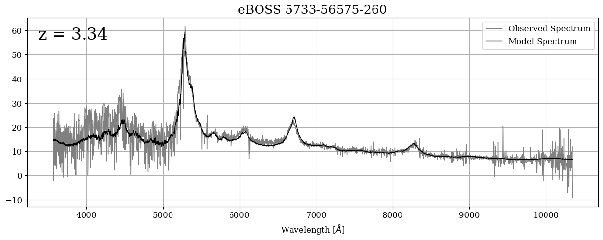
The eBOSS spectrum for this QSO looks great! The large spikes around 5200, 6700, and 8200 angstroms are strong emission lines from the accretion disk around the supermassive black hole in the center of this QSO. We can identify which emission lines they are by using the quasar’s redshift, which we will do next.

Identifying Emission Lines in a QSO Spectrum

Let’s spruce up this plot by adding labels on the emission lines, and plotting a second panel which shows the brightness (flux) as color instead of a line.

To help with identifying the emision lines, let’s write a helper function to define and plot the emission lines we want to label, called plot_emission_lines(). Becasue this quasar is so far away, the emission lines will be redshifted, meaning the observed wavelength might be far away from the rest wavelength!

The equation for calculating the observed wavelength of an emission line at redshift \(z\) is:

\begin{equation} 1+z = \frac{\lambda_{observed}}{\lambda_{emitted}} \end{equation}

where \(\lambda_{emitted}\) is the rest-frame wavelength of the emission line, and \(z\) is the redshift. We will use this equation to convert between rest wavelength and observed wavelength in our helper function.

# Create a dictionary of emission lines we want to label
# These line definitions are from the eBOSS pipeline: https://data.sdss.org/datamodel/files/SPECTRO_REDUX/RUN2D/PLATE4/spZline.html
emission_line_list = [
    {
        'emline': r'Lyman-$\alpha$',
        'rest_wavelength': 1215.67,
        'label_color': 'purple',
        'label_index': 16,
        'label_angle': 35,
    },
    {
        'emline': 'C IV',
        'rest_wavelength': 1549.487,
        'label_color': 'mediumblue',
        'label_index': 14,
        'label_angle': 35,
    },
    {
        'emline': '[C III]',
        'rest_wavelength': 1908.734,
        'label_color': 'deepskyblue',
        'label_index': 12,
        'label_angle': 25,
    },
    {
        'emline': 'Mg II',
        'rest_wavelength': 2800.31518862,
        'label_color': 'green',
        'label_index': 8,
        'label_angle': 20,
    },
    {
        'emline': '[O III]',
        'rest_wavelength': 5008.23966962,
        'label_color': 'darkorange',
        'label_index': 2,
        'label_angle': 10,
    },
    {
        'emline': r'H-$\alpha$',
        'rest_wavelength': 6564.61397371,
        'label_color': 'red',
        'label_index': 1,
        'label_angle': 10,
        }
    ]


def plot_emission_lines(ax: plt.axes, redshift: float) -> None:
    """
    Helper function to plot emission line references on a figure.

    Parameters:
    ============
    ax: 
        The axes object to draw on
    redshift:
        the redshift (z) of the QSO which determines how much to shift the lines
        from the rest wavelength to the observed wavelength.
    """    
    # Plot and Label the emission lines
    for emline in emission_line_list:
        # Calculate observed wavelength from quasar redshift
        observed_wavelength = (1+redshift)*emline['rest_wavelength']
        # If the observed wavelength is within the limits of the plot, plot it!
        if (observed_wavelength >= np.min(wls)) & (observed_wavelength <= np.max(wls)):
            ax.axvline(observed_wavelength, c=emline['label_color'], linestyle='--', lw=2)
            ax.axvline(observed_wavelength, c=emline['label_color'], linestyle='--', lw=2)
            ax.text(observed_wavelength, 0.98, emline['emline'],
                    color=emline['label_color'], rotation=90, ha='right', va='top', fontsize=16,
                    transform=ax.get_xaxis_transform())

In the next cell, we plot the spectrum again adding these new features.

# Set up spectrum plot
fig = plt.figure(figsize=(15, 5))
ax1 = plt.subplot2grid((5, 1), (0, 0), colspan=1, rowspan=4)
ax2 = plt.subplot2grid((5, 1), (4, 0), colspan=1, rowspan=1)

# Open spectrum file
eboss_spectrum = fits.open(manifest['Local Path'][0])
# Define QSO name
eboss_id = f"{eboss_spectrum[0].header['PLATEID']}-{eboss_spectrum[0].header['MJD']}-{eboss_spectrum[0].header['FIBERID']}"
# Retrieve redshift from SPALL table
redshift = eboss_spectrum[2].data['Z'][0] 

# Define wavelengths
wls = 10**eboss_spectrum[1].data['loglam']
# Get the observed and model flux from extension 1
observed_flux = eboss_spectrum[1].data['flux']
model_flux = eboss_spectrum[1].data['model']


# Plot the observed spectrum
ax1.plot(wls, observed_flux, c='gray', label='Observed Spectrum')
# Plot the model spectrum
ax1.plot(wls, model_flux, c='k', label='Model Spectrum')
# Normalize the flux for the colobar
normalized_flux = (model_flux/np.max(model_flux))
ax2.pcolormesh(wls, [0, 1], [normalized_flux, normalized_flux],
               norm=LogNorm(), cmap='magma')

# Plot emission lines
plot_emission_lines(ax1, redshift)

# Set title and labels
ax1.set_title(f"eBOSS spectrum - {eboss_id}")
# Add redshift to plot
ax1.text(0.02, 0.95, f"z = {str(round(redshift, 2))}", 
         fontsize=24, ha='left', va='top', transform=ax1.transAxes)
ax2.set_xlabel(r'Wavelength [$\AA$]')
ax2.set_yticks([])
ax1.set_ylabel('Flux')
ax1.grid() # Add grid lines
ax1.legend(loc='upper right') # Add plot legend
# Set axes limits
ax1.set_xlim(np.min(wls), np.max(wls))
ax2.set_xlim(np.min(wls), np.max(wls))
ax1.set_ylim(0, np.max(observed_flux))
plt.subplots_adjust(hspace=0) # remove space between plots

plt.show() # Display Plot

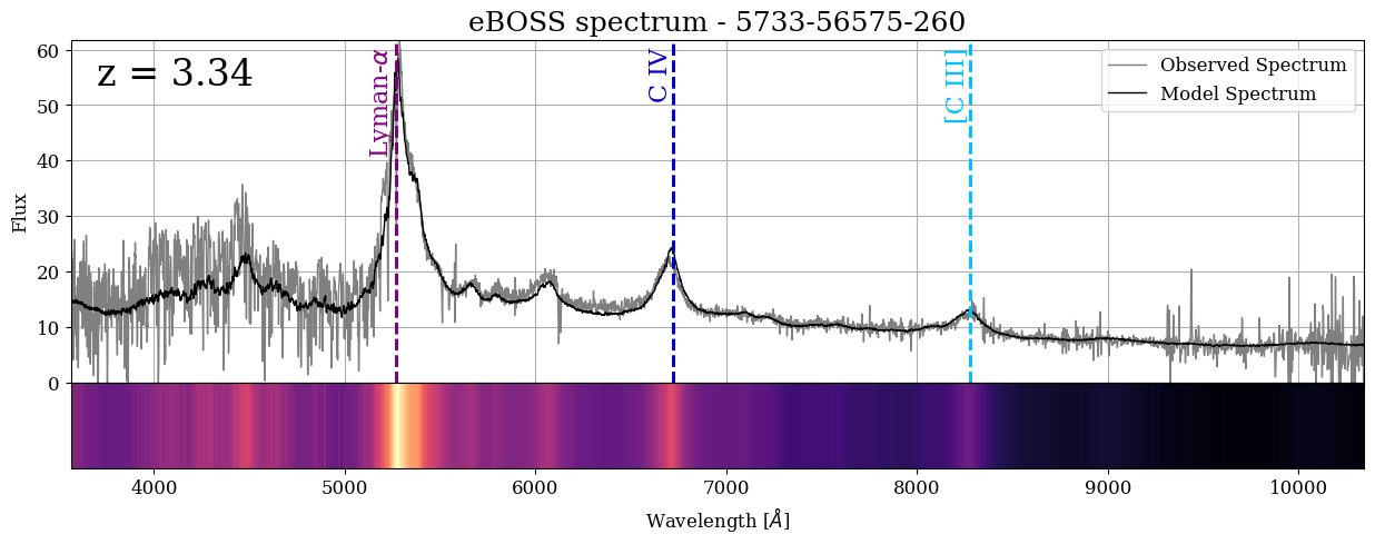
The top panel of our figure shows the spectrum as a line plot, where the bottom panel shows it as a color plot. The higher the flux is in the top panel, the brighter yellow color it is in the bottom panel: two different ways of looking at the same spectrum. With this plot, we can see that the three brightest emission lines in this QSO are Lyman-\(\alpha\), C IV and [C III]!

Exploring QSO spectra at different redshift

Now that we’ve demonstrated how to search, download, and plot a quasar spectrum from eBOSS, let’s repeat this process and look at several QSOs across cosmic time. Our goal is to explore how different characteristics of quasar spectra evolve over time, from the closest to us (low redshift) to farthest away (high redshift).

Here is a list of eBOSS QSOs from a sampling of different redshifts curated for this exercise:

eboss_qso_list = [
    'sdss_eboss_12547-58928-0063', # redshift z = 0.25
    'sdss_eboss_12547-58928-0268', # redshift z = 0.49
    'sdss_eboss_3846-55327-0212', # z = 0.71
    'sdss_eboss_12547-58928-0707', # z = 1.0
    'sdss_eboss_12547-58928-0771', # z = 1.23
    'sdss_eboss_12547-58928-0178', # z = 1.49
    'sdss_eboss_12547-58928-0349', # z =  1.75
    'sdss_eboss_12547-58928-0029', # z = 2.04
    'sdss_eboss_3586-55181-0080', # z = 2.25
    'sdss_eboss_3586-55181-0162', # z = 2.48
    'sdss_eboss_3586-55181-0516', # z = 2.75
    'sdss_eboss_12547-58928-0478', # z = 2.97
    'sdss_eboss_3788-55246-0056', # z = 3.26
    'sdss_eboss_3846-55327-0080', # z =  3.49
    'sdss_eboss_12547-58928-0484', # z = 3.73
    'sdss_eboss_10737-58254-0984', # z = 3.99
    'sdss_eboss_7238-56660-0542', # z = 4.27
    'sdss_eboss_8789-57358-0092', # z = 4.5 
    'sdss_eboss_3588-55184-0548', # z = 4.71
    'sdss_eboss_8528-57896-0104', # z = 5.00
    'sdss_eboss_10256-58193-0330', # z = 5.26
    'sdss_eboss_6782-56602-0526', # z = 5.48
    'sdss_eboss_11315-58402-0842', # z = 5.76
    'sdss_eboss_6667-56412-0676', # z = 6
]

For each of these quasars, we will download the spectra using astroquery.mast and plot them as a color plot like we did before. Only this time, we are going to plot them all on the same figure to see how quasar spectra change over redshift!

def get_eboss_qso_spectrum(eboss_obs_id: str):
    """
    Given an eBOSS observation ID, query MAST and download the spectrum using astroquery.mast

    Parameters:
    =============
    eboss_obs_id: str
        Name of the target / observation ID to search on.

    Returns:
    =============
    dictionary of...    
    """
    # Query MAST for eBOSS observation
    obs_list = Observations.query_criteria(provenance_name='eBOSS', # Query eBOSS data
                                           obs_id=eboss_obs_id) # Search for a specific target
    
    # Retrieve products
    products = Observations.get_product_list(obs_list)
    # Download spectrum file
    manifest = Observations.download_products(products, mrp_only=True)

    eboss_spectrum = fits.open(manifest['Local Path'][0])
    z = eboss_spectrum[2].data['Z'][0] # redshift from SPALL table
    wls = 10**eboss_spectrum[1].data['loglam']
    model_flux = eboss_spectrum[1].data['model']
    normalized_flux = model_flux/np.max(model_flux)
    
    # Define a dictionary with the spectrum and other information we want to save
    qso_spec = {
        "name":  f"eBOSS {eboss_obs_id.split('_')[-1]}",
        "spectrum_filename": manifest['Local Path'],
        "redshift": z,
        "wls": wls,
        "flux": normalized_flux,
        }

    return qso_spec    


all_qsos = [get_eboss_qso_spectrum(obs_id) for obs_id in eboss_qso_list]

Downloading URL https://mast.stsci.edu/api/v0.1/Download/file?uri=mast:SDSS/eboss/12547/58928/0063/full/spec-12547-58928-0063.fits to ./mastDownload/SDSS/sdss_eboss_12547-58928-0063/spec-12547-58928-0063.fits ...

 [Done]

Downloading URL https://mast.stsci.edu/api/v0.1/Download/file?uri=mast:SDSS/eboss/12547/58928/0268/full/spec-12547-58928-0268.fits to ./mastDownload/SDSS/sdss_eboss_12547-58928-0268/spec-12547-58928-0268.fits ...

 [Done]

Downloading URL https://mast.stsci.edu/api/v0.1/Download/file?uri=mast:SDSS/eboss/3846/55327/0212/full/spec-3846-55327-0212.fits to ./mastDownload/SDSS/sdss_eboss_3846-55327-0212/spec-3846-55327-0212.fits ...

 [Done]

Downloading URL https://mast.stsci.edu/api/v0.1/Download/file?uri=mast:SDSS/eboss/12547/58928/0707/full/spec-12547-58928-0707.fits to ./mastDownload/SDSS/sdss_eboss_12547-58928-0707/spec-12547-58928-0707.fits ...

 [Done]

Downloading URL https://mast.stsci.edu/api/v0.1/Download/file?uri=mast:SDSS/eboss/12547/58928/0771/full/spec-12547-58928-0771.fits to ./mastDownload/SDSS/sdss_eboss_12547-58928-0771/spec-12547-58928-0771.fits ...

 [Done]

Downloading URL https://mast.stsci.edu/api/v0.1/Download/file?uri=mast:SDSS/eboss/12547/58928/0178/full/spec-12547-58928-0178.fits to ./mastDownload/SDSS/sdss_eboss_12547-58928-0178/spec-12547-58928-0178.fits ...

 [Done]

Downloading URL https://mast.stsci.edu/api/v0.1/Download/file?uri=mast:SDSS/eboss/12547/58928/0349/full/spec-12547-58928-0349.fits to ./mastDownload/SDSS/sdss_eboss_12547-58928-0349/spec-12547-58928-0349.fits ...

 [Done]

Downloading URL https://mast.stsci.edu/api/v0.1/Download/file?uri=mast:SDSS/eboss/12547/58928/0029/full/spec-12547-58928-0029.fits to ./mastDownload/SDSS/sdss_eboss_12547-58928-0029/spec-12547-58928-0029.fits ...

 [Done]

Downloading URL https://mast.stsci.edu/api/v0.1/Download/file?uri=mast:SDSS/eboss/3586/55181/0080/full/spec-3586-55181-0080.fits to ./mastDownload/SDSS/sdss_eboss_3586-55181-0080/spec-3586-55181-0080.fits ...

 [Done]

Downloading URL https://mast.stsci.edu/api/v0.1/Download/file?uri=mast:SDSS/eboss/3586/55181/0162/full/spec-3586-55181-0162.fits to ./mastDownload/SDSS/sdss_eboss_3586-55181-0162/spec-3586-55181-0162.fits ...

 [Done]

Downloading URL https://mast.stsci.edu/api/v0.1/Download/file?uri=mast:SDSS/eboss/3586/55181/0516/full/spec-3586-55181-0516.fits to ./mastDownload/SDSS/sdss_eboss_3586-55181-0516/spec-3586-55181-0516.fits ...

 [Done]

Downloading URL https://mast.stsci.edu/api/v0.1/Download/file?uri=mast:SDSS/eboss/12547/58928/0478/full/spec-12547-58928-0478.fits to ./mastDownload/SDSS/sdss_eboss_12547-58928-0478/spec-12547-58928-0478.fits ...

 [Done]

Downloading URL https://mast.stsci.edu/api/v0.1/Download/file?uri=mast:SDSS/eboss/3788/55246/0056/full/spec-3788-55246-0056.fits to ./mastDownload/SDSS/sdss_eboss_3788-55246-0056/spec-3788-55246-0056.fits ...

 [Done]

Downloading URL https://mast.stsci.edu/api/v0.1/Download/file?uri=mast:SDSS/eboss/3846/55327/0080/full/spec-3846-55327-0080.fits to ./mastDownload/SDSS/sdss_eboss_3846-55327-0080/spec-3846-55327-0080.fits ...

 [Done]

Downloading URL https://mast.stsci.edu/api/v0.1/Download/file?uri=mast:SDSS/eboss/12547/58928/0484/full/spec-12547-58928-0484.fits to ./mastDownload/SDSS/sdss_eboss_12547-58928-0484/spec-12547-58928-0484.fits ...

 [Done]

Downloading URL https://mast.stsci.edu/api/v0.1/Download/file?uri=mast:SDSS/eboss/10737/58254/0984/full/spec-10737-58254-0984.fits to ./mastDownload/SDSS/sdss_eboss_10737-58254-0984/spec-10737-58254-0984.fits ...

 [Done]

Downloading URL https://mast.stsci.edu/api/v0.1/Download/file?uri=mast:SDSS/eboss/7238/56660/0542/full/spec-7238-56660-0542.fits to ./mastDownload/SDSS/sdss_eboss_7238-56660-0542/spec-7238-56660-0542.fits ...

 [Done]

Downloading URL https://mast.stsci.edu/api/v0.1/Download/file?uri=mast:SDSS/eboss/8789/57358/0092/full/spec-8789-57358-0092.fits to ./mastDownload/SDSS/sdss_eboss_8789-57358-0092/spec-8789-57358-0092.fits ...

 [Done]

Downloading URL https://mast.stsci.edu/api/v0.1/Download/file?uri=mast:SDSS/eboss/3588/55184/0548/full/spec-3588-55184-0548.fits to ./mastDownload/SDSS/sdss_eboss_3588-55184-0548/spec-3588-55184-0548.fits ...

 [Done]

Downloading URL https://mast.stsci.edu/api/v0.1/Download/file?uri=mast:SDSS/eboss/8528/57896/0104/full/spec-8528-57896-0104.fits to ./mastDownload/SDSS/sdss_eboss_8528-57896-0104/spec-8528-57896-0104.fits ...

 [Done]

Downloading URL https://mast.stsci.edu/api/v0.1/Download/file?uri=mast:SDSS/eboss/10256/58193/0330/full/spec-10256-58193-0330.fits to ./mastDownload/SDSS/sdss_eboss_10256-58193-0330/spec-10256-58193-0330.fits ...

 [Done]

Downloading URL https://mast.stsci.edu/api/v0.1/Download/file?uri=mast:SDSS/eboss/6782/56602/0526/full/spec-6782-56602-0526.fits to ./mastDownload/SDSS/sdss_eboss_6782-56602-0526/spec-6782-56602-0526.fits ...

 [Done]

Downloading URL https://mast.stsci.edu/api/v0.1/Download/file?uri=mast:SDSS/eboss/11315/58402/0842/full/spec-11315-58402-0842.fits to ./mastDownload/SDSS/sdss_eboss_11315-58402-0842/spec-11315-58402-0842.fits ...

 [Done]

Downloading URL https://mast.stsci.edu/api/v0.1/Download/file?uri=mast:SDSS/eboss/6667/56412/0676/full/spec-6667-56412-0676.fits to ./mastDownload/SDSS/sdss_eboss_6667-56412-0676/spec-6667-56412-0676.fits ...

 [Done]

fig = plt.figure(figsize=(10, 7))
ax = plt.subplot2grid((1, 1), (0, 0))

for qso in all_qsos:
    # Round to nearest 0.25 in redshift just to align things on a grid
    nearest_redshift = round(qso['redshift']*4)/4
    plt.pcolormesh(qso['wls'], [nearest_redshift-0.065, nearest_redshift+0.065],
                   [qso['flux'], qso['flux']], cmap='magma')

# Label emission lines
for i, emline in enumerate(emission_line_list):
    # Outline the emission lines
    all_redshifts = np.array([qso['redshift'] for qso in all_qsos])
    wavelength_obs = (1+all_redshifts)*emline['rest_wavelength']
    points = plt.scatter(wavelength_obs, all_redshifts,
                         lw=2, edgecolor=emline['label_color'],
                         marker='h', s=300, facecolor='None', zorder=10)
    points.set_path_effects([path_effects.withStroke(linewidth=3, foreground='w')])
    
    # Add connecting lines
    for i in range(len(wavelength_obs)-1):
        if (wavelength_obs[i] <= 9800) & ((wavelength_obs[i] >= 3590)):
            cp = ConnectionPatch((wavelength_obs[i], all_redshifts[i]), (wavelength_obs[i+1], all_redshifts[i+1]), 
                                 coordsA='data', coordsB='data', axesA=ax, axesB=ax,
                                 color=emline['label_color'],
                                 shrinkA=np.sqrt(300)/2, shrinkB=np.sqrt(300)/2,
                                 linewidth=2, zorder=1)
            cp.set_path_effects([path_effects.withStroke(linewidth=3, foreground='w')])
            ax.add_patch(cp)

    # Add text for line labels
    text = plt.text(wavelength_obs[emline['label_index']], all_redshifts[emline['label_index']]+0.3, emline['emline'],
                    c=emline['label_color'], ha='center', va='center', fontsize=16, rotation=emline['label_angle'])
    # Add white border for readability
    text.set_path_effects([path_effects.withStroke(linewidth=2, foreground='w')])


plt.xlim(3596, 10310)
plt.ylabel('Redshift (z)')
plt.xlabel(r'Wavelength ($\AA$)')
plt.title('eBOSS spectra of QSOs')

plt.show()

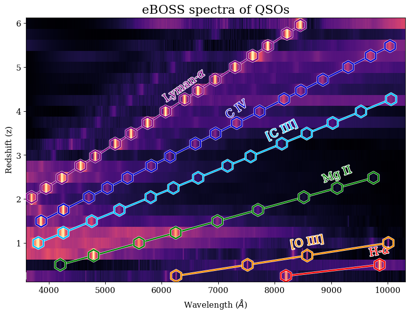
This plot shows 24 different eBOSS spectra in one figure, going from low-reshift (z=0.25) to high-redshift (z=6)! The emission lines are visible in every spectrum, and this figure shows how distance shifts the emissions lines into longer and longer wavelengths! Studying quasars has a broad range of use in astronomical research: because quasars are so luminous, they can be observed at very high redshift and can give scientists insight into distant reaches of the Universe.

---

Searching for High-Redshift JWST spectra

The quasar plot we made with eBOSS spectra is great, but let’s push our quasar sample into even higher redshift quasars by using JWST. JWST is an infrared telescope which observes in longer wavelengths than eBOSS (although there is some overlap between them), making it perfect for observing extremely high redshift galaxies.

Here is a list of three high-redshift QSOs that have been observed with the NIRSPEC instrument, as part of JWST Program GO 1222:

• VDES J0020–3653 (z = 6.860)

• DELS J0411–0907 (z = 6.825)

• UHS J0439+1634 (z = 6.519)

Let’s add these galaxies to our eBOSS plot, to extend our sample to even higher redshift!

# Search for JWST data
jwst_obs_list = Observations.query_criteria(obs_collection='JWST', # Search for JWST data
                                            proposal_id='1222', # Search based on program ID
                                            dataproduct_type='spectrum', # Limit search to spectra
                                            )

# Print lenght of results
print(f"Found {len(jwst_obs_list)} results!")

# Display first 5 results
jwst_obs_list[:5]

Found 238 results!

Table masked=True length=5

intentType	obs_collection	provenance_name	instrument_name	project	filters	wavelength_region	target_name	target_classification	obs_id	s_ra	s_dec	dataproduct_type	proposal_pi	calib_level	t_min	t_max	t_exptime	em_min	em_max	obs_title	t_obs_release	proposal_id	proposal_type	sequence_number	s_region	jpegURL	dataURL	dataRights	mtFlag	srcDen	obsid	objID
str7	str4	str7	str12	str4	str12	str8	str26	str39	str58	float64	float64	str8	str17	int64	float64	float64	float64	float64	float64	str80	float64	str4	str3	int64	str111	str84	str85	str6	bool	float64	str9	str9
science	JWST	CALJWST	NIRSPEC/SLIT	JWST	F170LP;G235H	INFRARED	UHSJ0439+1634	Galaxy; High-redshift galaxies; Quasars	jw01222-o011_s000000001_nirspec_f170lp-g235h-s200a1	69.94621666666667	16.571033333333332	spectrum	Willott, Chris J.	3	59968.23952844908	59968.31842642361	2844.834	1660.0	5000.0	Cosmic reionization, metal enrichment and host galaxies from quasar spectroscopy	60333.76431704	1222	GTO	--	POLYGON 69.945797828 16.571689339 69.946628685 16.571689339 69.946628685 16.570355748 69.945797828 16.570355748	mast:JWST/product/jw01222-o011_s000000001_nirspec_f170lp-g235h-s200a1_cal.jpg	mast:JWST/product/jw01222-o011_s000000001_nirspec_f170lp-g235h-s200a1_s2d.fits	PUBLIC	False	nan	232625998	741717564
science	JWST	CALJWST	NIRSPEC/SLIT	JWST	F070LP;G140H	INFRARED	UHSJ0439+1634	Galaxy; High-redshift galaxies; Quasars	jw01222-o011_s000000012_nirspec_f070lp-g140h-s200a2	69.94621666666667	16.571033333333332	spectrum	Willott, Chris J.	3	59968.23952844908	59968.27992793982	2844.834	700.0	5000.0	Cosmic reionization, metal enrichment and host galaxies from quasar spectroscopy	60333.76431704	1222	GTO	--	POLYGON 69.941442355 16.575358927 69.942289416 16.575358927 69.942289416 16.574003292 69.941442355 16.574003292	mast:JWST/product/jw01222-o011_s000000012_nirspec_f070lp-g140h-s200a2_cal.jpg	mast:JWST/product/jw01222-o011_s000000012_nirspec_f070lp-g140h-s200a2_s2d.fits	PUBLIC	False	nan	232629349	741717578
science	JWST	CALJWST	NIRSPEC/SLIT	JWST	F170LP;G235H	INFRARED	UHSJ0439+1634	Galaxy; High-redshift galaxies; Quasars	jw01222-o011_s000000015_nirspec_f170lp-g235h-s200b1	69.94621666666667	16.571033333333332	spectrum	Willott, Chris J.	3	59968.23952844908	59968.31842642361	2844.834	1660.0	5000.0	Cosmic reionization, metal enrichment and host galaxies from quasar spectroscopy	60333.76431704	1222	GTO	--	POLYGON 69.987084496 16.552858901 69.98791359 16.552858901 69.98791359 16.551496306 69.987084496 16.551496306	mast:JWST/product/jw01222-o011_s000000015_nirspec_f170lp-g235h-s200b1_cal.jpg	mast:JWST/product/jw01222-o011_s000000015_nirspec_f170lp-g235h-s200b1_s2d.fits	PUBLIC	False	nan	232629350	741717587
science	JWST	CALJWST	NIRSPEC/SLIT	JWST	F070LP;G140H	INFRARED	UHSJ0439+1634	Galaxy; High-redshift galaxies; Quasars	jw01222-o011_s000000001_nirspec_f070lp-g140h-s200a1	69.94621666666667	16.571033333333332	spectrum	Willott, Chris J.	3	59968.23952844908	59968.27992793982	2844.834	700.0	5000.0	Cosmic reionization, metal enrichment and host galaxies from quasar spectroscopy	60333.76431704	1222	GTO	--	POLYGON 69.945798319 16.571686993 69.946628519 16.571686993 69.946628519 16.570354577 69.945798319 16.570354577	mast:JWST/product/jw01222-o011_s000000001_nirspec_f070lp-g140h-s200a1_cal.jpg	mast:JWST/product/jw01222-o011_s000000001_nirspec_f070lp-g140h-s200a1_s2d.fits	PUBLIC	False	nan	232625999	741717597
science	JWST	CALJWST	NIRSPEC/SLIT	JWST	F170LP;G235H	INFRARED	UHSJ0439+1634	Galaxy; High-redshift galaxies; Quasars	jw01222-o011_s000000013_nirspec_f170lp-g235h-s400a1	69.94621666666667	16.571033333333332	spectrum	Willott, Chris J.	3	59968.23952844908	59968.31842642361	2844.834	1660.0	5000.0	Cosmic reionization, metal enrichment and host galaxies from quasar spectroscopy	60333.69175919	1222	GTO	--	POLYGON 69.945200123 16.574577994 69.946108378 16.574577994 69.946108378 16.573121456 69.945200123 16.573121456	mast:JWST/product/jw01222-o011_s000000013_nirspec_f170lp-g235h-s400a1_cal.jpg	mast:JWST/product/jw01222-o011_s000000013_nirspec_f170lp-g235h-s400a1_s2d.fits	PUBLIC	False	nan	232626001	741717631

There are a lot of results (over 200!), so for convenience here, let’s just use two files per galaxy, curated in this list below:

# Define a list of JWST spectra to add to our plot
jwst_spectra = [
    {"name": "VDES J0020-3653",
     "proposal_id": 1222,
     "redshift": 6.860,
     "obs1": "jw01222-o012_s000000001_nirspec_f170lp-g235h-s200a2-s200a1",
     "obs2": "jw01222-o012_s000000001_nirspec_f070lp-g140h-s200a1-s200a2"},

    {"name": "DELS J0411-0907",
     "proposal_id": 1222,
     "redshift": 6.825,
     "obs1": "jw01222-o002_s000000001_nirspec_f170lp-g235h-s200a2-s200a1",
     "obs2": "jw01222-o002_s000000001_nirspec_f070lp-g140h-s200a1-s200a2",
     },

    {"name": "UHS J0439+1634",
     "proposal_id": 1222,
     "redshift": 6.519,
     "obs1": "jw01222-o011_s000000001_nirspec_f170lp-g235h-s200a1",
     "obs2": "jw01222-o011_s000000001_nirspec_f070lp-g140h-s200a1",
     },
]

For each of these three galaxies, we will download the JWST spectra and store them in a small dictonary, just like we did for eBOSS.

def get_jwst_qso_spectrum(jwst_spec_dict):
    """
    Given an JWST observation ID, query MAST and download the spectrum using astroquery.mast

    Parameters:
    =============
    jwst_spec_data: dict
        Dictionary of object name and observation ids for retreieving the JWST spectra

    Returns:
    =============
    dictionary of...
    """

    z = jwst_spec_dict['redshift']

    # Query MAST for JWST observation
    obs_list = Observations.query_criteria(obs_collection='JWST', # Search for JWST data
                                           obs_id=jwst_spec_dict['obs1'], # Search on obs_id
                                           )
    # Retrieve products
    products_list = Observations.get_product_list(obs_list)
    # Filter products to just extracted 1D spectra
    products_list = Observations.filter_products(products_list, productType='SCIENCE',
                                                 productSubGroupDescription='ANNNN_X1D',
                                                 mrp_only=True)
    # Download spectrum file
    jwst_manifest = Observations.download_products(products_list)
    # Open file
    jwst_spec = fits.open(jwst_manifest['Local Path'][0])
    # Retrieve wavelength and flux from the file
    wls = jwst_spec['EXTRACT1D'].data['WAVELENGTH']*10000 # convert microns to Angstroms
    observed_flux = jwst_spec['EXTRACT1D'].data['FLUX']
    # Normalize the Flux values based on some percentile values
    min_flux = np.nanpercentile(observed_flux, 5) # 5th percentile
    max_flux = np.nanpercentile(observed_flux, 99.5) # 99th percentile
    normalized_flux = (observed_flux-min_flux)/(max_flux-min_flux)

    # Do it again for the second obs
    obs_list = Observations.query_criteria(obs_collection='JWST', # Search for JWST data
                                           obs_id=jwst_spec_dict['obs2']) # Search on obs_id
    # Retrieve products
    products_list = Observations.get_product_list(obs_list)
    # Filter products to just extracted 1D spectra
    products_list = Observations.filter_products(products_list, productType='SCIENCE',
                                                 productSubGroupDescription='ANNNN_X1D',
                                                 mrp_only=True)
    # Download spectrum file
    jwst_manifest = Observations.download_products(products_list)
    # Open file
    jwst_spec = fits.open(jwst_manifest['Local Path'][0])
    # Retrieve wavelength and flux from the file
    wls = np.append(wls, jwst_spec['EXTRACT1D'].data['WAVELENGTH']*10000) # convert microns to Angstroms
    observed_flux = jwst_spec['EXTRACT1D'].data['FLUX']
    # Normalize the Flux values based on some percentile values
    min_flux = np.nanpercentile(observed_flux, 30) # 30th percentile
    max_flux = np.nanpercentile(observed_flux, 99.5) # 99th percentile
    normalized_flux = np.append(normalized_flux, (observed_flux-min_flux)/(max_flux-min_flux))

    # Define a dictionary with the spectrum and other information we want to save
    qso_spec = {
        "name": jwst_spec_dict['name'],
        "redshift": z,
        "wls": wls[np.argsort(wls)],
        "flux": normalized_flux[np.argsort(wls)],
        }

    return qso_spec   


jwst_qsos = [get_jwst_qso_spectrum(j) for j in jwst_spectra]

Downloading URL https://mast.stsci.edu/api/v0.1/Download/file?uri=mast:JWST/product/jw01222-o012_s000000001_nirspec_f170lp-g235h-s200a2-s200a1_x1d.fits to ./mastDownload/JWST/jw01222-o012_s000000001_nirspec_f170lp-g235h-s200a2-s200a1/jw01222-o012_s000000001_nirspec_f170lp-g235h-s200a2-s200a1_x1d.fits ...

 [Done]

Downloading URL https://mast.stsci.edu/api/v0.1/Download/file?uri=mast:JWST/product/jw01222-o012_s000000001_nirspec_f070lp-g140h-s200a1-s200a2_x1d.fits to ./mastDownload/JWST/jw01222-o012_s000000001_nirspec_f070lp-g140h-s200a1-s200a2/jw01222-o012_s000000001_nirspec_f070lp-g140h-s200a1-s200a2_x1d.fits ...

 [Done]

Downloading URL https://mast.stsci.edu/api/v0.1/Download/file?uri=mast:JWST/product/jw01222-o002_s000000001_nirspec_f170lp-g235h-s200a2-s200a1_x1d.fits to ./mastDownload/JWST/jw01222-o002_s000000001_nirspec_f170lp-g235h-s200a2-s200a1/jw01222-o002_s000000001_nirspec_f170lp-g235h-s200a2-s200a1_x1d.fits ...

 [Done]

Downloading URL https://mast.stsci.edu/api/v0.1/Download/file?uri=mast:JWST/product/jw01222-o002_s000000001_nirspec_f070lp-g140h-s200a1-s200a2_x1d.fits to ./mastDownload/JWST/jw01222-o002_s000000001_nirspec_f070lp-g140h-s200a1-s200a2/jw01222-o002_s000000001_nirspec_f070lp-g140h-s200a1-s200a2_x1d.fits ...

 [Done]

Downloading URL https://mast.stsci.edu/api/v0.1/Download/file?uri=mast:JWST/product/jw01222-o011_s000000001_nirspec_f170lp-g235h-s200a1_x1d.fits to ./mastDownload/JWST/jw01222-o011_s000000001_nirspec_f170lp-g235h-s200a1/jw01222-o011_s000000001_nirspec_f170lp-g235h-s200a1_x1d.fits ...

 [Done]

Downloading URL https://mast.stsci.edu/api/v0.1/Download/file?uri=mast:JWST/product/jw01222-o011_s000000001_nirspec_f070lp-g140h-s200a1_x1d.fits to ./mastDownload/JWST/jw01222-o011_s000000001_nirspec_f070lp-g140h-s200a1/jw01222-o011_s000000001_nirspec_f070lp-g140h-s200a1_x1d.fits ...

 [Done]

Let’s plot one of these, like we did before, to see what it looks like:

# Set up spectrum plot
fig = plt.figure(figsize=(15, 5))
ax1 = plt.subplot2grid((5, 1), (0, 0), colspan=1, rowspan=4)
ax2 = plt.subplot2grid((5, 1), (4, 0), colspan=1, rowspan=1)

qso = jwst_qsos[0]

redshift = qso['redshift']
# Plot the observed spectrum
wls = qso['wls']
flux = qso['flux']
ax1.plot(wls, flux, c='gray', label='Observed Spectrum')

ax2.pcolormesh(wls, [0, 1], [flux, flux],
               cmap='magma', vmin=0, vmax=1)

# Plot emission lines
plot_emission_lines(ax1, redshift)

# Set title and labels
ax1.set_title(f"JWST Spectrum - {qso['name']}")
# Add redshift to plot
ax1.text(0.02, 0.95, f"z = {str(round(redshift, 2))}", 
         fontsize=24, ha='left', va='top', transform=ax1.transAxes)
ax2.set_xlabel(r'Wavelength [$\AA$]')
ax2.set_yticks([])
ax1.set_ylabel('Flux')
ax1.grid() # Add grid lines
ax1.legend(loc='upper right') # Add plot legend
# Set axes limits
ax1.set_xlim(np.min(qso['wls']), np.max(qso['wls']))
ax2.set_xlim(np.min(qso['wls']), np.max(qso['wls']))
ax1.set_ylim(0, 1.1)
plt.subplots_adjust(hspace=0) # remove space between plots

plt.show() # Display Plot

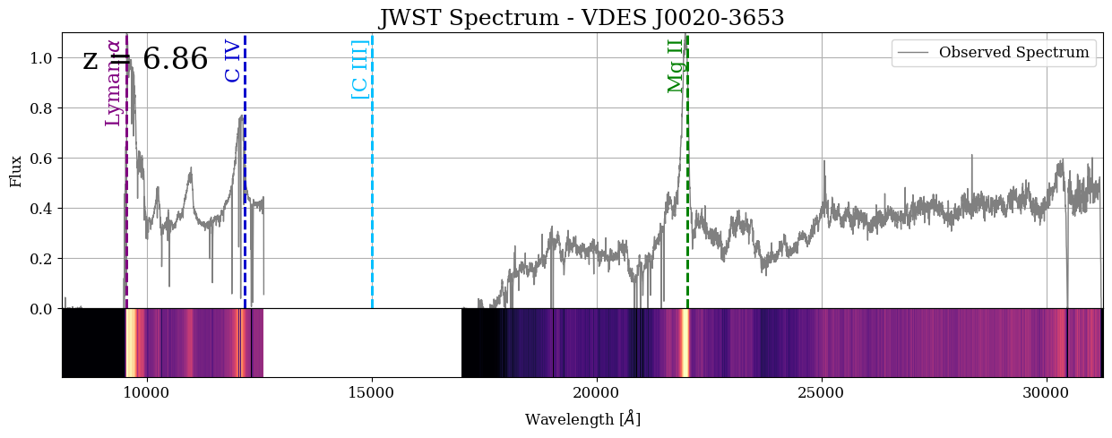
Notice how this NIRSPEC spectrum covers a much different wavelength range than eBOSS. eBOSS spectra fall between 3,000 and 10,000 angstroms in visible light. JWST observed between 7,000 and 30,000 Angstroms! The JWST spectrum still has the same strong emission lines (Lyman-\(\alpha\), C-IV and Mg II) that we saw before in the lower-redshift eBOSS quasars, only in infrared wavelengths because this quasar is so far away.

Combining eBOSS and JWST Data

Now we can recreate our plot from before, adding these JWST spectra as very-high-redshift examples!

fig = plt.figure(figsize=(10, 7))
ax = plt.subplot2grid((1, 1), (0, 0))

for qso in jwst_qsos:
    # Round to nearest 0.25 in redshift just to align things on a grid
    nearest_redshift = round(qso['redshift']*4+0.1)/4
    plt.pcolormesh(qso['wls'], [nearest_redshift-0.07, nearest_redshift+0.07],
                   [qso['flux'], qso['flux']], cmap='magma', vmin=0, vmax=1)
    plt.text(np.min(qso['wls']-100), nearest_redshift, f"JWST {qso['name']}", va='center', ha='right', fontsize=8)


for qso in all_qsos:
    # Round to nearest 0.25 in redshift just to align things on a grid
    nearest_redshift = round(qso['redshift']*4)/4
    plt.pcolormesh(qso['wls'], [nearest_redshift-0.07, nearest_redshift+0.07],
                   [qso['flux'], qso['flux']], cmap='magma', vmin=0, vmax=1)
    plt.text(10400, nearest_redshift, qso["name"], va='center', ha='left', fontsize=8)

all_redshifts = np.array([qso['redshift'] for qso in all_qsos+jwst_qsos])
wl_limits = np.array([np.max(qso['wls']) for qso in all_qsos+jwst_qsos])
wl_limits[wl_limits > 12500] = 12500

# Label and annotate emission lines
for i, emline in enumerate(emission_line_list):
    # Calculate observed wavelength for redshift
    wavelength_obs = (1+all_redshifts)*emline['rest_wavelength']
    # Limit the points to those within the wavelength range of each spectrum
    point_mask = (wavelength_obs <= wl_limits) & (wavelength_obs >= 3500)
    # Plot the points
    points = plt.scatter(wavelength_obs[point_mask], [round(z*4+0.1)/4 for z in all_redshifts[point_mask]],
                         lw=1, edgecolor=emline['label_color'],
                         marker='h', s=300, facecolor='None', zorder=2)
    points.set_path_effects([path_effects.withStroke(linewidth=2, foreground='w')])
    # Add connecting lines between the points
    for i in range(len(wavelength_obs[point_mask])-1):
        cp = ConnectionPatch((wavelength_obs[point_mask][i], all_redshifts[point_mask][i]),
                             (wavelength_obs[point_mask][i+1], all_redshifts[point_mask][i+1]), 
                             coordsA='data', coordsB='data', axesA=ax, axesB=ax,
                             color=emline['label_color'], shrinkA=10, shrinkB=10,
                             linewidth=1, zorder=1)
        cp.set_path_effects([path_effects.withStroke(linewidth=2, foreground='w')])
        ax.add_patch(cp)

    # Add text for line labels
    text_coord_x = wavelength_obs[emline['label_index']]-550
    text_coord_y = all_redshifts[emline['label_index']]+0.075
    text = plt.text(text_coord_x, text_coord_y, emline['emline'],
                    c=emline['label_color'], ha='center', va='center',
                    fontsize=16, rotation=emline['label_angle'])
    # Add white border for readability
    text.set_path_effects([path_effects.withStroke(linewidth=2, foreground='w')])

#plt.xlim(3596, 24000)
plt.xlim(3596, 12500)
plt.ylabel('Redshift (z)')
plt.xlabel(r'Wavelength ($\AA$)')
plt.title('Quasar Emission Lines Across Redshift - JWST and eBOSS')

plt.show()

---

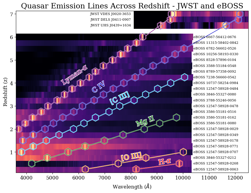
Congratulations! You have reached the end of this tutorial notebook. You have learned how to access and download eBOSS data from MAST, and combine it with NIRSPEC observations to characterize quasar spectra across cosmic time.

Additional Resources

Additional resources are linked below:

• SDSS Legacy Archive at MAST

• SDSS Legacy Archive at MAST User Manual

• SDSS-IV eBOSS Survey

• astroquery.mast User Manual

• MAST API

Citations

If you use eBOSS data for published research, see the following links for information on which citations to include in your paper:

• Citing SDSS

• Citing MAST

• Citing astropy

About this Notebook

Author(s): Julie Imig (jimig@stsci.edu)
Keyword(s): Tutorial, SDSS, eBOSS, JWST, QSO, quasar
First published: March 2025
Last updated: March 2025

---

Top of Page