
Photometry with JWST - Jdaviz#
Author: Camilla Pacifici, Space Telescope Science Institute (adapting notebook by Clare Shanahan)
Date last modified: 2026-04-22, update for Jdaviz version 5.0.0
Tutorial Overview#
This tutorial will demonstrate how to use Jdaviz to support a photometry workflow.
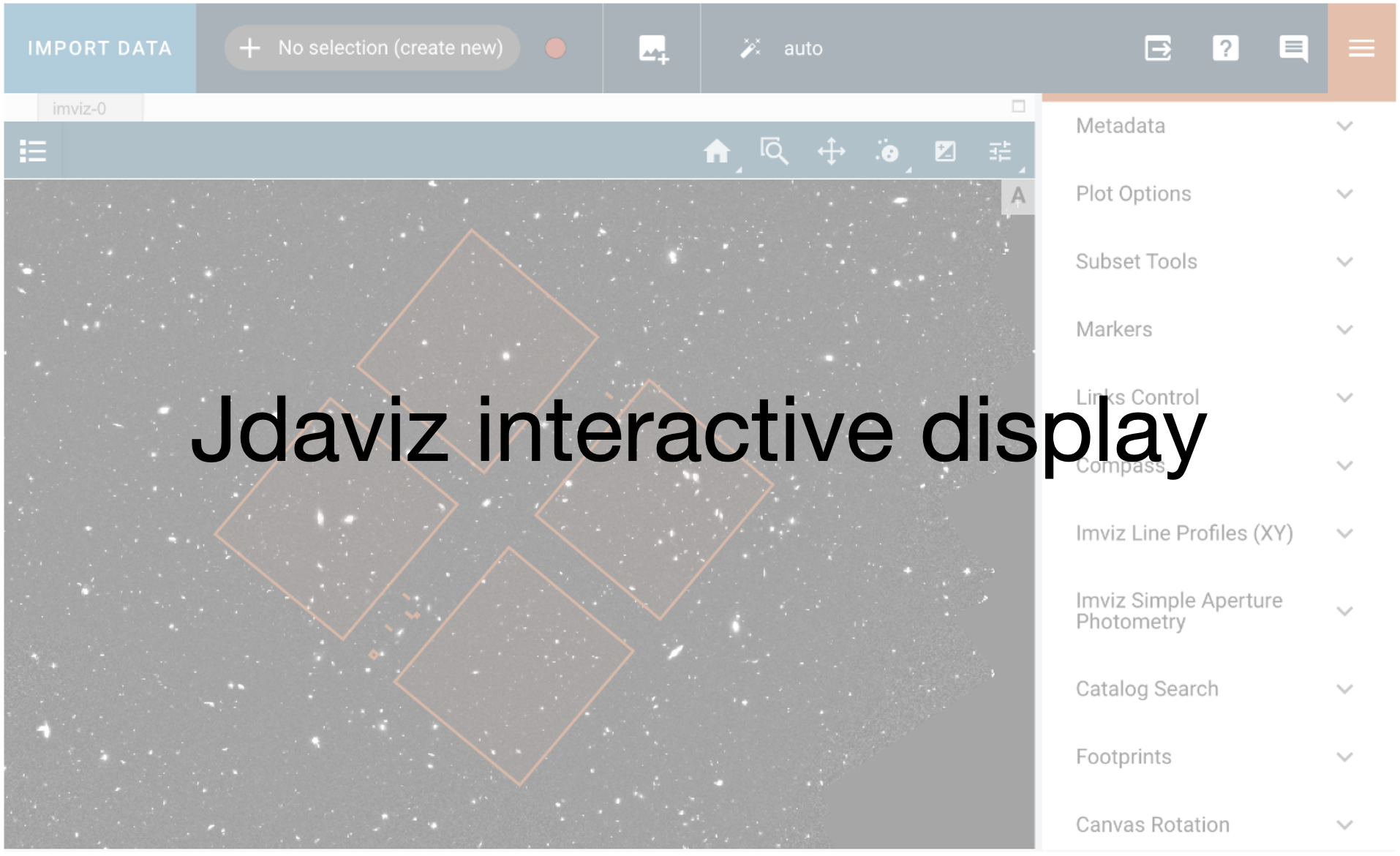
Start Jdaviz and load data.
Setting display options.
Aligning images by WCS.
Load catalog of sources from the interface and from the notebook.
Load footprints.
Select a source and do aperture photometry.
The first half of the tutorial will show you how to perform these tasks in the interface. In the second part, we will see how the same tasks can be performed with code in the notebook.
Import packages#
First, import astroquery for downloading the data, jdaviz, and a few astropy tools.
import os
import subprocess
from astroquery.mast import Observations
import jdaviz as jd
from astropy.table import QTable
from astropy import units as u
from regions import Regions, CircleSkyRegion
def download_files(files_to_download):
"""Download a list of files from MAST.
Parameters
----------
files_to_download : list
List of filenames
"""
for file in files_to_download:
# Check if the file already exists in the current working directory
if os.path.exists(file):
print(f"File {file} already exists. Skipping download.")
continue
cal_uri = f'mast:HLSP/ceers/nircam/{file}.gz'
Observations.download_file(cal_uri)
command = ['gunzip', file, '.gz']
subprocess.run(command, capture_output=True, text=True)
Initialize Viewer#
jd.show()
Loading Data#
Jdaviz can ingest FITS files, ASDF files, or numpy arrays (see documentation for importing data). Here, we will work with standard FITS files provided by the ERS CEERS team as high level data products.
Jdaviz can read either a file path or directly a URI from MAST. Although these data products are available in MAST, we will pull them from a shared space in the platform where they have already being downloaded so we do not have to wait for the download to happen. These files are pretty big!
We will work with three images of the same field in four different filters (F200W, F356W, and F444W) obtained with the NIRCam instrument on JWST.
filenames = ['hlsp_ceers_jwst_nircam_nircam2_f200w_v0.5_i2d.fits',
'hlsp_ceers_jwst_nircam_nircam2_f356w_v0.5_i2d.fits',
'hlsp_ceers_jwst_nircam_nircam2_f444w_v0.5_i2d.fits']
download_files(filenames)
Downloading URL https://mast.stsci.edu/api/v0.1/Download/file?uri=mast:HLSP/ceers/nircam/hlsp_ceers_jwst_nircam_nircam2_f200w_v0.5_i2d.fits.gz to hlsp_ceers_jwst_nircam_nircam2_f200w_v0.5_i2d.fits.gz ...
[Done]
Downloading URL https://mast.stsci.edu/api/v0.1/Download/file?uri=mast:HLSP/ceers/nircam/hlsp_ceers_jwst_nircam_nircam2_f356w_v0.5_i2d.fits.gz to hlsp_ceers_jwst_nircam_nircam2_f356w_v0.5_i2d.fits.gz ...
[Done]
Downloading URL https://mast.stsci.edu/api/v0.1/Download/file?uri=mast:HLSP/ceers/nircam/hlsp_ceers_jwst_nircam_nircam2_f444w_v0.5_i2d.fits.gz to hlsp_ceers_jwst_nircam_nircam2_f444w_v0.5_i2d.fits.gz ...
[Done]
with jd.batch_load(): # not necessary, but this context manager makes loading multiple files more efficient
for filename in filenames:
jd.load(filename, format='Image')
The datasets (given default labels ‘A’, ‘B’, and ‘C’) are loaded into the same viewer. They appear in the data menu on the right hand side. You can select/deselect loaded data to display, remove/re-add data from the viewer, and delete loaded data from the app. To blink between images, press the ‘b’ key (note that blinking will de-select non active layers).
Linking by WCS#
By default, images are pixel linked when loaded. We can link them by WCS in the ‘Orientation’ plugin. This is important for catalog functionality. We can also access the Orientation plugin in coding.
plg_orient = jd.plugins['Orientation']
plg_orient.align_by = "WCS"
/home/runner/micromamba/envs/ci-env/lib/python3.11/site-packages/jdaviz/configs/imviz/wcs_utils.py:566: UserWarning: WCS fiducial coordinates not inside bounding box
warnings.warn("WCS fiducial coordinates not inside bounding box")
Modifying Image Display Options#
Now, we will modify some of the display options to better suit our data. For the live demo, we will do this in the UI in the ‘Plot Options’ plugin by modifying the image stretch from linear to logarithmic, and setting vmax to a more appropriate value. We will make use of ‘layer multiselect’ to apply these options to all images at the same time, but you can set different display options for each image independently as well. The following cell accomplishes the same task from the API.
First, we can check what choices are available for two example options and what is currently set.
plg_plot = jd.plugins['Plot Options']
print(plg_plot.stretch_function.choices)
print(plg_plot.stretch_function.value)
print()
print(plg_plot.image_colormap.choices)
print(plg_plot.image_colormap.value)
['Linear', 'Square Root', 'Arcsinh', 'Logarithmic', 'Spline', 'DQ']
linear
['Gray', 'Viridis', 'Plasma', 'Inferno', 'Magma', 'Purple-Blue', 'Yellow-Green-Blue', 'Yellow-Orange-Red', 'Red-Purple', 'Blue-Green', 'Hot', 'Red-Blue', 'Red-Yellow-Blue', 'Purple-Orange', 'Purple-Green', 'Rainbow', 'Seismic', 'Reversed: Gray', 'Reversed: Viridis', 'Reversed: Plasma', 'Reversed: Inferno', 'Reversed: Magma', 'Reversed: Hot', 'Reversed: Rainbow', 'Random']
gray
# the following code is the API equivalent to the series of UI clicks we will do in the live demo
# get the 'Plot Options' plugin
plg_plot = jd.plugins['Plot Options']
# enable mutiselect so our chosen options are applied to all images
plg_plot.layer.multiselect = True
plg_plot.select_all()
# switch stretch function from default linear to log
plg_plot.stretch_function = 'Logarithmic'
# use the 99.5% stretch function preset
# plg_plot.stretch_preset = '99.5%'
# increase vmax to a more suitable value
plg_plot.stretch_vmax = 0.5
plg_plot.stretch_vmin = 0
Now that we know how to set our own plot options, let’s use one of the RGB presets, just for fun. This will apply preset color, stretch, and opacity settings to each layer.
plg_plot = jd.plugins['Plot Options']
plg_plot.image_color_mode = 'Color'
plg_plot.apply_RGB_presets()
Loading Catalogs#
SDSS and Gaia catalogs can be loaded directly from jdaviz (with more catalog support planned in the future). Additionally, you can load your own catalog into the application.
We will use a portion of one of the catalogs generated in the Photutils demo. The Catalog Search plugin documentation explains how the file needs to be formatted.
# We will need the catalog later so we load it here
catalog_file = 'photutils_cat.ecsv'
cat = QTable.read(catalog_file)
# cat
plg_cat = jd.plugins['Catalog Search']
# Import the catalog
plg_cat.import_catalog(catalog_file)
Loading Regions#
Regions can also be loaded either as Subsets or as Footprints. Subsets are used for analysis and are linked to the datasets so they take some memory. Footprints are just for visual purposes and are much lighter on the tool. Here we load regions created in the Photutils demo as Footprints using the Footprint plugin.
# Get the regions file
region_file = 'kron_apertures.reg'
# Open it with the Regions package
regions = Regions.read(region_file)
# Open the footprint plugin
plg_fprint = jd.plugins['Footprints']
plg_fprint.open_in_tray()
plg_fprint.keep_active = True
# Add the desired overlay
plg_fprint.add_overlay('Kron regions')
# Import the regions
plg_fprint.import_region(regions)
Load instrument footprints#
The Footprint plugin can also be used to load Instruments footprints from JWST and Roman.
# Open the footprint plugin
plg_fprint = jd.plugins['Footprints']
plg_fprint.open_in_tray()
plg_fprint.keep_active = True
# Add a NIRSpec overlay
plg_fprint.add_overlay('nirspec')
# Choose the preset footprint for NIRSpec
plg_fprint.preset = 'NIRSpec'
# Change the center and angle of the footprint
plg_fprint.ra = cat['sky_centroid'][0].ra.value
plg_fprint.dec = cat['sky_centroid'][0].dec.value
plg_fprint.pa = 30
Aperture photometry#
We can do Aperture Photometry in Jdaviz. We will do it on a single source selected from the catalog. We can draw a circular subset near the souce, then use recenter to centroid the position a little better.
Creating and loading regions#
# get the 'Subsets Tools' plugin where we can create and interact with spatial regions in Jdaviz
plg_subset = jd.plugins['Subset Tools']
# Create a circular region around a random source
# This will create a red circular region around a source in the center of the 4 NIRCam detector footprints
circular_region = CircleSkyRegion(center=cat['sky_centroid'][250], radius=3*u.arcsec)
plg_subset.import_region(circular_region)
Aperture Photometry#
With a subset created and placed on one of the sources in the image, we can use the Aperture Photometry plugin to do some analysis. We can make use of ‘batch mode’ to get photometry for all loaded images using the same subset (which is useful when images are well aligned). The API for this is not exposed yet, so we will do it only in UI and we will just get the table of results our here.
# get the plugin
aperture_photometry = jd.plugins['Aperture Photometry']
# export the table of results
aperture_photometry.export_table()