
Creating a Color-Magnitude Diagram for Messier 13#
Learning Goals#
By the end of this tutorial, you will:
Understand how to use
astroquery.mastto download the SDSS Legacy Imaging Survey Data from the MAST archive.Plot a Color-Magnitude Diagram of Messier 13
Calculate the distance to Messier 13 using the Gaia catalog
Approximate the age of Messier 13 using stellar isochrones
Table of Contents#
Introduction#
The Hertzsprung-Russell (HR) Diagram was independently discovered by Ejnar Hertzsprung and Henry Norris Russell in the early 20th century. This diagram effectively plots a star’s theoretical luminosity against its temperature. By examining the position of stars on the HR diagram, we can infer stellar properties such as age, metallicity, or mass. An HR Diagram is also useful for tracking the life cycle of stars. Stars in their hydrogen-core burning phases evolve leftwards on the HR diagram. Eventually, they leave the main sequence to start their red giant phases and move upwards as they begin burning helium in their cores [1].
An observational variation of the HR Diagram is the Color-Magnitude Diagram (CMD), which uses color (a proxy for temperature) and magnitude (a proxy for luminosity). We can use photometric data from a star cluster to create a CMD, and then estimate the age by comparing the main sequence tracks and red giant branch to theoretical isochrones — curves that represent stars of the same age but with different masses, mapping their expected positions at various evolutionary stages. For example, an older cluster will have more stars on the red giant branch whereas a younger cluster will have more stars on the main sequence. The transition between the two evolutionary stages, called the Main Sequence Turn-Off, is the key to determining the age of a stellar cluster [2]

Messier 13 (M13) is a globular cluster located in the constellation Hercules [4]. M13 is estimated to contain over 100,000 stars with a total metallicity ([Fe/H]) of approximately -1.33 dex [5]. This is consistent with the ancient stellar populations found in other globular clusters [6].
In this notebook, we’ll estimate the age of M13 using photometric data from the Sloan Digital Sky Survey’s (SDSS) Legacy Imaging Survey and stellar isochrones from the PARSEC database [7]. By plotting isochrone tracks for a range of ages and comparing them to the observed stellar distribution of M13, we can identify the isochrone that best fits the cluster’s data and thereby estimate its age.
Imports#
The main packages and their use-cases in this tutorial are as follows:
numpy to handle array functions
matplotlib.pyplot for plotting data
matplotlib.image for displaying .jpg images
astroquery.mast.Observations to access SDSS data from MAST
astroquery.mast.Catalogs to access data Gaia data from MAST
pandas to handle large data tables
astropy.io.fits for accessing FITS files
%matplotlib inline

import numpy as np
import matplotlib.pyplot as plt
import matplotlib.image as mpimg

from astroquery.mast import Observations
from astroquery.mast import Catalogs
import pandas as pd
import astropy.io.fits as fits
If you’re not sure if you have the required versions of packages installed on your device, you can run the following cell:
with open("requirements.txt") as f:
    print(f"Required packages for this notebook:\n{f.read()}")
Required packages for this notebook:
pandas >= 2.3.0
astroquery >= 0.4.9
matplotlib >= 3.9.1
numpy >= 1.26.4
To ensure these requirements are installed, you can run the following command in the terminal:
pip install -r requirements.txt
Accessing SDSS Legacy Imaging Survey Data from MAST#
The Mikulski Archive for Space Telescopes (MAST) hosts a large array of data from several telescope missions. In this tutorial, we will be specifically focusing on data from the Sloan Digital Sky Survey’s (SDSS) Imaging Survey.
The SDSS Legacy Imaging Survey was the first SDSS survey completed! Beginning in 1998, the SDSS Legacy Imaging Survey captured around 35,000 square degrees of images until 2009, which covers about one-third of the whole sky. To do this, the survey took millions of 10 by 13 arcminute pictures (called “fields”). Not only does the SDSS Legacy Imaging Survey data at MAST provide users with preview images in .jpg format, but it also has photometric data in all five broad band SDSS filters (u, g, r, i, and z). For more information about the data and products from the SDSS Legacy Imaging Survey, you can check out the SDSS Imaging Archive Manual.
Querying SDSS Legacy Imaging Survey#
You can query data from MAST using the website portal. You can also query MAST data in Python using the package astroquery.mast!
We can query all of the SDSS Legacy Imaging data using Observations.query_criteria with provenance_name = "SDSS Legacy Imaging". Since there is a large amount of data in the SDSS Legacy Imaging archive, we can display the first 10 results using the pagesize parameter as well as the page parameter.
# Querying SDSS Legacy Imaging
imaging_data = Observations.query_criteria(
    provenance_name="SDSS Legacy Imaging", pagesize=10, page=1
)

# Display first 10 entries
imaging_data
| intentType | obs_collection | provenance_name | instrument_name | project | filters | wavelength_region | target_name | target_classification | obs_id | s_ra | s_dec | dataproduct_type | proposal_pi | calib_level | t_min | t_max | t_exptime | em_min | em_max | obs_title | t_obs_release | proposal_id | proposal_type | sequence_number | s_region | jpegURL | dataURL | dataRights | mtFlag | srcDen | obsid | objID |
|---|---|---|---|---|---|---|---|---|---|---|---|---|---|---|---|---|---|---|---|---|---|---|---|---|---|---|---|---|---|---|---|---|
| str7 | str4 | str19 | str11 | str4 | str9 | str7 | str13 | str5 | str24 | float64 | float64 | str5 | str18 | int64 | float64 | float64 | float64 | float64 | float64 | str51 | float64 | str3 | str1 | int64 | str196 | str61 | str61 | str6 | bool | float64 | str9 | str9 |
| science | SDSS | SDSS Legacy Imaging | SDSS Camera | SDSS | u;g;r;i;z | OPTICAL | 005314-1-0139 | FIELD | sdss_image_005314-1-0139 | 198.15448695 | 18.3571809894 | image | SDSS Collaboration | 3 | 53500.342730324075 | 53500.34667149834 | 53.907456 | 304.79999999999995 | 1083.3000000000002 | Sloan Digital Sky Survey (SDSS) Legacy Imaging Data | 55571.0 | N/A | -- | -- | POLYGON 198.0593785849033 18.25122189495538 198.07768815055422 18.475717316443244 198.24970302379174 18.46298317319027 198.23117132226085 18.238504271788198 198.0593785849033 18.25122189495538 | mast:SDSS/sdss/imaging/5314/1/139/frame-irg-005314-1-0139.jpg | mast:SDSS/sdss/imaging/5314/1/139/photoObj-005314-1-0139.fits | PUBLIC | False | nan | 295131540 | 872833130 |
| science | SDSS | SDSS Legacy Imaging | SDSS Camera | SDSS | u;g;r;i;z | OPTICAL | 002328-1-0077 | FIELD | sdss_image_002328-1-0077 | 250.531849896 | 36.5546030081 | image | SDSS Collaboration | 3 | 52052.38049456019 | 52052.38443573444 | 53.907456 | 304.79999999999995 | 1083.3000000000002 | Sloan Digital Sky Survey (SDSS) Legacy Imaging Data | 55571.0 | N/A | -- | -- | POLYGON 250.35859561201013 36.5540642416826 250.5849169880205 36.68707104123642 250.7049953700791 36.55482636287762 250.47885415962534 36.422046570943465 250.35859561201013 36.5540642416826 | mast:SDSS/sdss/imaging/2328/1/77/frame-irg-002328-1-0077.jpg | mast:SDSS/sdss/imaging/2328/1/77/photoObj-002328-1-0077.fits | PUBLIC | False | nan | 295131541 | 872833152 |
| science | SDSS | SDSS Legacy Imaging | SDSS Camera | SDSS | u;g;r;i;z | OPTICAL | 005314-1-0140 | FIELD | sdss_image_005314-1-0140 | 198.311708779 | 18.3454703024 | image | SDSS Collaboration | 3 | 53500.34314502315 | 53500.34708608167 | 53.907456 | 304.79999999999995 | 1083.3000000000002 | Sloan Digital Sky Survey (SDSS) Legacy Imaging Data | 55571.0 | N/A | -- | -- | POLYGON 198.21649447511723 18.23959880389709 198.23503057142125 18.464085709326827 198.40703063427154 18.45118481524402 198.38827261630064 18.22671462236494 198.21649447511723 18.23959880389709 | mast:SDSS/sdss/imaging/5314/1/140/frame-irg-005314-1-0140.jpg | mast:SDSS/sdss/imaging/5314/1/140/photoObj-005314-1-0140.fits | PUBLIC | False | nan | 295131542 | 872833353 |
| science | SDSS | SDSS Legacy Imaging | SDSS Camera | SDSS | u;g;r;i;z | OPTICAL | 002328-1-0078 | FIELD | sdss_image_002328-1-0078 | 250.641575802 | 36.4336890977 | image | SDSS Collaboration | 3 | 52052.380909375 | 52052.38485043352 | 53.907456 | 304.79999999999995 | 1083.3000000000002 | Sloan Digital Sky Survey (SDSS) Legacy Imaging Data | 55571.0 | N/A | -- | -- | POLYGON 250.46857394708124 36.433292936339456 250.69477708949267 36.56611004476571 250.81446826187815 36.43377099259526 250.58844552127275 36.30117975030792 250.46857394708124 36.433292936339456 | mast:SDSS/sdss/imaging/2328/1/78/frame-irg-002328-1-0078.jpg | mast:SDSS/sdss/imaging/2328/1/78/photoObj-002328-1-0078.fits | PUBLIC | False | nan | 295131545 | 872833370 |
| science | SDSS | SDSS Legacy Imaging | SDSS Camera | SDSS | u;g;r;i;z | OPTICAL | 006004-5-0115 | FIELD | sdss_image_006004-5-0115 | 132.906178833 | 11.7175095729 | image | SDSS Collaboration | 3 | 53766.33586886574 | 53766.33980992426 | 53.907456 | 304.79999999999995 | 1083.3000000000002 | Sloan Digital Sky Survey (SDSS) Legacy Imaging Data | 55571.0 | N/A | -- | -- | POLYGON 132.8522937544224 11.588689375039344 132.79770068840654 11.807395680832437 132.9601408208703 11.846212829367165 133.01461297991284 11.627475790886205 132.8522937544224 11.588689375039344 | mast:SDSS/sdss/imaging/6004/5/115/frame-irg-006004-5-0115.jpg | mast:SDSS/sdss/imaging/6004/5/115/photoObj-006004-5-0115.fits | PUBLIC | False | nan | 295131538 | 872833551 |
| science | SDSS | SDSS Legacy Imaging | SDSS Camera | SDSS | u;g;r;i;z | OPTICAL | 005390-6-0160 | FIELD | sdss_image_005390-6-0160 | 197.94127969 | 18.2381062174 | image | SDSS Collaboration | 3 | 53527.20246550926 | 53527.20640656778 | 53.907456 | 304.79999999999995 | 1083.3000000000002 | Sloan Digital Sky Survey (SDSS) Legacy Imaging Data | 55571.0 | N/A | -- | -- | POLYGON 197.84741353404715 18.131209786172366 197.86324377011348 18.35587515688674 198.03525345567525 18.344847136688504 198.01920212616727 18.120195981879778 197.84741353404715 18.131209786172366 | mast:SDSS/sdss/imaging/5390/6/160/frame-irg-005390-6-0160.jpg | mast:SDSS/sdss/imaging/5390/6/160/photoObj-005390-6-0160.fits | PUBLIC | False | nan | 295131546 | 872833559 |
| science | SDSS | SDSS Legacy Imaging | SDSS Camera | SDSS | u;g;r;i;z | OPTICAL | 002328-1-0079 | FIELD | sdss_image_002328-1-0079 | 250.750952787 | 36.3126609264 | image | SDSS Collaboration | 3 | 52052.38132395833 | 52052.38526501685 | 53.907456 | 304.79999999999995 | 1083.3000000000002 | Sloan Digital Sky Survey (SDSS) Legacy Imaging Data | 55571.0 | N/A | -- | -- | POLYGON 250.578252364172 36.31247050799863 250.80425448876198 36.44501655574568 250.92354299824817 36.312538406297975 250.69772164198693 36.180216970539945 250.578252364172 36.31247050799863 | mast:SDSS/sdss/imaging/2328/1/79/frame-irg-002328-1-0079.jpg | mast:SDSS/sdss/imaging/2328/1/79/photoObj-002328-1-0079.fits | PUBLIC | False | nan | 295131548 | 872833580 |
| science | SDSS | SDSS Legacy Imaging | SDSS Camera | SDSS | u;g;r;i;z | OPTICAL | 006004-5-0116 | FIELD | sdss_image_006004-5-0116 | 133.054718302 | 11.7529936035 | image | SDSS Collaboration | 3 | 53766.336283449076 | 53766.34022450759 | 53.907456 | 304.79999999999995 | 1083.3000000000002 | Sloan Digital Sky Survey (SDSS) Legacy Imaging Data | 55571.0 | N/A | -- | -- | POLYGON 133.0007716743229 11.624168614910673 132.9462793280331 11.842904879731558 133.1087420057388 11.881701584074037 133.16311301477495 11.662934551585074 133.0007716743229 11.624168614910673 | mast:SDSS/sdss/imaging/6004/5/116/frame-irg-006004-5-0116.jpg | mast:SDSS/sdss/imaging/6004/5/116/photoObj-006004-5-0116.fits | PUBLIC | False | nan | 295131544 | 872833765 |
| science | SDSS | SDSS Legacy Imaging | SDSS Camera | SDSS | u;g;r;i;z | OPTICAL | 005390-6-0161 | FIELD | sdss_image_005390-6-0161 | 198.098496115 | 18.2279588533 | image | SDSS Collaboration | 3 | 53527.20288009259 | 53527.20682126685 | 53.907456 | 304.79999999999995 | 1083.3000000000002 | Sloan Digital Sky Survey (SDSS) Legacy Imaging Data | 55571.0 | N/A | -- | -- | POLYGON 198.00455378404033 18.121124702001982 198.02057283752566 18.345783137587688 198.19254592087316 18.33463744385239 198.1763059825853 18.109993382520553 198.00455378404033 18.121124702001982 | mast:SDSS/sdss/imaging/5390/6/161/frame-irg-005390-6-0161.jpg | mast:SDSS/sdss/imaging/5390/6/161/photoObj-005390-6-0161.fits | PUBLIC | False | nan | 295131549 | 872833771 |
| science | SDSS | SDSS Legacy Imaging | SDSS Camera | SDSS | u;g;r;i;z | OPTICAL | 004879-2-0091 | FIELD | sdss_image_004879-2-0091 | 315.324305613 | 16.2374578257 | image | SDSS Collaboration | 3 | 53291.10557037037 | 53291.10951166037 | 53.907456 | 304.79999999999995 | 1083.3000000000002 | Sloan Digital Sky Survey (SDSS) Legacy Imaging Data | 55571.0 | N/A | -- | -- | POLYGON 315.2814974558859 16.104501914345207 315.2057637623335 16.317537720063836 315.3672086305765 16.370301045582334 315.44278784074857 16.157208035678934 315.2814974558859 16.104501914345207 | mast:SDSS/sdss/imaging/4879/2/91/frame-irg-004879-2-0091.jpg | mast:SDSS/sdss/imaging/4879/2/91/photoObj-004879-2-0091.fits | PUBLIC | False | nan | 295131550 | 872833791 |
The table above provides some basic information for each object:
instrument_name:SDSS Cameraindicates that the imaging data were collected using the SDSS camera.filters: Indicates the SDSS filters used in the survey (u, g, r, i, and z).wavelength_region: Indicates the region of the electromagnetic spectrum observed. This should beOPTICAL, since the SDSS Legacy Imaging Survey observed in the optical wavelength range.target_classification:FIELDindicates the survey captured images of the sky.obs_id: Observation ID associated with the image.s_raands_dec: Right ascension and declination.dataproduct_type: This should beimagesince we’re focusing on an imaging survey.t_minandt_max: The modified Julian dates indicating the start and end times of the exposures.em_minandem_max: The minimum and maximum wavelengths observed by the survey. For the SDSS Legacy Imaging survey, this range is approximately 304.8 - 1083.3 nanometers (optical).
Sampling SDSS Legacy Imaging Survey for M13#
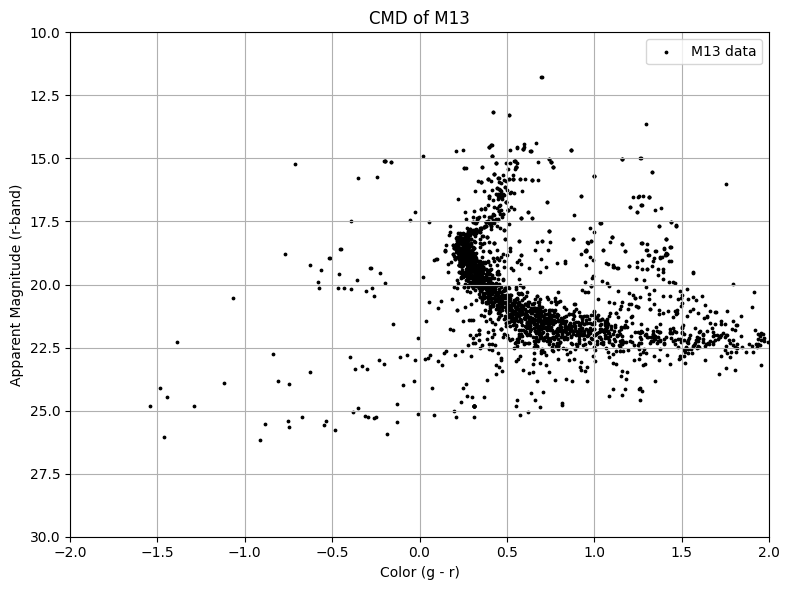
In this tutorial, we will be gathering g-band and r-band magnitudes of stars in M13 measured by the SDSS Legacy Imaging survey by querying and downloading data through MAST. We’ll plot these on a CMD where the apparent r-band magnitude is on the y-axis, and color (g-band minus r-band) is on the x-axis. We’ll later plot this CMD with a CMD of isochrones from the PARSEC database.
For the purpose of this tutorial, we will only focus on querying by object name. We can query the SDSS Legacy Imaging Survey for M13 data using objectname="M13".
# Querying SDSS Legacy Imaging for M13
obs_table = Observations.query_criteria(
    objectname="M13", provenance_name="SDSS Legacy Imaging"
)

# Displaying the table
obs_table
| intentType | obs_collection | provenance_name | instrument_name | project | filters | wavelength_region | target_name | target_classification | obs_id | s_ra | s_dec | dataproduct_type | proposal_pi | calib_level | t_min | t_max | t_exptime | em_min | em_max | obs_title | t_obs_release | proposal_id | proposal_type | sequence_number | s_region | jpegURL | dataURL | dataRights | mtFlag | srcDen | obsid | objID | objID1 | distance |
|---|---|---|---|---|---|---|---|---|---|---|---|---|---|---|---|---|---|---|---|---|---|---|---|---|---|---|---|---|---|---|---|---|---|---|
| str7 | str4 | str19 | str11 | str4 | str9 | str7 | str13 | str5 | str24 | float64 | float64 | str5 | str18 | int64 | float64 | float64 | float64 | float64 | float64 | str51 | float64 | str3 | str1 | int64 | str195 | str61 | str61 | str6 | bool | float64 | str9 | str9 | str9 | float64 |
| science | SDSS | SDSS Legacy Imaging | SDSS Camera | SDSS | u;g;r;i;z | OPTICAL | 002328-1-0077 | FIELD | sdss_image_002328-1-0077 | 250.531849896 | 36.5546030081 | image | SDSS Collaboration | 3 | 52052.38049456019 | 52052.38443573444 | 53.907456 | 304.79999999999995 | 1083.3000000000002 | Sloan Digital Sky Survey (SDSS) Legacy Imaging Data | 55571.0 | N/A | -- | -- | POLYGON 250.35859561201013 36.5540642416826 250.5849169880205 36.68707104123642 250.7049953700791 36.55482636287762 250.47885415962534 36.422046570943465 250.35859561201013 36.5540642416826 | mast:SDSS/sdss/imaging/2328/1/77/frame-irg-002328-1-0077.jpg | mast:SDSS/sdss/imaging/2328/1/77/photoObj-002328-1-0077.fits | PUBLIC | False | nan | 295131541 | 872833152 | 872833152 | 45.926438874565356 |
| science | SDSS | SDSS Legacy Imaging | SDSS Camera | SDSS | u;g;r;i;z | OPTICAL | 002328-1-0078 | FIELD | sdss_image_002328-1-0078 | 250.641575802 | 36.4336890977 | image | SDSS Collaboration | 3 | 52052.380909375 | 52052.38485043352 | 53.907456 | 304.79999999999995 | 1083.3000000000002 | Sloan Digital Sky Survey (SDSS) Legacy Imaging Data | 55571.0 | N/A | -- | -- | POLYGON 250.46857394708124 36.433292936339456 250.69477708949267 36.56611004476571 250.81446826187815 36.43377099259526 250.58844552127275 36.30117975030792 250.46857394708124 36.433292936339456 | mast:SDSS/sdss/imaging/2328/1/78/frame-irg-002328-1-0078.jpg | mast:SDSS/sdss/imaging/2328/1/78/photoObj-002328-1-0078.fits | PUBLIC | False | nan | 295131545 | 872833370 | 872833370 | 165.0330293374257 |
| science | SDSS | SDSS Legacy Imaging | SDSS Camera | SDSS | u;g;r;i;z | OPTICAL | 002328-1-0079 | FIELD | sdss_image_002328-1-0079 | 250.750952787 | 36.3126609264 | image | SDSS Collaboration | 3 | 52052.38132395833 | 52052.38526501685 | 53.907456 | 304.79999999999995 | 1083.3000000000002 | Sloan Digital Sky Survey (SDSS) Legacy Imaging Data | 55571.0 | N/A | -- | -- | POLYGON 250.578252364172 36.31247050799863 250.80425448876198 36.44501655574568 250.92354299824817 36.312538406297975 250.69772164198693 36.180216970539945 250.578252364172 36.31247050799863 | mast:SDSS/sdss/imaging/2328/1/79/frame-irg-002328-1-0079.jpg | mast:SDSS/sdss/imaging/2328/1/79/photoObj-002328-1-0079.fits | PUBLIC | False | nan | 295131548 | 872833580 | 872833580 | 698.8182536420179 |
| science | SDSS | SDSS Legacy Imaging | SDSS Camera | SDSS | u;g;r;i;z | OPTICAL | 003226-5-0126 | FIELD | sdss_image_003226-5-0126 | 250.393866981 | 36.6493290806 | image | SDSS Collaboration | 3 | 52434.38493240741 | 52434.38887323444 | 53.907456 | 304.79999999999995 | 1083.3000000000002 | Sloan Digital Sky Survey (SDSS) Legacy Imaging Data | 55571.0 | N/A | -- | -- | POLYGON 250.22044996940195 36.64428282774371 250.44154003131922 36.7830573250709 250.5671980243839 36.65405635086531 250.34625148107756 36.51551412556894 250.22044996940195 36.64428282774371 | mast:SDSS/sdss/imaging/3226/5/126/frame-irg-003226-5-0126.jpg | mast:SDSS/sdss/imaging/3226/5/126/photoObj-003226-5-0126.fits | PUBLIC | False | nan | 295131553 | 872834007 | 872834007 | 291.37717938143663 |
| science | SDSS | SDSS Legacy Imaging | SDSS Camera | SDSS | u;g;r;i;z | OPTICAL | 003226-5-0127 | FIELD | sdss_image_003226-5-0127 | 250.508705852 | 36.5313775037 | image | SDSS Collaboration | 3 | 52434.38534710648 | 52434.38928770203 | 53.907456 | 304.79999999999995 | 1083.3000000000002 | Sloan Digital Sky Survey (SDSS) Legacy Imaging Data | 55571.0 | N/A | -- | -- | POLYGON 250.33553477042537 36.52648700305302 250.55648135804705 36.66507314658227 250.68179021520078 36.53595013848635 250.46098757081998 36.397595183888505 250.33553477042537 36.52648700305302 | mast:SDSS/sdss/imaging/3226/5/127/frame-irg-003226-5-0127.jpg | mast:SDSS/sdss/imaging/3226/5/127/photoObj-003226-5-0127.fits | PUBLIC | False | nan | 295131557 | 872834246 | 872834246 | 0.0 |
| science | SDSS | SDSS Legacy Imaging | SDSS Camera | SDSS | u;g;r;i;z | OPTICAL | 003226-5-0128 | FIELD | sdss_image_003226-5-0128 | 250.623202081 | 36.4133581779 | image | SDSS Collaboration | 3 | 52434.38576168982 | 52434.38970240111 | 53.907456 | 304.79999999999995 | 1083.3000000000002 | Sloan Digital Sky Survey (SDSS) Legacy Imaging Data | 55571.0 | N/A | -- | -- | POLYGON 250.45026832382496 36.40860979104661 250.67107742007923 36.547001839458886 250.79604843682253 36.417789795153695 250.57538360434452 36.27962787829743 250.45026832382496 36.40860979104661 | mast:SDSS/sdss/imaging/3226/5/128/frame-irg-003226-5-0128.jpg | mast:SDSS/sdss/imaging/3226/5/128/photoObj-003226-5-0128.fits | PUBLIC | False | nan | 295131561 | 872834493 | 872834493 | 197.2958680603298 |
| science | SDSS | SDSS Legacy Imaging | SDSS Camera | SDSS | u;g;r;i;z | OPTICAL | 002328-1-0076 | FIELD | sdss_image_002328-1-0076 | 250.421761559 | 36.6753974425 | image | SDSS Collaboration | 3 | 52052.38007997685 | 52052.38402115111 | 53.907456 | 304.79999999999995 | 1083.3000000000002 | Sloan Digital Sky Survey (SDSS) Legacy Imaging Data | 55571.0 | N/A | -- | -- | POLYGON 250.24825412597377 36.67468245014842 250.47469149264754 36.80794394562259 250.59516092735302 36.67579584579734 250.36890336174514 36.54276250299432 250.24825412597377 36.67468245014842 | mast:SDSS/sdss/imaging/2328/1/76/frame-irg-002328-1-0076.jpg | mast:SDSS/sdss/imaging/2328/1/76/photoObj-002328-1-0076.fits | PUBLIC | False | nan | 295131565 | 872834928 | 872834928 | 333.0209007636813 |
| science | SDSS | SDSS Legacy Imaging | SDSS Camera | SDSS | u;g;r;i;z | OPTICAL | 003225-4-0266 | FIELD | sdss_image_003225-4-0266 | 250.475912605 | 36.2228649182 | image | SDSS Collaboration | 3 | 52434.28733101852 | 52434.291272424256 | 53.907456 | 304.79999999999995 | 1083.3000000000002 | Sloan Digital Sky Survey (SDSS) Legacy Imaging Data | 55571.0 | N/A | -- | -- | POLYGON 250.3035437634285 36.217875087370984 250.52334971401882 36.35664194279063 250.6481953945402 36.22753993420965 250.42853037114884 36.08900145821686 250.3035437634285 36.217875087370984 | mast:SDSS/sdss/imaging/3225/4/266/frame-irg-003225-4-0266.jpg | mast:SDSS/sdss/imaging/3225/4/266/photoObj-003225-4-0266.fits | PUBLIC | False | nan | 297954617 | 881849320 | 881849320 | 475.1195995236801 |
| science | SDSS | SDSS Legacy Imaging | SDSS Camera | SDSS | u;g;r;i;z | OPTICAL | 003225-4-0265 | FIELD | sdss_image_003225-4-0265 | 250.361497186 | 36.340810178 | image | SDSS Collaboration | 3 | 52434.28691631944 | 52434.29085772519 | 53.907456 | 304.79999999999995 | 1083.3000000000002 | Sloan Digital Sky Survey (SDSS) Legacy Imaging Data | 55571.0 | N/A | -- | -- | POLYGON 250.18888442184692 36.33566994315121 250.4088170275986 36.47465028763916 250.53402462257387 36.34563447238449 250.31423253225782 36.20688359738639 250.18888442184692 36.33566994315121 | mast:SDSS/sdss/imaging/3225/4/265/frame-irg-003225-4-0265.jpg | mast:SDSS/sdss/imaging/3225/4/265/photoObj-003225-4-0265.fits | PUBLIC | False | nan | 297954625 | 881849368 | 881849368 | 3.866197461580117 |
| science | SDSS | SDSS Legacy Imaging | SDSS Camera | SDSS | u;g;r;i;z | OPTICAL | 003225-4-0264 | FIELD | sdss_image_003225-4-0264 | 250.246710451 | 36.4586237958 | image | SDSS Collaboration | 3 | 52434.28650173611 | 52434.29044314185 | 53.907456 | 304.79999999999995 | 1083.3000000000002 | Sloan Digital Sky Survey (SDSS) Legacy Imaging Data | 55571.0 | N/A | -- | -- | POLYGON 250.07380618478217 36.45332038759552 250.29390605041334 36.59250454483102 250.4195301652173 36.463610007146634 250.19957027912378 36.32465655078415 250.07380618478217 36.45332038759552 | mast:SDSS/sdss/imaging/3225/4/264/frame-irg-003225-4-0264.jpg | mast:SDSS/sdss/imaging/3225/4/264/photoObj-003225-4-0264.fits | PUBLIC | False | nan | 297955206 | 881852918 | 881852918 | 14.088016661483353 |
| science | SDSS | SDSS Legacy Imaging | SDSS Camera | SDSS | u;g;r;i;z | OPTICAL | 003225-5-0264 | FIELD | sdss_image_003225-5-0264 | 250.658183453 | 36.7170700025 | image | SDSS Collaboration | 3 | 52434.28650173611 | 52434.29044314185 | 53.907456 | 304.79999999999995 | 1083.3000000000002 | Sloan Digital Sky Survey (SDSS) Legacy Imaging Data | 55571.0 | N/A | -- | -- | POLYGON 250.48467210361827 36.712352507710065 250.7062922106185 36.8507365527109 250.8316071569812 36.72146825665738 250.61013383419206 36.58331657086478 250.48467210361827 36.712352507710065 | mast:SDSS/sdss/imaging/3225/5/264/frame-irg-003225-5-0264.jpg | mast:SDSS/sdss/imaging/3225/5/264/photoObj-003225-5-0264.fits | PUBLIC | False | nan | 297956572 | 881861114 | 881861114 | 696.0625286367105 |
| science | SDSS | SDSS Legacy Imaging | SDSS Camera | SDSS | u;g;r;i;z | OPTICAL | 003206-5-0049 | FIELD | sdss_image_003206-5-0049 | 250.612893043 | 36.4240856059 | image | SDSS Collaboration | 3 | 52424.392360763886 | 52424.3963012437 | 53.907456 | 304.79999999999995 | 1083.3000000000002 | Sloan Digital Sky Survey (SDSS) Legacy Imaging Data | 55571.0 | N/A | -- | -- | POLYGON 250.43997310231262 36.41934331740604 250.66076727431061 36.557717739869794 250.78572556890498 36.42851114443372 250.5650757278609 36.29036684119189 250.43997310231262 36.41934331740604 | mast:SDSS/sdss/imaging/3206/5/49/frame-irg-003206-5-0049.jpg | mast:SDSS/sdss/imaging/3206/5/49/photoObj-003206-5-0049.fits | PUBLIC | False | nan | 298315923 | 885161315 | 885161315 | 148.4875090756533 |
| science | SDSS | SDSS Legacy Imaging | SDSS Camera | SDSS | u;g;r;i;z | OPTICAL | 003225-4-0263 | FIELD | sdss_image_003225-4-0263 | 250.131581565 | 36.5763631387 | image | SDSS Collaboration | 3 | 52434.2860869213 | 52434.290028327036 | 53.907456 | 304.79999999999995 | 1083.3000000000002 | Sloan Digital Sky Survey (SDSS) Legacy Imaging Data | 55571.0 | N/A | -- | -- | POLYGON 249.9584663869535 36.57087345241625 250.17866018972612 36.7102635461507 250.30461310469724 36.58153460434509 250.08455864103615 36.442376203777485 249.9584663869535 36.57087345241625 | mast:SDSS/sdss/imaging/3225/4/263/frame-irg-003225-4-0263.jpg | mast:SDSS/sdss/imaging/3225/4/263/photoObj-003225-4-0263.fits | PUBLIC | False | nan | 297954450 | 881848318 | 881848318 | 552.7628408052574 |
| science | SDSS | SDSS Legacy Imaging | SDSS Camera | SDSS | u;g;r;i;z | OPTICAL | 003225-5-0265 | FIELD | sdss_image_003225-5-0265 | 250.772697343 | 36.5988511392 | image | SDSS Collaboration | 3 | 52434.28691631944 | 52434.29085772519 | 53.907456 | 304.79999999999995 | 1083.3000000000002 | Sloan Digital Sky Survey (SDSS) Legacy Imaging Data | 55571.0 | N/A | -- | -- | POLYGON 250.59946781174085 36.59430692699014 250.82094276799123 36.732493216455595 250.945838402895 36.603077335526315 250.72451085188032 36.46512219070452 250.59946781174085 36.59430692699014 | mast:SDSS/sdss/imaging/3225/5/265/frame-irg-003225-5-0265.jpg | mast:SDSS/sdss/imaging/3225/5/265/photoObj-003225-5-0265.fits | PUBLIC | False | nan | 297955991 | 881857628 | 881857628 | 695.9044368869569 |
| science | SDSS | SDSS Legacy Imaging | SDSS Camera | SDSS | u;g;r;i;z | OPTICAL | 003206-5-0048 | FIELD | sdss_image_003206-5-0048 | 250.498361731 | 36.5421282405 | image | SDSS Collaboration | 3 | 52424.39194606482 | 52424.39588677611 | 53.907456 | 304.79999999999995 | 1083.3000000000002 | Sloan Digital Sky Survey (SDSS) Legacy Imaging Data | 55571.0 | N/A | -- | -- | POLYGON 250.3251783392619 36.53722296813955 250.5460945557796 36.67581178341232 250.67145849499735 36.54671558141969 250.4506860481943 36.408358051183676 250.3251783392619 36.53722296813955 | mast:SDSS/sdss/imaging/3206/5/48/frame-irg-003206-5-0048.jpg | mast:SDSS/sdss/imaging/3206/5/48/photoObj-003206-5-0048.fits | PUBLIC | False | nan | 298315544 | 885157501 | 885157501 | 0.0 |
| science | SDSS | SDSS Legacy Imaging | SDSS Camera | SDSS | u;g;r;i;z | OPTICAL | 003206-5-0050 | FIELD | sdss_image_003206-5-0050 | 250.727105633 | 36.3059574758 | image | SDSS Collaboration | 3 | 52424.392775231485 | 52424.39671629 | 53.907456 | 304.79999999999995 | 1083.3000000000002 | Sloan Digital Sky Survey (SDSS) Legacy Imaging Data | 55571.0 | N/A | -- | -- | POLYGON 250.55442273973065 36.301364449432214 250.77506303756408 36.43955055679796 250.89970041241125 36.31023484630317 250.67920474779717 36.172277813761866 250.55442273973065 36.301364449432214 | mast:SDSS/sdss/imaging/3206/5/50/frame-irg-003206-5-0050.jpg | mast:SDSS/sdss/imaging/3206/5/50/photoObj-003206-5-0050.fits | PUBLIC | False | nan | 298315811 | 885160096 | 885160096 | 687.4444027605829 |
| science | SDSS | SDSS Legacy Imaging | SDSS Camera | SDSS | u;g;r;i;z | OPTICAL | 003206-5-0047 | FIELD | sdss_image_003206-5-0047 | 250.383483804 | 36.6600485065 | image | SDSS Collaboration | 3 | 52424.39153148148 | 52424.395472077034 | 53.907456 | 304.79999999999995 | 1083.3000000000002 | Sloan Digital Sky Survey (SDSS) Legacy Imaging Data | 55571.0 | N/A | -- | -- | POLYGON 250.21006556260414 36.65497749936012 250.43111640889498 36.79378288075555 250.55681621645243 36.66480048402042 250.33590870037474 36.526227436667 250.21006556260414 36.65497749936012 | mast:SDSS/sdss/imaging/3206/5/47/frame-irg-003206-5-0047.jpg | mast:SDSS/sdss/imaging/3206/5/47/photoObj-003206-5-0047.fits | PUBLIC | False | nan | 298315987 | 885162046 | 885162046 | 340.1997581534808 |
From the query results, we can see that there are 17 SDSS fields that cover M13! The distance column shows how far each field is from the center of the cluster in arcseconds.
Downloading SDSS Legacy Imaging Survey Data Products#
For each image, there are 7 available products: The preview .jpg image, the FITS files in each respective SDSS filter (u, g, r, i, and z), and the full FITS file with all five filters combined. The full FITS file is listed as SDSS Imaging Catalogs for the productSubGroupDescription parameter.
For more information about products available at MAST, you can check out the SDSS Legacy Imaging Survey Documentation.
# Viewing available products
products = Observations.get_product_list(obs_table)
products
| obsID | obs_collection | dataproduct_type | obs_id | description | type | dataURI | productType | productGroupDescription | productSubGroupDescription | productDocumentationURL | project | prvversion | proposal_id | productFilename | size | parent_obsid | dataRights | calib_level | filters |
|---|---|---|---|---|---|---|---|---|---|---|---|---|---|---|---|---|---|---|---|
| str9 | str4 | str12 | str28 | str246 | str1 | str64 | str7 | str28 | str21 | str70 | str19 | str3 | str3 | str30 | int64 | str9 | str6 | int64 | str9 |
| 295131541 | SDSS | image | sdss_image_002328-1-0077 | Preview-Full | S | mast:SDSS/sdss/imaging/2328/1/77/frame-irg-002328-1-0077.jpg | PREVIEW | -- | -- | -- | SDSS Legacy Imaging | DR8 | N/A | frame-irg-002328-1-0077.jpg | 1195118 | 295131541 | PUBLIC | 3 | u;g;r;i;z |
| 295131541 | SDSS | image | sdss_image_002328-1-0077 | SDSS calibrated, sky-subtracted corrected photometry frame and associated calibration metadata for each run number, camera column, and field name within SDSS. | S | mast:SDSS/sdss/imaging/2328/1/77/frame-g-002328-1-0077.fits.bz2 | SCIENCE | Minimum Recommended Products | IMAGE | https://outerspace.stsci.edu/display/SDSS/Legacy+Imaging+Data+Products | SDSS Legacy Imaging | DR8 | N/A | frame-g-002328-1-0077.fits.bz2 | 3466198 | 295131541 | PUBLIC | 2 | g |
| 295131541 | SDSS | image | sdss_image_002328-1-0077 | SDSS calibrated, sky-subtracted corrected photometry frame and associated calibration metadata for each run number, camera column, and field name within SDSS. | S | mast:SDSS/sdss/imaging/2328/1/77/frame-i-002328-1-0077.fits.bz2 | SCIENCE | Minimum Recommended Products | IMAGE | https://outerspace.stsci.edu/display/SDSS/Legacy+Imaging+Data+Products | SDSS Legacy Imaging | DR8 | N/A | frame-i-002328-1-0077.fits.bz2 | 3731895 | 295131541 | PUBLIC | 2 | i |
| 295131541 | SDSS | image | sdss_image_002328-1-0077 | SDSS calibrated, sky-subtracted corrected photometry frame and associated calibration metadata for each run number, camera column, and field name within SDSS. | S | mast:SDSS/sdss/imaging/2328/1/77/frame-r-002328-1-0077.fits.bz2 | SCIENCE | Minimum Recommended Products | IMAGE | https://outerspace.stsci.edu/display/SDSS/Legacy+Imaging+Data+Products | SDSS Legacy Imaging | DR8 | N/A | frame-r-002328-1-0077.fits.bz2 | 3206091 | 295131541 | PUBLIC | 2 | r |
| 295131541 | SDSS | image | sdss_image_002328-1-0077 | SDSS calibrated, sky-subtracted corrected photometry frame and associated calibration metadata for each run number, camera column, and field name within SDSS. | S | mast:SDSS/sdss/imaging/2328/1/77/frame-u-002328-1-0077.fits.bz2 | SCIENCE | Minimum Recommended Products | IMAGE | https://outerspace.stsci.edu/display/SDSS/Legacy+Imaging+Data+Products | SDSS Legacy Imaging | DR8 | N/A | frame-u-002328-1-0077.fits.bz2 | 3331655 | 295131541 | PUBLIC | 2 | u |
| 295131541 | SDSS | image | sdss_image_002328-1-0077 | SDSS calibrated, sky-subtracted corrected photometry frame and associated calibration metadata for each run number, camera column, and field name within SDSS. | S | mast:SDSS/sdss/imaging/2328/1/77/frame-z-002328-1-0077.fits.bz2 | SCIENCE | Minimum Recommended Products | IMAGE | https://outerspace.stsci.edu/display/SDSS/Legacy+Imaging+Data+Products | SDSS Legacy Imaging | DR8 | N/A | frame-z-002328-1-0077.fits.bz2 | 3077494 | 295131541 | PUBLIC | 2 | z |
| 295131541 | SDSS | image | sdss_image_002328-1-0077 | SDSS Legacy Imaging photoObj catalog. This contains the full, calibrated outputs of the SDSS Imaging Pipeline including source detection, classification, magnitude measurements, and quality flags for each field and all five filters in that field. | S | mast:SDSS/sdss/imaging/2328/1/77/photoObj-002328-1-0077.fits | SCIENCE | Minimum Recommended Products | SDSS Imaging Catalogs | https://outerspace.stsci.edu/display/SDSS/Legacy+Imaging+Data+Products | SDSS Legacy Imaging | DR8 | N/A | photoObj-002328-1-0077.fits | 8640 | 295131541 | PUBLIC | 3 | u;g;r;i;z |
| 295131545 | SDSS | image | sdss_image_002328-1-0078 | Preview-Full | S | mast:SDSS/sdss/imaging/2328/1/78/frame-irg-002328-1-0078.jpg | PREVIEW | -- | -- | -- | SDSS Legacy Imaging | DR8 | N/A | frame-irg-002328-1-0078.jpg | 1150088 | 295131545 | PUBLIC | 3 | u;g;r;i;z |
| 295131545 | SDSS | image | sdss_image_002328-1-0078 | SDSS calibrated, sky-subtracted corrected photometry frame and associated calibration metadata for each run number, camera column, and field name within SDSS. | S | mast:SDSS/sdss/imaging/2328/1/78/frame-g-002328-1-0078.fits.bz2 | SCIENCE | Minimum Recommended Products | IMAGE | https://outerspace.stsci.edu/display/SDSS/Legacy+Imaging+Data+Products | SDSS Legacy Imaging | DR8 | N/A | frame-g-002328-1-0078.fits.bz2 | 3251645 | 295131545 | PUBLIC | 2 | g |
| ... | ... | ... | ... | ... | ... | ... | ... | ... | ... | ... | ... | ... | ... | ... | ... | ... | ... | ... | ... |
| 298436348 | SDSS | measurements | sdss_image_photorunall | SDSS Legacy Imaging PhotoRunAll summary catalog. This contains observation dates, coordinates, run identifiers, and reference information for all photometric runs completed during the survey. | D | mast:SDSS/sdss/imaging/photoRunAll-dr13.fits | SCIENCE | -- | SDSS Imaging Catalogs | https://outerspace.stsci.edu/display/SDSS/Legacy+Imaging+Data+Products | SDSS Legacy Imaging | DR8 | N/A | photoRunAll-dr13.fits | 187200 | 297954450 | PUBLIC | 3 | -- |
| 298436348 | SDSS | measurements | sdss_image_photorunall | SDSS Legacy Imaging PhotoRunAll summary catalog. This contains observation dates, coordinates, run identifiers, and reference information for all photometric runs completed during the survey. | D | mast:SDSS/sdss/imaging/photoRunAll-dr13.fits | SCIENCE | -- | SDSS Imaging Catalogs | https://outerspace.stsci.edu/display/SDSS/Legacy+Imaging+Data+Products | SDSS Legacy Imaging | DR8 | N/A | photoRunAll-dr13.fits | 187200 | 297954617 | PUBLIC | 3 | -- |
| 298436348 | SDSS | measurements | sdss_image_photorunall | SDSS Legacy Imaging PhotoRunAll summary catalog. This contains observation dates, coordinates, run identifiers, and reference information for all photometric runs completed during the survey. | D | mast:SDSS/sdss/imaging/photoRunAll-dr13.fits | SCIENCE | -- | SDSS Imaging Catalogs | https://outerspace.stsci.edu/display/SDSS/Legacy+Imaging+Data+Products | SDSS Legacy Imaging | DR8 | N/A | photoRunAll-dr13.fits | 187200 | 297954625 | PUBLIC | 3 | -- |
| 298436348 | SDSS | measurements | sdss_image_photorunall | SDSS Legacy Imaging PhotoRunAll summary catalog. This contains observation dates, coordinates, run identifiers, and reference information for all photometric runs completed during the survey. | D | mast:SDSS/sdss/imaging/photoRunAll-dr13.fits | SCIENCE | -- | SDSS Imaging Catalogs | https://outerspace.stsci.edu/display/SDSS/Legacy+Imaging+Data+Products | SDSS Legacy Imaging | DR8 | N/A | photoRunAll-dr13.fits | 187200 | 297955206 | PUBLIC | 3 | -- |
| 298436348 | SDSS | measurements | sdss_image_photorunall | SDSS Legacy Imaging PhotoRunAll summary catalog. This contains observation dates, coordinates, run identifiers, and reference information for all photometric runs completed during the survey. | D | mast:SDSS/sdss/imaging/photoRunAll-dr13.fits | SCIENCE | -- | SDSS Imaging Catalogs | https://outerspace.stsci.edu/display/SDSS/Legacy+Imaging+Data+Products | SDSS Legacy Imaging | DR8 | N/A | photoRunAll-dr13.fits | 187200 | 297955991 | PUBLIC | 3 | -- |
| 298436348 | SDSS | measurements | sdss_image_photorunall | SDSS Legacy Imaging PhotoRunAll summary catalog. This contains observation dates, coordinates, run identifiers, and reference information for all photometric runs completed during the survey. | D | mast:SDSS/sdss/imaging/photoRunAll-dr13.fits | SCIENCE | -- | SDSS Imaging Catalogs | https://outerspace.stsci.edu/display/SDSS/Legacy+Imaging+Data+Products | SDSS Legacy Imaging | DR8 | N/A | photoRunAll-dr13.fits | 187200 | 297956572 | PUBLIC | 3 | -- |
| 298436348 | SDSS | measurements | sdss_image_photorunall | SDSS Legacy Imaging PhotoRunAll summary catalog. This contains observation dates, coordinates, run identifiers, and reference information for all photometric runs completed during the survey. | D | mast:SDSS/sdss/imaging/photoRunAll-dr13.fits | SCIENCE | -- | SDSS Imaging Catalogs | https://outerspace.stsci.edu/display/SDSS/Legacy+Imaging+Data+Products | SDSS Legacy Imaging | DR8 | N/A | photoRunAll-dr13.fits | 187200 | 298315544 | PUBLIC | 3 | -- |
| 298436348 | SDSS | measurements | sdss_image_photorunall | SDSS Legacy Imaging PhotoRunAll summary catalog. This contains observation dates, coordinates, run identifiers, and reference information for all photometric runs completed during the survey. | D | mast:SDSS/sdss/imaging/photoRunAll-dr13.fits | SCIENCE | -- | SDSS Imaging Catalogs | https://outerspace.stsci.edu/display/SDSS/Legacy+Imaging+Data+Products | SDSS Legacy Imaging | DR8 | N/A | photoRunAll-dr13.fits | 187200 | 298315811 | PUBLIC | 3 | -- |
| 298436348 | SDSS | measurements | sdss_image_photorunall | SDSS Legacy Imaging PhotoRunAll summary catalog. This contains observation dates, coordinates, run identifiers, and reference information for all photometric runs completed during the survey. | D | mast:SDSS/sdss/imaging/photoRunAll-dr13.fits | SCIENCE | -- | SDSS Imaging Catalogs | https://outerspace.stsci.edu/display/SDSS/Legacy+Imaging+Data+Products | SDSS Legacy Imaging | DR8 | N/A | photoRunAll-dr13.fits | 187200 | 298315923 | PUBLIC | 3 | -- |
| 298436348 | SDSS | measurements | sdss_image_photorunall | SDSS Legacy Imaging PhotoRunAll summary catalog. This contains observation dates, coordinates, run identifiers, and reference information for all photometric runs completed during the survey. | D | mast:SDSS/sdss/imaging/photoRunAll-dr13.fits | SCIENCE | -- | SDSS Imaging Catalogs | https://outerspace.stsci.edu/display/SDSS/Legacy+Imaging+Data+Products | SDSS Legacy Imaging | DR8 | N/A | photoRunAll-dr13.fits | 187200 | 298315987 | PUBLIC | 3 | -- |
We can examine the preview image of the field of stars we’ll be creating a CMD with! We’ll download the preview .jpg file to your directory using the parameter flat=True.
# Selecting .jpg image
img_products = Observations.filter_products(
    products,
    # Select .jpg file for photoObj
    productFilename="frame-irg-003226-5-0126.jpg",
)
# Downloading preview images
Observations.download_products(img_products, flat=True, verbose=False)
INFO: Found cached file ./frame-irg-003226-5-0126.jpg with expected size 1214972. [astroquery.query]
| Local Path | Status | Message | URL |
|---|---|---|---|
| str29 | str8 | object | object |
| ./frame-irg-003226-5-0126.jpg | COMPLETE | None | None |
Now we can preview the image!
img = mpimg.imread("frame-irg-003226-5-0126.jpg")
plt.figure(figsize=(10, 8))
imgplot = plt.imshow(img)
plt.axis("off")
plt.title("Preview Image of M13")
plt.show()
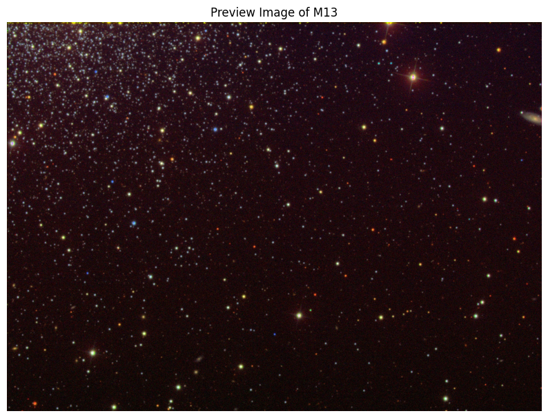
While the field isn’t directly capturing the center of cluster, it will contain enough cluster stars to create a CMD with! We’ll now download the full FITS files and select photoObj-003226-5-0126.fits due to its CMD congruency.
Each photoObj FITS file follows the following naming scheme: photoObj-{RUN}-{CAMCOL}-{FIELD} where RUN is the zero-padded, six-digit identification number for that photometric run, CAMCOL is the camera column identifying the scanline within the run, and FIELD is field number for that observation. The photoObj file contains the fully calibrated FITS files from the SDSS Imaging Pipeline and other respective measurements such as photometry in all five SDSS filters (u, g, r, i, and z), source classification, and quality flags. There is one photoObj file for each run-camcol-field combination.
# Masking the data to extract only the full FITS file
new_products = Observations.filter_products(
    products,
    # Specify FITS files only
    productGroupDescription="Minimum Recommended Products",
    # Select photoObj files (ugriz)
    productSubGroupDescription="SDSS Imaging Catalogs",
    # Select photoObj-003226-5-0126.fits
    productFilename="photoObj-003226-5-0126.fits",
)

# Downloading photoObj-003226-5-0126.fits
manifest = Observations.download_products(new_products, verbose=False)
INFO: Found cached file ./mastDownload/SDSS/sdss_image_003226-5-0126/photoObj-003226-5-0126.fits with expected size 8089920. [astroquery.query]
We can now open the file and examine it. For this tutorial, we will focus on the g-band and r-band magnitudes provided in the first file extension.
The various file extensions are broken down on the SDSS website:
HDU 0: The primary header information.
HDU 1: The photoObj table. This contains information such as magnitudes, coordinates, and flux.
# Opening file
star_array = fits.open(manifest["Local Path"][0])

# Display header info
star_array.info()
Filename: ./mastDownload/SDSS/sdss_image_003226-5-0126/photoObj-003226-5-0126.fits
No.    Name      Ver    Type      Cards   Dimensions   Format
  0  PRIMARY       1 PrimaryHDU      39   ()
  1                1 BinTableHDU    302   2677R x 139C   [19A, 19A, 19A, B, B, B, I, 3A, B, I, I, I, I, J, E, J, J, E, E, E, E, E, E, E, E, 5E, 5E, 5E, 5E, 5E, 5E, 5E, 5E, 5E, 5E, 5E, 5E, 5E, 5E, 5E, 5E, 5E, 5E, 5E, 5E, 5E, 5E, 5E, 5E, 5E, 5E, 5E, 5E, 5E, 5E, 5E, 5E, 5E, 5E, 5E, 5J, 5J, 5J, 5E, 5J, 75E, 75E, 5E, 5E, 5E, 5J, 5E, D, D, D, D, D, D, D, D, D, 5E, 5E, 5E, J, 5E, 5E, 5E, 5E, 5E, 5E, 5E, 5E, 5E, 5E, 5E, 5E, 5E, 5E, 5E, 5E, 5E, 5E, 5E, 5E, 5E, 5E, 5E, 5E, 5E, 5E, 5E, 5E, 5E, 5E, 5E, 5E, 5E, 5E, 5E, 5E, 5E, 5E, 5E, 40E, 40E, 5J, 5J, 5E, 5E, 5D, J, J, J, J, J, J, J, E]
Creating a Color-Magnitude Diagram of M13#
To obtain magnitudes from the FITS file, we’ll be using PSFMAG from the first file extension. Within PSFMAG there are 5 total columns, each one corresponding to the apparent magnitudes in the u, g, r, i, or z filters. We’ll extract the g-band magnitudes from the second column and the r-band magnitudes from the third column.
# Sending the PSFMAG data to a numpy array
magnitudes = star_array[1].data["PSFMAG"]
magnitudes = np.array(magnitudes)

# Creating arrays for g-band and r-band magnitudes
g_band = magnitudes[:, 1]
r_band = magnitudes[:, 2]

# Calculating color (g - r)
color_data1 = g_band - r_band
To create a CMD, we simply need to plot the r-band magnitudes against the color (g-r) for these stars!
# Plotting the CMD
plt.figure(figsize=(8, 6))
plt.scatter(color_data1, r_band, s=3, color="black", label="M13 data")
plt.ylim(10, 30)
plt.gca().invert_yaxis()
plt.xlim(-2, 2)
plt.title("CMD of M13")
plt.ylabel("Apparent Magnitude (r-band)")
plt.xlabel("Color (g - r)")
plt.legend()
plt.grid(True)
plt.tight_layout()
plt.show()
Finding the Distance to M13 Using Data from Gaia#
Gaia was launched by the European Space Agency (ESA) in December 2013. Orbiting at L2, its main purpose is to observe billions of stars to create a 3D map of our galaxy. Gaia provides data such as astrometry, photometry, and radial velocities For more information about Gaia, visit the ESA website.
We’ll query Gaia for M13 data using a search radius of 0.375 degrees. This narrows our search so that we focus on the cluster stars rather than foreground stars, allowing us to get a more accurate distance.
The catalog search should take around a minute or so.
# querying Gaia
coordinates = "16h41m41.24s 36d27m35.5s"  # Coordinates of M13
catalog_data = Catalogs.query_region(
    coordinates, catalog="GaiaDR3", radius=0.375
)
WARNING: InputWarning: Coordinate string is being interpreted as an ICRS coordinate. [astroquery.utils.commons]
Gaia provides parallax measurements for a wide variety of astronomical objects. Stellar parallax is the apparent shift in position of a nearby star caused by Earth’s motion around the Sun.
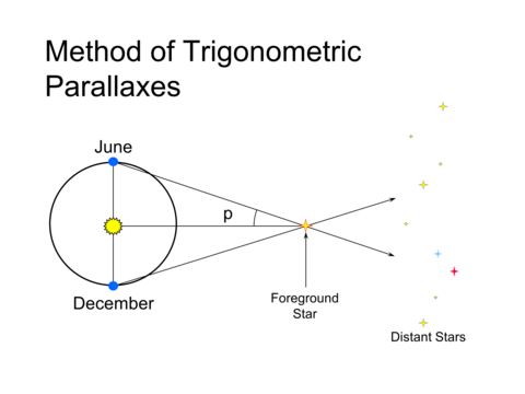
We can determine the distance to these objects from the parallax angle using small-angle approximation:
where \(d\) is distance in parsecs and \(p\) is parallax in arcseconds.
# Extracting parallax measurements from Gaia
parallax = catalog_data["parallax"]  # in milliarcseconds
distance_array = 1 / parallax  # distance array from parallax (kiloparsecs)
ra = catalog_data["ra"]  # right ascension
dec = catalog_data["dec"]  # declination

# Sorting data
sorted_indices = np.argsort(distance_array)
ra_sorted = ra[sorted_indices]
dec_sorted = dec[sorted_indices]
distance_sorted = distance_array[sorted_indices]

# Creating a histogram of the parallax measurements and RA/DEC map
fig, ax = plt.subplots(nrows=1, ncols=2, figsize=(15, 6))

# Histogram
ax[0].hist(parallax, bins=100, color="gray")
ax[0].axvline(
    np.nanmedian(parallax),
    color="red",
    label=f"Median Parallax \n {np.nanmedian(parallax):.3f} milliarcsec",
)
ax[0].set_xlim(-5, 5)
ax[0].set_xticks(np.arange(-5, 5, 1))
ax[0].set_xlabel("Parallax (milliarcseconds)")
ax[0].set_ylabel("Frequency")
ax[0].set_title("Histogram of M13 Parallax Measurements from Gaia")
ax[0].legend()

# RA/DEC map
plot = ax[1].scatter(
    ra_sorted,
    dec_sorted,
    s=2,
    c=distance_sorted,
    cmap="viridis",
    vmin=0,
    vmax=8,
)
cbar = fig.colorbar(plot, ax=ax[1])
cbar.set_label("Distance (kpc)")
ax[1].set_xlabel("RA (degrees)")
ax[1].set_ylabel("DEC (degrees)")
ax[1].set_title("Position of Parallax Measurements Colored by Distance")

plt.show()
/home/runner/micromamba/envs/ci-env/lib/python3.11/site-packages/numpy/lib/_function_base_impl.py:4049: UserWarning: Warning: 'partition' will ignore the 'mask' of the MaskedColumn.
  part.partition(kth)
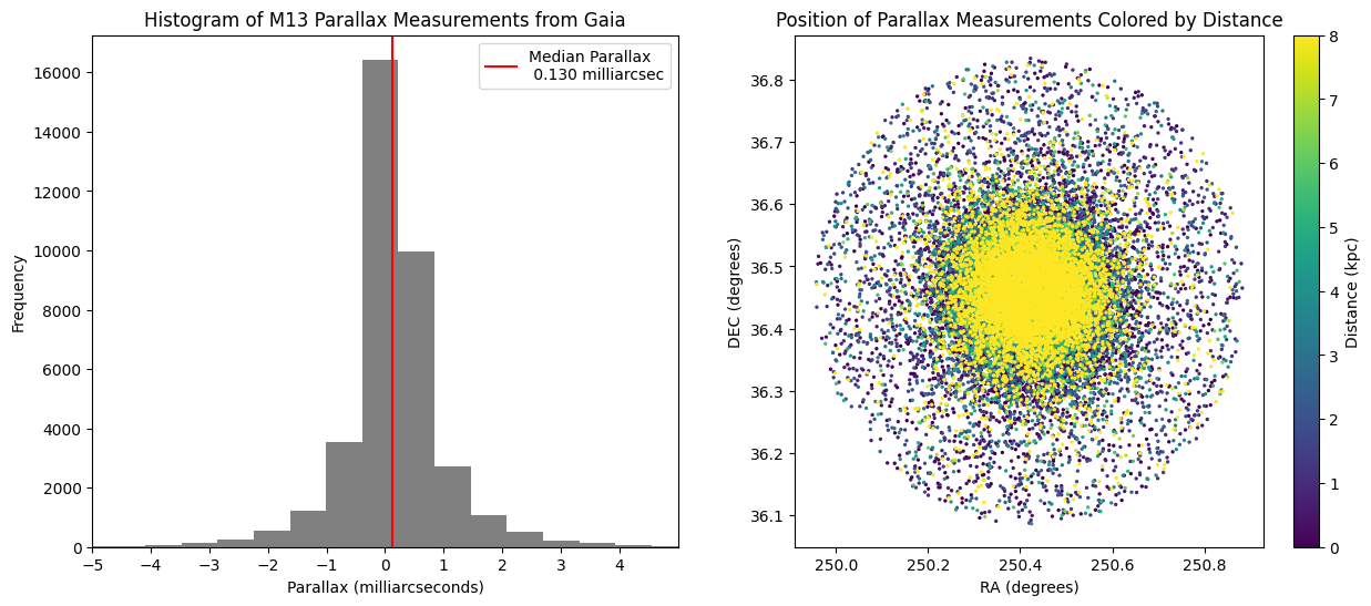
The histogram above shows the distribution of the various parallax measurements Gaia made for M13. We’ll take the median of these measurements to use as a general distance for the cluster.
# Finding the median parallax of the data
cluster_median = np.nanmedian(parallax)

# Calculating distance using stellar parallax formula
distance = 1.0 / cluster_median

print(f"Median Parallax: {cluster_median} milliarcseconds")
print(f"Distance to M13: {distance:.4f} kpc")
Median Parallax: 0.1299530647655502 milliarcseconds
Distance to M13: 7.6951 kpc
Therefore, according to Gaia data, the distance to M13 is approximately 7.6951 kpc. We can now use this to convert the isochrones to apparent magnitudes in the next steps.
Determining the Age of M13 Using Stellar Isochrone Matching#
We can determine the approximate age of M13 by plotting its CMD with isochrones of varying ages, and match the best fit isochrone track to the M13 data.
The isochrones are located in the .txt file isochrones.txt. These were the result of generating isochrones from the PARSEC database with a metallicity of -1.33 dex and ages from 2 billion years old to 14 billion years old in step sizes of 1 billion years. The other settings were left as default.
Since the SDSS Legacy Survey observed apparent magnitudes, we’ll need to convert the absolute magnitudes from the isochrones to apparent magnitudes. We’ll use the distance modulus formula since we know the approximate distance to M13 [9]:
where \(m\) is apparent magnitude, \(M\) is absolute magnitude, and \(d\) is the distance to the object in parsecs.
# Distance to M13
d = distance * 10**3  # parsecs


# Converting absolute magnitudes from isochrones to apparent
def app_mag(M):
    return M + 5 * np.log10(d / 10)
# Importing isochrone .txt file
parsec_data = pd.read_csv(
    "isochrones.txt", sep=r"\s+", comment="#", header=None
)

# Converting the data file to an array
parsec_data = np.array(parsec_data)
# The isochrone data file is broken up into age bins
log_age = [
    9.30103,
    9.47712,
    9.60206,
    9.69897,
    9.77815,
    9.84510,
    9.90309,
    9.95424,
    10.00000,
    10.04139,
    10.07918,
    10.11394,
    10.14613,
]

# Setting up a dictionary
age_data = {}

# Looping through .txt file to separate by age
for i, age in enumerate(log_age, start=1):
    age_data[f"age{i}"] = parsec_data[parsec_data[:, 2] == age]

# Extracting g and r magnitudes, applying distance modulus formula
# Setting up arrays
r_data = []
g_data = []
color_data2 = []

# Sending g and r magnitudes and color to an array
for i in range(1, len(log_age) + 1):
    data = age_data[f"age{i}"]
    g_mag = app_mag(data[:, 29])
    r_mag = app_mag(data[:, 30])
    color = g_mag - r_mag

    r_data.append(r_mag)
    g_data.append(g_mag)
    color_data2.append(color)

# Plotting the isochrones
color = [
    "brown",
    "pink",
    "magenta",
    "purple",
    "navy",
    "darkturquoise",
    "teal",
    "olive",
    "green",
    "gold",
    "orange",
    "lightcoral",
    "red",
]
fig, ax = plt.subplots(figsize=(10, 8))
for i, j, k, r in zip(color_data2, r_data, log_age, color):
    ax.plot(
        i,
        j,
        alpha=0.5,
        label=f"{(10**k) / 1e9:.0f} billion years old",
        color=r,
    )

# Plotting the data
ax.scatter(
    color_data1,
    r_band,
    marker="x",
    linewidth=0.9,
    s=20,
    color="black",
    label="SDSS data of M13",
)
ax.set_ylabel("Apparent Magnitude (r-band)")
ax.set_xlabel("Color (g - r)")
ax.set_title("Color - Magnitude Diagram of M13 with Isochrones")
ax.set_ylim(10, 30)
ax.set_xlim(-2, 2)
ax.invert_yaxis()
ax.legend(fontsize=10)
ax.grid(True)
fig.tight_layout()
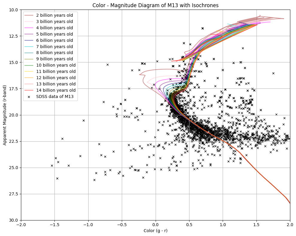
While the isochrones extend beyond 27.5 r-band magnitude, the M13 data doesn’t quite reach this far due to the limiting magnitude of the SDSS camera.
We’ll create a zoomed-in plot to further study the terminal age main sequence (TAMS) and main sequence turnoff phases.
# Replotting with different x and y limits
ax.set_xlim(0, 0.9)
ax.set_ylim(16, 20)
ax.invert_yaxis()
ax.legend(fontsize=8)

# Adding annotation for main sequence turnoff
circle = plt.Circle(
    (0.35, 17.75),
    0.25,
    color="red",
    fill=False,
    linewidth=2,
    label="Main Sequence Turnoff",
)
ax.add_patch(circle)
ax.annotate(
    "Main Sequence Turnoff",
    xy=(0.6, 17.75),
    xytext=(0.6 + 0.05, 17.75 - 0.2),
    arrowprops=dict(arrowstyle="->", color="red"),
    fontsize=12,
    color="red",
)

fig
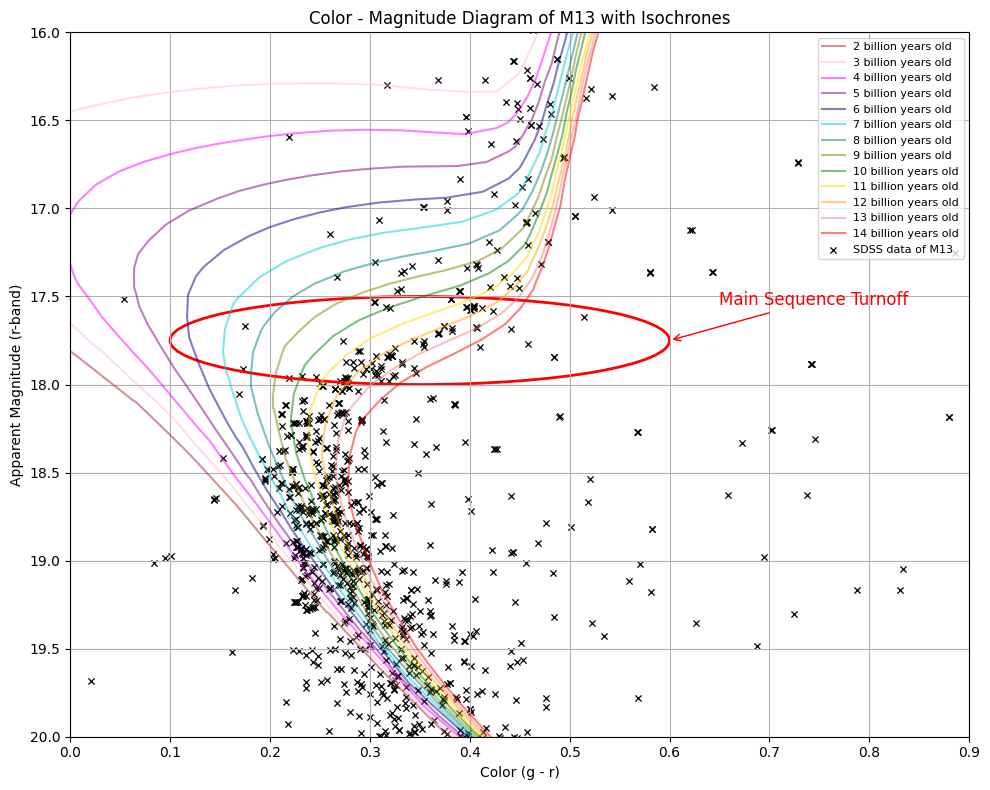
From examining the data and isochrones within the main sequence turnoff circle, it appears the data follow the orange track, indicating the cluster is approximately 12 billion years old. This isn’t far from the 11.65 billion year old estimate made by D. Forbes and T. Bridges in Accreted Versus in situ Milky Way Globular Clusters [5].
End of Tutorial#
Congratulations, you now know how to determine the age of a star cluster from isochrone matching using the SDSS Legacy Imaging Survey!
Exercises#
Now it’s your turn to determine the age of Messier 3! M3 has a metallicity of -1.34 dex, which is nearly identical to M13, so you can use the same isochrone file isochrones.txt [5].
There are six different fields available for M3, you can choose whichever one visually has the best looking CMD when plotted, so answers can vary slightly.
# Query SDSS Legacy Imaging Survey for M3 data
# View available products
# Download products
# Plot CMD of M3
# Find distance to M3 using Gaia
# Plot CMD with isochrones
Exercise Solutions#
# Query SDSS Legacy Imaging Survey for M3 data

obs_table2 = Observations.query_criteria(
    objectname="M3", provenance_name="SDSS Legacy Imaging"
)

# Displaying the table
obs_table2
| intentType | obs_collection | provenance_name | instrument_name | project | filters | wavelength_region | target_name | target_classification | obs_id | s_ra | s_dec | dataproduct_type | proposal_pi | calib_level | t_min | t_max | t_exptime | em_min | em_max | obs_title | t_obs_release | proposal_id | proposal_type | sequence_number | s_region | jpegURL | dataURL | dataRights | mtFlag | srcDen | obsid | objID | objID1 | distance |
|---|---|---|---|---|---|---|---|---|---|---|---|---|---|---|---|---|---|---|---|---|---|---|---|---|---|---|---|---|---|---|---|---|---|---|
| str7 | str4 | str19 | str11 | str4 | str9 | str7 | str13 | str5 | str24 | float64 | float64 | str5 | str18 | int64 | float64 | float64 | float64 | float64 | float64 | str51 | float64 | str3 | str1 | int64 | str197 | str61 | str61 | str6 | bool | float64 | str9 | str9 | str9 | float64 |
| science | SDSS | SDSS Legacy Imaging | SDSS Camera | SDSS | u;g;r;i;z | OPTICAL | 004649-3-0147 | FIELD | sdss_image_004649-3-0147 | 205.657671944 | 28.0589023561 | image | SDSS Collaboration | 3 | 53148.29295949074 | 53148.29690089648 | 53.907456 | 304.79999999999995 | 1083.3000000000002 | Sloan Digital Sky Survey (SDSS) Legacy Imaging Data | 55571.0 | N/A | -- | -- | POLYGON 205.54394470283248 27.962474450750673 205.5888145108555 28.184009933873277 205.77158117037538 28.15512819922499 205.72634720424867 27.933652309716898 205.54394470283248 27.962474450750673 | mast:SDSS/sdss/imaging/4649/3/147/frame-irg-004649-3-0147.jpg | mast:SDSS/sdss/imaging/4649/3/147/photoObj-004649-3-0147.fits | PUBLIC | False | nan | 297003774 | 876981454 | 876981454 | 707.4595416072544 |
| science | SDSS | SDSS Legacy Imaging | SDSS Camera | SDSS | u;g;r;i;z | OPTICAL | 004649-3-0146 | FIELD | sdss_image_004649-3-0146 | 205.490651819 | 28.085188819 | image | SDSS Collaboration | 3 | 53148.292544791664 | 53148.29648631315 | 53.907456 | 304.79999999999995 | 1083.3000000000002 | Sloan Digital Sky Survey (SDSS) Legacy Imaging Data | 55571.0 | N/A | -- | -- | POLYGON 205.37706850623056 27.988627871719682 205.42159486278487 28.210231791472925 205.60441753406982 28.181547849750537 205.5595262109013 27.960003124274728 205.37706850623056 27.988627871719682 | mast:SDSS/sdss/imaging/4649/3/146/frame-irg-004649-3-0146.jpg | mast:SDSS/sdss/imaging/4649/3/146/photoObj-004649-3-0146.fits | PUBLIC | False | nan | 297016644 | 877000851 | 877000851 | 662.4582359914772 |
| science | SDSS | SDSS Legacy Imaging | SDSS Camera | SDSS | u;g;r;i;z | OPTICAL | 004649-3-0145 | FIELD | sdss_image_004649-3-0145 | 205.323553735 | 28.1112790851 | image | SDSS Collaboration | 3 | 53148.29213043981 | 53148.296071498335 | 53.907456 | 304.79999999999995 | 1083.3000000000002 | Sloan Digital Sky Survey (SDSS) Legacy Imaging Data | 55571.0 | N/A | -- | -- | POLYGON 205.2100784323227 28.01456697081828 205.25425945894472 28.23622770285823 205.43721195883117 28.207789375478082 205.392665007371 27.986187458585785 205.2100784323227 28.01456697081828 | mast:SDSS/sdss/imaging/4649/3/145/frame-irg-004649-3-0145.jpg | mast:SDSS/sdss/imaging/4649/3/145/photoObj-004649-3-0145.fits | PUBLIC | False | nan | 297021749 | 877008987 | 877008987 | 704.6808153444647 |
| science | SDSS | SDSS Legacy Imaging | SDSS Camera | SDSS | u;g;r;i;z | OPTICAL | 004649-4-0147 | FIELD | sdss_image_004649-4-0147 | 205.741895083 | 28.47212241 | image | SDSS Collaboration | 3 | 53148.292959375 | 53148.29690078074 | 53.907456 | 304.79999999999995 | 1083.3000000000002 | Sloan Digital Sky Survey (SDSS) Legacy Imaging Data | 55571.0 | N/A | -- | -- | POLYGON 205.62768552230045 28.37577168647357 205.67284676286525 28.597293482580454 205.85629075716403 28.568269370809166 205.81075776098697 28.346808356990465 205.62768552230045 28.37577168647357 | mast:SDSS/sdss/imaging/4649/4/147/frame-irg-004649-4-0147.jpg | mast:SDSS/sdss/imaging/4649/4/147/photoObj-004649-4-0147.fits | PUBLIC | False | nan | 297041189 | 877038782 | 877038782 | 251.12717566712155 |
| science | SDSS | SDSS Legacy Imaging | SDSS Camera | SDSS | u;g;r;i;z | OPTICAL | 004649-4-0146 | FIELD | sdss_image_004649-4-0146 | 205.574278356 | 28.4985213252 | image | SDSS Collaboration | 3 | 53148.292544791664 | 53148.29648619741 | 53.907456 | 304.79999999999995 | 1083.3000000000002 | Sloan Digital Sky Survey (SDSS) Legacy Imaging Data | 55571.0 | N/A | -- | -- | POLYGON 205.4602440816663 28.401990585237147 205.50501052174238 28.623614315047135 205.68849923575618 28.594848487893643 205.64336014259345 28.37328506246469 205.4602440816663 28.401990585237147 | mast:SDSS/sdss/imaging/4649/4/146/frame-irg-004649-4-0146.jpg | mast:SDSS/sdss/imaging/4649/4/146/photoObj-004649-4-0146.fits | PUBLIC | False | nan | 297055298 | 877061020 | 877061020 | 38.70436560786968 |
| science | SDSS | SDSS Legacy Imaging | SDSS Camera | SDSS | u;g;r;i;z | OPTICAL | 004649-4-0145 | FIELD | sdss_image_004649-4-0145 | 205.406518204 | 28.5247113578 | image | SDSS Collaboration | 3 | 53148.29212997685 | 53148.296071382596 | 53.907456 | 304.79999999999995 | 1083.3000000000002 | Sloan Digital Sky Survey (SDSS) Legacy Imaging Data | 55571.0 | N/A | -- | -- | POLYGON 205.29256303409997 28.428055614125235 205.33703079237077 28.649688467782617 205.52066047872054 28.621163594869746 205.47581916619885 28.399590727008345 205.29256303409997 28.428055614125235 | mast:SDSS/sdss/imaging/4649/4/145/frame-irg-004649-4-0145.jpg | mast:SDSS/sdss/imaging/4649/4/145/photoObj-004649-4-0145.fits | PUBLIC | False | nan | 297060525 | 877069703 | 877069703 | 243.55720045892613 |
| science | SDSS | SDSS Legacy Imaging | SDSS Camera | SDSS | u;g;r;i;z | OPTICAL | 004646-3-0082 | FIELD | sdss_image_004646-3-0082 | 205.656308884 | 28.2721588412 | image | SDSS Collaboration | 3 | 53147.302064814816 | 53147.306005641854 | 53.907456 | 304.79999999999995 | 1083.3000000000002 | Sloan Digital Sky Survey (SDSS) Legacy Imaging Data | 55571.0 | N/A | -- | -- | POLYGON 205.5423832905099 28.175729968111437 205.58730682675895 28.39725991057679 205.77041863016308 28.368384857511558 205.7251269725764 28.146914991664634 205.5423832905099 28.175729968111437 | mast:SDSS/sdss/imaging/4646/3/82/frame-irg-004646-3-0082.jpg | mast:SDSS/sdss/imaging/4646/3/82/photoObj-004646-3-0082.fits | PUBLIC | False | nan | 298416340 | 886143838 | 886143838 | 108.59459460943275 |
| science | SDSS | SDSS Legacy Imaging | SDSS Camera | SDSS | u;g;r;i;z | OPTICAL | 004646-3-0081 | FIELD | sdss_image_004646-3-0081 | 205.488943252 | 28.2984535321 | image | SDSS Collaboration | 3 | 53147.30165 | 53147.305590595555 | 53.907456 | 304.79999999999995 | 1083.3000000000002 | Sloan Digital Sky Survey (SDSS) Legacy Imaging Data | 55571.0 | N/A | -- | -- | POLYGON 205.3751517797895 28.20190784674507 205.41974839794054 28.423509196402975 205.60291927098706 28.394796490690652 205.55795372445033 28.173254838069173 205.3751517797895 28.20190784674507 | mast:SDSS/sdss/imaging/4646/3/81/frame-irg-004646-3-0081.jpg | mast:SDSS/sdss/imaging/4646/3/81/photoObj-004646-3-0081.fits | PUBLIC | False | nan | 298416749 | 886147617 | 886147617 | 0.0 |
| science | SDSS | SDSS Legacy Imaging | SDSS Camera | SDSS | u;g;r;i;z | OPTICAL | 004646-3-0080 | FIELD | sdss_image_004646-3-0080 | 205.321501743 | 28.3245630156 | image | SDSS Collaboration | 3 | 53147.301235416664 | 53147.305176127964 | 53.907456 | 304.79999999999995 | 1083.3000000000002 | Sloan Digital Sky Survey (SDSS) Legacy Imaging Data | 55571.0 | N/A | -- | -- | POLYGON 205.20778823297513 28.22786559996562 205.2520733711031 28.449521548371912 205.43540036111 28.421057749901465 205.39074528505412 28.1994611700242 205.20778823297513 28.22786559996562 | mast:SDSS/sdss/imaging/4646/3/80/frame-irg-004646-3-0080.jpg | mast:SDSS/sdss/imaging/4646/3/80/photoObj-004646-3-0080.fits | PUBLIC | False | nan | 298418227 | 886162128 | 886162128 | 379.99380206335434 |
| science | SDSS | SDSS Legacy Imaging | SDSS Camera | SDSS | u;g;r;i;z | OPTICAL | 004646-3-0083 | FIELD | sdss_image_004646-3-0083 | 205.823590943 | 28.2456434759 | image | SDSS Collaboration | 3 | 53147.302479398146 | 53147.306420225184 | 53.907456 | 304.79999999999995 | 1083.3000000000002 | Sloan Digital Sky Survey (SDSS) Legacy Imaging Data | 55571.0 | N/A | -- | -- | POLYGON 205.7095285185484 28.149375294418277 205.75479948691986 28.370854782021958 205.93783702450116 28.341708656515983 205.89219879256294 28.120289646216374 205.7095285185484 28.149375294418277 | mast:SDSS/sdss/imaging/4646/3/83/frame-irg-004646-3-0083.jpg | mast:SDSS/sdss/imaging/4646/3/83/photoObj-004646-3-0083.fits | PUBLIC | False | nan | 298419600 | 886176841 | 886176841 | 647.5256341960012 |
# Download products
products2 = Observations.get_product_list(obs_table2)

# Download products
new_products2 = Observations.filter_products(
    products2,
    # Specify FITS files only
    productGroupDescription="Minimum Recommended Products",
    # Select photoObj files (ugriz)
    productSubGroupDescription="SDSS Imaging Catalogs",
    # Select photoObj-003226-5-0126.fits
    productFilename="photoObj-004649-4-0145.fits",
)

# Downloading photoObj-003226-5-0126.fits
manifest2 = Observations.download_products(new_products2)
INFO: Found cached file ./mastDownload/SDSS/sdss_image_004649-4-0145/photoObj-004649-4-0145.fits with expected size 7848000. [astroquery.query]
# Plot CMD of M3
# Opening file
star_array2 = fits.open(manifest2["Local Path"][0])
# Sending the PSFMAG data to a numpy array
magnitudes2 = star_array2[1].data["PSFMAG"]
magnitudes2 = np.array(magnitudes2)
# Creating arrays for g-band and r-band magnitudes
g_band2 = magnitudes2[:, 1]
r_band2 = magnitudes2[:, 2]
# Calculating color (g - r)
color_data3 = g_band2 - r_band2
# Plotting the CMD
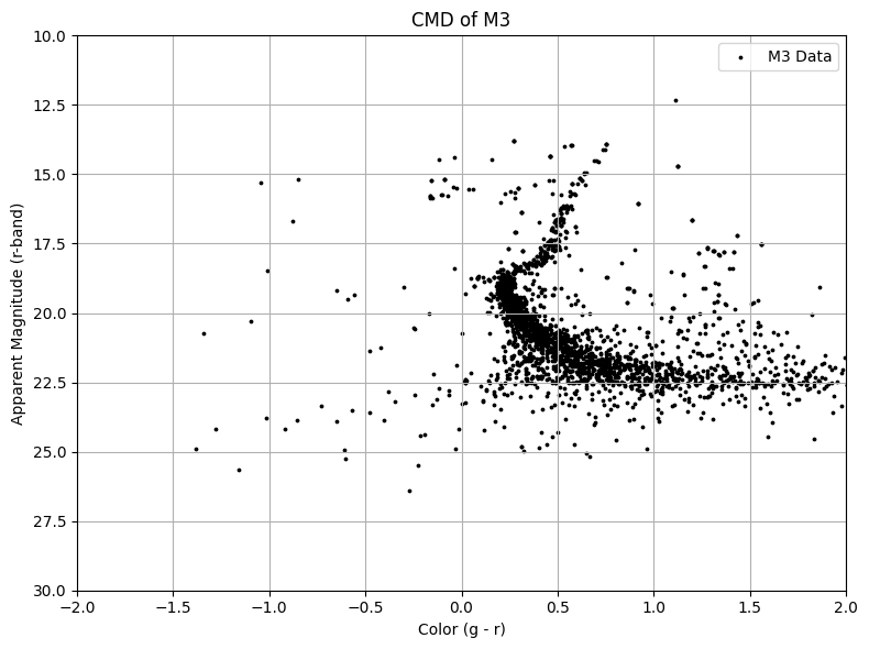
plt.figure(figsize=(8, 6))
plt.scatter(color_data3, r_band2, s=3, color="black", label="M3 Data")
plt.ylim(10, 30)
plt.gca().invert_yaxis()
plt.xlim(-2, 2)
plt.title("CMD of M3")
plt.ylabel("Apparent Magnitude (r-band)")
plt.xlabel("Color (g - r)")
plt.legend()
plt.grid(True)
plt.tight_layout()
plt.show()
# Find distance to M3 using Gaia

# querying Gaia
coordinates2 = "13h42m11.80s 28d22m31.69s"  # Coordinates of M3

catalog_data2 = Catalogs.query_region(
    coordinates2, catalog="GaiaDR3", radius=0.35
)

# Extracting parallax measurements from Gaia
parallax2 = catalog_data2["parallax"]  # in milliarcseconds
distance_array2 = 1 / parallax2  # distance array from parallax (kiloparsecs)
ra2 = catalog_data2["ra"]  # right ascension
dec2 = catalog_data2["dec"]  # declination

# Sorting data
sorted_indices2 = np.argsort(distance_array2)
ra_sorted2 = ra2[sorted_indices2]
dec_sorted2 = dec2[sorted_indices2]
distance_sorted2 = distance_array2[sorted_indices2]

# Creating a histogram of the parallax measurements and RA/DEC map
fig2, ax2 = plt.subplots(nrows=1, ncols=2, figsize=(15, 6))

# Histogram
ax2[0].hist(parallax2, bins=100, color="gray")
ax2[0].axvline(
    np.nanmedian(parallax2),
    color="red",
    label=f"Median Parallax \n {np.nanmedian(parallax2):.3f} milliarcsec",
)
ax2[0].set_xlim(-5, 5)
ax2[0].set_xticks(np.arange(-5, 5, 1))
ax2[0].set_xlabel("Parallax (milliarcseconds)")
ax2[0].set_ylabel("Frequency")
ax2[0].set_title("Histogram of M3 Parallax Measurements from Gaia")
ax2[0].legend()

# RA/DEC map
plot2 = ax2[1].scatter(
    ra_sorted2,
    dec_sorted2,
    s=2,
    c=distance_sorted2,
    cmap="viridis",
    vmin=0,
    vmax=8,
)
cbar2 = fig.colorbar(plot2, ax=ax2[1])
cbar2.set_label("Distance (kpc)")
ax2[1].set_xlabel("RA (degrees)")
ax2[1].set_ylabel("DEC (degrees)")
ax2[1].set_title("Position of Parallax Measurements Colored by Distance")

plt.show()

# Finding the median parallax of the data
cluster_median2 = np.nanmedian(parallax2)

# Calculating distance using stellar parallax formula
distance2 = 1.0 / cluster_median2

print(f"Median Parallax: {cluster_median2} milliarcseconds")
print(f"Distance to M3: {distance2:.4f} kpc")

# Distance to M3
d2 = distance2 * 10**3  # parsecs
WARNING: InputWarning: Coordinate string is being interpreted as an ICRS coordinate. [astroquery.utils.commons]
/home/runner/micromamba/envs/ci-env/lib/python3.11/site-packages/numpy/lib/_function_base_impl.py:4049: UserWarning: Warning: 'partition' will ignore the 'mask' of the MaskedColumn.
  part.partition(kth)
/tmp/ipykernel_2822/104144980.py:49: UserWarning: Adding colorbar to a different Figure <Figure size 1500x600 with 3 Axes> than <Figure size 1000x800 with 1 Axes> which fig.colorbar is called on.
  cbar2 = fig.colorbar(plot2, ax=ax2[1])

Median Parallax: 0.09967599714927582 milliarcseconds
Distance to M3: 10.0325 kpc
# Plot CMD with isochrones


def app_mag2(M):
    return M + 5 * np.log10(d2 / 10)


r_data2 = []
g_data2 = []
color_data4 = []

for i in range(1, len(log_age) + 1):
    data = age_data[f"age{i}"]
    g_mag = app_mag2(data[:, 29])
    r_mag = app_mag2(data[:, 30])
    color2 = g_mag - r_mag

    r_data2.append(r_mag)
    g_data2.append(g_mag)
    color_data4.append(color2)

fig, ax = plt.subplots(figsize=(10, 8))
for i, j, k, r in zip(color_data4, r_data2, log_age, color):
    ax.plot(
        i,
        j,
        alpha=0.5,
        label=f"{(10**k) / 1e9:.0f} billion years old",
        color=r,
    )

# Plotting the data
ax.scatter(
    color_data3,
    r_band2,
    marker="x",
    linewidth=0.9,
    s=20,
    color="black",
    label="SDSS data of M3",
)
ax.set_ylabel("Apparent Magnitude (r-band)")
ax.set_xlabel("Color (g - r)")
ax.set_title("Color - Magnitude Diagram of M3 with Isochrones")
ax.set_ylim(10, 30)
ax.set_xlim(-2, 2)
ax.invert_yaxis()
ax.legend(fontsize=10)
ax.grid(True)
fig.tight_layout()
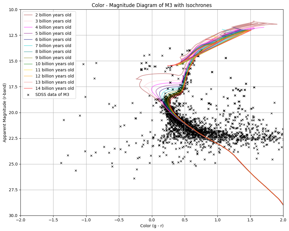
# Replotting with different x and y limits
ax.set_xlim(0, 0.9)
ax.set_ylim(16, 20)
ax.invert_yaxis()
ax.legend(fontsize=8)

# Adding annotation for main sequence turnoff
circle = plt.Circle(
    (0.35, 18.25),
    0.25,
    color="red",
    fill=False,
    linewidth=2,
    label="Main Sequence Turnoff",
)
ax.add_patch(circle)
ax.annotate(
    "Main Sequence Turnoff",
    xy=(0.6, 18.25),
    xytext=(0.6 + 0.05, 17.75 - 0.2),
    arrowprops=dict(arrowstyle="->", color="red"),
    fontsize=12,
    color="red",
)

fig
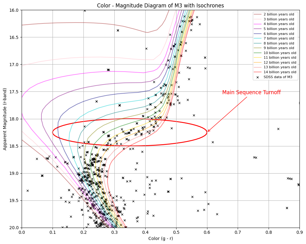
Results: The data for M3 appear to fit between the yellow and orange lines. Therefore, M3 is between 11-12 billion years old!
This matches the age estimates of approximately 8-11.4 billion years.
Addtional Resources#
Additional resources are linked below:
Citations#
If you use data from MAST for published research, please see the following links for information on which citations to include in your paper:
About this Notebook#
Author(s): Natalie Haugen (nhaugen@terpmail.umd.edu) and Julie Imig (jimig@stsci.edu)
Keyword(s): Tutorial, SDSS, SDSS Legacy Imaging Survey, stars, HR diagram, CMD, imaging
First published: July 2025
Last updated: July 2025