ACS/WFC Image Reduction

ACS/WFC Image Reduction#

Introduction#

This notebook covers the steps necessary to calibrate Advanced Camera for Surveys (ACS) Wide Field Channel (WFC) observations to produce a distortion-corrected image ready for photometry.

For most observations, reprocessing the raw files with the calibration pipeline is no longer required as the MAST archive is now static and any changes to the pipeline or reference files automatically triggers a reprocessing of the data. However, users may wish to reprocess their data with custom reference files.

This notebook is intended for users with a (very!) basic understanding of python and photometry.

You will need approximately 13 GB of space available for this exercise.

This tutorial will show you how to…#

1. Calibrate Raw Files#

Query the Calibration Reference Data System (CRDS) for the current best reference files applicable to a given observation
Update the *_raw.fits primary headers with new calibration information
Retrieve calibration files from CRDS and set up the reference file directory
Process files with calacs

2. Update the WCS#

Update the FLT/FLC file WCS header keywords

Imports#

Here we list the Python packages used in this notebook. Links to the documentation for each module is provided for convenience.

Package Name	module	docs	used for
`os`	`system`	link	command line input
`os`	`environ`	link	setting environments
`shutil`	`rmtree`	link	remove directory tree
`glob`	`glob`	link	search for files based on Unix shell rules
`astroquery.mast`	`Observations`	link	download data from MAST
`astropy.io`	`fits`	link	access and update fits files
`astropy.table`	`Table`	link	constructing and editing in a tabular format
`stwcs`	`updatewcs`	link	update wcs solution

import os
import shutil
import glob

from astroquery.mast import Observations

from astropy.io import fits

from stwcs import updatewcs

from p_module import plot

Download the Data #

Here we download all of the data required for this notebook. This is an important step! Some of the image processing steps require all relevant files to be in the working directory. We recommend working with a brand new directory for every new set of data.

GO Proposal 10775: “An ACS Survey of Galactic Globular Clusters”#

For this example, we will only retreive data associated with the Observation ID J9L960010. Using the python package astroquery, we can access the MAST archive.

We will need to grab the raw files, the telemetry files, and the association file for this observation set.

MAY CHANGE: The argument "mrp_only" stands for "minimum recommended products only". It currently needs to be set to False, although in the future, False is intended to be set as the default and can be left out.

obs_table = Observations.query_criteria(proposal_id=10775, obs_id='J9L960010')


dl_table = Observations.download_products(obs_table['obsid'],
                                          productSubGroupDescription=['RAW', 'ASN', 'SPT'],
                                          mrp_only=False)

We’ll use the packages os and shutil to put all of these files in our working directory and do a little housekeeping.

for row in dl_table:
    oldfname = row['Local Path']
    newfname = os.path.basename(oldfname)
    os.rename(oldfname, newfname)
    
# Delete the mastDownload directory and all subdirectories it contains.
shutil.rmtree('mastDownload')

Here we set our filenames to variable names for convenience using glob.glob.

asn_file = 'j9l960010_asn.fits'
raw_files = glob.glob('*_raw.fits')

File Information#

The structure of the fits files from ACS may be different depending on what kind of observation was made. For more information, refer to Section 2.2 of the ACS Data Handbook.

Association Files#

Ext	Name	Type	Contains
0	PRIMARY	(PrimaryHDU)	Meta-data related to the entire file.
1	ASN (Association)	(BinTableHDU)	Table of files associated with this group.

Raw Files (WFC-Specific)#

Ext	Name	Type	Contains
0	PRIMARY	(PrimaryHDU)	Meta-data related to the entire file.
1	SCI (Image)	(ImageHDU)	WFC2 raw image data.
2	ERR (Error)	(ImageHDU)	WFC2 error array.
3	DQ (Data Quality)	(ImageHDU)	WFC2 data quality array.
4	SCI (Image)	(ImageHDU)	WFC1 raw image data.
5	ERR (Error)	(ImageHDU)	WFC1 error array.
6	DQ (Data Quality)	(ImageHDU)	WFC1 data quality array.

You can always use .info() on an HDUlist for an overview of the structure

with fits.open(asn_file) as hdulist:
    hdulist.info()
    
with fits.open(raw_files[0]) as hdulist:
    hdulist.info()

Calibrate Raw Files #

Now that we have the *_raw.fits files, we can process them with the ACS calibration pipeline calacs.

Updating Headers for CRDS#

By default, the association file will trigger the creation of a drizzled product. In order to avoid this, we will filter the association file to only include table entries with MEMTYPE equal to ‘EXP-DTH’. This will remove the ‘PROD-DTH’ entry that prompts AstroDrizzle.

with fits.open(asn_file, mode='update') as asn_hdu:
    asn_tab = asn_hdu[1].data
    asn_tab = asn_tab[asn_tab['MEMTYPE'] == 'EXP-DTH']

Due to the computationally intense processing required to CTE correct full-frame ACS/WFC images, we have disabled the CTE correction here by default, however it can be turned on by changing the following variable to True:

cte_correct = False

Calibration steps can be enabled or disabled by setting the switch keywords in the primary header to ‘PERFORM’ or ‘OMIT’, respectively. Switch keywords all end with the string CORR (e.g., BLEVCORR and DARKCORR). In this case, we want to update PCTECORR.

for file in raw_files:
    
    if cte_correct: 
        value = 'PERFORM'
    else: 
        value = 'OMIT'
        
    fits.setval(file, 'PCTECORR', value=value)

Querying CRDS for Reference Files#

Before running calacs, we need to set some environment variables for several subsequent calibration tasks.

We will point to a subdirectory called crds_cache/ using the JREF environment variable. The JREF variable is used for ACS reference files. Other instruments use other variables, e.g., IREF for WFC3.

os.environ['CRDS_SERVER_URL'] = 'https://hst-crds.stsci.edu'
os.environ['CRDS_SERVER'] = 'https://hst-crds.stsci.edu'
os.environ['CRDS_PATH'] = './crds_cache'
os.environ['jref'] = './crds_cache/references/hst/acs/'

The code block below will query CRDS for the best reference files currently available for these datasets, update the header keywords to point “to these new files. We will use the Python package os to run terminal commands. In the terminal, the line would be:

crds bestrefs --files [filename] --sync-references=1 --update-bestrefs

…where ‘filename’ is the name of your fits file.

for file in raw_files:
    command_line_input = 'crds bestrefs --files {:} --sync-references=1 --update-bestrefs'.format(file)
    os.system(command_line_input)

Running calacs#

Finally, we can run calacs on the association file. It will produce *_flt.fits. The FLT files have had the default CCD calibration steps (bias subtraction, dark subtraction, flat field normalization) performed.

If the CTE correction is enabled...

…this next step will take a long time to complete. The CTE correction is computationally expensive and will use all of the cores on a machine by default. On an 8 core machine, CTE correcting a full-frame ACS/WFC image can take approximately 15 minutes per RAW file.
…*_flc.fits will also be produced. The FLC files are CTE-corrected but otherwise identical to the FLT files.

os.system('calacs.e j9l960010_asn.fits')

Selecting an image to plot, depending on whether or not you enabled CTE correction earlier.

if cte_correct:
    fl_fits = 'j9l960a7q_flc.fits'
else:
    fl_fits = 'j9l960a7q_flt.fits'

Plotting results#

As a check of our calibrated products, we will plot a subsection of one of the input images.

raw_image = fits.getdata('j9l960a7q_raw.fits')
cal_image = fits.getdata(fl_fits)

plot.calib_compare_plot(raw_image, cal_image)

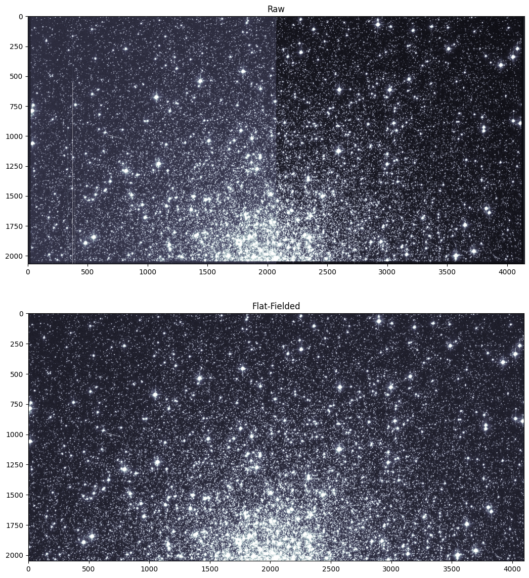
Comparing the FLT calibrated image to the RAW uncalibrated one, we can see that image artifacts have been removed. Most noticeably, hot columns in the bias have been subtracted.

if cte_correct:
    img_files = 'j9l9*a[9-f]q_flc.fits'
else:
    img_files = 'j9l9*a[9-f]q_flt.fits'

updatewcs.updatewcs(img_files, use_db=False)

Conclusion#

The FLT and FLC images are not yet suitable for photometry. Before performing any analysis on the images, we still need to remove detector artifacts, cosmic rays, and geometric distortion. AstroDrizzle can do all of these steps and produce a single mosaic image that incorporates all of the individual exposures.

Users who do not use astrodrizzle to correct data for distortion will need to apply a pixel area map to their data to correct for the distorted pixel area projected onto the sky before performing photometry. For those who would like to learn how to create a pixel area map, a Jupyter Notebook on the subject can be found here.

For more help:#

More details may be found on the ACS website and in the ACS Instrument and Data Handbooks.

Please visit the HST Help Desk. Through the help desk portal, you can explore the HST Knowledge Base and request additional help from experts.

Top of Page