
Correcting for Scattered Light in WFC3/IR Exposures: Manually Subtracting Bad Reads#
Learning Goals#
This notebook presents one of two available methods to correct for a time variable background (TVB) due to scattered light from observing close to the Earth’s limb. This method illustrates how to manually subtract any bad reads from the final exposure read of the WFC3/IR IMA data.
By the end of this tutorial, you will:
Compute and plot the difference between IMA reads to identify those affected by TVB.
Correct a single exposure in which the first few reads are affected by scattered light by subtracting those “bad” reads from the final IMA read.
Compare the original FLT to the reprocessed FLT image.
Compare the original DRZ to the reprocessed DRZ image.
A second method for correcting TVB (masking bad reads in the RAW image and re-running calwf3) can be found in the notebook Correcting for Scattered Light in WFC3/IR Exposures: Using calwf3 to Mask Bad Reads (O’Connor 2023). This method performs the ‘ramp
fitting’ step in calwf3 and therefore removes cosmic rays from the final image. It only works,
however, when TVB occurs at the beginning or end of the IR exposure and may leave sky
residuals in regions flagged as IR ‘blobs’.
Please note that the FLT products in this notebook are really ‘corrected IMA’
files and therefore do not include the ‘ramp fitting’ step in calwf3. The final images will
therefore still contain cosmic rays, and these artifacts may be removed using software such
as AstroDrizzle when combining multiple exposures.
Table of Contents#
Introduction
1. Imports
2. Downloading Data
3. Identifying Reads with Earth-limb Scattered Light
4. Querying CRDS for the Reference File
6. Drizzling Nominal and Reprocessed FLT Products
7. Conclusions
Additional Resources
About this Notebook
Citations
Introduction #
WFC3 images can be affected by many different kinds of unwanted, non-science features, such as satellite trails, peculiar cosmic rays, Earth-limb scattered light, reflections off the filter wheel, and more. We call these features “anomalies”. The majority of these anomalies are well studied, correctable, and easily identifiable, as discussed in WFC3 ISR 2017-22.
In this notebook, we will walk through the process of correcting WFC3/IR images for anomalies that appear in only some of the reads (see section 7.7 of the WFC3 Instrument Handboook for a discussion of the WFC3/IR MULTIACCUM observing mode). We examine an observation affected by a strong TVB due to Earth limb scattered light affecting the first few reads (section 7.10 of the WFC3 Data Handbook). We will manually subtract the affected reads from the final read of the IMA and copy the updated science and error arrays into the FLT science and error arrays. This method is based on section 5 of WFC3 ISR 2016-16: ‘Excising Individual Reads’. This same method can be used to remove individual reads that contain other anomalies, such as satellite trails.
This new FLT will have a reduced total exposure time (and signal-to-noise) given the rejection of some number of reads but will now have a flat background and an improved ramp fit.
Please see the notebook WFC3/IR IMA Visualization with An Example of Time Variable Background (O’Connor 2023) for a walkthrough of how to identify a TVB due to scattered light.
1. Imports #
This notebook assumes you have created the virtual environment in WFC3 Library’s installation instructions.
We import:
os for setting environment variables
shutil for managing directories
numpy for handling array functions
matplotlib.pyplot for plotting data
astropy.io fits for accessing FITS files
astroquery.mast Observations for downloading data
wfc3tools
calwf3for calibrating WFC3 dataginga for finding min/max outlier pixels
stwcs for updating World Coordinate System images
drizzlepac for combining images with AstroDrizzle
We import the following modules:
ima_visualization_and_differencing to take the difference between reads, plot the ramp, and visualize the difference in images
import os
import shutil
import numpy as np
from matplotlib import pyplot as plt
from astropy.io import fits
from astroquery.mast import Observations
from wfc3tools import calwf3
from ginga.util.zscale import zscale
from stwcs import updatewcs
from drizzlepac import astrodrizzle

import ima_visualization_and_differencing as diff

%matplotlib inline
2. Downloading Data#
The following commands query MAST for the necessary data products and download them to the current directory. Here we obtain WFC3/IR observations from HST Frontier Fields program 14037, Visit BB. We specifically want the observation “icqtbbbxq”, as it is strongly affected by Earth limb scattered light. The data products requested are the RAW, IMA, and FLT files.
Warning: this cell may take a few minutes to complete.
OBS_ID = 'ICQTBB020'
data_list = Observations.query_criteria(obs_id=OBS_ID)

file_id = "icqtbbbxq"
Observations.download_products(data_list['obsid'],
                               project='CALWF3',
                               obs_id=file_id,
                               cache=False,
                               mrp_only=False,
                               productSubGroupDescription=['RAW', 'IMA', 'FLT'])
Downloading URL https://mast.stsci.edu/api/v0.1/Download/file?uri=mast:HST/product/icqtbbbxq_ima.fits to ./mastDownload/HST/icqtbbbxq/icqtbbbxq_ima.fits ...
[Done]
Downloading URL https://mast.stsci.edu/api/v0.1/Download/file?uri=mast:HST/product/icqtbbbxq_flt.fits to ./mastDownload/HST/icqtbbbxq/icqtbbbxq_flt.fits ...
[Done]
Downloading URL https://mast.stsci.edu/api/v0.1/Download/file?uri=mast:HST/product/icqtbbbxq_raw.fits to ./mastDownload/HST/icqtbbbxq/icqtbbbxq_raw.fits ...
[Done]
| Local Path | Status | Message | URL |
|---|---|---|---|
| str47 | str8 | object | object |
| ./mastDownload/HST/icqtbbbxq/icqtbbbxq_ima.fits | COMPLETE | None | None |
| ./mastDownload/HST/icqtbbbxq/icqtbbbxq_flt.fits | COMPLETE | None | None |
| ./mastDownload/HST/icqtbbbxq/icqtbbbxq_raw.fits | COMPLETE | None | None |
Now, we will copy our RAW file into our working directory to use in this tutorial. We copy the IMA and FLT files to a new directory called “orig/” for later use.
if not os.path.exists('orig/'):
    os.mkdir('orig/')

shutil.copy(f'mastDownload/HST/{file_id}/{file_id}_ima.fits', f'orig/{file_id}_ima.fits')
shutil.copy(f'mastDownload/HST/{file_id}/{file_id}_flt.fits', f'orig/{file_id}_flt.fits')

raw_file = f'mastDownload/HST/{file_id}/{file_id}_raw.fits'

shutil.copy(raw_file, f'{file_id}_raw.fits')
'icqtbbbxq_raw.fits'
3. Identifying Reads with Earth-limb Scattered Light#
In this section, we show how to identify the reads impacted by the scattered light by examining the difference in count rate between reads. This section was taken from the WFC3/IR IMA Visualization with An Example of Time Variable Background (O’Connor 2023) notebook, which includes a more comprehensive walkthrough of identifying time variable background.
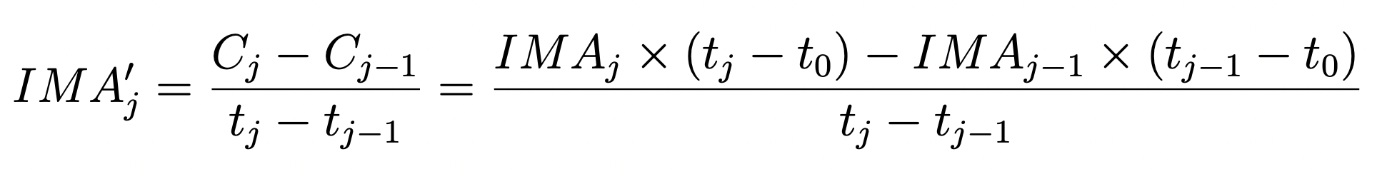
Here we implement a technique to examine the count rate difference between consecutive reads. In this case, we first convert from count rate (electrons/second) back to counts (electrons) before taking the difference, as shown in equation 3 from WFC3 ISR 2018-05.
We compare sky values in different regions of the detector (left side, right side, and full frame). If you would like to specify your own regions for the left and right sides of your image, you can change the lhs_region and rhs_region parameters. Each region must be specified as a dictionary including the four “corners” (x0, x1, y0, and y1) of the region you would like to select. You may want to avoid the edges of the detector which have a large number of bad pixels and higher flat field errors.
fig = plt.figure(figsize=(20, 10))

ima_filepath = f'orig/{file_id}_ima.fits'

path, filename = os.path.split(ima_filepath)
cube, integ_time = diff.read_wfc3(ima_filepath)


lhs_region = {"x0": 50, "x1": 250, "y0": 100, "y1": 900}
rhs_region = {"x0": 700, "x1": 900, "y0": 100, "y1": 900}

# Please use a limit that makes sense for your own data, when running your images through this notebook.
cube[np.abs(cube) > 3] = np.nan

diff_cube = diff.compute_diff_imas(cube, integ_time, diff_method="instantaneous")
median_diff_fullframe, median_diff_lhs, median_diff_rhs = (
    diff.get_median_fullframe_lhs_rhs(diff_cube,
                                      lhs_region=lhs_region,
                                      rhs_region=rhs_region))
plt.rc('xtick', labelsize=20)
plt.rc('ytick', labelsize=20)
plt.rcParams.update({'font.size': 30})
plt.rcParams.update({'lines.markersize': 15})

diff.plot_ramp(ima_filepath, integ_time, median_diff_fullframe,
               median_diff_lhs, median_diff_rhs)

plt.ylim(0.5, 2.5)
_ = plt.title(filename)
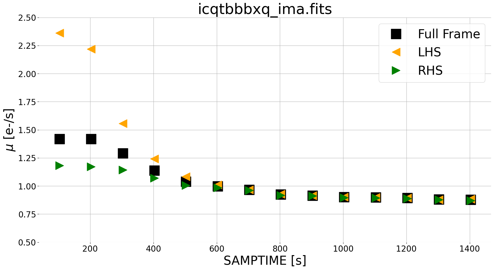
Here, we utilize a few functions from our module ima_visualization_and_differencing. We use read_wfc3 to grab the IMA data from all reads and corresponding integration times. We also implement upper and lower limits on our pixel values to exclude sources when plotting our ramp. We take the instantaneous difference using compute_diff_imas, which computes the difference as described in the equation above. Finally, we use plot_ramp to plot the median count rate from the left side, right side, and full frame image.
For our scattered light exposure, we see zodiacal light at a level of ~0.9e/s in later reads, with the scattered light component affecting the first several reads where the median count rate for the left side (orange triangles) is larger than the right side (green triangles). We can visualize this in 2 dimensions in the panel plot below, using plot_ima_difference_subplots.
In the panel plot, we see that sources (small galaxies) are visible in the difference images using this new method. Note that this may complicate the analysis of the spatial background (e.g. left versus right) for images with extended targets, such as large galaxies. In this case, users may wish to adjust the regions of the detector used for the ramp plots. We therefore recommend inspecting both the panel plots as well as the ramp fits for diagnosing any issues with the data.
fig = plt.figure(figsize=(20, 10))

ima_filepath = f'orig/{file_id}_ima.fits'

lhs_region = {"x0": 50, "x1": 250, "y0": 100, "y1": 900}
rhs_region = {"x0": 700, "x1": 900, "y0": 100, "y1": 900}

diff.plot_ima_difference_subplots(ima_filepath,
                                  difference_method='instantaneous',
                                  lhs_region=lhs_region,
                                  rhs_region=rhs_region)
<Figure size 2000x1000 with 0 Axes>
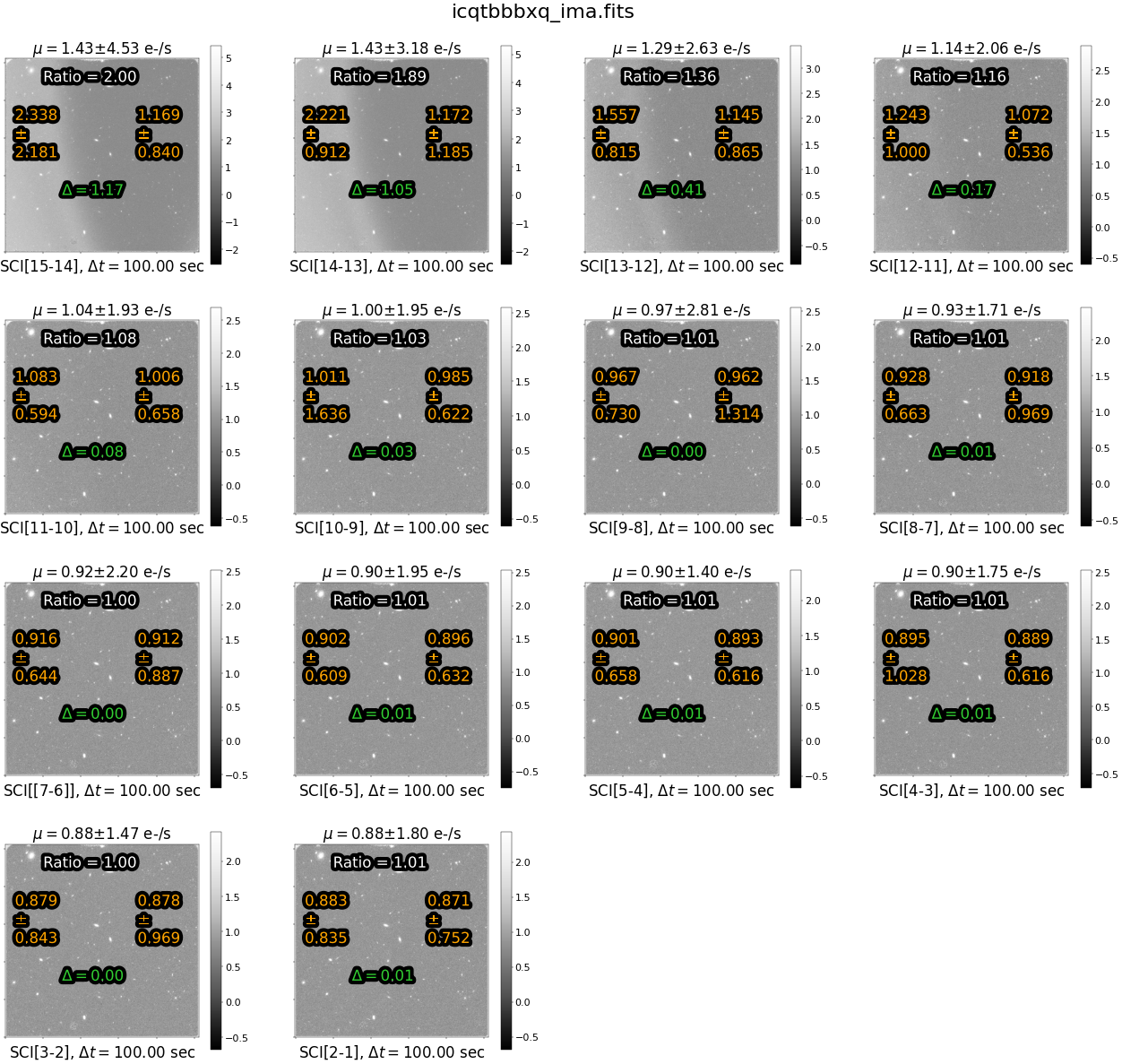
In this figure, we see that the ratio of instantaneous rate for the left versus right side of the image is ~1.0 for all but the first few reads (which are affected by scattered light). We choose to exclude reads with a ratio greater than 1.1 from the final science data, as they are the reads most strongly affected by scattered light. While this reduces the total exposure from 1403 to 1000 seconds, it removes the spatial component from the sky background.
4. Querying CRDS for the Reference File#
In this notebook, we will run calwf3 to produce an IMA file, which we will use to remove bad reads. Before running calwf3, we need to set some environment variables.
We will point to a subdirectory called crds_cache using the IREF environment variable, which is used for WFC3 reference files. Other instruments use other variables, e.g., JREF for ACS.
os.environ['CRDS_SERVER_URL'] = 'https://hst-crds.stsci.edu'
os.environ['CRDS_SERVER'] = 'https://hst-crds.stsci.edu'
os.environ['CRDS_PATH'] = './crds_cache'
os.environ['iref'] = './crds_cache/references/hst/wfc3/'
The code block below will query CRDS for the best reference files currently available for our dataset and update the header keywords to point to these new files. We will use os to run terminal commands. In the terminal, the line would be:
…where ‘filename’ is the name of your fits file.
Warning: this cell may take a few minutes to complete.
raw_filepath = f'{file_id}_raw.fits'

print(f"Querying CRDS for the reference file associated with {raw_filepath}.")
command_line_input = 'crds bestrefs --files {:} --sync-references=1 --update-bestrefs'.format(raw_filepath)
os.system(command_line_input)
Querying CRDS for the reference file associated with icqtbbbxq_raw.fits.
CRDS - INFO - No comparison context or source comparison requested.
CRDS - INFO - ===> Processing icqtbbbxq_raw.fits
CRDS - INFO -  0 errors
CRDS - INFO -  0 warnings
CRDS - INFO -  2 infos
0
5. Correcting the Data#
To address anomalies such as scattered light, satellite trails, and more in WFC3/IR images we can remove the individual affected reads and correct the science and error arrays accordingly. For our example image, we choose to exclude reads where the ratio of background signal is greater than 1.1 e-/s (see the notebook WFC3/IR IMA Visualization with An Example of Time Variable Background (O’Connor 2023) for a more complete demonstration of how we find this ratio).
5.1 Excising “Bad” Reads #
In this section, we walk through the key steps to removing bad reads.
We select our excluded reads (in this case reads reads SCI,15 through SCI, 11) and use the “remove_reads” function to effectively subtract out the reads affected by TVB.
The key steps to this process are:
Run
calwf3on the RAW image file to produce an IMA and an FLT.Take the IMA file and subtract the science array from the “bad” reads from the cumulative exposure.
Correct the final integration time accordingly.
Correct the error image extension to reflect the changes to the science array.
Update the final FLT headers, science array, and error array.
We walk through this process below.
STEP 1: Run calwf3#
bad_reads = [11, 12, 13, 14, 15] # note, we leave the "zero read" (read number 16)

# Remove any existing ima or flt products from working directory or calwf3 will not run
for ext in ['flt', 'ima']:
    if os.path.exists(raw_filepath.replace('raw', ext)):
        os.remove(raw_filepath.replace('raw', ext))
# run CALWF3
calwf3(raw_filepath)
git tag: 0090c701-dirty

git branch: HEAD

HEAD @: 0090c701d894003cfc690e9f8d5fde81e6939090


CALBEG*** CALWF3 -- Version 3.7.2 (Apr-15-2024) ***

Begin    02-Dec-2025 20:17:42 UTC


Input    icqtbbbxq_raw.fits

loading asn


LoadAsn:  Processing SINGLE exposure

Trying to open icqtbbbxq_raw.fits...

Read in Primary header from icqtbbbxq_raw.fits...

Revising existing trailer file `icqtbbbxq.tra'.


CALBEG*** WF3IR -- Version 3.7.2 (Apr-15-2024) ***

Begin    02-Dec-2025 20:17:42 UTC

Input    icqtbbbxq_raw.fits

Output   icqtbbbxq_flt.fits

Trying to open icqtbbbxq_raw.fits...

Read in Primary header from icqtbbbxq_raw.fits...

APERTURE IR-FIX

FILTER   F140W

DETECTOR IR

Reading data from icqtbbbxq_raw.fits ...

CCDTAB   iref$t2c16200i_ccd.fits

CCDTAB   PEDIGREE=Ground

CCDTAB   DESCRIP =Reference data based on Thermal-Vac #3, gain=2.5 results for IR-4

CCDTAB   DESCRIP =Readnoise,gain,saturation from TV3,MEB2 values. ISRs 2008-25,39,50

    readnoise =20.2,19.8,19.9,20.1

    gain =2.34,2.37,2.31,2.38

DQICORR  PERFORM

DQITAB   iref$3562014hi_bpx.fits

DQITAB   PEDIGREE=INFLIGHT 03/11/2015 12/09/2016

DQITAB   DESCRIP =Bad Pixel Table generated using Cycle 23 Flats and Darks-----------

DQICORR  COMPLETE

ZSIGCORR PERFORM
ZSIGCORR detected 1286 saturated pixels in 0th read

ZSIGCORR detected 1346 saturated pixels in 1st read

ZSIGCORR COMPLETE

BLEVCORR PERFORM

OSCNTAB  iref$q911321mi_osc.fits

OSCNTAB  PEDIGREE=GROUND

OSCNTAB  DESCRIP =Initial values for ground test data processing

BLEVCORR COMPLETE

ZOFFCORR PERFORM

ZOFFCORR COMPLETE

NOISCORR PERFORM

Uncertainty array initialized.

NOISCORR COMPLETE

NLINCORR PERFORM

NLINFILE iref$9au15283i_lin.fits

NLINFILE PEDIGREE=INFLIGHT 29/03/2011 25/11/2012

NLINFILE DESCRIP =Non-linearity, pixel-based correction from WFC3 on-orbit frames

NLINCORR detected 1286 saturated pixels in imset 16
NLINCORR detected 1349 saturated pixels in imset 15

NLINCORR detected 1461 saturated pixels in imset 14

NLINCORR detected 1515 saturated pixels in imset 13

NLINCORR detected 1569 saturated pixels in imset 12
NLINCORR detected 1623 saturated pixels in imset 11

NLINCORR detected 1689 saturated pixels in imset 10

NLINCORR detected 1742 saturated pixels in imset 9

NLINCORR detected 1798 saturated pixels in imset 8
NLINCORR detected 1844 saturated pixels in imset 7

NLINCORR detected 1894 saturated pixels in imset 6

NLINCORR detected 1952 saturated pixels in imset 5

NLINCORR detected 2011 saturated pixels in imset 4
NLINCORR detected 2087 saturated pixels in imset 3

NLINCORR detected 2166 saturated pixels in imset 2

NLINCORR detected 2244 saturated pixels in imset 1

NLINCORR COMPLETE

DARKCORR PERFORM

DARKFILE iref$35620125i_drk.fits

DARKFILE PEDIGREE=INFLIGHT 04/09/2009 14/11/2016

DARKFILE DESCRIP =Dark Created from 142 frames spanning cycles 17 to 24--------------

DARKCORR using dark imset 16 for imset 16 with exptime=       0

DARKCORR using dark imset 15 for imset 15 with exptime= 2.93229
DARKCORR using dark imset 14 for imset 14 with exptime= 102.933

DARKCORR using dark imset 13 for imset 13 with exptime= 202.933
DARKCORR using dark imset 12 for imset 12 with exptime= 302.933

DARKCORR using dark imset 11 for imset 11 with exptime= 402.934
DARKCORR using dark imset 10 for imset 10 with exptime= 502.934

DARKCORR using dark imset  9 for imset  9 with exptime= 602.934
DARKCORR using dark imset  8 for imset  8 with exptime= 702.934

DARKCORR using dark imset  7 for imset  7 with exptime= 802.935
DARKCORR using dark imset  6 for imset  6 with exptime= 902.935

DARKCORR using dark imset  5 for imset  5 with exptime= 1002.94
DARKCORR using dark imset  4 for imset  4 with exptime= 1102.94

DARKCORR using dark imset  3 for imset  3 with exptime= 1202.94
DARKCORR using dark imset  2 for imset  2 with exptime= 1302.94

DARKCORR using dark imset  1 for imset  1 with exptime= 1402.94
DARKCORR COMPLETE

PHOTCORR PERFORM

IMPHTTAB iref$8ch15233i_imp.fits

IMPHTTAB PEDIGREE=INFLIGHT 08/05/2009 01/09/2024

IMPHTTAB DESCRIP =Time-dependent image photometry reference table (IMPHTTAB)---------

Found parameterized variable 1.

NUMPAR=1, N=1

Allocated 1 parnames

Adding parameter mjd#57339.3673 as parnames[0]

==> Value of PHOTFLAM = 1.4769486e-20

==> Value of PHOTPLAM = 13922.907

==> Value of PHOTBW = 1132.39

PHOTCORR COMPLETE

UNITCORR PERFORM

UNITCORR COMPLETE

CRCORR   PERFORM

CRREJTAB iref$u6a1748ri_crr.fits

CRIDCALC using 4 sigma rejection threshold

               256 bad DQ mask

               4 max CRs for UNSTABLE
65 pixels detected as unstable

CRCORR   COMPLETE

FLATCORR PERFORM

PFLTFILE iref$4ac19224i_pfl.fits

PFLTFILE PEDIGREE=INFLIGHT 31/07/2009 05/12/2019

PFLTFILE DESCRIP =Sky Flat from Combined In-flight observations between 2009 and 2019

DFLTFILE iref$4ac18162i_dfl.fits

DFLTFILE PEDIGREE=INFLIGHT 31/07/2009 05/12/2019

DFLTFILE DESCRIP =Delta-Flat for IR Blobs by Date of Appearance from Sky Flat Dataset

FLATCORR COMPLETE

Writing calibrated readouts to icqtbbbxq_ima.fits
Writing final image to icqtbbbxq_flt.fits

 with trimx = 5,5, trimy = 5,5


End      02-Dec-2025 20:17:47 UTC

*** WF3IR complete ***


End      02-Dec-2025 20:17:47 UTC

*** CALWF3 complete ***

CALWF3 completion for icqtbbbxq_raw.fits
STEP 2: Correct the IMA product#
Here we walk through the process of subtracting the reads affected by Earth-limb scattered light from the cumulative science extension of the IMA. While an FLT product is also created in step 1, we do not use this file due to the poor-quality ramp fit in the presence of TVB.
Overall, the steps are as follows:
Load the science data as a 3D array and the integration time as a 1D array from the science and time extensions of the IMA file. In addition, load the associated dark reference file.
ima_filepath_new = f'{file_id}_ima.fits'
with fits.open(ima_filepath_new) as ima:
    cube, integ_time = diff.read_wfc3(ima_filepath_new)
    dark_file = ima[0].header['DARKFILE'].replace('iref$', os.getenv('iref'))
    dark_counts, dark_time = diff.read_wfc3(dark_file)
Convert science data from electrons/second to electrons.
cube_counts = np.zeros(np.shape(cube))

for img in range(cube.shape[2]):
    cube_counts[:, :, img] = cube[:, :, img]*integ_time[img]
Compute the difference between reads (the cumulative difference, in this case) to isolate counts and integration time from bad reads.
cube_diff = np.diff(cube_counts, axis=2)
dark_diff = np.diff(dark_counts, axis=2)
dt = np.diff(integ_time)
For each bad read, subtract the counts (and time) from ONLY that read from the total data.
final_dark = dark_counts[:, :, -1]

final_sci = cube_counts[:, :, -1]
final_time = np.ones((1024, 1024))*integ_time[-1]

if (len(bad_reads) > 0):
    for read in bad_reads:
        index = cube_counts.shape[2]-read-1
        final_sci -= cube_diff[:, :, index]
        final_dark -= dark_diff[:, :, index]
        final_time -= dt[index]
STEP 3: Correct the Error Image#
The errors associated with the raw data are estimated according to the noise model for the detector which currently includes a simple combination of detector readnoise and poisson noise from the pixel and which is intended to replicate the calwf3 error array calculation. Currently, the inital detector noise model (in electrons) is as follows, where RN is the readnoise.
Note that our signal equation includes flat and dark corrections to revert the final science array (flux) produced by calwf3 to the original signal (in electrons) recorded in the detector.
The ERR array continues to be updated as the SCI array is processed. The dark error term is added in quadrature as the dark current is subtracted from the science array:
Next, the flat images are divided out of the science image. There are two flat-fields (p-flat and delta-flat), which are each divided out of the science image. The flat errors are combined using the correct error propagation method.
P-Flat (pflat) file:
Delta-Flat (dflat) file:
and finally it is converted to an error in electrons/second as:
Evaluating this equation, we come up with an equation for error array calculation (in electrons/second) which we use in our Python calculations as follows:
We do not address the error propagation through the nonlinearity correction step of calwf3 (NLINCORR), as it is complicated and sufficiently small to be outside of the scope of this notebook.
# Readnoise in 4 amps
RN = np.zeros((1024, 1024))
RN[512:, 0:512] += ima[0].header['READNSEA']
RN[0:512, 0:512] += ima[0].header['READNSEB']
RN[0:512, 512:] += ima[0].header['READNSEC']
RN[512:, 512:] += ima[0].header['READNSED']

# Gain in 4 amps
gain_2D = np.zeros((1024, 1024))
gain_2D[512:, 0:512] += ima[0].header['ATODGNA']
gain_2D[0:512, 0:512] += ima[0].header['ATODGNB']
gain_2D[0:512, 512:] += ima[0].header['ATODGNC']
gain_2D[512:, 512:] += ima[0].header['ATODGND']

# Dark image
with fits.open(dark_file) as dark_im:

    # Grabbing the flats
    pflat_file = ima[0].header['PFLTFILE'].replace('iref$', os.getenv('iref'))
    dflat_file = ima[0].header['DFLTFILE'].replace('iref$', os.getenv('iref'))

    with fits.open(pflat_file) as pflat_im, fits.open(dflat_file) as dflat_im:
        pflat = pflat_im[1].data
        dflat = dflat_im[1].data

        # Computing the final error

        # Poisson error: sqrt(signal), flux = final_sci, dark is converted to electrons
        signal = (final_sci*(pflat*dflat)+final_dark*gain_2D)

        # Flat errors
        dflat_err = dflat_im['ERR'].data
        pflat_err = pflat_im['ERR'].data

        # Dark error
        dark_err = (dark_im['ERR'].data)*gain_2D

        # Final error term
        final_err = np.sqrt(RN**2 + signal + (dark_err**2) + (pflat_err*final_sci*dflat)**2
                            + (dflat_err*final_sci*pflat)**2)
        final_err /= (pflat*dflat*final_time)
        final_err[np.isnan(final_err)] = 0

        # Finally the final science image is converted back to count rate
        final_sci /= final_time
STEP 4: Update the FLT Product#
Finally, we update the FLT product created in step 1 with the new science array, error array, and header keywords (such as the new total exposure time).
flt_filepath_new = f'{file_id}_flt.fits'
with fits.open(flt_filepath_new, mode='update') as flt:

    # Updating the flt data
    flt['SCI'].data = final_sci[5:-5, 5:-5]
    flt['ERR'].data = final_err[5:-5, 5:-5]

    # Updating the FLT header
    flt[0].header['IMA2FLT'] = (1, 'FLT extracted from IMA file')
    flt[0].header['EXPTIME'] = np.max(final_time)
    flt[0].header['NPOP'] = (len(bad_reads), 'Number of reads popped from the sequence')
Putting It All Together#
Below, we have included the entire correction process (steps 1-4 above) in a function, for convenience.
def remove_reads(raw_filepath, bad_reads=[]):
    '''
    From the final IMA read, subtract data of reads affected by anomalies.
    Compute a corrected science image and error image, and place them in the FLT product.

    Parameters
    ----------
    raw_filepath: str
        Path to a RAW full-frame IR image fits file.

    bad_reads: list of int
        List of the IMSET numbers (science extension numbers) of reads affected by anomalies.
    '''

    flt_filepath = raw_filepath.replace('raw', 'flt')
    ima_filepath = raw_filepath.replace('raw', 'ima')

    # Remove existing products or calwf3 will die
    for filepath in [flt_filepath, ima_filepath]:
        if os.path.exists(filepath):
            os.remove(filepath)

    # Run calwf3
    calwf3(raw_filepath)

    # Take calwf3 produced IMA, get rid of bad reads
    with fits.open(ima_filepath) as ima:

        cube, integ_time = diff.read_wfc3(ima_filepath)

        dark_file = ima[0].header['DARKFILE'].replace('iref$', os.getenv('iref'))
        dark_counts, dark_time = diff.read_wfc3(dark_file)

        cube_counts = np.zeros(np.shape(cube))
        for img in range(cube.shape[2]):
            cube_counts[:, :, img] = cube[:, :, img]*integ_time[img]

        cube_diff = np.diff(cube_counts, axis=2)
        dark_diff = np.diff(dark_counts, axis=2)
        dt = np.diff(integ_time)

        final_dark = dark_counts[:, :, -1]
        final_sci = cube_counts[:, :, -1]
        final_time = np.ones((1024, 1024))*integ_time[-1]

        if (len(bad_reads) > 0):
            for read in bad_reads:
                index = cube_counts.shape[2]-read-1
                final_sci -= cube_diff[:, :, index]
                final_dark -= dark_diff[:, :, index]
                final_time -= dt[index]

        # Variance terms
        # Readnoise in 4 amps
        RN = np.zeros((1024, 1024))
        RN[512:, 0:512] += ima[0].header['READNSEA']
        RN[0:512, 0:512] += ima[0].header['READNSEB']
        RN[0:512, 512:] += ima[0].header['READNSEC']
        RN[512:, 512:] += ima[0].header['READNSED']

        # Gain in 4 amps
        gain_2D = np.zeros((1024, 1024))
        gain_2D[512:, 0:512] += ima[0].header['ATODGNA']
        gain_2D[0:512, 0:512] += ima[0].header['ATODGNB']
        gain_2D[0:512, 512:] += ima[0].header['ATODGNC']
        gain_2D[512:, 512:] += ima[0].header['ATODGND']

        # Dark image
        with fits.open(dark_file) as dark_im:

            # Grabbing the flats
            pflat_file = ima[0].header['PFLTFILE'].replace('iref$', os.getenv('iref'))
            dflat_file = ima[0].header['DFLTFILE'].replace('iref$', os.getenv('iref'))
            with fits.open(pflat_file) as pflat_im, fits.open(dflat_file) as dflat_im:
                pflat = pflat_im[1].data
                dflat = dflat_im[1].data

                # Computing the final error

                # Poisson error: sqrt(signal), flux = final_sci, dark is converted to electrons
                signal = (final_sci*(pflat*dflat)+final_dark*gain_2D)
                # Flat errors
                dflat_err = dflat_im['ERR'].data
                pflat_err = pflat_im['ERR'].data
                # Dark error
                dark_err = (dark_im['ERR'].data)*gain_2D

                # Final error term
                final_err = np.sqrt(RN**2 + signal + (dark_err**2) + (pflat_err*final_sci*dflat)**2
                                    + (dflat_err*final_sci*pflat)**2)

                final_err /= (pflat*dflat*final_time)
                final_err[np.isnan(final_err)] = 0

                # Finally the final science image (converted back to count rate)
                final_sci /= final_time

                # Updating the flt data
                with fits.open(flt_filepath, mode='update') as flt:

                    flt['SCI'].data = final_sci[5:-5, 5:-5]
                    flt['ERR'].data = final_err[5:-5, 5:-5]

                    # Updating the FLT header
                    flt[0].header['IMA2FLT'] = (1, 'FLT extracted from IMA file')
                    flt[0].header['EXPTIME'] = np.max(final_time)
                    flt[0].header['NPOP'] = (len(bad_reads), 'Number of reads popped from the sequence')
5.2 Comparing FLT Products #
You may want to move your reprocessed images to a new directory, especially if you plan to run the notebook again.
reprocessed_flt = f'{file_id}_flt.fits'

original_flt = f'orig/{file_id}_flt.fits'
Now, we can compare our original and reprocessed FLT products.
with fits.open(reprocessed_flt) as image_new, fits.open(original_flt) as image_old:
    fig = plt.figure(figsize=(20, 7))
    fig
    rows = 1
    columns = 2

    # Add the total exptime in the title
    ax1 = fig.add_subplot(rows, columns, 1)
    ax1.set_title("Reprocessed FLT image", fontsize=20)
    im1 = plt.imshow(image_new["SCI", 1].data, vmin=0.8, vmax=1.3,
                     origin='lower', cmap='Greys_r')
    ax1.tick_params(axis='both', labelsize=10)
    cbar1 = plt.colorbar(im1, ax=ax1)
    cbar1.ax.tick_params(labelsize=10)

    ax2 = fig.add_subplot(rows, columns, 2)
    ax2.set_title("Original FLT image", fontsize=20)
    im2 = plt.imshow(image_old["SCI", 1].data, vmin=0.8, vmax=1.3,
                     origin='lower',  cmap='Greys_r')
    ax2.tick_params(axis='both', labelsize=10)
    cbar2 = plt.colorbar(im2, ax=ax2)
    cbar2.ax.tick_params(labelsize=10)

    plt.rc('xtick', labelsize=10)
    plt.rc('ytick', labelsize=10)
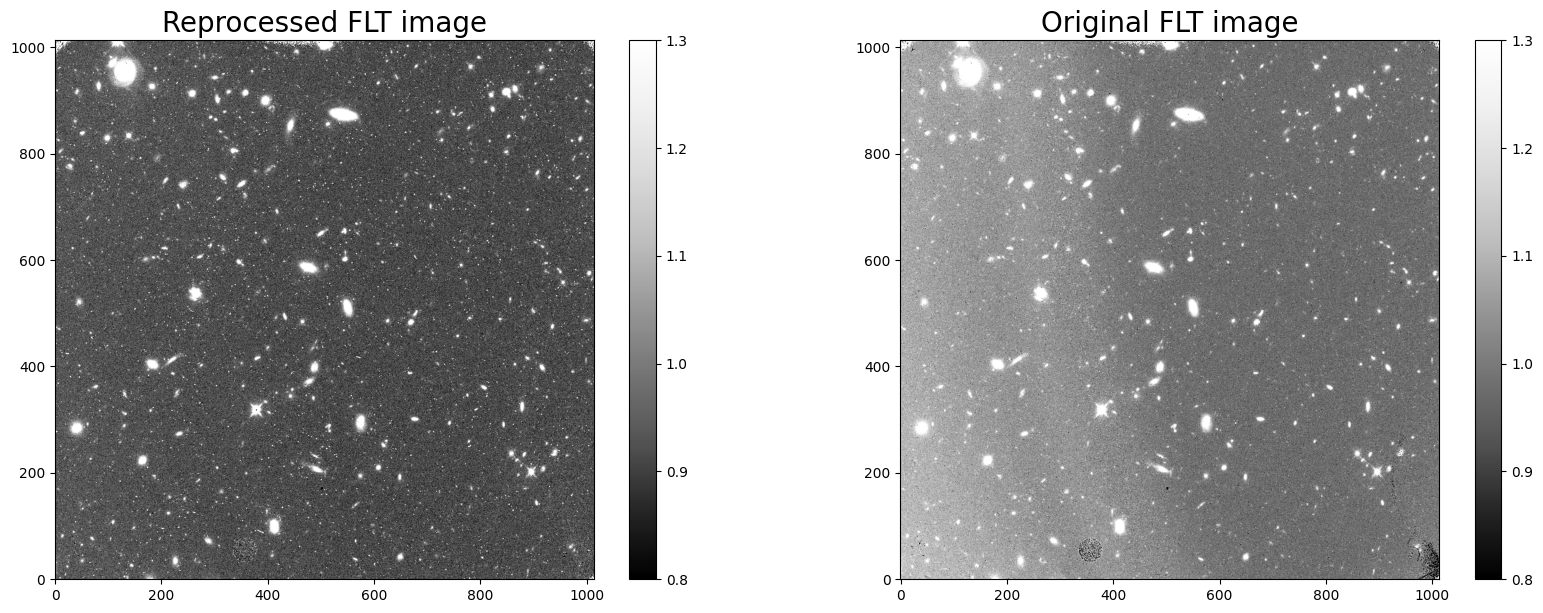
This new image was produced by subtracting the signal from the first 5 reads (not including the 0 read) from the final science data, reducing the effective exposure time from 1403 to 1000 seconds. While the total exposure is reduced from 1403 seconds to 1000 seconds (thus decreasing the overall S/N of the image), the background in the reprocessed image is now uniform over the entire field of view. We can see that the new FLT image is free of the Earth limb scattered light visible in the old FLT image.
print('The final exposure time after reprocessing is {}.'.format(image_new[0].header['EXPTIME']))
The final exposure time after reprocessing is 1000.0032699999998.
6. Drizzling Nominal and Reprocessed FLT Products #
In our example we use an exposure (icqtbbbxq) from image association ICQTBB020 acquired in visit BB of program 14037. This visit consists of two orbits of two exposures each, and we now download the three other FLTs in the visit (icqtbbc0q_flt.fits, icqtbbbrq_flt.fits, icqtbbbtq_flt.fits) and the pipeline drizzled DRZ product.
To produce a clean DRZ image (without cosmic rays), we can drizzle the four FLTs together (from the nominal exposures and the reprocessed exposure).
data_list = Observations.query_criteria(obs_id=OBS_ID)

Observations.download_products(data_list['obsid'], project='CALWF3', cache=False,
                               mrp_only=False, productSubGroupDescription=['FLT', 'DRZ'])
Downloading URL https://mast.stsci.edu/api/v0.1/Download/file?uri=mast:HST/product/icqtbbbrq_flt.fits to ./mastDownload/HST/icqtbbbrq/icqtbbbrq_flt.fits ...
[Done]
Downloading URL https://mast.stsci.edu/api/v0.1/Download/file?uri=mast:HST/product/icqtbbbtq_flt.fits to ./mastDownload/HST/icqtbbbtq/icqtbbbtq_flt.fits ...
[Done]
Downloading URL https://mast.stsci.edu/api/v0.1/Download/file?uri=mast:HST/product/icqtbbbxq_flt.fits to ./mastDownload/HST/icqtbbbxq/icqtbbbxq_flt.fits ...
[Done]
Downloading URL https://mast.stsci.edu/api/v0.1/Download/file?uri=mast:HST/product/icqtbbc0q_flt.fits to ./mastDownload/HST/icqtbbc0q/icqtbbc0q_flt.fits ...
[Done]
Downloading URL https://mast.stsci.edu/api/v0.1/Download/file?uri=mast:HST/product/icqtbb020_drz.fits to ./mastDownload/HST/icqtbb020/icqtbb020_drz.fits ...
[Done]
| Local Path | Status | Message | URL |
|---|---|---|---|
| str47 | str8 | object | object |
| ./mastDownload/HST/icqtbbbrq/icqtbbbrq_flt.fits | COMPLETE | None | None |
| ./mastDownload/HST/icqtbbbtq/icqtbbbtq_flt.fits | COMPLETE | None | None |
| ./mastDownload/HST/icqtbbbxq/icqtbbbxq_flt.fits | COMPLETE | None | None |
| ./mastDownload/HST/icqtbbc0q/icqtbbc0q_flt.fits | COMPLETE | None | None |
| ./mastDownload/HST/icqtbb020/icqtbb020_drz.fits | COMPLETE | None | None |
nominal_file_ids = ["icqtbbc0q", "icqtbbbrq", "icqtbbbtq"]

nominal_list = []
for nominal_file_id in nominal_file_ids:
    shutil.copy(f'mastDownload/HST/{nominal_file_id}/{nominal_file_id}_flt.fits',
                f'{nominal_file_id}_flt.fits')
    nominal_list.append(f'{nominal_file_id}_flt.fits')
print(nominal_list)
['icqtbbc0q_flt.fits', 'icqtbbbrq_flt.fits', 'icqtbbbtq_flt.fits']
Next, we update the image World Coordinate System of the reprocessed image in preparation for drizzling.
updatewcs.updatewcs(reprocessed_flt, use_db=True)
AstrometryDB URL: https://mast.stsci.edu/portal/astrometryDB/availability
AstrometryDB service available...
- IDCTAB: Distortion model from row 4 for chip 1 : F140W
- IDCTAB: Distortion model from row 4 for chip 1 : F140W
Updating astrometry for icqtbbbxq
Accessing AstrometryDB service :
https://mast.stsci.edu/portal/astrometryDB/observation/read/icqtbbbxq
AstrometryDB service call succeeded
Retrieving astrometrically-updated WCS "OPUS" for observation "icqtbbbxq"
Retrieving astrometrically-updated WCS "IDC_w3m18525i" for observation "icqtbbbxq"
Retrieving astrometrically-updated WCS "OPUS-GSC240" for observation "icqtbbbxq"
Retrieving astrometrically-updated WCS "IDC_w3m18525i-GSC240" for observation "icqtbbbxq"
Retrieving astrometrically-updated WCS "OPUS-HSC30" for observation "icqtbbbxq"
Retrieving astrometrically-updated WCS "IDC_w3m18525i-HSC30" for observation "icqtbbbxq"
Updating icqtbbbxq with:
Headerlet with WCSNAME=OPUS
Headerlet with WCSNAME=IDC_w3m18525i
Headerlet with WCSNAME=IDC_w3m18525i-GSC240
Headerlet with WCSNAME=IDC_w3m18525i-HSC30
Initializing new WCSCORR table for  icqtbbbxq_flt.fits
INFO:
                Inconsistent SIP distortion information is present in the FITS header and the WCS object:
                SIP coefficients were detected, but CTYPE is missing a "-SIP" suffix.
                astropy.wcs is using the SIP distortion coefficients,
                therefore the coordinates calculated here might be incorrect.

                If you do not want to apply the SIP distortion coefficients,
                please remove the SIP coefficients from the FITS header or the
                WCS object.  As an example, if the image is already distortion-corrected
                (e.g., drizzled) then distortion components should not apply and the SIP
                coefficients should be removed.

                While the SIP distortion coefficients are being applied here, if that was indeed the intent,
                for consistency please append "-SIP" to the CTYPE in the FITS header or the WCS object.

                 [astropy.wcs.wcs]
Replacing primary WCS with
Headerlet with WCSNAME=IDC_w3m18525i-HSC30
['icqtbbbxq_flt.fits']
Finally, we combine the four FLT images with AstroDrizzle.
astrodrizzle.AstroDrizzle('*flt.fits', output='f140w',
                          mdriztab=True, preserve=False,
                          build=False, context=False,
                          clean=True)
Setting up logfile : astrodrizzle.log
AstroDrizzle log file: astrodrizzle.log
AstroDrizzle Version 3.10.0 started at: 20:17:57.537 (02/12/2025)
==== Processing Step Initialization started at 20:17:57.5 (02/12/2025)
Reading in MDRIZTAB parameters for 4 files
- MDRIZTAB: AstroDrizzle parameters read from row 3.
WCS Keywords
Number of WCS axes: 2
CTYPE : 'RA---TAN' 'DEC--TAN'
CUNIT : 'deg' 'deg'
CRVAL : 342.32386934251866 -44.54564257214722
CRPIX : 555.5 493.5
CD1_1 CD1_2 : -4.898034677108542e-06 -3.528668216092657e-05
CD2_1 CD2_2 : -3.528668216092657e-05 4.898034677108542e-06
NAXIS : 1111 987
********************************************************************************
*
* Estimated memory usage: up to 81 Mb.
* Output image size: 1111 X 987 pixels.
* Output image file: ~ 12 Mb.
* Cores available: 4
*
********************************************************************************
==== Processing Step Initialization finished at 20:17:58.035 (02/12/2025)
==== Processing Step Static Mask started at 20:17:58.037 (02/12/2025)
==== Processing Step Static Mask finished at 20:17:58.103 (02/12/2025)
==== Processing Step Subtract Sky started at 20:17:58.104 (02/12/2025)
***** skymatch started on 2025-12-02 20:17:58.154322
Version 1.0.11
'skymatch' task will apply computed sky differences to input image file(s).
NOTE: Computed sky values WILL NOT be subtracted from image data ('subtractsky'=False).
'MDRIZSKY' header keyword will represent sky value *computed* from data.
----- User specified keywords: -----
Sky Value Keyword: 'MDRIZSKY'
Data Units Keyword: 'BUNIT'
----- Input file list: -----
** Input image: 'icqtbbbrq_flt.fits'
EXT: 'SCI',1; MASK: icqtbbbrq_skymatch_mask_sci1.fits[0]
** Input image: 'icqtbbbtq_flt.fits'
EXT: 'SCI',1; MASK: icqtbbbtq_skymatch_mask_sci1.fits[0]
** Input image: 'icqtbbbxq_flt.fits'
EXT: 'SCI',1; MASK: icqtbbbxq_skymatch_mask_sci1.fits[0]
** Input image: 'icqtbbc0q_flt.fits'
EXT: 'SCI',1; MASK: icqtbbc0q_skymatch_mask_sci1.fits[0]
----- Sky statistics parameters: -----
statistics function: 'mode'
lower = -100.0
upper = None
nclip = 5
lsigma = 4.0
usigma = 4.0
binwidth = 0.10000000149011612
----- Data->Brightness conversion parameters for input files: -----
* Image: icqtbbbrq_flt.fits
EXT = 'SCI',1
Data units type: COUNT-RATE
Conversion factor (data->brightness): 60.797431635711504
* Image: icqtbbbtq_flt.fits
EXT = 'SCI',1
Data units type: COUNT-RATE
Conversion factor (data->brightness): 60.797431635711504
* Image: icqtbbbxq_flt.fits
EXT = 'SCI',1
Data units type: COUNT-RATE
Conversion factor (data->brightness): 60.797431635711504
* Image: icqtbbc0q_flt.fits
EXT = 'SCI',1
Data units type: COUNT-RATE
Conversion factor (data->brightness): 60.797431635711504
----- Computing differences in sky values in overlapping regions: -----
* Image 'icqtbbbrq_flt.fits['SCI',1]' SKY = 2.05206 [brightness units]
Updating sky of image extension(s) [data units]:
- EXT = 'SCI',1 delta(MDRIZSKY) = 0.0337524
* Image 'icqtbbbtq_flt.fits['SCI',1]' SKY = 0 [brightness units]
Updating sky of image extension(s) [data units]:
- EXT = 'SCI',1 delta(MDRIZSKY) = 0
* Image 'icqtbbbxq_flt.fits['SCI',1]' SKY = 3.94557 [brightness units]
Updating sky of image extension(s) [data units]:
- EXT = 'SCI',1 delta(MDRIZSKY) = 0.064897
* Image 'icqtbbc0q_flt.fits['SCI',1]' SKY = 0.545041 [brightness units]
Updating sky of image extension(s) [data units]:
- EXT = 'SCI',1 delta(MDRIZSKY) = 0.00896487
***** skymatch ended on 2025-12-02 20:17:58.945119
TOTAL RUN TIME: 0:00:00.790797
==== Processing Step Subtract Sky finished at 20:17:58.993 (02/12/2025)
==== Processing Step Separate Drizzle started at 20:17:58.994 (02/12/2025)
WCS Keywords
Number of WCS axes: 2
CTYPE : 'RA---TAN' 'DEC--TAN'
CUNIT : 'deg' 'deg'
CRVAL : 342.32386934251866 -44.54564257214722
CRPIX : 555.5 493.5
CD1_1 CD1_2 : -4.898034677108542e-06 -3.528668216092657e-05
CD2_1 CD2_2 : -3.528668216092657e-05 4.898034677108542e-06
NAXIS : 1111 987
-Generating simple FITS output: icqtbbbrq_single_sci.fits
-Generating simple FITS output: icqtbbbtq_single_sci.fits
-Generating simple FITS output: icqtbbbxq_single_sci.fits
-Generating simple FITS output: icqtbbc0q_single_sci.fits
Writing out image to disk: icqtbbbrq_single_sci.fits
Writing out image to disk: icqtbbbtq_single_sci.fits
Writing out image to disk: icqtbbbxq_single_sci.fits
Writing out image to disk: icqtbbc0q_single_sci.fits
Writing out image to disk: icqtbbbrq_single_wht.fits
Writing out image to disk: icqtbbbtq_single_wht.fits
Writing out image to disk: icqtbbbxq_single_wht.fits
Writing out image to disk: icqtbbc0q_single_wht.fits
==== Processing Step Separate Drizzle finished at 20:18:00.048 (02/12/2025)
==== Processing Step Create Median started at 20:18:00.049 (02/12/2025)
reference sky value for image 'icqtbbbrq_flt.fits' is 47.35252683134415
reference sky value for image 'icqtbbbtq_flt.fits' is 0.0
reference sky value for image 'icqtbbbxq_flt.fits' is 64.89716784899788
reference sky value for image 'icqtbbc0q_flt.fits' is 12.577142991661107
Saving output median image to: 'f140w_med.fits'
==== Processing Step Create Median finished at 20:18:00.204 (02/12/2025)
==== Processing Step Blot started at 20:18:00.205 (02/12/2025)
Blot: creating blotted image: icqtbbbrq_flt.fits[sci,1]
Using default C-based coordinate transformation...
-Generating simple FITS output: icqtbbbrq_sci1_blt.fits
Writing out image to disk: icqtbbbrq_sci1_blt.fits
Blot: creating blotted image: icqtbbbtq_flt.fits[sci,1]
Using default C-based coordinate transformation...
-Generating simple FITS output: icqtbbbtq_sci1_blt.fits
Writing out image to disk: icqtbbbtq_sci1_blt.fits
Blot: creating blotted image: icqtbbbxq_flt.fits[sci,1]
Using default C-based coordinate transformation...
-Generating simple FITS output: icqtbbbxq_sci1_blt.fits
Writing out image to disk: icqtbbbxq_sci1_blt.fits
Blot: creating blotted image: icqtbbc0q_flt.fits[sci,1]
Using default C-based coordinate transformation...
-Generating simple FITS output: icqtbbc0q_sci1_blt.fits
Writing out image to disk: icqtbbc0q_sci1_blt.fits
==== Processing Step Blot finished at 20:18:00.936 (02/12/2025)
==== Processing Step Driz_CR started at 20:18:00.937 (02/12/2025)
Creating output: icqtbbbtq_sci1_crmask.fits
Creating output: icqtbbbrq_sci1_crmask.fits
Creating output: icqtbbbxq_sci1_crmask.fits
Creating output: icqtbbc0q_sci1_crmask.fits
==== Processing Step Driz_CR finished at 20:18:02.098 (02/12/2025)
==== Processing Step Final Drizzle started at 20:18:02.352 (02/12/2025)
WCS Keywords
Number of WCS axes: 2
CTYPE : 'RA---TAN' 'DEC--TAN'
CUNIT : 'deg' 'deg'
CRVAL : 342.32386934251866 -44.54564257214722
CRPIX : 555.5 493.5
CD1_1 CD1_2 : -4.898034677108542e-06 -3.528668216092657e-05
CD2_1 CD2_2 : -3.528668216092657e-05 4.898034677108542e-06
NAXIS : 1111 987
-Generating simple FITS output: f140w_drz_sci.fits
Writing out image to disk: f140w_drz_sci.fits
Writing out image to disk: f140w_drz_wht.fits
==== Processing Step Final Drizzle finished at 20:18:03.952 (02/12/2025)
AstroDrizzle Version 3.10.0 is finished processing at 20:18:03.954 (02/12/2025).
-------------------- --------------------
Step Elapsed time
-------------------- --------------------
Initialization 0.4969 sec.
Static Mask 0.0666 sec.
Subtract Sky 0.8890 sec.
Separate Drizzle 1.0535 sec.
Create Median 0.1544 sec.
Blot 0.7311 sec.
Driz_CR 1.1610 sec.
Final Drizzle 1.6005 sec.
==================== ====================
Total 6.1530 sec.
Trailer file written to: astrodrizzle.log
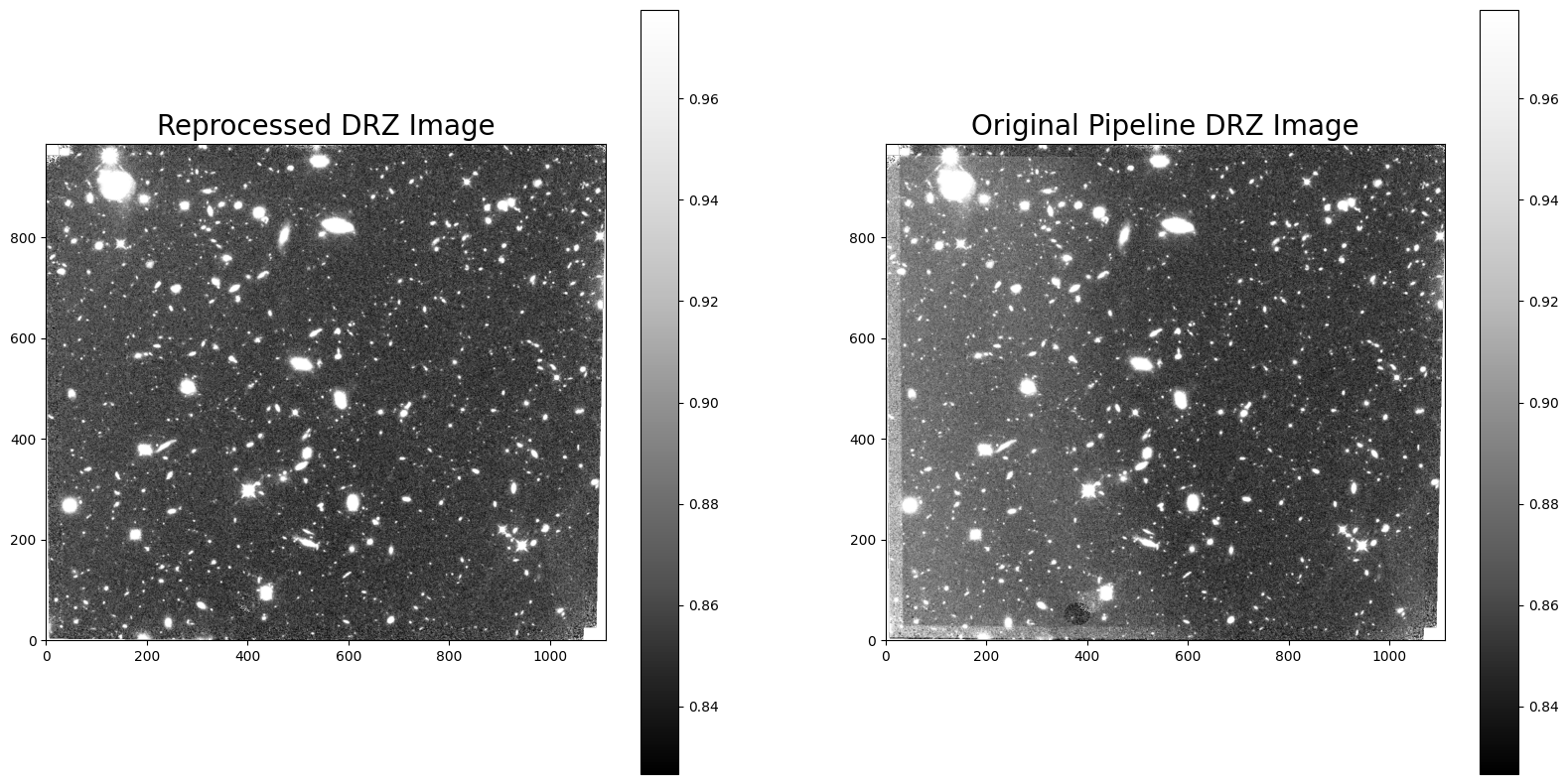
Comparing the new DRZ image made with the reprocessed FLT product against the original pipeline DRZ image, we see that the new DRZ image no longer includes scattered light but has a slightly lower S/N due the reduced total exposure time from 1403 to 1000 seconds.
DRZ_image = fits.getdata("f140w_drz_sci.fits")
Orig_DRZ = fits.getdata('mastDownload/HST/icqtbb020/icqtbb020_drz.fits')

fig = plt.figure(figsize=(20, 10))
rows = 1
columns = 2

# Add the total exptime in the title
ax1 = fig.add_subplot(rows, columns, 1)
ax1.set_title("Reprocessed DRZ Image", fontsize=20)
vmin, vmax = zscale(Orig_DRZ)
im1 = plt.imshow(DRZ_image, vmin=vmin, vmax=vmax, origin='lower', cmap='Greys_r')
_ = plt.colorbar()

ax2 = fig.add_subplot(rows, columns, 2)
ax2.set_title("Original Pipeline DRZ Image", fontsize=20)
im2 = plt.imshow(Orig_DRZ, vmin=vmin, vmax=vmax, origin='lower', cmap='Greys_r')
_ = plt.colorbar()
7. Conclusions #
Congratulations, you have completed the notebook.
You should now be familiar with how to reprocess an observation affected by Earth limb scattered light by removing the affected reads from your science and error images.
Thank you for following along!
Additional Resources #
Below are some additional resources that may be helpful. Please send any questions through the HST Help Desk.
About this Notebook #
Author: Anne O’Connor, Jennifer Mack, Annalisa Calamida, Harish Khandrika – WFC3 Instrument
Updated On: 2023-11-13
Citations #
If you use the following tools for published research, please cite the authors. Follow these links for more information about citing the tools:
If you use this notebook, or information from the WFC3 Data Handbook, Instrument Handbook, or WFC3 ISRs for published research, please cite them:
Citing this notebook: Please cite the primary author and year, and hyperlink the notebook or HST/WFC3 Notebooks
