
Satellite Trail Masking Techniques#
Table of Contents#
1. Download the Observations with astroquery
Introduction #
Even though Hubble has a small field of view, satellites are commonly captured in images. The cosmic ray rejection algorithm in Astrodrizzle is not well suited to eliminate satellite trails, and the affected adjacent pixels that make up their wings leave ugly blemishes in stacked images.
To fix this problem, the pixels around satellite trails need to be marked as bad in the affected images. There are several ways to accomplish this goal. The ACS Team developed multiple algorithms to automatically detect and mask satellite trails. The newest is a module called findsat_mrt and is decribed in ISR ACS 2022-08. The ‘readthedocs’ page can be found here: MRT-based Satellite Trail Detection. The second module is called satdet and is described in ISR ACS 2016-01. The ‘readthedocs’ page for the software can be found here: Satellite Trails Detection. findsat_mrt has the benefit of significantly improved sensitivity over satdet but it is more computationally demanding.
Masks can also be made manually using DS9 regions. While not as convenient, making masks manually allows you to mask not only satellites, but also any other anomalies with odd shapes (e.g. dragon’s breath, glint, blooming).
All of these methods are demonstrated below. To aid users, we have provided examples using both ACS/WFC and WFC3/UVIS imaging data, although most of the tools shown in this notebook can be applied to any imaging data.
Import Modules #
The following Python packages are required to run the Jupyter Notebook:
os - change and make directories
glob - gather lists of filenames
shutil - remove directories and files
matplotlib - make figures and graphics
astropy - file handling, tables, units, WCS, statistics
astroquery - download data and query databases
drizzlepac - align and combine HST images
IPython - to display images
skimage - for image processing
acstools - for HST/ACS image processing
regions - parse DS9 region files
import os
import glob
import shutil

import matplotlib.pyplot as plt
from regions import Regions

from astropy.io import fits
from astroquery.mast import Observations
from astropy.visualization import astropy_mpl_style, ImageNormalize, LinearStretch

from IPython.display import Image, clear_output

from acstools.findsat_mrt import WfcWrapper
from acstools.utils_findsat_mrt import update_dq
from acstools.satdet import detsat, make_mask

from skimage.morphology import dilation
from skimage.morphology import square

from drizzlepac.astrodrizzle import AstroDrizzle as adriz
from drizzlepac.processInput import getMdriztabPars


# configure the plot output
%matplotlib inline
%config InlineBackend.figure_format = 'retina' # Improves the resolution of figures rendered in notebooks.
1. Download the Observations with astroquery #
MAST queries may be done using `query_criteria`, where we specify:
–> obs_id, proposal_id, and filters
MAST data products may be downloaded by using download_products, where we specify:
–> products = calibrated (FLT, FLC) or drizzled (DRZ, DRC) files
–> type = standard products (CALxxx) or advanced products (HAP-SVM)
1.1 Download the ACS data #
The ACS/WFC images to be used are the F814W images of visit B7 from GO program 13498. These come from the Hubble Frontier Fields program and are images of the the galaxy cluster MACSJ0717.5+3745.
The four FLC images have been processed by the HST ACS pipeline (calacs), which includes bias subtraction, dark current correction, cte-correction, cosmic-ray rejection, and flatfielding:
        jc8mb7sqq_flc.fits
        jc8mb7sxq_flc.fits
        jc8mb7t5q_flc.fits
        jc8mb7tcq_flc.fits
Additionally we will download the JPG preview images and keep only the DRC file:
jc8mb7020_drc.jpg
obs_id_acs = 'JC8MB7020'

obsTable = Observations.query_criteria(obs_id=obs_id_acs)
products = Observations.get_product_list(obsTable)

data_type = 'CALACS'                             # ['CALACS','CALWF3','CALWP2','HAP-SVM']
data_prod = 'FLC'                                # ['FLC','FLT','DRC','DRZ']

flc_download = Observations.download_products(products, project=data_type, productSubGroupDescription=data_prod)
jpg_download = Observations.download_products(products, project=data_type, extension=['jpg'])

clear_output()
Move to the files to the local working directory, and print the files
if os.path.exists('mastDownload'):
    for file in jpg_download['Local Path']:
        if 'drc' in file:
            os.rename(file, os.path.basename(file))
    for file in flc_download['Local Path']:
        os.rename(file, os.path.basename(file))
    shutil.rmtree('mastDownload')
list = sorted(glob.glob('j*.*'))
list
['jc8mb7020_drc.jpg',
 'jc8mb7sqq_flc.fits',
 'jc8mb7sxq_flc.fits',
 'jc8mb7t5q_flc.fits',
 'jc8mb7tcq_flc.fits']
1.2 Download the WFC3 data #
The WFC3/UVIS images to be used are F350LP images from visit 11 of NGC 4051 from GO program 14697.
The three FLC images have been processed by the HST WFC3 pipeline (calwf3), which includes bias subtraction, dark current correction, cte-correction, cosmic-ray rejection, and flatfielding.
        id8m11g1q_flc.fits
        id8m11g2q_flc.fits
        id8m11g4q_flc.fits
Additionally we will download the JPG preview images and keep only the DRC file:
id8m11010_drc.jpg
obs_id_wfc3 = 'ID8M11010'

obsTable = Observations.query_criteria(obs_id=obs_id_wfc3)
products = Observations.get_product_list(obsTable)

data_type = ['CALWF3']                             # ['CALACS','CALWF3','CALWP2','HAP-SVM']
data_prod = ['FLC']                                # ['FLC','FLT','DRC','DRZ']

flc_download = Observations.download_products(products, project=data_type, productSubGroupDescription=data_prod)
jpg_download = Observations.download_products(products, project=data_type, extension=['jpg'])

clear_output()
Move to the files to the local working directory, and print them
if os.path.exists('mastDownload'):
    for file in jpg_download['Local Path']:
        if 'drc' in file:
            os.rename(file, os.path.basename(file))
    for file in flc_download['Local Path']:
        os.rename(file, os.path.basename(file))
    shutil.rmtree('mastDownload')
list = sorted(glob.glob('i*.*'))
list
['id8m11010_drc.jpg',
 'id8m11g1q_flc.fits',
 'id8m11g2q_flc.fits',
 'id8m11g4q_flc.fits']
2. ACS/WFC Example #
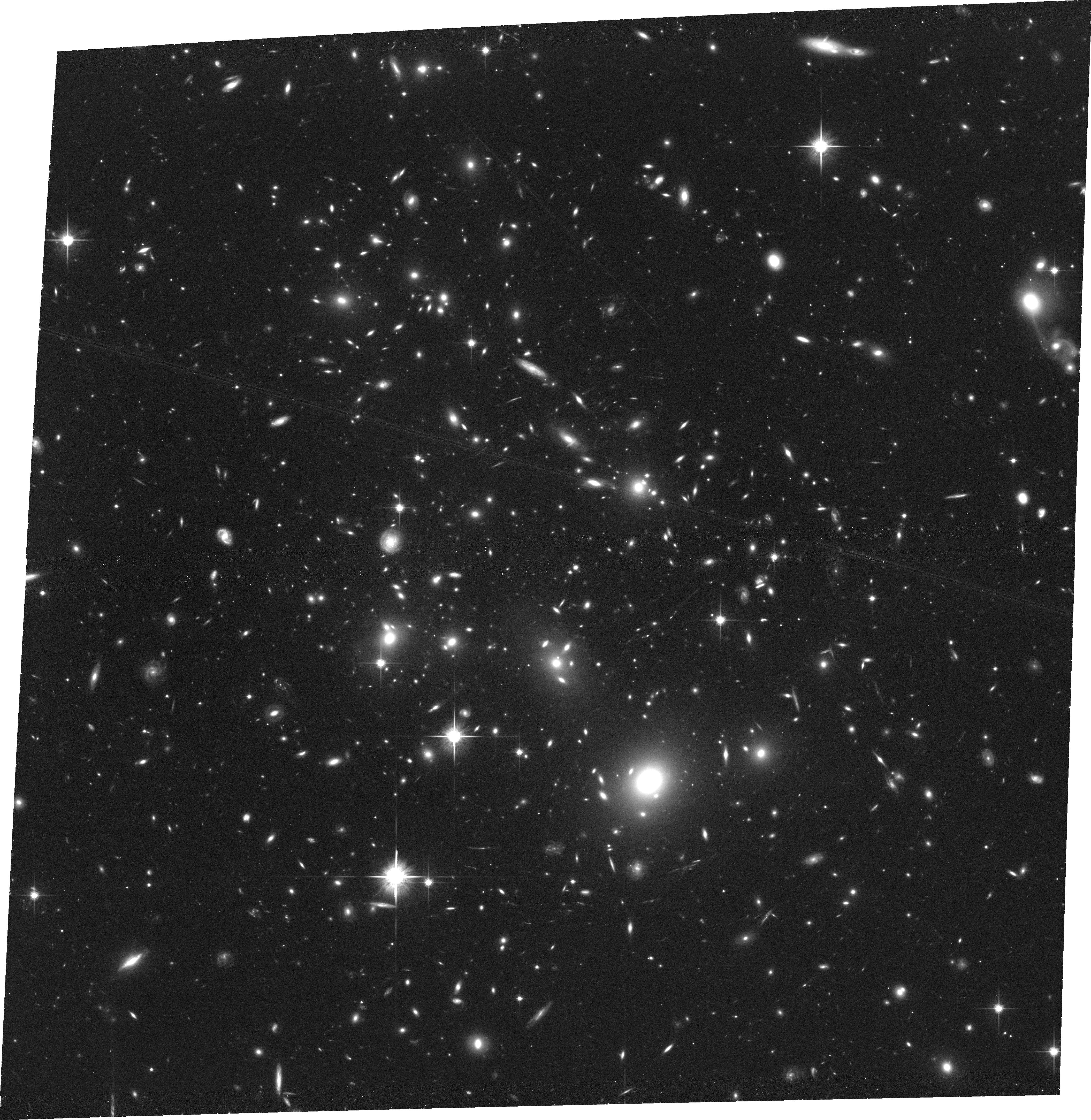
The image below shows the combined drizzled image from this association. The satellite trail can be seen going across the image from left to right, just above the center of the image. It is partially masked by the routines in Drizzlepac that mask cosmic rays, but the wings of the satellite trail are still noticeable.
Image(filename=obs_id_acs.lower() + '_drc.jpg', width=800, height=800)
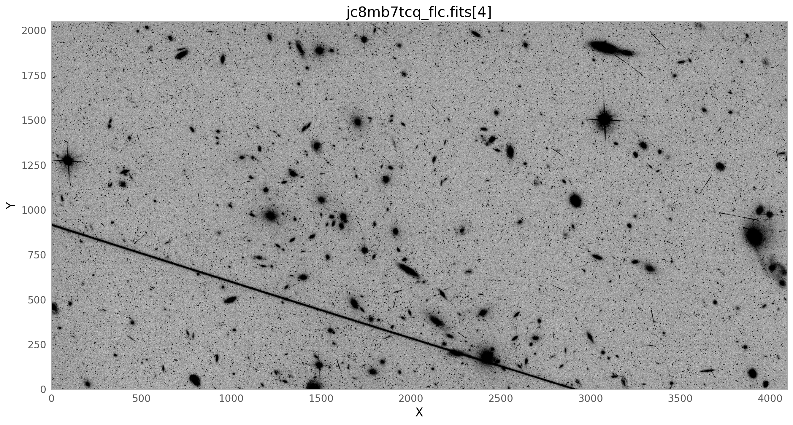
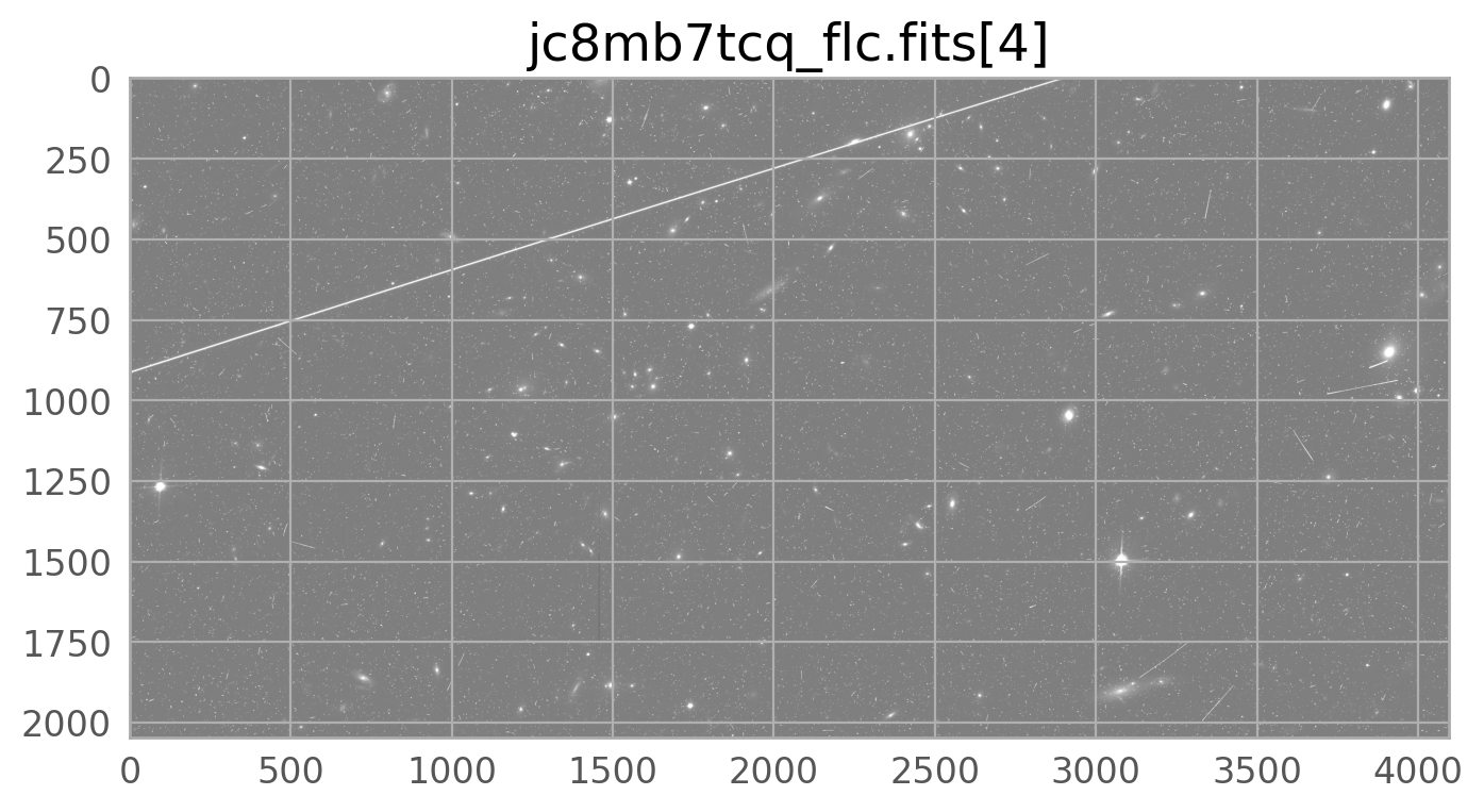
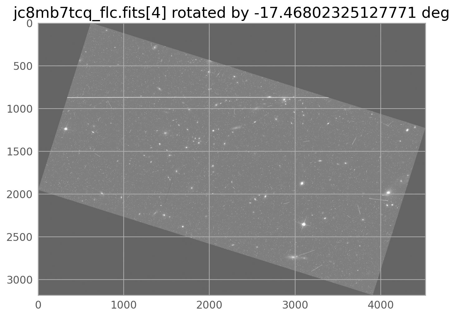
The bright satellite trail that caused this came from the image jc8mb7cq_flc.fits. The figure below shows the top chip which is referred to as SCI,2 (or extension 4).
flc_file = 'jc8mb7tcq_flc.fits' # defining this variable since we'll use it a lot
img = fits.getdata(flc_file, ext=4)
plt.style.use(astropy_mpl_style)

norm1 = ImageNormalize(img, vmin=100, vmax=200, stretch=LinearStretch())
fig, ax = plt.subplots(figsize=(16, 16))
c = ax.imshow(img, norm=norm1, cmap='gray_r', origin='lower')
ax.set_xlabel('X')
ax.set_ylabel('Y')
ax.set_title(flc_file+'[4]')
plt.grid()
2.1 Option A: Using findsat_mrt #
The WfcWrapper class provides a simple one-line approach to creating a mask for satellite trails. In this example, we run WfcWrapper on the top chip only (SCI,1 or extension 4). WfcWrapper loads the data, prepares the image (applies rebinning, removes a background, and masks already identified bad pixels), and executes the detection routines. In this example, we rebin the data by 2 pixels in each direction and use 8 processes. You may want to adjust the binning and/or number of processes depending on your system. We also set a maximum trail width of 75 pixels (this can also be adjusted depending on your binning).
w = WfcWrapper(flc_file,
               extension=4,
               binsize=2,
               processes=8,
               max_width=75,
               preprocess=True,
               execute=True)

clear_output()
We can plot the mask on its own, or overlaid on the input image.
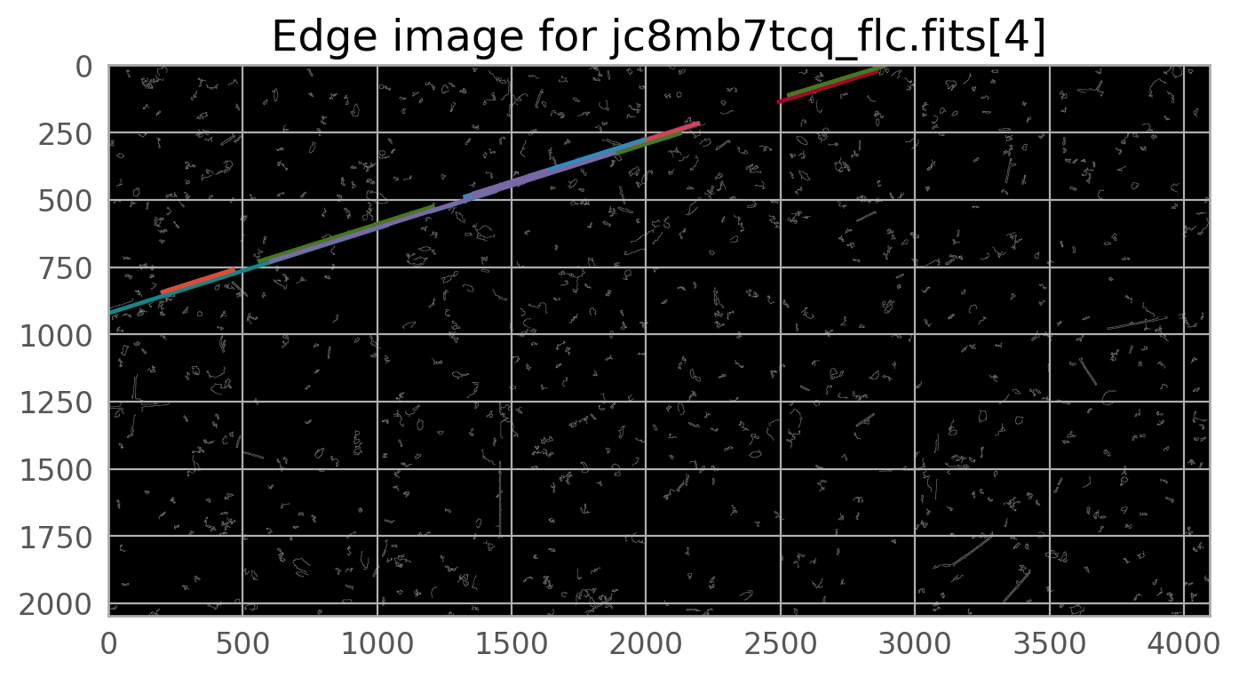
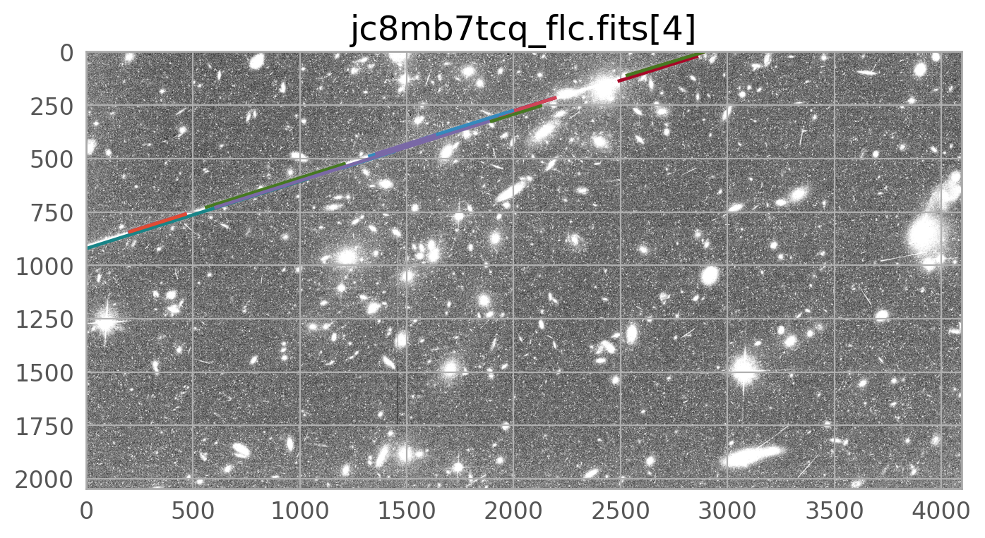
w.plot_mask()
w.plot_image(overlay_mask=True)
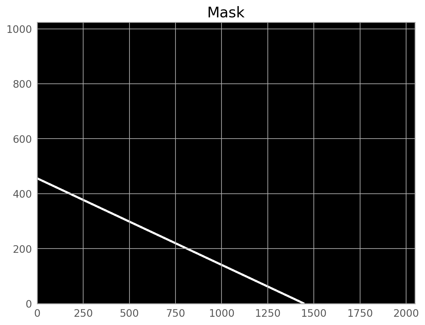
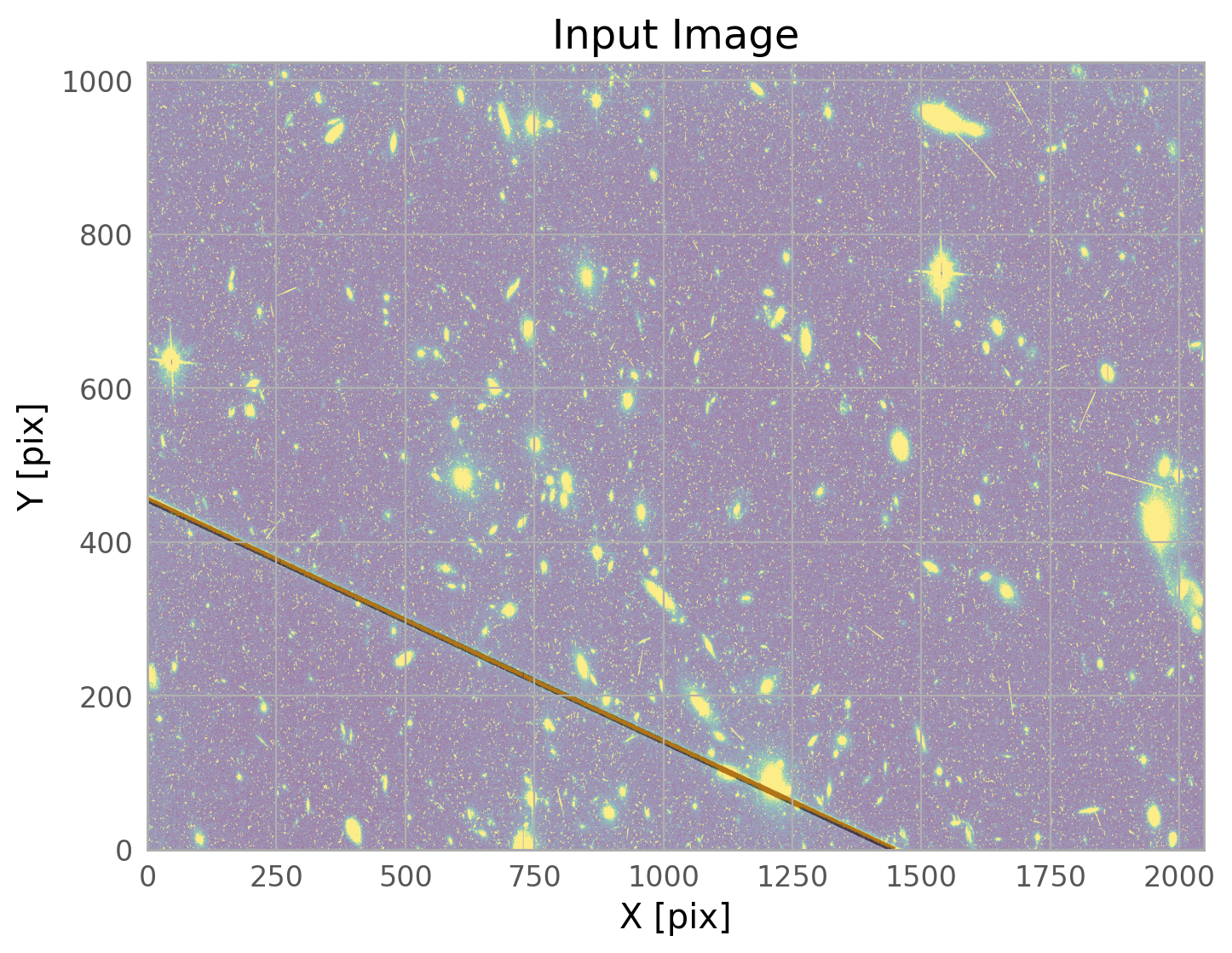
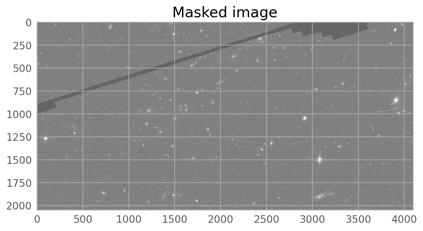
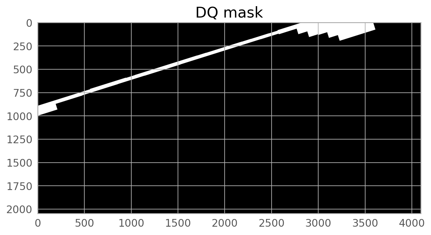
We clearly see the mask covering the satellite trail. The call to WfcWrapper above works well for most ACS/WFC data, but if you want to adjust the parameters, please see the documentation for acstools.findsat_mrt.
The mask created by WfcWrapper casts a pretty wide net around the trail it finds, but there may be situations where you need to broaden it further, especially for very bright satellite trails. The skimage.morphology.dilation routine is one way to do this.
mask_mrt = dilation(w.mask, square(10))  # adjust the box size to whatever you need
w.mask = mask_mrt  # update the mask attribute in the WfcWrapper instance
WARNING:py.warnings:/tmp/ipykernel_3604/2861942194.py:1: FutureWarning: `square` is deprecated since version 0.25 and will be removed in version 0.27. Use `skimage.morphology.footprint_rectangle` instead.
  mask_mrt = dilation(w.mask, square(10))  # adjust the box size to whatever you need
It is important to keep in mind that the mask we have created has the dimensions of the binned input image. It will need to be expanded before it can be used. This will be done in a later step
2.2 Option B: Using satdet #
The first command below runs the detection algorithm on the top chip only (extension 4) and generates some diagnostic plots. Note that the images are shown upside down from the figure above.
results, errors = detsat(flc_file,
                         chips=[4],
                         n_processes=4,
                         plot=True,
                         verbose=True)
clear_output()
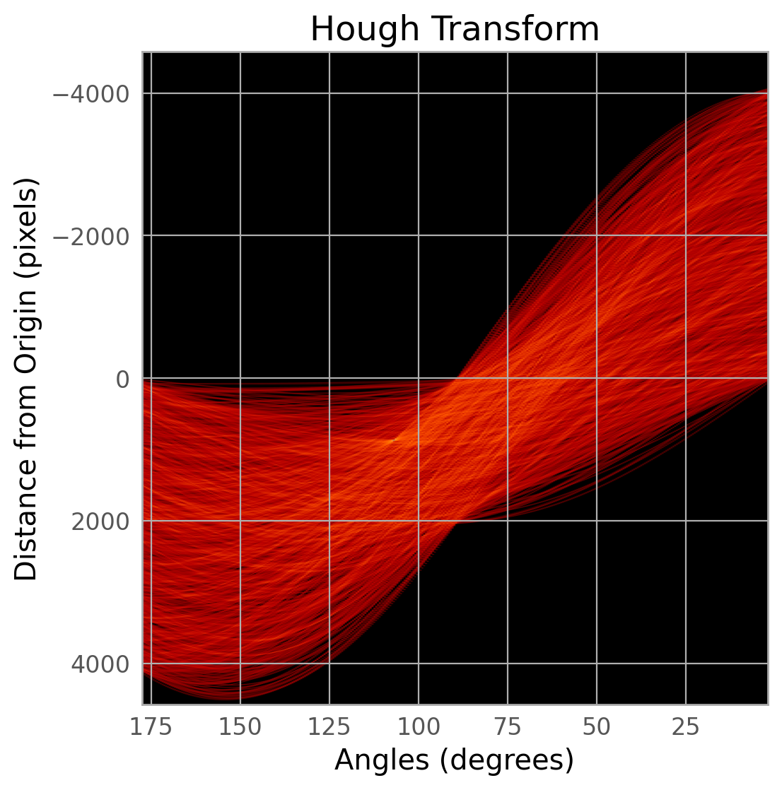
The diagnostic plots can be used to verify that the satellite was properly detected. Changing parameters to adjust this task is beyond the scope of this notebook, but please consult the package documentation indicated above for instructions on how to do this.
Assuming that the satellite trail was properly detected, masks can be made to flag the satellite in the data quality array (DQ) of the image. Below, we generate the satellite trail mask. The DQ array is updated in a later step.
trail_coords = results[(flc_file, 4)]
trail_segment = trail_coords[0]
trail_segment
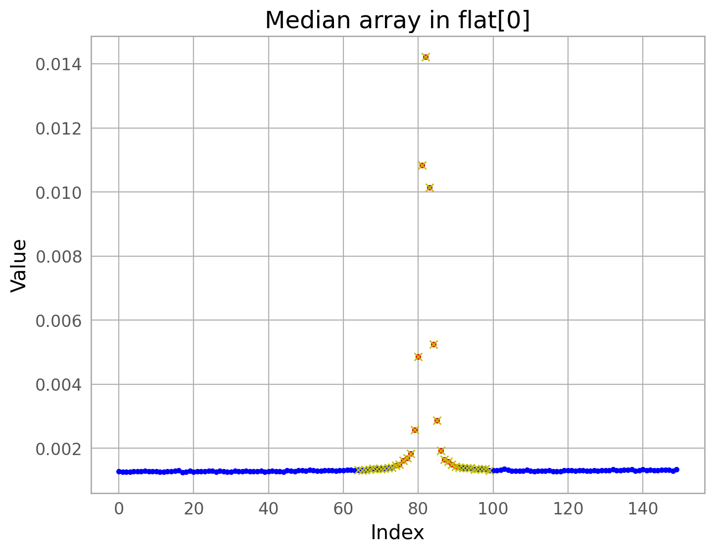
mask_satdet = make_mask(flc_file, 4, trail_segment, plot=True, verbose=True)
Rotation: -17.46802325127771
No good profile found for counter=20. Start moving left from starting point.
z=[] is less than 1, subr shape=(150, 200), we are done
Run time: 2.3255362510681152 s
2.3 Running AstroDrizzle #
The next step is to run AstroDrizzle to combine the flc files into a final image, but first, we need to update the DQ array in the input fits file that contained the satellite trail. Once this information is in the DQ array, AstroDrizzle knows to ignore the flagged pixels when making the combined image. Below is one possible command to update the DQ array with one of the masks we created above using the update_dq, which sets the flagged pixels to 16384 in the DQ array. By default, we use the mask generated by findsat_mrt, but this can be changed. Note that if using the mask created by findsat_mrt, which was generated on a binned image, update_dq will automatically expand it to the original image dimensions.
Here, we are updating pixels in the DQ array of SCI,2 (extension 6). If we were flagging a satellite on the bottom chip (SCI,1 or extension 1), the update_dq function would instead be used to modify extension 3. More detail on the ACS file structure may be found in the ACS Data Handbook.
final_mask = mask_mrt       # uncomment this line to use the mask from findsat_mrt
# final_mask = mask_satdet  # uncomment this line to use the mask from satdet

update_dq(flc_file, 6, final_mask, verbose=True, expand_mask=True)

# note: if running findsat_mrt, you could also update the DQ array with:
# w.updatedq()
INFO:utils_findsat_mrt:Inconsistent mask sizes:
Input mask: (1024, 2048)
DQ array: (2048, 4096)
INFO:utils_findsat_mrt:Enlarging mask to original size.
DQ flag value is 16384
Input... flagged NPIX=116576
Existing flagged NPIX=0
Newly... flagged NPIX=116576
jc8mb7tcq_flc.fits[6] updated
With the satellite masked, the images can be drizzled again. For brevity, only the top chip (SCI,2) of the image stack will be drizzled together to make a combined product. This is controlled in AstroDrizzle via the group parameter.
Here, we get some recommended values for drizzling from the MDRIZTAB reference file. The parameters in this file are different for each detector and are based on the number of input frames. These are a good starting point for drizzling and may be adjusted accordingly.
# Set the locations of reference files to your local computer.
os.environ['CRDS_SERVER_URL'] = 'https://hst-crds.stsci.edu'
os.environ['CRDS_SERVER'] = 'https://hst-crds.stsci.edu'
os.environ['CRDS_PATH'] = './crds_cache'
os.environ['iref'] = './crds_cache/references/hst/wfc3/'
os.environ['jref'] = './crds_cache/references/hst/acs/'
# The following lines of code find and download the MDRIZTAB reference file.
input_images = sorted(glob.glob('j*_flc.fits'))

mdz = fits.getval(input_images[0], 'MDRIZTAB', ext=0).split('$')[1]
print('Searching for the MDRIZTAB file:', mdz)
!crds sync --hst --files {mdz} --output-dir {os.environ['jref']}
Searching for the MDRIZTAB file: 37g1550cj_mdz.fits
CRDS - INFO -  Symbolic context 'hst-latest' resolves to 'hst_1297.pmap'
CRDS - INFO -  Reorganizing 0 references from 'instrument' to 'flat'
CRDS - INFO -  Reorganizing from 'instrument' to 'flat' cache,  removing instrument directories.
CRDS - INFO -  Syncing explicitly listed files.
CRDS - INFO -  0 errors
CRDS - INFO -  0 warnings
CRDS - INFO -  4 infos
input_images = sorted(glob.glob('j*_flc.fits'))


def get_vals_from_mdriztab(input_images, kw_list=['driz_sep_bits',
                                                  'combine_type',
                                                  'driz_cr_snr',
                                                  'driz_cr_scale',
                                                  'final_bits']):
    '''Get only selected parameters from. the MDRIZTAB'''

    mdriz_dict = getMdriztabPars(input_images)

    requested_params = {}

    print('Outputting the following parameters:')
    for k in kw_list:
        requested_params[k] = mdriz_dict[k]
        print(k, mdriz_dict[k])

    return requested_params
selected_params = get_vals_from_mdriztab(input_images)
- MDRIZTAB: AstroDrizzle parameters read from row 3.
Outputting the following parameters:
driz_sep_bits 336
combine_type median
driz_cr_snr 3.5 3.0
driz_cr_scale 1.5 1.2
final_bits 336
Note that the parameter final_bits= ‘336’ is equivalend to final_bits= ‘256, 64, 16’
We can now the drizzling step and show the output.
# To override any of the above values, e.g.,
# selected_params['final_bits']    = '64, 32'    #to treat saturated pixels 256 as bad and fill with NaN
# selected_params['driz_cr_snr']   = '4.0 3.5'   #less aggressive cr-rejection threshold

adriz(input_images,
      output='automatic',
      group='4',
      preserve=False,
      clean=True,
      build=False,
      context=False,
      skymethod='match',
      **selected_params)

clear_output()
# Display the combined science and weight images

sci = fits.getdata('automatic_drc_sci.fits')
wht = fits.getdata('automatic_drc_wht.fits')

fig = plt.figure(figsize=(15, 15))
ax1 = fig.add_subplot(2, 1, 1)
ax2 = fig.add_subplot(2, 1, 2)

ax1.imshow(sci, vmin=0.09, vmax=0.15, cmap='Greys_r', origin='lower')
ax1.set_xlabel('X')
ax1.set_ylabel('Y')
ax1.set_title('Drizzled science image')
ax2.imshow(wht, vmin=2000, vmax=5000, cmap='Greys_r', origin='lower')
ax2.set_xlabel('X')
ax2.set_xlabel('Y')
ax2.set_title('Drizzled weight image')
Text(0.5, 1.0, 'Drizzled weight image')
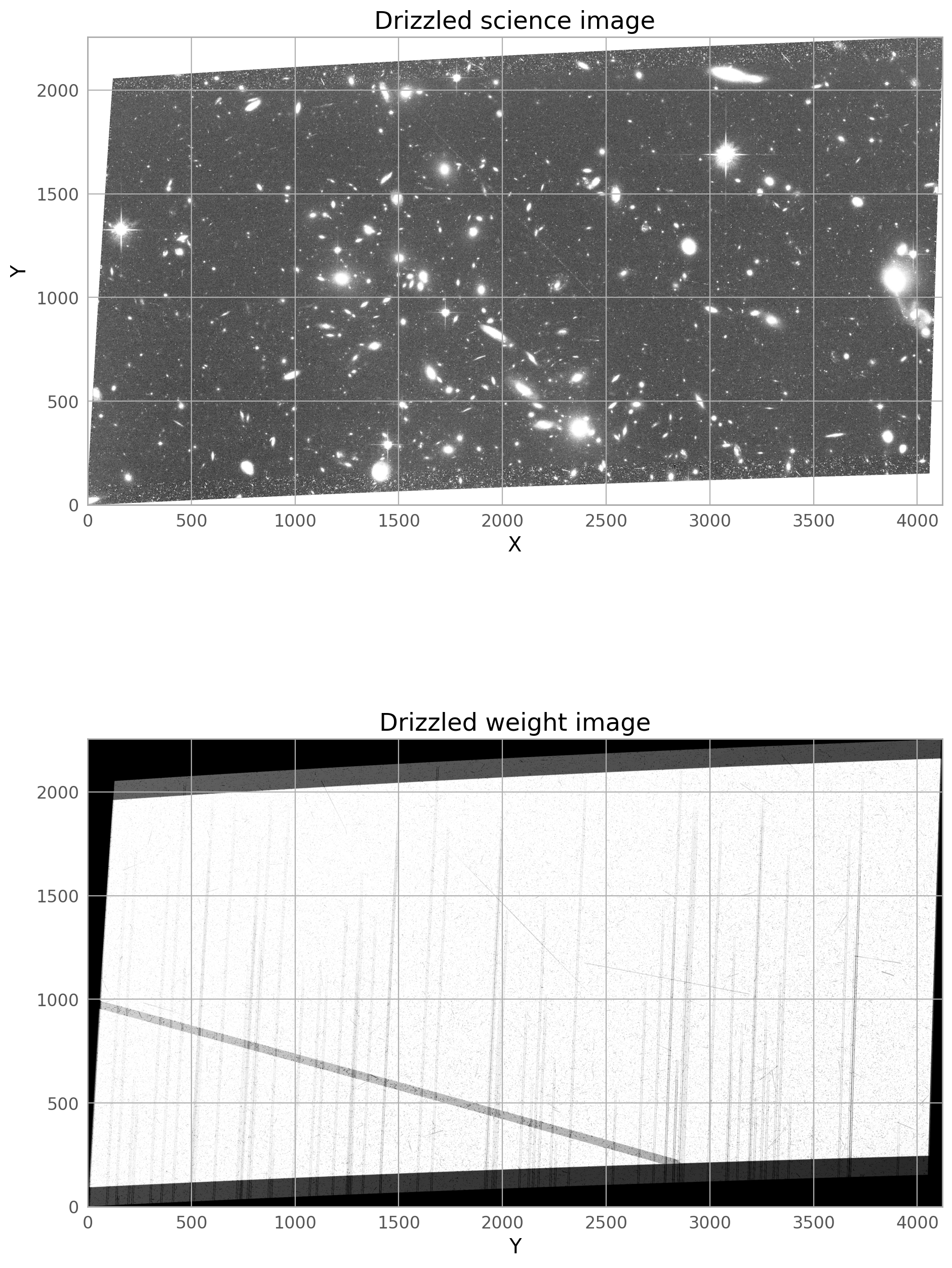
The final drizzled product shows that the bright satellite trail and its wings have been removed. If you don’t see the full trail removed, you may need to broaden the dilate the trail further, and make sure only the four original j*_flc.fits images are getting incorporated into the drizzled image (if you are rerunning AstroDrizzle and are not careful with the inputs, files from previous runs could be used by accident).
A second, fainter satellite can be seen from a different image in the stack, and this will be masked in the steps below.
2.4. Manual masking of satellites and other anomalies #
While the automatic detection algorithm flagged and masked the large satellite trail, the image above shows a second trail from a different image in the stack.
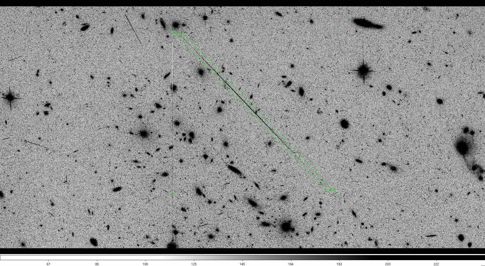
To get rid of this trail, we will demonstrate how a DS9 regions can be used. The example image displayed below shows a region around a satellite trail.
This region was saved in image coordinates. NOTE THAT REGIONS SAVED IN SKY COORDINATES WILL NOT WORK FOR THIS EXAMPLE. Below is the contents of the region file.
# Region file format: DS9 version 4.1
global color=green dashlist=8 3 width=1 font="helvetica 10 normal roman" select=1 highlite=1 dash=0 fixed=0 edit=1 move=1 delete=1 include=1 source=1
image
polygon(1476.9255,1816.4415,1545.7465,1818.5921,2825.3869,485.1853,2765.1685,480.88399)
The regions package will be used to make masks out of region files. For details on how to use this package go here.
Image(filename='sat.jpeg')
# Reading region file
region_string = '''# Region file format: DS9 version 4.1
global color=green dashlist=8 3 width=1 font="helvetica 10 normal roman" select=1 highlite=1 dash=0 fixed=0 edit=1 move=1 delete=1 include=1 source=1
image
polygon(1476.9255,1816.4415,1545.7465,1818.5921,2825.3869,485.1853,2765.1685,480.88399)'''
region1 = Regions.parse(region_string, format='ds9')[0]
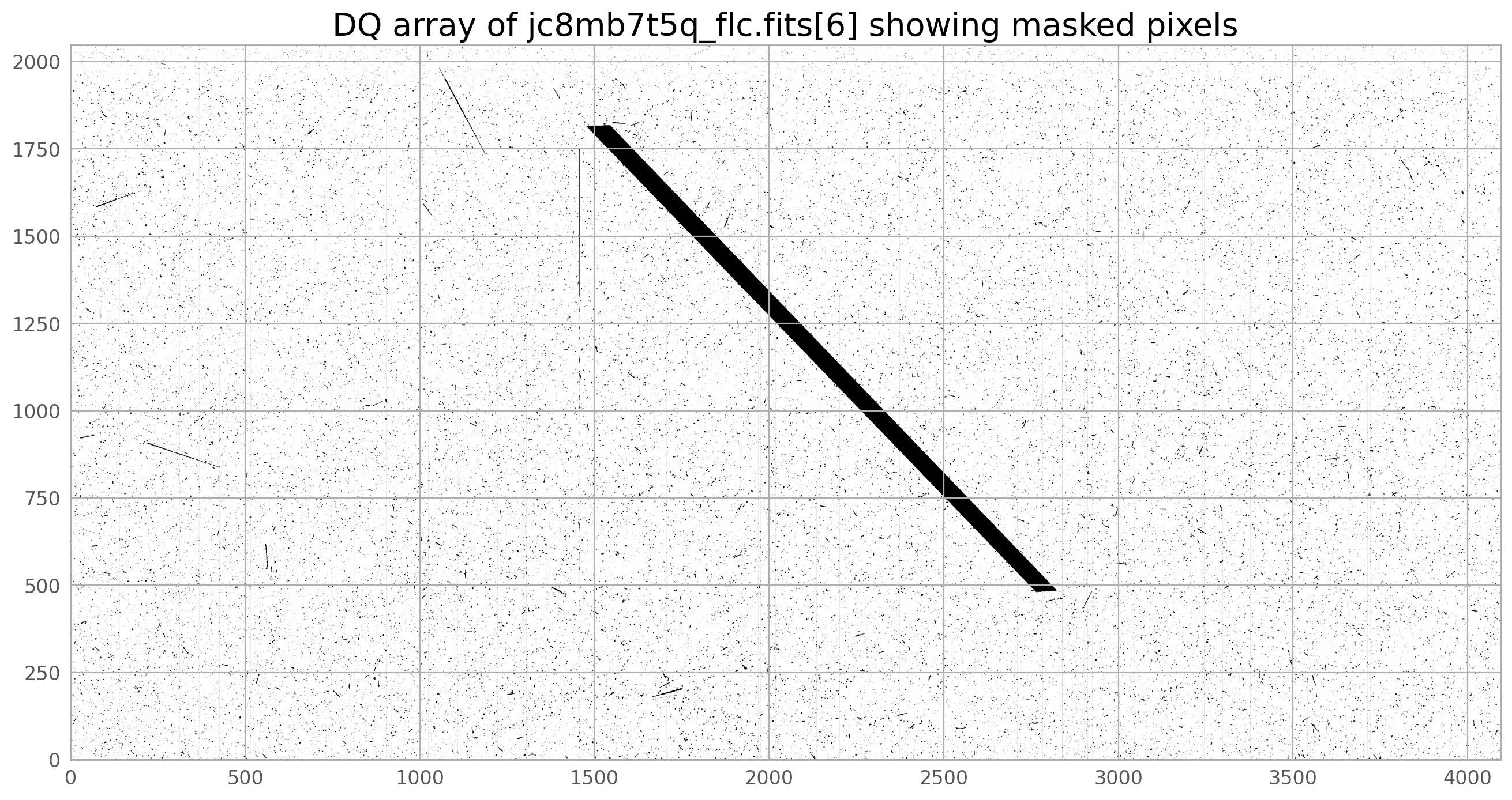
# Making mask out of region file and masking DQ array
with fits.open('jc8mb7t5q_flc.fits', mode='update') as hdu:
dq = hdu[6].data
mask = region1.to_mask().to_image(dq.shape)
mask = mask.astype(bool)
dq[mask] |= 16384
norm1 = ImageNormalize(img, vmin=0, vmax=1000, stretch=LinearStretch())
plt.figure(figsize=(16, 10))
plt.imshow(dq, norm=norm1, cmap='gray_r', origin='lower')
plt.title('DQ array of jc8mb7t5q_flc.fits[6] showing masked pixels', fontsize=20)
Text(0.5, 1.0, 'DQ array of jc8mb7t5q_flc.fits[6] showing masked pixels')
With the satellite masked, the full set of images can be drizzled once more.
adriz(input_images,
      output='manual',
      group='4',
      preserve=False,
      clean=True,
      build=False,
      context=False,
      skymethod='match',
      **selected_params)

clear_output()
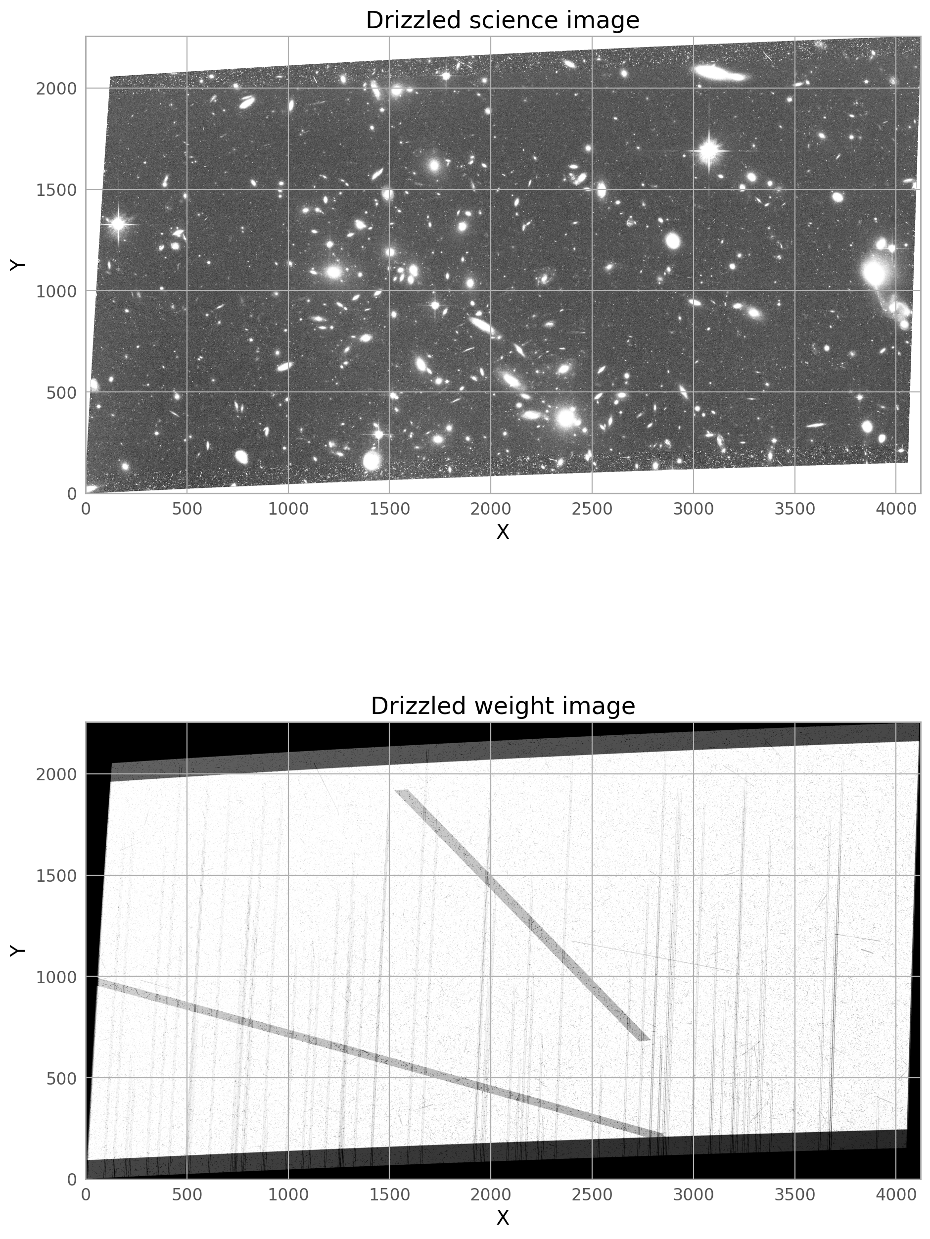
The new drizzled product shows that the second satellite trail and its wings have been removed.
# Display the combined science and weight images

sci = fits.getdata('manual_drc_sci.fits')
wht = fits.getdata('manual_drc_wht.fits')

fig = plt.figure(figsize=(15, 15))
ax1 = fig.add_subplot(2, 1, 1)
ax2 = fig.add_subplot(2, 1, 2)

ax1.imshow(sci, vmin=0.09, vmax=0.15, cmap='Greys_r', origin='lower')
ax1.set_xlabel('X')
ax1.set_ylabel('Y')
ax1.set_title('Drizzled science image')
ax2.imshow(wht, vmin=2000, vmax=5000, cmap='Greys_r', origin='lower')
ax2.set_xlabel('X')
ax2.set_ylabel('Y')
ax2.set_title('Drizzled weight image')
Text(0.5, 1.0, 'Drizzled weight image')
3. WFC3/UVIS Example #
The WFC3/UVIS images to be used are F350LP images from visit 11 of NGC 4051 from GO program 14697.
Although the both findsat_mrt and satdet were initially designed for use with ACS/WFC imaging data, they both also work well for WFC3/UVIS data. Thanks for the similar file structure, most calls to these programs are identical to the example above aside from modifying the file names.
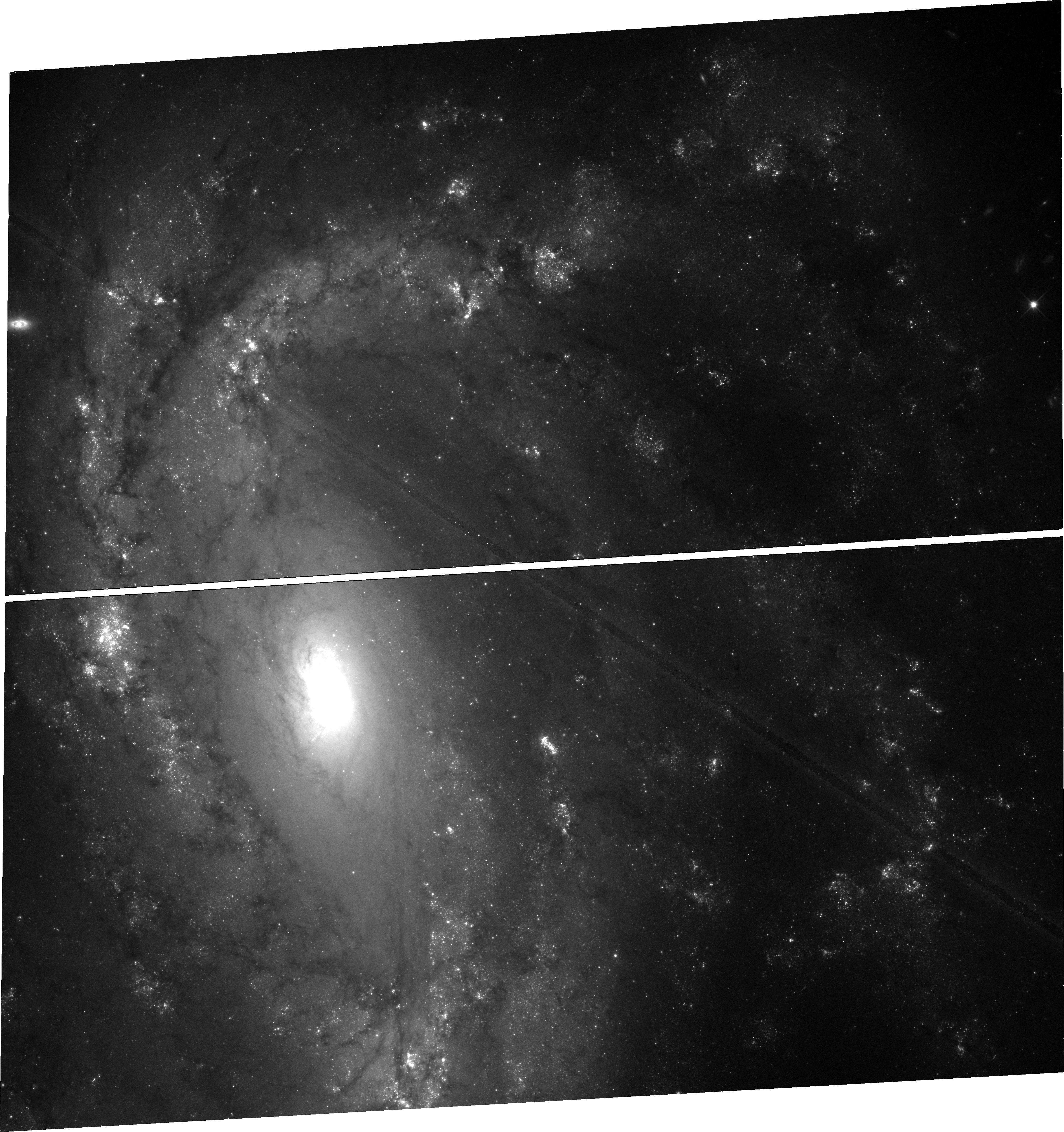
The image below shows the combined drizzled image from this association. The satellite trail can be seen going across the image from left to right. It is partially masked by the routines in Drizzlepac that mask cosmic rays, but the wings of the satellite trail are still noticeable.
Image(filename=obs_id_wfc3.lower() + '_drc.jpg', width=800, height=800)
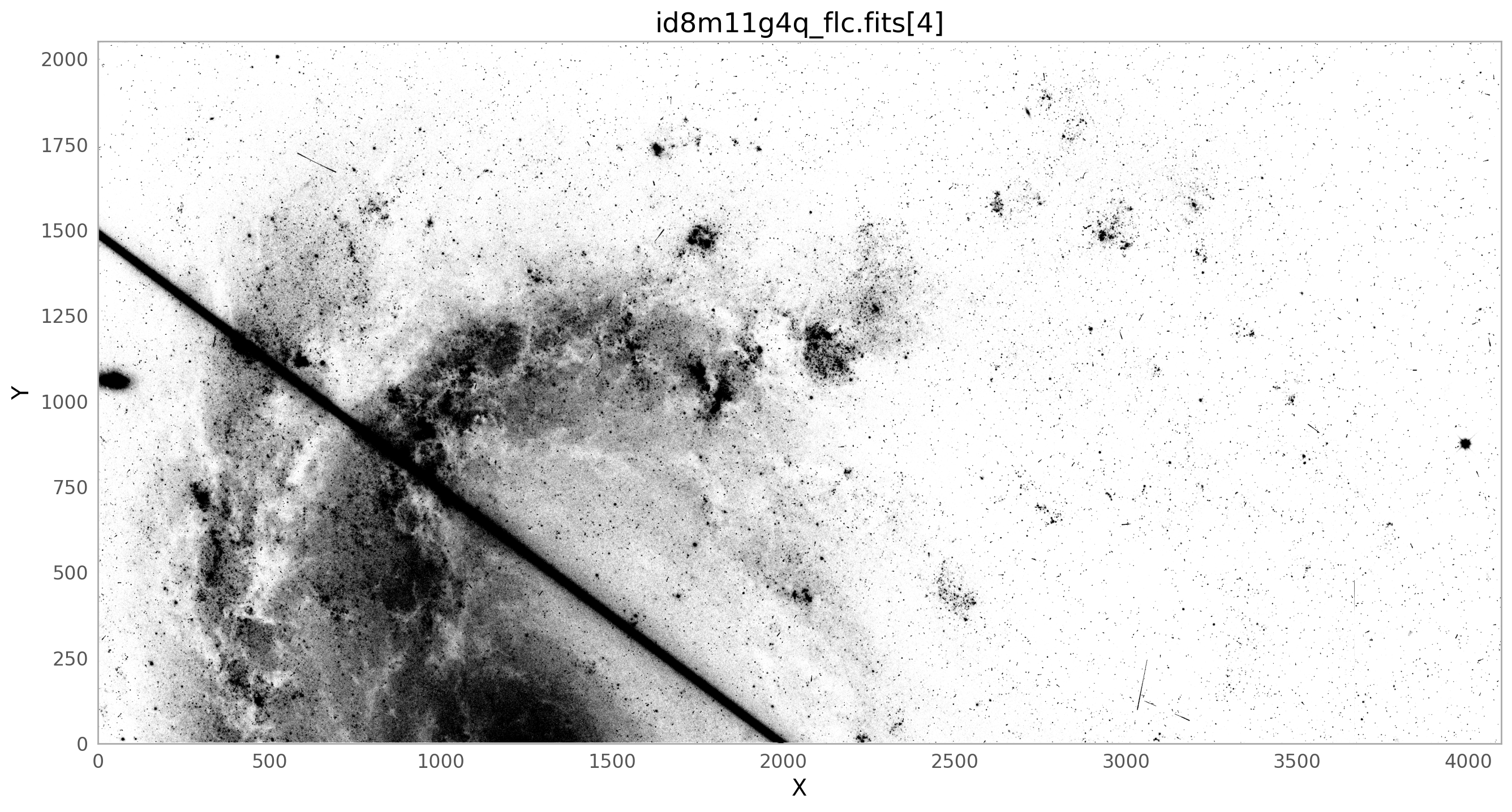
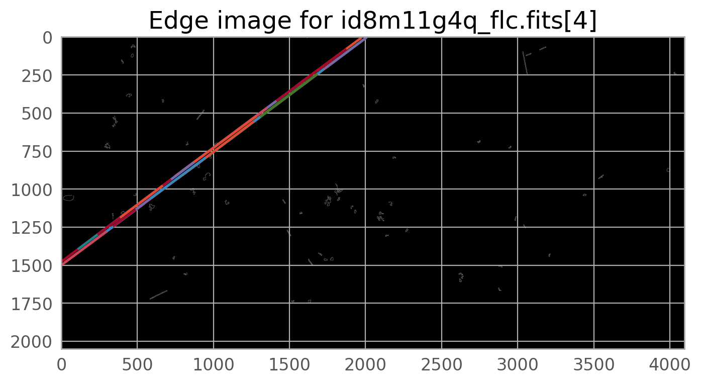
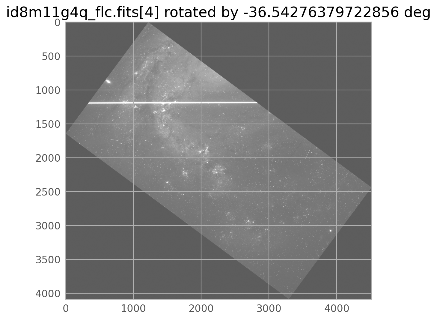
The bright satellite trail that caused this came from the image id8m11g4q_flc.fits. The figure below shows the top chip which is referred to as SCI,2 (or extension 4).
flc_file = 'id8m11g4q_flc.fits' # defining this variable since we'll use it a lot
plt.style.use(astropy_mpl_style)
img = fits.getdata(flc_file, ext=4)

norm1 = ImageNormalize(img, vmin=100, vmax=200, stretch=LinearStretch())
fig, ax = plt.subplots(figsize=(16, 16))
c = ax.imshow(img, norm=norm1, cmap='gray_r', origin='lower')
ax.set_xlabel('X')
ax.set_ylabel('Y')
ax.set_title(flc_file+'[4]')
plt.grid()
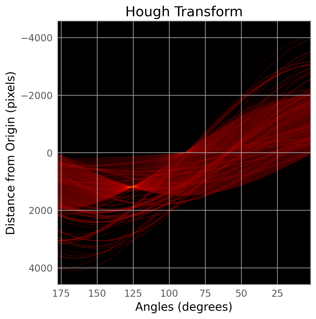
3.1 Option A: Using findsat_mrt #
The WfcWrapper class is designed to make processing of ACS/WFC data quick and easy, but thanks for the identical file structure for WFC3/UVIS data, we can use this functionality again. In this example, we run WfcWrapper on the top chip only (SCI,1 or extension 4). WfcWrapper loads the data, prepares the image (applies rebinning, removes a background, and masks already identified bad pixels), and executes the detection routines. In this example, we rebin the data by 2 pixels in each direction and use 8 processes. You may want to adjust the binning and/or number of processes depending on your system. We also set a maximum trail width of 75 pixels (this can also be adjusted depending on your binning).
w = WfcWrapper(flc_file,
               extension=4,
               binsize=2,
               processes=8,
               max_width=75,
               preprocess=True,
               execute=True)

clear_output()
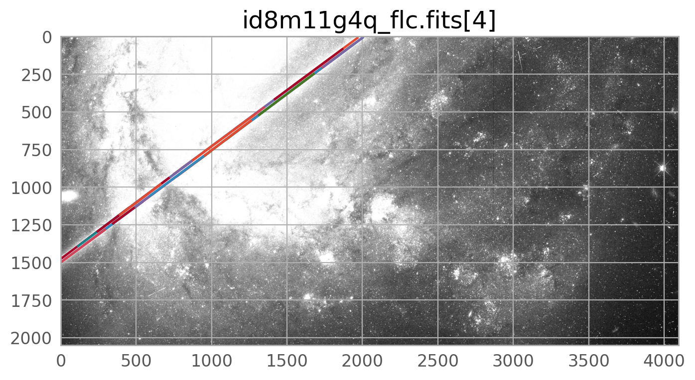
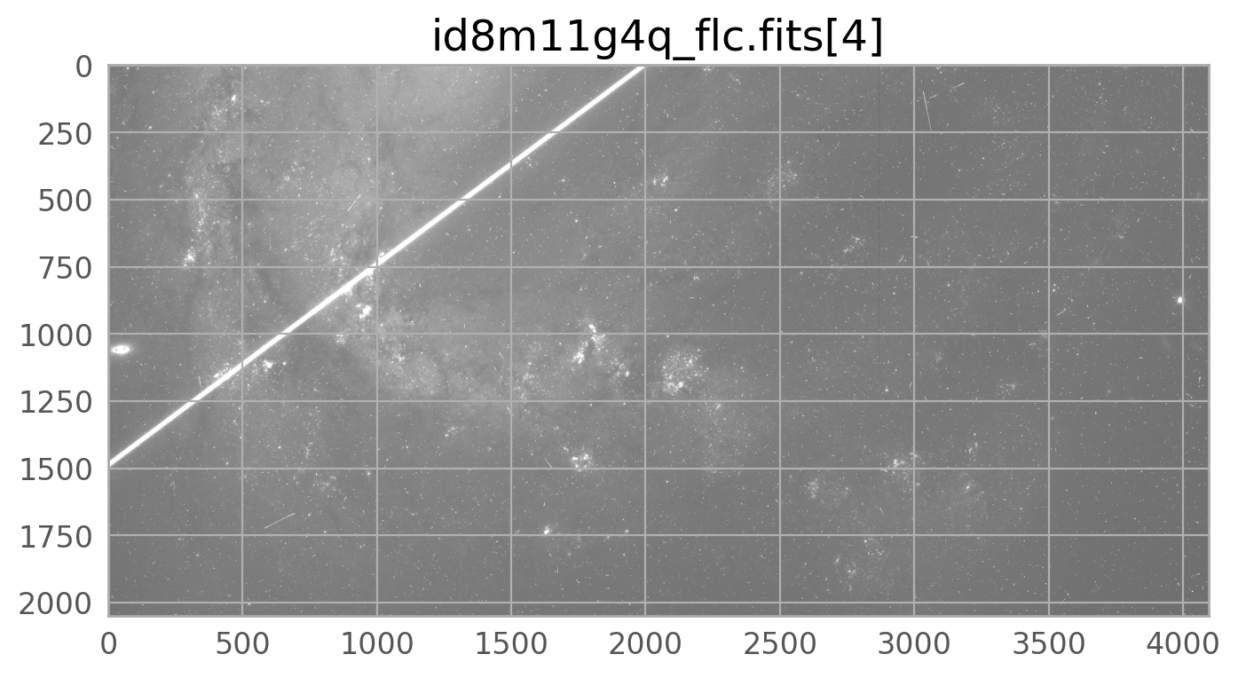
We can plot the mask on its own, or overlaid on the input image, where it can be seen on top of the input image
w.plot_mask()
w.plot_image(overlay_mask=True)
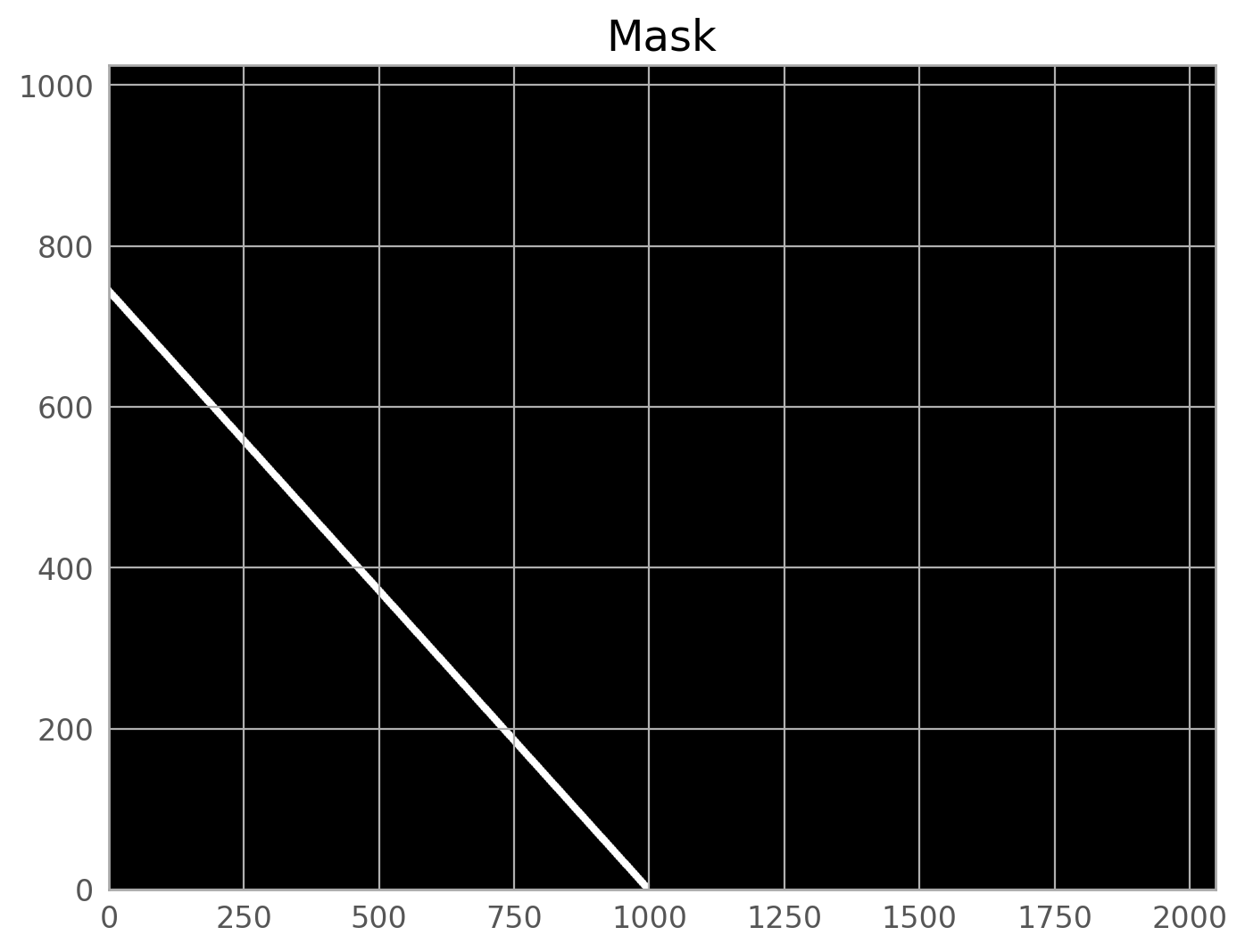
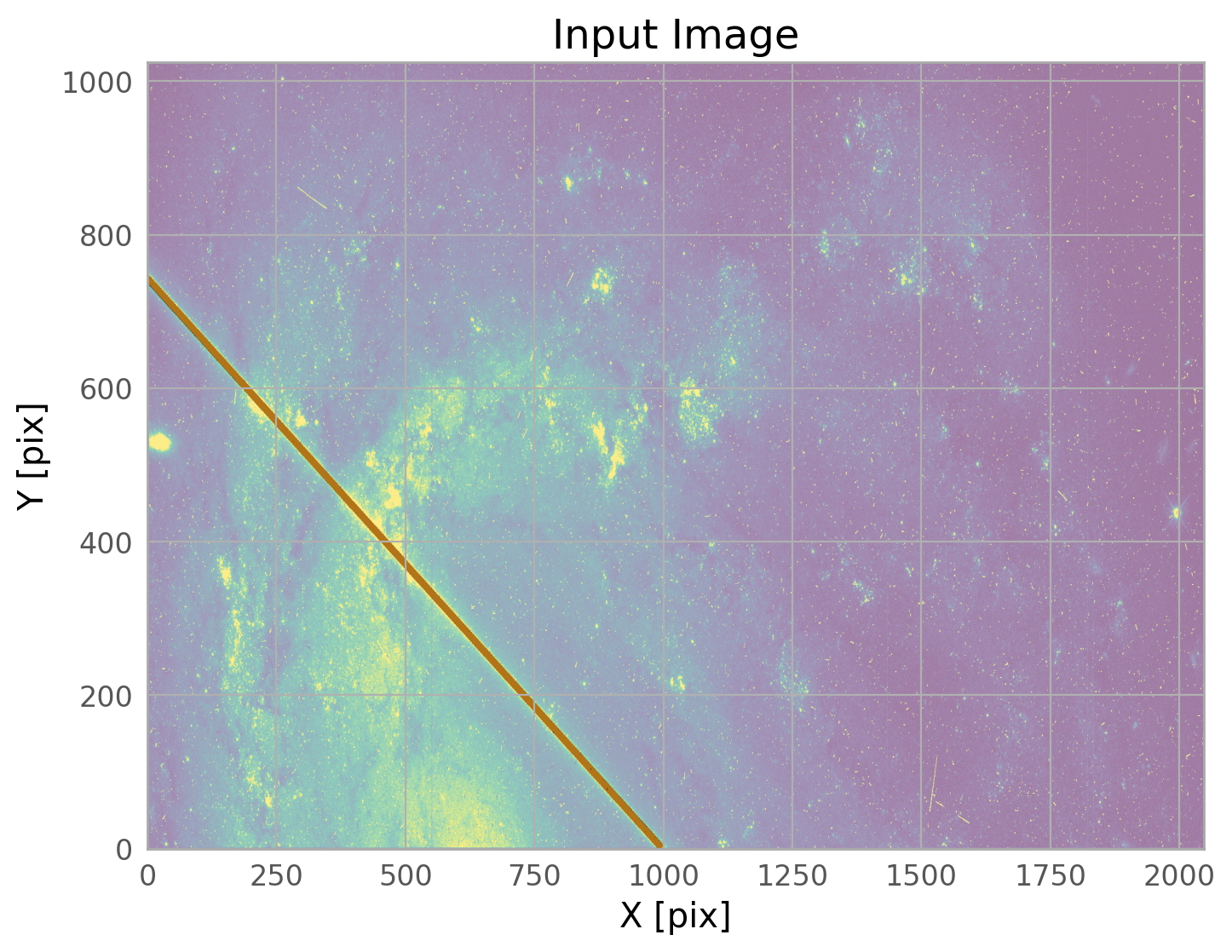
The mask created by WfcWrapper casts a pretty wide net around the trail it finds, but there may be situations where you need to broaden it further, especially for very bright satellite trails. The skimage.morphology.dilation is one way to do this.
mask_mrt = dilation(w.mask, square(20))  # adjust the box size to whatever you need
w.mask = mask_mrt                       # update the mask attribute in the WfcWrapper instance
/tmp/ipykernel_3604/1969779303.py:1: FutureWarning: `square` is deprecated since version 0.25 and will be removed in version 0.27. Use `skimage.morphology.footprint_rectangle` instead.
  mask_mrt = dilation(w.mask, square(20))  # adjust the box size to whatever you need
It is important to keep in mind that the mask we have created has the dimensions of the binned input image. It will need to be expanded before it can be used. This will be done in a later step.
3.2 Option B: Using satdet #
The first command below runs the detection algorithm on the top chip only (extension 4) and generates some diagnostic plots. Note that the images are shown upside down from the figure above.
results, errors = detsat(flc_file,
                         chips=[4],
                         n_processes=4,
                         plot=True,
                         verbose=True,
                         percentile=(1, 99))
clear_output()
The diagnostic plots can be used to verify that the satellite was properly detected. Further changing the parameters to adjust this task is beyond the scope of this notebook, but please consult the package documentation indicated above for instructions on how to do this.
Assuming that the satellite trail was properly detected, masks can be made to flag the satellite in the data quality array (DQ) of the image. Below, we generate the satellite trail mask. The DQ array is updated in a later step.
trail_coords = results[(flc_file, 4)]
trail_segment = trail_coords[0]
trail_segment
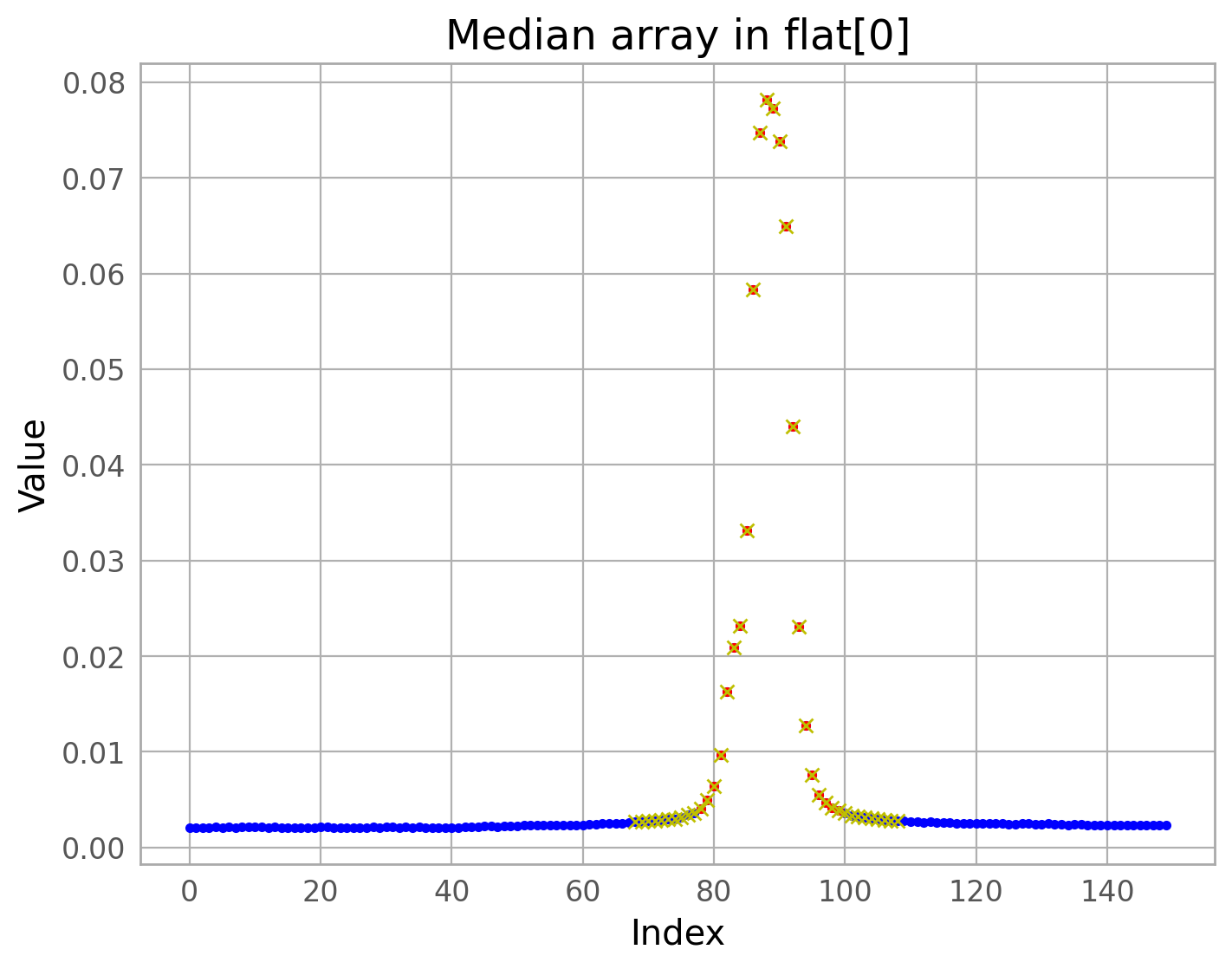
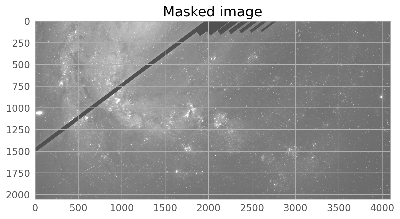
mask_satdet = make_mask(flc_file, 4, trail_segment, plot=True, verbose=True)
Rotation: -36.54276379722856
No good profile found for counter=20. Start moving left from starting point.
z=[] is less than 1, subr shape=(150, 200), we are done
Run time: 2.796928644180298 s

3.3 Running AstroDrizzle #
The next step is to run AstroDrizzle to combine the flc files into a final image, but first, we need to update the DQ array in the input fits file that contained the satellite trail. Once this information is in the DQ array, AstroDrizzle knows to ignore the flagged pixels when making the combined image. Below is one possible command to update the DQ array with one of the masks we created above using the update_dq, which sets the flagged pixels to 16384 in the DQ array. By default, we use the mask generated by findsat_mrt, but this can be changed. Note that if using the mask created by findsat_mrt, which was generated on a binned image, update_dq will automatically expand it to the original image dimensions.
Here, we are updating pixels in the DQ array of SCI,2 (extension 6). If we were flagging a satellite on the bottom chip (SCI,1 or extension 1), the update_dq function would instead be used to modify extension 3. More detail on the ACS file structure may be found in the ACS Data Handbook.
final_mask = mask_mrt  # uncomment this line to use the mask from findsat_mrt
# final_mask = mask_satdet  # uncomment this line to use the mask from satdet

update_dq(flc_file, 6, final_mask, verbose=True, expand_mask=True)

# note: if running findsat_mrt, you could also update the DQ array with:
# w.updatedq()
INFO:utils_findsat_mrt:Inconsistent mask sizes:
Input mask: (1025, 2048)
DQ array: (2051, 4096)
INFO:utils_findsat_mrt:Enlarging mask to original size.
INFO:utils_findsat_mrt:Duplicating end rows to match orig size
DQ flag value is 16384
Input... flagged NPIX=186248
Existing flagged NPIX=0
Newly... flagged NPIX=186248
id8m11g4q_flc.fits[6] updated
With the satellite masked, the images can be drizzled again. For brevity, only the top chip (SCI,2) of the image stack will be drizzled together to make a combined product. This is controlled in AstroDrizzle via the group parameter. In case you did not run the ACS example, you also need to define some environment variables.
# Set the locations of reference files to your local computer.
os.environ['CRDS_SERVER_URL'] = 'https://hst-crds.stsci.edu'
os.environ['CRDS_SERVER'] = 'https://hst-crds.stsci.edu'
os.environ['CRDS_PATH'] = './crds_cache'
os.environ['iref'] = './crds_cache/references/hst/wfc3/'
os.environ['jref'] = './crds_cache/references/hst/acs/'
# The following lines of code find and download the MDRIZTAB reference file.
input_images = sorted(glob.glob('i*_flc.fits'))

mdz = fits.getval(input_images[0], 'MDRIZTAB', ext=0).split('$')[1]
print('Searching for the MDRIZTAB file:', mdz)
!crds sync --hst --files {mdz} --output-dir {os.environ['iref']}
Searching for the MDRIZTAB file: 2ck18260i_mdz.fits
CRDS - INFO -  Symbolic context 'hst-latest' resolves to 'hst_1297.pmap'
CRDS - INFO -  Reorganizing 0 references from 'instrument' to 'flat'
CRDS - INFO -  Reorganizing from 'instrument' to 'flat' cache,  removing instrument directories.
CRDS - INFO -  Syncing explicitly listed files.
CRDS - INFO -  0 errors
CRDS - INFO -  0 warnings
CRDS - INFO -  4 infos
input_uvis_images = sorted(glob.glob('i*_flc.fits'))


def get_vals_from_mdriztab(input_uvis_images, kw_list=['driz_sep_bits',
                                                       'combine_type',
                                                       'driz_cr_snr',
                                                       'driz_cr_scale',
                                                       'final_bits']):

    '''Get only selected parameters from. the MDRIZTAB'''
    mdriz_dict = getMdriztabPars(input_uvis_images)

    requested_params = {}

    print('Outputting the following parameters:')
    for k in kw_list:
        requested_params[k] = mdriz_dict[k]
        print(k, mdriz_dict[k])

    return requested_params
selected_params = get_vals_from_mdriztab(input_uvis_images)
- MDRIZTAB: AstroDrizzle parameters read from row 2.
Outputting the following parameters:
driz_sep_bits 336
combine_type minmed
driz_cr_snr 3.5 3.0
driz_cr_scale 1.5 1.2
final_bits 336
We can now run the drizzling step and show the output
# To override any of the above values
# selected_params['final_bits']    = '64, 32'    #to treat saturated pixels 256 as bad and fill with NaN
# selected_params['driz_cr_snr']   = '4.0 3.5'   #less aggressive cr-rejection threshold

adriz(input_uvis_images,
      output='automatic_uvis',
      group='4',
      preserve=False,
      clean=True,
      build=False,
      context=False,
      skymethod='match',
      **selected_params)

clear_output()
# Display the combined science and weight images

sci = fits.getdata('automatic_uvis_drc_sci.fits')
wht = fits.getdata('automatic_uvis_drc_wht.fits')

fig = plt.figure(figsize=(15, 15))
ax1 = fig.add_subplot(2, 1, 1)
ax2 = fig.add_subplot(2, 1, 2)

ax1.imshow(sci, vmin=0.1, vmax=0.5, cmap='Greys_r', origin='lower')
ax1.set_xlabel('X')
ax1.set_ylabel('Y')
ax1.set_title('Drizzled science image')
ax2.imshow(wht, vmin=0, vmax=1000, cmap='Greys_r', origin='lower')
ax2.set_xlabel('X')
ax2.set_ylabel('Y')
ax2.set_title('Drizzled weight image')
Text(0.5, 1.0, 'Drizzled weight image')
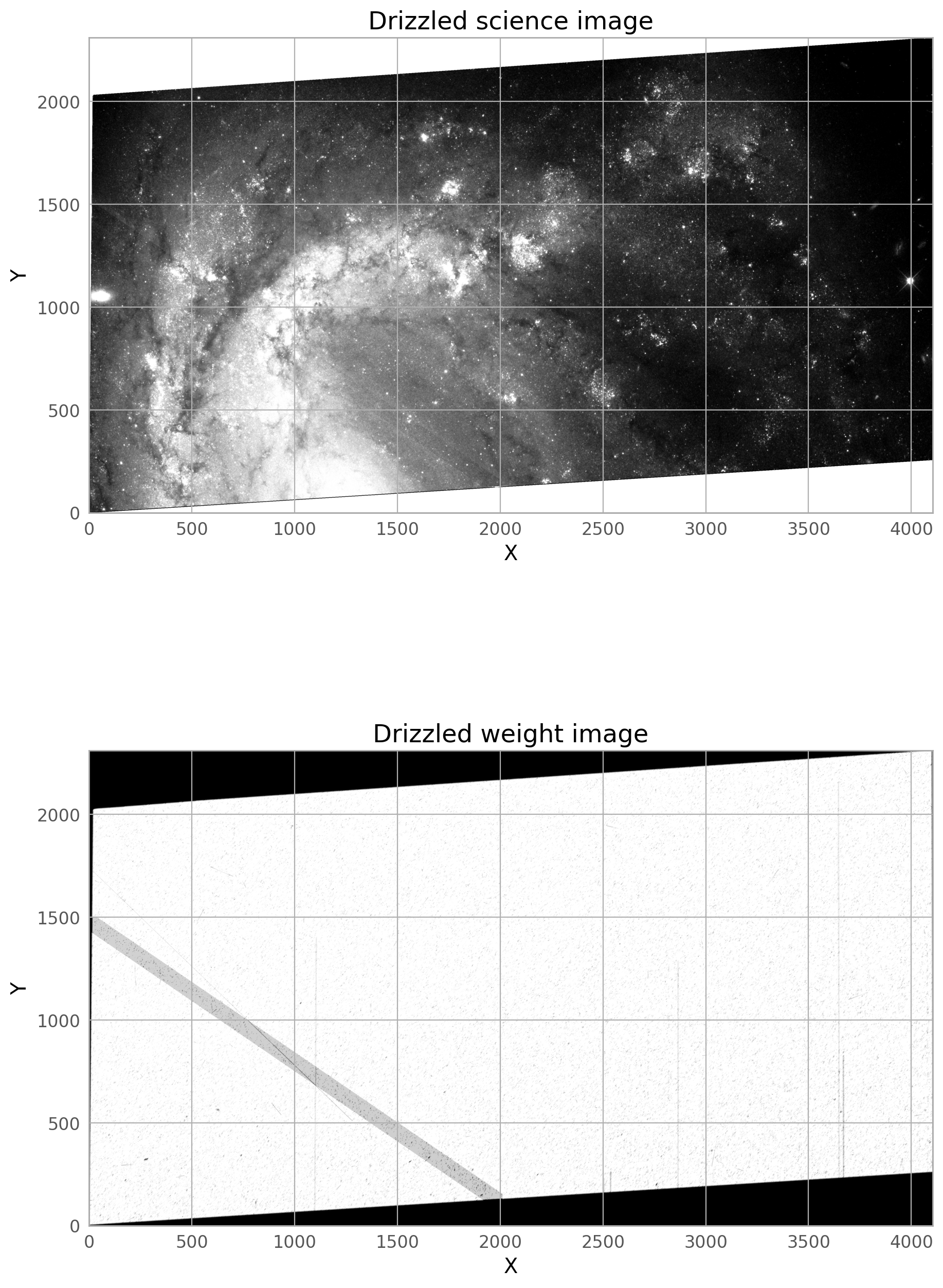
The final drizzled product shows that the bright satellite trail and its wings have been removed. If you don’t see the full trail removed, you may need to dilate the trail further, and make sure only the original i*_flc.fits images are getting incorporated into the drizzled image (if you are rerunning AstroDrizzle and are not careful with the inputs, files from previous runs could be used by accident).
About this Notebook #
Created: 14 Dec 2018; R. Avila
Updated: 12 Jun 2023; A. O'Connor
Updated: 12 Mar 2024; D. Stark
Updated: 15 May 2024; D. Stark, R. Avila, & J. Mack
Updated: 01 Oct 2025: M. Revalski, D. Stark
Source: GitHub spacetelescope/hst_notebooks
Additional Resources #
Below are some additional resources that may be helpful. Please send any questions through the HST Help Desk, selecting the DrizzlePac category.
Citations #
If you use public Python packages (e.g., astropy, astroquery, drizzlepac, matplotlib) for published research, please cite the authors. Follow these links for more information about citing various packages.
