Running the COS Data Pipeline (CalCOS)

Learning Goals:

This Notebook is designed to walk the user (you) through:

1. Setting up the Environment to Run CalCOS

- 1.1. Prerequisites

- 1.2. Create Your conda Environment

- 1.3. Imports and Basic Directories

- 1.4. Setup a Reference File directory

2. Gathering the Data to Run CalCOS

- 2.1. Downloading the Raw Data

- 2.2. Gathering Reference Files

3. Processing Raw COS data using CalCOS

- 3.1. Running CalCOS: From a Python Environment

- 3.2. Running CalCOS: From the Command Line

4. Re-processing COS Data with Altered Parameters

- 4.1. Altering the Calibration Switches

- 4.2. Running CalCOS with a Specific Set of Switches

- 4.3. Running CalCOS with a Different Reference File

This notebook currently fails to execute, use as reference only

0. Introduction

The Cosmic Origins Spectrograph (COS) is an ultraviolet spectrograph on-board the Hubble Space Telescope (HST) with capabilities in the near ultraviolet (NUV) and far ultraviolet (FUV).

CalCOS is the data processing pipeline which converts the raw data produced by COS’s detectors onboard HST into usable spectral data. It transforms the data from a list of many individual recorded photon interactions into tables of wavelength and flux.

This tutorial aims to prepare you run the CalCOS pipeline to reduce spectral data taken with the COS instrument. It focuses on COS data taken in TIME-TAG mode. Note that there is another, less commonly used mode, ACCUM, which should generally be used only for UV bright targets.

• For an in-depth manual to working with COS data and a discussion of caveats and user tips, see the COS Data Handbook.

• For a detailed overview of the COS instrument, see the COS Instrument Handbook.

Notes for those new to Python/Jupyter/Coding:

• You will frequently see exclamation points (!) or dollar signs ($) at the beginning of a line of code. These are not part of the actual commands. The exclamation points tell a Jupyter Notebook cell to pass the following line to the command line, and the dollar sign merely indicates the start of a terminal prompt.

1. Setting up the Environment to Run CalCOS

The first step to processing your data is setting up an environment from which to run CalCOS.

1.1. Prerequisites

This tutorial assumes some basic knowledge of the command line and was built using a unix style shell. Those using a Windows computer will likely have the best results if working within the Windows Subsystem for Linux.

If you do not already have any distribution of the conda tool, see this page for instructions, and install either anaconda (~ 3 GB, more beginner friendly, lots of extras you likely won’t use), miniconda (~ 400 MB, only what you need to make environments), or mamba (~85 MB, similar to miniconda but rewritten in C++).

1.2. Create Your conda Environment

Once you have conda installed, you can create an environment.

Open up your terminal app, likely Terminal or iTerm on a Mac or Windows Terminal or Powershell on Windows.

First, add the conda-forge channel to your computer’s conda channel list. This enables conda to look in the right place to find all the packages we want to install.

$ conda config --add channels conda-forge

Now we can create a new environment for running CalCOS; let’s call it calcos_env, and initialize it with Python version 3.10 and several packages we’ll need.

$ conda create -n calcos_env python=3.10 notebook jupyterlab numpy astropy matplotlib astroquery

After allowing conda to proceed to installing the packages (type y then hit enter), you can see all of your environments with:

$ conda env list

and then switch over to your new environment with:

$ conda activate calcos_env

Finally you must install the CalCOS and CRDS packages using pip:

$ pip install calcos crds

At this point, typing calcos --version into the command line and hitting enter should no longer yield the error:

command not found: calcos

but rather respond with a version number, i.e. version 3.4.4 at the time of writing this Notebook.

At this point, if you started this Jupyter Notebook in another Python environment, you should now quit that instance, run $ conda activate calcos_env, and reopen this Jupyter Notebook. If you’re unsure whether you’re already using the calcos_env environment, you can see the active environment with the following cell:

# Displays name of current conda environment
from os import environ, system
if "CONDA_DEFAULT_ENV" in environ:
    print("You are using:", environ["CONDA_DEFAULT_ENV"])
else:
    system("conda info --envs")

1.3. Imports and Basic Directories

We will import the following packages:

• calcos to run the COS data pipeline

• astroquery.mast Mast and Observations for finding and downloading data from the MAST archive

• numpy to handle array functions (version \(\ge\) 1.17)

• astropy.io fits for accessing FITS files

• astropy.table Table for creating and reading organized tables of the data

• matplotlib.pyplot for plotting data

• glob, shutil, and os for searching and working with system files and variables

• pathlib Path for managing system paths

import calcos
import numpy as np
from astropy.io import fits
from astropy.table import Table
import matplotlib.pyplot as plt
from astroquery.mast import Observations
import glob
import os
import shutil
from pathlib import Path

# This line makes plots appear in the Notebook instead of a separate window
%matplotlib inline

We will also define a few basic directories in which to place our inputs and outputs.

# These will be important directories for the Notebook
datadir = Path('./data/')
outputdir = Path('./output/')

# Make the directories if they don't exist
datadir.mkdir(exist_ok=True)
outputdir.mkdir(exist_ok=True)

1.4. Set up a Reference File Directory

CalCOS needs to be able to find all your reference files, (flat field image, bad pixel table, etc.), and the best way to enable that is to create a central directory of all the calibration files you’ll need. We refer to this directory as lref by convention, and set a system variable lref to the location of the directory. In this section, we will create the lref environment variable; however, we need to populate the lref folder with the actual reference files. We do this in Section 2.2. If you have already downloaded the set of COS reference files you need to use into an existing lref directory, you should instead set lref to the path to this directory.

We can assign a system variable in three different ways, depending on whether we are working from:

1. The command line

2. A Python environment

3. A Jupyter Notebook

Unix-style Command Line	Python	Jupyter Notebook
export lref=’./data/reference/…’	os.environ[“lref”] = “./data/reference/…”	%env lref ./data/reference/…

Note that this system variable must be set again with every new instance of a terminal - if you frequently need to use the same lref directory, consider adding an export statement to your .bash_profile or equivalent file.

Because this is a Jupyter Notebook, we set our reference directory with the cell magic below:

%env lref ./data/reference/references/hst/cos/

We can note the value of the system variable using the following command:

os.getenv('lref')

---

2. Gathering the Data to Run CalCOS

The CalCOS pipeline can be run either from a Python environment, or directly from a Unix-style command line. The two use the same underlying machinery but can differ in syntax. For specifics on the keywords to run CalCOS with specific behaviors and arguments, see Table 3.2: Arguments for Running CalCOS in Python and Table 3.3: Command-line Options for Running CalCOS in Unix/Linux/Mac.

2.1. Downloading the Raw Data

First, we need to make sure we have all of our data ready and in the right spot. If you are unfamiliar with searching the archive for data, we recommend that you view our tutorial on downloading COS data. This Notebook will largely gloss over downloading the data.

To run CalCOS, we will need the following files:

1. All the raw data from separate exposures we wish to combine as _rawtag FITS files

2. The association file telling CalCOS which files to combine as a _asn FITS file.

Note that we do not generally run the CalCOS pipeline directly on the data files, but instead on an association _asn file. This allows for the calibration of related exposures into combined _x1dsum files.

If you instead use _rawtag or _corrtag exposure files as your inputs, you will only receive the exposure-specific _x1d files as your outputs.

For this example, we’re choosing the dataset LCXV13040 of COS/FUV observing the quasar 3C48. In the cell below we download the data from the archive:

# Query the MAST archive for data with observation id starting with lcxv1304
q1 = Observations.query_criteria(
                        obs_id='lcxv1304*')

# Make a list of all products we could download with this file
pl = Observations.get_product_list(q1)

# Filter to a list of only the products which are association files (asn)
asn_file_list = pl[pl["productSubGroupDescription"] == 'ASN']

# Filter to a list of only therawtag files for both segments
rawtag_list = pl[
    (pl["productSubGroupDescription"] == 'RAWTAG_A') |
    (pl["productSubGroupDescription"] == 'RAWTAG_B')
]

# Download the rawtag and asn lists to the data directory
rawtag_locs = Observations.download_products(
                                rawtag_list,
                                download_dir=str(datadir))

asn_locs = Observations.download_products(
                                asn_file_list,
                                download_dir=str(datadir))

By default, each exposure’s files are downloaded to separate directories, as is the association file.

We need to move around these files to all be in the same directory, which we do below.

for lpath in rawtag_locs['Local Path']:
    Path(lpath).replace(datadir/os.path.basename(lpath))

for lpath in asn_locs['Local Path']:
    Path(lpath).replace(datadir/os.path.basename(lpath))
    asn_name = os.path.basename(lpath)

# Delete the now-empty nested subdirectories (./data/mastDownload)
shutil.rmtree(datadir/'mastDownload')

2.2. Gathering Reference Files

The following process of gathering reference files is given a detailed explanation in Section 3 of our Notebook on setting up an environment to work with COS data. Your process will be somewhat simpler and quicker if you have already downloaded the reference files.

Each data file has an associated set of calibration files which are needed to run the associated correction with (i.e. you need the FLATFILE to flat field correct the data). These reference files must be located in the $lref directory to run the pipeline.

The STScI team is regularly producing new calibration files in an effort to keep improving data reduction. Periodically the pipeline is re-run on all COS data. To determine which reference files were used most recently by STScI to calibrate your data, you can refer to your data file’s CRDS_CTX keyword in its FITS header:

# Find all of the raw files:
rawfiles = glob.glob(str(datadir/'*raw*.fits'))

# Get the header of the 0th raw file, look for its CRDS context keyword:
crds_ctx = fits.getheader(rawfiles[0])['CRDS_CTX']

# Print the file's CRDS context keyword:
print(f"The CRDS Context last run with {rawfiles[0]} was:\t{crds_ctx}")

The value of this keyword in the header is a .pmap or observatory context file which tells the CRDS calibration data distribution program which files to distribute. You can also find the newest “operational” context on the HST CRDS website.

To download the reference files specified by a context file, we use the crds tool we installed earlier.

---

If you haven’t already downloaded up-to-date reference files, (as in Section 3 of Setup Notebook, click to skip this cell and begin downloading the files!

If you have recently downloaded COS reference files, (i.e. if you ran Section 3 of the Setup Notebook,) you likely do not have to download more reference files. Instead, follow the instructions in this cell and then skip to Section 3.

If you already downloaded the files, you can simply point the pipeline to the ones you downloaded, using the crds bestrefs command, as shown in the following three steps. Run these steps from your command line if you already have the reference files in a local cache. Note also that there may be newer reference files available. To make sure you are always using the most up-to-date reference files, we advise you familiarize yourself with the newest files and documentation at the CRDS homepage.

1. The following sets the environment variable for crds to look for the reference data online:

$ export CRDS_SERVER_URL=https://hst-crds.stsci.edu

2. The following tells crds where to save the files it downloads - set this to the directory where you saved the crds_cache, i.e. in Section 3 of our Notebook on Setup:

$ export CRDS_PATH=${HOME}/crds_cache

3. The following will update the data files you downloaded so that they will be processed with the reference files you previously downloaded:

$ crds bestrefs --files data/*raw*.fits --update-bestrefs --new-context '<the imap or pmap file you used to download the reference files>'

Assuming everything ran successfully, you can now skip to Section 3.

---

If you have not yet downloaded the reference files, you will need to do so, as shown below:

Caution!

Note that as of the time of this Notebook’s update, the pipeline context used below was hst_1071.pmap, but this changes over time. You are running this in the future, and there is certainly a newer context you would be better off working with. Take a minute to consider this, and check the HST Calibration Reference Data System webpage to determine what the current operational pmap file is.

Unless we are connected to the STScI network, or already have the reference files on our machine, we will need to download the reference files and tell the pipeline where to look for the flat files, bad-pixel files, etc.

The process in the following two cells can take a long time and strain network resources. If you have already downloaded up-to-date COS reference files, we recommend that you avoid doing so again. Instead, keep these crds files in an accessible location, and point an environment variable lref to this directory. For instance, if your lref files are on your home directory in a subdirectory called crds_cache, give Jupyter the following command:

%env lref /Users/<your username>/crds_cache/references/hst/cos/

If you have an older cache of reference files, you may also simply update your cached reference files. Please see the CRDS Guide for more information.

Assuming you have not yet downloaded these files, in the next two cells, we will setup an environment of reference files, download the files, and save the output of the crds download process in a log file:

%%capture cap --no-stderr
# ^ The above puts the cell's output into a text file made in the next cell
# ^^ This avoids a very long printed output

# This sets an env variable for crds to look for the reference data online
%env CRDS_SERVER_URL https://hst-crds.stsci.edu

# This tells crds where to save the files it downloads
%env CRDS_PATH ./data/reference/

# This command looks up the pmap file, which tells what ref files to download.
# It then downloads these to the CRDS_PATH directory.
# Make sure you have the latest pmap file, found on the CRDS site.
!crds bestrefs --files data/*raw*.fits --sync-references=2
!crds bestrefs --update-bestrefs --new-context 'hst_1140.pmap'

We continue on to creating the CRDS output text file:

# This file will contain the output of the last cell
with open(outputdir / 'crds_output_1.txt', 'w') as f:
    f.write(cap.stdout)

We’ll print the beginning and end of crds_output_1.txt just to take a look.

# Creating a dictionary to store each line as a key & line info as a value
crds_output_dict = {}

# Open the file
with open(str(outputdir/'crds_output_1.txt'), 'r') as cell_outputs:
    # Loop through the lines in the text file
    for linenum, line in enumerate(cell_outputs):
        # Save each line to the defined dictionary
        crds_output_dict[linenum] = line[:-1]

# Get the length of the dictionary, aka, how many lines of output
total_lines = len(crds_output_dict)

print("Printing the first and last 5 lines of " + str(total_lines) +
      " lines output by the previous cell:\n")

for i in np.append(range(5), np.subtract(total_lines - 1, range(5)[::-1])):
    print(f"Line {i}:   \t", crds_output_dict[i])

# Delete the contents of the dict to avoid 'garbage' filling memory
crds_output_dict.clear()

Line 172 of the output should show 0 errors.

If you receive errors, you may need to attempt to run the crds bestrefs line again. These errors can arise from imperfect network connections.

It is recommended that you use this new $lref folder of reference files for subsequent CalCOS use, rather than re-downloading the reference files each time. To do this (after completing this Notebook):

• Save this folder somewhere accessibile, i.e. ~/crds_cache

• Add a line to your .bashrc or similar: export lref=<Path to your reference file directory>

  • If you wish to avoid adding this to your .bashrc, simply type the line above into any terminal you wish to run CalCOS from

  • If running CalCOS from a Jupyter Notebook, instead add a cell with: %env lref /Users/<Your Username>/crds_cache/references/hst/cos

3. Processing Raw COS Data Using CalCOS

Now we have all the reference files we need to run the CalCOS pipeline on our data.

This following cells which run the pipeline can take a while, sometimes more than 10 minutes!

By default, the pipeline also outputs hundreds of lines of text - we will suppress the printing of this text and instead save it to a text file.

3.1. Running CalCOS: From a Python Environment

Now, we can run the pipeline program:

Note that generally, CalCOS should be run on an association (_asn) file (check out the Notebook we have for creating or editing association files if you wish to alter the asn file that we downloaded). In this case, our association file is: ./data/lcxv13040_asn.fits. You may run CalCOS directly on _rawtag or _corrtag exposure files, but this will not produce an _x1dsum file and can result in errors for data taken at certain lifetime positions. No matter what type of files you run CalCOS on, you should only specify the FUVA segment’s file, i.e. the _rawtag_a file. If a rawtag_b file is in the same directory, CalCOS will find both segments’ files.

In this example, we also specify that verbosity = 2, resulting in a very verbose output, and we specify a directory to put all the output files in: output/calcos_processed_1. To avoid polluting this Notebook with more than a thousand lines of the output, we again capture the output of the next cell and save it to output/output_calcos_1.txt in the cell below.

%%capture cap --no-stderr
# Above ^ again, capture the output and save it in the next cell
# 1st param specifies which asn file to run the pipeline on
try:
    calcos.calcos(str(datadir/asn_name),
                  # verbosity param
                  verbosity=2,
                  # Save all resulting files in this subdirectory in our outdir
                  outdir=str(outputdir/"calcos_processed_1"))
except RuntimeError as e:
    print('An error occured, ', e)

# This file now contains the output of the previous cell
with open(str(outputdir/'output_calcos_1.txt'), 'w') as f:
    f.write(cap.stdout)

Again, we’ll print the beginning and end of that file just to take a look and make sure CalCOS ran successfully.

# Pair each line with its line number, start at 0
calcos_output_dict = {}

# Open the file
with open(str(outputdir/'output_calcos_1.txt'), 'r') as cell_outputs:
    # Loop through each line in output_calcos_1.txt
    for linenum, line in enumerate(cell_outputs):
        # Save each line to the dictionary we defined above
        calcos_output_dict[linenum] = line[:-1]

# Get the length of the dictionary - how many lines of output
total_lines = len(calcos_output_dict)

print("Printing the first and last 5 lines of "
      f"{total_lines} lines output by the previous cell:\n")
for i in np.append(range(5), np.subtract(total_lines - 1, range(5)[::-1])):
    print(f"Line {i}:   \t", calcos_output_dict[i])

# Delete the contents of the dictionary to save memory space
calcos_output_dict.clear()

3.2. Running CalCOS: From the Command Line

The syntax for running CalCOS from the command line is very similar. Assuming your data files, lref directory, and reference files are all where you’ve told CalCOS to look, you can simply run:

calcos -o directory_to_save_outputs_in filename_asn.fits

or, if you want to save a very verbose output to a log file log.txt:

calcos -v -o directory_to_save_outputs_in filename_asn.fits > log.txt

To see the full list of commands, Table 3.2: Command-line Options for Running CalCOS in Unix/Linux/Mac, or run the following with the name of the association file:

!calcos <PATH_TO_ASN_FILE>

4. Re-processing COS Data with Altered Parameters

4.1. Altering the Calibration Switches

The way to alter how CalCOS runs - i.e. which calibrations it performs - is with the calibration switches contained in the FITS headers.

The switches (with the exception of “XTRACTALG”), can be set to the values in the following table:

Value:	“PERFORM”	“OMIT”	“N/A”
Meaning:	Performs the calibration step	Does not perform the calibration step	This step would not make sense for this file

XTRACTALG instead can be set to either “BOXCAR” or “TWOZONE”, to specify the spectral extraction algorithm to be used. For more information, see Section 3.2.1: “Overview of TWOZONE extraction” of the Data Handbook.

In the cell below, we get a full list of the switches by name. If you want to learn more about the calibration steps and switches, see Chapters 2 and 3 of the COS Data Handbook.

# Reads the header of the 0th rawfile
header = fits.getheader(rawfiles[0])
# The calibration switches are found in lines 82 - 109 of the header
calibswitches = header[82:109]
calibswitches

Let’s begin by switching off all the switches currently set to “PERFORM” to a new value of “OMIT”, in every rawfile:

# Set to True to see a bit more about what is going on here
verbose = False

# Find each rawfile, i is a counter variable for the files you loop through
for rawfile in rawfiles:
    if verbose:
        print(rawfile)

    # Read that rawfiles header
    header = fits.getheader(rawfile)

    # Find all calibration switches
    corrections = [key for key in list(header.keys()) if "CORR" in key]

    # Checking if the value of each switch is 'PERFORM', and changing to 'OMIT'
    for correction in corrections:
        if header[correction] == 'PERFORM':
            if verbose:
                print("switching\t", header[correction],
                      "\t", correction, "\tto OMIT")
            # Turn off all the calib switches
            fits.setval(rawfile, correction, value='OMIT', ext=0)

In this case, CalCOS realizes that all the switches are set to “OMIT”, and exits without doing anything.

# Run CalCOS with all calib switches OFF; allow text output this time
try:
    calcos.calcos(
        str(datadir/asn_name),
        verbosity=0,
        outdir=str(outputdir/"calcos_processed_2")
    )
except RuntimeError as e:
    print('An error occured, ', e)

4.2. Running CalCOS with a Specific Set of Switches

Now, let’s set a single switch to “PERFORM”, and just run a flat-field correction (“FLATCORR”) and a pulse-height filter correction (“PHACORR”). Set verbosity = 1 or 2 to learn more about how CalCOS is working.

verbose = False

# Find each rawfile, i is a counter variable for the files you loop through
for rawfile in rawfiles:
    if verbose:
        print(rawfile)
    # Change the header's keyword FLATCORR to the value PERFORM
    fits.setval(rawfile, "FLATCORR", value='PERFORM', ext=0)
    # Change the header's keyword PHACORR to the value PERFORM
    fits.setval(rawfile, "PHACORR", value='PERFORM', ext=0)

%%capture cap --no-stderr
# Above ^ again, capture the output and save it in the next cell
try:
    calcos.calcos(
        str(datadir/asn_name),
        verbosity=2,
        outdir=str(outputdir/"calcos_processed_3")
    )
except RuntimeError as e:
    print('An error occured, ', e)

# This file now contains the output of the last cell
with open(str(outputdir/'output_calcos_3.txt'), 'w') as f:
    f.write(cap.stdout)

4.3. Running CalCOS with a Different Reference File

You may wish to run CalCOS with a specific flat file, bad pixel table, or any other reference file. CalCOS offers the ability to do just this on a file-by-file basis, by changing the calibration reference file values in the header of your data.

As an example, we check which calibration files are selected for one of our rawtag files.

# Read 0th rawfile's header
header = fits.getheader(rawfiles[0])
# The 110th to 138th lines of the header are filled with these reference files
refFiles = header[110:138]
# Get just the keywords i.e. "FLATFILE" and "DEADTAB"
refFile_keys = list(refFiles[2:].keys())
refFiles

For this section, let’s download another Pulse Height Amplitude (\_pha) table file using the crds tool:

!crds sync --files u1t1616ll_pha.fits --output-dir $lref

Now we can use the FITS headers to set this new file as the _pha file. As a demonstration, let’s do this for only the raw data from segment FUVA of the FUV detector:

Note that we are still only performing two corrections, as all calibration switches aside from FLATCORR and PHACORR are set to OMIT.

# Find just the FUVA raw files
rawfiles_segA = glob.glob(str(datadir/'*rawtag_a*.fits'))

# Iterate through each FUVA rawtag file to update the FITS header's PHATAB
for rawfileA in rawfiles_segA:
    print(rawfileA)
    # Updating the header value
    with fits.open(rawfileA, mode='update') as hdulist:
        # Update the 0th header of that FUVA file
        hdr0 = hdulist[0].header
        # NOTE: you need the $lref if you put it with your other ref files
        hdr0["PHATAB"] = 'lref$u1t1616ll_pha.fits'

Finally, let’s run CalCOS with the new _pha file for only the FUVA data:

%%capture cap --no-stderr
try:
    calcos.calcos(
                str(datadir/asn_name),
                verbosity=2,
                outdir=str(outputdir/"calcos_processed_4")
                )
except RuntimeError as e:
    print('An error occured, ', e)

# This file now contains the output of the last cell
with open(str(outputdir/'output_calcos_4.txt'), 'w') as f:
    f.write(cap.stdout)

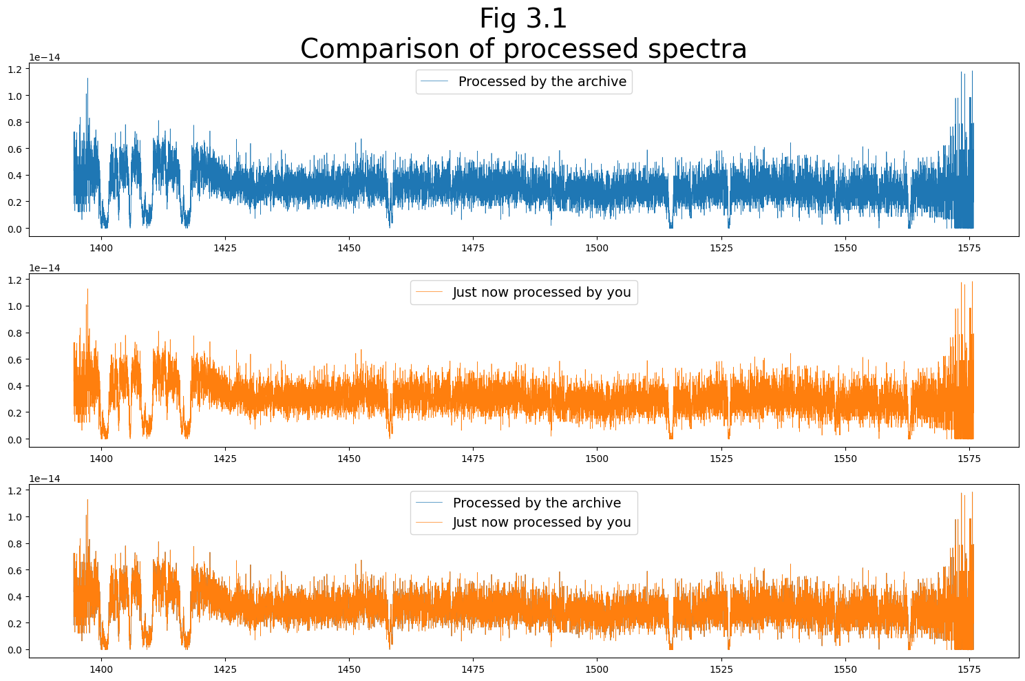
Before we go, let’s have a look at the spectra that we just calibrated and extracted

We’ll make a very quick plot to show the two spectra calibrated by STScI’s pipeline and by us right now. The two should agree very well. Small differences may be expected, given that the RANDSEED values may be different between the two versions.

Much more information on reading in and plotting COS spectra can be found in our other tutorial: Viewing COS Data.

(You can ignore the UnitsWarning below)

# Get the STScI calibrated x1dsum spectrum from the archive
Observations.download_products(Observations.get_product_list(
                                                Observations.query_criteria(
                                                        obs_id='lcxv13040')),
                               mrp_only=True,
                               download_dir='data/compare/'
                               )

# Read in this lcxv13040 spectrum
output_spectrum = Table.read(
    str(datadir/'compare/mastDownload/HST/lcxv13040/lcxv13040_x1dsum.fits'))

# Get the wavelength, flux, flux error, and data quality weight the X1DSUM file
# More info on the DQ_WGT can be found in Section 2.7 of the COS data handbook
wvln_orig = output_spectrum[1]["WAVELENGTH"]
flux_orig = output_spectrum[1]["FLUX"]
fluxErr_orig = output_spectrum[1]["ERROR"]
dqwgt_orig = output_spectrum[1]["DQ_WGT"]

# Convert the data quality (DQ) weight into a boolean to mask the data
dqwgt_orig = np.asarray(dqwgt_orig,
                        dtype=bool)

# Read in the spectrum we recently calibrated
output_spectrum = Table.read(
    str(outputdir/'calcos_processed_1/lcxv13040_x1dsum.fits'))

# Get the wavelength, flux, flux error, and data quality weight spectrum
new_wvln = output_spectrum[1]["WAVELENGTH"]
new_flux = output_spectrum[1]["FLUX"]
new_fluxErr = output_spectrum[1]["ERROR"]
new_dqwgt = output_spectrum[1]["DQ_WGT"]

# Convert the data quality weight into a boolean to mask the data
new_dqwgt = np.asarray(new_dqwgt,
                       dtype=bool)

# Build a 3 row x 1 column figure
fig, (ax0, ax1, ax2) = plt.subplots(3, 1, figsize=(15, 10))

# Plot the archive's spectrum in the top subplot
ax0.plot(wvln_orig[dqwgt_orig], flux_orig[dqwgt_orig],
         linewidth=0.5,
         c='C0',
         label="Processed by the archive")

# Plot your calibrated spectrum in the middle subplot
ax1.plot(new_wvln[new_dqwgt], new_flux[new_dqwgt],
         linewidth=0.5,
         c='C1',
         label="Just now processed by you")

# Plot the archived & newly calibrated spectra in bottom subplot
ax2.plot(wvln_orig[dqwgt_orig], flux_orig[dqwgt_orig],
         linewidth=0.5,
         c='C0',
         label="Processed by the archive")
ax2.plot(new_wvln[new_dqwgt], new_flux[new_dqwgt],
         linewidth=0.5,
         c='C1',
         label="Just now processed by you")

# Putting the legend on each subplot
ax0.legend(loc='upper center',
           fontsize=14)
ax1.legend(loc='upper center',
           fontsize=14)
ax2.legend(loc='upper center',
           fontsize=14)

# Setting the title of our plot
ax0.set_title("Fig 3.1\nComparison of processed spectra",
              size=28)

# Getting rid of the plot's whitespace
plt.tight_layout()

# Saving the figure to our output directory
# The 'dpi' parameter stands for 'dots per inch' (the res of the image)
plt.savefig(str(outputdir/"fig3.1_compare_plot.png"),
            dpi=300)

Congratulations! You finished this Notebook!

There are more COS data walkthrough Notebooks on different topics. You can find them here.

---

About this Notebook

Author: Nat Kerman - nkerman@stsci.edu

Updated On: 2023-03-30

This tutorial was generated to be in compliance with the STScI style guides and would like to cite the Jupyter guide in particular.

Citations

If you use astropy, matplotlib, astroquery, or numpy for published research, please cite the authors. Follow these links for more information about citations:

• Citing astropy

• Citing numpy

• Citing matplotlib

• Citing astroquery

---

Top of Page