
Evaluating STIS Target Acquisitions#
Table of Contents#
1. Introduction#
There are two types of STIS target acquisitions: ACQ and ACQ/PEAKUP. The ACQ is used in almost all STIS observations to center the target. The ACQ/PEAKUP can be taken after the ACQ to further refine the centering and is recommended for observations using slits with widths less than 0.2”. In this notebook, we will go through the steps for ACQ observations, and explore some success and failure cases.
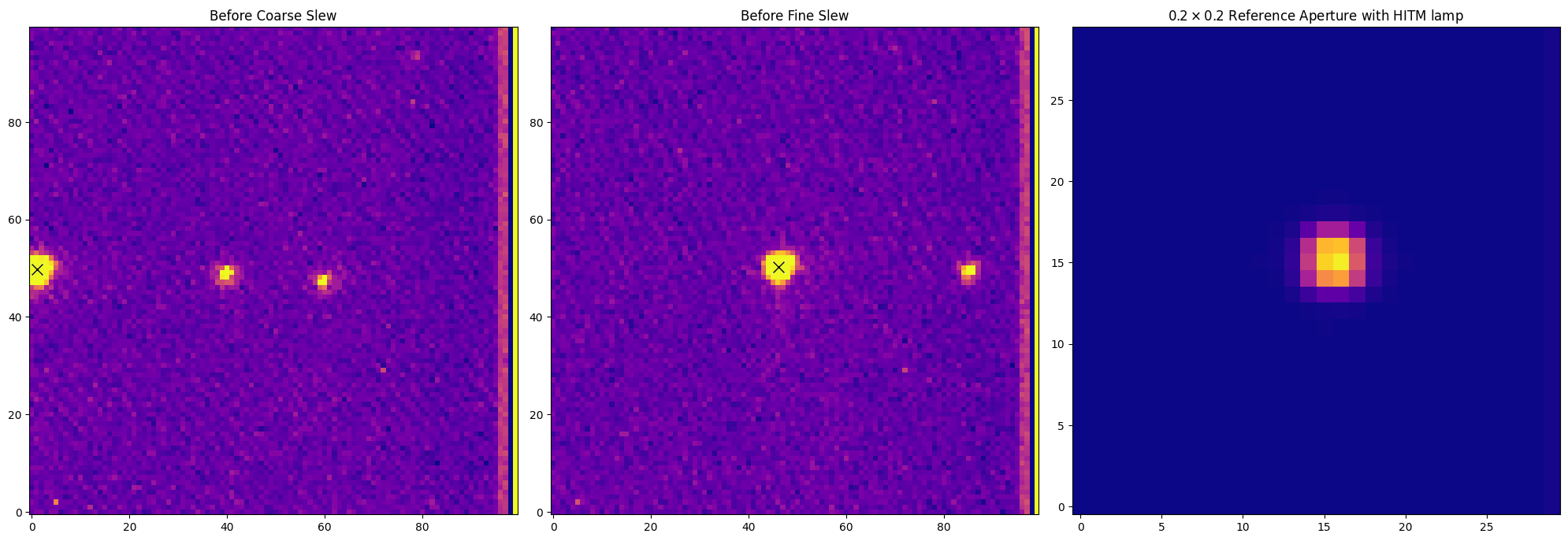
For ACQ observations, the target acquisition data has three science extensions:
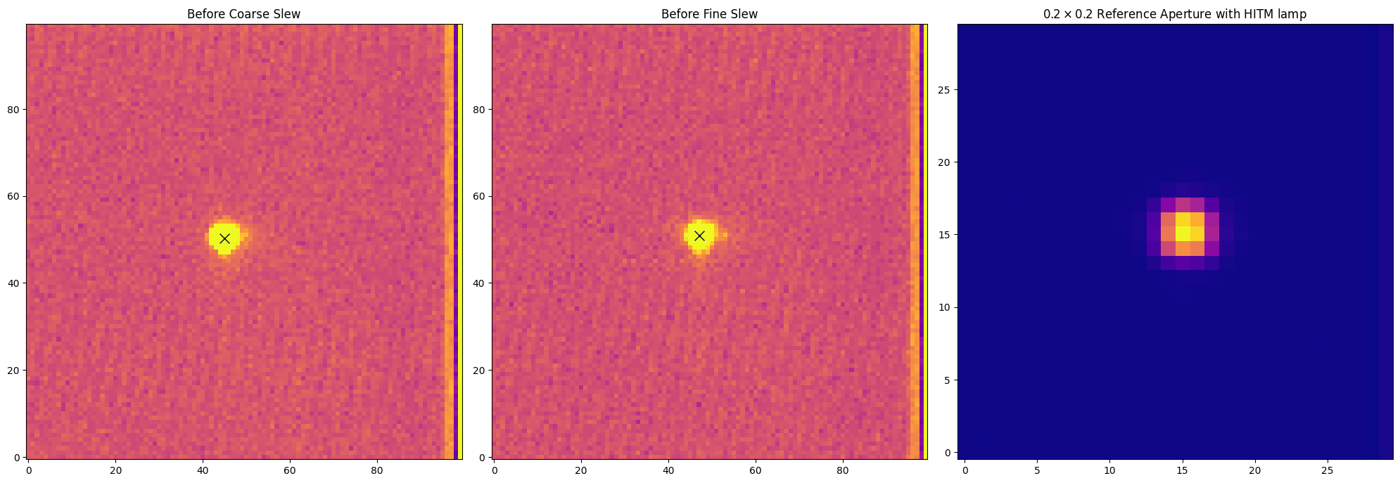
Before Coarse Slew
Before Fine Slew
0.2\(\times\)0.2 Reference Aperture with HITM lamp
The first science extension (Coarse Phase) of the acquisition raw file is an image of target in the target acquisition sub-array based on initial pointing. Then the coarse centering is performed: the software determines the position of the target with a flux weighted pointing algorithm, and calculates the slew needed to place the target at a reference point in the target acquisition sub-array; the coarse centered image is stored in the second science extension (Fine Phase). The next step is to perform fine centering: a 32 \(\times\) 32 pixel image of the reference aperture is obtained and stored in the third science extension (Reference Aperture), the location of the aperture on the detector is determined, and a fine slew is performed to center the taret in the reference aperture (to place the object precisely in a slit).
For more information on ACQ target acquisition, see Evaluating Target Acquisitions and Guiding.
1.1 Import necessary packages#
We will import the following packages:
astropy.io fitsfor accessing FITS filesastroquery.mast Observationsfor finding and downloading data from the MAST archiveosfor managing system pathsmatplotlibfor plotting datastistoolsfor quick operations on STIS Data
# Import for: Reading in fits file
from astropy.io import fits

# Import for: Downloading necessary files. (Not necessary if you choose to collect data from MAST)
from astroquery.mast import Observations

# Import for: Managing system variables and paths
import os

# Import for operations on STIS Data
import stistools

# Import for: Plotting and specifying plotting parameters
import matplotlib.pyplot as plt
import matplotlib
from astropy.visualization import ZScaleInterval
matplotlib.rcParams['image.origin'] = 'lower'
matplotlib.rcParams['image.cmap'] = 'plasma'
matplotlib.rcParams['image.interpolation'] = 'none'
matplotlib.rcParams['figure.figsize'] = (20, 7)
/home/runner/micromamba/envs/ci-env/lib/python3.11/site-packages/stsci/tools/nmpfit.py:8: UserWarning: NMPFIT is deprecated - stsci.tools v 3.5 is the last version to contain it.
  warnings.warn("NMPFIT is deprecated - stsci.tools v 3.5 is the last version to contain it.")
/home/runner/micromamba/envs/ci-env/lib/python3.11/site-packages/stsci/tools/gfit.py:18: UserWarning: GFIT is deprecated - stsci.tools v 3.4.12 is the last version to contain it.Use astropy.modeling instead.
  warnings.warn("GFIT is deprecated - stsci.tools v 3.4.12 is the last version to contain it."
The following tasks in the stistools package can be run with TEAL:
   basic2d      calstis     ocrreject     wavecal        x1d          x2d
2. Define Function for Plotting Acquisition Images and Performing Target Acquisition#
We define a function to plot the three science image extensions mentioned above, and run the stistools_tastis target acquisition method to show the result and associated information of target acquisition.
def acq(obs_id):
    # Search target object by obs_id
    target = Observations.query_criteria(obs_id=obs_id)
    # Get a list of files associated with that target
    acq_list = Observations.get_product_list(target)
    # Download only the _raw and _spt fits files
    Observations.download_products(acq_list, extension=['raw.fits', 'spt.fits'])
    raw = os.path.join("./mastDownload/HST", "{}".format(obs_id), "{}_raw.fits".format(obs_id))

    # Plot the acquisition raw images
    with fits.open(raw) as hdu:
        initial = hdu[1].data
        confirm = hdu[4].data
        lamp = hdu[7].data
    zscaler = ZScaleInterval(contrast=0.10).get_limits
    _, initial_max = zscaler(initial)
    _, confirm_max = zscaler(confirm)
    vmax = max(initial_max, confirm_max)

    # Plot the initial target position in coarse phase
    TARGA1_1 = fits.getheader(raw, 1)["TARGA1"]
    TARGA2_1 = fits.getheader(raw, 1)["TARGA2"]
    TARGA1_2 = fits.getheader(raw, 4)["TARGA1"]
    TARGA2_2 = fits.getheader(raw, 4)["TARGA2"]
    centera1 = fits.getheader(raw, 0)["CENTERA1"]
    centera2 = fits.getheader(raw, 0)["CENTERA2"]
    sizaxis1 = fits.getheader(raw, 0)["sizaxis1"]
    sizaxis2 = fits.getheader(raw, 0)["sizaxis2"]
    corner1 = centera1 - sizaxis1/2
    corner2 = centera2 - sizaxis2/2

    plt.subplot(1, 3, 1)
    plt.imshow(initial, vmin=0, vmax=vmax)
    plt.plot([TARGA1_1-corner1+1], [TARGA2_1-corner2+1], "x", c="white", markersize=12)
    plt.plot([TARGA1_1-corner1+1], [TARGA2_1-corner2+1], "x", c="black", markersize=10)
    plt.title("Before Coarse Slew")
    plt.subplot(1, 3, 2)
    plt.imshow(confirm, vmin=0, vmax=vmax)
    plt.plot([TARGA1_2-corner1+1], [TARGA2_2-corner2+1], "x", c="white", markersize=12)
    plt.plot([TARGA1_2-corner1+1], [TARGA2_2-corner2+1], "x", c="black", markersize=10)
    plt.title("Before Fine Slew")
    plt.subplot(1, 3, 3)
    plt.imshow(lamp, vmin=0, vmax=6000)
    plt.title(r"$0.2 \times 0.2$ Reference Aperture with HITM lamp")
    plt.tight_layout()

    stistools.tastis.tastis(raw)
The PDQ quality flags of the dataset are indicated in the “QUALITY” field of the raw fits file 0th header, and telemetry comments are saved in the “QUALCOM” fields of the 0th header. The same comments can also be seen on the Preview page of the dataset on the MAST archive. We can get those fields to confirm the potential reasons for acquisition failure:
def get_telemetry(obs_id):
    raw_file = "./mastDownload/HST/{id}/{id}_raw.fits".format(id=obs_id)
    quality = fits.getval(raw_file, "QUALITY", ext=0)
    QUALCOM1 = fits.getval(raw_file, "QUALCOM1", ext=0)
    QUALCOM2 = fits.getval(raw_file, "QUALCOM2", ext=0)
    QUALCOM3 = fits.getval(raw_file, "QUALCOM3", ext=0)
    print(f'The quality of this exposure is {quality}. {QUALCOM1} {QUALCOM2} {QUALCOM3}')
3. Successful Target Acquisition#
Here we present a successful target acquisition case in which the target is correctly selected from the initial pointing image, coarse centering and fine centering are successfully performed, and the target is eventually centered in the slit. The target location, coarse slew, and fine slew data are printed by stistools.tastis. Note here that the coordinate system of tastis is 1-indexed while Python is 0-indexed.
acq("octka2daq")
INFO: Found cached file ./mastDownload/HST/octka2daq/octka2daq_spt.fits with expected size 155520. [astroquery.query]
INFO: Found cached file ./mastDownload/HST/octka2daq/octka2daq_raw.fits with expected size 129600. [astroquery.query]
===============================================================================
octka2daq       HST/STIS    MIRVIS      F25ND3             ACQ/POINT
prop: 14161      visit: A2    line: 1   target: HD-84937
obs date, time: 2016-04-30    10:09:43   exposure time:  2.10
dom GS/FGS: N6U6000023F2    sub-dom GS/FGS: N6U7000178F1
ACQ params:     bias sub: 1510   checkbox: 3      method: FLUX CENTROID
subarray (axis1,axis2):   size=(100,100)          corner=(487,466)
-------------------------------------------------------------------------------
Coarse locate phase:           Target flux in max checkbox (Counts): 3194

                       global          local
                    axis1 axis2     axis1 axis2
Target location:    531.9  516.2    45.9  51.2

                    axis1 axis2     axis1  axis2         V2      V3
                      (pixels)        (arcsec)            (arcsec)
Estimated slew:     -3.8   0.2    -0.196  0.010       -0.131 -0.145
-------------------------------------------------------------------------------
Fine locate phase:            Target flux in max checkbox (Counts): 3194

                       global            local
                    axis1 axis2     axis1 axis2
Target location:    534.1  516.9    48.1  51.9
Ref ap location:    537.4  516.3    19.4  16.3

                    axis1 axis2     axis1  axis2         V2      V3
                      (pixels)        (arcsec)           (arcsec)
Estimated slew:     -2.1   0.6     -0.104  0.030      -0.052 -0.095
-------------------------------------------------------------------------------
Total est. slew:    -5.9   0.8    -0.300  0.041        -0.183 -0.241
-------------------------------------------------------------------------------
Your ACQ appears to have succeeded, as the fluxes in the coarse
and fine stages agree within 25% and the fine slews were less than
4 pixels as expected

===============================================================================
4. Target Acquisition Failure Cases#
The tastis analyzes STIS target acquisitions, and prints warning information if the acquisition fails. The possible tastis failures are:
Telemetry indicates that the intended exposures may not have been performed. Check the images for signal.
The fine slew (to center the target in the reference aperture) is larger than 4 pixels. This may indicate a problem with your acquisition.
The fluxes in the maximum checkbox in the fine and coarse stages differ by more than 25%. This may indicate a problem with your acquisition.
The flux in the third image of the ACQ is lower than the typical value for the lamp; the image should be checked to see if the lamp was illuminated.
Saturation of pixels in the second image may have affected the final centering.
Sometimes a failure case might be caused by multiple acquisition warnings. In this section, we will go through several typical cases of acquisition failure.
4.1 Guide Stars not Acquired#
The Take Data Flag (TDF) is an onboard pointing control system flag which, when ON, indicates that the spacecraft is ready for an observation and that the guide star tracking performance is nomial. If the TDF is down, exposures are not performed until TDF comes up.
If the guide stars are not acquired during acquisition, the TDF will be turned down and no exposures will be performed. Therefore all acquisition images will be dark.
In this failure case, as telemetry indicates, the TDF is down at the start and no exposure was performed. Thus there is not a clear bright source in the Before Coarse Slew and Before Fine Slew images. Usually, exposure failures can also cause other issues such as fine slew larger than 4 pixels or Ratio of Flux in Max Checkbox in Fine & Coarse Stages Greater than 25%, because the tastis algorithm cannot pick up the proper bright source in the image to perform the following steps of acquisition.
acq("oeds03rzq")
INFO: Found cached file ./mastDownload/HST/oeds03rzq/oeds03rzq_spt.fits with expected size 155520. [astroquery.query]
INFO: Found cached file ./mastDownload/HST/oeds03rzq/oeds03rzq_raw.fits with expected size 129600. [astroquery.query]
===============================================================================
oeds03rzq       HST/STIS    MIRVIS     F28X50LP             ACQ/POINT
prop: 16218      visit: 03    line: 1   target: 47TUC-OFFSET1
obs date, time: 2022-02-24    05:53:24   exposure time:  2.27
dom GS/FGS: S0W5000538F2    sub-dom GS/FGS: S0WC000284F1
ACQ params:     bias sub: 1536   checkbox: 3      method: FLUX CENTROID
subarray (axis1,axis2):   size=(100,100)          corner=(487,466)
-------------------------------------------------------------------------------
Coarse locate phase:           Target flux in max checkbox (Counts): 106

                       global          local
                    axis1 axis2     axis1 axis2
Target location:    533.0  564.0    47.0  99.0

                    axis1 axis2     axis1  axis2         V2      V3
                      (pixels)        (arcsec)            (arcsec)
Estimated slew:     -2.7  48.0    -0.139  2.438        1.626 -1.822
-------------------------------------------------------------------------------
Fine locate phase:            Target flux in max checkbox (Counts): 103

                       global            local
                    axis1 axis2     axis1 axis2
Target location:    536.0  563.0    50.0  98.0
Ref ap location:     1.0   1.0    -517.0  -499.0

                    axis1 axis2     axis1  axis2         V2      V3
                      (pixels)        (arcsec)           (arcsec)
Estimated slew:     536.3  562.0     27.242 28.550      39.451 -0.924
-------------------------------------------------------------------------------
Total est. slew:    533.5  610.0    27.104 30.988        41.077 -2.746
-------------------------------------------------------------------------------
Telemetry indicates that the intended exposures may not have
been performed.  Check the images for signal.

The fine slew (to center the target in the reference aperture) is larger
than 4 pixels.  This may indicate a problem with your acquisition.

The flux in the third image of the ACQ is lower than the typical value for
)the lamp; the image should be checked to see if the lamp was illuminated.

===============================================================================
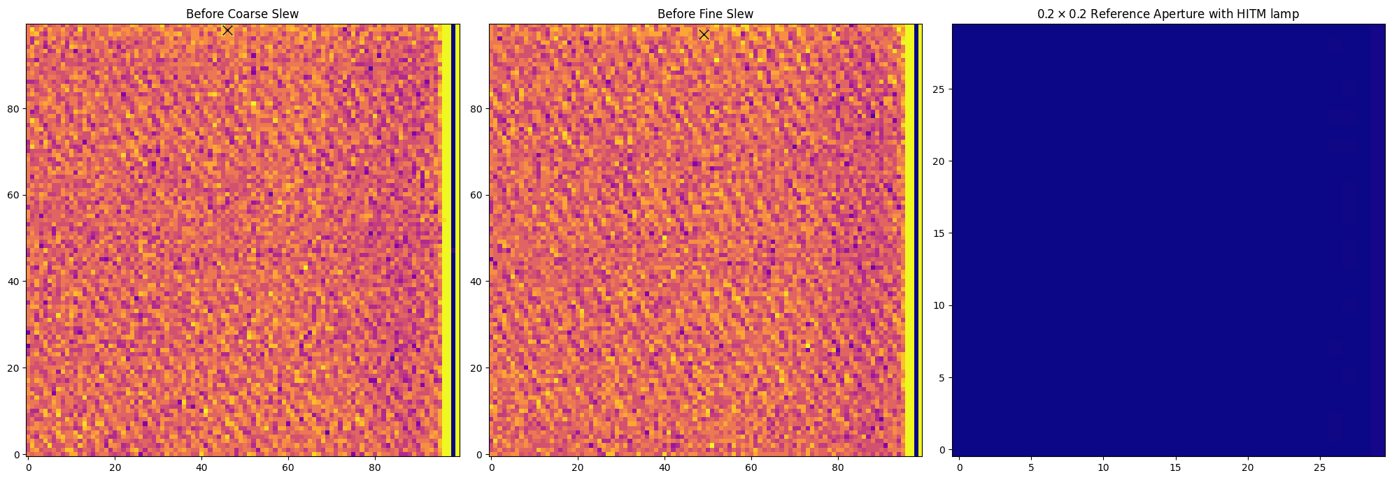
Telemetry of this observation confirms that the guide star acquisition failed and the aperture door was closed throughout the exposure:
get_telemetry("oeds03rzq")
The quality of this exposure is GSFAIL. Guide star acquisition failed. Observation taken on gyros only. STIS CCD aperture door shut throughout exposure.
4.2 Guide Star Acquisition Delayed#
In this failure case, the guide star acquisition is delayed during the coarse phase, but the guide stars are then acquired in the fine phase. Therefore the first acquisition image is dark while the target is in the second acquisition image. Eventually the target will still be centered, but the large fine slews may result in less precise positioning.
acq("oe1l55vjq")
INFO: Found cached file ./mastDownload/HST/oe1l55vjq/oe1l55vjq_spt.fits with expected size 155520. [astroquery.query]
INFO: Found cached file ./mastDownload/HST/oe1l55vjq/oe1l55vjq_raw.fits with expected size 129600. [astroquery.query]
===============================================================================
oe1l55vjq       HST/STIS    MIRVIS      F25ND5             ACQ/POINT
prop: 15905      visit: 55    line: 1   target: FOMALHAUT2
obs date, time: 2021-08-20    08:11:54   exposure time:  2.87
dom GS/FGS: SBKK000020F3    sub-dom GS/FGS: SBLC000216F2
ACQ params:     bias sub: 1536   checkbox: 3      method: FLUX CENTROID
subarray (axis1,axis2):   size=(100,100)          corner=(487,466)
-------------------------------------------------------------------------------
Coarse locate phase:           Target flux in max checkbox (Counts): 106

                       global          local
                    axis1 axis2     axis1 axis2
Target location:    541.0  516.9    55.0  51.9

                    axis1 axis2     axis1  axis2         V2      V3
                      (pixels)        (arcsec)            (arcsec)
Estimated slew:      5.3   0.9     0.267  0.046        0.221  0.156
-------------------------------------------------------------------------------
Fine locate phase:            Target flux in max checkbox (Counts): 21788

                       global            local
                    axis1 axis2     axis1 axis2
Target location:    538.0  513.9    52.0  48.9
Ref ap location:    536.6  516.3    18.6  16.3

                    axis1 axis2     axis1  axis2         V2      V3
                      (pixels)        (arcsec)           (arcsec)
Estimated slew:      2.6  -2.4      0.135 -0.122       0.009  0.181
-------------------------------------------------------------------------------
Total est. slew:     7.9  -1.5     0.401 -0.076         0.230  0.338
-------------------------------------------------------------------------------
Telemetry indicates that the intended exposures may not have
been performed.  Check the images for signal.

The fluxes in the maximum checkbox in the fine and coarse stages differ
by more than 25%.  This may indicate a problem with your acquisition.

===============================================================================
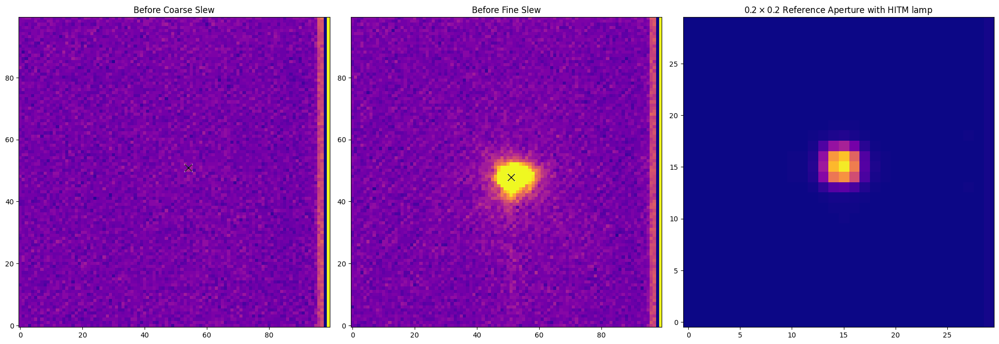
Telemetry of this observation suggests that the guide star acquisition was delayed and the exposure was shortened:
get_telemetry("oe1l55vjq")
The quality of this exposure is GSFAIL; EXPSHORT; TDF-DOWN. Guide star acquisition delayed. STIS CCD aperture door shut throughout exposure.
4.3 Lamp not illuminated#
As shown in the reference aperture, the reference aperture HITM lamp is dark and it has a flux smaller than the typical minumun value for the lamp. Usually, this kind of failure occurs if the TDF is down when the lamp image is taken; however, in some rare cases, the lamp might not be functioning. If the lamp image is blank, the target might not be centered in the reference aperture.
acq("oec62hj6q")
INFO: Found cached file ./mastDownload/HST/oec62hj6q/oec62hj6q_spt.fits with expected size 155520. [astroquery.query]
INFO: Found cached file ./mastDownload/HST/oec62hj6q/oec62hj6q_raw.fits with expected size 129600. [astroquery.query]
===============================================================================
oec62hj6q       HST/STIS    MIRVIS     F28X50LP             ACQ/POINT
prop: 16230      visit: 2H    line: 1   target: LMC-X-4
obs date, time: 2021-04-11    23:09:27   exposure time:  4.77
dom GS/FGS: S13H000373F1    sub-dom GS/FGS: S13H000845F2
ACQ params:     bias sub: 1536   checkbox: 3      method: FLUX CENTROID
subarray (axis1,axis2):   size=(100,100)          corner=(487,466)
-------------------------------------------------------------------------------
Coarse locate phase:           Target flux in max checkbox (Counts): 3788

                       global          local
                    axis1 axis2     axis1 axis2
Target location:    534.7  515.0    48.7  50.0

                    axis1 axis2     axis1  axis2         V2      V3
                      (pixels)        (arcsec)            (arcsec)
Estimated slew:     -1.0  -1.0    -0.052 -0.051       -0.073 -0.001
-------------------------------------------------------------------------------
Fine locate phase:            Target flux in max checkbox (Counts): 3955

                       global            local
                    axis1 axis2     axis1 axis2
Target location:    533.9  516.3    47.9  51.3
Ref ap location:     1.0   1.0    -517.0  -499.0

                    axis1 axis2     axis1  axis2         V2      V3
                      (pixels)        (arcsec)           (arcsec)
Estimated slew:     534.2  515.3     27.136 26.177      37.698  0.678
-------------------------------------------------------------------------------
Total est. slew:    533.1  514.3    27.084 26.126        37.625  0.677
-------------------------------------------------------------------------------
The fine slew (to center the target in the reference aperture) is larger
than 4 pixels.  This may indicate a problem with your acquisition.

The flux in the third image of the ACQ is lower than the typical value for
)the lamp; the image should be checked to see if the lamp was illuminated.

===============================================================================
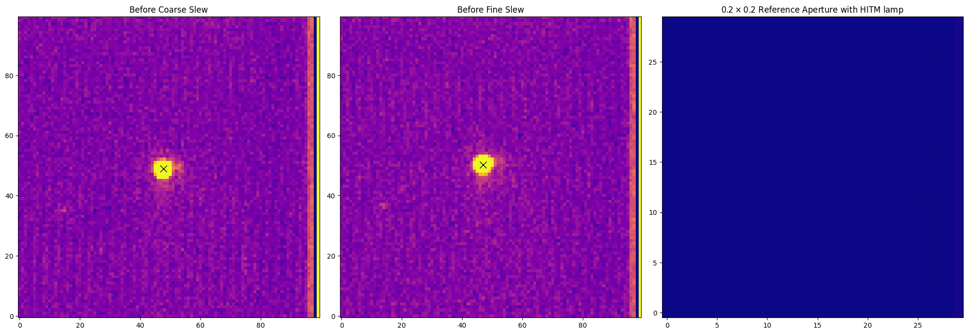
The LOCKLOST quality flag suggests that guide star was lost during the guide period, and thus the exposure was shortened and the lamp was not illuminated:
get_telemetry("oec62hj6q")
The quality of this exposure is EXPSHORT; LOCKLOST; TDF-DOWN. Take Data Flag NOT on throughout observation. STIS CCD shutter closed during all or part of exposure.
4.4 Multiple Bright Sources#
If there are multiple bright sources in a single acquisition image, the maximum checkbox will go through the image and find the brightest one. However, the presence of a source brighter than the target might confuse the algorithm and the acquisition might center at the wrong target.
acq("odkt01bvq")
INFO: Found cached file ./mastDownload/HST/odkt01bvq/odkt01bvq_spt.fits with expected size 155520. [astroquery.query]
INFO: Found cached file ./mastDownload/HST/odkt01bvq/odkt01bvq_raw.fits with expected size 129600. [astroquery.query]
===============================================================================
odkt01bvq       HST/STIS    MIRVIS     F28X50LP             ACQ/POINT
prop: 15273      visit: 01    line: 1   target: V838HER
obs date, time: 2018-10-01    06:13:32   exposure time: 50.10
dom GS/FGS: N28G000937F2    sub-dom GS/FGS: N28G000392F1
ACQ params:     bias sub: 1536   checkbox: 3      method: FLUX CENTROID
subarray (axis1,axis2):   size=(100,100)          corner=(487,466)
-------------------------------------------------------------------------------
Coarse locate phase:           Target flux in max checkbox (Counts): 1935

                       global          local
                    axis1 axis2     axis1 axis2
Target location:    488.1  515.8     2.1  50.8

                    axis1 axis2     axis1  axis2         V2      V3
                      (pixels)        (arcsec)            (arcsec)
Estimated slew:     -47.6  -0.2    -2.420 -0.010       -1.718 -1.704
-------------------------------------------------------------------------------
Fine locate phase:            Target flux in max checkbox (Counts): 1989

                       global            local
                    axis1 axis2     axis1 axis2
Target location:    533.2  516.2    47.2  51.2
Ref ap location:    537.6  516.3    19.6  16.3

                    axis1 axis2     axis1  axis2         V2      V3
                      (pixels)        (arcsec)           (arcsec)
Estimated slew:     -3.1  -0.1     -0.159 -0.005      -0.116 -0.109
-------------------------------------------------------------------------------
Total est. slew:    -50.8  -0.3    -2.579 -0.015        -1.834 -1.813
-------------------------------------------------------------------------------
Your ACQ appears to have succeeded, as the fluxes in the coarse
and fine stages agree within 25% and the fine slews were less than
4 pixels as expected

===============================================================================
4.5 Saturation of Pixels#
For the CCD detector, if a pixel is saturated, the excess charge will leak to adjacent pixels in the column. Saturations of pixels will affect the target flux in the max checkbox and the final centering.
acq("oe4h03rdq")
INFO: Found cached file ./mastDownload/HST/oe4h03rdq/oe4h03rdq_spt.fits with expected size 155520. [astroquery.query]
INFO: Found cached file ./mastDownload/HST/oe4h03rdq/oe4h03rdq_raw.fits with expected size 129600. [astroquery.query]
===============================================================================
oe4h03rdq       HST/STIS    MIRVIS     F28X50LP             ACQ/POINT
prop: 15836      visit: 03    line: 1   target: V-AU-MIC-1
obs date, time: 2020-07-03    00:20:25   exposure time:  0.50
dom GS/FGS: SCLW000169F1    sub-dom GS/FGS: SCLW000085F2
ACQ params:     bias sub: 1536   checkbox: 3      method: FLUX CENTROID
subarray (axis1,axis2):   size=(100,100)          corner=(487,466)
-------------------------------------------------------------------------------
Coarse locate phase:           Target flux in max checkbox (Counts): 233847

                       global          local
                    axis1 axis2     axis1 axis2
Target location:    534.8  513.0    48.8  48.0

                    axis1 axis2     axis1  axis2         V2      V3
                      (pixels)        (arcsec)            (arcsec)
Estimated slew:     -0.9  -3.0    -0.047 -0.152       -0.141  0.074
-------------------------------------------------------------------------------
Fine locate phase:            Target flux in max checkbox (Counts): 218485

                       global            local
                    axis1 axis2     axis1 axis2
Target location:    533.9  516.9    47.9  51.9
Ref ap location:    537.5  515.5    19.5  15.5

                    axis1 axis2     axis1  axis2         V2      V3
                      (pixels)        (arcsec)           (arcsec)
Estimated slew:     -2.3   1.4     -0.118  0.071      -0.033 -0.134
-------------------------------------------------------------------------------
Total est. slew:    -3.3  -1.6    -0.166 -0.081        -0.175 -0.060
-------------------------------------------------------------------------------
Saturation of pixels in the second image may have affected
the final centering.

===============================================================================
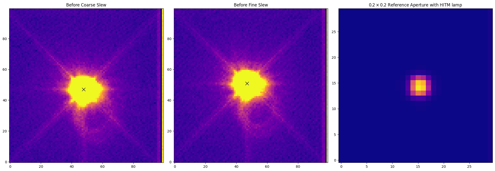
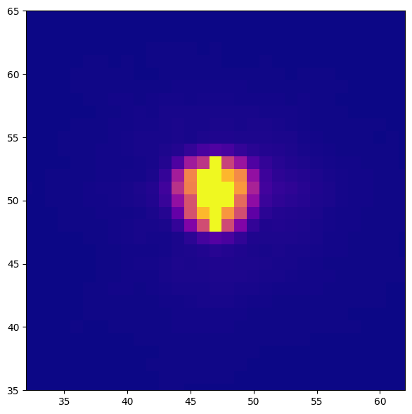
If we zoom in to the center of the second acquisition image and change the color scale, we can see that the pixels in the center are saturated, and the excess charges follow downward along the column so that the pixels below are affected.
raw = os.path.join("./mastDownload/HST", "{}".format("oe4h03rdq"), "{}_raw.fits".format("oe4h03rdq"))
with fits.open(raw) as hdu:
    confirm = hdu[4].data
plt.imshow(confirm, vmin=0, vmax=1e4)
plt.xlim(32, 62)
plt.ylim(35, 65)
(35.0, 65.0)
4.6 No Target in the Acquisition Image#
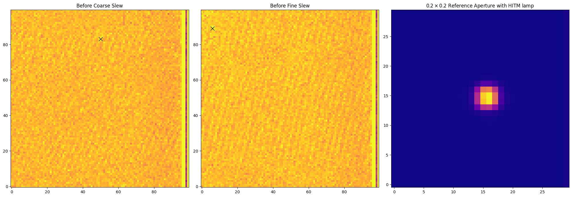
In this failure case, the guide stars were acquired successfully, and the TDF is always on through the exposure. However, the first and second acquisition images are blank and no target is acquired. This kind of failure happens if the submitted target location/orientation is wrong, or the source is too faint to be observed.
acq("ocyg39yoq")
INFO: Found cached file ./mastDownload/HST/ocyg39yoq/ocyg39yoq_spt.fits with expected size 155520. [astroquery.query]
INFO: Found cached file ./mastDownload/HST/ocyg39yoq/ocyg39yoq_raw.fits with expected size 129600. [astroquery.query]
===============================================================================
ocyg39yoq       HST/STIS    MIRVIS     F28X50LP             ACQ/POINT
prop: 14257      visit: 39    line: 1   target: C2013X1
obs date, time: 2016-06-10    12:33:13   exposure time:  2.10
dom GS/FGS: SCJV000223F1    sub-dom GS/FGS: NONE
ACQ params:     bias sub: 1510   checkbox: 3      method: FLUX CENTROID
subarray (axis1,axis2):   size=(100,100)          corner=(487,466)
-------------------------------------------------------------------------------
Coarse locate phase:           Target flux in max checkbox (Counts): 295

                       global          local
                    axis1 axis2     axis1 axis2
Target location:    537.0  549.0    51.0  84.0

                    axis1 axis2     axis1  axis2         V2      V3
                      (pixels)        (arcsec)            (arcsec)
Estimated slew:      1.3  33.0     0.065  1.676        1.231 -1.140
-------------------------------------------------------------------------------
Fine locate phase:            Target flux in max checkbox (Counts): 304

                       global            local
                    axis1 axis2     axis1 axis2
Target location:    493.0  555.0     7.0  90.0
Ref ap location:    537.5  515.5    19.5  15.5

                    axis1 axis2     axis1  axis2         V2      V3
                      (pixels)        (arcsec)           (arcsec)
Estimated slew:     -43.2  39.5     -2.196  2.007      -0.134 -2.972
-------------------------------------------------------------------------------
Total est. slew:    -42.0  72.5    -2.132  3.683         1.097 -4.112
-------------------------------------------------------------------------------
The fine slew (to center the target in the reference aperture) is larger
than 4 pixels.  This may indicate a problem with your acquisition.

===============================================================================
About this Notebook #
Author: Keyi Ding
Updated On: 2025-11-05
This tutorial was generated to be in compliance with the STScI style guides and would like to cite the Jupyter guide in particular.
Citations #
If you use astropy, matplotlib, astroquery, or numpy for published research, please cite the
authors. Follow these links for more information about citations:
