Modifying or Creating an Association File

Modifying or Creating an Association File#

Learning Goals#

This Notebook is designed to walk the user (you) through: Creating or altering the association (asn) file used by the Cosmic Origins Spectrograph (COS) pipeline to determine which data to process:

1. Examining an association file

2. Editing an existing association file

- 2.1. Removing an exposure

+ 2.1.1. Removing a bad exposure

+ 2.1.2. Filtering to a single exposure (e.g. for LP6 data)

- 2.2. Adding an exposure

3. Creating an entirely new association file

- 3.1. Simplest method

- 3.2. With FITS header metadata

- 3.3. Association files for non-TAGFLASH datasets

+ 3.3.1. Gathering the exposure information

+ 3.3.2. Creating the SPLIT wavecal association file

0. Introduction#

The Cosmic Origins Spectrograph (COS) is an ultraviolet spectrograph on-board the Hubble Space Telescope (HST) with capabilities in the near ultraviolet (NUV) and far ultraviolet (FUV).

This tutorial aims to prepare you to alter the association file used by the CalCOS pipeline. Association files are fits files containing a binary table extension, which list their “member” files: science and calibration exposures which the pipeline will process together into spectral data products.

For an in-depth manual to working with COS data and a discussion of caveats and user tips, see the COS Data Handbook.
For a detailed overview of the COS instrument, see the COS Instrument Handbook.

We’ll demonstrate creating an asn file in three ways: First, we’ll demonstrate editing an existing asn file to add or remove an exposure. Second, we’ll show how to create an entirely new asn file. Finally, we’ll show an example of creating an asn file for use with SPLIT wavecal data, such as that obtained at COS lifetime position 6 (LP6).

We will import the following packages:#

numpy to handle array functions
astropy.io fits and astropy.table Table for accessing FITS files
glob, os, and shutil for working with system files
- glob helps us search for filenames
- os and shutil for moving files and deleting folders, respectively
astroquery.mast Mast and Observations for finding and downloading data from the MAST archive
datetime for updating FITS headers with today’s date
pathlib Path for managing system paths
pandas for data table manipulation

If you have an existing astroconda environment, it may or may not already have the necessary packages to run this Notebook. To create a Python environment capable of running all the data analyses in these COS Notebooks, please see Section 1 of our Notebook tutorial on setting up an environment.

import numpy as np
import pandas as pd
from astropy.io import fits
from astropy.table import Table
import glob
import os
import shutil
from astroquery.mast import Observations
import datetime
from pathlib import Path

We will also define a few directories we will need:#

# These will be important directories for the Notebook
datadir = Path('./data/')
outputdir = Path('./output/')
plotsdir = Path('./output/plots/')

# Make the directories if they don't already exist
datadir.mkdir(exist_ok=True)
outputdir.mkdir(exist_ok=True)
plotsdir.mkdir(exist_ok=True)

print("Made the following directories:"+"\n    ",
      f'./{datadir}, ./{outputdir}, ./{plotsdir}')

Made the following directories:
     ./data, ./output, ./output/plots

And we will need to download the data we wish to filter and analyze#

We choose the exposures with the association obs_ids: ldif01010 and ldif02010 because we happen to know that some of the exposures in these groups failed, which gives us a real-world use case for editing an association file. Both ldif01010 and ldif02010 are far-ultraviolet (FUV) datasets on the quasi-stellar object (QSO) PDS 456.

For more information on downloading COS data, see our Notebook tutorial on downloading COS data.

# Search for the correct obs_ids and get the product list
pl = Observations.get_product_list(
                            Observations.query_criteria(
                                obs_id='ldif0*10'))

# filter to rawtag and asn files in the product list
fpl = Observations.filter_products(
                    pl,
                    productSubGroupDescription=['RAWTAG_A', 'RAWTAG_B', 'ASN'])

# Download these chosen products
Observations.download_products(
                            fpl,
                            download_dir=str(datadir))

# Move all FITS files in this set to the base data directory
for gfile in glob.glob("**/ldif*/*.fits", recursive=True):
    os.rename(gfile, datadir / os.path.basename(gfile))

# Delete the now-empty, nested mastDownload directory
shutil.rmtree(datadir / 'mastDownload')

Downloading URL https://mast.stsci.edu/api/v0.1/Download/file?uri=mast:HST/product/ldif01010_asn.fits to data/mastDownload/HST/ldif01010/ldif01010_asn.fits ...

 [Done]

Downloading URL https://mast.stsci.edu/api/v0.1/Download/file?uri=mast:HST/product/ldif01tyq_rawtag_a.fits to data/mastDownload/HST/ldif01tyq/ldif01tyq_rawtag_a.fits ...

 [Done]

Downloading URL https://mast.stsci.edu/api/v0.1/Download/file?uri=mast:HST/product/ldif01tyq_rawtag_b.fits to data/mastDownload/HST/ldif01tyq/ldif01tyq_rawtag_b.fits ...

 [Done]

Downloading URL https://mast.stsci.edu/api/v0.1/Download/file?uri=mast:HST/product/ldif01u0q_rawtag_a.fits to data/mastDownload/HST/ldif01u0q/ldif01u0q_rawtag_a.fits ...

 [Done]

Downloading URL https://mast.stsci.edu/api/v0.1/Download/file?uri=mast:HST/product/ldif01u0q_rawtag_b.fits to data/mastDownload/HST/ldif01u0q/ldif01u0q_rawtag_b.fits ...

 [Done]

Downloading URL https://mast.stsci.edu/api/v0.1/Download/file?uri=mast:HST/product/ldif01u2q_rawtag_a.fits to data/mastDownload/HST/ldif01u2q/ldif01u2q_rawtag_a.fits ...

 [Done]

Downloading URL https://mast.stsci.edu/api/v0.1/Download/file?uri=mast:HST/product/ldif01u2q_rawtag_b.fits to data/mastDownload/HST/ldif01u2q/ldif01u2q_rawtag_b.fits ...

 [Done]

Downloading URL https://mast.stsci.edu/api/v0.1/Download/file?uri=mast:HST/product/ldif01u4q_rawtag_a.fits to data/mastDownload/HST/ldif01u4q/ldif01u4q_rawtag_a.fits ...

 [Done]

Downloading URL https://mast.stsci.edu/api/v0.1/Download/file?uri=mast:HST/product/ldif01u4q_rawtag_b.fits to data/mastDownload/HST/ldif01u4q/ldif01u4q_rawtag_b.fits ...

 [Done]

Downloading URL https://mast.stsci.edu/api/v0.1/Download/file?uri=mast:HST/product/ldif02010_asn.fits to data/mastDownload/HST/ldif02010/ldif02010_asn.fits ...

 [Done]

Downloading URL https://mast.stsci.edu/api/v0.1/Download/file?uri=mast:HST/product/ldif02nmq_rawtag_a.fits to data/mastDownload/HST/ldif02nmq/ldif02nmq_rawtag_a.fits ...

 [Done]

Downloading URL https://mast.stsci.edu/api/v0.1/Download/file?uri=mast:HST/product/ldif02nmq_rawtag_b.fits to data/mastDownload/HST/ldif02nmq/ldif02nmq_rawtag_b.fits ...

 [Done]

Downloading URL https://mast.stsci.edu/api/v0.1/Download/file?uri=mast:HST/product/ldif02nsq_rawtag_a.fits to data/mastDownload/HST/ldif02nsq/ldif02nsq_rawtag_a.fits ...

 [Done]

Downloading URL https://mast.stsci.edu/api/v0.1/Download/file?uri=mast:HST/product/ldif02nsq_rawtag_b.fits to data/mastDownload/HST/ldif02nsq/ldif02nsq_rawtag_b.fits ...

 [Done]

Downloading URL https://mast.stsci.edu/api/v0.1/Download/file?uri=mast:HST/product/ldif02nuq_rawtag_a.fits to data/mastDownload/HST/ldif02nuq/ldif02nuq_rawtag_a.fits ...

 [Done]

Downloading URL https://mast.stsci.edu/api/v0.1/Download/file?uri=mast:HST/product/ldif02nuq_rawtag_b.fits to data/mastDownload/HST/ldif02nuq/ldif02nuq_rawtag_b.fits ...

 [Done]

Downloading URL https://mast.stsci.edu/api/v0.1/Download/file?uri=mast:HST/product/ldif02nwq_rawtag_a.fits to data/mastDownload/HST/ldif02nwq/ldif02nwq_rawtag_a.fits ...

 [Done]

Downloading URL https://mast.stsci.edu/api/v0.1/Download/file?uri=mast:HST/product/ldif02nwq_rawtag_b.fits to data/mastDownload/HST/ldif02nwq/ldif02nwq_rawtag_b.fits ...

 [Done]

1. Examining an association file#

Association files are lists of “member” files - science and wavelength calibration exposures - which the CalCOS pipeline will process together. Above, we downloaded two association files and the rawtag data files which are their members. We will begin by searching for the association files and reading one of them (with observation ID LDIF01010). We could just as easily pick ldif02010.

# There will be two (ldif01010_asn.fits and ldif02010_asn.fits)
asnfiles = sorted(glob.glob("**/*ldif*asn*", recursive=True))
# We want to work primarily with ldif01010_asn.fits
asnfile = asnfiles[0]

# Gets the contents of the asn file
asn_contents = Table.read(asnfile)

# Display these contents
asn_contents

Table length=5

MEMNAME	MEMTYPE	MEMPRSNT
bytes14	bytes14	bool
LDIF01TYQ	EXP-FP	1
LDIF01U0Q	EXP-FP	1
LDIF01U2Q	EXP-FP	1
LDIF01U4Q	EXP-FP	1
LDIF01010	PROD-FP	1

The association file has three columns: MEMNAME, MEMTYPE, MEMPRSNT which we describe below. More information can be found in Section 3 of the COS Data Handbook.

MEMNAME (short for “member name”): The rootname of the file, e.g. ldif01u0q for the file ldif01u0q_rawtag_a.fits
MEMTYPE (“membership type”): Whether the item is a science exposure (EXP-FP), a wavecal exposure (EXP-SWAVE/EXP-GWAVE/EXP-AWAVE), or the output product (PROD-FP)
MEMPRSNT (“member present”): Whether to include the file in CalCOS’ processing

We also see that this association file has five rows: four science exposures denoted with the MEMTYPE = EXP-FP, and an output product with MEMTYPE = PROD-FP.

In the cell below, we examine a bit about each of the exposures as a diagnostic:

# Cycles through each file in asn table
for memname, memtype in zip(asn_contents['MEMNAME'], asn_contents["MEMTYPE"]):
    # Find file names in lower case letters
    memname = memname.lower()
    # We only want to look at the exposure files
    if memtype == 'EXP-FP':
        # Find the actual filepath of the memname for rawtag_a and rawtag_b
        rt_a = (glob.glob(f"**/*{memname}*rawtag_a*", recursive=True))[0]
        rt_b = (glob.glob(f"**/*{memname}*rawtag_b*", recursive=True))[0]

        # Now print all these diagnostics:
        print(f"Association {(fits.getheader(rt_a))['ASN_ID']} has {memtype} "
              f"exposure {memname.upper()} with exptime "
              f"{(fits.getheader(rt_a, ext=1))['EXPTIME']} "
              f"sec at cenwave {(fits.getheader(rt_a, ext=0))['CENWAVE']}"
              f"Å and FP-POS {(fits.getheader(rt_a, ext=0))['FPPOS']}.\n")

Association LDIF01010 has EXP-FP exposure LDIF01TYQ with exptime 0.0 sec at cenwave 1280Å and FP-POS 1.

Association LDIF01010 has EXP-FP exposure LDIF01U0Q with exptime 1404.0 sec at cenwave 1280Å and FP-POS 2.

Association LDIF01010 has EXP-FP exposure LDIF01U2Q with exptime 1404.0 sec at cenwave 1280Å and FP-POS 3.

Association LDIF01010 has EXP-FP exposure LDIF01U4Q with exptime 2923.0 sec at cenwave 1280Å and FP-POS 4.

We notice that something seems amiss with the science exposure LDIF01TYQ: This file has an exposure time of 0.0 seconds - something has gone wrong. In this case, there was a guide star acquisition failure as described on the data preview page.

In the next section, we will correct this lack of data by removing the bad exposure and combining in exposures from the other association group.

2. Editing an existing association file#

2.1. Removing an exposure#

2.1.1. Removing a bad exposure#

We know that at least one of our exposures - ldif01tyq - is not suited for combination into the final product. It has an exposure time of 0.0 seconds, in this case from a guide star acquisition failure. This is a generalizable issue, as you may often know an exposure is “bad” for many reasons: perhaps it was taken with the shutter closed, or with anomolously high background noise, or any number of reasons we may wish to exclude an exposure from our data. To do this, we will need to alter our existing association file before we re-run CalCOS. Afterwards we will compare the flux of the resulting spectrum made without the bad exposure to the same dataset with the bad exposure. The flux levels should match closely.

We again see the contents of our main association file below. Note that True/False and 1/0 are essentially interchangable in the MEMPRSNT column.

Table.read(asnfiles[0])

Table length=5

MEMNAME	MEMTYPE	MEMPRSNT
bytes14	bytes14	bool
LDIF01TYQ	EXP-FP	1
LDIF01U0Q	EXP-FP	1
LDIF01U2Q	EXP-FP	1
LDIF01U4Q	EXP-FP	1
LDIF01010	PROD-FP	1

We can set the MEMPRSNT value to False or 0 for our bad exposure. If we were to run the CalCOS pipeline on the edited association file, it would not be processed. CalCOS can take a long time to run. To avoid slowing down this Notebook, the code to run CalCOS on the association files we have created has been spun out into Python files in this directory with the names test_<type of association file>.py (in this case, test_removed_exposure_asn.py). If you wish to re-run the analysis within, you will need to specify a valid cache of CRDS reference files (see our Setup Notebook for details on downloading reference files) in the Python file.

# We need to change values with the asnfile opened and in 'update' mode
with fits.open(asnfile, mode='update') as hdulist:
    # This is where the table data is read into
    tbdata = hdulist[1].data
    # Check if each file is one of the bad ones
    for expfile in tbdata:
        # If so, set MEMPRSNT to False AKA 0
        if expfile['MEMNAME'] in ['LDIF01TYQ']:
            expfile['MEMPRSNT'] = False

# Copy this file we will edit, in case we want to run CalCOS on it.
shutil.copy(asnfile, datadir / "removed_badfile_asn.fits")

# Re-read the table to see the change
Table.read(asnfile)

Table length=5

MEMNAME	MEMTYPE	MEMPRSNT
bytes14	bytes14	bool
LDIF01TYQ	EXP-FP	0
LDIF01U0Q	EXP-FP	1
LDIF01U2Q	EXP-FP	1
LDIF01U4Q	EXP-FP	1
LDIF01010	PROD-FP	1

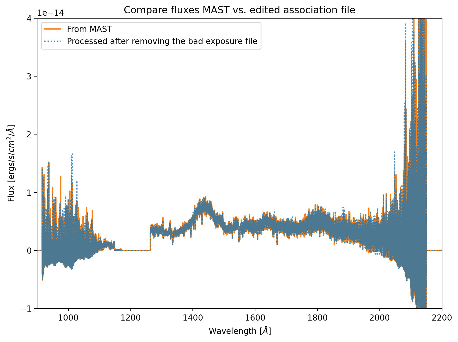
To show what would happen if we run CalCOS on this association file, we include Figure 1. This figure shows that the flux level of the spectrum retrieved from MAST matches that which was processed after removing the bad exposure. Slight differences in the two spectra may arise from MAST using a different random seed value. What matters for this comparison is that the fluxes match well, as they should because the empty exposure adds 0 counts over 0 time. Thus, for the purposes of flux calibration, it should be ignored. Other types of bad exposures, for instance those taken with the source at the edge of COS’s aperture, would impact the fluxes.

Figure 1. Comparison of fluxes between the data retrieved from MAST, and the same data reprocessed after removing the bad exposure#

A comparison between the fluxes of our data. One dataset if without our bad exposure removed, and the other is with our bad exposure removed. Both plots are relatively the same, as they should be.

2.1.2. Filtering to a single exposure (e.g. for LP6 data)#

Another situation when users often wish to remove exposures from an association file is when re-processing individual exposures taken at COS’s lifetime position 6 (LP6) or other modes at which the wavelength calibration data is not contained by the science exposures’ rawtag files.

Often users wish to process a single exposure’s file with CalCOS. With the TAGFLASH wavelength calibration method standard at all lifetime positions prior to LP6, the wavelength calibration data was taken concurrently with the science data and was contained by the same rawtag data files. However, as described in this COS 2030 plan poster, this is not possible at LP6. Instead, separate wavelength calibration exposures are taken at separate lifetime positions in a process known as SPLIT wavecals. As a result, the wavelength calibration data no longer exists in the same file as the science data for such exposures.

For TAGFLASH data, users could run CalCOS directly on their rawtag file of interest (though using an association file was always recommended). However, doing so with LP6 data would not allow the proper wavelength calibration. Instead, users should create a custom association file created by removing exposures from the default association file. We demonstrate this below.

We’ll alter an LP6 association file with the observation ID letc01010. Let’s begin by downloading the default LP6 association file from MAST and displaying it:

# Search for the correct obs_ids and get the list of data products
lp6_observation_products = Observations.get_product_list(
                                Observations.query_criteria(
                                    obs_id='letc01010'),
)

# Download the asnfile product list, then get the 0th element of the
# resulting path list, since there's only 1 asn file
lp6_original_asnfile = Path(
    Observations.download_products(
        Observations.filter_products(
            lp6_observation_products,
            productSubGroupDescription=['ASN'],
        ),
        download_dir=str(datadir)
    )['Local Path'][0]
)

# Show the default association file for the LP6 dataset.
Table.read(lp6_original_asnfile)

Downloading URL https://mast.stsci.edu/api/v0.1/Download/file?uri=mast:HST/product/letc01010_asn.fits to data/mastDownload/HST/letc01010/letc01010_asn.fits ...

 [Done]

Table length=13

MEMNAME	MEMTYPE	MEMPRSNT
bytes14	bytes14	bool
LETC01LMQ	EXP-SWAVE	1
LETC01LOQ	EXP-FP	1
LETC01LRQ	EXP-SWAVE	1
LETC01LTQ	EXP-SWAVE	1
LETC01LWQ	EXP-FP	1
LETC01M1Q	EXP-SWAVE	1
LETC01M6Q	EXP-SWAVE	1
LETC01MTQ	EXP-FP	1
LETC01MVQ	EXP-SWAVE	1
LETC01MXQ	EXP-SWAVE	1
LETC01MZQ	EXP-FP	1
LETC01N1Q	EXP-SWAVE	1
LETC01010	PROD-FP	1

As expected, we see 4 EXP-FP members, which are the science exposures at COS’s 4 fixed-pattern noise positions (FP-POS). Each is bracketed by a SPLIT wavecal wavelength calibration exposure on each side (EXP-SWAVE).

If we only wish to process one of the science exposures, (along with its wavelength calibration exposures,) we turn off all the other exposures by setting their MEMPRSNT values to 0/False. The product file (PROD-FP) must also be turned on, and should be renamed to show that it will only include data from a single exposure. Below, we do so, assuming we wish to process only the FP-POS = 3 science exposure: LETC01MTQ (and its wavelength calibration exposures: LETC01M6Q and LETC01MVQ).

# WAVECAL -> SCIENCE -> WAVECAL
exposures_to_use = ['LETC01M6Q', 'LETC01MTQ', 'LETC01MVQ']

print(f"We will turn off the input exposures except for: {exposures_to_use}."
      f" We will also leave the output product file turned on.")

# Make a copy of the original asn file with a name to
# indicate it will only process a single chosen exposure:
lp6_1exposure_asnfile = shutil.copy(lp6_original_asnfile,
                                    datadir / 'letc01mtq_only_asn.fits')

# Turn off all the other exposures in the copy
with fits.open(lp6_1exposure_asnfile, mode='update') as hdulist:
    tbdata = hdulist[1].data
    # Turn off files except those listed here
    for expfile in tbdata:
        # If file isn't what we're going to use, set MEMPRSNT to False AKA 0
        if expfile['MEMNAME'] not in exposures_to_use:
            expfile['MEMPRSNT'] = False
        # Turn on and rename the product file to indicate
        # it will only include the chosen exposure:
        if expfile['MEMTYPE'] == 'PROD-FP':
            # Turn on the product file
            expfile['MEMPRSNT'] = True
            # Rename the product file
            expfile['MEMNAME'] = "LETC01MTQ_only"

# Re-read the table to see the change
Table.read(lp6_1exposure_asnfile)

We will turn off the input exposures except for: ['LETC01M6Q', 'LETC01MTQ', 'LETC01MVQ']. We will also leave the output product file turned on.

Table length=13

MEMNAME	MEMTYPE	MEMPRSNT
bytes14	bytes14	bool
LETC01LMQ	EXP-SWAVE	0
LETC01LOQ	EXP-FP	0
LETC01LRQ	EXP-SWAVE	0
LETC01LTQ	EXP-SWAVE	0
LETC01LWQ	EXP-FP	0
LETC01M1Q	EXP-SWAVE	0
LETC01M6Q	EXP-SWAVE	1
LETC01MTQ	EXP-FP	1
LETC01MVQ	EXP-SWAVE	1
LETC01MXQ	EXP-SWAVE	0
LETC01MZQ	EXP-FP	0
LETC01N1Q	EXP-SWAVE	0
LETC01MTQ_only	PROD-FP	1

2.2. Adding an exposure#

In section 2.1.1, we removed the failed exposure taken with FP-POS = 1 from our ldif01010 association file. When possible, we usually want to combine one or more of each of the four FP-POS types. In this example scenario, let’s add the FP-POS = 1 exposure from the other association group. Please note that combining data from separate visits with different target acquisitions can result in true errors which are higher than those calculated by CalCOS. We combine the datasets here as an example only and do not specifically endorse combining these exposures. Also note that you should only combine files taken using the same grating and central wavelength settings in this manner.

In the cell below, we determine which exposure from LDIF02010 was taken with FP-POS = 1.

It does this by looping through the files listed in LDIF02010’s association file, and then reading in that file’s header to check if its FPPOS = 1.
It also prints some diagnostic information about all of the exposure files.

# Reads the contents of the 2nd asn file
asn_con_2 = Table.read(asnfiles[1])

# Loops through each file in asn table for `LDIF02010`
for memname, memtype in zip(asn_con_2['MEMNAME'], asn_con_2["MEMTYPE"]):
    # Convert file names to lower case letters, as in actual filenames
    memname = memname.lower()
    # We only want to look at the exposure files
    if memtype == 'EXP-FP':
        # Search for the actual filepath of the memname for rawtag_a & rawtag_b
        rt_a = (glob.glob(f"**/*{memname}*rawtag_a*", recursive=True))[0]
        rt_b = (glob.glob(f"**/*{memname}*rawtag_b*", recursive=True))[0]

        # Now print all these diagnostics:
        print(f"Association {(fits.getheader(rt_a))['ASN_ID']} has {memtype} "
              f"exposure {memname.upper()} with "
              f"exptime {(fits.getheader(rt_a, ext=1))['EXPTIME']} seconds"
              f" at cenwave {(fits.getheader(rt_a, ext=0))['CENWAVE']} Å and "
              f"FP-POS {(fits.getheader(rt_a, ext=0))['FPPOS']}.")

        # Checking if the file is FP-POS = 1
        if (fits.getheader(rt_a, ext=0))['FPPOS'] == 1:
            print(f"^^ The one above this has the FP-POS "
                  f"we are looking for ({memname.upper()})^^^\n")
            # Save the right file basename in a variable
            asn2_fppos1_name = memname.upper()

Association LDIF02010 has EXP-FP exposure LDIF02NMQ with exptime 1653.0 seconds at cenwave 1280 Å and FP-POS 1.
^^ The one above this has the FP-POS we are looking for (LDIF02NMQ)^^^

Association LDIF02010 has EXP-FP exposure LDIF02NSQ with exptime 1334.0 seconds at cenwave 1280 Å and FP-POS 2.
Association LDIF02010 has EXP-FP exposure LDIF02NUQ with exptime 1334.0 seconds at cenwave 1280 Å and FP-POS 3.
Association LDIF02010 has EXP-FP exposure LDIF02NWQ with exptime 2783.0 seconds at cenwave 1280 Å and FP-POS 4.

There’s a slightly different procedure to add a new exposure to the list rather than remove one.

Here we will read the table in the FITS association file into an astropy Table. We can then add a row into the right spot, filling it with the new file’s MEMNAME, MEMTYPE, and MEMPRSNT. Finally, we have to save this table into the existing FITS association file.

# Read in original data from the file
asn_orig_table = Table.read(asnfile)

# Add a row with the right name after all the original EXP-FP's
asn_orig_table.insert_row(len(asn_orig_table) - 1,
                          [asn2_fppos1_name, 'EXP-FP', 1])

# Turn this into a FITS Binary Table HDU
new_table = fits.BinTableHDU(asn_orig_table)

# We need to change data with the asnfile opened and in 'update' mode
with fits.open(asnfile, mode='update') as hdulist:
    # Change the orig file's data to the new table data we made
    hdulist[1].data = new_table.data

print(f"Added {asn2_fppos1_name} to the association file.")

Added LDIF02NMQ to the association file.

Now, we can see there is a new row with our exposure from the other asn file group: LDIF02NMQ.

Table.read(asnfile)

Table length=6

MEMNAME	MEMTYPE	MEMPRSNT
bytes14	bytes14	bool
LDIF01TYQ	EXP-FP	0
LDIF01U0Q	EXP-FP	1
LDIF01U2Q	EXP-FP	1
LDIF01U4Q	EXP-FP	1
LDIF02NMQ	EXP-FP	1
LDIF01010	PROD-FP	1

Excellent. In the next section we will create a new association file from scratch.

3. Creating an entirely new association file#

Users will rarely need to create an entirely new association file. Much more often, they should alter an existing one found on MAST. However, a user may wish to create a new association file if they are combining altered exposures, perhaps after using the costools.splittag tool. This section describes how to make one from scratch.

For the sake of demonstration, we will generate a new association file with four exposure members: even-numbered FP-POS (2,4) from the first original association (LDIF01010), and odd-numbered FP-POS (1,3) from from the second original association (LDIF02010).

From Section 2, we see that this corresponds to :

Name	Original asn	FP-POS
LDIF02010	LDIF02NMQ	1
LDIF01010	LDIF01U0Q	2
LDIF02010	LDIF02NUQ	3
LDIF01010	LDIF01U4Q	4

3.1. Simplest method#

Below, we manually build up an association file from the three necessary columns (MEMNAME, MEMTYPE, MEMPRSNT).

# Adding the exposure file details to the association table
# MEMNAME:
new_asn_memnames = ['LDIF02NMQ', 'LDIF01U0Q', 'LDIF02NUQ', 'LDIF01U4Q']
# MEMTYPE:
types = ['EXP-FP', 'EXP-FP', 'EXP-FP', 'EXP-FP']
# MEMPRSNT
included = [True, True, True, True]

# Adding the ASN details to the end of the association table
# MEMNAME column:
new_asn_memnames.append('ldifcombo'.upper())
# MEMTYPE column:
types.append('PROD-FP')
# MEMPRSNT column
included.append(True)

# Putting together the FITS table:
#   40 is the number of characters allowed in this
#   field with the MEMNAME format = 40A. If your rootname
#   is longer than 40, you will need to increase this.
c1 = fits.Column(name='MEMNAME',
                 array=np.array(new_asn_memnames),
                 format='40A')

c2 = fits.Column(name='MEMTYPE',
                 array=np.array(types),
                 format='14A')

c3 = fits.Column(name='MEMPRSNT',
                 format='L',
                 array=included)

asn_table = fits.BinTableHDU.from_columns([c1, c2, c3])

# Writing the fits table
asn_table.writeto(outputdir / 'ldifcombo_asn.fits', overwrite=True)

print('Saved ' + 'ldifcombo_asn.fits'
      + f" in the output directory: {outputdir}")

Saved ldifcombo_asn.fits in the output directory: output

Examining the file we have created:

We see that the data looks correct - exactly the table we want!

Table.read(outputdir / 'ldifcombo_asn.fits')

Table length=5

MEMNAME	MEMTYPE	MEMPRSNT
bytes40	bytes14	bool
LDIF02NMQ	EXP-FP	True
LDIF01U0Q	EXP-FP	True
LDIF02NUQ	EXP-FP	True
LDIF01U4Q	EXP-FP	True
LDIFCOMBO	PROD-FP	True

However, the 0th and 1st fits headers no longer contain useful information about the data. While CalCOS will process these files, vital header keys may not be propagated. If it’s important to preserve the header information, you may follow the steps in the next section.

fits.getheader(outputdir / 'ldifcombo_asn.fits', ext=0)

SIMPLE  =                    T / conforms to FITS standard                      
BITPIX  =                    8 / array data type                                
NAXIS   =                    0 / number of array dimensions                     
EXTEND  =                    T                                                  

fits.getheader(outputdir / 'ldifcombo_asn.fits', ext=1)

XTENSION= 'BINTABLE'           / binary table extension                         
BITPIX  =                    8 / array data type                                
NAXIS   =                    2 / number of array dimensions                     
NAXIS1  =                   55 / length of dimension 1                          
NAXIS2  =                    5 / length of dimension 2                          
PCOUNT  =                    0 / number of group parameters                     
GCOUNT  =                    1 / number of groups                               
TFIELDS =                    3 / number of table fields                         
TTYPE1  = 'MEMNAME '                                                            
TFORM1  = '40A     '                                                            
TTYPE2  = 'MEMTYPE '                                                            
TFORM2  = '14A     '                                                            
TTYPE3  = 'MEMPRSNT'                                                            
TFORM3  = 'L       '                                                            

3.2. With FITS header metadata#

We can instead build up a new file with our old file’s FITS header, and alter it to reflect our changes.

We first build a new association file, a piecewise combination of our original file’s headers and our new table.

A FITS header is essentially a section of data and its associated metadata. See this site for info on FITS structures.

# Open up the old asn file
with fits.open(asnfile, mode='readonly') as hdulist:
    # Shows the first hdu is empty except for the header we want
    hdulist.info()
    # We want to directly copy over the old 0th header/data-unit AKA "hdu".
    hdu0 = hdulist[0]
    # Gather the data from the header/data unit to allow the readout
    d0 = hdulist[0].data
    # Gather the header from the 1st header/data unit to copy to our new file
    h1 = hdulist[1].header

# Put together new 1st hdu from old header and new data
hdu1 = fits.BinTableHDU.from_columns([c1, c2, c3],
                                     header=h1)

# New HDUList from old HDU 0 and new combined HDU 1
new_HDUlist = fits.HDUList([hdu0, hdu1])

# Write this out to a new file
new_HDUlist.writeto(outputdir / 'ldifcombo_2_asn.fits',
                    overwrite=True)
# Path to this new file
new_asnfile = outputdir / 'ldifcombo_2_asn.fits'

print('\nSaved ' + 'ldifcombo_2_asn.fits'
      + f"in the output directory: {outputdir}")

Filename: data/ldif01010_asn.fits
No.    Name      Ver    Type      Cards   Dimensions   Format
  0  PRIMARY       1 PrimaryHDU      43   ()      
  1  ASN           1 BinTableHDU     24   6R x 3C   [14A, 14A, L]   

Saved ldifcombo_2_asn.fitsin the output directory: output

Now we edit the relevant values in our FITS headers that are different from the original.

Note: It is possible that a generic FITS file may have different values you may wish to change. It is highly recommended to examine your FITS headers.

# Find today's date
date = datetime.date.today()
# Below, make a dict of what header values we want to change,
# corresponding to [new value, ext. the value lives in, 2nd ext. if applies]
keys_to_change = {'DATE': [f'{date.year}-{date.month}-{date.day}', 0],
                  'FILENAME': ['ldifcombo_2_asn.fits', 0],
                  'ROOTNAME': ['ldifcombo_2', 0, 1],
                  'ASN_ID': ['ldifcombo_2', 0],
                  'ASN_TAB': ['ldifcombo_2_asn.fits', 0],
                  'ASN_PROD': ['False', 0],
                  'EXTVER': [2, 1],
                  'EXPNAME': ['ldifcombo_2', 1]}

# Actually change the values below (verbosely):
for keyval in keys_to_change.items():
    print(f"Editing {keyval[0]} in Extension {keyval[1][1]}")
    fits.setval(filename=new_asnfile,
                keyword=keyval[0],
                value=keyval[1][0],
                ext=keyval[1][1])
    
    # Below is necessary as some keys are repeated in both headers ('ROOTNAME')
    if len(keyval[1]) > 2:
        print(f"Editing {keyval[0]} in Extension {keyval[1][2]}")
        fits.setval(filename=new_asnfile,
                    keyword=keyval[0],
                    value=keyval[1][0],
                    ext=keyval[1][2])

Editing DATE in Extension 0
Editing FILENAME in Extension 0
Editing ROOTNAME in Extension 0
Editing ROOTNAME in Extension 1
Editing ASN_ID in Extension 0
Editing ASN_TAB in Extension 0
Editing ASN_PROD in Extension 0
Editing EXTVER in Extension 1
Editing EXPNAME in Extension 1

And now we have created our new association file. The file is now ready to be used in the CalCOS pipeline!

If you’re interested in testing your file by running it through the CalCOS pipeline, you may wish to run the test_asn.py file included in this subdirectory of the GitHub repository. i.e. from the command line:

$ python test_asn.py

Note that you must first…

Have created the file by running this Notebook
Alter line 21 of test_asn.py to set the lref directory to wherever you have your cache of CRDS reference files (see our Setup Notebook).

If the test runs successfully, it will create a plot in the subdirectory ./output/plots/ .

3.3. Association files for non-TAGFLASH datasets#

As touched upon in Section 2.1.2., most COS exposures contain the calibration lamp data necessary to perform wavelength calibration; however, exposures taken at LP6 and those taken with AUTO and GO wavecals (including BOA and ACCUM mode exposures) have separate exposures for wavelength calibration. Table 1 below summarizes the types of wavelength calibration modes. More information may be found in Section 5.7 of the COS Instrument Handbook.

Table 1. Comparison of wavelength calibration modes#

Wavelength calibration mode	`TAGFLASH`	`SPLIT` Wavecal	`AUTO` Wavecal	GO Wavecal
When used	Default for LP1-LP5	Default for LP6	Used for LP1-LP5 non-TAGFLASH exposures	User specified (rare)
Description	Wavelength calibration lamp flashes concurrently with science exposure	Wavelength calibration lamp flashes at another LP	Wavelength calibration lamp flashes separately from science exposure	Wavelength calibration lamp flashes separately from science exposure
Additional wavelength calibration file in the association table	None - wavelength calibration data included in the `EXP-FP`s of the science exposures	`EXP-SWAVE`	`EXP-AWAVE`	`EXP-GWAVE`

Non-TAGFLASH datasets must be processed from a single association file which includes all the science and wavelength calibration exposures, properly labeled with the correct MEMTYPEs.

Users will rarely need to build an entirely new association file for non-TAGFLASH datasets. The most common reason for a user to have non-TAGFLASH data is that the exposures were obtained using the SPLIT wavecal method at LP6. The association files for these files are correctly created and made available in the MAST archive. Removing specific exposures can most easily be done as in Section 2.1.2. However, if a user needed to craft a completely customized CalCOS run, for instance to combine multiple non-TAGFLASH datasets, they can follow this section.

In this section we will manually recreate the association file for the SPLIT wavecal data from the same dataset whose association file we altered as part of Section 2.1.2. We could just as easily do so with AUTO or GO wavecal data. We will first select and examine the relevant exposures, then we will combine them into an association file.

3.3.1. Gathering the exposure information#

We begin by downloading the data from a visit which utilized COS’ LP6 split wavecal mode (proposal ID: 16907, observation ID: letc01010). We previously downloaded the association file for this dataset in Section 2.1.2, but here we download the rest of the data products we will need.

# Search for the correct obs_ids and get the list of data products
lp6_observation_products = Observations.get_product_list(
                                    Observations.query_criteria(
                                        obs_id='letc01010'),
)

# Filter & download the rawtag files and asn file in the product list from MAST
# First filter to just the rawtag products
lp6_rawtags_pl = Observations.filter_products(
                    lp6_observation_products,
                    productSubGroupDescription=['RAWTAG_A', 'RAWTAG_B'])

# Download these chosen rawtag products
lp6_rawtags = Observations.download_products(
                                    lp6_rawtags_pl,
                                    download_dir=str(datadir))['Local Path']

Downloading URL https://mast.stsci.edu/api/v0.1/Download/file?uri=mast:HST/product/letc01lmq_rawtag_a.fits to data/mastDownload/HST/letc01lmq/letc01lmq_rawtag_a.fits ...

 [Done]

Downloading URL https://mast.stsci.edu/api/v0.1/Download/file?uri=mast:HST/product/letc01lmq_rawtag_b.fits to data/mastDownload/HST/letc01lmq/letc01lmq_rawtag_b.fits ...

 [Done]

Downloading URL https://mast.stsci.edu/api/v0.1/Download/file?uri=mast:HST/product/letc01loq_rawtag_a.fits to data/mastDownload/HST/letc01loq/letc01loq_rawtag_a.fits ...

 [Done]

Downloading URL https://mast.stsci.edu/api/v0.1/Download/file?uri=mast:HST/product/letc01loq_rawtag_b.fits to data/mastDownload/HST/letc01loq/letc01loq_rawtag_b.fits ...

 [Done]

Downloading URL https://mast.stsci.edu/api/v0.1/Download/file?uri=mast:HST/product/letc01lrq_rawtag_a.fits to data/mastDownload/HST/letc01lrq/letc01lrq_rawtag_a.fits ...

 [Done]

Downloading URL https://mast.stsci.edu/api/v0.1/Download/file?uri=mast:HST/product/letc01lrq_rawtag_b.fits to data/mastDownload/HST/letc01lrq/letc01lrq_rawtag_b.fits ...

 [Done]

Downloading URL https://mast.stsci.edu/api/v0.1/Download/file?uri=mast:HST/product/letc01ltq_rawtag_a.fits to data/mastDownload/HST/letc01ltq/letc01ltq_rawtag_a.fits ...

 [Done]

Downloading URL https://mast.stsci.edu/api/v0.1/Download/file?uri=mast:HST/product/letc01ltq_rawtag_b.fits to data/mastDownload/HST/letc01ltq/letc01ltq_rawtag_b.fits ...

 [Done]

Downloading URL https://mast.stsci.edu/api/v0.1/Download/file?uri=mast:HST/product/letc01lwq_rawtag_a.fits to data/mastDownload/HST/letc01lwq/letc01lwq_rawtag_a.fits ...

 [Done]

Downloading URL https://mast.stsci.edu/api/v0.1/Download/file?uri=mast:HST/product/letc01lwq_rawtag_b.fits to data/mastDownload/HST/letc01lwq/letc01lwq_rawtag_b.fits ...

 [Done]

Downloading URL https://mast.stsci.edu/api/v0.1/Download/file?uri=mast:HST/product/letc01m1q_rawtag_a.fits to data/mastDownload/HST/letc01m1q/letc01m1q_rawtag_a.fits ...

 [Done]

Downloading URL https://mast.stsci.edu/api/v0.1/Download/file?uri=mast:HST/product/letc01m1q_rawtag_b.fits to data/mastDownload/HST/letc01m1q/letc01m1q_rawtag_b.fits ...

 [Done]

Downloading URL https://mast.stsci.edu/api/v0.1/Download/file?uri=mast:HST/product/letc01m6q_rawtag_a.fits to data/mastDownload/HST/letc01m6q/letc01m6q_rawtag_a.fits ...

 [Done]

Downloading URL https://mast.stsci.edu/api/v0.1/Download/file?uri=mast:HST/product/letc01m6q_rawtag_b.fits to data/mastDownload/HST/letc01m6q/letc01m6q_rawtag_b.fits ...

 [Done]

Downloading URL https://mast.stsci.edu/api/v0.1/Download/file?uri=mast:HST/product/letc01mtq_rawtag_a.fits to data/mastDownload/HST/letc01mtq/letc01mtq_rawtag_a.fits ...

 [Done]

Downloading URL https://mast.stsci.edu/api/v0.1/Download/file?uri=mast:HST/product/letc01mtq_rawtag_b.fits to data/mastDownload/HST/letc01mtq/letc01mtq_rawtag_b.fits ...

 [Done]

Downloading URL https://mast.stsci.edu/api/v0.1/Download/file?uri=mast:HST/product/letc01mvq_rawtag_a.fits to data/mastDownload/HST/letc01mvq/letc01mvq_rawtag_a.fits ...

 [Done]

Downloading URL https://mast.stsci.edu/api/v0.1/Download/file?uri=mast:HST/product/letc01mvq_rawtag_b.fits to data/mastDownload/HST/letc01mvq/letc01mvq_rawtag_b.fits ...

 [Done]

Downloading URL https://mast.stsci.edu/api/v0.1/Download/file?uri=mast:HST/product/letc01mxq_rawtag_a.fits to data/mastDownload/HST/letc01mxq/letc01mxq_rawtag_a.fits ...

 [Done]

Downloading URL https://mast.stsci.edu/api/v0.1/Download/file?uri=mast:HST/product/letc01mxq_rawtag_b.fits to data/mastDownload/HST/letc01mxq/letc01mxq_rawtag_b.fits ...

 [Done]

Downloading URL https://mast.stsci.edu/api/v0.1/Download/file?uri=mast:HST/product/letc01mzq_rawtag_a.fits to data/mastDownload/HST/letc01mzq/letc01mzq_rawtag_a.fits ...

 [Done]

Downloading URL https://mast.stsci.edu/api/v0.1/Download/file?uri=mast:HST/product/letc01mzq_rawtag_b.fits to data/mastDownload/HST/letc01mzq/letc01mzq_rawtag_b.fits ...

 [Done]

Downloading URL https://mast.stsci.edu/api/v0.1/Download/file?uri=mast:HST/product/letc01n1q_rawtag_a.fits to data/mastDownload/HST/letc01n1q/letc01n1q_rawtag_a.fits ...

 [Done]

Downloading URL https://mast.stsci.edu/api/v0.1/Download/file?uri=mast:HST/product/letc01n1q_rawtag_b.fits to data/mastDownload/HST/letc01n1q/letc01n1q_rawtag_b.fits ...

 [Done]

We’ll begin by taking a look at the original association file from MAST in the cell below. Note that the exposures are ordered in groups of a single EXP-FP (also known as science or EXTERNAL/SCI) exposure bracketed on both sides by an EXP-SWAVE (SPLIT wavecal) exposure (i.e. WAVECAL–> SCIENCE –> WAVECAL). This is often the case for non-TAGFLASH files, especially for exposures longer than ~600 seconds.

Table.read(lp6_original_asnfile)

Table length=13

MEMNAME	MEMTYPE	MEMPRSNT
bytes14	bytes14	bool
LETC01LMQ	EXP-SWAVE	1
LETC01LOQ	EXP-FP	1
LETC01LRQ	EXP-SWAVE	1
LETC01LTQ	EXP-SWAVE	1
LETC01LWQ	EXP-FP	1
LETC01M1Q	EXP-SWAVE	1
LETC01M6Q	EXP-SWAVE	1
LETC01MTQ	EXP-FP	1
LETC01MVQ	EXP-SWAVE	1
LETC01MXQ	EXP-SWAVE	1
LETC01MZQ	EXP-FP	1
LETC01N1Q	EXP-SWAVE	1
LETC01010	PROD-FP	1

We’ll simulate an occasion on which we would need to create our own association file by supposing we want to process only data from this observation taken in the FP-POS = 1 or FP-POS = 3 configuration. We could achieve the same result by taking the default association file from MAST and turning the MEMPRSNT value to False for all the FP-POS = 2 and FP-POS = 4 files, similarly to in Section 2.1.2.

Below, we filter to such exposures and check whether they meet our expectations for SPLIT wavecal data. Namely, we check that:

The files are listed in chronological order.
All science (EXTERNAL/SCI) exposures are bracketed by a WAVECAL exposure on either side.
The data is organized into groups of 3 exposures with the grouping described in test 2 (WAVECAL–>EXTERNAL/SCI–>WAVECAL).

CalCOS does not strictly need the files to be arranged in chronological order; however, it is a helpful exercise to make sure we include all the files we need to calibrate this dataset. We can investigate the files manually and diagnose any failures in the table printed by the following cell.

# Filter the rawtag files to exposures at FP1 and FP3
lp6_rawtags_fp13 = [rt for rt in lp6_rawtags
                    if fits.getval(rt, "FPPOS", ext=0) in [1, 3]]

# Gather information on all the exposures
rawtag_a_exptypes_dict = {rt: fits.getval(rt, "EXPTYPE", ext=0)
                          for rt in lp6_rawtags_fp13 if "rawtag_a" in rt}

rawtag_a_rootnames = [fits.getval(rt, "ROOTNAME", ext=0)
                      for rt in lp6_rawtags_fp13 if "rawtag_a" in rt]

rawtag_a_exptypes = [fits.getval(rt, "EXPTYPE", ext=0)
                     for rt in lp6_rawtags_fp13 if "rawtag_a" in rt]

rawtag_a_expstart_times = [fits.getval(rt, "EXPSTART", ext=1)
                           for rt in lp6_rawtags_fp13 if "rawtag_a" in rt]

# Test 1
# Check chronological sorting
assert all(np.diff(rawtag_a_expstart_times) >= 0), "These exposures are not ordered by start time."
print("Passed Test #1: The exposures are in chronological order.")

# Test 2
# Check science exposures are bracketed by wavecals
for i, rta_type in enumerate(rawtag_a_exptypes):
    if rta_type == "EXTERNAL/SCI":
        assert rawtag_a_exptypes[i-1] == "WAVECAL", "EXTERNAL/SCI exposure not preceded by a WAVECAL exposure"
        assert rawtag_a_exptypes[i+1] == "WAVECAL", "EXTERNAL/SCI exposure not followed by a WAVECAL exposure"
print("Passed Test #2: Each EXTERNAL/SCI is bracketted on both sides by a WAVECAL exposure.")

# Test 3 
# Check that only these groups of exposures exist (WAVECAL-->EXTERNAL/SCI-->WAVECAL)
for group_of_3 in [rawtag_a_exptypes[3*i:3*i+3] for i in range(int(len(rawtag_a_exptypes)/3))]:
    assert group_of_3 == ['WAVECAL', 'EXTERNAL/SCI', 'WAVECAL'], "Incorrect groupings of exposures"
print("Passed Test #3: No unexpected groupings of files were found.")

Passed Test #1: The exposures are in chronological order.
Passed Test #2: Each EXTERNAL/SCI is bracketted on both sides by a WAVECAL exposure.
Passed Test #3: No unexpected groupings of files were found.

Below, we may inspect these files by eye, and see that they are indeed ordered correctly.

pd.DataFrame({
    "Rootname": [name.upper() for name in rawtag_a_rootnames], 
    "Exposure_type": rawtag_a_exptypes,
    # Date in MJD
    "Exposure_start_date": rawtag_a_expstart_times,
    "Seconds_since_first_exposure": \
    # Convert time since the first exposure into seconds
    86400*np.subtract(rawtag_a_expstart_times, min(rawtag_a_expstart_times))
})

	Rootname	Exposure_type	Exposure_start_date	Seconds_since_first_exposure
0	LETC01LMQ	WAVECAL	59648.009183	0.000000
1	LETC01LOQ	EXTERNAL/SCI	59648.010537	116.991648
2	LETC01LRQ	WAVECAL	59648.019426	884.991744
3	LETC01M6Q	WAVECAL	59648.045549	3142.016352
4	LETC01MTQ	EXTERNAL/SCI	59648.065745	4887.007776
5	LETC01MVQ	WAVECAL	59648.074634	5655.007872

Once we are sure that the correct exposures are selected, we gather the information we need for an association table:

The exposure ID (ROOTNAME) of each exposure.
- When capitalized, this is the same as the MEMNAME we find in association files.
The exposure type (EXPTYPE) of each exposure.
- We will need to convert from the way that exposure types are written in the FITS header to the way CalCOS will recognize them in the association file.

To prevent duplication, we only gather this information from either the rawtag_a or rawtag_b files.

# Choose either rawtag_a (default) of rawtag_b files if no rawtag_a files found
if any(["rawtag_a" in rt for rt in lp6_rawtags_fp13]):
    seg_found = "a"
elif any(["rawtag_b" in rt for rt in lp6_rawtags_fp13]):
    seg_found = "b"
else:
    print("Neither rawtag_a nor rawtag_b found.")

lp6_fp13_memnames = [fits.getval(rt, "ROOTNAME", ext=0).upper()
                     for rt in lp6_rawtags_fp13 if f"rawtag_{seg_found}" in rt]

lp6_fp13_exptypes = [fits.getval(rt, "EXPTYPE", ext=0)
                     for rt in lp6_rawtags_fp13 if f"rawtag_{seg_found}" in rt]

# We need to change the wavecals' MEMTYPE to "EXP-SWAVE"
# and the sciences' to "EXP-FP":
lp6_fp13_exptypes = [
    "EXP-SWAVE" if etype == "WAVECAL"
    else "EXP-FP" if etype == "EXTERNAL/SCI"
    else None for etype in lp6_fp13_exptypes
]
print("Gathered exposure information for creating a new non-TAGFLASH association file.")

Gathered exposure information for creating a new non-TAGFLASH association file.

3.3.2. Creating the `SPLIT` wavecal association file#

Now that we’ve gathered MEMNAMEs and MEMTYPEs of our exposures, we can create the association file. This very closely mirrors Section 3.2.

# Adding the exposure file details to the association table
# MEMNAME:
new_asn_memnames = lp6_fp13_memnames
# MEMTYPE
types = lp6_fp13_exptypes
# MEMPRSNT
included = [True] * len(lp6_fp13_memnames)

# Adding the output science product details to the
# end of the association table columns:

# MEMNAME column:
new_asn_memnames.append('splitwave'.upper())
# MEMTYPE column:
types.append('PROD-FP')
# MEMPRSNT column:
included.append(True)

# Convert the columns into a the necessary form for a FITS file
c1 = fits.Column(name='MEMNAME',
                 array=np.array(new_asn_memnames),
                 format='40A')

c2 = fits.Column(name='MEMTYPE',
                 array=np.array(types),
                 format='14A')

c3 = fits.Column(name='MEMPRSNT',
                 format='L',
                 array=included)

# Open up the old asn file:
with fits.open(lp6_original_asnfile, mode='readonly') as hdulist:
    # Shows the first hdu is empty except for the header we want
    hdulist.info()
    # We want to directly copy over the old 0th header/data-unit
    hdu0 = hdulist[0]
    # Gather the data from the header/data unit to allow the readout
    d0 = hdulist[0].data
    # Gather the header from the 1st header/data unit to copy to our new file
    h1 = hdulist[1].header

# Put together new 1st hdu from old header and new data
hdu1 = fits.BinTableHDU.from_columns([c1, c2, c3],
                                     header=h1)

# New HDUList from old HDU 0 and new combined HDU 1
new_HDUlist = fits.HDUList([hdu0, hdu1])

# Write this out to a new file
new_HDUlist.writeto(outputdir / 'splitwave_asn.fits', overwrite=True)
# Path to this new file
new_asnfile = outputdir / 'splitwave_asn.fits'

print('\nSaved ' + 'splitwave_asn.fits'
      f" in the output directory: {outputdir}")

Filename: data/mastDownload/HST/letc01010/letc01010_asn.fits
No.    Name      Ver    Type      Cards   Dimensions   Format
  0  PRIMARY       1 PrimaryHDU      43   ()      
  1  ASN           1 BinTableHDU     25   13R x 3C   [14A, 14A, L]   

Saved splitwave_asn.fits in the output directory: output

Table.read(outputdir/"splitwave_asn.fits")

Table length=7

MEMNAME	MEMTYPE	MEMPRSNT
bytes40	bytes14	bool
LETC01LMQ	EXP-SWAVE	True
LETC01LOQ	EXP-FP	True
LETC01LRQ	EXP-SWAVE	True
LETC01M6Q	EXP-SWAVE	True
LETC01MTQ	EXP-FP	True
LETC01MVQ	EXP-SWAVE	True
SPLITWAVE	PROD-FP	True

Well done - you have now successfully created the association file you need to process your SPLIT wavecal data. If you wish to test it by running the CalCOS data calibration pipeline on it, you may run the file test_splitwave_asn.py in this directory. Note the following requirements:

test_splitwave_asn.py can only be run after creating the asn files in Section 3.3 of this Notebook.
Your version of CalCOS must be ≥ 3.4. This version introduced the ability to process SPLIT wavecal data to the pipeline. You can check your version with calcos --version from the command line.
You must first update the lref environment variable set in test_splitwave_asn.py to the path to a directory containing all of your reference files. For more information on setting up such a directory, see our Notebook on setting up an environment for COS data analysis.

Congratulations! You finished this Notebook!#

There are more COS data walkthrough Notebooks on different topics. You can find them here.

About this Notebook#

Author: Nat Kerman: nkerman@stsci.edu

Contributors: Elaine Mae Frazer, Travis Fischer

Updated On: 2023-03-27

This tutorial was generated to be in compliance with the STScI style guides and would like to cite the Jupyter guide in particular.

Citations#

If you use astropy, matplotlib, astroquery, or numpy for published research, please cite the authors. Follow these links for more information about citations:

Top of Page

Modifying or Creating an Association File

Contents

Modifying or Creating an Association File#

Learning Goals#

0. Introduction#

We will import the following packages:#

We will also define a few directories we will need:#

And we will need to download the data we wish to filter and analyze#

1. Examining an association file#

2. Editing an existing association file#

2.1. Removing an exposure#

2.1.1. Removing a bad exposure#

Figure 1. Comparison of fluxes between the data retrieved from MAST, and the same data reprocessed after removing the bad exposure#

2.1.2. Filtering to a single exposure (e.g. for LP6 data)#

2.2. Adding an exposure#

3. Creating an entirely new association file#

3.1. Simplest method#

3.2. With FITS header metadata#

3.3. Association files for non-TAGFLASH datasets#

Table 1. Comparison of wavelength calibration modes#

3.3.1. Gathering the exposure information#

3.3.2. Creating the SPLIT wavecal association file#

Congratulations! You finished this Notebook!#

About this Notebook#

Citations#

3.3.2. Creating the `SPLIT` wavecal association file#