
Drizzling new WFPC2 FLT data products with chip-normalization#
Table of Contents#
1. Introduction
2. Download the Data
3. Update the WCS
4. Align the Images
5. Drizzle-combine the images
Conclusions
1. Introduction #
This notebook shows how to work with a new type of WFPC2 calibrated data product in MAST. The new data products combine the previously separate files containing the science array c0m.fitsand data quality array c1m.fits into a new file with suffix flt.fits, similar to calibrated images for ACS and WFC3.
These flt files have now been corrected for differences in the inverse sensitivity the science arrays of each chip using the software ‘photeq’ so that a single PHOTFLAM (or PHOTFNU) value may be used for photometry.
The new flt files include four key differences from the older style c0m, c1m WFPC2 files:
1.) The SCI & DQ arrays are merged into a single file with multiple extensions.
2.) The SCI arrays are corrected for different 'inverse sensitivities' across chips.
3.) The SCI arrays from different chips may now be drizzled together in a mosaic.
4.) The SCI header WCS includes improved absolute astromentry (i.e. WCSNAME='*GAIA*').
This example uses WFPC2 observations of Omega Centauri (NGC 5139) in the F555W filter taken from CAL proposal 8447. The two exposures have been dithered to place the same stars on the WF2 and WF4 chips to measure relative photometry across the two chips. After using TweakReg to realign the images, we show how to combine the images with AstroDrizzle. We inspect the resulting science and weight images and compare the results with those derived from the older MAST data products.
Acronyms:
Hubble Space Telescope (HST)
Wide Field Camera 3 (WFC3)
Advanced Camera for Surveys (ACS)
Wide Field and Planetary Camera 2 (WFPC2)
Mikulski Archive for Space Telescopes (MAST)
Flexible Image Transport System (FITS)
World Coordinate System (WCS)
Hubble Advanced Products (HAP)
Single Visit Mosaic (SVM)
Planetary Chip (PC)
Import Packages#
The following Python packages are required to run the Jupyter Notebook:
os - change and make directories
glob - gather lists of filenames
shutil - copy files between folders
numpy - math and array functions
matplotlib - create graphics
pyplot - make figures and graphics
astroquery - download astronomical data
mast.Observations - query MAST database
astropy - model fitting and file handling
io.fits - import FITS files
table.Table - tables without physical units
visualization.LogStretch - display image normalization
visualization.ImageNormalize - display image normalization
ipython - cell formatting and interactives
display.Image - display image files
display.clear_output - clear text from cells
photutils - aperture photometry tools
photutils.aperture - aperture photometry tools
aperture_photometry - measure aperture photometry
CircularAperture - measure photometry in circle
CircularAnnulus - measure photometry in annulus
ApertureStats - calculate aperture statistics
drizzlepac - combine HST images into mosaics
astrodrizzle - combine exposures by drizzling
tweakreg - align exposures to a common WCS
stwcs - WCS based distortion models and transformations
updatewcs - modify WCS in HST file headers
import os
import glob
import shutil
import numpy as np
import matplotlib.pyplot as plt
from astroquery.mast import Observations
from astropy.table import Table
from astropy.io import fits
from astropy.visualization import LogStretch, ImageNormalize
from IPython.display import Image, clear_output
from photutils.aperture import CircularAnnulus, CircularAperture, ApertureStats, aperture_photometry
from drizzlepac import tweakreg, astrodrizzle
from stwcs.updatewcs import updatewcs

%matplotlib inline
%config InlineBackend.figure_format = 'retina'
2. Download the Data #
The WFPC2 data are downloaded using the astroquery API to access the MAST archive. The astroquery.mast documentation has more examples for how to find and download data from MAST.
MAST queries may be done using query_criteria, where we specify:
\(\rightarrow\) obs_id, proposal_id, and filters
MAST data products may be downloaded by using download_products, where we specify:
\(\rightarrow\) data_prod = original c0m, c1m files and new flt calibrated images and their corresponding drw drizzled files
\(\rightarrow\) data_type = standard products CALWFPC2 or Hubble Advanced Products: ‘Single Visit Mosaics’ HAP-SVM
obs_ids = ['U5JX0108R', 'U5JX010HR']
filts = ['F555W']

obsTable = Observations.query_criteria(obs_id=obs_ids, filters=filts)
products = Observations.get_product_list(obsTable)

data_prod = ['C0M', 'C1M', 'FLT', 'DRW']
data_type = ['CALWFPC2'] # Options: ['CALWFPC2', 'HAP-SVM']

Observations.download_products(products, productSubGroupDescription=data_prod, project=data_type)

clear_output()
The MAST pipeline uses the new flt files to create two new types of WFPC2 drizzled products. Unlike the original u*_drz.fits files, which were drizzled to an output scale of the WF chips (0.0996”/pix), the new drizzled files u*_drw.fits are drizzled to an output scale of the PC chip (0.0455”/pix), where the new drw suffix reflects the improved WCS.
A second drizzled product hst_*drz.fits combines all images in the same filter and may include improved relative alignment across filters in the same visit. These are referred to as Hubble Advanced Products and are listed below, but are beyond the scope of this notebook. For more details, see the HAP Webpage and the Drizzlepac Handbook.
Drizzled Image                             Dimensions    Scale     Input      Updated
                                                        ("/pix)    File       WCS?
u5jx010hr_drz.fits [1515, 1495] 0.0996 c?m.fits N u5jx010hr_drw.fits [4171, 4143] 0.0455 flt.fits Y hst_8447_01_wfpc2_pc_f555w_u5jx01_drz.fits [6258, 6215] 0.0455 flt.fits Y
Move files to the current working directory#
fits_files = glob.glob('mastDownload/HST/*/*.fits')
for f in fits_files:
    base_name = os.path.basename(f)
    if os.path.isfile(base_name):
        os.remove(base_name)
    shutil.move(f, '.')
shutil.rmtree('mastDownload')
Inspect the File Structure#
While the flt.fits files use the same notation for different chips, EXT=('SCI',1) the order of the FITS extensions ('SCI', 'ERR', 'DQ') is different for WFC3/UVIS and WFPC2. For example:
    uvis_flt.fits[1]   =  uvis_flt.fits['SCI',1]   --> UVIS2, SCI
    uvis_flt.fits[2]   =  uvis_flt.fits['ERR',1]   --> UVIS2, ERR
    uvis_flt.fits[3]   =  uvis_flt.fits['DQ',1]    --> UVIS2, DQ
    uvis_flt.fits[4]   =  uvis_flt.fits['SCI',2]   --> UVIS1, SCI
    uvis_flt.fits[5]   =  uvis_flt.fits['ERR',2]   --> UVIS1, ERR
    uvis_flt.fits[6]   =  uvis_flt.fits['DQ',2]    --> UVIS1, DQ

    wfpc2_flt.fits[1]  = wfpc2_flt.fits['SCI',1)   -->  PC1, SCI
    wfpc2_flt.fits[2]  = wfpc2_flt.fits['SCI',2]   -->  WF2, SCI
    wfpc2_flt.fits[3]  = wfpc2_flt.fits['SCI',3]   -->  WF3, SCI
    wfpc2_flt.fits[4]  = wfpc2_flt.fits['SCI',4]   -->  WF4, SCI
    wfpc2_flt.fits[5]  = wfpc2_flt.fits['DQ',1]    -->  PC1, DQ
    wfpc2_flt.fits[6]  = wfpc2_flt.fits['ERR',1]   -->  PC1, ERR
    wfpc2_flt.fits[7]  = wfpc2_flt.fits['DQ',2]    -->  WF2, DQ
    wfpc2_flt.fits[8]  = wfpc2_flt.fits['ERR',2]   -->  WF2, ERR
    wfpc2_flt.fits[9]  = wfpc2_flt.fits['DQ',3]    -->  WF3, DQ
    wfpc2_flt.fits[10] = wfpc2_flt.fits['ERR',3]   -->  WF3, ERR
    wfpc2_flt.fits[11] = wfpc2_flt.fits['DQ',4]    -->  WF4, DQ
    wfpc2_flt.fits[12] = wfpc2_flt.fits['ERR',4]   -->  WF4, ERR
fits.info('u5jx010hr_c0m.fits')
Filename: u5jx010hr_c0m.fits
No.    Name      Ver    Type      Cards   Dimensions   Format
  0  PRIMARY       1 PrimaryHDU     251   ()
  1  SCI           1 ImageHDU       143   (800, 800)   float32
  2  SCI           2 ImageHDU       132   (800, 800)   float32
  3  SCI           3 ImageHDU       132   (800, 800)   float32
  4  SCI           4 ImageHDU       132   (800, 800)   float32
fits.info('u5jx010hr_flt.fits')
Filename: u5jx010hr_flt.fits
No.    Name      Ver    Type      Cards   Dimensions   Format
  0  PRIMARY       1 PrimaryHDU     241   ()
  1  SCI           1 ImageHDU       212   (800, 800)   float32
  2  SCI           2 ImageHDU       205   (800, 800)   float32
  3  SCI           3 ImageHDU       205   (800, 800)   float32
  4  SCI           4 ImageHDU       205   (800, 800)   float32
  5  DQ            1 ImageHDU       107   (800, 800)   int16
  6  ERR           1 ImageHDU       141   (800, 800)   float32
  7  DQ            2 ImageHDU       107   (800, 800)   int16
  8  ERR           2 ImageHDU       132   (800, 800)   float32
  9  DQ            3 ImageHDU       107   (800, 800)   int16
 10  ERR           3 ImageHDU       132   (800, 800)   float32
 11  DQ            4 ImageHDU       107   (800, 800)   int16
 12  ERR           4 ImageHDU       137   (800, 800)   float32
 13  D2IMARR       1 ImageHDU        16   (800, 1)   float32
 14  HDRLET        1 HeaderletHDU     21   ()
 15  WCSCORR       1 BinTableHDU     59   28R x 24C   [40A, I, A, 24A, 24A, 24A, 24A, D, D, D, D, D, D, D, D, 24A, 24A, D, D, D, D, J, 40A, 128A]
 16  HDRLET       16 HeaderletHDU     21   ()
 17  HDRLET        3 HeaderletHDU     21   ()
The drizzled products, on the other hand, contain 3 data extensions: SCI, WHT, and CTX.
fits.info('u5jx010hr_drw.fits')
Filename: u5jx010hr_drw.fits
No.    Name      Ver    Type      Cards   Dimensions   Format
  0  PRIMARY       1 PrimaryHDU     797   ()
  1  SCI           1 ImageHDU       106   (4171, 4143)   float32
  2  WHT           1 ImageHDU        89   (4171, 4143)   float32
  3  CTX           1 ImageHDU        92   (4171, 4143)   int32
  4  HDRTAB        1 BinTableHDU    557   4R x 274C   [9A, 3A, K, D, D, D, D, D, D, D, D, D, D, D, D, K, D, D, D, D, 8A, D, D, D, D, D, D, D, D, D, D, D, D, D, D, D, D, D, K, D, 8A, 18A, D, D, D, D, D, D, 8A, D, 6A, 19A, D, D, D, D, D, D, D, D, D, D, D, D, D, D, D, D, D, 23A, D, D, D, D, D, D, D, D, D, D, D, D, D, 12A, 12A, 8A, 18A, D, D, 19A, 10A, D, D, D, 2A, D, 3A, D, D, 7A, D, K, D, 6A, 9A, D, D, D, 4A, 18A, 3A, K, D, D, D, D, 8A, D, D, D, D, D, 23A, 1A, D, 23A, D, D, D, 3A, L, D, 5A, 21A, D, 6A, D, D, D, D, D, D, D, D, D, D, D, L, K, K, D, D, D, D, D, D, D, D, D, D, D, D, D, D, D, D, 8A, 8A, D, D, D, D, K, K, D, 12A, D, 37A, D, D, 1A, 1A, D, K, D, D, 1A, 1A, D, D, D, D, D, D, D, D, D, D, D, 4A, D, K, D, D, D, D, D, 23A, D, D, K, D, D, D, D, D, 2A, D, D, K, 20A, 1A, 1A, 2A, D, D, D, D, D, D, 4A, D, D, D, D, D, D, D, D, D, D, D, D, D, D, 4A, 18A, D, L, D, D, D, D, D, D, D, K, K, 6A, D, D, D, D, 1A, 12A, D, 3A, 8A, D, D, K, 21A, D, D]
Compare photometric keywords from the handbook with the image headers#
PHOTFLAM ‘inverse sensitivity’ values are listed in Table 5.1 of the WFPC2 DATA HANDBOOK Section 5.1 Photometric Zeropoint for the gain 7 setting (which is the default setting for most science programs). The PHOTFLAM values for gain 14 can be obtained by multiplying by the gain ratios: 1.987 (PC1), 2.003 (WF2), 2.006 (WF3), and 1.955 (WF4), where the values are from Holtzman et al. (1995).
Filter   PC1           WF2           WF3           WF4
-----    ---------     ---------     ---------     ---------
f555w 	 3.483e-18     3.396e-18     3.439e-18     3.507e-18
The PHOTFLAM values include differences in the gain (e- DN-1) between chips, i.e. Table 4.2 in Section 4.4: “Read Noise and Gain Settings” in the 2008 WFPC2 Instrument Handbook, reproduced below:
Gain     PC1           WF2           WF3           WF4
-----    ---------     ---------     ---------     ---------
 "7"      7.12 ± 0.41   7.12 ± 0.41   6.90 ± 0.32   7.10 ± 0.39
 "15"    13.99 ± 0.63  14.50 ± 0.77  13.95 ± 0.63  13.95 ± 0.70
While WFC3 and ACS flt.fits data products are in units of electrons (WFC3/UVIS, ACS/WFC) or electrons/sec (WFC3/IR), WFPC2 images are in units of ‘Data Number’ (DN) or ‘COUNTS’ as reflected in the BUNIT keyword.
Here we inspect a subset of photometry keywords in the c0m and flt files:
with fits.open('u5jx0108r_c0m.fits') as h:
    phot1 = h[1].header['PHOTFLAM']
    phot2 = h[2].header['PHOTFLAM']
    phot3 = h[3].header['PHOTFLAM']
    phot4 = h[4].header['PHOTFLAM']
    gain = h[0].header['ATODGAIN']
    bunit = h[1].header['BUNIT']

print('PHOTFLAM for PC1: ', phot1, ' Factor Relative to WF3: ', round(phot1/phot3, 4))
print('PHOTFLAM for WF2: ', phot2, ' Factor Relative to WF3: ', round(phot2/phot3, 4))
print('PHOTFLAM for WF3: ', phot3, ' Factor Relative to WF3: ', round(phot3/phot3, 4))
print('PHOTFLAM for WF4: ', phot4, ' Factor Relative to WF3: ', round(phot4/phot3, 4))
print('Gain Value is: ', gain)
print('Units are: ', bunit)
PHOTFLAM for PC1:  3.482944e-18  Factor Relative to WF3:  1.0128
PHOTFLAM for WF2:  3.395806e-18  Factor Relative to WF3:  0.9874
PHOTFLAM for WF3:  3.439046e-18  Factor Relative to WF3:  1.0
PHOTFLAM for WF4:  3.506729e-18  Factor Relative to WF3:  1.0197
Gain Value is:  7.0
Units are:  COUNTS
Note the unique PHOTFLAM values for each chip in the original c0m data products (above).
In the new flt data products, the PHOTFLAM values are all set to the value for WF3 (below).
with fits.open('u5jx0108r_flt.fits') as h:
    phot1 = h[1].header['PHOTFLAM']
    phot2 = h[2].header['PHOTFLAM']
    phot3 = h[3].header['PHOTFLAM']
    phot4 = h[4].header['PHOTFLAM']
    gain = h[0].header['ATODGAIN']
    bunit = h[1].header['BUNIT']

print('PHOTFLAM for PC1: ', phot1, ' Factor Relative to WF3: ', round(phot1/phot3, 4))
print('PHOTFLAM for WF2: ', phot2, ' Factor Relative to WF3: ', round(phot2/phot3, 4))
print('PHOTFLAM for WF3: ', phot3, ' Factor Relative to WF3: ', round(phot3/phot3, 4))
print('PHOTFLAM for WF4: ', phot4, ' Factor Relative to WF3: ', round(phot4/phot3, 4))
print('Gain Value is: ', gain)
print('Units are: ', bunit)
PHOTFLAM for PC1:  3.439046e-18  Factor Relative to WF3:  1.0
PHOTFLAM for WF2:  3.439046e-18  Factor Relative to WF3:  1.0
PHOTFLAM for WF3:  3.439046e-18  Factor Relative to WF3:  1.0
PHOTFLAM for WF4:  3.439046e-18  Factor Relative to WF3:  1.0
Gain Value is:  7.0
Units are:  COUNTS
The new drw data products carry the WF3 PHOTFLAM values. While the BUNIT keyword says ‘counts’, it should say ‘counts/sec’
with fits.open('u5jx010hr_drw.fits') as h:
    phot1 = h[1].header['PHOTFLAM']
    gain = h[0].header['ATODGAIN']
    bunit = h[1].header['BUNIT']

print('PHOTFLAM for Combined image', phot1, ' Factor Relative to WF3: ', round(phot1/phot3, 4))
print('Gain Value is: ', gain)
print('Units are: ', bunit)
PHOTFLAM for Combined image 3.439046e-18  Factor Relative to WF3:  1.0
Gain Value is:  7.0
Units are:  counts
Because WF3 is the chip with the most accurate flux calibration, this was selected as the ‘reference’ chip and the inverse sensitivities in the new flt files have been equalized to that value. For example:
photeq.photeq(files='*_flt.fits', ref_phot_ext=3) # or ('sci',3)
Note that photeq adjusts the pixels values in the SCI array so that photometry can be obtained using a single PHOTFLAM. The ratio of the count rates in the chips will therefore be equal to the ratio of the PHOTFLAM values.
Compare the equation for computing STMAG using the new and the old workflow:#
NEW: Use flt files
Drizzle the ‘flt.fits’ files and do photometry for all chips at once;
STMAG = -21.1 -2.5*log (countrate * PHOTFLAM)
OLD: Use c0m files
option A.) Drizzle the ‘c0m.fits’ files and do photometry for each chip separately;
STMAG = -21.1 -2.5*log (countrate * PHOTFLAM_1,2,3,4)
option B.) Run phot_eq on the ‘c0m.fits’ files prior to drizzling, normalizing to the WF3 chip. Use the first equation with a single PHOTFLAM value which equal to PHOTFLAM for WF3 in the second equation.
With the older c0m data products, caution must be taken when using AstroDrizzle to combine chips of different sensitivity. AstroDrizzle works with calibrated images in units of counts (electrons or Data Numbers) or count rates and not in units of flux. It assumes that all input frames can be converted to physical flux units using a single inverse-sensitivity value, and the output drizzled product simply copies the PHOTFLAM keyword value from the first input image. When this occurs, the inverse-sensitivity will vary across the final drizzled product, and users will need to keep track of which sources fell on which chip when doing photometry. Moreover, varying detector sensitivities can affect the cosmic-ray rejection algorithm used by AstroDrizzle, and this may result in the misidentification of some good pixels as cosmic rays. Using the new FLT style files solves these issues by normalizing the chips to a single PHOTFLAM value.
Check image header data #
In this section, we inspect keywords in the image headers which are useful for understanding the data. Note the PHOTMODE keyword in column 6 below, which lists the CCD gain. Additionally, we inspect the keywords WCSNAME and NMATCHES to determine whether the images have improved astrometry.
paths = sorted(glob.glob('*flt.fits'))
data = []
keywords_ext0 = ["ROOTNAME", "TARGNAME", "FILTNAM1", "EXPTIME"]
keywords_ext1 = ["ORIENTAT",  "PHOTMODE", "PHOTFLAM", "WCSNAME", "NMATCHES"]

for path in paths:
    path_data = []
    for keyword in keywords_ext0:
        path_data.append(fits.getval(path, keyword, ext=0))
    for keyword in keywords_ext1:
        path_data.append(fits.getval(path, keyword, ext=1))
    data.append(path_data)

keywords = keywords_ext0 + keywords_ext1
table = Table(np.array(data), names=keywords, dtype=['str', 'str', 'str', 'f8', 'f8', 'str', 'f8', 'str', 'i8'])
table['EXPTIME'].format = '7.1f'
table['ORIENTAT'].format = '7.2f'
table['PHOTFLAM'].format = '7.6g'
table
| ROOTNAME | TARGNAME | FILTNAM1 | EXPTIME | ORIENTAT | PHOTMODE | PHOTFLAM | WCSNAME | NMATCHES |
|---|---|---|---|---|---|---|---|---|
| str32 | str32 | str32 | float64 | float64 | str32 | float64 | str32 | int64 |
| u5jx0108r | NGC5139-POS2 | F555W | 16.0 | 162.26 | WFPC2,1,A2D7,F555W,,CAL | 3.43905e-18 | IDC_ta81040lu-FIT_IMG_GAIAeDR3 | 140 |
| u5jx010hr | NGC5139-POS2 | F555W | 16.0 | 162.28 | WFPC2,1,A2D7,F555W,,CAL | 3.43905e-18 | IDC_ta81040lu-FIT_IMG_GAIAeDR3 | 112 |
Here we see that the images have been aligned to Gaia eDR3 with ~ 100 matched objects in the HST data.
3. Update the WCS #
Unlike the new flt products, the older WFPC2 c0m files contain World Coordinate System (WCS) information based on an older-style description of image distortions. Before these images can be processed with drizzlepac, their WCS must be converted to a new format. This can be achieved using updatewcs() function from the stwcs package.
More details may be found in the DrizzlePac Handbook, chapter 4.4.5 under section: ‘Making WFPC2 Images Compatible with AstroDrizzle’. NOTE: Running updatewcs is not necessary when working with flt files.
First we download the necessary reference files from the CRDS website.
os.environ['CRDS_SERVER_URL'] = 'https://hst-crds.stsci.edu'
os.environ['CRDS_PATH'] = os.path.abspath(os.path.join('.', 'reference_files'))
os.system('crds bestrefs --files u5jx01*_c0m.fits --sync-references=1 --update-bestrefs')
os.environ['uref'] = os.path.abspath(os.path.join('.', 'reference_files', 'references', 'hst', 'wfpc2')) + os.path.sep

clear_output()
NOTE: This next step may raise warnings which may be ignored.
updatewcs('u*c0m.fits', use_db=False)
clear_output()
While the new flt images have already been aligned to Gaia, we want to directly compare (ratio) the two sets of drizzled products. Thus we reset the WCS in the flt files to use the ‘distortion-only’ solution. When there are a large number of GAIA matches (\(\geq\) 20), users will want to use the GAIA-based WCS solutions for optimal alignment, especially when there is a large dither across chips, which can introduce a significant rotational offset between exposures (as seen in the TweakReg shift files below). In this notebook we focus on photometric differences between the WF2 and WF4 chips, so simply align the exposures using bright stars in common between the two flt images.
updatewcs('u*flt.fits', use_db=False)
clear_output()
4. Align the Images #
After resetting the WCS, we check for any residual pointing errors between the two dithered exposures. Precise aligment is needed to achieve the best drizzle-combined products. The expected pointing accuracy for various observing scenerios is summarized in the DrizzlePac Handbook Chapter 4.4. Input images must first be aligned so that when the coordinates of a given object (in detector space) are converted to sky coordinates (using the WCS), that object’s sky coordinates must be approximately equal in each frame.
The DrizzlePac task TweakReg may be used to correct for any errors in the image header WCS. First, TweakReg finds sources in each image, matches sources in common across images, and finds a separate linear transformation to align each image. TweakReg then computes a new WCS for each image based on this linear transformation.
Here we show a basic image alignment procedure. For a more detailed illustration of image alignment, please refer to other example notebooks in this repository. Note we use a farily large searchrad of 1 arcsec, because we have removed the Gaia WCS and are using the original ‘distortion only’ solution which can have large errors in the case of large dithers.
First we align the flt files and inspect the results before aligning the c0m files and verifying that output shiftfile values are identical. While testing the alignment, we recommend setting updatehdr = False to confirm that the alignment results look accurate and then rerunning with the keyword set to True.
input_images = sorted(glob.glob('u*flt.fits'))

tweakreg.TweakReg(input_images,
                  updatehdr=True,
                  clean=True,
                  reusename=True,
                  interactive=False,
                  conv_width=3.0,
                  threshold=200.0,
                  ylimit=1,
                  shiftfile=True,
                  outshifts='shift_flt.txt',
                  searchrad=1,
                  tolerance=3,
                  minobj=7)
clear_output()
If the alignment is unsuccessful, stop the notebook#
with open('shift_flt.txt', 'r') as shift:
    for line_number, line in enumerate(shift, start=1):
        if "nan" in line:
            raise ValueError('nan found in line {} in shift file'.format(line_number))
        else:
            continue
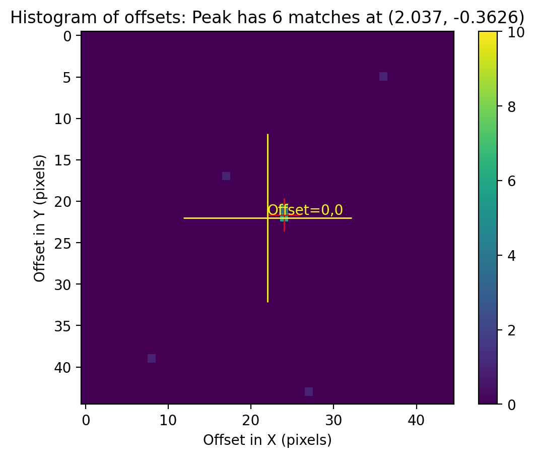
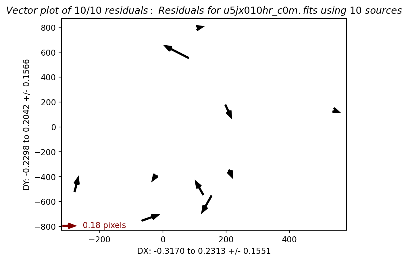
Inspect the shift file and fit residuals#
We can look at the shift file to see how well the fit did (or we could open the output png images for more information). The columns are:
Filename, X Shift [pixels], Y Shift [pixels], Rotation [degrees], Scale, X RMS [pixels], Y RMS [pixels]
Note that there is a small shift in x=1.8 pix and y=-0.4 pix and large rotation of 0.014 degrees between the two images, likely due to the large chip-sized dither. These residuals are larger than the RMS scatter of 0.15 pixels and are therefore likely to be real.
shift_flt_table = Table.read('shift_flt.txt', format='ascii.no_header',
                             names=['file', 'dx', 'dy', 'rot', 'scale', 'xrms', 'yrms'])

formats = ['.2f', '.2f', '.3f', '.5f', '.2f', '.2f']
for i, col in enumerate(shift_flt_table.colnames[1:]):
    shift_flt_table[col].format = formats[i]
shift_flt_table
| file | dx | dy | rot | scale | xrms | yrms |
|---|---|---|---|---|---|---|
| str18 | float64 | float64 | float64 | float64 | float64 | float64 |
| u5jx0108r_flt.fits | 0.00 | 0.00 | 0.000 | 1.00000 | 0.00 | 0.00 |
| u5jx010hr_flt.fits | 1.81 | -0.40 | 0.014 | 1.00001 | 0.15 | 0.15 |
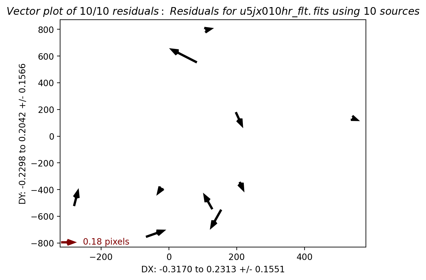
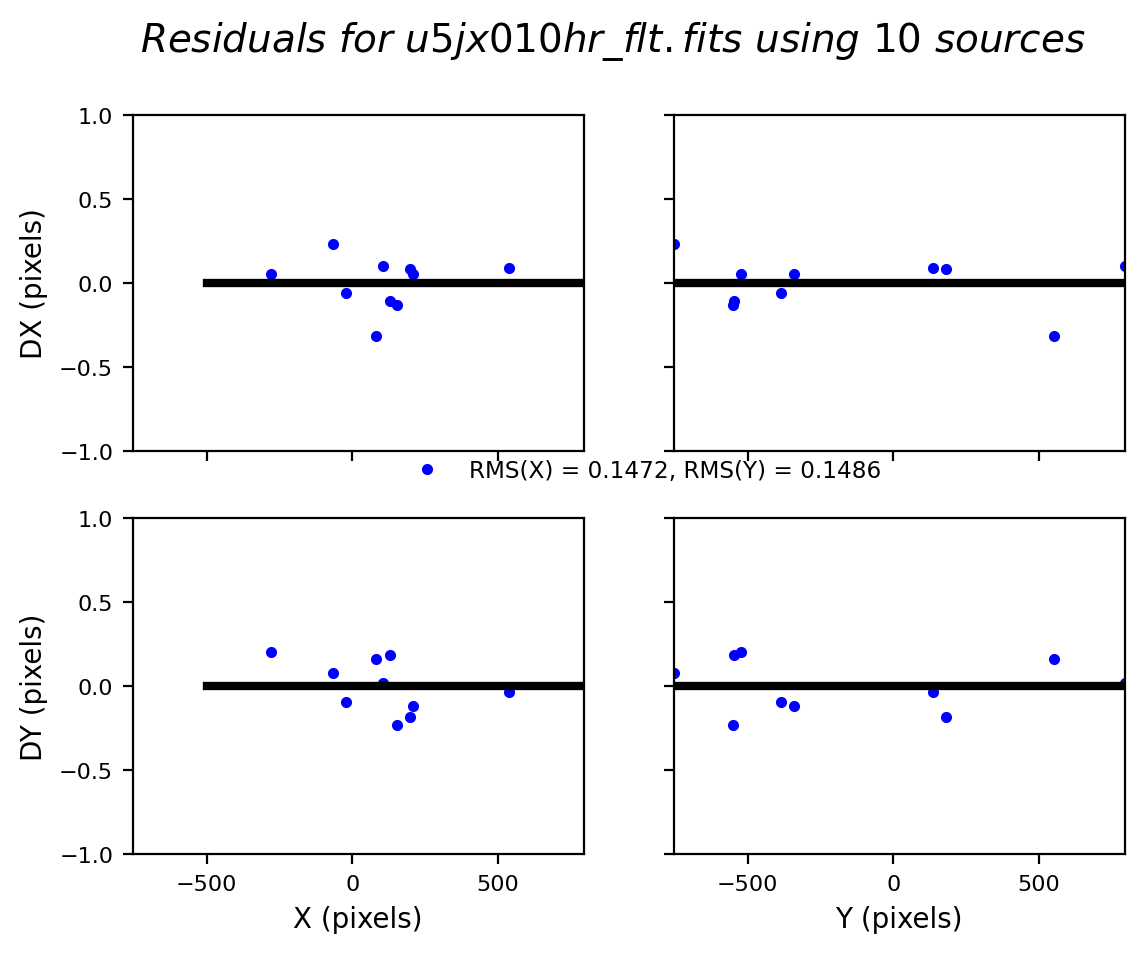
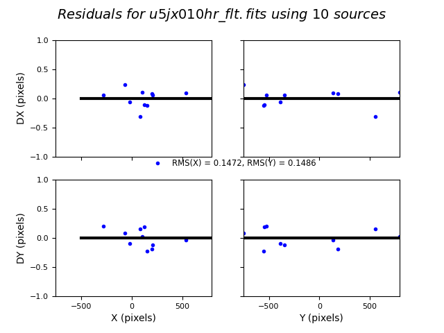
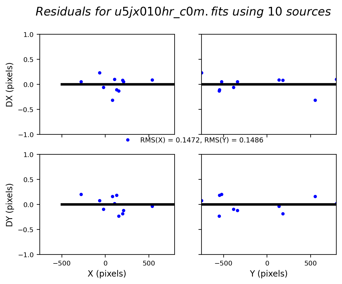
Inspect the Astrometric residual scatter plots#
Good practice includes inspecting not only the shift file residuals, but also the accompanying diagnostic plots. The residuals in the plot below are clustered around 0.0 with no obvious systematics.
Image(filename='residuals_u5jx010hr_flt.png', width=500, height=300)
Here we align the c0m files with the same parameter settings:
input_images = sorted(glob.glob('u*c0m.fits'))

tweakreg.TweakReg(input_images,
                  updatehdr=True,
                  clean=True,
                  reusename=True,
                  interactive=False,
                  conv_width=3.0,
                  threshold=200.0,
                  ylimit=1,
                  shiftfile=True,
                  outshifts='shift_c0m.txt',
                  searchrad=1,
                  tolerance=3,
                  minobj=7)

clear_output()
Finally, we compare the shift file computed from the flt and c0m files to confirm that the results are identical.
shift_c0m_table = Table.read('shift_c0m.txt', format='ascii.no_header',
                             names=['file', 'dx', 'dy', 'rot', 'scale', 'xrms', 'yrms'])

formats = ['.2f', '.2f', '.3f', '.5f', '.2f', '.2f']
for i, col in enumerate(shift_c0m_table.colnames[1:]):
    shift_c0m_table[col].format = formats[i]

shift_c0m_table
| file | dx | dy | rot | scale | xrms | yrms |
|---|---|---|---|---|---|---|
| str18 | float64 | float64 | float64 | float64 | float64 | float64 |
| u5jx0108r_c0m.fits | 0.00 | 0.00 | 0.000 | 1.00000 | 0.00 | 0.00 |
| u5jx010hr_c0m.fits | 1.81 | -0.40 | 0.014 | 1.00001 | 0.15 | 0.15 |
shift_flt_table
| file | dx | dy | rot | scale | xrms | yrms |
|---|---|---|---|---|---|---|
| str18 | float64 | float64 | float64 | float64 | float64 | float64 |
| u5jx0108r_flt.fits | 0.00 | 0.00 | 0.000 | 1.00000 | 0.00 | 0.00 |
| u5jx010hr_flt.fits | 1.81 | -0.40 | 0.014 | 1.00001 | 0.15 | 0.15 |
5. Drizzle-combine the images #
All four chips are now drizzled together. For speed in the notebook, we set the output pixel scale to that of the WF chips, but this can be reset to the PC scale if desired, to match the scale of the new drw drizzled products.
While we have turned sky subtraction off in the notebook, recommend using skymethod = ‘localmin’ and not ‘match’ for WFPC2 to avoid issues with overlapping vignetted regions along chip boundaries. See Figure 3.1.2 in the WFPC2 Instrument Handbook. For more information drizzling HST data, see the Drizzlepac Handbook and the list of commands in the readthedocs.
Users may wish turn on the sky subtraction and cosmic-ray rejection steps by setting skysub, median, blot, and driz_cr parameters to True. In that case, the recommended parameter settings for WFPC2 are driz_cr_snr='5.5 3.5', and driz_cr_scale='2.0 1.5'. For more discussion on drizzling parameters for WFPC2 when using the output scale of the WF chips, see the Prior Drizzling Example.
astrodrizzle.AstroDrizzle('u*flt.fits',
                          output='wfpc2_flt',
                          preserve=False,
                          build=False,
                          context=False,
                          skysub=False,
                          driz_sep_wcs=True,
                          driz_sep_scale=0.0996,
                          driz_sep_bits='8,1024',
                          driz_sep_fillval=-1,
                          median=False,
                          blot=False,
                          driz_cr=False,
                          final_fillval=None,
                          final_bits='8,1024',
                          final_wcs=True,
                          final_scale=0.0996)
clear_output()
astrodrizzle.AstroDrizzle('u*c0m.fits',
                          output='wfpc2_c0m',
                          preserve=False,
                          build=False,
                          context=False,
                          static=True,
                          skysub=False,
                          driz_sep_wcs=True,
                          driz_sep_refimage='u5jx010hr_single_sci.fits',
                          driz_sep_bits='8,1024',
                          driz_sep_fillval=-1,
                          median=False,
                          blot=False,
                          driz_cr=False,
                          final_fillval=None,
                          final_bits='8,1024',
                          final_wcs=True,
                          final_scale=0.0996,
                          final_refimage='wfpc2_flt_drw_sci.fits')
clear_output()
Clean up unnecessary mask files.
fits_files = glob.glob('*ask.fits')
for f in fits_files:
    base_name = os.path.basename(f)
    if os.path.isfile(base_name):
        os.remove(base_name)
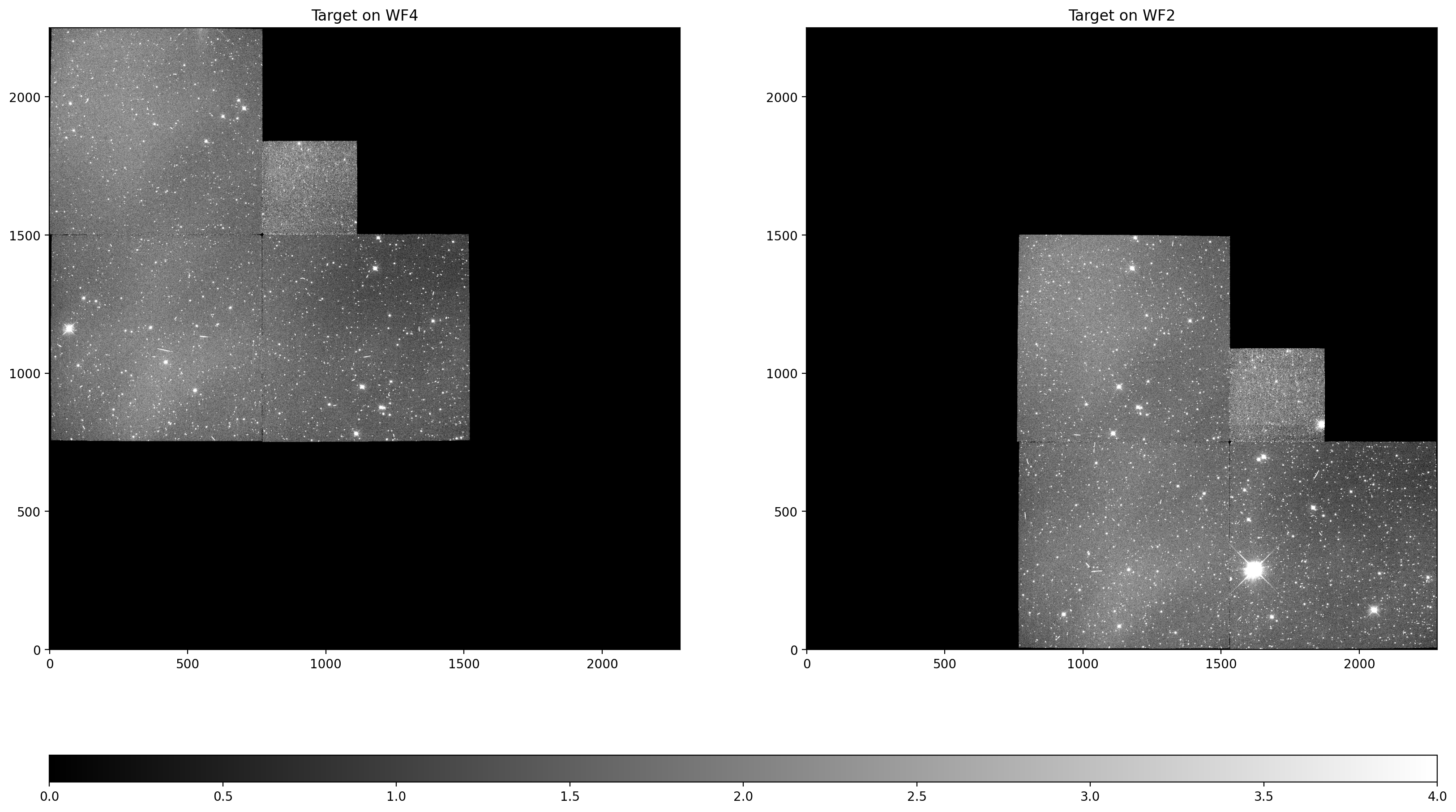
Inspect the single drizzled output frames derived from the dithered flt inputs#
Here we compare the single drizzled frames. Note that WF4 and WF2 overlap in the footprint on the sky.
drz1_single = fits.getdata('u5jx010hr_single_sci.fits')
drz2_single = fits.getdata('u5jx0108r_single_sci.fits')

fig, (ax1, ax2) = plt.subplots(ncols=2, figsize=(20, 10))
im1 = ax1.imshow(drz1_single, cmap='gray', vmin=0, vmax=4, origin='lower')
ax1.set_title('Target on WF4')
im2 = ax2.imshow(drz2_single, cmap='gray', vmin=0, vmax=4, origin='lower')
ax2.set_title('Target on WF2')

x1 = ax1.get_position().get_points().flatten()[0]
x2 = ax2.get_position().get_points().flatten()[2] - x1
ax_cbar = fig.add_axes([x1, 0, x2, 0.03])
plt.colorbar(im1, cax=ax_cbar, orientation='horizontal')
plt.show()
Inspect the single drizzled output frames derived from the dithered c0m inputs#
drz1_c0m_single = fits.getdata('u5jx010hr_c0m_single_sci.fits')
drz2_c0m_single = fits.getdata('u5jx0108r_c0m_single_sci.fits')

fig, (ax1, ax2) = plt.subplots(ncols=2, figsize=(20, 10))
im1 = ax1.imshow(drz1_single, cmap='gray', vmin=0, vmax=4, origin='lower')
ax1.set_title('Target on WF4')
im2 = ax2.imshow(drz2_single, cmap='gray', vmin=0, vmax=4, origin='lower')
ax2.set_title('Target on WF2')

x1 = ax1.get_position().get_points().flatten()[0]
x2 = ax2.get_position().get_points().flatten()[2] - x1
ax_cbar = fig.add_axes([x1, 0, x2, 0.03])
plt.colorbar(im1, cax=ax_cbar, orientation='horizontal')
plt.show()
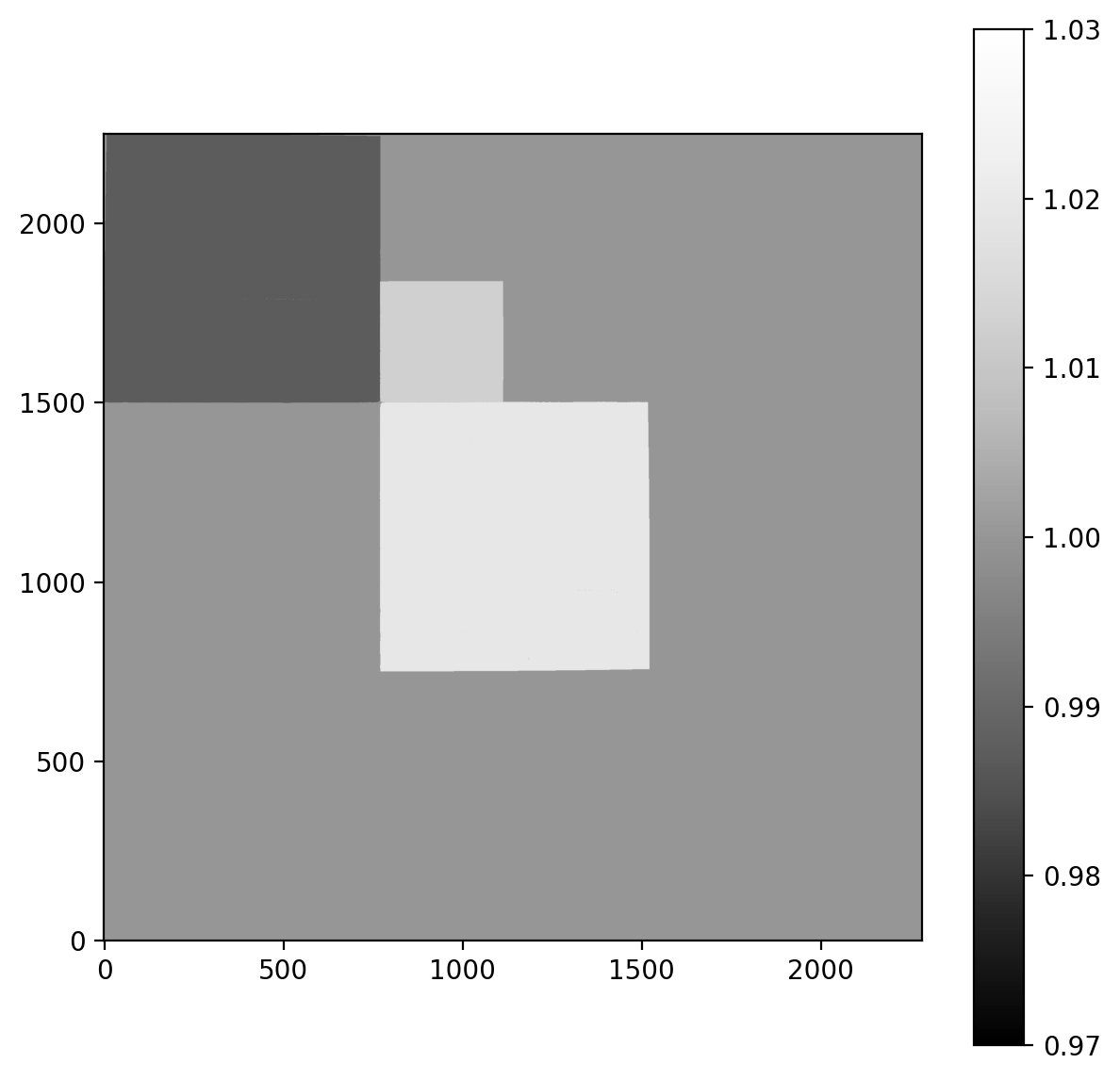
Inspect the ratio of the two drizzled images to see changes due to photometric normalization#
ratio_flt_c0m = drz1_single/drz1_c0m_single
fig = plt.figure(figsize=(7, 7))
img_ratio = plt.imshow(ratio_flt_c0m, vmin=0.97, vmax=1.03, cmap='Greys_r', origin='lower')
plt.colorbar(img_ratio, orientation='vertical')
plt.show()
Compare the combined drizzled image and the weight image.#
flt_drw_sci = fits.getdata('wfpc2_flt_drw_sci.fits')
flt_drw_wht = fits.getdata('wfpc2_flt_drw_wht.fits')
fig, (ax1, ax2) = plt.subplots(ncols=2, figsize=(20, 10))
im1 = ax1.imshow(flt_drw_sci, cmap='gray', vmin=0, vmax=0.5, origin='lower')
ax1.set_title('SCI')
im2 = ax2.imshow(flt_drw_wht, cmap='gray', vmin=0, vmax=50, origin='lower')
ax2.set_title('WHT')
x1 = ax1.get_position().get_points().flatten()[0]
x2 = ax2.get_position().get_points().flatten()[2] - x1
ax_cbar = fig.add_axes([x1, 0, x2, 0.03])
plt.colorbar(im1, cax=ax_cbar, orientation='horizontal')
plt.show()
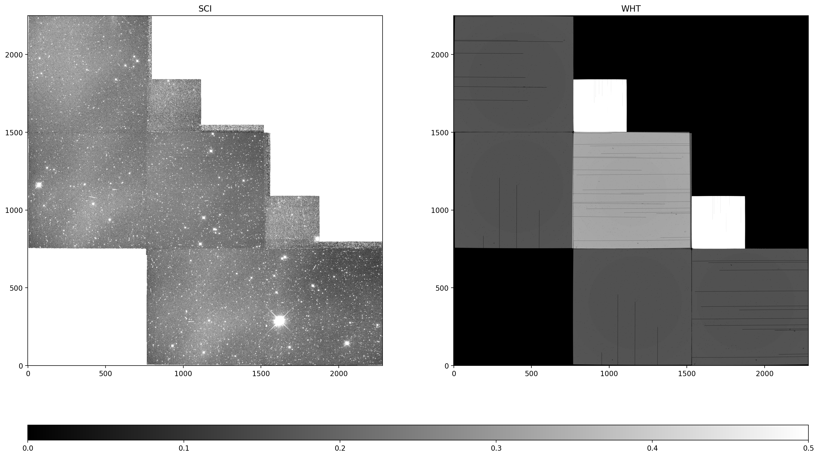
Note the Planetary Chip (PC) has ~4x WHT because the native pixel scale is ~2x smaller.
scale_ratio = 0.0996/0.0455
area_ratio = scale_ratio**2
print('')
print('PIXEL SCALE RATIO: WF/PC = (0.0996/0.0455) =    ', scale_ratio)
print('PIXEL AREA  RATIO: WF/PC = (0.0996/0.0455)**2 = ', area_ratio)
PIXEL SCALE RATIO: WF/PC = (0.0996/0.0455) =     2.189010989010989
PIXEL AREA  RATIO: WF/PC = (0.0996/0.0455)**2 =  4.7917691100108675
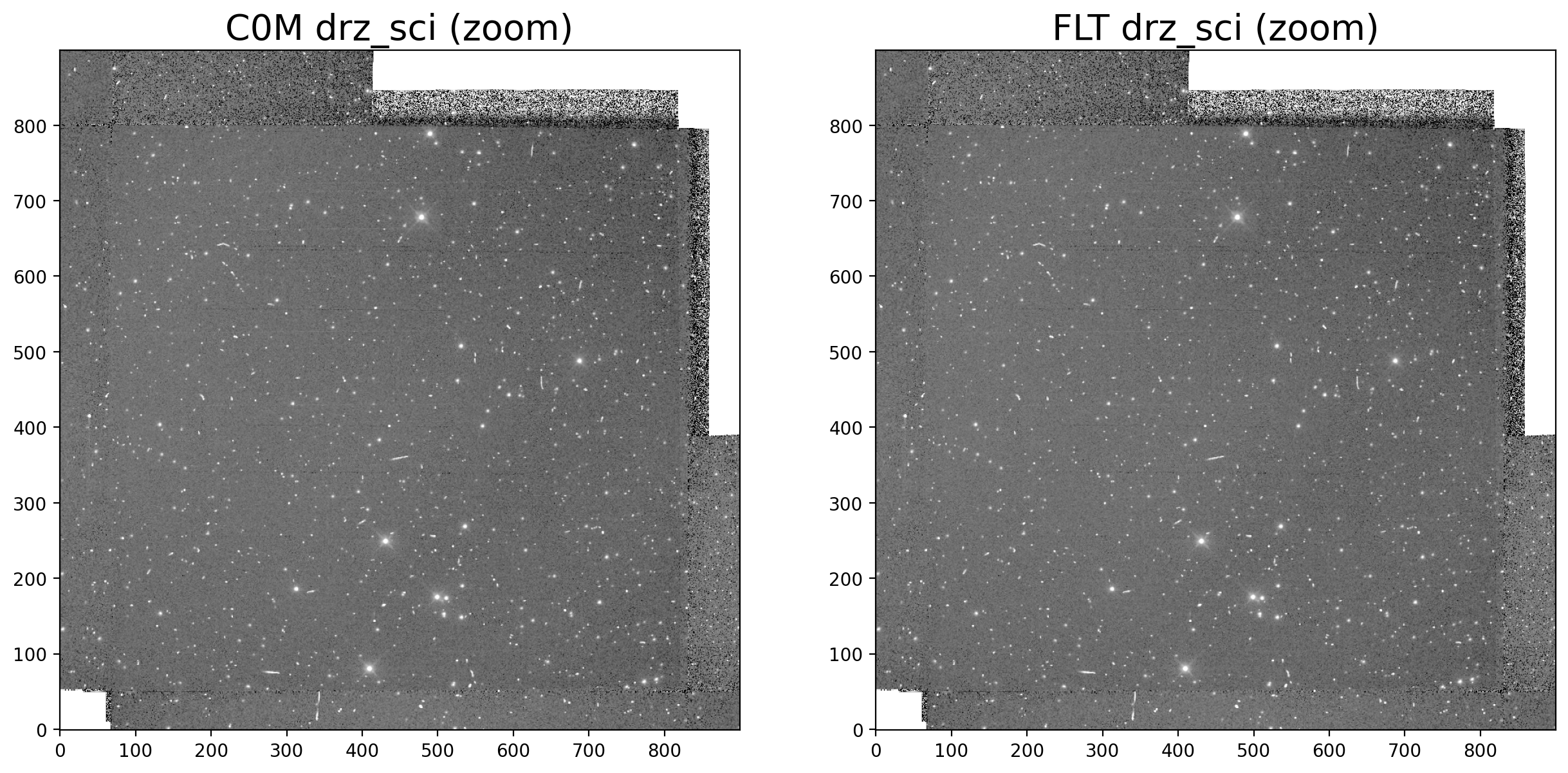
Next, we compare the two drizzled images, zooming in to highlight where the two chips overlap. Note that the one on the right has a slightly more uniform background across the field of view. Finally, we then identify three isolated stars for photometry.
c0m_drw_sci = fits.getdata('wfpc2_c0m_drw_sci.fits')
flt_drw_sci = fits.getdata('wfpc2_flt_drw_sci.fits')

im1 = c0m_drw_sci[700:1600, 700:1600]
im2 = flt_drw_sci[700:1600, 700:1600]

fig, ax = plt.subplots(1, 2, figsize=(15, 10))
norm1 = ImageNormalize(im1, vmin=0.1, vmax=8, stretch=LogStretch())
ax[0].imshow(im1, norm=norm1, cmap='gray', origin='lower')
ax[1].imshow(im2, norm=norm1, cmap='gray', origin='lower')
ax[0].set_title('C0M drz_sci (zoom)', fontsize=20)
ax[1].set_title('FLT drz_sci (zoom)', fontsize=20)
plt.show()
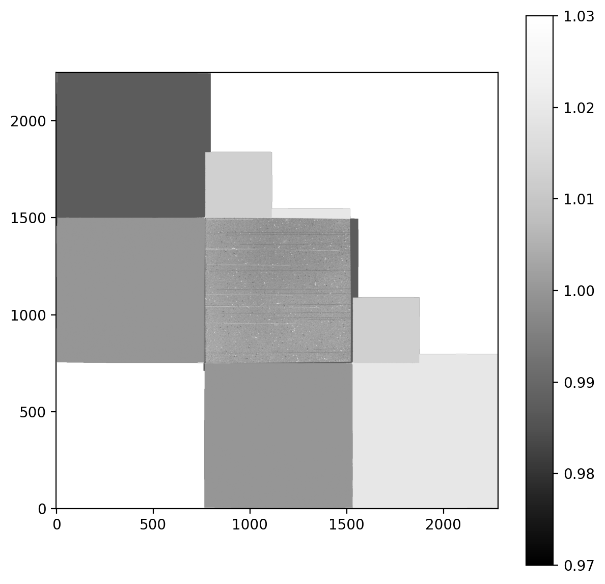
Plot the ratio of the combined drizzled images from FLT and C0M#
ratio_drw = flt_drw_sci/c0m_drw_sci
fig = plt.figure(figsize=(7, 7))
img_ratio = plt.imshow(ratio_drw, vmin=0.97, vmax=1.03, cmap='Greys_r', origin='lower')
plt.colorbar(img_ratio, orientation='vertical')
plt.show()
Perform aperture photometry on three stars in the WF2, WF4 overlap region#
Here we perform aperture photometry in a radius of 5 pixels to show the change in count rates in each drizzle-combined image.
positions = [(1180, 1381), (1388, 1190), (1232, 1210)]    # Coords are (Y+1, X+1)
aperture = CircularAperture(positions, r=5)
annulus_aperture = CircularAnnulus(positions, r_in=10, r_out=15)

print('Aperture radius:', aperture)
print('Annulus:', annulus_aperture)
Aperture radius: Aperture: CircularAperture
positions: [[1180., 1381.],
            [1388., 1190.],
            [1232., 1210.]]
r: 5.0
Annulus: Aperture: CircularAnnulus
positions: [[1180., 1381.],
            [1388., 1190.],
            [1232., 1210.]]
r_in: 10.0
r_out: 15.0
data = fits.getdata('wfpc2_flt_drw_sci.fits')
aperstats = ApertureStats(data, annulus_aperture)
bkg_mean = aperstats.mean

phot_table = aperture_photometry(data, aperture)

for col in phot_table.colnames:
    phot_table[col].info.format = '%.8g'  # for consistent table output

print('drz_flt_combined: "wfpc2_flt_drw_sci.fits"')
print('     SKY values :', bkg_mean)
print('---------------------------------')
print(phot_table)
drz_flt_combined: "wfpc2_flt_drw_sci.fits"
     SKY values : [0.31061331 0.25361143 0.25064782]
---------------------------------
 id xcenter ycenter aperture_sum
--- ------- ------- ------------
  1    1180    1381    1139.9086
  2    1388    1190    484.00455
  3    1232    1210    210.30805
data = fits.getdata('wfpc2_c0m_drw_sci.fits')
aperstats = ApertureStats(data, annulus_aperture)
bkg_mean = aperstats.mean

phot_table = aperture_photometry(data, aperture)

for col in phot_table.colnames:
    phot_table[col].info.format = '%.8g'  # for consistent table output

print('drz_c0m_combined: "wfpc2_c0m_drw_sci.fits"')
print('     SKY values :', bkg_mean)
print('---------------------------------')
print(phot_table)
drz_c0m_combined: "wfpc2_c0m_drw_sci.fits"
     SKY values : [0.31046403 0.25329725 0.25064313]
---------------------------------
 id xcenter ycenter aperture_sum
--- ------- ------- ------------
  1    1180    1381    1136.0271
  2    1388    1190    482.57234
  3    1232    1210    209.71238
While the total change in photometry is only a few DN/sec, properly accounting for the relative gain across chips is necessary to achieve the best possible photometric precision. As we’ve demonstrated in this notebook, this is accomplished by using the new flt style files, or running photeq on the older c0m style files.
Conclusions #
MAST now include new WFPC2 flt.fits data products to replace the old c0m.fits, c1m.fits files. The new products include a new flux normalization between chips so that only a single zeropoint (inverse sensitivity, PHOTFLAM value) is needed for all chips. This allows for different chips to be drizzled together, for example, when combining images at multiple orientations.
About this Notebook#
Created: 14 Dec 2018;     M. Cara
Updated: 16 Nov 2023;     K. Huynh & J. Mack
Updated: 10 Dec 2024;     J. Mack & M. Revalski
Source: spacetelescope/hst_notebooks
Additional Resources#
Below are some additional resources that may be helpful. Please send any questions to the HST Help Desk.
Software Citations#
If you use Python packages such as astropy, astroquery, drizzlepac, matplotlib, or numpy for published research, please cite the authors. Follow the links below for more information about citing various packages:
