Optimizing the Image Sampling#
Table of Contents#
1. Retrieve Observations
2. Check image header data
2.1 Inspect useful keywords
2.2 Inspect the dither pattern
2.3 Inspect the MAST alignment
2.4 Reset the WCS solution
3. Drizzling
4. Inspecting the Results
5. Optimizing the final_pixfrac parameter
6. Final Thoughts
Introduction#
This example was written to help users better understand the subtleties in improving image sampling for dithered data. One of the powers of the drizzling algorithm is that, given properly dithered images, it can restore much of the information lost due to undersampled images (Fruchter and Hook, 2002).
This work is based on ISR ACS 2015-01, which contains a more detailed discussion than presented here.
In practice, this requires the use of Astrodrizzle task within the Drizzlepac package. This example will:
- Run astrodrizzle several times using different parameter settings for 'final_pixfrac' and 'final_scale'
- Compare and evaluate results of using different 'final_pixfrac' and 'final_scale' values
Import packages#
The following Python packages are required to run the Jupyter Notebook:
os - change and make directories
glob - gather lists of filenames
shutil - remove directories and files
numpy - math and array functions
matplotlib - make figures and graphics
astropy - file handling, tables, units, WCS, statistics
astroquery - download data and query databases
drizzlepac - align and combine HST images
[stwcs] - tools for manipulating headerlets
import os
import glob
import shutil

import numpy as np
import matplotlib.pyplot as plt
from collections import defaultdict
from IPython.display import clear_output

from astropy.io import fits
from astroquery.mast import Observations
from astropy.visualization import LogStretch, ImageNormalize, LinearStretch
from astropy import wcs
from astropy.table import Table

from stwcs.wcsutil import headerlet
import drizzlepac

%matplotlib inline
%config InlineBackend.figure_format = 'retina' # Greatly improves the resolution of figures rendered in notebooks.

# Set the locations of reference files.  and retrieve the MDRIZTAB recommended drizzle parameters.
os.environ['CRDS_SERVER_URL'] = 'https://hst-crds.stsci.edu'
os.environ['CRDS_SERVER'] = 'https://hst-crds.stsci.edu'
os.environ['CRDS_PATH'] = './crds_cache'
os.environ['iref'] = './crds_cache/references/hst/wfc3/'
os.environ['jref'] = './crds_cache/references/hst/acs/'
1. Download the Observations with astroquery#
MAST queries may be done using `query_criteria`, where we specify:
–> obs_id, proposal_id, and filters
MAST data products may be downloaded by using download_products, where we specify:
–> products = calibrated (FLT, FLC) or drizzled (DRZ, DRC) files
–> type = standard products (CALxxx) or advanced products (HAP-SVM)
Observations of the spiral galaxy NGC 3370 (Program 11570) were acquired using the WFC3/IR F160W imaging filter. The WFC3-IR-DITHERBOX-MIN dither pattern designed to provide optimal sampling of the PSF was used.
For this example, the four calibrated FLT exposures from visit 19 will be downloaded and moved to the local directory.
        ib1f19l6q_flt.fits
        ib1f19l7q_flt.fits
        ib1f19l8q_flt.fits
        ib1f19l9q_flt.fits
obs_ids = ['ib1f19010']

obsTable = Observations.query_criteria(obs_id=obs_ids)
products = Observations.get_product_list(obsTable)

data_prod = ['FLT']                                 # ['FLC','FLT','DRC','DRZ']
data_type = ['CALWF3']                              # ['CALACS','CALWF3','CALWP2','HAP-SVM']

Observations.download_products(products, productSubGroupDescription=data_prod, project=data_type, cache=True)
Downloading URL https://mast.stsci.edu/api/v0.1/Download/file?uri=mast:HST/product/ib1f19l6q_flt.fits to ./mastDownload/HST/ib1f19l6q/ib1f19l6q_flt.fits ...
[Done]
Downloading URL https://mast.stsci.edu/api/v0.1/Download/file?uri=mast:HST/product/ib1f19l7q_flt.fits to ./mastDownload/HST/ib1f19l7q/ib1f19l7q_flt.fits ...
[Done]
Downloading URL https://mast.stsci.edu/api/v0.1/Download/file?uri=mast:HST/product/ib1f19l9q_flt.fits to ./mastDownload/HST/ib1f19l9q/ib1f19l9q_flt.fits ...
[Done]
Downloading URL https://mast.stsci.edu/api/v0.1/Download/file?uri=mast:HST/product/ib1f19laq_flt.fits to ./mastDownload/HST/ib1f19laq/ib1f19laq_flt.fits ...
[Done]
| Local Path | Status | Message | URL |
|---|---|---|---|
| str47 | str8 | object | object |
| ./mastDownload/HST/ib1f19l6q/ib1f19l6q_flt.fits | COMPLETE | None | None |
| ./mastDownload/HST/ib1f19l7q/ib1f19l7q_flt.fits | COMPLETE | None | None |
| ./mastDownload/HST/ib1f19l9q/ib1f19l9q_flt.fits | COMPLETE | None | None |
| ./mastDownload/HST/ib1f19laq/ib1f19laq_flt.fits | COMPLETE | None | None |
# Move to the files to the local working directory

for flt in glob.glob('./mastDownload/HST/*/*fl?.fits'):
    flt_name = os.path.split(flt)[-1]
    os.rename(flt, flt_name)
shutil.rmtree('mastDownload/')
2. Check image header data#
Here we will look at important keywords in the image headers to summarize the observation strategy.
2.1 Inspect useful keywords#
flt_files = sorted(glob.glob('*fl?.fits'))

data = []
keywords_ext0 = ["ROOTNAME", "ASN_ID", "TARGNAME", "DETECTOR", "FILTER", "EXPTIME",
                 "RA_TARG", "DEC_TARG", "POSTARG1", "POSTARG2", "DATE-OBS"]
keywords_ext1 = ["ORIENTAT"]

for flt_file in flt_files:
    path_data = []
    for keyword in keywords_ext0:
        path_data.append(fits.getval(flt_file, keyword, ext=0))
    for keyword in keywords_ext1:
        path_data.append(fits.getval(flt_file, keyword, ext=1))
    data.append(path_data)

keywords = keywords_ext0 + keywords_ext1
table = Table(np.array(data), names=keywords, dtype=['str', 'str', 'str', 'str', 'str', 'f8', 'f8', 'f8', 'f8', 'f8', 'str', 'f8'])
table['EXPTIME'].format = '7.1f'
table['RA_TARG'].format = table['DEC_TARG'].format = '7.4f'
table['POSTARG1'].format = table['POSTARG2'].format = '7.3f'
table['ORIENTAT'].format = '7.2f'
table
| ROOTNAME | ASN_ID | TARGNAME | DETECTOR | FILTER | EXPTIME | RA_TARG | DEC_TARG | POSTARG1 | POSTARG2 | DATE-OBS | ORIENTAT |
|---|---|---|---|---|---|---|---|---|---|---|---|
| str32 | str32 | str32 | str32 | str32 | float64 | float64 | float64 | float64 | float64 | str32 | float64 |
| ib1f19l6q | IB1F19010 | NGC-3370 | IR | F160W | 502.9 | 161.7694 | 17.2732 | 0.000 | 0.000 | 2010-04-04 | 5.63 |
| ib1f19l7q | IB1F19010 | NGC-3370 | IR | F160W | 502.9 | 161.7694 | 17.2732 | 0.542 | 0.182 | 2010-04-04 | 5.63 |
| ib1f19l9q | IB1F19010 | NGC-3370 | IR | F160W | 502.9 | 161.7694 | 17.2732 | 0.339 | 0.485 | 2010-04-04 | 5.63 |
| ib1f19laq | IB1F19010 | NGC-3370 | IR | F160W | 502.9 | 161.7694 | 17.2732 | -0.203 | 0.303 | 2010-04-04 | 5.63 |
2.2 Inspect the dither pattern#
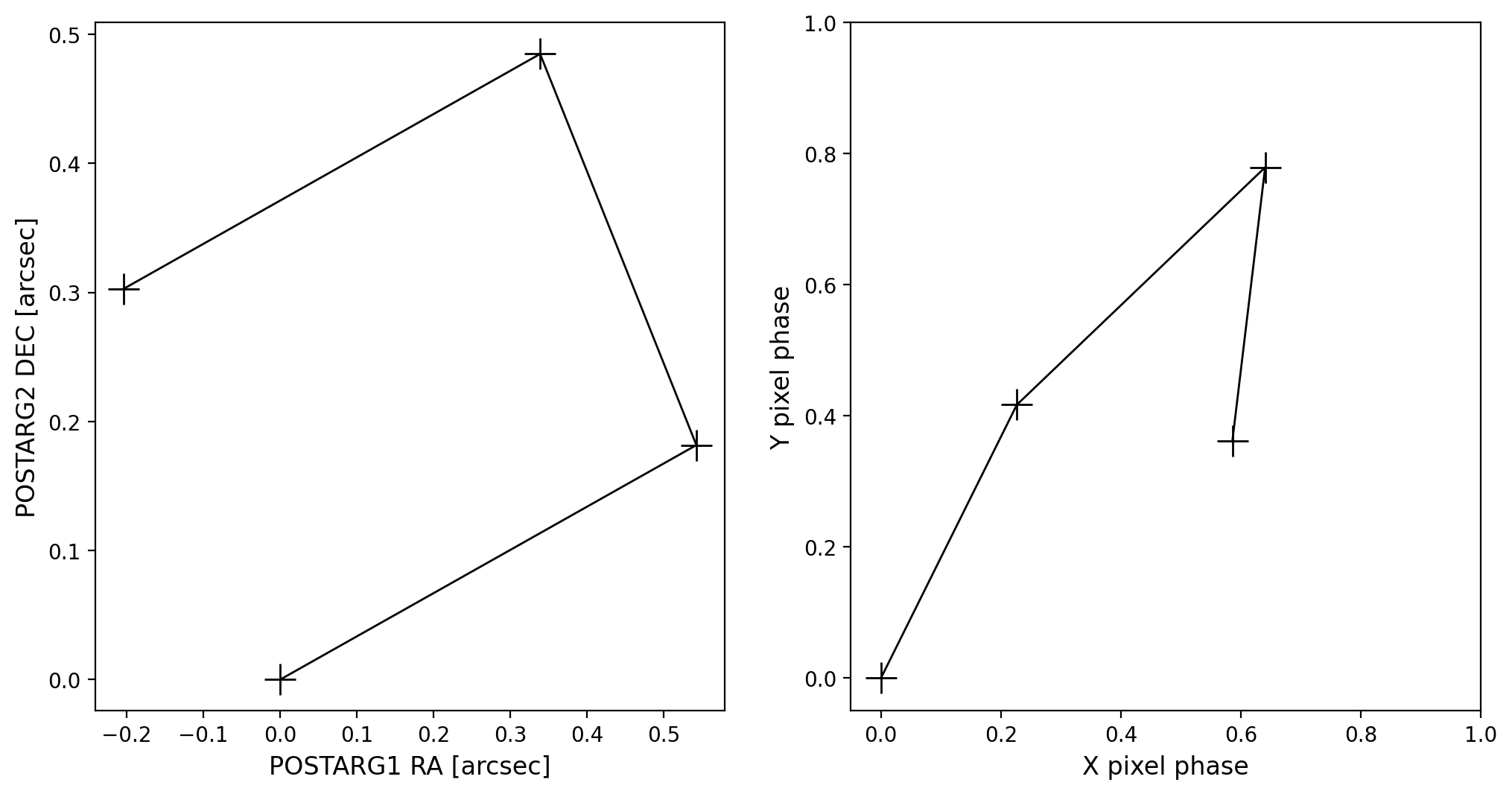
For the drizzle algorithm to work optimally, observations need to be dithered so that the PSF is appropriately sampled. The code below creates plots to show the dithering of each of the images in the association. The plot on the left shows how the images were dithered on the sky (the POSTARG). The plot on the right shows how the offsets translate to pixel phase (e.g. subpixel position).
plate_scale = fits.getval(flt_files[0], 'idcscale', ext=1)
print('Detector Plate scale: {:>6.4f}'.format(plate_scale))
postarg1 = np.empty(len(flt_files), dtype=np.float16)
postarg2 = np.empty(len(flt_files), dtype=np.float16)
x_phase = np.empty(len(flt_files), dtype=np.float16)
y_phase = np.empty(len(flt_files), dtype=np.float16)

for i, im in enumerate(flt_files):
    with fits.open(im) as hdu:
        postarg1[i] = hdu[0].header['postarg1']
        postarg2[i] = hdu[0].header['postarg2']
        x_phase[i] = abs(np.modf(postarg1[i] / plate_scale)[0])
        y_phase[i] = abs(np.modf(postarg2[i] / plate_scale)[0])

fig, ax = plt.subplots(1, 2, figsize=(12, 6))

ax[0].plot(postarg1, postarg2, 'k+-', ms=15, lw=1)
ax[0].set_xlabel('POSTARG1 RA [arcsec]', fontsize='large')
ax[0].set_ylabel('POSTARG2 DEC [arcsec]', fontsize='large')

ax[1].plot(x_phase, y_phase, 'k+-', ms=15, lw=1)
ax[1].set_xlim(-0.05, 1)
ax[1].set_ylim(-0.05, 1)
ax[1].set_xlabel('X pixel phase', fontsize='large')
ax[1].set_ylabel('Y pixel phase', fontsize='large')
2.3 Inspect the MAST alignment#
Check the active WCS solution in the FITS image header. If the image is aligned to a catalog, list the number of matches and the fit RMS in milli-arcseconds and in pixels.
ext_0_kws = ['DETECTOR', 'EXPTIME']
ext_1_kws = ['WCSNAME', 'NMATCHES', 'RMS_RA', 'RMS_DEC']

det_scale = {'IR': 0.1283, 'UVIS': 0.0396, 'WFC': 0.05}                    # plate scale (arcsec/pixel)

format_dict = {}
col_dict = defaultdict(list)

for f in flt_files:
    col_dict['filename'].append(f)
    hdr0 = fits.getheader(f, 0)
    hdr1 = fits.getheader(f, 1)

    for kw in ext_0_kws:                                                # extension 0 keywords
        col_dict[kw].append(hdr0[kw])
    for kw in ext_1_kws:                                                # extension 1 keywords
        if 'RMS' in kw:
            val = np.around(hdr1[kw], 1)
        else:
            val = hdr1[kw]
        col_dict[kw].append(val)

    for kw in ['RMS_RA', 'RMS_DEC']:
        val = np.round(hdr1[kw]/1000./det_scale[hdr0['DETECTOR']], 2)  # convert RMS from mas to pixels
        col_dict[f'{kw}_pix'].append(val)

wcstable = Table(col_dict)
wcstable
| filename | DETECTOR | EXPTIME | WCSNAME | NMATCHES | RMS_RA | RMS_DEC | RMS_RA_pix | RMS_DEC_pix |
|---|---|---|---|---|---|---|---|---|
| str18 | str2 | float64 | str28 | int64 | float64 | float64 | float64 | float64 |
| ib1f19l6q_flt.fits | IR | 502.936462 | IDC_w3m18525i-FIT_REL_GSC242 | 26 | 87.7 | 98.4 | 0.68 | 0.77 |
| ib1f19l7q_flt.fits | IR | 502.936462 | IDC_w3m18525i-FIT_REL_GSC242 | 26 | 87.7 | 98.4 | 0.68 | 0.77 |
| ib1f19l9q_flt.fits | IR | 502.936462 | IDC_w3m18525i-FIT_REL_GSC242 | 26 | 87.7 | 98.4 | 0.68 | 0.77 |
| ib1f19laq_flt.fits | IR | 502.936462 | IDC_w3m18525i-FIT_REL_GSC242 | 26 | 87.7 | 98.4 | 0.68 | 0.77 |
Here we see that the four FLC images have a “FIT_REL_GSC242” WCS solution, which means they were aligned as a set to the reference catalog ‘GSC v2.4.2’ using the drizzled-combined (DRC) image, and that WCS was propogated back to the original FLCs. This is reflected in the fact that the number of matches and fit rms values are the same for each FLC frame.
Note that the alignment was based on 26 matches to the GSC v2.4.2 catalog. This means that the target did not successfully align to the Gaia eDR3 solution since there are very few stars in the frame.
We can various functions within the headerlet of the stwcs package to find, list, and ultimately update the WCS solutions in an image. Let’s make a list of the images and then print out all the WCS solutions in the first image in the list.
wcsnames = headerlet.get_headerlet_kw_names(flt_files[0], kw='WCSNAME')
wcsnames
['OPUS',
 'IDC_w3m18525i',
 'IDC_w3m18525i-GSC240',
 'IDC_w3m18525i-HSC30',
 'IDC_w3m18525i',
 'IDC_w3m18525i-FIT_REL_GSC242']
For more details on the WCS naming convention, see DrizzlePac readthedocs
For more discussion on absolute astrometry, see Section 4.5 in the DrizzlePac Handbook
2.4 Reset the WCS solution#
Next, we find the index of the WCS solution we want to use, and then apply that solution to each of the science images. Because the program was designed to have precise dithers, we reset the WCS to the “a priori” (distortion-only) solution to preserve relative alignment and get the sharpest PSFs when drizzling the images together.
In this example, the “a priori” solution is named IDC_w3m18525i-GSC240, in which the coordinates of the guide stars were corrected to the coordinates reported in GAIA DR1, with no additional catalog fitting.
Here we first grab the index of list element with value ‘IDC_w3m18525i-GSC240’. The index in this list + 1 is the same as the EXTVER of the corresponding HDRLET. We need to add 1 because lists are 0-indexed, while EXTVER’s are 1 indexed.
for flt_file in flt_files:

    chosen_ext = wcsnames.index('IDC_w3m18525i-GSC240')+1
    headerlet.restore_from_headerlet(flt_file, hdrext=('HDRLET', chosen_ext), archive=False, force=False)
    print(f'Image: {flt_file} WCSNAME: {fits.getval(flt_file, "wcsname", ext=1)}')
Image: ib1f19l6q_flt.fits WCSNAME: IDC_w3m18525i-GSC240
Image: ib1f19l7q_flt.fits WCSNAME: IDC_w3m18525i-GSC240
Image: ib1f19l9q_flt.fits WCSNAME: IDC_w3m18525i-GSC240
Image: ib1f19laq_flt.fits WCSNAME: IDC_w3m18525i-GSC240
Since the relative alignment of the individual FLC frames is preserved with the ‘a priori’ solution, we do not need run TweakReg before drizzling the images.
3. Drizzling#
Before drizzling can be performed, a plate scale for the output image should be chosen. This will usually be dictated by the science needs. In theory, critical sampling of a PSF occurs with 2.355 pixels. The FWHM of the WFC3/IR detector at 1600 nm is ~0.151” (Table 7.5 of WFC Instrument Handbook).
Using these values, we select a plate scale of 0.065”/pix for the drizzled output frame, approximately half of the native plate scale (0.1283”/pix).
The mechanism by which the drizzle algorithm improves sampling in the output image is by shrinking the input pixels before adding them to the output pixel grid (see Figure 2 in Fruchter and Hook (2002)). In practice this process is controlled in the AstroDrizzle package by adjusting the final_pixfrac parameter, which is the fractional size of the pixel to be used.
Below AstroDrizzle is called twice. The first time, no changes are made to the plate scale or the size of the drop. In the second call, the plate scale and pixfrac are reduced.
Next, we get some recommended values for drizzling from the MDRIZTAB reference file. The parameters in this file are different for each detector and are based on the number of input frames. These are a good starting point for drizzling and may be adjusted accordingly.
To see the full list of AstroDrizzle parameters, consult the DrizzlePac readthedocs page.
mdz = fits.getval(flt_files[0], 'MDRIZTAB', ext=0).split('$')[1]
print('Searching for the MDRIZTAB file:', mdz)
!crds sync --hst --files {mdz} --output-dir {os.environ['iref']}
Searching for the MDRIZTAB file: 3562021pi_mdz.fits
CRDS - INFO -  Symbolic context 'hst-latest' resolves to 'hst_1298.pmap'
CRDS - INFO -  Reorganizing 0 references from 'instrument' to 'flat'
CRDS - INFO -  Reorganizing from 'instrument' to 'flat' cache,  removing instrument directories.
CRDS - INFO -  Syncing explicitly listed files.
CRDS - INFO -  0 errors
CRDS - INFO -  0 warnings
CRDS - INFO -  4 infos
def get_vals_from_mdriztab(input_images, kw_list=['driz_sep_bits',
                                                  'combine_type',
                                                  'driz_cr_snr',
                                                  'driz_cr_scale',
                                                  'final_bits']):

    '''Get only selected parameters from. the MDRIZTAB'''
    mdriz_dict = drizzlepac.processInput.getMdriztabPars(input_images)

    requested_params = {}

    print('Outputting the following parameters:')
    for k in kw_list:
        requested_params[k] = mdriz_dict[k]
        print(k, mdriz_dict[k])

    return requested_params
selected_params = get_vals_from_mdriztab(flt_files)
- MDRIZTAB: AstroDrizzle parameters read from row 3.
Outputting the following parameters:
driz_sep_bits 528
combine_type median
driz_cr_snr 5.0 4.0
driz_cr_scale 3.0 2.4
final_bits 528
In this example, we have turned off the four AstroDrizzle steps used for performing CR-rejection. For WFC3/IR frames this is done in the up-the-ramp fitting in calwf3. If desired, the CR-rejection may be turned on if the user wishes to further the flagging of bad pixels.
drizzlepac.astrodrizzle.AstroDrizzle(flt_files,
                                     output='f160w_noopt',
                                     context=False, build=True, preserve=False,
                                     **selected_params,
                                     skymethod='match',
                                     driz_separate=False, median=False, blot=False, driz_cr=False, # CR-rej off
                                     final_wcs=True,
                                     final_rot=0.,
                                     final_scale=None)

drizzlepac.astrodrizzle.AstroDrizzle(flt_files,
                                     output='f160w_opt',
                                     context=False, build=True, preserve=False,
                                     **selected_params,
                                     skymethod='match',
                                     driz_separate=False, median=False, blot=False, driz_cr=False, # CR-rej off
                                     final_wcs=True,
                                     final_rot=0.,
                                     final_scale=0.065,
                                     final_pixfrac=0.8)

clear_output()
4. Inspecting the Results#
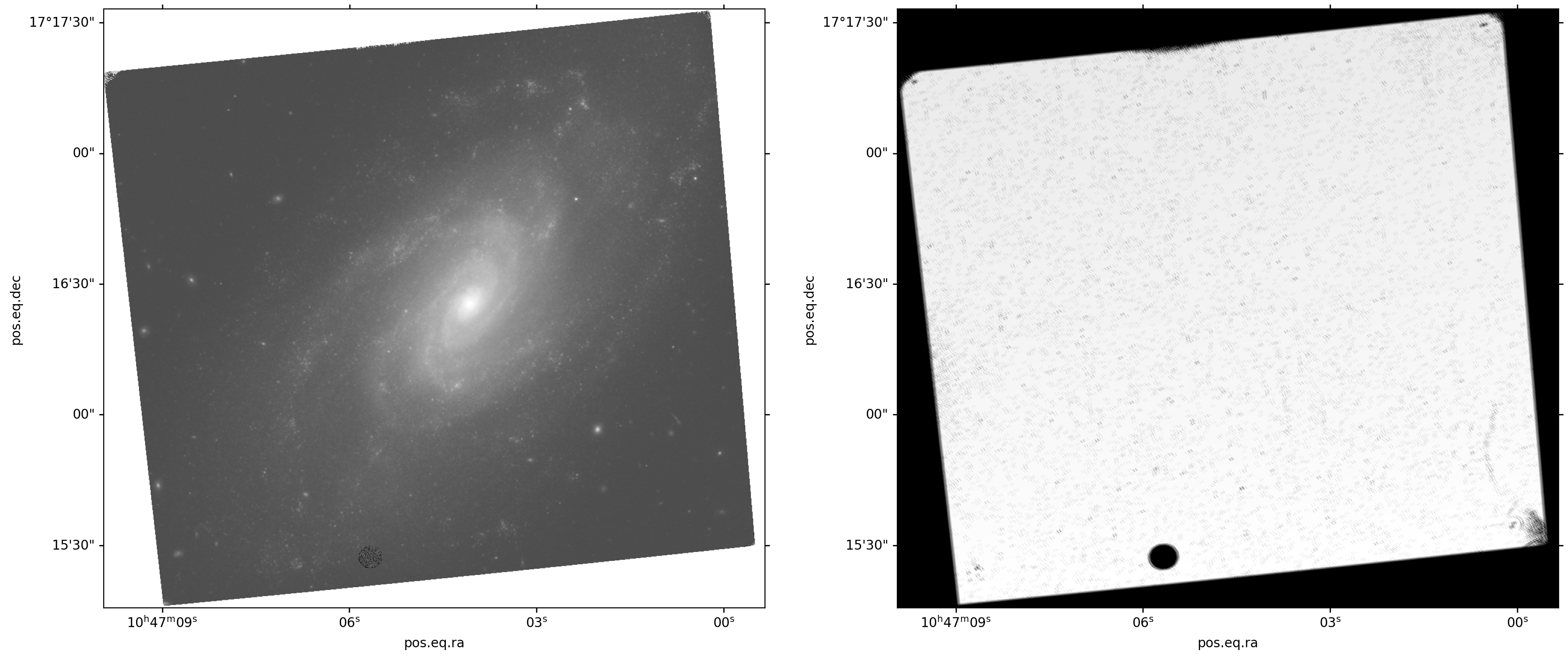
The drizzled science and weight images produced from the first call to AstroDrizzle with no optimization of the plate scale and pixfrac are plotted below.
with fits.open('f160w_noopt_drz.fits') as hdu:
    im1wcs = wcs.WCS(hdu[1].header)
    sci1 = hdu[1].data
    wht1 = hdu[2].data

norm1 = ImageNormalize(sci1, vmin=-0.05, vmax=100, stretch=LogStretch())
fig, ax = plt.subplots(1, 2, figsize=(20, 15), subplot_kw={'projection': im1wcs})
ax[0].imshow(sci1, norm=norm1, cmap='gray', origin='lower')
ax[1].imshow(wht1, cmap='gray', origin='lower')
The drizzled science image is on the left and the associated weight image is on the right, both without optimization of the plate scale and pixfrac.
To compare, the figure plotted below shows close ups of the same part of the sky from the two drizzled products.
radeclims = wcs.utils.pixel_to_skycoord([825, 875], [930, 980], im1wcs)

with fits.open('f160w_opt_drz.fits') as hdu:
    im2wcs = wcs.WCS(hdu[1].header)
    sci2 = hdu[1].data
    wht2 = hdu[2].data

norm1 = ImageNormalize(sci2, vmin=0.70, vmax=4.0, stretch=LogStretch())
norm2 = ImageNormalize(sci2, vmin=0.18, vmax=1.0, stretch=LogStretch())

fig = plt.figure(figsize=(16, 8))

ax = fig.add_subplot(1, 2, 1, projection=im1wcs)
ax.imshow(sci1, norm=norm1, cmap='gray')
ax.set_xlim(radeclims.to_pixel(im1wcs)[0])
ax.set_ylim(radeclims.to_pixel(im1wcs)[1])

ax = fig.add_subplot(1, 2, 2, projection=im2wcs)
ax.imshow(sci2, norm=norm2, cmap='gray')
ax.set_xlim(radeclims.to_pixel(im2wcs)[0])
ax.set_ylim(radeclims.to_pixel(im2wcs)[1])
The image on the left is without improved plate scale and pixfrac, and shows that the detector undersamples the PSF. The image on the right is the image with optimized parameters where the resolution is greatly improved.
5. Optimizing the final_pixfrac parameter#
While the optimized final_pixfrac in the example above was chosen from experience with using a four-point dither, the value that should be used is not known a priori. The value could be different depending on several factors. For example, if the number of images is greater than four, the value used for final_pixfrac could be smaller since more images are available to fill in holes in the output grid. On the other hand, it is possible that no dithering was used during the observations. In that case, final_pixfrac should be left at 1.0, since shrinking the size of the drop could be detrimental.
Below, a series of experiments will be run to determine the best final_pixfrac value for the selected output plate scale, by varying pixfrac in steps of 0.1 over a range of values from 0.1 to 1.0.
pixfracs = np.arange(0.1, 1.1, 0.1)

for pixfrac in pixfracs:
    outname = 'f160w_{:.1f}'.format(pixfrac)
    drizzlepac.astrodrizzle.AstroDrizzle(flt_files,
                                         output=outname,
                                         **selected_params,
                                         context=False,
                                         build=True,
                                         preserve=False,
                                         skymethod='match',
                                         driz_separate=False, median=False, blot=False, driz_cr=False, # CR-rej off
                                         final_pixfrac=pixfrac,
                                         final_wcs=True,
                                         final_rot=0.,
                                         final_scale=0.065)
clear_output()
When evaluating what value to use for final_pixfrac, THERE IS NO SINGLE METRIC THAT INDICATES WHAT VALUE TO USE, and several factors should be taken into account. The general philosophy is that the chosen value should improve the resolution of the image as much as possible, without causing any adverse effects.
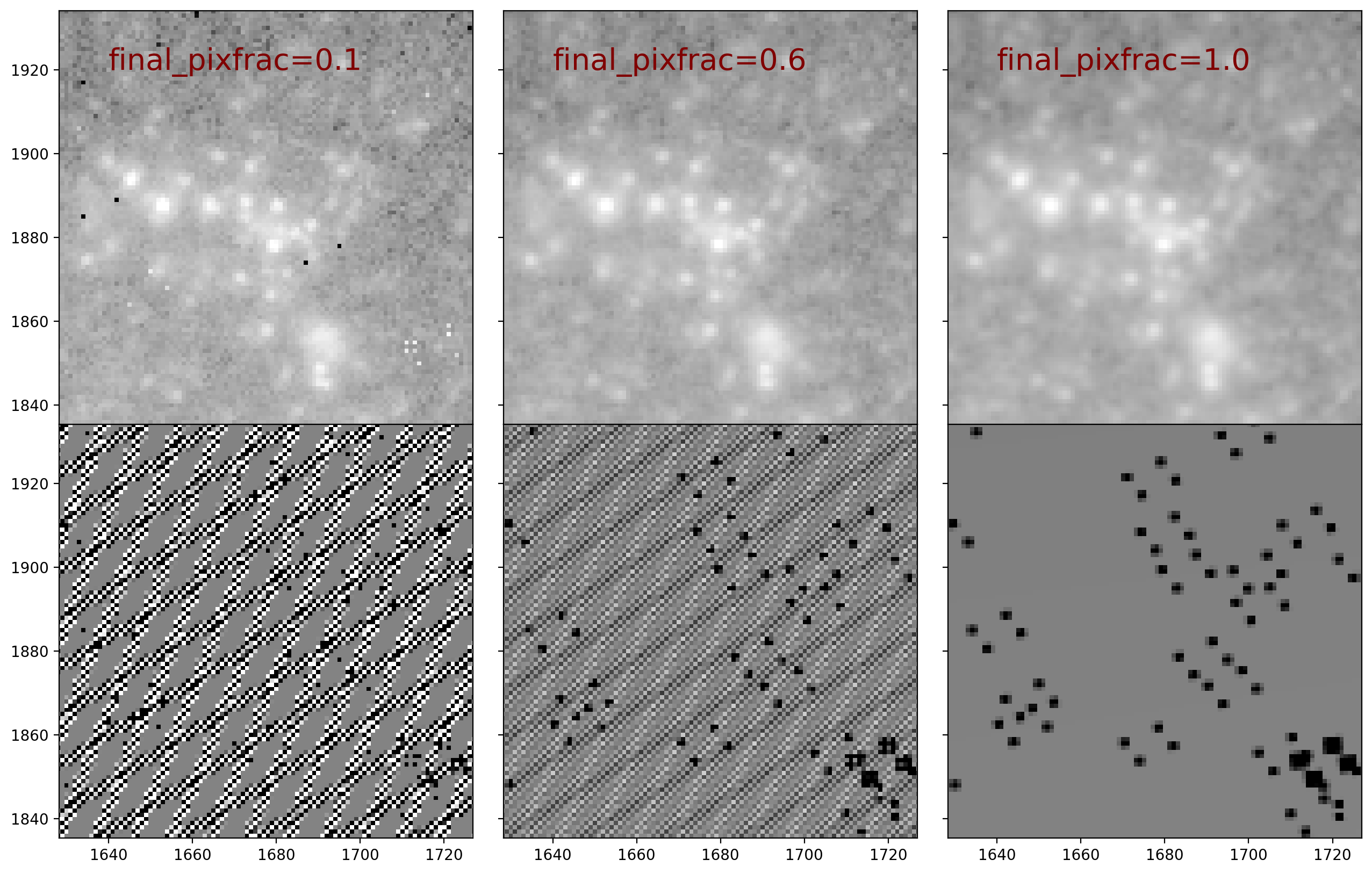
The first thing to look for is an excessive number of holes in the science and weight images. The figure below shows the central region of the science and weight images produced by three different final_pixfrac values.
with fits.open('f160w_0.1_drz.fits') as hdu1:
    sci1 = hdu1[1].data
    wht1 = hdu1[2].data

with fits.open('f160w_0.6_drz.fits') as hdu2:
    sci2 = hdu2[1].data
    wht2 = hdu2[2].data

with fits.open('f160w_1.0_drz.fits') as hdu3:
    sci3 = hdu3[1].data
    wht3 = hdu3[2].data

fig, ax = plt.subplots(2, 3, figsize=(16, 10), sharex=True, sharey=True)
fig.subplots_adjust(hspace=0, wspace=0)

norm3 = ImageNormalize(wht2, vmin=400, vmax=600, stretch=LinearStretch())
ax[0, 0].imshow(sci1, norm=norm2, cmap='gray')
ax[0, 0].text(1640, 1920, 'final_pixfrac=0.1', fontsize='20', color='maroon')
ax[0, 1].imshow(sci2, norm=norm2, cmap='gray')
ax[0, 1].text(1640, 1920, 'final_pixfrac=0.6', fontsize='20', color='maroon')
ax[0, 2].imshow(sci3, norm=norm2, cmap='gray')
ax[0, 2].text(1640, 1920, 'final_pixfrac=1.0', fontsize='20', color='maroon')
ax[1, 0].imshow(wht1, norm=norm3, cmap='gray')
ax[1, 1].imshow(wht2, norm=norm3, cmap='gray')
ax[1, 2].imshow(wht3, norm=norm3, cmap='gray')
ax[0, 0].set_xlim(radeclims.to_pixel(im2wcs)[0])
ax[0, 0].set_ylim(radeclims.to_pixel(im2wcs)[1])
This figure above shows the central region of the science and weight images produced by final_pixfrac values (left to right) of 0.1, 0.8 and 1.0. The top row is the science frame, the bottom is the weight image. The science image with the smallest final_pixfrac value of 0.1 shows a noisy background and holes in the image where no input pixels fall into the output grid because pixfrac is too small.
Inspection of the weight map corresponding to the smallest final_pixfrac value shows many places with weights of zero, indicating that a final_pixfrac value of 0.1 is clearly too small and was only included in this example for illustrative purposes.
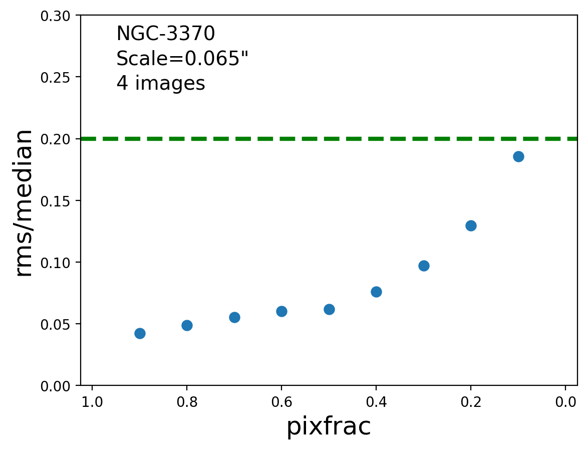
Another piece of information that can be useful is the amount of noise in the weight image. As suggested in the DrizzlePac Handbook Section 7.3, statistics performed on the drizzled weight image should yield a RMS/median value less than ~0.2. This threshold controls the trade-off between improving image resolution versus increasing background noise due to pixel resampling.
The final_pixfrac value should be small enough to avoid degrading the final drizzle-combined image, but large enough that when all images are “dropped” onto the final frame, coverage of the output frame is fairly uniform. In general, final_pixfrac should be slightly larger than the final output scale to allow some “spillover” to adjacent pixels. This will help avoid “holes” in the final product when a given pixel has been flagged as bad in several frames.
The figure below shows the RMS/median as a function of final_pixfrac. One should take care to use the same region in the weight image as the region where the object of interest is located in the science image. If one is using the entire image for scientific analysis, then one should measure the statistics of the weight image where there is more variance.
whtlist = glob.glob('f160w_0.[0-9]*drz.fits')

std_med = np.empty(len(whtlist), dtype=float)
fraclist = np.empty(len(whtlist), dtype=float)
xlims = radeclims.to_pixel(im1wcs)[0].astype(int)
ylims = radeclims.to_pixel(im1wcs)[1].astype(int)

# Loop that measures statistics, also some information gathering
for i, im in enumerate(whtlist):
    with fits.open(im) as hdu:
        hdr = hdu[0].header
        wht = hdu[2].data
    if i == 0:
        target = hdr['TARGNAME']
        scale = str(hdr['D001SCAL'])
        nimg = hdr['NDRIZIM']
    wht_std = np.std(wht[ylims[0]: ylims[1], xlims[0]: xlims[1]])
    wht_med = np.median(wht[ylims[0]: ylims[1], xlims[0]: xlims[1]])
    std_med[i] = wht_std / wht_med
    fraclist[i] = hdr['D001PIXF']

# Plotting commands
plt.clf()
plt.xlim(1.025, -0.025)
plt.ylim(0., 0.3)
plt.scatter(fraclist, std_med, s=50)
plt.axhline(0.2, ls='--', lw=3, c='g')
plt.xlabel('pixfrac', fontsize=18)
plt.ylabel('rms/median', fontsize=18)
plt.text(0.95, 0.28, target, fontsize=14, horizontalalignment='left')
plt.text(0.95, 0.26, 'Scale=' + str(scale) + '"', fontsize=14, horizontalalignment='left')
plt.text(0.95, 0.24, str(nimg) + ' images', fontsize=14, horizontalalignment='left')
Note that none of the test images have RMS/median greater than 0.2, so this does not seem to be a good metric for WFC3/IR in which the PSF is undersampled. (We suspect that this recommendation from the DrizzlePac Handbook was based on WFC3/UVIS or ACS/WFC dithered frames.)
The RMS/median increases steadily to a final_pixfrac value of 0.5, where there is a change in the slope of the function. For an output scale of 0.065”/pix (0.5 times the native plate scale) thus select the pixfrac 0.6 for the final drizzled image.
6. Final thoughts#
The final_pixfrac value has to be small enough to avoid degrading the combined output image, but large enough that when all images are “dropped” onto the final frame, coverage of the output frame is fairly uniform. In general, final_pixfrac should be slightly larger than the final output scale to allow some “spillover” to adjacent pixels. This will help avoid “holes” in the final product when a given pixel has been flagged as “bad” in several frames. Optimizing the final drizzle parameters is a balance between the benefits of improving the image resolution and PSFs at the expense of increasing noise in the background.
About this Notebook#
Created: 12 Dec 2018;     R. Avila
Updated: 30 Dec 2024;     R. Avila & J. Mack
Source: GitHub spacetelescope/hst_notebooks
Additional Resources#
Below are some additional resources that may be helpful. Please send any questions through the HST Help Desk.
Citations#
If you use Python packages such as astropy, astroquery, drizzlepac, matplotlib, or numpy for published research, please cite the authors.
Follow these links for more information about citing various packages:
