1D Spectra Extraction

Learning Goals

• 0 Introduction
  • 0.1 Import Necessary Packages
  • 0.2 Collect Data Set From the MAST Archive Using Astroquery
• 1 x1d FITS File Structure
• 2 Plot the Extraction Region
• 3 Extracted Spectra of STIS Echelle

0 Introduction

The x1d FITS file is the one-dimensional extracted spectra for individual imsets of flt, sfl, or crj images. The x1d file is in binary table with the science information stored in the ‘SCI’ extension. In this notebook, we will show how to visualize the extraction regions when generating the x1d extracted spectra from a flt image. In some cases when users work with images with multiple sources or extended background, they might want to customize extraction. The goal of visualizing extraction region is to help confirm that the proper extraction parameters are selected, and the extraction regions do not overlap.

For more information on extracted spectra, see the STIS Data Handbook: 5.5 Working with Extracted Spectra

0.1 Import Necessary Packages

• astropy.io.fits and astropy.table.Table for accessing FITS files

• astroquery.mast.Observations for finding and downloading data from the MAST archive

• os for managing system paths

• numpy to handle array functions

• stistools for operations on STIS Data

• matplotlib for plotting data

# Import for: Reading in fits file
from astropy.io import fits
from astropy.table import Table

# Import for: Downloading necessary files. (Not necessary if you choose to collect data from MAST)
from astroquery.mast import Observations

# Import for: Managing system variables and paths
import os

# Import for: Quick Calculation and Data Analysis
import numpy as np

# Import for: Operations on STIS Data
# import stistools

# Import for: Plotting and specifying plotting parameters
import matplotlib
%matplotlib inline
from matplotlib import pyplot as plt
# from matplotlib.ticker import FixedLocator

matplotlib.rcParams['image.origin'] = 'lower'
matplotlib.rcParams['image.cmap'] = 'viridis'
matplotlib.rcParams['image.interpolation'] = 'none'

0.2 Collect Data Set From the MAST Archive Using Astroquery

There are other ways to download data from MAST such as using CyberDuck. The steps of collecting data is beyond the scope of this notebook, and we are only showing how to use astroquery.

# change this field in you have a specific dataset to be explored
obs_id = 'odj102010'
# Search target object by obs_id
target = Observations.query_criteria(obs_id=obs_id)
# get a list of files assiciated with that target
target_list = Observations.get_product_list(target)
# Download fits files
result = Observations.download_products(target_list, extension=['_flt.fits', '_x1d.fits'], productType=['SCIENCE'])
flt_filename = os.path.join(f'./mastDownload/HST/{obs_id}/{obs_id}_flt.fits')
x1d_filename = os.path.join(f'./mastDownload/HST/{obs_id}/{obs_id}_x1d.fits')

Downloading URL https://mast.stsci.edu/api/v0.1/Download/file?uri=mast:HST/product/odj102010_flt.fits to ./mastDownload/HST/odj102010/odj102010_flt.fits ...

 [Done]

Downloading URL https://mast.stsci.edu/api/v0.1/Download/file?uri=mast:HST/product/odj102010_x1d.fits to ./mastDownload/HST/odj102010/odj102010_x1d.fits ...

 [Done]

1 x1d FITS File Structure

The x1d file is a multi-extension FITS file with header information stored in the primary extension (note that for CCD data the similar extension is sx1), and the science data stored in the first extension called “SCI”.

fits.info(x1d_filename)

Filename: ./mastDownload/HST/odj102010/odj102010_x1d.fits
No.    Name      Ver    Type      Cards   Dimensions   Format
  0  PRIMARY       1 PrimaryHDU     274   ()      
  1  SCI           1 BinTableHDU    157   1R x 19C   [1I, 1I, 1024D, 1024E, 1024E, 1024E, 1024E, 1024E, 1024E, 1024I, 1E, 1E, 1I, 1E, 1E, 1E, 1E, 1024E, 1E]   

The SCI extension contains the science data of the spectra along the spectral direction such as the wavelength and the flux, and information on the extraction region and the background region when performing the 1D spectra extraction:

Column name	Description	Data Type
EXTRLOCY	an array that gives the location of the center of the spectral trace for each pixel along the Y direction	float32 array[1024]
A2CENTER	row number in the y direction at which the spectral trace is centered	float32
EXTRSIZE	height of extraction region	float32
BK1SIZE	height of background region above the extraction region	float32
BK2SIZE	height of background region below the extraction region	float32
BK1OFFST	background region offset from the center of the extraction region above the extraction region	float32
BK2OFFST	background region offset from the center of the extraction region below the extraction region	float32

cols = ['SPORDER', 'WAVELENGTH', 'FLUX', 'EXTRLOCY', 'A2CENTER', 'EXTRSIZE', 'BK1SIZE', 'BK2SIZE', 'BK1OFFST', 'BK2OFFST']
Table.read(x1d_filename)[cols]

WARNING: UnitsWarning: 'Angstroms' did not parse as fits unit: At col 0, Unit 'Angstroms' not supported by the FITS standard. Did you mean Angstrom or angstrom? If this is meant to be a custom unit, define it with 'u.def_unit'. To have it recognized inside a file reader or other code, enable it with 'u.add_enabled_units'. For details, see https://docs.astropy.org/en/latest/units/combining_and_defining.html [astropy.units.core]
WARNING: UnitsWarning: 'Counts/s' did not parse as fits unit: At col 0, Unit 'Counts' not supported by the FITS standard. Did you mean count? If this is meant to be a custom unit, define it with 'u.def_unit'. To have it recognized inside a file reader or other code, enable it with 'u.add_enabled_units'. For details, see https://docs.astropy.org/en/latest/units/combining_and_defining.html [astropy.units.core]
WARNING: UnitsWarning: 'erg/s/cm**2/Angstrom' contains multiple slashes, which is discouraged by the FITS standard [astropy.units.format.generic]

Table length=1

SPORDER	WAVELENGTH	FLUX	EXTRLOCY	A2CENTER	EXTRSIZE	BK1SIZE	BK2SIZE	BK1OFFST	BK2OFFST
	Angstroms	erg / (Angstrom s cm2)	pix	pix	pix	pix	pix	pix	pix
int16	float64[1024]	float32[1024]	float32[1024]	float32	float32	float32	float32	float32	float32
1	1513.611692349868 .. 1567.668670092399	1.96904e-12 .. 9.89624e-14	382.2857 .. 397.2364	389.5777	11	5	5	-300	300

Note that X1D columns in pixel units (e.g. EXTRLOCY) are in one-indexed coordinates. Thus when visualizing the extraction region with Python (zero-indexed), the pixel coordinates need to be subtracted by 1. Additionally, the n-th pixel (in one-index coordinates) ranges from n-0.5 to n+0.5.

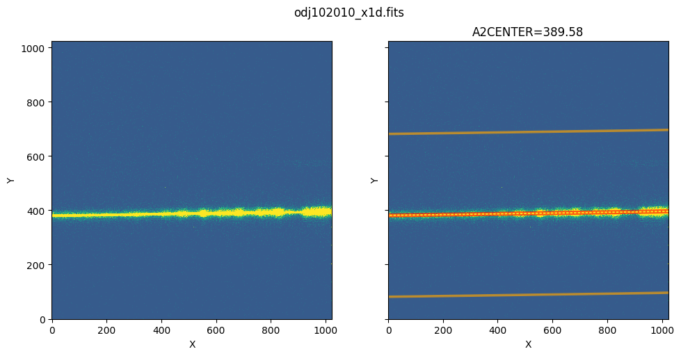
2 Plot the Extraction Region

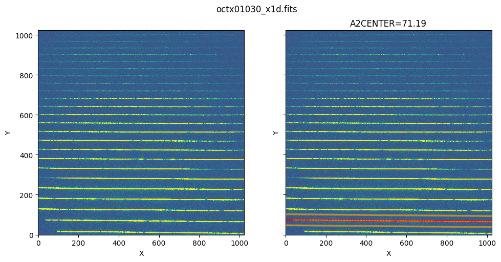
Left: The 2D FLT image.

Right: The 2D FLT image with extraction regions over-plotted. The extraction region is plotted in red, and the 2 background regions are plotted in orange.

To zoom in to a specific region along the Y axis, pass in the optional parameter yrange.

def show_extraction_regions(x1d_filename, flt_filename, sci_ext=1, row=0, xrange=None, yrange=None):
    
    fig, axes = plt.subplots(1, 2, sharey=True)
    fig.tight_layout()
    fig.subplots_adjust(wspace=0.2, hspace=0.2, top=0.88)
    fig.set_figwidth(10)
    fig.set_figheight(5)
    fig.suptitle(os.path.basename(x1d_filename))
    
    x1d = fits.getdata(x1d_filename, ext=sci_ext)[row]
    flt = fits.getdata(flt_filename, ext=('SCI', sci_ext))
    
    # LEFT & Right PLOTS:
    for ax in axes[0:2]:
        # Display the 2D FLT spectrum on the left:
        ax.imshow(flt, origin='lower', interpolation='none', aspect='auto', vmin=-6, vmax=15)
        ax.set_xlabel('X')
        ax.set_ylabel('Y')

    # Right PLOT:
    axes[1].set_title(f"A2CENTER={x1d['A2CENTER']:.2f}")
    # Extraction region in red:
    axes[1].plot(np.arange(1024), 
                 x1d['EXTRLOCY'] - 1, 'r:', alpha=0.6)
    axes[1].plot(np.arange(1024), 
                 x1d['EXTRLOCY'] - 1 - x1d['EXTRSIZE']//2,
                 color='red', alpha=0.6)
    axes[1].plot(np.arange(1024), 
                 x1d['EXTRLOCY'] - 1 + x1d['EXTRSIZE']//2,
                 color='red', alpha=0.6)
    # Background regions in orange:
    axes[1].plot(np.arange(1024), 
                 x1d['EXTRLOCY'] - 1 + x1d['BK1OFFST'] - x1d['BK1SIZE']//2,
                 color='orange', alpha=0.6)
    axes[1].plot(np.arange(1024), 
                 x1d['EXTRLOCY'] - 1 + x1d['BK1OFFST'] + x1d['BK1SIZE']//2,
                 color='orange', alpha=0.6)
    axes[1].plot(np.arange(1024), 
                 x1d['EXTRLOCY'] - 1 + x1d['BK2OFFST'] - x1d['BK2SIZE']//2, 
                 color='orange', alpha=0.6)
    axes[1].plot(np.arange(1024), 
                 x1d['EXTRLOCY'] - 1 + x1d['BK2OFFST'] + x1d['BK2SIZE']//2, 
                 color='orange', alpha=0.6)
    
    axes[0].set_xlim(-0.5, 1023.5)
    axes[0].set_ylim(-0.5, 1023.5)
    axes[1].set_xlim(-0.5, 1023.5)
    axes[1].set_ylim(-0.5, 1023.5)
    
    if xrange is not None:
        axes[0].set_xlim(xrange[0], xrange[1])
        axes[1].set_xlim(xrange[0], xrange[1])
    if yrange is not None:
        axes[0].set_ylim(yrange[0], yrange[1])
        axes[1].set_ylim(yrange[0], yrange[1])

show_extraction_regions(x1d_filename, flt_filename)

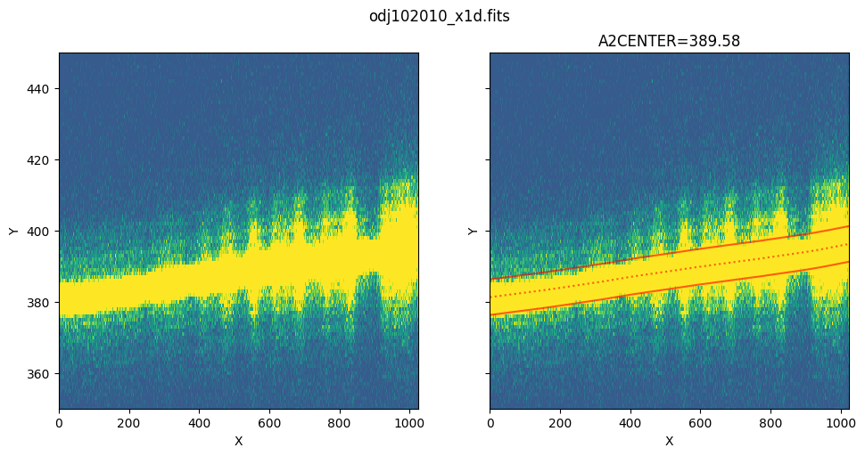
Zoom in to the extraction region:

show_extraction_regions(x1d_filename, flt_filename, yrange=[350, 450])

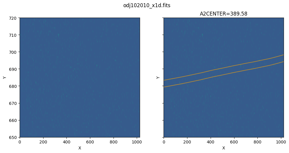
Zoom in to the background region above the extraction region:

show_extraction_regions(x1d_filename, flt_filename, yrange=[650, 720])

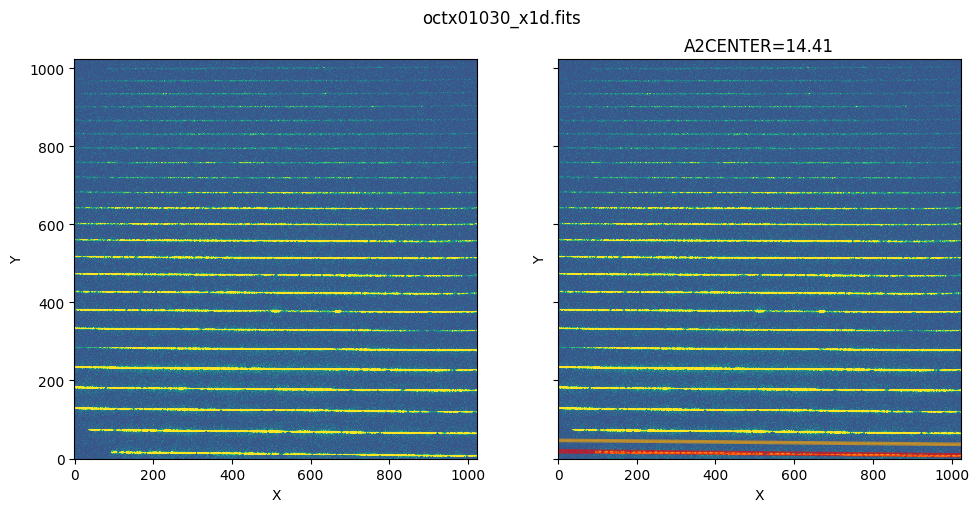
3 Extracted Spectra of STIS Echelle

The method of visualizing the extracted region also applies to echelle data, except that echelle data has multiple spectra orders, and therefore has multiple EXTRLOCY corresponding to each SPORDER. In the plotting method, there is a parameter called ‘row’ which specifies the SPORDER we want to extract. We’ll show how to visualize the extracted region for STIS echelle data.

# Download the octx01030 dataset, which is a NUV-MAMA echelle data
obs_id = 'octx01030'
# Search target objscy by obs_id
target = Observations.query_criteria(obs_id=obs_id)
# get a list of files assiciated with that target
echelle_list = Observations.get_product_list(target)
# Download fits files
result = Observations.download_products(echelle_list, extension=['_flt.fits', '_x1d.fits'], productType=['SCIENCE',])
echelle_flt = os.path.join(f'./mastDownload/HST/{obs_id}/{obs_id}_flt.fits')
echelle_x1d = os.path.join(f'./mastDownload/HST/{obs_id}/{obs_id}_x1d.fits')

Downloading URL https://mast.stsci.edu/api/v0.1/Download/file?uri=mast:HST/product/octx01030_flt.fits to ./mastDownload/HST/octx01030/octx01030_flt.fits ...

 [Done]

Downloading URL https://mast.stsci.edu/api/v0.1/Download/file?uri=mast:HST/product/octx01030_x1d.fits to ./mastDownload/HST/octx01030/octx01030_x1d.fits ...

 [Done]

As shown in the table data, there are multiple rows with each row having a different SPORDER. Each row also has different EXTRLOCY, which corresponds to different extraction regions in the flt image for each SPORDER.

cols = ['SPORDER', 'WAVELENGTH', 'FLUX', 'EXTRLOCY', 'EXTRSIZE', 'BK1SIZE', 'BK2SIZE', 'BK1OFFST', 'BK2OFFST']
Table.read(echelle_x1d, hdu=1)[cols]

WARNING: UnitsWarning: 'Angstroms' did not parse as fits unit: At col 0, Unit 'Angstroms' not supported by the FITS standard. Did you mean Angstrom or angstrom? If this is meant to be a custom unit, define it with 'u.def_unit'. To have it recognized inside a file reader or other code, enable it with 'u.add_enabled_units'. For details, see https://docs.astropy.org/en/latest/units/combining_and_defining.html [astropy.units.core]
WARNING: UnitsWarning: 'Counts/s' did not parse as fits unit: At col 0, Unit 'Counts' not supported by the FITS standard. Did you mean count? If this is meant to be a custom unit, define it with 'u.def_unit'. To have it recognized inside a file reader or other code, enable it with 'u.add_enabled_units'. For details, see https://docs.astropy.org/en/latest/units/combining_and_defining.html [astropy.units.core]
WARNING: UnitsWarning: 'erg/s/cm**2/Angstrom' contains multiple slashes, which is discouraged by the FITS standard [astropy.units.format.generic]

Table length=24

SPORDER	WAVELENGTH	FLUX	EXTRLOCY	EXTRSIZE	BK1SIZE	BK2SIZE	BK1OFFST	BK2OFFST
	Angstroms	erg / (Angstrom s cm2)	pix	pix	pix	pix	pix	pix
int16	float64[1024]	float32[1024]	float32[1024]	float32	float32	float32	float32	float32
66	3067.682086855123 .. 3119.012536891768	-2.030472e-14 .. 2.9376e-12	19.45284 .. 9.476334	7	5	5	28.01995	-28.77343
67	3021.857427057288 .. 3072.451049005796	-1.021074e-14 .. 3.076689e-12	75.95515 .. 66.73722	7	5	5	27.28738	-28.01995
68	2977.380919809147 .. 3027.257338502545	-3.754732e-14 .. 1.087724e-12	131.2862 .. 122.4106	7	5	5	26.57536	-27.28738
69	2934.193937243135 .. 2983.372006818285	-2.190875e-14 .. 2.144429e-12	184.4561 .. 176.3899	7	5	5	25.88353	-26.57536
70	2892.241202288543 .. 2940.739046013224	-1.478441e-14 .. 3.037708e-12	236.3518 .. 228.9839	7	5	5	25.21152	-25.88353
71	2851.470552660116 .. 2899.305600220004	-3.966172e-15 .. 2.761381e-12	286.8198 .. 280.1042	7	5	5	24.55895	-25.21152
72	2811.832724517215 .. 2859.021746954763	-7.334717e-15 .. 7.610627e-13	335.8839 .. 329.9276	7	5	5	23.92547	-24.55895
73	2773.281153907109 .. 2819.840296387559	-1.893139e-14 .. 1.559154e-12	383.655 .. 378.4149	7	5	5	23.31071	-23.92547
74	2735.771794309852 .. 2781.716606874576	-6.107451e-15 .. 6.842402e-13	430.1284 .. 425.6361	7	5	5	22.7143	-23.31071
...	...	...	...	...	...	...	...	...
80	2530.413003679701 .. 2572.968492248937	-2.266979e-15 .. 6.605272e-13	684.3518 .. 683.5427	7	5	5	19.50066	-19.99467
81	2499.145134209817 .. 2541.180702698945	-2.67421e-15 .. 4.349387e-13	723.0336 .. 722.7673	7	5	5	19.02243	-19.50066
82	2468.640092359287 .. 2510.167438601849	-2.455758e-15 .. -1.745655e-14	760.7408 .. 761.0947	7	5	5	18.55963	-19.02243
83	2438.870300747431 .. 2479.900734272652	-2.494167e-15 .. 4.517789e-14	797.6779 .. 798.4939	7	5	5	18.11187	-18.55963
84	2409.809495426899 .. 2450.35395445196	-2.180459e-14 .. -1.227559e-13	833.6877 .. 835.0537	7	5	5	17.6788	-18.11187
85	2381.432648611571 .. 2421.501716113727	-2.473746e-15 .. 6.20382e-14	868.6304 .. 870.5798	7	5	5	17.26004	-17.6788
86	2353.715896795153 .. 2393.319815723954	-3.907116e-15 .. 7.426204e-16	903.1175 .. 905.5428	7	5	5	16.85524	-17.26004
87	2326.636473828409 .. 2365.785161512079	-2.284579e-15 .. -2.450691e-13	936.36 .. 939.4832	7	5	5	16.46401	-16.85524
88	2300.172648559522 .. 2338.875710356606	-2.107181e-15 .. -1.893928e-13	969.1404 .. 972.7743	7	5	5	16.08601	-16.46401
89	2274.303666679877 .. 2312.570408922325	-1.849008e-15 .. -2.878802e-13	1001.03 .. 1005.438	7	5	5	15.72085	-16.08601

show_extraction_regions(echelle_x1d, echelle_flt)

Similarly, we can show the extraction region of the next SPORDER by passing the row number into the plotting method:

show_extraction_regions(echelle_x1d, echelle_flt, row=1)

After visualizing the extraction, we can use the x1d() function in stistools to customize extraction. For more information, see x1d.

---

About this Notebook

Author: Keyi Ding

Updated On: 2023-01-05

This tutorial was generated to be in compliance with the STScI style guides and would like to cite the Jupyter guide in particular.

Citations

If you use astropy, matplotlib, astroquery, or numpy for published research, please cite the authors. Follow these links for more information about citations:

• Citing astropy/numpy/matplotlib

• Citing astroquery

---

Top of Page