
WFC3 Image Displayer & Analyzer#
Learning Goals#
This notebook provides a method to quickly display images from the Hubble Space Telescope’s Wide Field
Camera 3 (WFC3) instrument. This tool also allows the user to derive statistics by row or column in the image.
By the end of this tutorial, you will:
Download two WFC3 images from MAST.
Learn how to use the
display_imagetool to display any WFC3 fits file.Learn how to use the
row_column_statstool to plot row or column statistics for any WFC3 fits file.
Table of Contents#
Introduction
1. Imports
2. Query MAST and download a WFC3 flt.fits and ima.fits image
3. display_image
3.1 Display the full images with metadata
3.2 Display UVIS1 & UVIS2 separately
3.3 Display an image section and change the SCI array colormap
3.4 Change the scaling of the SCI and ERR arrays
3.5 Display each read of ima image section
4. row_column_stats
4.1 Compute column median and column standard deviation for a full image
4.2 Measure UVIS1 & UVIS2 column medians separately and overplot on one figure
4.3 Display image section and compute column & row mean
4.4 Compute column mean for each read of ima image section
5. Conclusions
Additional Resources
About the Notebook
Citations
Introduction#
One of the crucial steps in any analysis of WFC3 data is to visually inspect the
images. Whether you are viewing every image in the dataset or just a few
suspected outliers, displaying fits images takes time. To speed up the process
of displaying WFC3 images, we have created a tool in Python, display_image(),
that is meant to be used in a Jupyter Notebook. Once the function is imported
into your Jupyter Notebook session, you enter the WFC3 fits image you
want to display and it shows the full science, error, and data quality arrays
with a good scaling and colorbar. If the observation is a full frame UVIS
exposure, then the two CCDs are displayed together as one image (i.e. a 4kx4k
image). The display_image() tool allows for some customization, such as
displaying only a section of the image as well as changing the colormap or scaling.
In addition to visually inspecting WFC3 exposures, it can be helpful to compute
and plot statistics of the image as well. One common technique to quantify WFC3
images during analysis is to measure statistics of each individual column or row.
In this notebook we present a tool in Python, row_column_stats(), that is
meant to be used in a Jupyter Notebook. After importing the function into your
notebook session, you enter a WFC3 fits image along with the axis and
statistic you are interested in measuring. The function returns a plot of the
row (or column) statistic as a function of row (or column) number. In addition
to the plot, the function returns the row/column values and statistics being plotted.
This is useful if you want to plot multiple images on one figure. The
row_column_stats() tool allows for some customization, such as measuring
only a section of the image as well as choosing the axis (row or column) and the
statistic (mean, median, mode, or, standard deviation).
1. Imports#
We import:
Package Name |
Purpose |
|---|---|
|
setting environment variables |
|
downloading data from MAST |
|
plotting data |
|
displaying any WFC3 image |
|
computing statistics on a WFC3 image |
import os

from astroquery.mast import Observations
import matplotlib.pyplot as plt

from display_image import display_image
from row_column_stats import row_column_stats

%matplotlib inline
2. Query MAST and download a WFC3 flt.fits and ima.fits image#
You may download the data from MAST using either the Archive Search Engine or the MAST Portal.
Here, we download our images via astroquery. For more information, please look at the documentation for
Astroquery, Astroquery.mast, and
CAOM Field Descriptions, which is used for the obs_table variable.
We download images of N2525 from proposal 15145, one being a flt.fits in WFC3/UVIS and the other
being a ima.fits in WFC3/IR. After downloading the images, we move them to our current working directory (cwd).
query = [('idgga5*', 'UVIS', 'FLT', (2, 3)),
         ('i*', 'IR', 'IMA', (10, 11))]

for criteria in query:
    # Get the observation records
    obs_table = Observations.query_criteria(obs_id=criteria[0], proposal_id=15145, target_name='N2525', instrument_name=f"WFC3/{criteria[1]}")

    # Get the listing of data products
    products = Observations.get_product_list(obs_table)

    # Filter the products for the file type
    filtered_products = Observations.filter_products(products, productSubGroupDescription=criteria[2], dataproduct_type='image')

    # Display the table
    filtered_products[criteria[3][0]:criteria[3][1]]

    # Download the images above
    download_table = Observations.download_products(filtered_products[criteria[3][0]:criteria[3][1]], mrp_only=False)

    # For convenience move file to cwd and remove empty download dir
    for file in download_table['Local Path']:
        filename = file.split('/')[-1]
        os.rename(file, os.path.basename(file))
        os.rmdir('mastDownload/HST/'+filename[:9])

    os.rmdir('mastDownload/HST/')
    os.rmdir('mastDownload/')
Downloading URL https://mast.stsci.edu/api/v0.1/Download/file?uri=mast:HST/product/idgga5m1q_flt.fits to ./mastDownload/HST/idgga5m1q/idgga5m1q_flt.fits ...
[Done]
Downloading URL https://mast.stsci.edu/api/v0.1/Download/file?uri=mast:HST/product/idggabk1q_ima.fits to ./mastDownload/HST/idggabk1q/idggabk1q_ima.fits ...
[Done]
List the fits files to verify they were moved properly
!ls -ltr *.fits
-rw-r--r-- 1 runner runner 168796800 Dec  2 20:15 idgga5m1q_flt.fits
-rw-r--r-- 1 runner runner 126201600 Dec  2 20:16 idggabk1q_ima.fits
3. display_image#
In this section, we demonstrate the functionality of display_image, a useful tool for quickly analyzing WFC3 images.
The subsections explain how to display full images with metadata, individual WFC3/UVIS chip images, a section of an
image with various colormaps/scaling, and individual WFC3/IR ima reads.
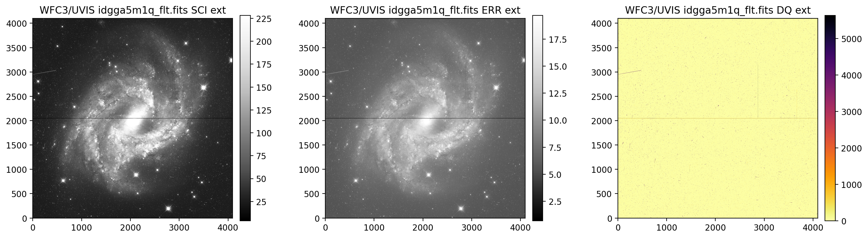
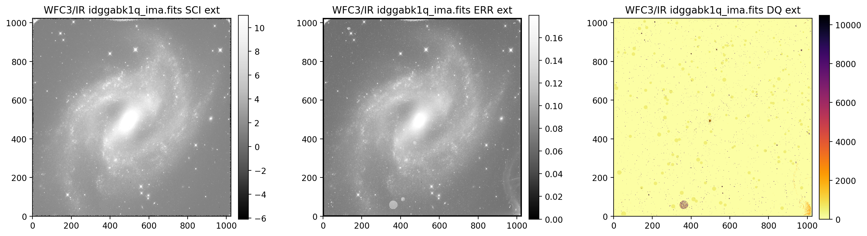
3.1 Display the full images with metadata#
First, we display the SCI, ERR, and DQ arrays for each image and print header info. The default value for printmeta
is False. In the cell below, we set the keyword printmeta to True to print useful information from the header of the
file to the screen. The WFC3/UVIS image is in electrons and the WFC3/IR image is in electrons/second. See Section 2.2.3
of the WFC3 Data Handbook for full descriptions of SCI, ERR, and DQ arrays.
display_image('idgga5m1q_flt.fits', printmeta=True)
display_image('idggabk1q_ima.fits', printmeta=True)
	WFC3/UVIS idgga5m1q_flt.fits
--------------------------------------------
Filter = F350LP, Date-Obs = 2018-03-04 T21:11:43,
Target = N2525, Exptime = 355.0, Subarray = False, Units = ELECTRONS
	WFC3/IR idggabk1q_ima.fits
--------------------------------------------
Filter = F160W, Date-Obs = 2018-09-11 T18:16:13,
Target = N2525, Exptime = 502.936462, Subarray = False, Units = ELECTRONS/S
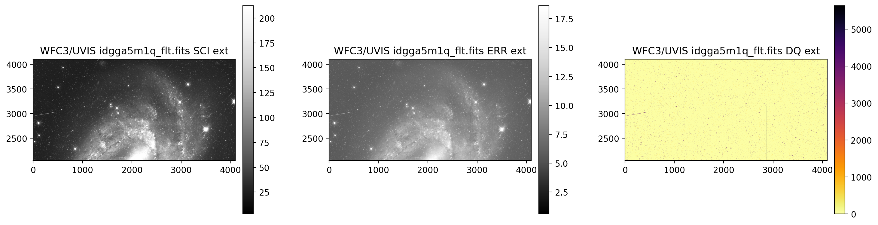
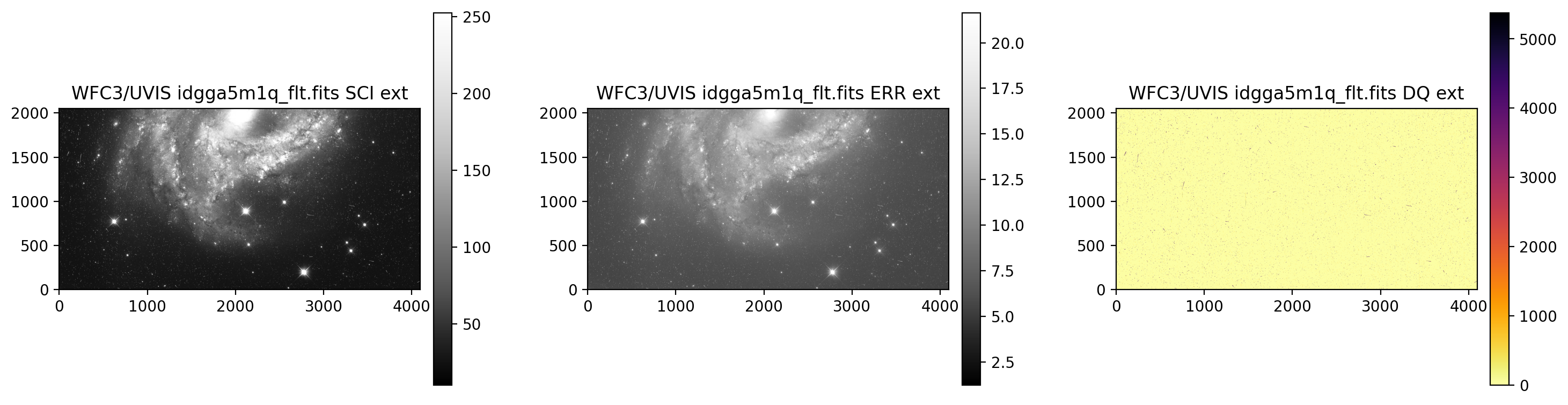
3.2 Display UVIS1 & UVIS2 separately#
Next, we display the WFC3/UVIS chips separately. To select a section of an image, append [xstart:xend,ystart:yend] to the
image name as shown below. Notice how we need to specify the full axis range [0:4096,0:2051] and not simply just
[:,:2051] as in standard numpy notation.
print('Display UVIS1')
display_image('idgga5m1q_flt.fits[0:4096,2051:4102]')
Display UVIS1
print('Display UVIS2')
display_image('idgga5m1q_flt.fits[0:4096,0:2051]')
Display UVIS2
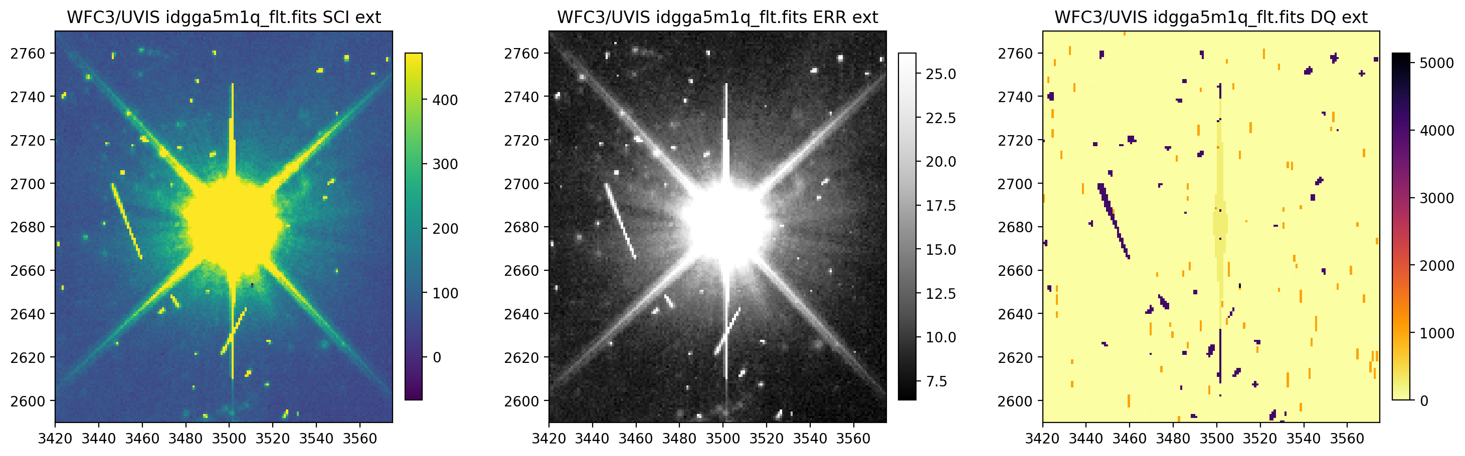
3.3 Display an image section and change the SCI array colormap#
Then, we display SCI arrays with a different colormap. Regardless of how many colormaps are being changed, all three
colormaps must be provided. The elements of colormaps sequentially correspond with the SCI, ERR, and DQ arrays.
display_image('idgga5m1q_flt.fits[3420:3575,2590:2770]',
              colormaps=["viridis", "Greys_r", "inferno_r"])
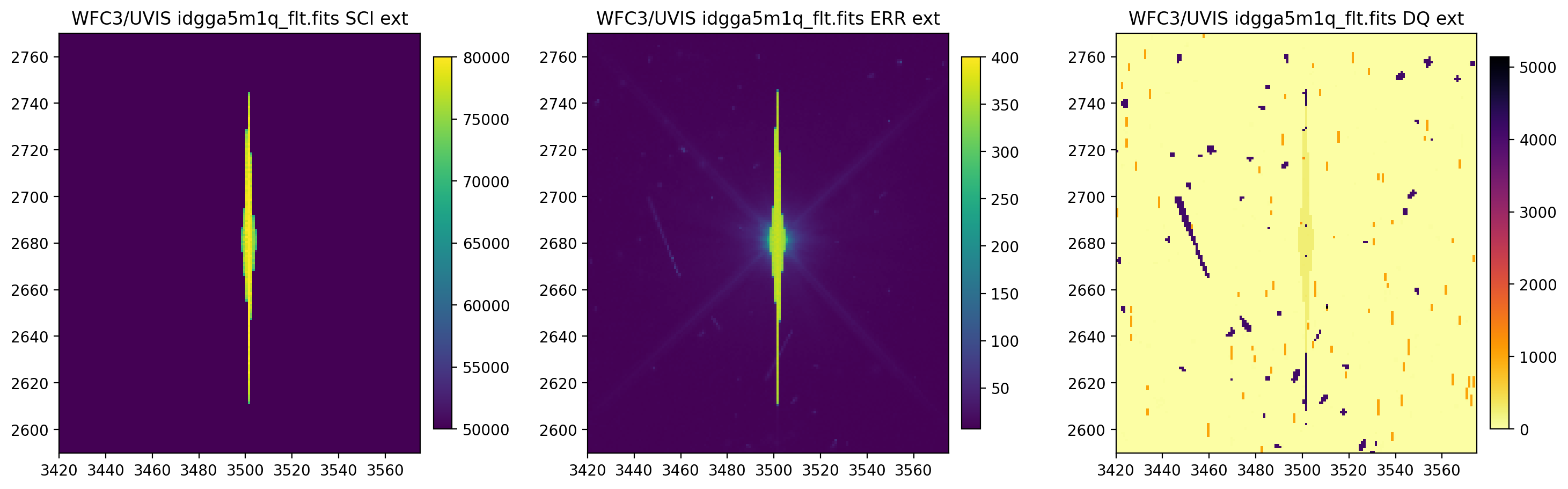
3.4 Change the scaling of the SCI and ERR arrays#
Now, we change the scaling of the SCI and ERR arrays. Regardless of how many scalings are being changed, all three
scalings must be provided. The elements of scaling sequentially correspond with the SCI, ERR, and DQ arrays.
The default scaling value of None uses astropy.visualization.ZScaleInterval() for scaling
(see documentation for more information).
display_image('idgga5m1q_flt.fits[3420:3575,2590:2770]',
              colormaps=["viridis", "viridis", "inferno_r"],
              scaling=[(50000, 80000), (None, 400), (None, None)])
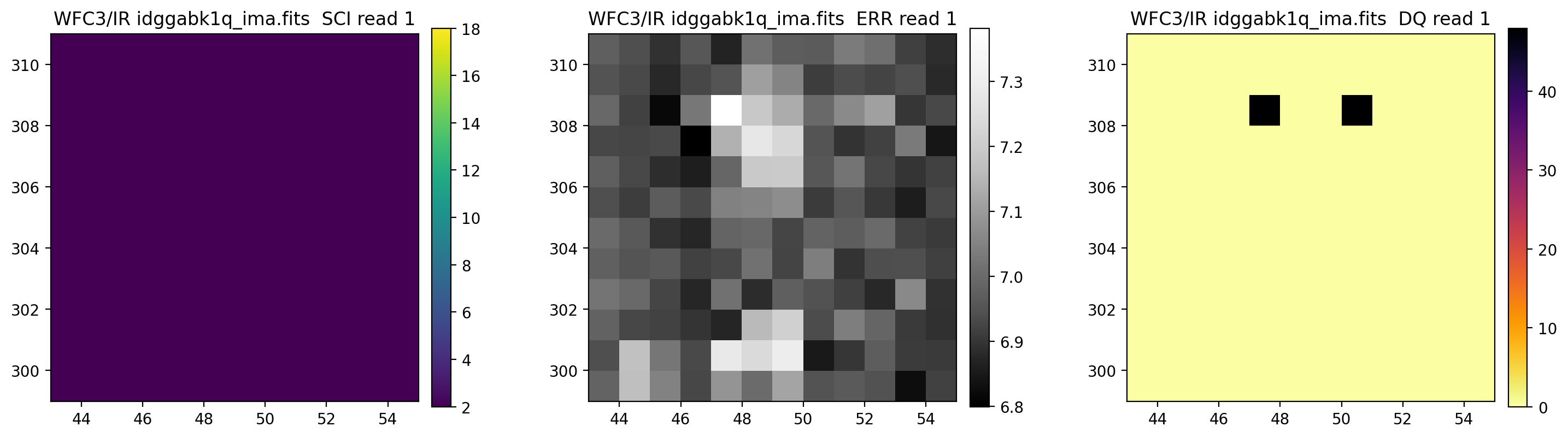
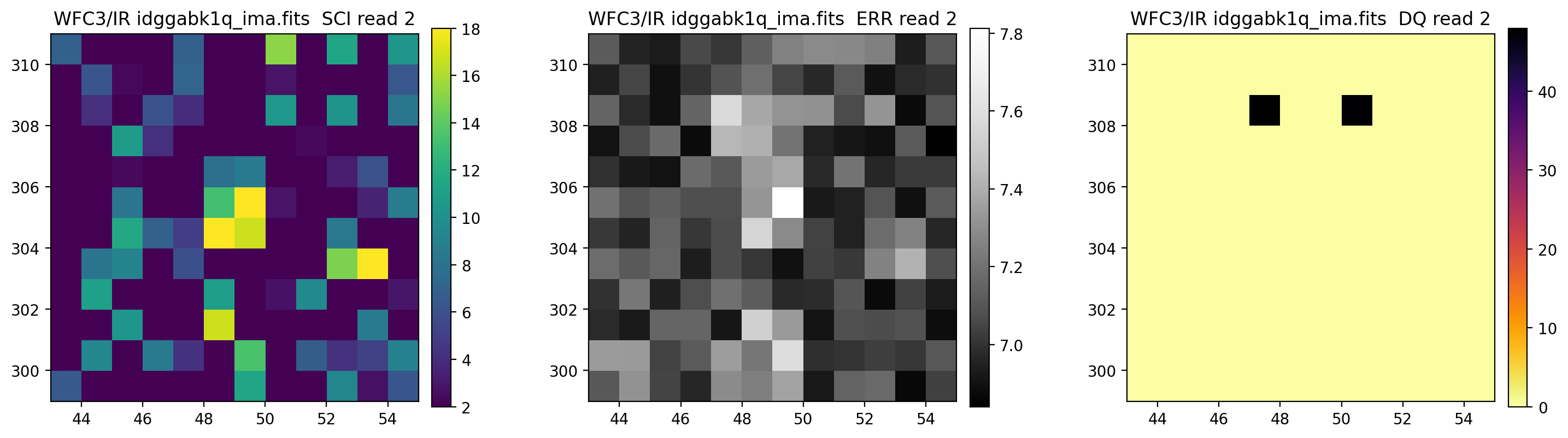
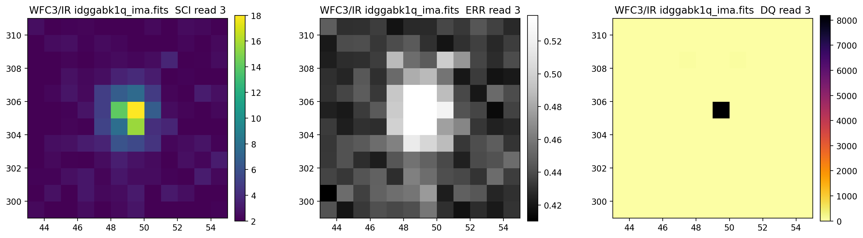
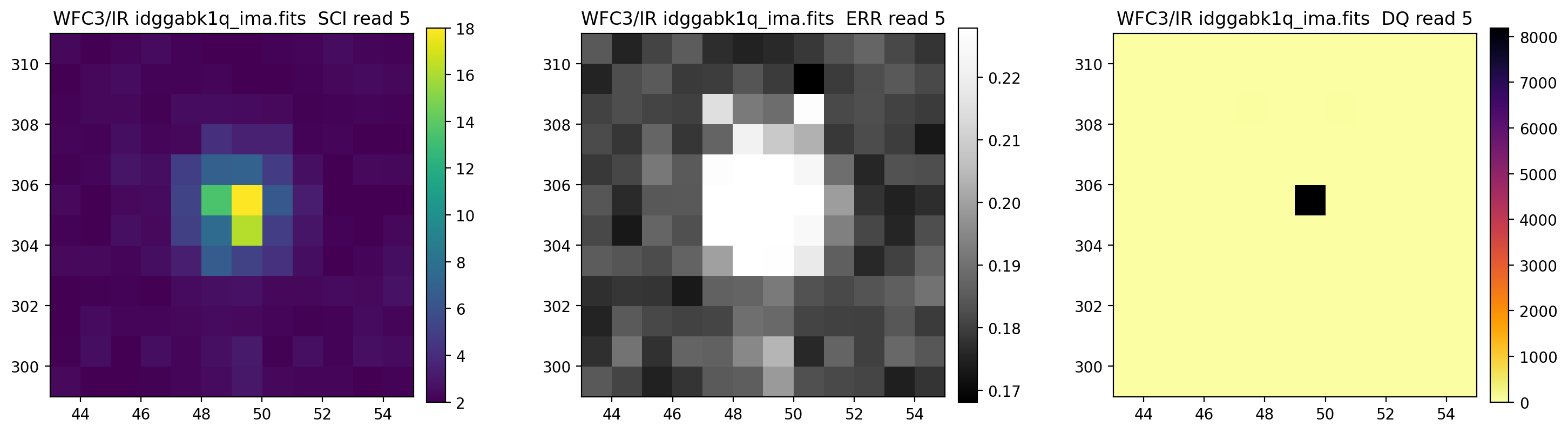
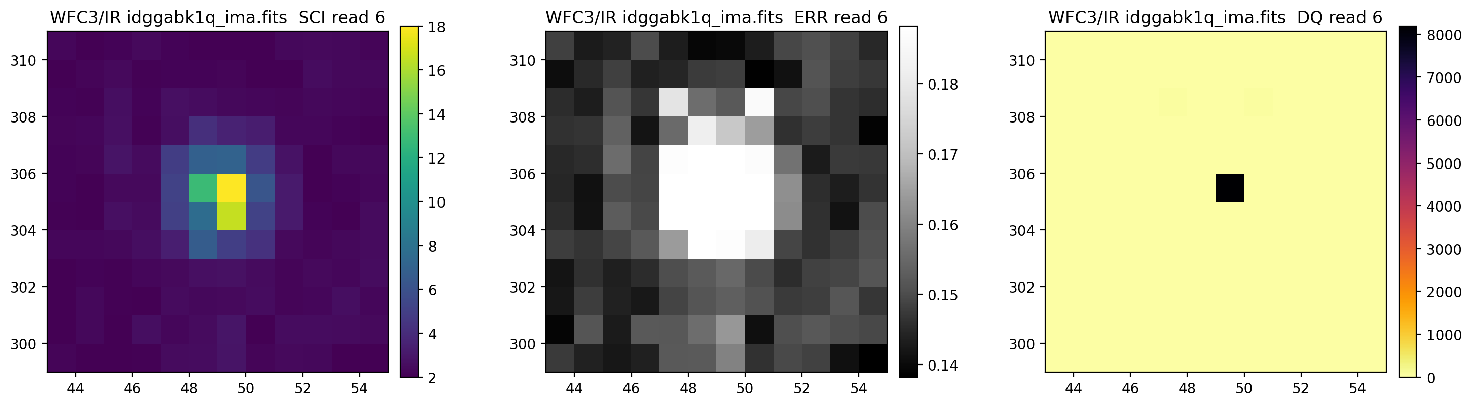
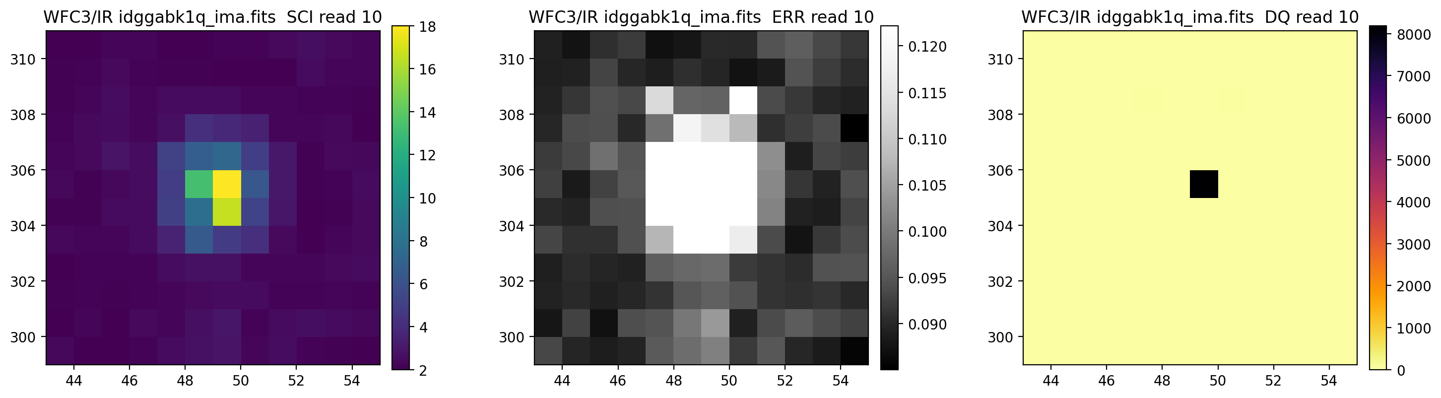
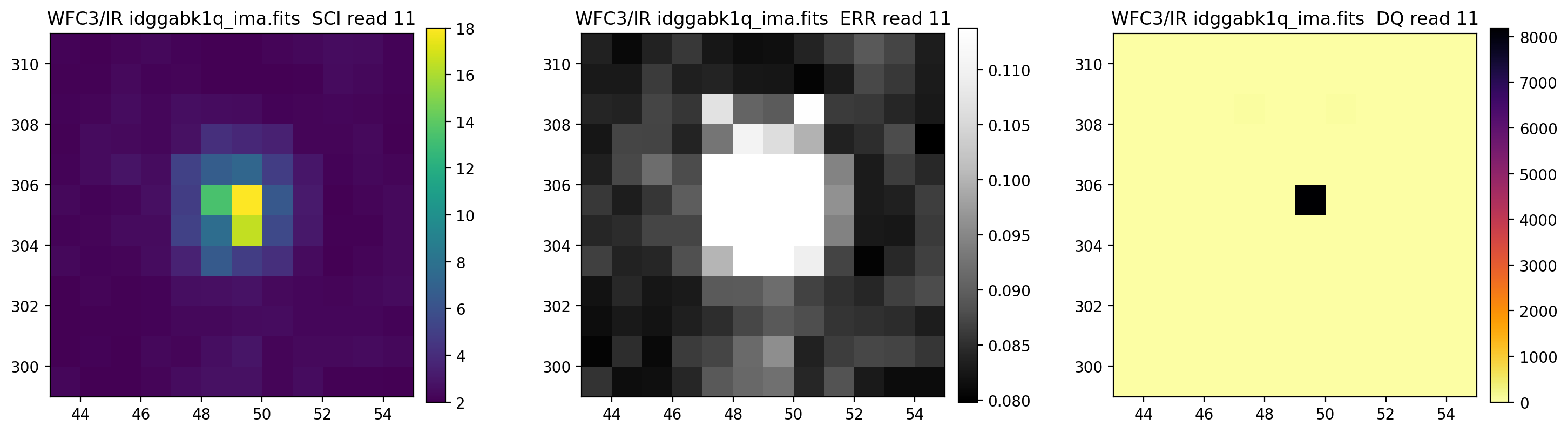
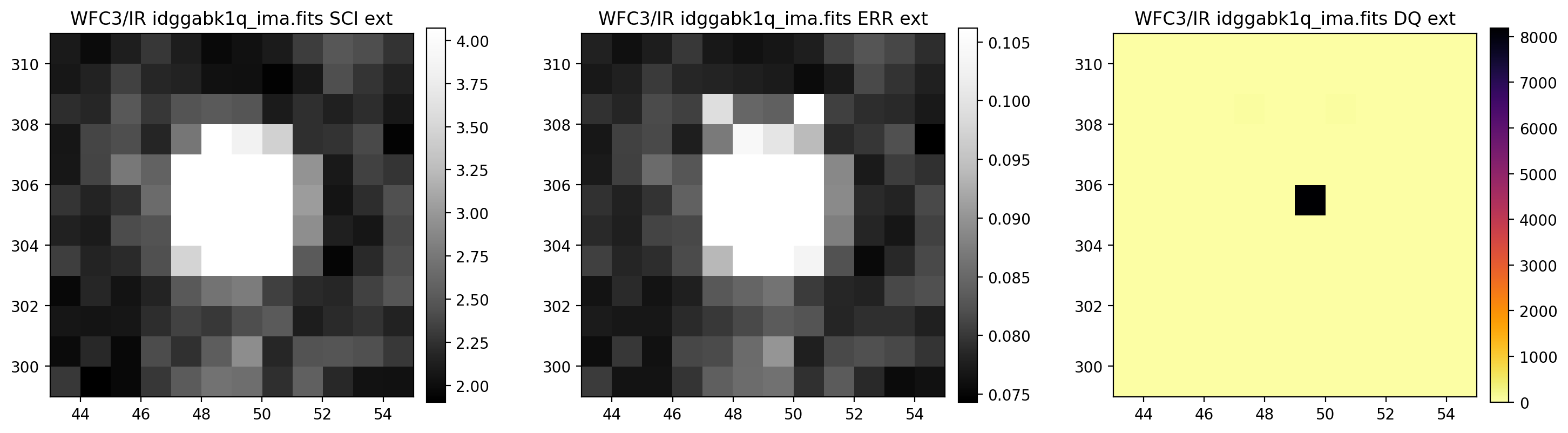
3.5 Display each read of ima image section#
In addition to changing each SCI array’s colormap and scaling, we display each read of the ima by setting ima_multiread=True.
display_image('idggabk1q_ima.fits[43:55,299:311]',
              colormaps=["viridis", "Greys_r", "inferno_r"],
              scaling=[(2, 18), (None, None), (None, None)],
              ima_multiread=True)


4. row_column_stats#
In this section, we demonstrate the functionality of row_column_stats, a useful tool for quickly computing WFC3 statistics.
The subsections explain how to compute row and column statistics for a full image, individual WFC3/UVIS chips, a section of
an image, and individual ima reads. The row/column numbers are on the x-axis and the statistics are on the y-axis.
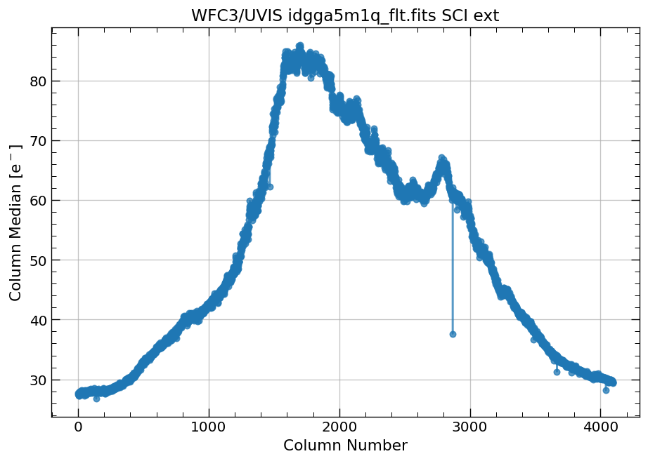
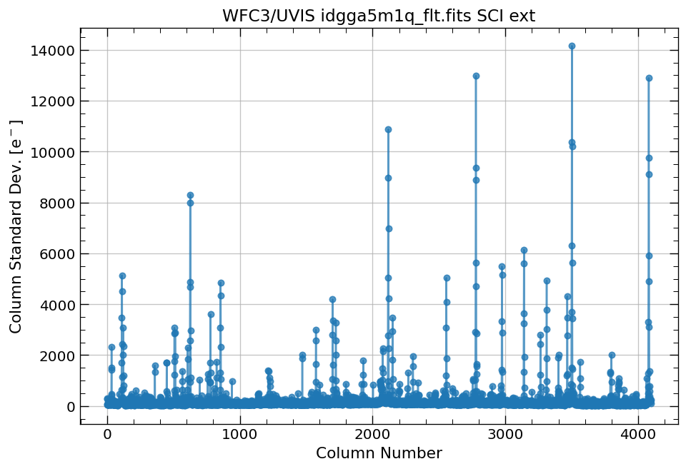
4.1 Compute column median and column standard deviation for a full image#
First, we plot the column median and standard deviations for our WFC3/UVIS image.
# plot column median for the full image
x, y = row_column_stats('idgga5m1q_flt.fits',
                        stat='median',
                        axis='column')

# plot column standard deviation for the full image
x, y = row_column_stats('idgga5m1q_flt.fits',
                        stat='stddev',
                        axis='column')
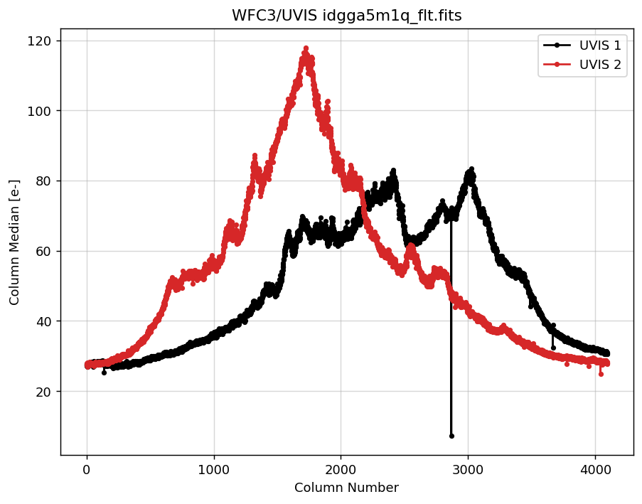
4.2 Measure UVIS1 & UVIS2 column medians separately and overplot on one figure#
Next, we plot the column medians for each individual WFC3/UVIS chip.
# get column median values for UVIS2 but don't plot
x2, y2 = row_column_stats('idgga5m1q_flt.fits[0:4096,0:2051]',
                          stat='median',
                          axis='column',
                          plot=False)

# get column median values for UVIS1 but don't plot
x1, y1 = row_column_stats('idgga5m1q_flt.fits[0:4096,2051:4102]',
                          stat='median',
                          axis='column',
                          plot=False)

# overplot UVIS1 and UVIS2 data on one figure
plt.figure(figsize=(8, 6), dpi=130)
plt.grid(alpha=.5)
plt.plot(x1, y1, marker='.', label='UVIS 1', color='k')
plt.plot(x2, y2, marker='.', label='UVIS 2', color='C3')
plt.title('WFC3/UVIS idgga5m1q_flt.fits')
plt.xlabel('Column Number')
plt.ylabel('Column Median [e-]')
plt.legend()
<matplotlib.legend.Legend at 0x7fa83983d490>
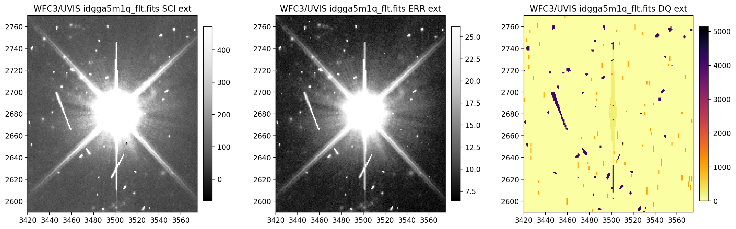
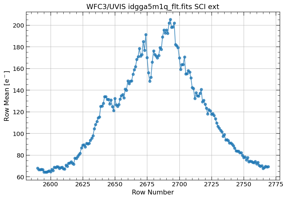
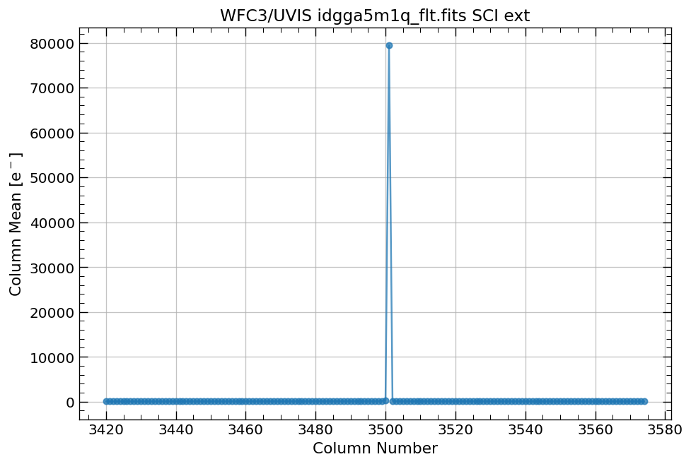
4.3 Display image section and compute row & column mean#
Now, we compute the row and column means for a section of our WFC3/UVIS image.
# Display a section of the image
display_image('idgga5m1q_flt.fits[3420:3575,2590:2770]')

# plot row mean for a section of the image
x, y = row_column_stats('idgga5m1q_flt.fits[3420:3575,2590:2770]',
                        stat='mean',
                        axis='row')

# plot column mean for a section of the image
x, y = row_column_stats('idgga5m1q_flt.fits[3420:3575,2590:2770]',
                        stat='mean',
                        axis='column')
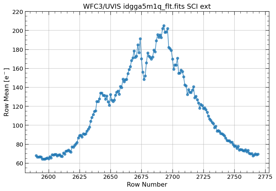
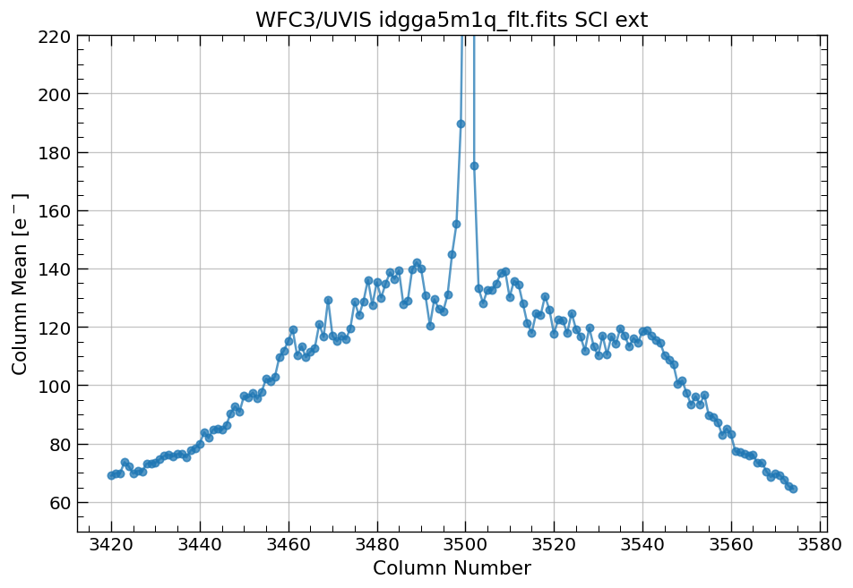
Note: Without specifying ylim, the y-axis limits (above) are set to matplotlib defaults.
Set ylim to (y1,y2) (below) to create custom y-axis limits from the previous example.
y1 = 50
y2 = 220

# Display a section of the image
display_image('idgga5m1q_flt.fits[3420:3575,2590:2770]')

# plot row mean for single source with custom yaxis limits
x, y = row_column_stats('idgga5m1q_flt.fits[3420:3575,2590:2770]',
                        stat='mean',
                        axis='row',
                        ylim=(y1, y2))

# plot column mean for single source with custom yaxis limits
x, y = row_column_stats('idgga5m1q_flt.fits[3420:3575,2590:2770]',
                        stat='mean',
                        axis='column',
                        ylim=(y1, y2))
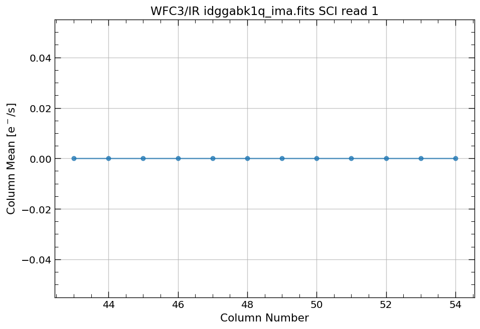
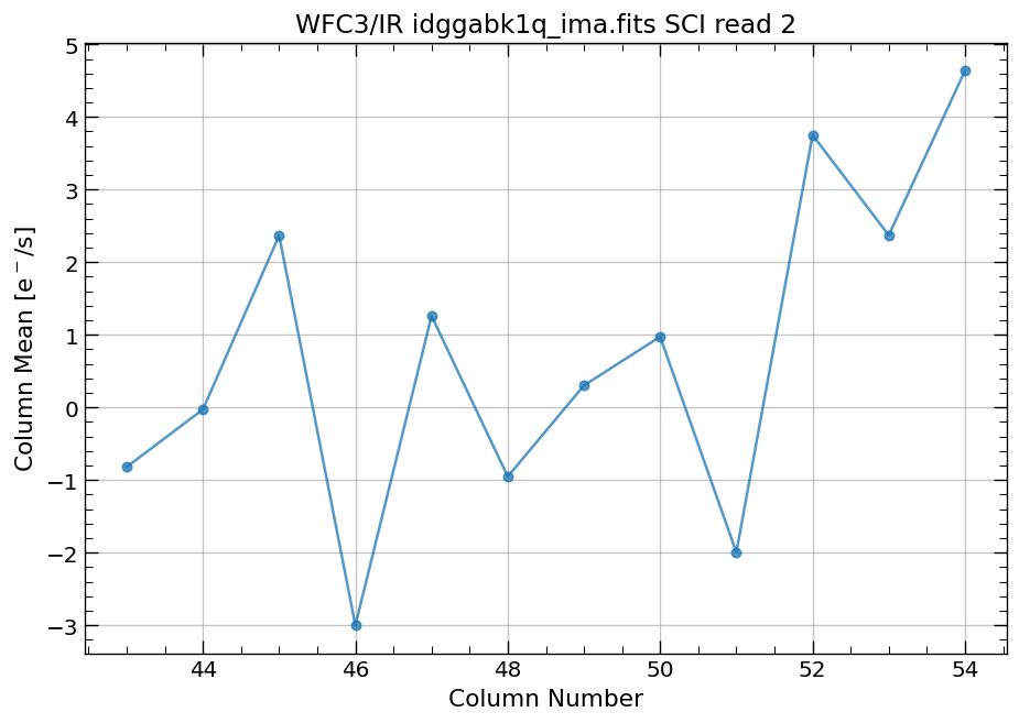
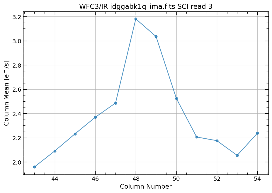
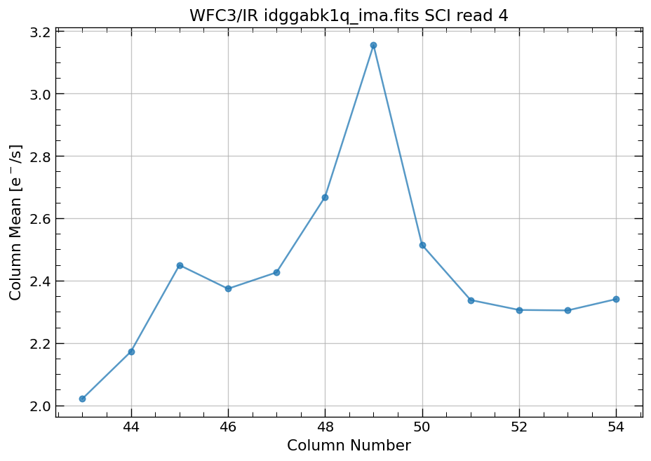
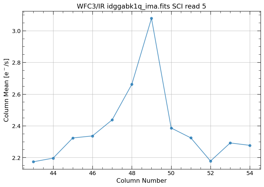
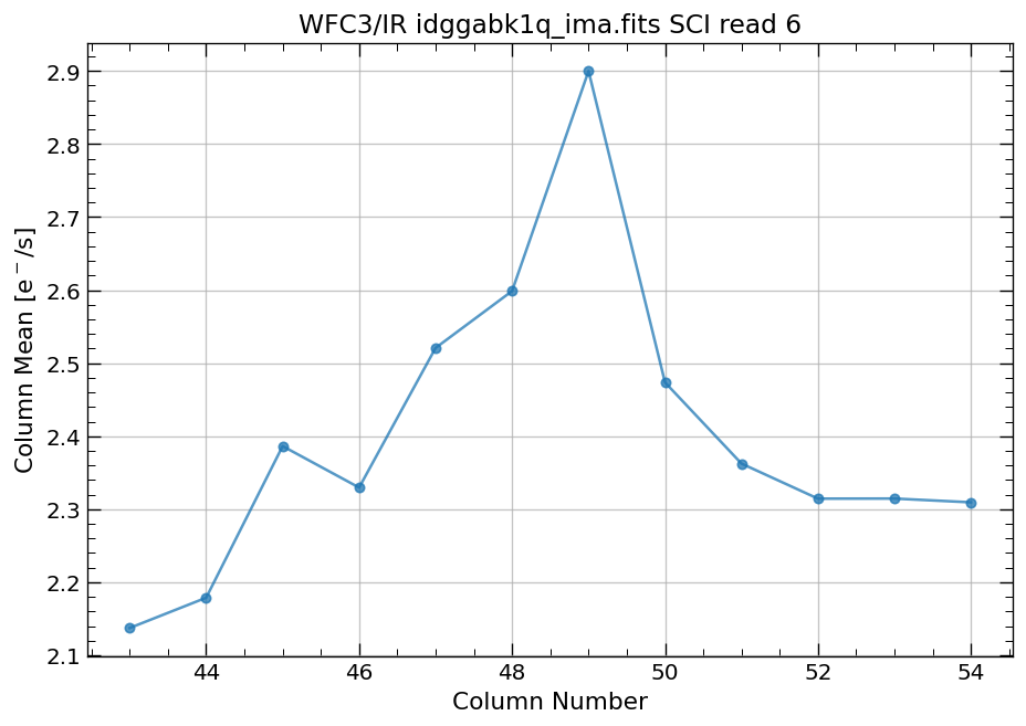
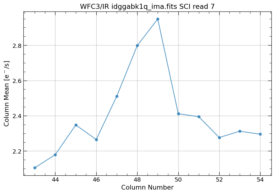
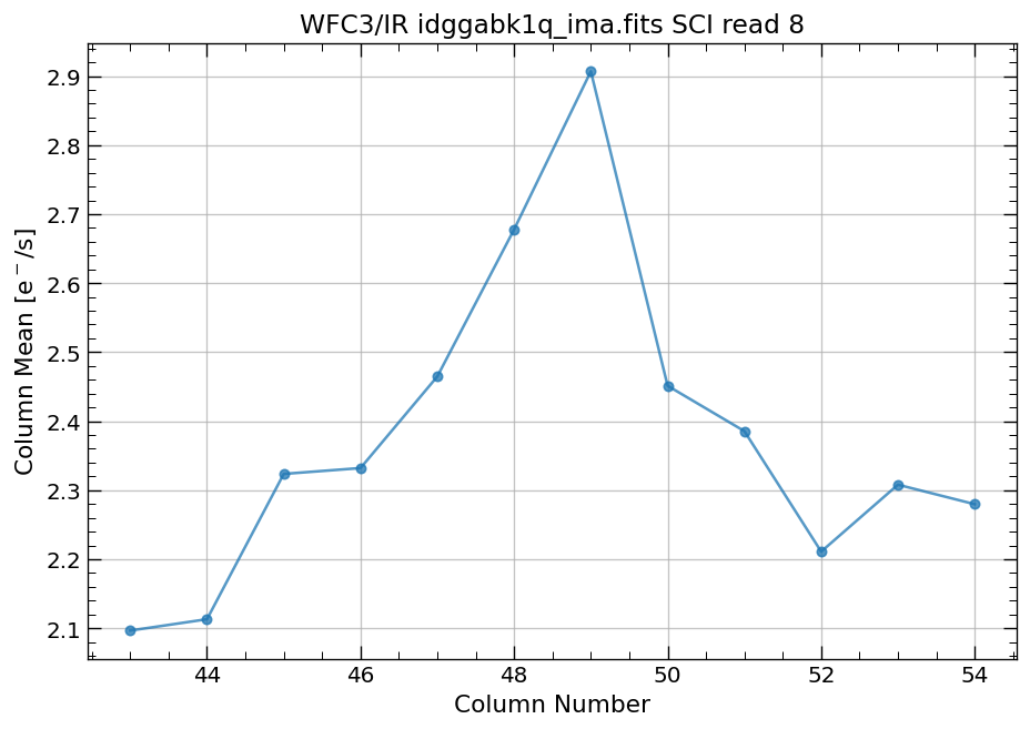
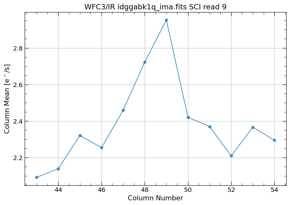
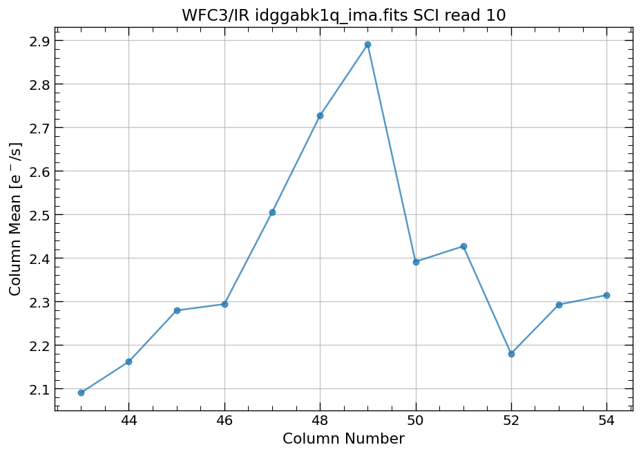
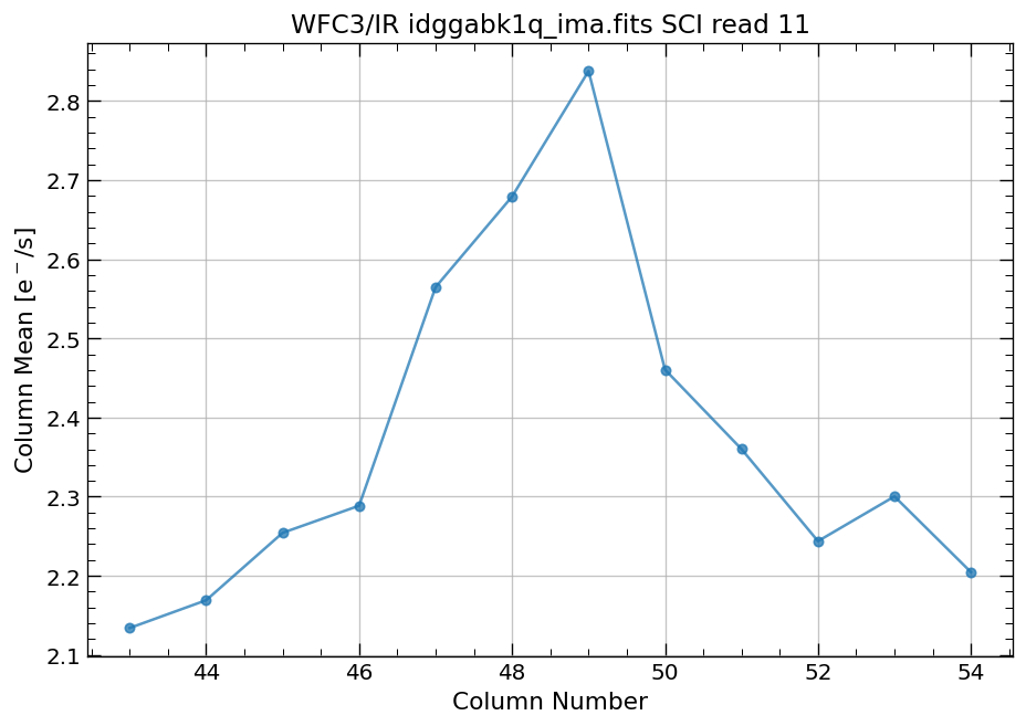
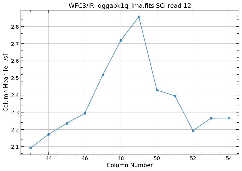
4.4 Compute column mean for each read of ima image section#
Finally, we compute the column means for the same section of each ima read.
# Display a section of the image
display_image('idggabk1q_ima.fits[43:55,299:311]')

# plot column mean for section of ima
x, y = row_column_stats('idggabk1q_ima.fits[43:55,299:311]',
                        stat='mean',
                        axis='column',
                        ima_multiread=True)
5. Conclusions#
Thank you for walking through this notebook. Now while analyzing WFC3 data, you should be more familiar with:
Using
display_imageto quickly inspect theSCI,ERR, andDQarrays of an image or image section.Using
row_column_statsto compute statistics on each individual column (or row) of an image or image section.
Congratulations, you have completed the notebook!#
Additional Resources#
Below are some additional resources that may be helpful. Please send any questions through the HST Helpdesk.
About this Notebook#
Author: Benjamin Kuhn; WFC3 Instrument Team
Updated on: 2021-10-04
Citations#
If you use numpy, matplotlib, astropy, or astroquery for published research, please cite the authors.
Follow these links for more information about citing the libraries below:
