Processing WFC3/UVIS Data with calwf3 Using the v1.0 CTE-Correction

Processing WFC3/UVIS Data with `calwf3` Using the v1.0 CTE-Correction#

Learning Goals#

This notebook explains how to calibrate raw WFC3/UVIS data with the v1.0 pixel-based CTE correction within calwf3.

By the end of this tutorial, you will:

Download a raw WFC3 image from MAST.
Find the necessary reference files needed for calibration.
Edit header keywords.
Run calwf3 v3.5.2 to calibrate the raw image with the v1.0 pixel based CTE-correction.
Compare v1.0 and v2.0 products.

Table of Contents#

Introduction

1. Imports
2. Verify archived_drkcfiles.txt is in CWD
3. Check that calwf3 Version is v3.5.2
4. Query MAST and Download a WFC3 raw.fits Image
5. Set CRDS Environment Variable and Download Reference Files
      5.1 Run crds bestrefs
      5.2 Inspect Image Header
6. Find the Correct v1.0 DRKCFILE
      6.1 Download the Correct DRKCFILE from CRDS
      6.2 Modify the Image Header Keyword, DRKCFILE
7. Download the v1.0 PCTETAB
      7.1 Modify the Image Header Keyword PCTETAB
8. Re-Inspect Image Header
9. Run calwf3
10. Inspect FLC Image Header
11. Investigate v1.0 and v2.0 Differences
      11.1 Download the v2.0 FLC File
      11.2 Open Files
      11.3 Display 50x50 Pixel Background Subsection
            11.3.1 Pixel Distribution of Background Subsections
      11.4 Display Image Subsection
      11.5 Aperture Photometry
12. Conclusions

Additional Resources
About the Notebook
Citations

Introduction#

The v1.0 pixel-based Charge Transfer Efficiency (CTE) correction was first implemented into calwf3 v3.3 in 2016
(Ryan et al. 2016, Anderson & Bedin 2010, HSTCAL release notes). This also marked the first time users could directly
download CTE-corrected flc & drc files from MAST. While the v1.0 correction was sufficient for many years, the
degradation of CTE over time reduced the efficacy of the model in treating low-level pixels. The v1.0 correction adversely
impacts (overcorrects) both the image background and faint sources. In April 2021 the v2.0 pixel-based CTE correction
was implemented in calwf3 v3.6.0 (Anderson et al. 2021, Kuhn & Anderson 2021, HSTCAL release notes). Since
MAST uses the latest release of calwf3 for calibration, any WFC3/UVIS CTE corrected data retrieved from MAST,
regardless of observation date, will be calibrated with the v2.0 pixel-based CTE correction. Although v1.0 pixel-based
CTE-corrected flc & drc files are no longer accessable through MAST, this notebook steps through the procedure
required to calibrate WFC3/UVIS images using the v1.0 CTE correction.

One of the limiting factors of using the v1.0 CTE correction are the CTE corrected dark current reference files (DRKCFILE).
These dark reference files are delivered to MAST by the WFC3 team and use the same pixel-based CTE correction within
calwf3. Now that we have switched to the v2.0 CTE correction there is a cut off for dark current reference files that use
the v1.0 correction. Observations taken after February 2021 will not have CTE corrected dark files using the v1.0 algorithm,
which means applying the v1.0 CTE correction works best for observations taken between May 2009 - February 2021.
If the observation being calibrated was taken after February 2021 there are two options: 1) use the last v1.0 CTE corrected
dark reference file from February 2021 or 2) use the v2.0 CTE corrected dark with the most appropriate USEAFTER for the
science exposure’s observation date.

1. Imports#

This notebook assumes you have created and activated a virtual environment using the requirements file in this notebook's repository. Please make sure you have read the README file before continuing.

We import:

Package Name	Purpose
`glob`	creating list of files
`os`	directory maintenance and setting environment variables
`astropy.io.fits`	opening and modifying fits files
`astroquery.mast.Observations`	downloading data from MAST
`astropy.table.Table`	creating and manipulating data tables
`astropy.visualization.ZScaleInterval`	finding z-scale limits when displaying images
`matplotlib.pyplot`	plotting and displaying images
`numpy`	finding indices and concatenating arrays
`photutils.aperture.aperture_photometry`	performing aperture photometry
`photutils.aperture.CircularAperture`	creating circular apertures
`photutils.aperture.CircularAnnulus`	creating circular annuli
`wfc3tools.calwf3`	verifying the version and running pipeline
`background_median.aperture_stats_tbl`	measuring background values within annuli

import glob
import os

from astropy.io import fits
from astropy.table import Table
from astroquery.mast import Observations
from astropy.visualization import ZScaleInterval
import matplotlib.pyplot as plt
import numpy as np
from photutils.aperture import aperture_photometry, CircularAperture, CircularAnnulus
from wfc3tools import calwf3

from example.background_median import aperture_stats_tbl

2. Verify `archived_drkcfiles.txt` is in CWD#

When you cloned/downloaded this notebook from hst_notebooks, a .txt file should have been included. The file name is
archived_drkcfiles.txt and it is used later on in the notebook. This .txt file includes the file name, delivery date, activation
date, and USEAFTER date for every v1.0 CTE corrected dark reference file between May 2009 - February 2021. Below, we will use
this file in conjunction with the observation date of the file(s) being calibrated to pick out the most appropriate v1.0 CTE corrected
dark reference file(s).

Please make sure the archived_drkcfiles.txt file is in the current working directory before continuing.

# list cwd to verify txt file is there
!ls -l archived_drkcfiles.txt

-rw-r--r-- 1 runner docker 350644 Nov 12 01:56 archived_drkcfiles.txt

3. Check that `calwf3` Version is `v3.5.2`#

In April 2021, a new calwf3 version was released that contains the v2.0 CTE-correction. If you would like to use the v1.0 correction, your
current environment must be using calwf3 versions equal to or between 3.3 - 3.5.2. However, in order to get the best v1.0 calibrated
images we must use calwf3 v3.5.2. This version of calwf3 includes the recent (~Jan 2021) update that added MJD as a parameterized
variable for the PHOTMODE keyword, which enables a time-dependent photometric correction and zeropoint. If your version is 3.6.0 or higher,
you must downgrade the hstcal package. The safer option, however, is to create a new environment using the requirements file provided in
the notebook’s repository:

$ conda config --add channels http://ssb.stsci.edu/astroconda
$ conda create -n v1_PCTE hstcal==2.5.0 python=3.11
$ conda activate v1_PCTE
$ pip install -r requirements.txt

hstcal v2.5.0 provides version 3.5.2 of calwf3, which is the last version that offers the v1.0 pixel-based CTE correction.

# print calwf3 version to make sure its equal to or between 3.3 and 3.5.2 
!calwf3.e --version

3.7.1

4. Query MAST and Download a WFC3 `raw.fits` Image#

Here, we download our image via astroquery. For more information, please look at the documentation for Astroquery, Astroquery.mast, and
CAOM Field Descriptions, which is used for the obs_table variable below. Additionally, you may download the data from MAST using either
the HST MAST Search Engine or the more general MAST Portal.

We download a raw image of star cluster 47 Tucanae (47Tuc, NGC 104), offset from the core, from CAL proposal 15576 (July 2019).
After downloading the image, we move it to the current working directory (cwd).

# Edit this cell's first line if you would to download your own file(s)
# Get the observation records
obs_table = Observations.query_criteria(obs_id='idv404axq*', proposal_id=15576)

# Get the listing of data products
products = Observations.get_product_list(obs_table)

# Filter the products for the RAW files
filtered_products = Observations.filter_products(products, productSubGroupDescription='RAW')

# Download all the images above
download_table = Observations.download_products(filtered_products, mrp_only=False)

# For convenience move raws to cwd and remove empty download dir
for file in download_table['Local Path']:
    filename = file.split('/')[-1]
    os.rename(file, os.path.basename(file))
    os.rmdir('mastDownload/HST/'+filename[:9])
        
os.rmdir('mastDownload/HST/')
os.rmdir('mastDownload/')

Downloading URL https://mast.stsci.edu/api/v0.1/Download/file?uri=mast:HST/product/idv404axq_raw.fits to ./mastDownload/HST/idv404axq/idv404axq_raw.fits ...

 [Done]

# show list of current dir to verify fits file is there
!ls -l *raw.fits

-rw-r--r-- 1 runner docker 34891200 Nov 12 01:57 idv404axq_raw.fits

5. Set CRDS Environment Variable and Download Reference Files#

If you already have the absolute paths set for CRDS, please skip the code cell immediately below and proceed to the crds bestrefs command in Section 5.1.

Before we run crds bestfefs and calwf3, we need to set environment variables for several subsequent calibration tasks. We will point to a
subdirectory within the main crds_cache/ using the IREF environment variable. The IREF variable is used for WFC3 reference files. Other
instruments use other variables, e.g., JREF for ACS. You have the option to permanently add these environment variables to your user profile by
adding the path in your shell’s configuration file. If you’re using bash, you would edit the ~/.bash_profile file with lines such as:

export CRDS_SERVER_URL="https://hst-crds.stsci.edu"
export CRDS_SERVER="https://hst-crds.stsci.edu"
export CRDS_PATH="$HOME/crds_cache"
export iref="${CRDS_PATH}/references/hst/wfc3/"

os.environ['CRDS_SERVER_URL'] = 'https://hst-crds.stsci.edu'
os.environ['CRDS_SERVER'] = 'https://hst-crds.stsci.edu'
os.environ['CRDS_PATH'] = 'crds_cache'
os.environ['iref'] = 'crds_cache/references/hst/wfc3/'

5.1 Run `crds bestrefs`#

The cell below calls CRDS bestref, which will copy the necessary reference files from CRDS over to your local machine, if you do not already have
them. Without running this command we would not be able to calibrate the image with calwf3.

!crds bestrefs --update-bestrefs --sync-references=1 --files idv404axq_raw.fits

CRDS - INFO -  Fetching  crds_cache/mappings/hst/hst_wfpc2_wf4tfile_0250.rmap         678 bytes  (1 / 142 files) (0 / 1.8 M bytes)

CRDS - INFO -  Fetching  crds_cache/mappings/hst/hst_wfpc2_shadfile_0250.rmap         977 bytes  (2 / 142 files) (678 / 1.8 M bytes)

CRDS - INFO -  Fetching  crds_cache/mappings/hst/hst_wfpc2_offtab_0250.rmap           642 bytes  (3 / 142 files) (1.7 K / 1.8 M bytes)

CRDS - INFO -  Fetching  crds_cache/mappings/hst/hst_wfpc2_maskfile_0250.rmap         685 bytes  (4 / 142 files) (2.3 K / 1.8 M bytes)

CRDS - INFO -  Fetching  crds_cache/mappings/hst/hst_wfpc2_idctab_0250.rmap           696 bytes  (5 / 142 files) (3.0 K / 1.8 M bytes)

CRDS - INFO -  Fetching  crds_cache/mappings/hst/hst_wfpc2_flatfile_0250.rmap      30.0 K bytes  (6 / 142 files) (3.7 K / 1.8 M bytes)

CRDS - INFO -  Fetching  crds_cache/mappings/hst/hst_wfpc2_dgeofile_0250.rmap         801 bytes  (7 / 142 files) (33.7 K / 1.8 M bytes)

CRDS - INFO -  Fetching  crds_cache/mappings/hst/hst_wfpc2_darkfile_0250.rmap     178.4 K bytes  (8 / 142 files) (34.5 K / 1.8 M bytes)

CRDS - INFO -  Fetching  crds_cache/mappings/hst/hst_wfpc2_biasfile_0250.rmap       3.3 K bytes  (9 / 142 files) (212.8 K / 1.8 M bytes)

CRDS - INFO -  Fetching  crds_cache/mappings/hst/hst_wfpc2_atodfile_0250.rmap         874 bytes  (10 / 142 files) (216.1 K / 1.8 M bytes)

CRDS - INFO -  Fetching  crds_cache/mappings/hst/hst_wfpc2_0250.imap                  782 bytes  (11 / 142 files) (217.0 K / 1.8 M bytes)

CRDS - INFO -  Fetching  crds_cache/mappings/hst/hst_wfc3_snkcfile_0003.rmap          681 bytes  (12 / 142 files) (217.8 K / 1.8 M bytes)

CRDS - INFO -  Fetching  crds_cache/mappings/hst/hst_wfc3_satufile_0002.rmap        1.0 K bytes  (13 / 142 files) (218.5 K / 1.8 M bytes)

CRDS - INFO -  Fetching  crds_cache/mappings/hst/hst_wfc3_pfltfile_0253.rmap       34.2 K bytes  (14 / 142 files) (219.5 K / 1.8 M bytes)

CRDS - INFO -  Fetching  crds_cache/mappings/hst/hst_wfc3_pctetab_0004.rmap           698 bytes  (15 / 142 files) (253.7 K / 1.8 M bytes)

CRDS - INFO -  Fetching  crds_cache/mappings/hst/hst_wfc3_oscntab_0250.rmap           747 bytes  (16 / 142 files) (254.4 K / 1.8 M bytes)

CRDS - INFO -  Fetching  crds_cache/mappings/hst/hst_wfc3_npolfile_0254.rmap        4.0 K bytes  (17 / 142 files) (255.1 K / 1.8 M bytes)

CRDS - INFO -  Fetching  crds_cache/mappings/hst/hst_wfc3_nlinfile_0250.rmap          726 bytes  (18 / 142 files) (259.2 K / 1.8 M bytes)

CRDS - INFO -  Fetching  crds_cache/mappings/hst/hst_wfc3_mdriztab_0254.rmap          845 bytes  (19 / 142 files) (259.9 K / 1.8 M bytes)

CRDS - INFO -  Fetching  crds_cache/mappings/hst/hst_wfc3_imphttab_0256.rmap          683 bytes  (20 / 142 files) (260.7 K / 1.8 M bytes)

CRDS - INFO -  Fetching  crds_cache/mappings/hst/hst_wfc3_idctab_0254.rmap            661 bytes  (21 / 142 files) (261.4 K / 1.8 M bytes)

CRDS - INFO -  Fetching  crds_cache/mappings/hst/hst_wfc3_flshfile_0256.rmap        5.8 K bytes  (22 / 142 files) (262.1 K / 1.8 M bytes)

CRDS - INFO -  Fetching  crds_cache/mappings/hst/hst_wfc3_drkcfile_0196.rmap      237.6 K bytes  (23 / 142 files) (267.9 K / 1.8 M bytes)

CRDS - INFO -  Fetching  crds_cache/mappings/hst/hst_wfc3_dfltfile_0002.rmap       17.1 K bytes  (24 / 142 files) (505.5 K / 1.8 M bytes)

CRDS - INFO -  Fetching  crds_cache/mappings/hst/hst_wfc3_darkfile_0495.rmap      284.9 K bytes  (25 / 142 files) (522.6 K / 1.8 M bytes)

CRDS - INFO -  Fetching  crds_cache/mappings/hst/hst_wfc3_d2imfile_0251.rmap          605 bytes  (26 / 142 files) (807.5 K / 1.8 M bytes)

CRDS - INFO -  Fetching  crds_cache/mappings/hst/hst_wfc3_crrejtab_0250.rmap          803 bytes  (27 / 142 files) (808.1 K / 1.8 M bytes)

CRDS - INFO -  Fetching  crds_cache/mappings/hst/hst_wfc3_ccdtab_0250.rmap            799 bytes  (28 / 142 files) (808.9 K / 1.8 M bytes)

CRDS - INFO -  Fetching  crds_cache/mappings/hst/hst_wfc3_bpixtab_0312.rmap        11.8 K bytes  (29 / 142 files) (809.7 K / 1.8 M bytes)

CRDS - INFO -  Fetching  crds_cache/mappings/hst/hst_wfc3_biasfile_0267.rmap       23.4 K bytes  (30 / 142 files) (821.5 K / 1.8 M bytes)

CRDS - INFO -  Fetching  crds_cache/mappings/hst/hst_wfc3_biacfile_0003.rmap          692 bytes  (31 / 142 files) (844.9 K / 1.8 M bytes)

CRDS - INFO -  Fetching  crds_cache/mappings/hst/hst_wfc3_atodtab_0250.rmap           651 bytes  (32 / 142 files) (845.6 K / 1.8 M bytes)

CRDS - INFO -  Fetching  crds_cache/mappings/hst/hst_wfc3_0600.imap                 1.3 K bytes  (33 / 142 files) (846.2 K / 1.8 M bytes)

CRDS - INFO -  Fetching  crds_cache/mappings/hst/hst_synphot_tmttab_0002.rmap         745 bytes  (34 / 142 files) (847.5 K / 1.8 M bytes)

CRDS - INFO -  Fetching  crds_cache/mappings/hst/hst_synphot_tmgtab_0012.rmap         767 bytes  (35 / 142 files) (848.3 K / 1.8 M bytes)

CRDS - INFO -  Fetching  crds_cache/mappings/hst/hst_synphot_tmctab_0055.rmap         743 bytes  (36 / 142 files) (849.0 K / 1.8 M bytes)

CRDS - INFO -  Fetching  crds_cache/mappings/hst/hst_synphot_thruput_0059.rmap    329.6 K bytes  (37 / 142 files) (849.8 K / 1.8 M bytes)

CRDS - INFO -  Fetching  crds_cache/mappings/hst/hst_synphot_thermal_0003.rmap     20.4 K bytes  (38 / 142 files) (1.2 M / 1.8 M bytes)

CRDS - INFO -  Fetching  crds_cache/mappings/hst/hst_synphot_obsmodes_0004.rmap       743 bytes  (39 / 142 files) (1.2 M / 1.8 M bytes)

CRDS - INFO -  Fetching  crds_cache/mappings/hst/hst_synphot_0070.imap                579 bytes  (40 / 142 files) (1.2 M / 1.8 M bytes)

CRDS - INFO -  Fetching  crds_cache/mappings/hst/hst_stis_xtractab_0250.rmap          815 bytes  (41 / 142 files) (1.2 M / 1.8 M bytes)

CRDS - INFO -  Fetching  crds_cache/mappings/hst/hst_stis_wcptab_0251.rmap            578 bytes  (42 / 142 files) (1.2 M / 1.8 M bytes)

CRDS - INFO -  Fetching  crds_cache/mappings/hst/hst_stis_teltab_0250.rmap            745 bytes  (43 / 142 files) (1.2 M / 1.8 M bytes)

CRDS - INFO -  Fetching  crds_cache/mappings/hst/hst_stis_tdstab_0254.rmap            921 bytes  (44 / 142 files) (1.2 M / 1.8 M bytes)

CRDS - INFO -  Fetching  crds_cache/mappings/hst/hst_stis_tdctab_0252.rmap            650 bytes  (45 / 142 files) (1.2 M / 1.8 M bytes)

CRDS - INFO -  Fetching  crds_cache/mappings/hst/hst_stis_srwtab_0250.rmap            745 bytes  (46 / 142 files) (1.2 M / 1.8 M bytes)

CRDS - INFO -  Fetching  crds_cache/mappings/hst/hst_stis_sptrctab_0251.rmap          895 bytes  (47 / 142 files) (1.2 M / 1.8 M bytes)

CRDS - INFO -  Fetching  crds_cache/mappings/hst/hst_stis_sdctab_0251.rmap            889 bytes  (48 / 142 files) (1.2 M / 1.8 M bytes)

CRDS - INFO -  Fetching  crds_cache/mappings/hst/hst_stis_riptab_0254.rmap            877 bytes  (49 / 142 files) (1.2 M / 1.8 M bytes)

CRDS - INFO -  Fetching  crds_cache/mappings/hst/hst_stis_phottab_0258.rmap         1.6 K bytes  (50 / 142 files) (1.2 M / 1.8 M bytes)

CRDS - INFO -  Fetching  crds_cache/mappings/hst/hst_stis_pfltfile_0250.rmap       23.7 K bytes  (51 / 142 files) (1.2 M / 1.8 M bytes)

CRDS - INFO -  Fetching  crds_cache/mappings/hst/hst_stis_pctab_0250.rmap           3.1 K bytes  (52 / 142 files) (1.2 M / 1.8 M bytes)

CRDS - INFO -  Fetching  crds_cache/mappings/hst/hst_stis_mofftab_0250.rmap           747 bytes  (53 / 142 files) (1.2 M / 1.8 M bytes)

CRDS - INFO -  Fetching  crds_cache/mappings/hst/hst_stis_mlintab_0250.rmap           601 bytes  (54 / 142 files) (1.2 M / 1.8 M bytes)

CRDS - INFO -  Fetching  crds_cache/mappings/hst/hst_stis_lfltfile_0250.rmap       11.8 K bytes  (55 / 142 files) (1.2 M / 1.8 M bytes)

CRDS - INFO -  Fetching  crds_cache/mappings/hst/hst_stis_lamptab_0250.rmap           610 bytes  (56 / 142 files) (1.2 M / 1.8 M bytes)

CRDS - INFO -  Fetching  crds_cache/mappings/hst/hst_stis_inangtab_0250.rmap          815 bytes  (57 / 142 files) (1.3 M / 1.8 M bytes)

CRDS - INFO -  Fetching  crds_cache/mappings/hst/hst_stis_imphttab_0252.rmap          616 bytes  (58 / 142 files) (1.3 M / 1.8 M bytes)

CRDS - INFO -  Fetching  crds_cache/mappings/hst/hst_stis_idctab_0251.rmap            775 bytes  (59 / 142 files) (1.3 M / 1.8 M bytes)

CRDS - INFO -  Fetching  crds_cache/mappings/hst/hst_stis_halotab_0250.rmap           747 bytes  (60 / 142 files) (1.3 M / 1.8 M bytes)

CRDS - INFO -  Fetching  crds_cache/mappings/hst/hst_stis_gactab_0250.rmap            651 bytes  (61 / 142 files) (1.3 M / 1.8 M bytes)

CRDS - INFO -  Fetching  crds_cache/mappings/hst/hst_stis_exstab_0250.rmap            745 bytes  (62 / 142 files) (1.3 M / 1.8 M bytes)

CRDS - INFO -  Fetching  crds_cache/mappings/hst/hst_stis_echsctab_0250.rmap          749 bytes  (63 / 142 files) (1.3 M / 1.8 M bytes)

CRDS - INFO -  Fetching  crds_cache/mappings/hst/hst_stis_disptab_0250.rmap           813 bytes  (64 / 142 files) (1.3 M / 1.8 M bytes)

CRDS - INFO -  Fetching  crds_cache/mappings/hst/hst_stis_darkfile_0355.rmap       60.1 K bytes  (65 / 142 files) (1.3 M / 1.8 M bytes)

CRDS - INFO -  Fetching  crds_cache/mappings/hst/hst_stis_crrejtab_0250.rmap          711 bytes  (66 / 142 files) (1.3 M / 1.8 M bytes)

CRDS - INFO -  Fetching  crds_cache/mappings/hst/hst_stis_cdstab_0250.rmap            745 bytes  (67 / 142 files) (1.3 M / 1.8 M bytes)

CRDS - INFO -  Fetching  crds_cache/mappings/hst/hst_stis_ccdtab_0252.rmap            893 bytes  (68 / 142 files) (1.3 M / 1.8 M bytes)

CRDS - INFO -  Fetching  crds_cache/mappings/hst/hst_stis_bpixtab_0250.rmap           845 bytes  (69 / 142 files) (1.3 M / 1.8 M bytes)

CRDS - INFO -  Fetching  crds_cache/mappings/hst/hst_stis_biasfile_0357.rmap      120.2 K bytes  (70 / 142 files) (1.3 M / 1.8 M bytes)

CRDS - INFO -  Fetching  crds_cache/mappings/hst/hst_stis_apertab_0250.rmap           588 bytes  (71 / 142 files) (1.4 M / 1.8 M bytes)

CRDS - INFO -  Fetching  crds_cache/mappings/hst/hst_stis_apdestab_0252.rmap          636 bytes  (72 / 142 files) (1.4 M / 1.8 M bytes)

CRDS - INFO -  Fetching  crds_cache/mappings/hst/hst_stis_0371.imap                 1.7 K bytes  (73 / 142 files) (1.4 M / 1.8 M bytes)

CRDS - INFO -  Fetching  crds_cache/mappings/hst/hst_nicmos_zprattab_0250.rmap        646 bytes  (74 / 142 files) (1.4 M / 1.8 M bytes)

CRDS - INFO -  Fetching  crds_cache/mappings/hst/hst_nicmos_tempfile_0250.rmap      1.1 K bytes  (75 / 142 files) (1.4 M / 1.8 M bytes)

CRDS - INFO -  Fetching  crds_cache/mappings/hst/hst_nicmos_tdffile_0250.rmap       8.9 K bytes  (76 / 142 files) (1.4 M / 1.8 M bytes)

CRDS - INFO -  Fetching  crds_cache/mappings/hst/hst_nicmos_saadfile_0250.rmap        771 bytes  (77 / 142 files) (1.5 M / 1.8 M bytes)

CRDS - INFO -  Fetching  crds_cache/mappings/hst/hst_nicmos_saacntab_0250.rmap        594 bytes  (78 / 142 files) (1.5 M / 1.8 M bytes)

CRDS - INFO -  Fetching  crds_cache/mappings/hst/hst_nicmos_rnlcortb_0250.rmap        771 bytes  (79 / 142 files) (1.5 M / 1.8 M bytes)

CRDS - INFO -  Fetching  crds_cache/mappings/hst/hst_nicmos_pmskfile_0250.rmap        603 bytes  (80 / 142 files) (1.5 M / 1.8 M bytes)

CRDS - INFO -  Fetching  crds_cache/mappings/hst/hst_nicmos_pmodfile_0250.rmap        603 bytes  (81 / 142 files) (1.5 M / 1.8 M bytes)

CRDS - INFO -  Fetching  crds_cache/mappings/hst/hst_nicmos_phottab_0250.rmap         862 bytes  (82 / 142 files) (1.5 M / 1.8 M bytes)

CRDS - INFO -  Fetching  crds_cache/mappings/hst/hst_nicmos_pedsbtab_0250.rmap        594 bytes  (83 / 142 files) (1.5 M / 1.8 M bytes)

CRDS - INFO -  Fetching  crds_cache/mappings/hst/hst_nicmos_noisfile_0250.rmap      2.6 K bytes  (84 / 142 files) (1.5 M / 1.8 M bytes)

CRDS - INFO -  Fetching  crds_cache/mappings/hst/hst_nicmos_nlinfile_0250.rmap      1.7 K bytes  (85 / 142 files) (1.5 M / 1.8 M bytes)

CRDS - INFO -  Fetching  crds_cache/mappings/hst/hst_nicmos_maskfile_0250.rmap      1.2 K bytes  (86 / 142 files) (1.5 M / 1.8 M bytes)

CRDS - INFO -  Fetching  crds_cache/mappings/hst/hst_nicmos_illmfile_0250.rmap      5.8 K bytes  (87 / 142 files) (1.5 M / 1.8 M bytes)

CRDS - INFO -  Fetching  crds_cache/mappings/hst/hst_nicmos_idctab_0250.rmap          767 bytes  (88 / 142 files) (1.5 M / 1.8 M bytes)

CRDS - INFO -  Fetching  crds_cache/mappings/hst/hst_nicmos_flatfile_0250.rmap     11.0 K bytes  (89 / 142 files) (1.5 M / 1.8 M bytes)

CRDS - INFO -  Fetching  crds_cache/mappings/hst/hst_nicmos_darkfile_0250.rmap     14.9 K bytes  (90 / 142 files) (1.5 M / 1.8 M bytes)

CRDS - INFO -  Fetching  crds_cache/mappings/hst/hst_nicmos_0250.imap               1.1 K bytes  (91 / 142 files) (1.5 M / 1.8 M bytes)

CRDS - INFO -  Fetching  crds_cache/mappings/hst/hst_cos_ywlkfile_0003.rmap           922 bytes  (92 / 142 files) (1.5 M / 1.8 M bytes)

CRDS - INFO -  Fetching  crds_cache/mappings/hst/hst_cos_xwlkfile_0002.rmap           922 bytes  (93 / 142 files) (1.5 M / 1.8 M bytes)

CRDS - INFO -  Fetching  crds_cache/mappings/hst/hst_cos_xtractab_0269.rmap         1.6 K bytes  (94 / 142 files) (1.5 M / 1.8 M bytes)

CRDS - INFO -  Fetching  crds_cache/mappings/hst/hst_cos_wcptab_0257.rmap           1.3 K bytes  (95 / 142 files) (1.5 M / 1.8 M bytes)

CRDS - INFO -  Fetching  crds_cache/mappings/hst/hst_cos_twozxtab_0277.rmap           990 bytes  (96 / 142 files) (1.5 M / 1.8 M bytes)

CRDS - INFO -  Fetching  crds_cache/mappings/hst/hst_cos_tracetab_0276.rmap           998 bytes  (97 / 142 files) (1.5 M / 1.8 M bytes)

CRDS - INFO -  Fetching  crds_cache/mappings/hst/hst_cos_tdstab_0272.rmap             803 bytes  (98 / 142 files) (1.5 M / 1.8 M bytes)

CRDS - INFO -  Fetching  crds_cache/mappings/hst/hst_cos_spwcstab_0255.rmap         1.1 K bytes  (99 / 142 files) (1.5 M / 1.8 M bytes)

CRDS - INFO -  Fetching  crds_cache/mappings/hst/hst_cos_spottab_0006.rmap            766 bytes  (100 / 142 files) (1.5 M / 1.8 M bytes)

CRDS - INFO -  Fetching  crds_cache/mappings/hst/hst_cos_proftab_0276.rmap          1.0 K bytes  (101 / 142 files) (1.5 M / 1.8 M bytes)

CRDS - INFO -  Fetching  crds_cache/mappings/hst/hst_cos_phatab_0250.rmap             668 bytes  (102 / 142 files) (1.5 M / 1.8 M bytes)

CRDS - INFO -  Fetching  crds_cache/mappings/hst/hst_cos_lamptab_0264.rmap          1.4 K bytes  (103 / 142 files) (1.5 M / 1.8 M bytes)

CRDS - INFO -  Fetching  crds_cache/mappings/hst/hst_cos_hvtab_0259.rmap              567 bytes  (104 / 142 files) (1.5 M / 1.8 M bytes)

CRDS - INFO -  Fetching  crds_cache/mappings/hst/hst_cos_hvdstab_0002.rmap          1.0 K bytes  (105 / 142 files) (1.5 M / 1.8 M bytes)

CRDS - INFO -  Fetching  crds_cache/mappings/hst/hst_cos_gsagtab_0261.rmap            712 bytes  (106 / 142 files) (1.5 M / 1.8 M bytes)

CRDS - INFO -  Fetching  crds_cache/mappings/hst/hst_cos_geofile_0250.rmap            670 bytes  (107 / 142 files) (1.5 M / 1.8 M bytes)

CRDS - INFO -  Fetching  crds_cache/mappings/hst/hst_cos_fluxtab_0282.rmap          1.7 K bytes  (108 / 142 files) (1.5 M / 1.8 M bytes)

CRDS - INFO -  Fetching  crds_cache/mappings/hst/hst_cos_flatfile_0264.rmap         1.8 K bytes  (109 / 142 files) (1.5 M / 1.8 M bytes)

CRDS - INFO -  Fetching  crds_cache/mappings/hst/hst_cos_disptab_0276.rmap          1.7 K bytes  (110 / 142 files) (1.5 M / 1.8 M bytes)

CRDS - INFO -  Fetching  crds_cache/mappings/hst/hst_cos_dgeofile_0002.rmap           909 bytes  (111 / 142 files) (1.5 M / 1.8 M bytes)

CRDS - INFO -  Fetching  crds_cache/mappings/hst/hst_cos_deadtab_0250.rmap            711 bytes  (112 / 142 files) (1.5 M / 1.8 M bytes)

CRDS - INFO -  Fetching  crds_cache/mappings/hst/hst_cos_brsttab_0250.rmap            696 bytes  (113 / 142 files) (1.5 M / 1.8 M bytes)

CRDS - INFO -  Fetching  crds_cache/mappings/hst/hst_cos_brftab_0250.rmap             614 bytes  (114 / 142 files) (1.5 M / 1.8 M bytes)

CRDS - INFO -  Fetching  crds_cache/mappings/hst/hst_cos_bpixtab_0260.rmap            773 bytes  (115 / 142 files) (1.5 M / 1.8 M bytes)

CRDS - INFO -  Fetching  crds_cache/mappings/hst/hst_cos_badttab_0252.rmap            643 bytes  (116 / 142 files) (1.5 M / 1.8 M bytes)

CRDS - INFO -  Fetching  crds_cache/mappings/hst/hst_cos_0359.imap                  1.4 K bytes  (117 / 142 files) (1.5 M / 1.8 M bytes)

CRDS - INFO -  Fetching  crds_cache/mappings/hst/hst_acs_spottab_0251.rmap            641 bytes  (118 / 142 files) (1.5 M / 1.8 M bytes)

CRDS - INFO -  Fetching  crds_cache/mappings/hst/hst_acs_snkcfile_0100.rmap         7.5 K bytes  (119 / 142 files) (1.5 M / 1.8 M bytes)

CRDS - INFO -  Fetching  crds_cache/mappings/hst/hst_acs_shadfile_0251.rmap           531 bytes  (120 / 142 files) (1.5 M / 1.8 M bytes)

CRDS - INFO -  Fetching  crds_cache/mappings/hst/hst_acs_satufile_0002.rmap         1.2 K bytes  (121 / 142 files) (1.5 M / 1.8 M bytes)

CRDS - INFO -  Fetching  crds_cache/mappings/hst/hst_acs_pfltfile_0253.rmap        69.2 K bytes  (122 / 142 files) (1.5 M / 1.8 M bytes)

CRDS - INFO -  Fetching  crds_cache/mappings/hst/hst_acs_pctetab_0253.rmap            615 bytes  (123 / 142 files) (1.6 M / 1.8 M bytes)

CRDS - INFO -  Fetching  crds_cache/mappings/hst/hst_acs_oscntab_0251.rmap            781 bytes  (124 / 142 files) (1.6 M / 1.8 M bytes)

CRDS - INFO -  Fetching  crds_cache/mappings/hst/hst_acs_npolfile_0253.rmap         3.2 K bytes  (125 / 142 files) (1.6 M / 1.8 M bytes)

CRDS - INFO -  Fetching  crds_cache/mappings/hst/hst_acs_mlintab_0250.rmap            646 bytes  (126 / 142 files) (1.6 M / 1.8 M bytes)

CRDS - INFO -  Fetching  crds_cache/mappings/hst/hst_acs_mdriztab_0253.rmap           769 bytes  (127 / 142 files) (1.6 M / 1.8 M bytes)

CRDS - INFO -  Fetching  crds_cache/mappings/hst/hst_acs_imphttab_0260.rmap           769 bytes  (128 / 142 files) (1.6 M / 1.8 M bytes)

CRDS - INFO -  Fetching  crds_cache/mappings/hst/hst_acs_idctab_0256.rmap           1.5 K bytes  (129 / 142 files) (1.6 M / 1.8 M bytes)

CRDS - INFO -  Fetching  crds_cache/mappings/hst/hst_acs_flshfile_0268.rmap         3.4 K bytes  (130 / 142 files) (1.6 M / 1.8 M bytes)

CRDS - INFO -  Fetching  crds_cache/mappings/hst/hst_acs_drkcfile_0451.rmap        15.0 K bytes  (131 / 142 files) (1.6 M / 1.8 M bytes)

CRDS - INFO -  Fetching  crds_cache/mappings/hst/hst_acs_dgeofile_0250.rmap         3.2 K bytes  (132 / 142 files) (1.6 M / 1.8 M bytes)

CRDS - INFO -  Fetching  crds_cache/mappings/hst/hst_acs_darkfile_0442.rmap        87.0 K bytes  (133 / 142 files) (1.6 M / 1.8 M bytes)

CRDS - INFO -  Fetching  crds_cache/mappings/hst/hst_acs_d2imfile_0253.rmap           601 bytes  (134 / 142 files) (1.7 M / 1.8 M bytes)

CRDS - INFO -  Fetching  crds_cache/mappings/hst/hst_acs_crrejtab_0251.rmap           945 bytes  (135 / 142 files) (1.7 M / 1.8 M bytes)

CRDS - INFO -  Fetching  crds_cache/mappings/hst/hst_acs_cfltfile_0250.rmap         1.2 K bytes  (136 / 142 files) (1.7 M / 1.8 M bytes)

CRDS - INFO -  Fetching  crds_cache/mappings/hst/hst_acs_ccdtab_0256.rmap           1.4 K bytes  (137 / 142 files) (1.7 M / 1.8 M bytes)

CRDS - INFO -  Fetching  crds_cache/mappings/hst/hst_acs_bpixtab_0252.rmap          1.0 K bytes  (138 / 142 files) (1.7 M / 1.8 M bytes)

CRDS - INFO -  Fetching  crds_cache/mappings/hst/hst_acs_biasfile_0440.rmap        57.0 K bytes  (139 / 142 files) (1.7 M / 1.8 M bytes)

CRDS - INFO -  Fetching  crds_cache/mappings/hst/hst_acs_atodtab_0251.rmap            528 bytes  (140 / 142 files) (1.8 M / 1.8 M bytes)

CRDS - INFO -  Fetching  crds_cache/mappings/hst/hst_acs_0541.imap                  1.3 K bytes  (141 / 142 files) (1.8 M / 1.8 M bytes)

CRDS - INFO -  Fetching  crds_cache/mappings/hst/hst_1192.pmap                        495 bytes  (142 / 142 files) (1.8 M / 1.8 M bytes)

CRDS - INFO -  No comparison context or source comparison requested.

CRDS - INFO -  ===> Processing idv404axq_raw.fits

CRDS - INFO -  Fetching  crds_cache/references/hst/wfc3/2731450pi_idc.fits         40.3 K bytes  (1 / 18 files) (0 / 1.3 G bytes)

CRDS - INFO -  Fetching  crds_cache/references/hst/wfc3/27d1518pi_npl.fits         49.0 K bytes  (2 / 18 files) (40.3 K / 1.3 G bytes)

CRDS - INFO -  Fetching  crds_cache/references/hst/wfc3/2ck18260i_mdz.fits        118.1 K bytes  (3 / 18 files) (89.3 K / 1.3 G bytes)

CRDS - INFO -  Fetching  crds_cache/references/hst/wfc3/3a32019bi_bpx.fits          1.7 M bytes  (4 / 18 files) (207.4 K / 1.3 G bytes)

CRDS - INFO -  Fetching  crds_cache/references/hst/wfc3/42h2117di_bia.fits        174.2 M bytes  (5 / 18 files) (1.9 M / 1.3 G bytes)

CRDS - INFO -  Fetching  crds_cache/references/hst/wfc3/51c1638pi_imp.fits        397.4 K bytes  (6 / 18 files) (176.1 M / 1.3 G bytes)

CRDS - INFO -  Fetching  crds_cache/references/hst/wfc3/54l1347ei_cte.fits          1.2 M bytes  (7 / 18 files) (176.5 M / 1.3 G bytes)

CRDS - INFO -  Fetching  crds_cache/references/hst/wfc3/6c82013hi_fls.fits        209.0 M bytes  (8 / 18 files) (177.6 M / 1.3 G bytes)

CRDS - INFO -  Fetching  crds_cache/references/hst/wfc3/7b21735ti_sat.fits        174.2 M bytes  (9 / 18 files) (386.6 M / 1.3 G bytes)

CRDS - INFO -  Fetching  crds_cache/references/hst/wfc3/7bg1930ki_dkc.fits        168.1 M bytes  (10 / 18 files) (560.8 M / 1.3 G bytes)

CRDS - INFO -  Fetching  crds_cache/references/hst/wfc3/7bg1956fi_drk.fits        168.1 M bytes  (11 / 18 files) (728.9 M / 1.3 G bytes)

CRDS - INFO -  Fetching  crds_cache/references/hst/wfc3/n9i1435li_crr.fits         11.5 K bytes  (12 / 18 files) (897.0 M / 1.3 G bytes)

CRDS - INFO -  Fetching  crds_cache/references/hst/wfc3/q911321oi_osc.fits         25.9 K bytes  (13 / 18 files) (897.0 M / 1.3 G bytes)

CRDS - INFO -  Fetching  crds_cache/references/hst/wfc3/t291659mi_ccd.fits        247.7 K bytes  (14 / 18 files) (897.0 M / 1.3 G bytes)

CRDS - INFO -  Fetching  crds_cache/references/hst/wfc3/y7b1516hi_d2i.fits         51.8 K bytes  (15 / 18 files) (897.3 M / 1.3 G bytes)

CRDS - INFO -  Fetching  crds_cache/references/hst/wfc3/zcv20544i_pfl.fits        168.1 M bytes  (16 / 18 files) (897.3 M / 1.3 G bytes)

CRDS - INFO -  Fetching  crds_cache/references/hst/wfc3/zcv2057ni_bic.fits        174.2 M bytes  (17 / 18 files) (1.1 G / 1.3 G bytes)

CRDS - INFO -  Fetching  crds_cache/references/hst/wfc3/zcv2057oi_snk.fits         69.7 M bytes  (18 / 18 files) (1.2 G / 1.3 G bytes)

CRDS - INFO -  0 errors
CRDS - INFO -  0 warnings
CRDS - INFO -  162 infos

5.2 Inspect Image Header#

When processing a raw file through calwf3 , the pipeline uses a few different header keywords to initiate and run the pixel-based CTE
correction. Here, we inspect the important header keywords from the raw file just downloaded.
At this step, you should see:

pctetab set to iref$54l1347ei_cte.fits
drkcfile set to iref$54n2022fi_dkc.fits
pctecorr set to PERFORM.

# Collect header keyword info from raw file
file, date, expstart, pctetab, drkcfile, pctecorr = [], [], [], [], [], []
for f in glob.glob('*raw.fits'):
    h = fits.getheader(f)
    file.append(h['filename'])
    date.append(h['date-obs'])
    expstart.append(h['expstart'])
    pctetab.append(h['pctetab'])
    drkcfile.append(h['drkcfile'])
    pctecorr.append(h['pctecorr'])

image_table = Table([file, date, expstart, pctetab, drkcfile, pctecorr],
                    names=('file', 'date-obs', 'expstart', 'pctetab', 'drkcfile', 'pctecorr'))
image_table['expstart'].format = '5.6f'

# Sort and display the table
image_table.sort('expstart')
image_table

Table length=1

file	date-obs	expstart	pctetab	drkcfile	pctecorr
str18	str10	float64	str23	str23	str7
idv404axq_raw.fits	2019-07-29	58693.181643	iref$54l1347ei_cte.fits	iref$7bg1930ki_dkc.fits	PERFORM

6. Find the Correct v1.0 `DRKCFILE`#

Below, we open the .txt file containing a list of all the DRKCFILE reference files created with the v1.0 pixel-based CTE correction.
DRKCFILE reference files are CTE corrected files used by the pipeline to perform the dark current subtraction during the generation
of the flc file. The DRKCFILE files listed in archived_drkcfiles.txt have been archived on the CRDS database and while
they are still accessible for use and download, they are not being actively used by MAST.

In the first cell, we generate an astropy.Table ( drkc_table ) using the data from the file archived_drkcfiles.txt, mentioned
in Section 2, and create empty lists for the final table. Then, in the second cell, we index the drkc_table table for the best DRKCFILE
that corresponds to the DATE-OBS of the raw file being calibrated. Lastly, in the third cell, we create and display the final astropy.table
that contains just the necessary DRKCFILE.

# Generate astropy table from `archived_drkcfiles.txt`
drkc_table = Table.read('archived_drkcfiles.txt', format='ascii.commented_header')

# Create empty lists for final astropy table
rawfiles, obsdates, dkcfiles, uafters, active_dates = [], [], [], [], []

# Using image header table from section 4.1 find closest drkcfile
for expstart in image_table['expstart']:
    table_idx = np.where(abs(drkc_table['useafter-mjd']-expstart) == abs(drkc_table['useafter-mjd']-expstart).min())[0][0]

    rawfile = image_table[image_table['expstart'] == expstart]['file'][0]
    
    # if drkcfile has useafter date > rawfile expstart use previous drkcfile
    if drkc_table[table_idx]['useafter-mjd'] > image_table[image_table['file'] == rawfile]['expstart'][0]:
        table_idx -= 1
    # append info
    rawfiles.append(rawfile)
    obsdates.append(image_table[image_table['file'] == rawfile]['date-obs'][0])
    dkcfiles.append(drkc_table[table_idx]['drkcfile'])
    uafters.append(drkc_table[table_idx]['useafter'])
    active_dates.append(drkc_table[table_idx]['activation-date'])

# Generate table of filename, date-obs, drkc-filename, corresponding useafter
raw_dkc_tab = Table([rawfiles, obsdates, dkcfiles, uafters, active_dates],
                    names=('filename', 'date-obs', 'dkc-filename', 'dkc-useafter', 'dkc-activation'))
# Display table
raw_dkc_tab

Table length=1

filename	date-obs	dkc-filename	dkc-useafter	dkc-activation
str18	str10	str18	str10	str10
idv404axq_raw.fits	2019-07-29	3961719li_dkc.fits	2019-07-28	2019-09-09

6.1 Download the Correct `DRKCFILE` from CRDS#

Now that we know the name of the correct DRKCFILE, it must be retrieved from CRDS and stored on your local machine so that it can be used
during calibration. To copy the file from CRDS we use the crds sync command.

for dkc in raw_dkc_tab['dkc-filename']:
    crds_sync = f"crds sync --hst --files {dkc} --output-dir {os.environ['iref']} "
    run_sync = os.system(crds_sync)
    if run_sync != 0:
        print(f"crds sync failed with exit code: {run_sync}")

CRDS - INFO -  Symbolic context 'hst-latest' resolves to 'hst_1192.pmap'
CRDS - INFO -  Reorganizing 0 references from 'instrument' to 'flat'
CRDS - INFO -  Reorganizing from 'instrument' to 'flat' cache,  removing instrument directories.
CRDS - INFO -  Syncing explicitly listed files.
CRDS - INFO -  Fetching  crds_cache/references/hst/wfc3/3961719li_dkc.fits        168.1 M bytes  (1 / 1 files) (0 / 168.1 M bytes)

CRDS - INFO -  0 errors
CRDS - INFO -  0 warnings
CRDS - INFO -  5 infos

6.2 Modify the Image Header Keyword, `DRKCFILE`#

With the v1.0 CTE-corrected dark current reference file that corresponds to our raw science file copied to our local machine, we’re ready to
edit the header keyword with the proper DRKCFILE.

for file in glob.glob('i*raw.fits'):
    # Using raw_dkc_tab from above, grab appropriate drkcfile
    ctecorr_dark = 'iref$'+raw_dkc_tab[raw_dkc_tab['filename'] == file]['dkc-filename'][0]
    fits.setval(file, 'DRKCFILE', value=ctecorr_dark)

7. Download the v1.0 `PCTETAB`#

The next reference file we’re going to download from CRDS is the PCTETAB. This is the pixel-based correction reference table and without it
the algorithm will not work. In order to use the v1.0 pixel based correction, we must retrieve the v1.0 PCTETAB and set the header keyword to
the proper reference file. In the cells below, we use the crds sync command again and then set the raw file’s PCTETAB to the v1.0
reference table, zcv2057mi_cte.fits.

crds_sync = f"crds sync --hst --files zcv2057mi_cte.fits --output-dir {os.environ['iref']}"
run_sync = os.system(crds_sync)
if run_sync != 0:
    print(f"crds sync failed: {run_sync}")

CRDS - INFO -  Symbolic context 'hst-latest' resolves to 'hst_1192.pmap'
CRDS - INFO -  Reorganizing 26 references from 'flat' to 'flat'
CRDS - INFO -  Syncing explicitly listed files.
CRDS - INFO -  Fetching  crds_cache/references/hst/wfc3/zcv2057mi_cte.fits          1.2 M bytes  (1 / 1 files) (0 / 1.2 M bytes)

CRDS - INFO -  0 errors
CRDS - INFO -  0 warnings
CRDS - INFO -  4 infos

7.1 Modify the Image Header Keyword, `PCTETAB`#

fits.setval('idv404axq_raw.fits', 'PCTETAB', value='iref$zcv2057mi_cte.fits') 

8. Re-Inspect Image Header#

Now with the headers modified, we inspect the keywords one last time to verify the file was updated properly before we process
it through calwf3. At this point you should see:

PCTETAB set to iref$zcv2057mi_cte.fits
DRKCFILE set to iref$3961719li_dkc.fits

# Recollect and display header keywords
file, date, expstart, pctetab, drkcfile, pctecorr = [], [], [], [], [], []
for f in glob.glob('*raw.fits'):
    h = fits.getheader(f)
    file.append(h['filename'])
    date.append(h['date-obs'])
    expstart.append(h['expstart'])
    pctetab.append(h['pctetab'])
    drkcfile.append(h['drkcfile'])
    pctecorr.append(h['pctecorr'])

updated_table = Table([file, date, expstart, pctetab, drkcfile, pctecorr],
                      names=('file', 'date-obs', 'expstart', 'pctetab', 'drkcfile', 'pctecorr'))
updated_table['expstart'].format = '5.6f'

# Sort and display the table
updated_table.sort('expstart')
updated_table

Table length=1

file	date-obs	expstart	pctetab	drkcfile	pctecorr
str18	str10	float64	str23	str23	str7
idv404axq_raw.fits	2019-07-29	58693.181643	iref$zcv2057mi_cte.fits	iref$3961719li_dkc.fits	PERFORM

9. Run `calwf3`#

As a reminder, the calwf3 version must be 3.5.2 to use the v1.0 pixel-base CTE correction with the most up-to-date calibration parameters.
If you are not using version 3.5.2 the below calwf3 call will crash due to an out-of-date IMPHTTAB reference file.

if not os.path.exists('idv404axq_flt.fits'):
    calwf3('idv404axq_raw.fits')

git tag: e0988181-dirty

git branch: HEAD

HEAD @: e098818105734475101120a544dfe468207bc690

CALBEG*** CALWF3 -- Version 3.7.1 (Oct-18-2023) ***

Begin    12-Nov-2024 01:59:30 UTC

Input    idv404axq_raw.fits

loading asn

LoadAsn:  Processing SINGLE exposure

Trying to open idv404axq_raw.fits...

Read in Primary header from idv404axq_raw.fits...

Using parallel processing provided by OpenMP inside CTE routine

Setting max threads to 4 of 4 cpus

CALBEG*** WFC3CTE -- Version 3.7.1 (Oct-18-2023) ***

Begin    12-Nov-2024 01:59:30 UTC

Input    idv404axq_raw.fits

Output   idv404axq_rac_tmp.fits

Creating new trailer file `idv404axq.tra'.

Trying to open idv404axq_raw.fits...

Read in Primary header from idv404axq_raw.fits...

Trying to open iref$zcv2057mi_cte.fits...

Read in Primary header from iref$zcv2057mi_cte.fits...

CTE_NAME: pixelCTE 2012

CTE_VER: 1.0

CTEDATE0: 54962

CTEDATE1: 56173

PCTETLEN: 60

PCTERNFOR: 5

PCTERNPAR: 7

PCTENSMD: 0

PCTETRSH: -10

Reading in image from extension 3

Reading in image from extension 4

CTE: Subtracting BIACFILE: iref$zcv2057ni_bic.fits for imset 1

CTE: Subtracting BIACFILE: iref$zcv2057ni_bic.fits for imset 2

CTE_FF:    3.081 

PCTERNOI:   0.0000 (source: primary header of science image)

RNOIVAL:   6.0121 BKGDVAL:  20.3068

PCTERNOI:   6.0121 (source: computed on-the-fly from science image)

This computed value supersedes any value obtained from the primary

header of the science image.

CTE: jumping into the routine...

                             
   INSIDE sub_ctecor_v2.f... 

          ---> PCTERNOI:   6.0121 

          ---> FIX_ROCR: -10.0000 

          --->  NITFORs:     5 

          --->  NITPARs:     7 

CTE: returning from the routine...

PCTEFRAC saved to header

PCTERNOI saved to header

PCTECORR COMPLETE

CALBEG*** WF3CCD -- Version 3.7.1 (Oct-18-2023) ***

Begin    12-Nov-2024 02:04:27 UTC

Input:   idv404axq_rac_tmp.fits

Output:  idv404axq_blc_tmp.fits

Trying to open idv404axq_rac_tmp.fits...

Read in Primary header from idv404axq_rac_tmp.fits...

APERTURE UVIS

FILTER   F502N

DETECTOR UVIS

Imset 1  Begin 02:04:27 UTC

CCDTAB   iref$t291659mi_ccd.fits

CCDTAB   PEDIGREE=GROUND

CCDTAB   DESCRIP =UVIS-1 CCD characteristics from TV3 data

CCDTAB   DESCRIP =From TV3 data

    Uncertainty array initialized,

    readnoise =3.03,3.13,3.08,3.18

    gain =1.56,1.56,1.56,1.56

    default bias levels = 2556.4,2543.8,2503.3,2605.7

DQICORR  PERFORM

DQITAB   iref$3a32019bi_bpx.fits

DQITAB   PEDIGREE=INFLIGHT 23/06/2009 15/10/2009

DQITAB   DESCRIP =Based on SMOV and Cycle 17 data.-----------------------------------

Amp: ABCD chip: 2 ccdamp: CD 

Number of amps 2

DQICORR  COMPLETE

ATODCORR OMIT

BLEVCORR PERFORM

OSCNTAB  iref$q911321oi_osc.fits

OSCNTAB  PEDIGREE=GROUND

OSCNTAB  DESCRIP =WFC3 normal overscan CCD data compatible

(blevcorr) Rejected 132 bias values from parallel fit.

Computed a parallel fit with slope of -0.000199413

(blevcorr) Rejected 1 bias values from serial fit.

Computed a serial fit with slope of 4.68593e-05 and intercept of 2501.47

(blevcorr) Rejected 149 bias values from parallel fit.

Computed a parallel fit with slope of 0.000126276

(blevcorr) Rejected 3 bias values from serial fit.

Computed a serial fit with slope of -1.40576e-05 and intercept of 2602.82

Bias level from overscan has been subtracted;

     mean of bias levels subtracted was 2552.18.

     bias level of 2501.68 was subtracted for AMP C.

     bias level of 2602.68 was subtracted for AMP D.

BLEVCORR COMPLETE

BIASCORR PERFORM

BIASFILE iref$42h2117di_bia.fits

BIASFILE PEDIGREE=INFLIGHT 2019-01-01 2019-12-31

BIASFILE DESCRIP =2019 Superbias intended for use with WFC3/UVIS non-subarray data

BIASCORR COMPLETE

SATUFILE iref$7b21735ti_sat.fits

SATUFILE PEDIGREE=GROUND

SATUFILE DESCRIP =Saturation level map for full-frame unbinned and subarray &

Full-well saturation flagging being performed.

Image has starting location of 0,0 in the reference image

Saturation image and input are the same size.

Amp: ABCD chip: 2 ccdamp: CD 

Number of amps 2

Full-frame full-well saturation image flagging step done.

Performing SINK pixel detection for imset 1

Sink pixel flagging complete

FLSHCORR PERFORM

FLSHFILE iref$6c82013hi_fls.fits

FLSHFILE PEDIGREE=INFLIGHT 27/08/2012 07/12/2022

FLSHFILE DESCRIP =Post-flash created from in-flight WFC3/UVIS frames.----------------

Mean of post-flash image (MEANFLSH) = 12.0681

FLSHCORR COMPLETE

Imset 1  End 02:04:27 UTC

Imset 2  Begin 02:04:27 UTC

CCDTAB   iref$t291659mi_ccd.fits

CCDTAB   PEDIGREE=GROUND

CCDTAB   DESCRIP =UVIS-1 CCD characteristics from TV3 data

CCDTAB   DESCRIP =From TV3 data

    Uncertainty array initialized,

    readnoise =3.03,3.13,3.08,3.18

    gain =1.56,1.56,1.56,1.56

    default bias levels = 2556.4,2543.8,2503.3,2605.7

DQICORR  PERFORM

Amp: ABCD chip: 1 ccdamp: AB 

Number of amps 2

DQICORR  COMPLETE

ATODCORR OMIT

BLEVCORR PERFORM

(blevcorr) Rejected 162 bias values from parallel fit.

Computed a parallel fit with slope of -7.74594e-05

(blevcorr) Rejected 0 bias values from serial fit.

Computed a serial fit with slope of 2.42297e-05 and intercept of 2554.35

(blevcorr) Rejected 165 bias values from parallel fit.

Computed a parallel fit with slope of -1.0644e-05

(blevcorr) Rejected 0 bias values from serial fit.

Computed a serial fit with slope of 3.90277e-05 and intercept of 2541.86

Bias level from overscan has been subtracted;

     mean of bias levels subtracted was 2548.15.

     bias level of 2554.43 was subtracted for AMP A.

     bias level of 2541.87 was subtracted for AMP B.

     bias level of 2501.68 was subtracted for AMP C.

     bias level of 2602.68 was subtracted for AMP D.

BLEVCORR COMPLETE

BIASCORR PERFORM

BIASCORR COMPLETE

Full-well saturation flagging being performed.

Image has starting location of 0,0 in the reference image

Saturation image and input are the same size.

Amp: ABCD chip: 1 ccdamp: AB 

Number of amps 2

Full-frame full-well saturation image flagging step done.

Performing SINK pixel detection for imset 2

Sink pixel flagging complete

FLSHCORR PERFORM

Mean of post-flash image (MEANFLSH) = 12.0962

FLSHCORR COMPLETE

Imset 2  End 02:04:28 UTC

Setting Bias Keywords in header

End      12-Nov-2024 02:04:28 UTC

*** WF3CCD complete ***

CALBEG*** WF3CCD -- Version 3.7.1 (Oct-18-2023) ***

Begin    12-Nov-2024 02:04:28 UTC

Revising existing trailer file `idv404axq.tra'.

Input:   idv404axq_raw.fits

Output:  idv404axq_blv_tmp.fits

Trying to open idv404axq_raw.fits...

Read in Primary header from idv404axq_raw.fits...

APERTURE UVIS

FILTER   F502N

DETECTOR UVIS

Imset 1  Begin 02:04:28 UTC

CCDTAB   iref$t291659mi_ccd.fits

CCDTAB   PEDIGREE=GROUND

CCDTAB   DESCRIP =UVIS-1 CCD characteristics from TV3 data

CCDTAB   DESCRIP =From TV3 data

    Uncertainty array initialized,

    readnoise =3.03,3.13,3.08,3.18

    gain =1.56,1.56,1.56,1.56

    default bias levels = 2556.4,2543.8,2503.3,2605.7

DQICORR  PERFORM

DQITAB   iref$3a32019bi_bpx.fits

DQITAB   PEDIGREE=INFLIGHT 23/06/2009 15/10/2009

DQITAB   DESCRIP =Based on SMOV and Cycle 17 data.-----------------------------------

Amp: ABCD chip: 2 ccdamp: CD 

Number of amps 2

DQICORR  COMPLETE

ATODCORR OMIT

BLEVCORR PERFORM

OSCNTAB  iref$q911321oi_osc.fits

OSCNTAB  PEDIGREE=GROUND

OSCNTAB  DESCRIP =WFC3 normal overscan CCD data compatible

(blevcorr) Rejected 38 bias values from parallel fit.

Computed a parallel fit with slope of -0.000120045

(blevcorr) Rejected 1 bias values from serial fit.

Computed a serial fit with slope of 7.17663e-05 and intercept of 2501.52

(blevcorr) Rejected 29 bias values from parallel fit.

Computed a parallel fit with slope of 0.000100165

(blevcorr) Rejected 2 bias values from serial fit.

Computed a serial fit with slope of -2.86934e-06 and intercept of 2602.87

Bias level from overscan has been subtracted;

     mean of bias levels subtracted was 2552.2.

     bias level of 2501.65 was subtracted for AMP C.

     bias level of 2602.76 was subtracted for AMP D.

BLEVCORR COMPLETE

BIASCORR PERFORM

BIASFILE iref$42h2117di_bia.fits

BIASFILE PEDIGREE=INFLIGHT 2019-01-01 2019-12-31

BIASFILE DESCRIP =2019 Superbias intended for use with WFC3/UVIS non-subarray data

BIASCORR COMPLETE

SATUFILE iref$7b21735ti_sat.fits

SATUFILE PEDIGREE=GROUND

SATUFILE DESCRIP =Saturation level map for full-frame unbinned and subarray &

Full-well saturation flagging being performed.

Image has starting location of 0,0 in the reference image

Saturation image and input are the same size.

Amp: ABCD chip: 2 ccdamp: CD 

Number of amps 2

Full-frame full-well saturation image flagging step done.

Performing SINK pixel detection for imset 1

Sink pixel flagging complete

FLSHCORR PERFORM

FLSHFILE iref$6c82013hi_fls.fits

FLSHFILE PEDIGREE=INFLIGHT 27/08/2012 07/12/2022

FLSHFILE DESCRIP =Post-flash created from in-flight WFC3/UVIS frames.----------------

Mean of post-flash image (MEANFLSH) = 12.0681

FLSHCORR COMPLETE

Imset 1  End 02:04:29 UTC

Imset 2  Begin 02:04:29 UTC

CCDTAB   iref$t291659mi_ccd.fits

CCDTAB   PEDIGREE=GROUND

CCDTAB   DESCRIP =UVIS-1 CCD characteristics from TV3 data

CCDTAB   DESCRIP =From TV3 data

    Uncertainty array initialized,

    readnoise =3.03,3.13,3.08,3.18

    gain =1.56,1.56,1.56,1.56

    default bias levels = 2556.4,2543.8,2503.3,2605.7

DQICORR  PERFORM

Amp: ABCD chip: 1 ccdamp: AB 

Number of amps 2

DQICORR  COMPLETE

ATODCORR OMIT

BLEVCORR PERFORM

(blevcorr) Rejected 34 bias values from parallel fit.

Computed a parallel fit with slope of 0.000116704

(blevcorr) Rejected 0 bias values from serial fit.

Computed a serial fit with slope of -2.20229e-05 and intercept of 2554.44

(blevcorr) Rejected 26 bias values from parallel fit.

Computed a parallel fit with slope of 7.74437e-05

(blevcorr) Rejected 1 bias values from serial fit.

Computed a serial fit with slope of 1.28148e-05 and intercept of 2541.94

Bias level from overscan has been subtracted;

     mean of bias levels subtracted was 2548.08.

     bias level of 2554.31 was subtracted for AMP A.

     bias level of 2541.85 was subtracted for AMP B.

     bias level of 2501.65 was subtracted for AMP C.

     bias level of 2602.76 was subtracted for AMP D.

BLEVCORR COMPLETE

BIASCORR PERFORM

BIASCORR COMPLETE

Full-well saturation flagging being performed.

Image has starting location of 0,0 in the reference image

Saturation image and input are the same size.

Amp: ABCD chip: 1 ccdamp: AB 

Number of amps 2

Full-frame full-well saturation image flagging step done.

Performing SINK pixel detection for imset 2

Sink pixel flagging complete

FLSHCORR PERFORM

Mean of post-flash image (MEANFLSH) = 12.0962

FLSHCORR COMPLETE

Imset 2  End 02:04:29 UTC

Setting Bias Keywords in header

End      12-Nov-2024 02:04:29 UTC

*** WF3CCD complete ***

CALBEG*** WF32D -- Version 3.7.1 (Oct-18-2023) ***

Begin    12-Nov-2024 02:04:29 UTC

Input    idv404axq_blv_tmp.fits

Output   idv404axq_flt.fits

Trying to open idv404axq_blv_tmp.fits...

Read in Primary header from idv404axq_blv_tmp.fits...

APERTURE UVIS

FILTER   F502N

DETECTOR UVIS

Imset 1  Begin 02:04:29 UTC

CCDTAB   iref$t291659mi_ccd.fits

CCDTAB   PEDIGREE=GROUND

CCDTAB   DESCRIP =UVIS-1 CCD characteristics from TV3 data

CCDTAB   DESCRIP =From TV3 data

DQICORR  PERFORM

DQITAB   iref$3a32019bi_bpx.fits

DQITAB   PEDIGREE=INFLIGHT 23/06/2009 15/10/2009

DQITAB   DESCRIP =Based on SMOV and Cycle 17 data.-----------------------------------

DQICORR  COMPLETE

DARKCORR PERFORM

DARKFILE iref$7bg1956fi_drk.fits

DARKFILE PEDIGREE=INFLIGHT 28/07/2019 31/07/2019

DARKFILE DESCRIP =DARK created from in-flight WFC3/UVIS frames ----------------------

Mean of dark image (MEANDARK) = 0.779632

DARKCORR COMPLETE

FLATCORR PERFORM

PFLTFILE iref$zcv20544i_pfl.fits

PFLTFILE PEDIGREE=INFLIGHT 14/05/2009 01/08/2011

PFLTFILE DESCRIP =------ Chip-dependent LP-flat (TV3 LP-flat * Inflight L-flat)------

FLATCORR COMPLETE

SHADCORR OMIT

PHOTCORR PERFORM

FLUXCORR PERFORM

Found parameterized variable 1.

NUMPAR=1, N=1

Allocated 1 parnames

Adding parameter mjd#58693.1816 as parnames[0]

==> Value of PHOTFLAM = 5.1534121e-18

==> Value of PHOTPLAM = 5009.6358

==> Value of PHOTBW = 27.099804

==> Value of PHTFLAM1 = 0

==> Value of PHTFLAM2 = 5.1808651e-18

Found parameterized variable 1.

NUMPAR=1, N=1

Allocated 1 parnames

Adding parameter mjd#58693.1816 as parnames[0]

==> Value of PHOTFLAM = 5.1534121e-18

==> Value of PHOTPLAM = 5009.6379

==> Value of PHOTBW = 26.961257

==> Value of PHTFLAM1 = 5.1534121e-18

==> Value of PHTFLAM2 = 0

IMPHTTAB iref$51c1638pi_imp.fits

IMPHTTAB PEDIGREE=INFLIGHT 08/05/2009 01/11/2019

IMPHTTAB DESCRIP =2020 Time-dependent Inverse Sensitivity with updated calspec model

PHOTCORR COMPLETE

Imset 1  End 02:04:30 UTC

Imset 2  Begin 02:04:30 UTC

CCDTAB   iref$t291659mi_ccd.fits

CCDTAB   PEDIGREE=GROUND

CCDTAB   DESCRIP =UVIS-1 CCD characteristics from TV3 data

CCDTAB   DESCRIP =From TV3 data

DQICORR  PERFORM

DQICORR  COMPLETE

DARKCORR PERFORM

Mean of dark image (MEANDARK) = 0.746724

DARKCORR COMPLETE

FLATCORR PERFORM

FLATCORR COMPLETE

SHADCORR OMIT

PHOTCORR PERFORM

FLUXCORR PERFORM

Found parameterized variable 1.

NUMPAR=1, N=1

Allocated 1 parnames

Adding parameter mjd#58693.1816 as parnames[0]

==> Value of PHOTFLAM = 5.1534121e-18

==> Value of PHOTPLAM = 5009.6379

==> Value of PHOTBW = 26.961257

==> Value of PHTFLAM1 = 5.1534121e-18

==> Value of PHTFLAM2 = 0

Found parameterized variable 1.

NUMPAR=1, N=1

Allocated 1 parnames

Adding parameter mjd#58693.1816 as parnames[0]

==> Value of PHOTFLAM = 5.1534121e-18

==> Value of PHOTPLAM = 5009.6358

==> Value of PHOTBW = 27.099804

==> Value of PHTFLAM1 = 0

==> Value of PHTFLAM2 = 5.1808651e-18

IMPHTTAB iref$51c1638pi_imp.fits

IMPHTTAB PEDIGREE=INFLIGHT 08/05/2009 01/11/2019

IMPHTTAB DESCRIP =2020 Time-dependent Inverse Sensitivity with updated calspec model

PHOTCORR COMPLETE

Imset 2  End 02:04:30 UTC

2024317020430-I--------------- Image statistics recomputed: IDV404AXQ ----------

FLUXCORR PERFORM

FLUXCORR COMPLETE

End      12-Nov-2024 02:04:30 UTC

*** WF32D complete ***

CALBEG*** WF32D -- Version 3.7.1 (Oct-18-2023) ***

Begin    12-Nov-2024 02:04:30 UTC

Input    idv404axq_blc_tmp.fits

Output   idv404axq_flc.fits

Trying to open idv404axq_blc_tmp.fits...

Read in Primary header from idv404axq_blc_tmp.fits...

APERTURE UVIS

FILTER   F502N

DETECTOR UVIS

Imset 1  Begin 02:04:30 UTC

CCDTAB   iref$t291659mi_ccd.fits

CCDTAB   PEDIGREE=GROUND

CCDTAB   DESCRIP =UVIS-1 CCD characteristics from TV3 data

CCDTAB   DESCRIP =From TV3 data

DQICORR  PERFORM

DQITAB   iref$3a32019bi_bpx.fits

DQITAB   PEDIGREE=INFLIGHT 23/06/2009 15/10/2009

DQITAB   DESCRIP =Based on SMOV and Cycle 17 data.-----------------------------------

DQICORR  COMPLETE

DARKCORR PERFORM

DARKFILE iref$3961719li_dkc.fits

DARKFILE PEDIGREE=INFLIGHT 28/07/2019 31/07/2019

DARKFILE DESCRIP =DARK created from in-flight WFC3/UVIS frames ----------------------

Mean of dark image (MEANDARK) = 0.56183

DARKCORR COMPLETE

FLATCORR PERFORM

PFLTFILE iref$zcv20544i_pfl.fits

PFLTFILE PEDIGREE=INFLIGHT 14/05/2009 01/08/2011

PFLTFILE DESCRIP =------ Chip-dependent LP-flat (TV3 LP-flat * Inflight L-flat)------

FLATCORR COMPLETE

SHADCORR OMIT

PHOTCORR PERFORM

FLUXCORR PERFORM

Found parameterized variable 1.

NUMPAR=1, N=1

Allocated 1 parnames

Adding parameter mjd#58693.1816 as parnames[0]

==> Value of PHOTFLAM = 5.1534121e-18

==> Value of PHOTPLAM = 5009.6358

==> Value of PHOTBW = 27.099804

==> Value of PHTFLAM1 = 0

==> Value of PHTFLAM2 = 5.1808651e-18

Found parameterized variable 1.

NUMPAR=1, N=1

Allocated 1 parnames

Adding parameter mjd#58693.1816 as parnames[0]

==> Value of PHOTFLAM = 5.1534121e-18

==> Value of PHOTPLAM = 5009.6379

==> Value of PHOTBW = 26.961257

==> Value of PHTFLAM1 = 5.1534121e-18

==> Value of PHTFLAM2 = 0

IMPHTTAB iref$51c1638pi_imp.fits

IMPHTTAB PEDIGREE=INFLIGHT 08/05/2009 01/11/2019

IMPHTTAB DESCRIP =2020 Time-dependent Inverse Sensitivity with updated calspec model

PHOTCORR COMPLETE

Imset 1  End 02:04:31 UTC

Imset 2  Begin 02:04:31 UTC

CCDTAB   iref$t291659mi_ccd.fits

CCDTAB   PEDIGREE=GROUND

CCDTAB   DESCRIP =UVIS-1 CCD characteristics from TV3 data

CCDTAB   DESCRIP =From TV3 data

DQICORR  PERFORM

DQICORR  COMPLETE

DARKCORR PERFORM

Mean of dark image (MEANDARK) = 0.558847

DARKCORR COMPLETE

FLATCORR PERFORM

FLATCORR COMPLETE

SHADCORR OMIT

PHOTCORR PERFORM

FLUXCORR PERFORM

Found parameterized variable 1.

NUMPAR=1, N=1

Allocated 1 parnames

Adding parameter mjd#58693.1816 as parnames[0]

==> Value of PHOTFLAM = 5.1534121e-18

==> Value of PHOTPLAM = 5009.6379

==> Value of PHOTBW = 26.961257

==> Value of PHTFLAM1 = 5.1534121e-18

==> Value of PHTFLAM2 = 0

Found parameterized variable 1.

NUMPAR=1, N=1

Allocated 1 parnames

Adding parameter mjd#58693.1816 as parnames[0]

==> Value of PHOTFLAM = 5.1534121e-18

==> Value of PHOTPLAM = 5009.6358

==> Value of PHOTBW = 27.099804

==> Value of PHTFLAM1 = 0

==> Value of PHTFLAM2 = 5.1808651e-18

IMPHTTAB iref$51c1638pi_imp.fits

IMPHTTAB PEDIGREE=INFLIGHT 08/05/2009 01/11/2019

IMPHTTAB DESCRIP =2020 Time-dependent Inverse Sensitivity with updated calspec model

PHOTCORR COMPLETE

Imset 2  End 02:04:31 UTC

2024317020431-I--------------- Image statistics recomputed: IDV404AXQ ----------

FLUXCORR PERFORM

FLUXCORR COMPLETE

End      12-Nov-2024 02:04:32 UTC

*** WF32D complete ***

End      12-Nov-2024 02:04:32 UTC

*** CALWF3 complete ***

CALWF3 completion for idv404axq_raw.fits

# show list of cwd to verify calibrated files were made
!ls -ltr *.fits

-rw-r--r-- 1 runner docker  34891200 Nov 12 01:59 idv404axq_raw.fits
-rw-r--r-- 1 runner docker 168079680 Nov 12 02:04 idv404axq_flt.fits
-rw-r--r-- 1 runner docker 168079680 Nov 12 02:04 idv404axq_flc.fits

10. Inspect FLC Image Header#

To verify that the data was calibrated with the v1.0 pixel-based CTE-correction, header keyword CAL_VER should be 3.5.2,
CTE_VER should be 1.0, and CTE_NAME should be pixelCTE 2012

# Recollect and display FLC header keywords
file, pctetab, drkcfile, pctecorr, calver, ctename, ctever = [], [], [], [], [], [], []
for f in glob.glob('*flc.fits'):
    h = fits.getheader(f)
    file.append(h['filename'])
    pctetab.append(h['pctetab'])
    drkcfile.append(h['drkcfile'])
    pctecorr.append(h['pctecorr'])
    calver.append(h['cal_ver'])
    ctename.append(h['cte_name'])
    ctever.append(h['cte_ver'])

final_table = Table([file, pctetab, drkcfile, pctecorr, calver, ctename, ctever],
                    names=('file', 'pctetab', 'drkcfile', 'pctecorr', 'cal_ver', 'cte_name', 'cte_ver'))

final_table

Table length=1

file	pctetab	drkcfile	pctecorr	cal_ver	cte_name	cte_ver
str18	str23	str23	str8	str19	str13	str3
idv404axq_flc.fits	iref$zcv2057mi_cte.fits	iref$3961719li_dkc.fits	COMPLETE	3.7.1 (Oct-18-2023)	pixelCTE 2012	1.0

11. Investigate v1.0 and v2.0 Differences#

Now that we have created a v1.0 CTE corrected image, lets compare it to the same image calibrated with the v2.0 correction.

11.1 Download the v2.0 FLC File#

First, we need to download the same FLC file from MAST that is corrected with the v2.0 pixel-based CTE correction so that we can
compare it to the v1.0 FLC file we just created in the notebook. In this step we rename the downloaded FLC to idv404axq_v2.0_flc.fits.

# Get the observation records
obs_table = Observations.query_criteria(obs_id='idv404axq*', proposal_id=15576)

# Get the listing of data products
products = Observations.get_product_list(obs_table)

# Filter the products for the RAW files
filtered_products = Observations.filter_products(products, productSubGroupDescription='FLC', project='CALWF3')

# Download all the images above
download_table = Observations.download_products(filtered_products, mrp_only=False)

# For convenience move raws to cwd and remove empty download dir
for file in download_table['Local Path']:
    filename = file.split('/')[-1][:9]+'_v2.0_flc.fits'
    os.rename(file, os.path.basename(filename))
    os.rmdir('mastDownload/HST/'+filename[:9])
        
os.rmdir('mastDownload/HST/')
os.rmdir('mastDownload/')

Downloading URL https://mast.stsci.edu/api/v0.1/Download/file?uri=mast:HST/product/idv404axq_flc.fits to ./mastDownload/HST/idv404axq/idv404axq_flc.fits ...

 [Done]

11.2 Open Files#

In the cell below, we open each of the different files (FLT, v1.0 and v2.0 FLC) and create full-frame ~4Kx4K arrays. Additionally,
we multiply the science arrays by the pixel area maps. Due to the geometric distortion present in WFC3 images, these pixel
area maps are necessary to achieve uniformity in the measured counts of an object across the field. The pixel map simply
reflects the area of the pixels at the location of the source, and by multiplying the images by this field-dependent correction
factor, we will improve the accuracy of the photometry.

# Open data and set variables
with fits.open('idv404axq_v2.0_flc.fits') as hdu:
    v2_uvis1 = hdu[4].data
    v2_uvis2 = hdu[1].data
with fits.open('idv404axq_flc.fits') as hdu:
    v1_uvis1 = hdu[4].data
    v1_uvis2 = hdu[1].data 
with fits.open('idv404axq_flt.fits') as hdu:
    flt_uvis1 = hdu[4].data
    flt_uvis2 = hdu[1].data 
    
# Load pixel area maps 
PAM_uvis1 = fits.getdata('example/UVIS1wfc3_map.fits')
PAM_uvis2 = fits.getdata('example/UVIS2wfc3_map.fits')

# Stich UVIS1 and 2 together and multiply by pixel area map
v2sci = np.concatenate([v2_uvis2*PAM_uvis2, v2_uvis1*PAM_uvis1])
v1sci = np.concatenate([v1_uvis2*PAM_uvis2, v1_uvis1*PAM_uvis1])
fltsci = np.concatenate([flt_uvis2*PAM_uvis2, flt_uvis1*PAM_uvis1])

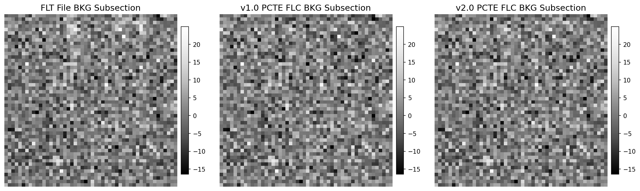
11.3 Display 50x50 Pixel Background Subsection#

One of the differences between the v1.0 and v2.0 CTE correction is the background level. Here, we show a square 50x50 pixel
subsection that is mostly featureless, i.e. no known sources or cosmic ray hits. The v2.0 correction significantly reduces noise
amplification and improves the resulting background. To aid in the visual inspection of the background subsection, an animated
GIF is included in the notebook that blinks between the v1.0 and v2.0 FLC files.

# Generate subplots
fig, [ax1, ax2, ax3] = plt.subplots(1, 3, figsize=(15, 10), dpi=150)

# Generate background subsections
flt_bkg = fltsci[2070:2120, 2180:2230]
v1_bkg = v1sci[2070:2120, 2180:2230]
v2_bkg = v2sci[2070:2120, 2180:2230]

# Calculate min and max values for image scaling 
z = ZScaleInterval()
z1, z2 = z.get_limits(v1_bkg)

# Display background subsection
im1 = ax1.imshow(flt_bkg, origin='lower', cmap='Greys_r', vmin=z1, vmax=z2)
im2 = ax2.imshow(v1_bkg, origin='lower', cmap='Greys_r', vmin=z1, vmax=z2)
im3 = ax3.imshow(v2_bkg, origin='lower', cmap='Greys_r', vmin=z1, vmax=z2)

# Formatting
fig.colorbar(im1, ax=ax1, shrink=0.35, pad=0.02)
fig.colorbar(im2, ax=ax2, shrink=0.35, pad=0.02)
fig.colorbar(im3, ax=ax3, shrink=0.35, pad=0.02)
ax1.set_title('FLT File BKG Subsection', size=14)
ax2.set_title('v1.0 PCTE FLC BKG Subsection', size=14)
ax3.set_title('v2.0 PCTE FLC BKG Subsection', size=14)
ax1.axis('off'), ax2.axis('off'), ax3.axis('off')
fig.tight_layout()

../../../_images/356230ae0c8fd5e3ea8ef99005598a1264f05d40405ab96eb09ebee321ab6a65.png

Animated GIF of the v1.0 and v2.0 FLC image subsections:

An animated gif blinking between a subsection of background sky using the v1.0 and V2.0 pixel-based CTE corrections. The v2.0 background appears smoother with less noise and pixel variations.

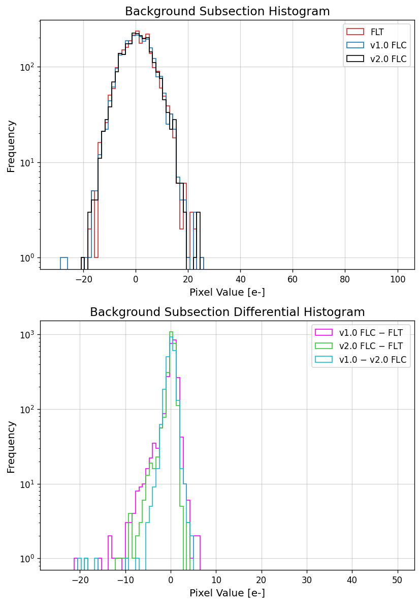
11.3.1 Pixel Distribution of Background Subsections#

To gain a more quantitative picture of how the background pixels are changing between the different file versions, we plot
the distribution of pixel values from the 50x50 pixel subsection above. The increased noise level in the v1.0 correction is
apparent in the blue histogram below. In addition, we have also computed the difference between the file types and have
plotted them as histograms. These two plots illustrates how the background in the v2.0 CTE corrected image is less noisy
and more in-line with the values seen in the FLT image.

# Generate subplots
fig, [ax1, ax2] = plt.subplots(2, 1, figsize=(7, 10), dpi=120)

# Plot background subsection histograms
ax1.hist(flt_bkg.ravel(), bins=100, range=(-30, 100), histtype='step', color='C3', label='FLT')
ax1.hist(v1_bkg.ravel(), bins=100, range=(-30, 100), histtype='step', color='C0', label='v1.0 FLC')
ax1.hist(v2_bkg.ravel(), bins=100, range=(-30, 100), histtype='step', color='k', label='v2.0 FLC')

# Plot background subsection differential histograms
ax2.hist((v1_bkg-flt_bkg).ravel(), bins=100, range=(-25, 50), histtype='step', color='magenta', label='v1.0 FLC $-$ FLT')
ax2.hist((v2_bkg-flt_bkg).ravel(), bins=100, range=(-25, 50), histtype='step', color='limegreen', label='v2.0 FLC $-$ FLT')
ax2.hist((v1_bkg-v2_bkg).ravel(), bins=100, range=(-25, 50), histtype='step', color='C9', label='v1.0 $-$ v2.0 FLC')

# Formatting
ax1.set_title('Background Subsection Histogram', size=14)
ax2.set_title('Background Subsection Differential Histogram', size=14)
ax1.set_xlabel('Pixel Value [e-]', size=12)
ax1.set_ylabel('Frequency', size=12)
ax2.set_xlabel('Pixel Value [e-]', size=12)
ax2.set_ylabel('Frequency', size=12)
ax1.grid(alpha=0.5), ax2.grid(alpha=0.5)
ax1.legend(), ax2.legend()
ax1.set_yscale('log')
ax2.set_yscale('log')
fig.tight_layout()

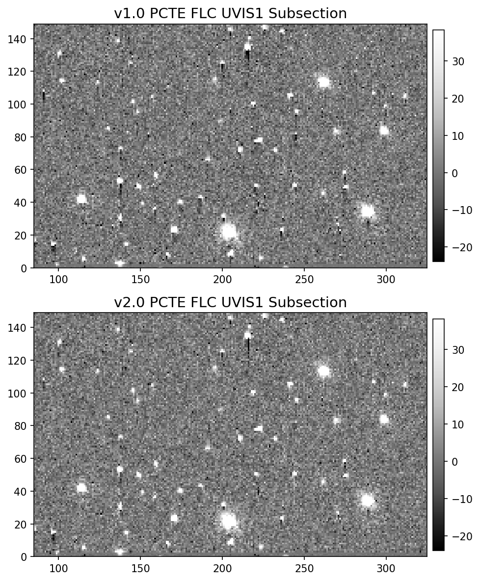
../../../_images/6e42ae78daaa5ebbc73c90ca0deb2da02e5fdae929e9aef3d6e5111787eb0405.png

11.4 Display Image Subsection#

Another difference between the v1.0 and v2.0 pixel-based CTE model is the amount of correction applied to fainter sources.
In order to reduce noise amplification, the fluxes of faint sources only receive a limited amount of correction in the v2.0 version.
We again provide an animated GIF of the two subsections to aid with the visual comparison.

# Generate subplots
fig, [ax1, ax2] = plt.subplots(2, 1, figsize=(8, 8), dpi=150)

# Calculate min and max values for image scaling 
z = ZScaleInterval()
z1, z2 = z.get_limits(v1_uvis1)

# Display subsection
im1 = ax1.imshow(v1_uvis1, origin='lower', cmap='Greys_r', vmin=z1, vmax=z2)
im2 = ax2.imshow(v2_uvis1, origin='lower', cmap='Greys_r', vmin=z1, vmax=z2)

# Formatting
ax1.set_xlim(85, 325), ax2.set_xlim(85, 325)
ax1.set_ylim(0, 149), ax2.set_ylim(0, 149)
fig.colorbar(im1, ax=ax1, shrink=0.95, pad=0.01)
fig.colorbar(im2, ax=ax2, shrink=0.95, pad=0.01)
ax1.set_title('v1.0 PCTE FLC UVIS1 Subsection', size=14)
ax2.set_title('v2.0 PCTE FLC UVIS1 Subsection', size=14)
fig.tight_layout()

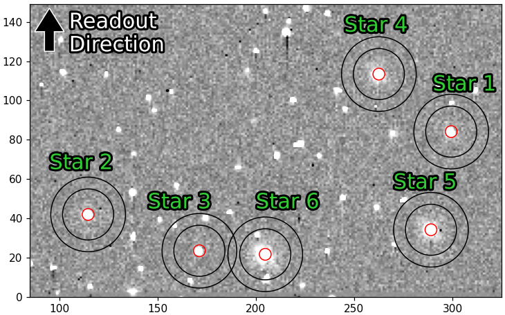
../../../_images/89e508e3da9550aa49ffb534964a0f35194dee1eba680edf3f54de605d17e308.png

Animated GIF of the v1.0 and v2.0 FLC image subsections:

11.5 Aperture Photometry#

To show the quantitative difference in the observed flux of sources between the v1.0 and v2.0 pixel-based CTE correction,
we perform aperture photometry on six stars of varying brightness within the image subsection above. Here, we display the
image subsection again with the apertures, annuli, and star labels overplotted. This subsection includes the first ~150 rows
of UVIS 1, which means all of these stars suffer the most CTE flux loss as they transfer 1900+ rows to the readout amplifier.

First, we approximate the center x and y positions of the stars in the 4Kx4K science arrays, and create the apertures and
annuli using photutils.

Then, we use photutils to measure the signal in each area and subtract the background values in the annuli from the
aperture sum values. We define a function named get_flux() to do this for us.

def get_flux(data, aperture, annulus_aperture):
    """
    Function to calculate background subtracted aperture sum 
    
    Parameters:
    -----------
    data : float array
        The 2d array of science pixels being measured
    aperture : photutils obj
        A photutils aperture object with defined position and radius
    annulus_aperture : photutils obj
        A photutils circular annulus aperture object with defined position and radii
        
    Return:
    -------
    flux : float
        The measured background subtracted aperture sum 
    """
    
    # Generate photutils.aperture_photometry table object
    phot = aperture_photometry(data, aperture)
    
    # Measure background around sources. aperture_stats_tbl() comes from background_median.py
    bkg_phot = aperture_stats_tbl(data, annulus_aperture, method='exact', sigma_clip=True)
    
    # Calculate background subtracted aperture sum
    flux = phot['aperture_sum'] - bkg_phot['aperture_median'] * aperture.area
    
    return flux


# Approximate x,y pixel locations of each star in the 4Kx4K array
positions = [(299.4, 2135.6),
             (114.7, 2093.4),
             (171.3, 2074.9),
             (262.6, 2164.9),
             (289.1, 2085.6),
             (204.8, 2073.1)]

# Photutils cirular aperture object with small radius
aperture = CircularAperture(positions, r=3)

# Photutils circular annulus aperture object 
annulus_aperture = CircularAnnulus(positions, r_in=13, r_out=19)

# Call function to calculate flux of stars
# THE RUNTIME WARNING MAY BE IGNORED
fltflux = get_flux(fltsci, aperture, annulus_aperture)
v1flux = get_flux(v1sci, aperture, annulus_aperture)
v2flux = get_flux(v2sci, aperture, annulus_aperture)

/home/runner/work/hst_notebooks/hst_notebooks/notebooks/WFC3/calwf3_v1.0_cte/example/background_median.py:88: RuntimeWarning: invalid value encountered in divide
  values = cutout * mask.data / mask.data
/home/runner/work/hst_notebooks/hst_notebooks/notebooks/WFC3/calwf3_v1.0_cte/example/background_median.py:88: RuntimeWarning: invalid value encountered in divide
  values = cutout * mask.data / mask.data
/home/runner/work/hst_notebooks/hst_notebooks/notebooks/WFC3/calwf3_v1.0_cte/example/background_median.py:88: RuntimeWarning: invalid value encountered in divide
  values = cutout * mask.data / mask.data

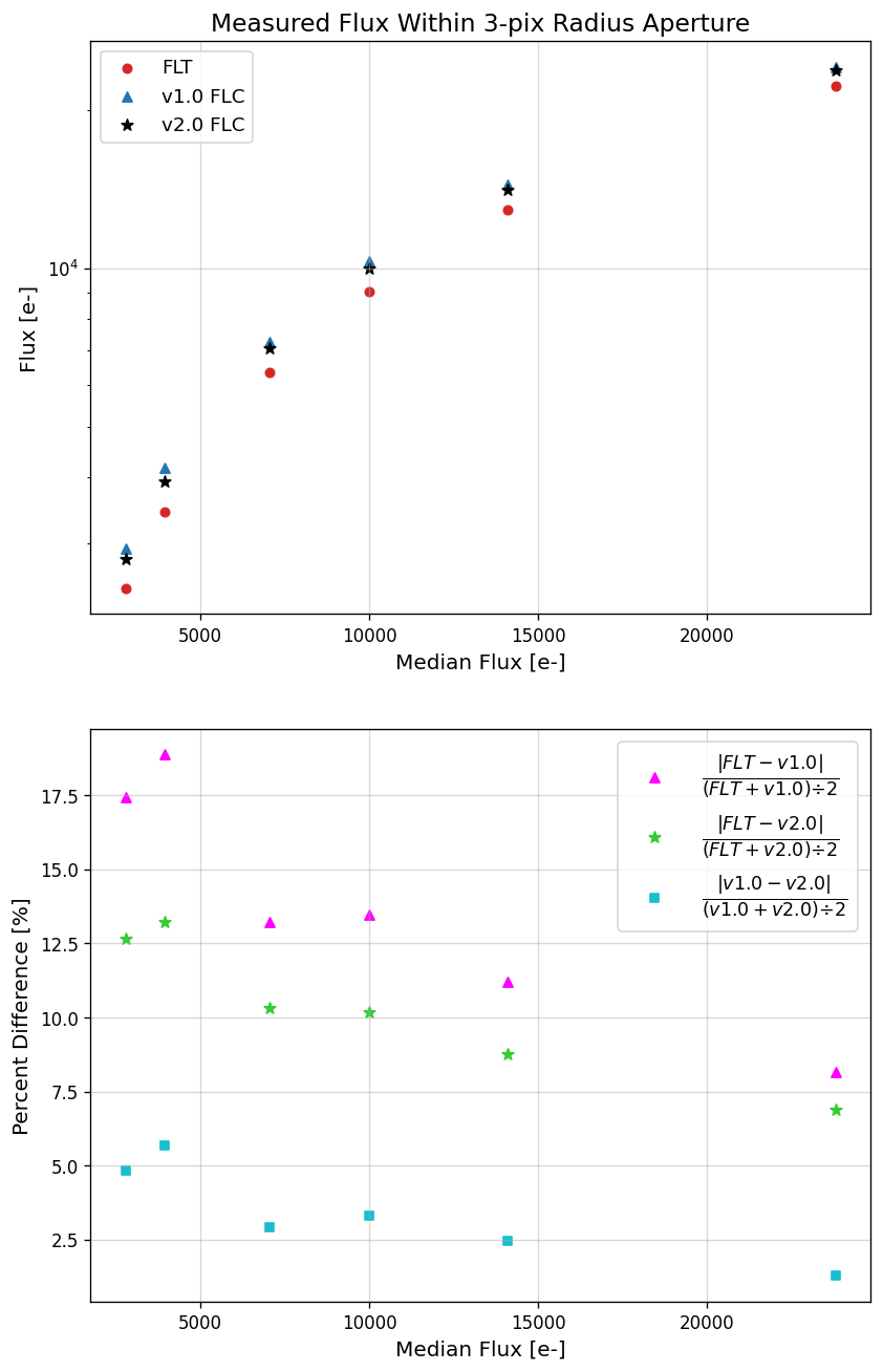
You can ignore the RuntimeWarning: invalid value encountered in true_divide message.

Finally, we plot our results.

The first plot below shows the measured flux of the six stars in each of the different calibrated products. Stars 1-6 are organized
by increasing flux, with Star 1 being the faintest and Star 6 being the brightest. The x-axis values correspond to the median flux
value measured in each of the three different files (FLT, v1.0, and v2.0) per star. The y-axis values show the individual flux values
for each star where the different colors and symbols represent the three file types. For example, the individual flux values (y-axis)
of Star 1 for the FLT, v1.0, and v2.0 files are ~2467, 3056, and 2799 e- respectively. The median of the three values is ~2799 e-,
which is the value plotted on the x-axis. The second plot illustrates the percent differences between the three different
flux values per star, and uses the same x-axis values as the first plot.

The FLT files have no CTE correction applied and thus have the lowest measured flux for each star due to the CTE flux loss.
Stars 1-4 have noticably different flux values between the v1.0 and v2.0 CTE corrections. In v1.0, the CTE algorithm is actually
over-correcting these fainter sources resulting in higher aperture photometry measurements. The flux values for stars 1-4 range
from ~3000 - 10000 e- within a 3-pixel radius aperture. The flux values between the v1.0 and v2.0 CTE corrections for stars
1-4 have percent differences of ~9 - 4%. Sources with more than ~10000 e- within a 3-pixel aperture (stars 5 & 6) have more
compareable flux values between the v1.0 and v2.0 CTE corrections, and have percent differences less than 2%.

# Generate subplots
fig, [ax1, ax2] = plt.subplots(2, 1, figsize=(8, 13), dpi=120)
ax1.grid(alpha=0.5), ax2.grid(alpha=0.5)

# Find median flux values between products
medflux = np.median([fltflux, v1flux, v2flux], axis=0)

# Scatter plot of measured flux
ax1.scatter(medflux, fltflux, 25, marker='o', c='C3', label='FLT')
ax1.scatter(medflux, v1flux, 30, marker='^', c='C0', label='v1.0 FLC')
ax1.scatter(medflux, v2flux, 45, marker='*', c='k', label='v2.0 FLC')

# Scatter plot of percentage difference
ax2.scatter(medflux, abs((fltflux-v1flux))/((fltflux+v1flux)/2)*100, 30,
            marker='^', c='magenta', label=r'$\frac{|FLT - v1.0|}{(FLT + v1.0) ÷ 2}$')
ax2.scatter(medflux, abs((fltflux-v2flux))/((fltflux+v2flux)/2)*100, 45,
            marker='*', c='limegreen', label=r'$\frac{|FLT - v2.0|}{(FLT + v2.0) ÷ 2}$')
ax2.scatter(medflux, abs((v1flux-v2flux))/((v1flux+v2flux)/2)*100, 25,
            marker='s', c='C9', label=r'$\frac{|v1.0 - v2.0|}{(v1.0 + v2.0) ÷ 2}$')

# Formatting 
ax1.set_title('Measured Flux Within 3-pix Radius Aperture', size=14)
ax1.set_xlabel('Median Flux [e-]', size=12)
ax1.set_ylabel('Flux [e-]', size=12)
ax2.set_xlabel('Median Flux [e-]', size=12)
ax2.set_ylabel('Percent Difference [%]', size=12)
ax1.legend(prop={'size': 11}), ax2.legend(prop={'size': 15})
ax1.set_yscale('log')

../../../_images/d94c5a5e851de5be85a7e68a094cde6ac8a1cf949a4846935c7afab6398971a6.png

12. Conclusions#

Thank you for walking through this notebook. You now have everything you need to process your own files with the v1.0 CTE
correction within calwf3. Since completing this notebook you should be more familiar with:

Applying the v1.0 pixel-based CTE correction to 2009-2021 UVIS data.
Which header keywords of the raw fits file to edit in order to use the v1.0 correction.
How to find and download the appropriate PCTETAB and DRKCFILE reference files.
Verifying your version of calwf3 and calibrating a raw file with the v1.0 CTE correction.
Investigating the differences between v1.0 and v2.0 CTE corrected files.

Congratulations, you have completed the notebook!#

Additional Resources#

Below are some additional resources that may be helpful. Please feel free to contact the WFC3 Helpdesk for any questions.

About this Notebook#

Author: Benjamin Kuhn; WFC3 Instrument Team
Created: February 22, 2022
Last updated on: November 15, 2023

Citations#

If you use astropy, astroquery, numpy, matplotlib, photutils, or scipy for published research, please cite the authors.
Follow these links for more information about citing the libraries below:

Top of Page

Processing WFC3/UVIS Data with calwf3 Using the v1.0 CTE-Correction

Contents

Processing WFC3/UVIS Data with calwf3 Using the v1.0 CTE-Correction#

Learning Goals#

Table of Contents#

Introduction#

1. Imports#

2. Verify archived_drkcfiles.txt is in CWD#

3. Check that calwf3 Version is v3.5.2#

4. Query MAST and Download a WFC3 raw.fits Image#

5. Set CRDS Environment Variable and Download Reference Files#

5.1 Run crds bestrefs#

5.2 Inspect Image Header#

6. Find the Correct v1.0 DRKCFILE#

6.1 Download the Correct DRKCFILE from CRDS#

6.2 Modify the Image Header Keyword, DRKCFILE#

7. Download the v1.0 PCTETAB#

7.1 Modify the Image Header Keyword, PCTETAB#

8. Re-Inspect Image Header#

9. Run calwf3#

10. Inspect FLC Image Header#

11. Investigate v1.0 and v2.0 Differences#

11.1 Download the v2.0 FLC File#

11.2 Open Files#

11.3 Display 50x50 Pixel Background Subsection#

11.3.1 Pixel Distribution of Background Subsections#

11.4 Display Image Subsection#

11.5 Aperture Photometry#

12. Conclusions#

Congratulations, you have completed the notebook!#

Additional Resources#

About this Notebook#

Citations#

Processing WFC3/UVIS Data with `calwf3` Using the v1.0 CTE-Correction#

2. Verify `archived_drkcfiles.txt` is in CWD#

3. Check that `calwf3` Version is `v3.5.2`#

4. Query MAST and Download a WFC3 `raw.fits` Image#

5.1 Run `crds bestrefs`#

6. Find the Correct v1.0 `DRKCFILE`#

6.1 Download the Correct `DRKCFILE` from CRDS#

6.2 Modify the Image Header Keyword, `DRKCFILE`#

7. Download the v1.0 `PCTETAB`#

7.1 Modify the Image Header Keyword, `PCTETAB`#

9. Run `calwf3`#