Viewing STIS Data

Learning Goals

By the end of this tutorial, you will go through:

• 0.Introduction

  • 0.1 Import necessary packages

• 1. Downloading STIS data from MAST using astroquery

• 2. Reading in the data

  • 2.1 Investigating the data - Basics

  • 2.2 Reading the table data

• 3. Plotting the spectrum

  • 3.1 Making a simple plot of the spectrum

• 4. Working with data quality flags

  • 4.1 Data quality frequencies histogram

  • 4.2 Removing “Serious Data Quality”

• 5. Visualizing STIS Image

  • 5.1 Exploring image file structure

  • 5.2 Showing the image

  • 5.3 Removing serious data quality pixels

• 6.Working with Time-Tag Data

  • 6.1 Investigating the _tag Data

  • 6.2 Converting Time_Tag into ACCUM image

• 7.Working with STIS Echelle data

  • 7.1 Showing Echelle Image

  • 7.2 Plotting Echelle Spectrum

0. Introduction

The Space Telescope Imaging Spectrograph (STIS) is a versatile imaging spectrograph installed on the Hubble Space Telescope (HST), covering a wide range of wavelengths from the near-infrared region into the ultraviolet.

This tutorial aims to prepare new users to begin analyzing STIS data by going through downloading data, reading and viewing spectra, and viewing STIS images.

There are three detectors on STIS: FUV-MAMA, NUV-MAMA, and CCD. While the detectors are designed for different scientific purposes and operate at a different wavelength, their data are organized in the same structure. Thus we are using FUV-MAMA data as an example in this notebook.

For a detailed overview of the STIS instrument, see the STIS Instrument Handbook.
For more information on STIS data analysis and operations, see the STIS Data Handbook.

Defining some terms:

• HST: Hubble Space Telescope

• STIS: Space Telescope Imaging Spectrograph on HST (https://www.stsci.edu/hst/instrumentation/stis)

• STIS/NUV-MAMA: Cs2Te Multi-Anode Microchannel Array (MAMA) detector for observing mainly in the near ultraviolet (NUV)

• STIS/FUV-MAMA: Solar-blind CsI Multi-Anode Microchannel Array (MAMA) detector for observing mainly in the far ultraviolet (FUV)

• CCD: Charge Coupled Device

• FITS: Flexible Image Transport System (https://fits.gsfc.nasa.gov/fits_primer.html)

• HDU: Header/Data Unit in a FITS file

0.1 Import necessary packages

We will import the following packages:

• astropy.io.fits for accessing FITS files

• astropy.table.Table for creating tidy tables of the data

• astroquery.mast.Observations for finding and downloading data from the MAST archive

• pathlib for managing system paths

• matplotlib.pyplot for plotting data

• IPython.display for formatting display

• numpy to handle array functions

• pandas to make basic tables and dataframes

• stistools for operations on STIS data

# Import for: Reading in fits file
from astropy.table import Table
from astropy.io import fits

# Import for: Downloading necessary files. (Not necessary if you choose to collect data from MAST)
from astroquery.mast import Observations

# Import for: Managing system variables and paths
from pathlib import Path

# Import for: Plotting and specifying plotting parameters
import matplotlib.pyplot as plt
import matplotlib
import matplotlib.cm as cm
from IPython.display import display

# Import for: Quick Calculation and Data Analysis
import numpy as np
import pandas as pd

# Import for operations on STIS Data
import stistools

The following tasks in the stistools package can be run with TEAL:
   basic2d      calstis     ocrreject     wavecal        x1d          x2d

/opt/hostedtoolcache/Python/3.11.9/x64/lib/python3.11/site-packages/stsci/tools/nmpfit.py:8: UserWarning: NMPFIT is deprecated - stsci.tools v 3.5 is the last version to contain it.
  warnings.warn("NMPFIT is deprecated - stsci.tools v 3.5 is the last version to contain it.")
/opt/hostedtoolcache/Python/3.11.9/x64/lib/python3.11/site-packages/stsci/tools/gfit.py:18: UserWarning: GFIT is deprecated - stsci.tools v 3.4.12 is the last version to contain it.Use astropy.modeling instead.
  warnings.warn("GFIT is deprecated - stsci.tools v 3.4.12 is the last version to contain it."

1. Downloading STIS data from MAST using astroquery

There are other ways to download data from MAST such as using CyberDuck. We are only showing how to use astroquery in this notebook

# make directory for downloading data
datadir = Path('./data')
datadir.mkdir(exist_ok=True)

# Search target object by obs_id
target = Observations.query_criteria(obs_id='ODJ102010')
# get a list of files assiciated with that target
FUV_list = Observations.get_product_list(target)
# Download only the SCIENCE fits files
downloads = Observations.download_products(
    FUV_list,
    productType='SCIENCE',
    extension='fits',
    download_dir=str(datadir))
downloads

Downloading URL https://mast.stsci.edu/api/v0.1/Download/file?uri=mast:HST/product/odj102010_raw.fits to data/mastDownload/HST/odj102010/odj102010_raw.fits ...

 [Done]

Downloading URL https://mast.stsci.edu/api/v0.1/Download/file?uri=mast:HST/product/odj102010_flt.fits to data/mastDownload/HST/odj102010/odj102010_flt.fits ...

 [Done]

Downloading URL https://mast.stsci.edu/api/v0.1/Download/file?uri=mast:HST/product/odj102010_x2d.fits to data/mastDownload/HST/odj102010/odj102010_x2d.fits ...

 [Done]

Downloading URL https://mast.stsci.edu/api/v0.1/Download/file?uri=mast:HST/product/odj102010_x1d.fits to data/mastDownload/HST/odj102010/odj102010_x1d.fits ...

 [Done]

Downloading URL https://mast.stsci.edu/api/v0.1/Download/file?uri=mast:HST/product/hasp/hst_15168_stis_-alf-cep_g140m_odj1_cspec.fits to data/mastDownload/HST/hst_hasp_15168_stis_-alf-cep_odj1/hst_15168_stis_-alf-cep_g140m_odj1_cspec.fits ...

 [Done]

Downloading URL https://mast.stsci.edu/api/v0.1/Download/file?uri=mast:HST/product/hasp/hst_15168_stis_-alf-cep_g140m_odj102_cspec.fits to data/mastDownload/HST/hst_hasp_15168_stis_-alf-cep_odj1/hst_15168_stis_-alf-cep_g140m_odj102_cspec.fits ...

 [Done]

Table length=6

Local Path	Status	Message	URL
str103	str8	object	object
data/mastDownload/HST/odj102010/odj102010_raw.fits	COMPLETE	None	None
data/mastDownload/HST/odj102010/odj102010_flt.fits	COMPLETE	None	None
data/mastDownload/HST/odj102010/odj102010_x2d.fits	COMPLETE	None	None
data/mastDownload/HST/odj102010/odj102010_x1d.fits	COMPLETE	None	None
data/mastDownload/HST/hst_hasp_15168_stis_-alf-cep_odj1/hst_15168_stis_-alf-cep_g140m_odj1_cspec.fits	COMPLETE	None	None
data/mastDownload/HST/hst_hasp_15168_stis_-alf-cep_odj1/hst_15168_stis_-alf-cep_g140m_odj102_cspec.fits	COMPLETE	None	None

2. Reading in the data

2.1 Investigating the data - Basics

Before doing any operations on the data, we want to first explore the basics and data file structures.

The 1D-extracted, background subtracted, flux and wavelength calibrated spectra data are stored in a FITS file with suffix _x1d (note that for the CCD it is _sx1). While we are using the _x1d FITS file as an example of investigating STIS data, the following methods for reading in data and viewing a spectra or other fields can be applied to the other STIS data, either calibrated or uncalibrated. For more information on STIS file naming conventions, see Types of STIS Files in the STIS Data Handbook.

Open the x1d fits file and explore its info and header:

# get information about the fits file
x1d_file = Path('./data/mastDownload/HST/odj102010/odj102010_x1d.fits')
fits.info(x1d_file)

Filename: data/mastDownload/HST/odj102010/odj102010_x1d.fits
No.    Name      Ver    Type      Cards   Dimensions   Format
  0  PRIMARY       1 PrimaryHDU     274   ()      
  1  SCI           1 BinTableHDU    157   1R x 19C   [1I, 1I, 1024D, 1024E, 1024E, 1024E, 1024E, 1024E, 1024E, 1024I, 1E, 1E, 1I, 1E, 1E, 1E, 1E, 1024E, 1E]   

The primary header that stores keyword information describing the global properties of all of the exposures in the file

# get header of the fits file
x1d_header_0 = fits.getheader(x1d_file, ext=0)

for key in ["INSTRUME", "DETECTOR", "OBSMODE", "OPT_ELEM", "CENWAVE", "PROPAPER", "TARGNAME"]:
    print(f"{key}:\t{x1d_header_0[key]}")   

INSTRUME:	STIS
DETECTOR:	FUV-MAMA
OBSMODE:	ACCUM
OPT_ELEM:	G140M
CENWAVE:	1540
PROPAPER:	52X0.2
TARGNAME:	-ALF-CEP

You can change the keys to check for other fields and metadata, or directly print the x1d_header_0 to get all header information.

Some other metadata, such as exposure data and time, are stored in the first extension.

x1d_header_1 = fits.getheader(x1d_file, ext=1)

date = x1d_header_1["DATE-OBS"]
time = x1d_header_1["Time-OBS"]
exptime = x1d_header_1["EXPTIME"]

print(f"The data were taken on {date}, starting at {time}, with the exposure time of {exptime} seconds")

The data were taken on 2018-01-14, starting at 08:31:01, with the exposure time of 900.0 seconds

2.2 Reading table data

The main science data is stored in the first extension of the x1d FITS file. We first read in the data as an astropy Table.

# Get data
x1d_data = Table.read(x1d_file, hdu=1)
# Display a representation of the data:
x1d_data

WARNING: UnitsWarning: 'Angstroms' did not parse as fits unit: At col 0, Unit 'Angstroms' not supported by the FITS standard. Did you mean Angstrom or angstrom? If this is meant to be a custom unit, define it with 'u.def_unit'. To have it recognized inside a file reader or other code, enable it with 'u.add_enabled_units'. For details, see https://docs.astropy.org/en/latest/units/combining_and_defining.html [astropy.units.core]
WARNING: UnitsWarning: 'Counts/s' did not parse as fits unit: At col 0, Unit 'Counts' not supported by the FITS standard. Did you mean count? If this is meant to be a custom unit, define it with 'u.def_unit'. To have it recognized inside a file reader or other code, enable it with 'u.add_enabled_units'. For details, see https://docs.astropy.org/en/latest/units/combining_and_defining.html [astropy.units.core]
WARNING: UnitsWarning: 'erg/s/cm**2/Angstrom' contains multiple slashes, which is discouraged by the FITS standard [astropy.units.format.generic]

Table length=1

SPORDER	NELEM	WAVELENGTH	GROSS	BACKGROUND	NET	FLUX	ERROR	NET_ERROR	DQ	A2CENTER	EXTRSIZE	MAXSRCH	BK1SIZE	BK2SIZE	BK1OFFST	BK2OFFST	EXTRLOCY	OFFSET
		Angstroms	Counts/s	Counts/s	Counts/s	erg / (Angstrom s cm2)	erg / (Angstrom s cm2)	Counts/s		pix	pix	pix	pix	pix	pix	pix	pix	pix
int16	int16	float64[1024]	float32[1024]	float32[1024]	float32[1024]	float32[1024]	float32[1024]	float32[1024]	int16[1024]	float32	float32	int16	float32	float32	float32	float32	float32[1024]	float32
1	1024	1513.611692349868 .. 1567.668670092399	1.423279 .. 0.04860059	0.0008550065 .. -6.92308e-05	1.422424 .. 0.04866982	1.96904e-12 .. 9.89624e-14	5.507516e-14 .. 1.495948e-14	0.03978601 .. 0.007357089	2564 .. 2564	389.5777	11	1024	5	5	-300	300	382.2857 .. 397.2364	351.8867

# We can also get the columns of this table:
columns = x1d_data.colnames
columns

['SPORDER',
 'NELEM',
 'WAVELENGTH',
 'GROSS',
 'BACKGROUND',
 'NET',
 'FLUX',
 'ERROR',
 'NET_ERROR',
 'DQ',
 'A2CENTER',
 'EXTRSIZE',
 'MAXSRCH',
 'BK1SIZE',
 'BK2SIZE',
 'BK1OFFST',
 'BK2OFFST',
 'EXTRLOCY',
 'OFFSET']

Another common way of reading in FITS data from an HDU list as “FITS_rec”:

with fits.open(x1d_file) as hdulist:
    fuv_x1d_data = hdulist[1].data
    
type(fuv_x1d_data)

astropy.io.fits.fitsrec.FITS_rec

3. Plotting the spectrum

3.1 Making a simple plot of the spectrum

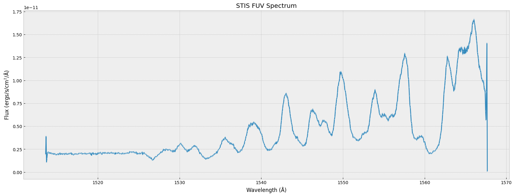
The actual data of each column are stored in arrays within each row with equal lengths. We collect the spectrum data and plot them with corresponding error bars.

# From the astropy table, we first get all the data we need: wavelength, flux, and error
# notice that for astropy table, the column name is case sensitive
# First-order data have data in only the 0th row, so we extract this sparse dimension.
wl, flux, err = x1d_data[0]['WAVELENGTH', 'FLUX', 'ERROR']

# Make a plot of the data, use this cell to specify the format of the plot.
matplotlib.rcParams['figure.figsize'] = [20, 7]
plt.style.use('bmh')

plt.plot(wl, flux,  # the x-data & y-data
         marker='.', markersize=2, markerfacecolor='w', markeredgewidth=0) # specifies the data points style
plt.fill_between(wl, flux - err, flux + err, alpha=0.5)  # shade regions by width of error array
plt.title('STIS FUV Spectrum')
plt.xlabel('Wavelength (Å)')
plt.ylabel('Flux (ergs/s/cm$^2$/Å)')

Text(0, 0.5, 'Flux (ergs/s/cm$^2$/Å)')

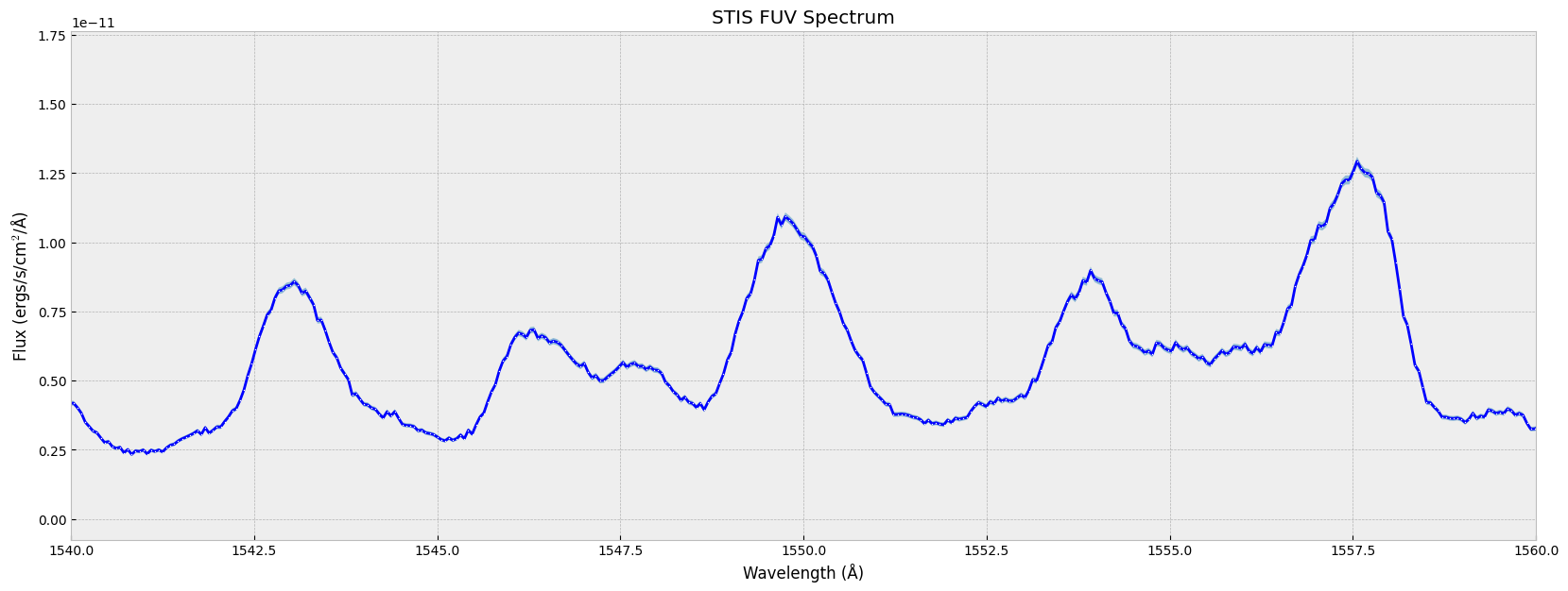
You can zoom in to a specific wavelength range

# plot the spectrum between 1540 and 1560 Å:
plt.plot(wl, flux,  # the x-data & y-data
         marker='.', markersize=2, markerfacecolor='w', markeredgewidth=0,  # specifies the data point style
         color='blue')  # specifies the format of lines
plt.fill_between(wl, flux - err, flux + err, alpha=0.5)  # shade regions by width of error array
plt.title('STIS FUV Spectrum')
plt.xlabel('Wavelength (Å)')
plt.ylabel("Flux (ergs/s/cm$^2$/Å)")
plt.xlim(1540, 1560)

(1540.0, 1560.0)

You can also plot the error bar together with the spectrum. For more errorbar styling options, see matplotlib.pyplot.errorbar

plt.errorbar(wl, flux, err,  # the x-data, y-data, and y-axis error
             marker='.', markersize=2, markerfacecolor='w', markeredgewidth=0, color='blue',  # specifies the data points style
             ecolor='dodgerblue', capsize=0.1)  # specifies the format of lines and error bar
plt.title('STIS FUV Spectrum')
plt.xlabel('Wavelength (Å)')
plt.ylabel('Flux (ergs/s/cm$^2$/Å)')
plt.xlim(1540, 1560)

(1540.0, 1560.0)

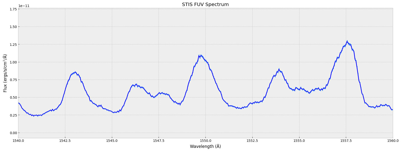
For more information on formatting the plots using matplotlib, see matplotlib.pyplot.plot, matplotlib.pyplot.errorbar.

4.Working with data quality flags

Data quality flags are assigned to each pixel in the data quality extension. Each flag has a true (set) or false (unset) state. Flagged conditions are set as specific bits in a 16-bit integer word. For a single pixel, this allows for up to 15 data quality conditions to be flagged simultaneously, using the bitwise logical OR operation. Note that the data quality flags cannot be interpreted simply as integers but may be converted to base-2 and interpreted as flags. These flags are set and used during the course of calibration, and may likewise be interpreted and used by downstream analysis applications.

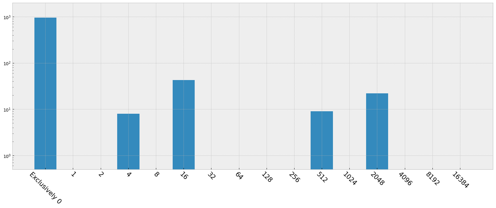
4.1 Data quality frequencies histogram

Make a histogram according to the data quality flags, and label the bins by what each data quality values actually means. More info: https://hst-docs.stsci.edu/stisdhb/chapter-2-stis-data-structure/2-5-error-and-data-quality-array

# First get the possible data quality flag values to bitwise-and with the data quality flag:
dq_flags = ['Exclusively 0'] + list(1 << np.arange(0, 15))

dq_bits = {}
# In the Table representation, the data quality flag is a masked array that "hides" the pixels
# with no data quality issue. We fill those "good points" with 0 here when counting:
dq_bits[0] = np.count_nonzero(x1d_data[0]['DQ'].filled(0) == 0)  # exclusively 0

# Loop over non-zero flag values and count each:
for dq_flag in dq_flags[1:]:
    dq_bits[dq_flag] = np.count_nonzero((x1d_data[0]['DQ'] & dq_flag))

dq_bits

{0: 960,
 1: 0,
 2: 0,
 4: 8,
 8: 0,
 16: 43,
 32: 0,
 64: 0,
 128: 0,
 256: 0,
 512: 9,
 1024: 0,
 2048: 22,
 4096: 0,
 8192: 0,
 16384: 0}

# Assign the meaning of each data quality and make a histogram
meanings = {
    0:  "No Anomalies",
    1:  "Error in the Reed Solomon decoding",
    2:  "Lost data replaced by fill values",
    3:  "Bad detector pixel (e.g., bad column or row, mixed science and bias for overscan, or beyond aperture)",
    4:  "Data masked by occulting bar",
    5:  "Pixel having dark rate > 5 σ times the median dark level",
    6:  "Large blemish, depth > 40% of the normalized p-flat (repeller wire)",
    7:  "Vignetted pixel",
    8:  "Pixel in the overscan region",
    9:  "Saturated pixel, count rate at 90% of max possible—local non-linearity turns over and is multi-valued; "
        "pixels within 10% of turnover and all pixels within 4 pixels of that pixel are flagged.",
    10: "Bad pixel in reference file",
    11: "Small blemish, depth between 40% and 70% of the normalized flat. Applies to MAMA and CCD p-flats",
    12: ">30% of background pixels rejected by sigma-clip, or flagged, during 1-D spectral extraction",
    13: "Extracted flux affected by bad input data",
    14: "Data rejected in input pixel during image combination for cosmic ray rejection",
    15: "Extracted flux not CTI corrected because gross counts are ≤ 0"}

plt.bar(meanings.keys(), height=dq_bits.values(), tick_label=dq_flags)
plt.gca().set_xticklabels(dq_flags, rotation=-45, fontsize=15)
plt.yscale('log')
plt.ylim(0.5, 2000)
plt.show()

bits = [f'{0:015b}'] + [f'{1 << x:015b}' for x in range(0, 15)]

dq_table = pd.DataFrame({
    "Flag Value": dq_flags,
    "Bit Setting": bits,
    "Quality Condition Indicated": meanings.values()})
dq_table.set_index('Flag Value', drop=True, inplace=True)

pd.set_option('display.max_colwidth', None)
display(dq_table)

	Bit Setting	Quality Condition Indicated
Flag Value
Exclusively 0	000000000000000	No Anomalies
1	000000000000001	Error in the Reed Solomon decoding
2	000000000000010	Lost data replaced by fill values
4	000000000000100	Bad detector pixel (e.g., bad column or row, mixed science and bias for overscan, or beyond aperture)
8	000000000001000	Data masked by occulting bar
16	000000000010000	Pixel having dark rate > 5 σ times the median dark level
32	000000000100000	Large blemish, depth > 40% of the normalized p-flat (repeller wire)
64	000000001000000	Vignetted pixel
128	000000010000000	Pixel in the overscan region
256	000000100000000	Saturated pixel, count rate at 90% of max possible—local non-linearity turns over and is multi-valued; pixels within 10% of turnover and all pixels within 4 pixels of that pixel are flagged.
512	000001000000000	Bad pixel in reference file
1024	000010000000000	Small blemish, depth between 40% and 70% of the normalized flat. Applies to MAMA and CCD p-flats
2048	000100000000000	>30% of background pixels rejected by sigma-clip, or flagged, during 1-D spectral extraction
4096	001000000000000	Extracted flux affected by bad input data
8192	010000000000000	Data rejected in input pixel during image combination for cosmic ray rejection
16384	100000000000000	Extracted flux not CTI corrected because gross counts are ≤ 0

4.2 Removing “Serious Data Quality Flags”

Through the calibaration pipeline, some data qualities are marked “serious”. The value of serious data qualities are marked through “SDQFLAGS”. We can decompose that value according to the bits in order to see the specific data quality flags that are marked serious.

sdqFlags_fuv = fits.getval(x1d_file, ext=1, keyword="SDQFLAGS")
print(f'The SDQFLAGS is {sdqFlags_fuv}, which is in binary {sdqFlags_fuv:015b},')
print('Therefore the following data qualities are marked "serious":')
for i in range(15):
    if 2**i & sdqFlags_fuv:
        print(f'\t{i+1:2.0f}: ' + meanings[i+1])

The SDQFLAGS is 31743, which is in binary 111101111111111,
Therefore the following data qualities are marked "serious":
	 1: Error in the Reed Solomon decoding
	 2: Lost data replaced by fill values
	 3: Bad detector pixel (e.g., bad column or row, mixed science and bias for overscan, or beyond aperture)
	 4: Data masked by occulting bar
	 5: Pixel having dark rate > 5 σ times the median dark level
	 6: Large blemish, depth > 40% of the normalized p-flat (repeller wire)
	 7: Vignetted pixel
	 8: Pixel in the overscan region
	 9: Saturated pixel, count rate at 90% of max possible—local non-linearity turns over and is multi-valued; pixels within 10% of turnover and all pixels within 4 pixels of that pixel are flagged.
	10: Bad pixel in reference file
	12: >30% of background pixels rejected by sigma-clip, or flagged, during 1-D spectral extraction
	13: Extracted flux affected by bad input data
	14: Data rejected in input pixel during image combination for cosmic ray rejection
	15: Extracted flux not CTI corrected because gross counts are ≤ 0

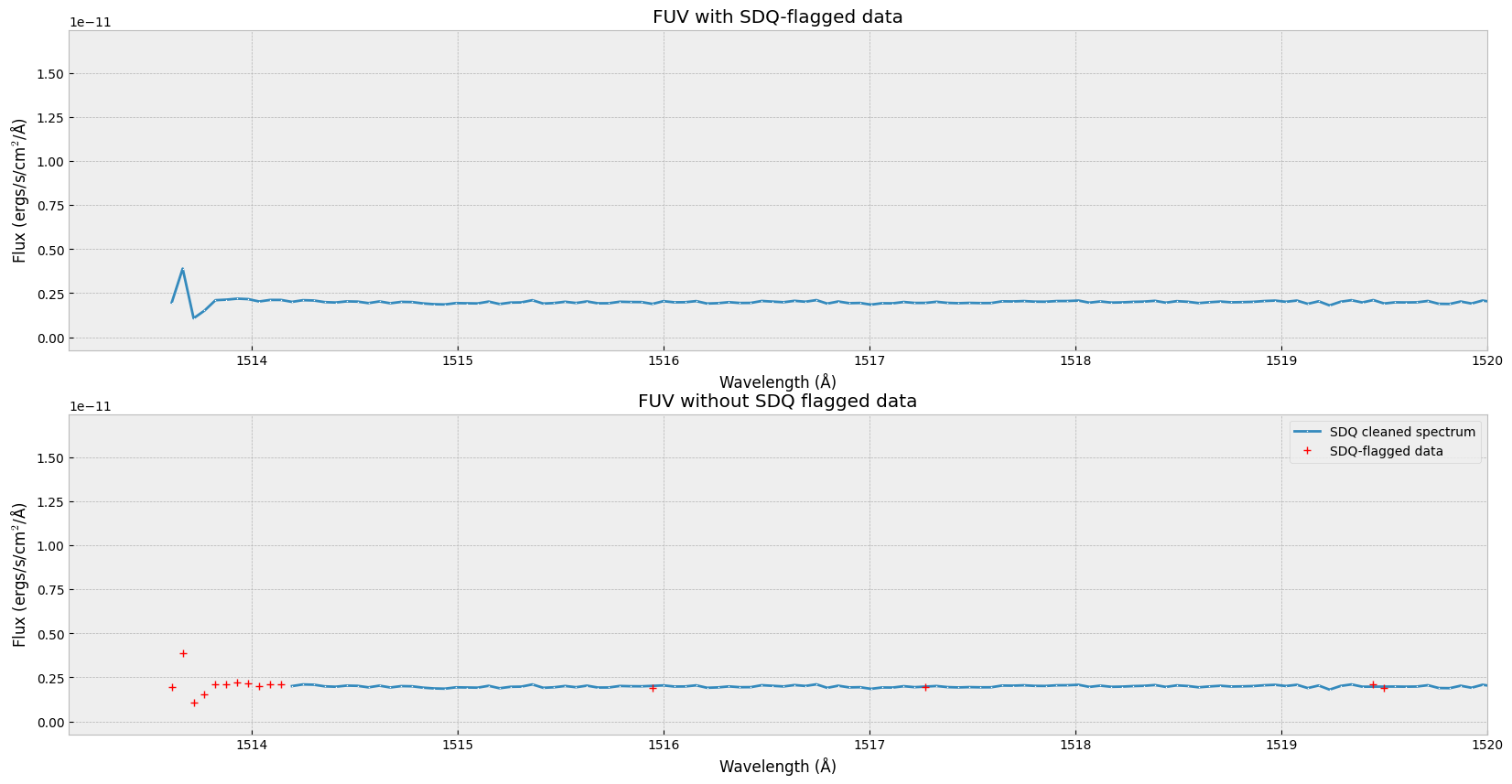
We can now remove the data points with SDQ flags. In the plots below, the first one is the same as the spectrum in which we do not handle the SDQ flags. The second one is the spectrum with SDQ flagged data removed, and the SDQ flagged data points are marked with red ‘+’.

fig, axes = plt.subplots(2, 1)
fig.set_size_inches(20, 10)
plt.style.use('bmh')

# First zoom in to the region where SDQ got removed
wl, flux, err, dq = x1d_data[0]['WAVELENGTH', 'FLUX', 'ERROR', 'DQ']

# Filter the datapoints to where there are no serious DQ flags
mask_noSDQ = (dq & sdqFlags_fuv) == 0

# get the spectrum without SDQ using the mask we just created
wvln_noSDQ, flux_noSDQ, err_noSDQ = wl[mask_noSDQ], flux[mask_noSDQ], err[mask_noSDQ]
# inverse the _noSDQ mask to collect the data points with SDQ flags
wvln_SDQ, flux_SDQ = wl[~mask_noSDQ], flux[~mask_noSDQ]  # apply the bitwise-not of mask

# plot1: the spectrum with SDQ flagged data included
# plt.subplot(2,1,1)
axes[0].plot(wl, flux,  # the x-data, y-data
             marker='.', markersize=2, markerfacecolor='w', markeredgewidth=0)  # specifies the data points style

# plot2: plot the spectrum without SDQ flagged data, then mark the SDQ data points with +
# Plot the filtered datapoints
axes[1].plot(wvln_noSDQ, flux_noSDQ,  # the x-data, y-data
             marker='.', markersize=2, markerfacecolor='w', markeredgewidth=0, label="SDQ cleaned spectrum")
axes[1].plot(wvln_SDQ, flux_SDQ, 'r+', label='SDQ-flagged data')
axes[1].legend(loc='best')

# Format the figures:
axes[0].set_title('FUV with SDQ-flagged data')
axes[1].set_title('FUV without SDQ flagged data')
for ax in axes:
    ax.set_xlabel('Wavelength (Å)')
    ax.set_ylabel('Flux (ergs/s/cm$^2$/Å)')
    ax.set_xlim(wl.min() - 0.5, 1520)  # zoom in on left edge

5. Visualizing STIS Image

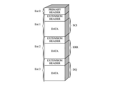
The STIS images are stored as two-dimensional arrays in FITS image extension files. For more information on STIS image files and extension, see STIS FITS Image Extension Files

5.1 Exploring image file structure

The rectified, wavelength and flux calibrated first order spectra or Geometrically corrected imaging data is stored in the fits file with the x2d extension (note that for the CCD the similar extension is sx2). Similar to what we did to the x1d file, we first open the fits file to explore its file structure.

# read in the x2d file and get its info
x2d_file = Path('./data/mastDownload/HST/odj102010/odj102010_x2d.fits')
fits.info(x2d_file)

Filename: data/mastDownload/HST/odj102010/odj102010_x2d.fits
No.    Name      Ver    Type      Cards   Dimensions   Format
  0  PRIMARY       1 PrimaryHDU     277   ()      
  1  SCI           1 ImageHDU       121   (1201, 1201)   float32   
  2  ERR           1 ImageHDU        61   (1201, 1201)   float32   
  3  DQ            1 ImageHDU        44   (1201, 1201)   int16   

• The first, of extension type SCI, stores the science count/flux values.

• The second, of extension type ERR, contains the statistical errors, which are propagated through the calibration process. It is unpopulated in raw data files.

• The third, of extension type DQ, stores the data quality values, which flag suspect pixels in the corresponding SCI data. It is unpopulated in raw data files.

Similarly, we can also get the header from this FITS file to see the scientific metadata.

# get header of the fits file
x2d_header = fits.getheader(x2d_file, ext=0)
x2d_header[:15]  # additional lines are not displayed here

SIMPLE  =                    T / file does conform to FITS standard             
BITPIX  =                   16 / number of bits per data pixel                  
NAXIS   =                    0 / number of data axes                            
EXTEND  =                    T / FITS dataset may contain extensions            
COMMENT   FITS (Flexible Image Transport System) format is defined in 'Astronomy
COMMENT   and Astrophysics', volume 376, page 359; bibcode: 2001A&A...376..359H 
ORIGIN  = 'HSTIO/CFITSIO March 2010' / FITS file originator                     
DATE    = '2023-12-13' / date this file was written (yyyy-mm-dd)                
NEXTEND =                    3 / Number of standard extensions                  
FILENAME= 'odj102010_x2d.fits' / name of file                                   
FILETYPE= 'SCI      '          / type of data found in data file                
                                                                                
TELESCOP= 'HST'                / telescope used to acquire data                 
INSTRUME= 'STIS  '             / identifier for instrument used to acquire data 
EQUINOX =               2000.0 / equinox of celestial coord. system             

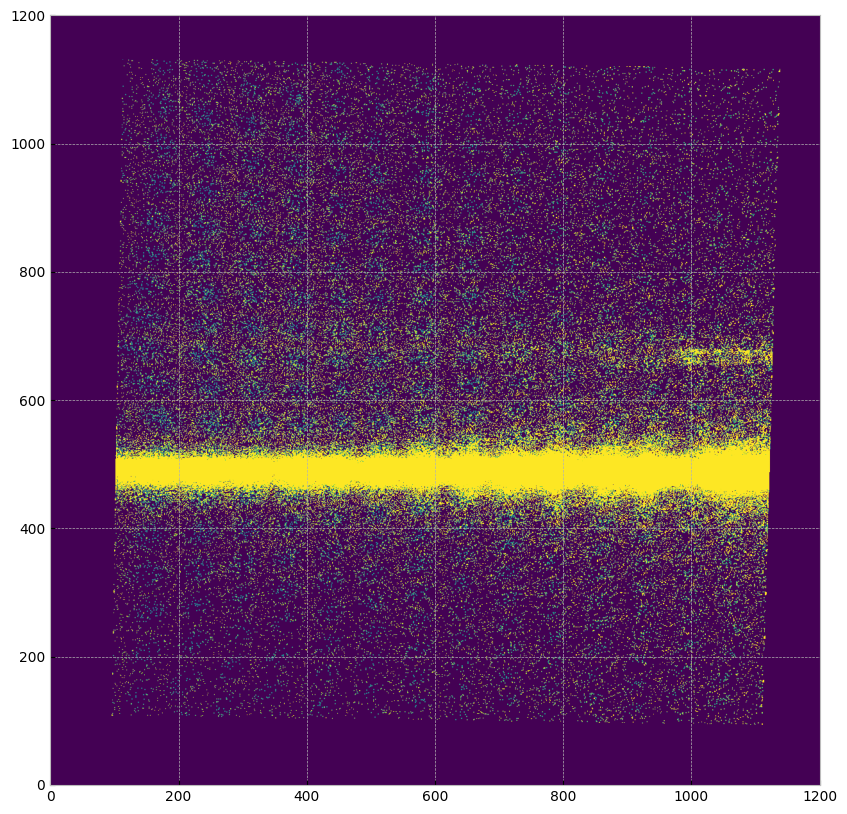
5.2 Showing the image

Now we collect the science image data from the fits file and show the image.

# get data as a numpy array
with fits.open(x2d_file) as hdu_list:
    x2d_data = hdu_list[1].data

Make a histogram of the magnitude of the image data so that we have a general idea on the distribution. Knowing the distribution is essential for us to normalize the data when showing the image.

# remove infinities and NaNs from the data when making the histogram
filtered_data = [v for row in np.log10(x2d_data) for v in row if not (np.isinf(v) or np.isnan(v))]

fig, ax = plt.subplots(1, 1)
fig.set_size_inches(15, 5)

ax.hist(filtered_data, range=[-20.5, -8.5], bins=12)
ax.set_xlabel('Magnitude order of _x2d image data')
ax.set_ylabel('count')
ax.set_title('_x2d Data Magnitude Order frequencies')

/tmp/ipykernel_1971/3318306081.py:2: RuntimeWarning: divide by zero encountered in log10
  filtered_data = [v for row in np.log10(x2d_data) for v in row if not (np.isinf(v) or np.isnan(v))]
/tmp/ipykernel_1971/3318306081.py:2: RuntimeWarning: invalid value encountered in log10
  filtered_data = [v for row in np.log10(x2d_data) for v in row if not (np.isinf(v) or np.isnan(v))]

Text(0.5, 1.0, '_x2d Data Magnitude Order frequencies')

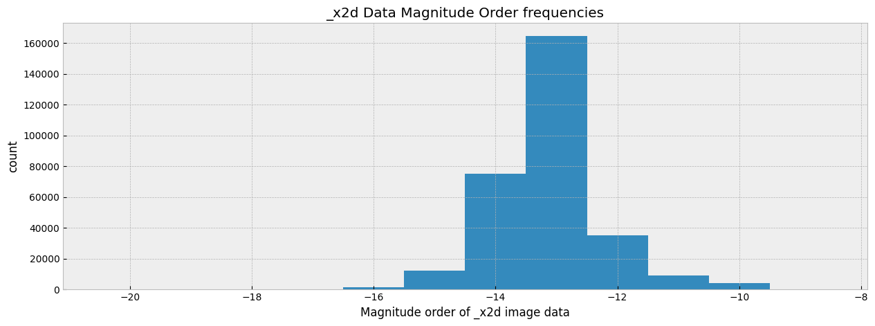
When showing the image, we normalize the color of each pixel to a specific range through vmin and vmax to make the features of image clear. These values typically matches the magnitude of the x2d data according to the histogram above, but can be experimented and changed to bring out features at different levels.

# show the image
matplotlib.rcParams['figure.figsize'] = (10, 10)
plt.imshow(x2d_data, origin='lower', vmin=0, vmax=1e-13, cmap="viridis")

<matplotlib.image.AxesImage at 0x7fb61cce93d0>

For more color map and normalizing options, see: Choosing Colormaps in Matplotlib, matplotlib.pyplot.imshow.

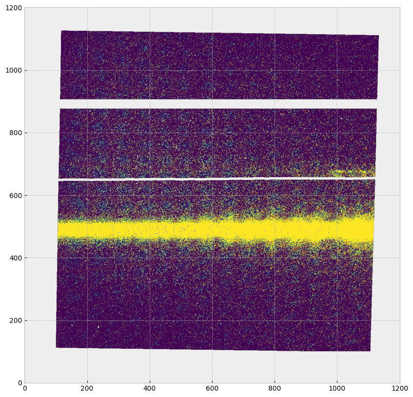
5.3 Removing serious data quality pixels

Now we are going to remove the pixels with series data quality flags as described above. The removed pixels will appear grey like the background. The horizontal stripes of removed data are from the bar (top) and repeller wire shadow (middle).

# get the serious data quality flag
sdqFlags_fuv = fits.getheader(x2d_file, 1)["SDQFLAGS"]
# get data quality flags of each pixels
with fits.open(x2d_file) as hdu_list:
    x2d_dq = hdu_list[3].data
    
    
# create a mask of bad pixels and set them to nan
def check_dq(dq):
    return bool(dq & sdqFlags_fuv)


mask = np.vectorize(check_dq)(x2d_dq)
x2d_mask = np.ma.array(x2d_data, mask=mask, fill_value=np.nan)
# plot the image
plt.imshow(x2d_mask, origin='lower', vmin=0, vmax=1e-13, cmap="viridis")

<matplotlib.image.AxesImage at 0x7fb61cce1310>

6.Working with Time-Tag data

The MAMA detecters have a unique Time-Tag mode besides ACCUM mode. TIME-TAG mode is used for high-time-resolution spectroscopy and imaging in the UV. In TIME-TAG mode, the position and detection time of every photon is recorded in an event list. The Time-Tag mode operation for the MAMA detectors can be found at: MAMA TIME-TAG Mode.

In TIME-TAG mode, the position and detection time of every photon is recorded in an event list. First download the _tag data:

# Search target objscy by obs_id
target = Observations.query_criteria(obs_id='odgxt9010')
# get a list of files assiciated with that target
NUV_list = Observations.get_product_list(target)
# Download only the SCIENCE fits files
Observations.download_products(NUV_list, extension='fits', download_dir=str(datadir))

Downloading URL https://mast.stsci.edu/api/v0.1/Download/file?uri=mast:HST/product/odgxt9010_wav.fits to data/mastDownload/HST/odgxt9010/odgxt9010_wav.fits ...

 [Done]

Downloading URL https://mast.stsci.edu/api/v0.1/Download/file?uri=mast:HST/product/odgxt9010_jwt.fits to data/mastDownload/HST/odgxt9010/odgxt9010_jwt.fits ...

 [Done]

Downloading URL https://mast.stsci.edu/api/v0.1/Download/file?uri=mast:HST/product/odgxt9010_spt.fits to data/mastDownload/HST/odgxt9010/odgxt9010_spt.fits ...

 [Done]

Downloading URL https://mast.stsci.edu/api/v0.1/Download/file?uri=mast:HST/product/odgxt9010_asn.fits to data/mastDownload/HST/odgxt9010/odgxt9010_asn.fits ...

 [Done]

Downloading URL https://mast.stsci.edu/api/v0.1/Download/file?uri=mast:HST/product/odgxt9010_raw.fits to data/mastDownload/HST/odgxt9010/odgxt9010_raw.fits ...

 [Done]

Downloading URL https://mast.stsci.edu/api/v0.1/Download/file?uri=mast:HST/product/odgxt9010_tag.fits to data/mastDownload/HST/odgxt9010/odgxt9010_tag.fits ...

 [Done]

Downloading URL https://mast.stsci.edu/api/v0.1/Download/file?uri=mast:HST/product/odgxt9010_trl.fits to data/mastDownload/HST/odgxt9010/odgxt9010_trl.fits ...

 [Done]

Downloading URL https://mast.stsci.edu/api/v0.1/Download/file?uri=mast:HST/product/odgxt9010_x1d.fits to data/mastDownload/HST/odgxt9010/odgxt9010_x1d.fits ...

 [Done]

Downloading URL https://mast.stsci.edu/api/v0.1/Download/file?uri=mast:HST/product/odgxt9010_jit.fits to data/mastDownload/HST/odgxt9010/odgxt9010_jit.fits ...

 [Done]

Downloading URL https://mast.stsci.edu/api/v0.1/Download/file?uri=mast:HST/product/odgxt9010_wsp.fits to data/mastDownload/HST/odgxt9010/odgxt9010_wsp.fits ...

 [Done]

Downloading URL https://mast.stsci.edu/api/v0.1/Download/file?uri=mast:HST/product/odgxt9010_jif.fits to data/mastDownload/HST/odgxt9010/odgxt9010_jif.fits ...

 [Done]

Downloading URL https://mast.stsci.edu/api/v0.1/Download/file?uri=mast:HST/product/odgxt9010_x2d.fits to data/mastDownload/HST/odgxt9010/odgxt9010_x2d.fits ...

 [Done]

Downloading URL https://mast.stsci.edu/api/v0.1/Download/file?uri=mast:HST/product/odgxt9010_jwf.fits to data/mastDownload/HST/odgxt9010/odgxt9010_jwf.fits ...

 [Done]

Downloading URL https://mast.stsci.edu/api/v0.1/Download/file?uri=mast:HST/product/odgxt9010_flt.fits to data/mastDownload/HST/odgxt9010/odgxt9010_flt.fits ...

 [Done]

Downloading URL https://mast.stsci.edu/api/v0.1/Download/file?uri=mast:HST/product/hasp/hst_15070_stis_v-t-cra_g230m_odgx_cspec.fits to data/mastDownload/HST/hst_hasp_15070_stis_v-t-cra_odgx/hst_15070_stis_v-t-cra_g230m_odgx_cspec.fits ...

 [Done]

Downloading URL https://mast.stsci.edu/api/v0.1/Download/file?uri=mast:HST/product/hasp/hst_15070_stis_v-t-cra_g230m_odgx09_cspec.fits to data/mastDownload/HST/hst_hasp_15070_stis_v-t-cra_odgx/hst_15070_stis_v-t-cra_g230m_odgx09_cspec.fits ...

 [Done]

Downloading URL https://mast.stsci.edu/api/v0.1/Download/file?uri=mast:HST/product/hasp/hst_15070_stis_v-t-cra_g230m_odgxc9_cspec.fits to data/mastDownload/HST/hst_hasp_15070_stis_v-t-cra_odgx/hst_15070_stis_v-t-cra_g230m_odgxc9_cspec.fits ...

 [Done]

Downloading URL https://mast.stsci.edu/api/v0.1/Download/file?uri=mast:HST/product/hasp/hst_15070_stis_v-t-cra_g230m_odgxt9_cspec.fits to data/mastDownload/HST/hst_hasp_15070_stis_v-t-cra_odgx/hst_15070_stis_v-t-cra_g230m_odgxt9_cspec.fits ...

 [Done]

Downloading URL https://mast.stsci.edu/api/v0.1/Download/file?uri=mast:HST/product/hasp/hst_15070_cos-stis_v-t-cra_g130m-g160m-g230m_ldgx_cspec.fits to data/mastDownload/HST/hst_hasp_15070_cos-stis_v-t-cra_ldgx/hst_15070_cos-stis_v-t-cra_g130m-g160m-g230m_ldgx_cspec.fits ...

 [Done]

Downloading URL https://mast.stsci.edu/api/v0.1/Download/file?uri=mast:HST/product/hasp/hst_15070_cos-stis_v-t-cra_g130m-g230m_ldgx_cspec.fits to data/mastDownload/HST/hst_hasp_15070_cos-stis_v-t-cra_ldgx/hst_15070_cos-stis_v-t-cra_g130m-g230m_ldgx_cspec.fits ...

 [Done]

Table length=20

Local Path	Status	Message	URL
str119	str8	object	object
data/mastDownload/HST/odgxt9010/odgxt9010_wav.fits	COMPLETE	None	None
data/mastDownload/HST/odgxt9010/odgxt9010_jwt.fits	COMPLETE	None	None
data/mastDownload/HST/odgxt9010/odgxt9010_spt.fits	COMPLETE	None	None
data/mastDownload/HST/odgxt9010/odgxt9010_asn.fits	COMPLETE	None	None
data/mastDownload/HST/odgxt9010/odgxt9010_raw.fits	COMPLETE	None	None
data/mastDownload/HST/odgxt9010/odgxt9010_tag.fits	COMPLETE	None	None
data/mastDownload/HST/odgxt9010/odgxt9010_trl.fits	COMPLETE	None	None
data/mastDownload/HST/odgxt9010/odgxt9010_x1d.fits	COMPLETE	None	None
data/mastDownload/HST/odgxt9010/odgxt9010_jit.fits	COMPLETE	None	None
data/mastDownload/HST/odgxt9010/odgxt9010_wsp.fits	COMPLETE	None	None
data/mastDownload/HST/odgxt9010/odgxt9010_jif.fits	COMPLETE	None	None
data/mastDownload/HST/odgxt9010/odgxt9010_x2d.fits	COMPLETE	None	None
data/mastDownload/HST/odgxt9010/odgxt9010_jwf.fits	COMPLETE	None	None
data/mastDownload/HST/odgxt9010/odgxt9010_flt.fits	COMPLETE	None	None
data/mastDownload/HST/hst_hasp_15070_stis_v-t-cra_odgx/hst_15070_stis_v-t-cra_g230m_odgx_cspec.fits	COMPLETE	None	None
data/mastDownload/HST/hst_hasp_15070_stis_v-t-cra_odgx/hst_15070_stis_v-t-cra_g230m_odgx09_cspec.fits	COMPLETE	None	None
data/mastDownload/HST/hst_hasp_15070_stis_v-t-cra_odgx/hst_15070_stis_v-t-cra_g230m_odgxc9_cspec.fits	COMPLETE	None	None
data/mastDownload/HST/hst_hasp_15070_stis_v-t-cra_odgx/hst_15070_stis_v-t-cra_g230m_odgxt9_cspec.fits	COMPLETE	None	None
data/mastDownload/HST/hst_hasp_15070_cos-stis_v-t-cra_ldgx/hst_15070_cos-stis_v-t-cra_g130m-g160m-g230m_ldgx_cspec.fits	COMPLETE	None	None
data/mastDownload/HST/hst_hasp_15070_cos-stis_v-t-cra_ldgx/hst_15070_cos-stis_v-t-cra_g130m-g230m_ldgx_cspec.fits	COMPLETE	None	None

6.1 Investigating the _tag data

# get info about the tag extension fits file
tag = Path("./data/mastDownload/HST/odgxt9010/odgxt9010_tag.fits")
fits.info(tag)

Filename: data/mastDownload/HST/odgxt9010/odgxt9010_tag.fits
No.    Name      Ver    Type      Cards   Dimensions   Format
  0  PRIMARY       1 PrimaryHDU     218   ()      
  1  EVENTS        1 BinTableHDU    148   4802131R x 4C   [1J, 1I, 1I, 1I]   
  2  GTI           1 BinTableHDU     22   1R x 2C   [1D, 1D]   

The _tag fits file has two binary table extensions: EVENTS and GTI (Good Time Interval).

# get header of the EVENTS extension
# print only the TIMETAG EVENTS TABLE COLUMNS (line 130-147)
fits.getheader(tag, 1)[130:147]

SHIFTA2 =             0.000000 / Spectrum shift in AXIS2 calculated from WAVECAL
                                                                                
              / TIMETAG EVENTS TABLE COLUMNS                                    
                                                                                
TTYPE1  = 'TIME    '           / event clock time                               
TFORM1  = '1J      '           / data format for TIME: 32-bit integer           
TUNIT1  = 'seconds '           / units for TIME: seconds                        
TSCAL1  =             0.000125 / scale factor to convert s/c clock ticks to sec 
TZERO1  =                  0.0 / TIME zero point: starting time of obs.         
TTYPE2  = 'AXIS1   '           / Doppler corrected axis 1 detector coordinate   
TFORM2  = '1I      '           / data format for AXIS1: 16-bit integer          
TUNIT2  = 'pixels  '           / physical units for AXIS1: pixels               
TTYPE3  = 'AXIS2   '           / axis 2 detector coordinate                     
TFORM3  = '1I      '           / data format for AXIS2: 16-bit integer          
TUNIT3  = 'pixels  '           / physical units for AXIS2: pixels               
TTYPE4  = 'DETAXIS1'           / raw 1 detector coordinate                      
TFORM4  = '1I      '           / data format for DETAXIS1: 16-bit integer       

Columns in the EVENTS extension:

• TIME: the time each event was recorded relative to the start time

• AXIS1: pixel coordinate along the spectral axis with the corretion term on Doppler shifts

• AXIS2: pixel coordinate along the spatial axis

• DETAXIS1: pixel coordinate along the spectral axis without the corretion term on Doppler shifts

# get header of the GTI extension
fits.getheader(tag, 2)

XTENSION= 'BINTABLE'           / extension type                                 
BITPIX  =                    8 / bits per data value                            
NAXIS   =                    2 / number of data axes                            
NAXIS1  =                   16 / length of first data axis                      
NAXIS2  =                    1 / length of second data axis                     
PCOUNT  =                    0 / number of group parameters                     
GCOUNT  =                    1 / number of groups                               
TFIELDS =                    2 / number of fields in each table row             
INHERIT =                    T / inherit the primary header                     
EXTNAME = 'GTI     '           / extension name                                 
EXTVER  =                    1 / extension version number                       
ROOTNAME= 'odgxt9010                         ' / rootname of the observation set
EXPNAME = 'odgxt9rfq                ' / exposure identifier                     
                                                                                
              / TIMETAG GTI TABLE COLUMN DESCRIPTORS                            
                                                                                
TTYPE1  = 'START   '           / start of good time interval                    
TFORM1  = '1D      '           / data format for START: REAL*8                  
TUNIT1  = 'seconds '           / physical units for START                       
TTYPE2  = 'STOP    '           / end of good time interval                      
TFORM2  = '1D      '           / data format for STOP: REAL*8                   
TUNIT2  = 'seconds '           / physical units for STOP                        

Table.read(tag, 2)

WARNING: UnitsWarning: 'seconds' did not parse as fits unit: At col 0, Unit 'seconds' not supported by the FITS standard.  If this is meant to be a custom unit, define it with 'u.def_unit'. To have it recognized inside a file reader or other code, enable it with 'u.add_enabled_units'. For details, see https://docs.astropy.org/en/latest/units/combining_and_defining.html [astropy.units.core]

Table length=1

START	STOP
seconds	seconds
float64	float64
0.022625	2380.222

Columns in the GTI extension:

• START: start of good time interval

• STOP: end of good time interval

Now we make a time series plot of the total flux over all wavelengths to see how the flux changes over the time interval:

# read the events data as a pandas dataframe for easier manipulation
events = Table.read(tag, 1).to_pandas()
# get the good time interval from the GTI extension
start, stop = Table.read(tag, 2)["START"], Table.read(tag, 2)["STOP"]
# group the events by time with bin = 3 seconds
time = np.arange(int(start), int(stop), 3)
ind = np.digitize(events['TIME'], time)
total_flux = events.groupby(ind).count()["TIME"]
# plot the flux as a function of time
# notice here that the unit of flux is counts since we are counting the number of events in a time series
matplotlib.rcParams['figure.figsize'] = (20, 7)
plt.plot(time, total_flux, marker=".", mfc="w")
plt.xlabel("Time [s]")
plt.ylabel("Total Flux [counts]")

WARNING: UnitsWarning: 'pixels' did not parse as fits unit: At col 0, Unit 'pixels' not supported by the FITS standard. Did you mean pixel? If this is meant to be a custom unit, define it with 'u.def_unit'. To have it recognized inside a file reader or other code, enable it with 'u.add_enabled_units'. For details, see https://docs.astropy.org/en/latest/units/combining_and_defining.html [astropy.units.core]
WARNING: UnitsWarning: 'seconds' did not parse as fits unit: At col 0, Unit 'seconds' not supported by the FITS standard.  If this is meant to be a custom unit, define it with 'u.def_unit'. To have it recognized inside a file reader or other code, enable it with 'u.add_enabled_units'. For details, see https://docs.astropy.org/en/latest/units/combining_and_defining.html [astropy.units.core]

Text(0, 0.5, 'Total Flux [counts]')

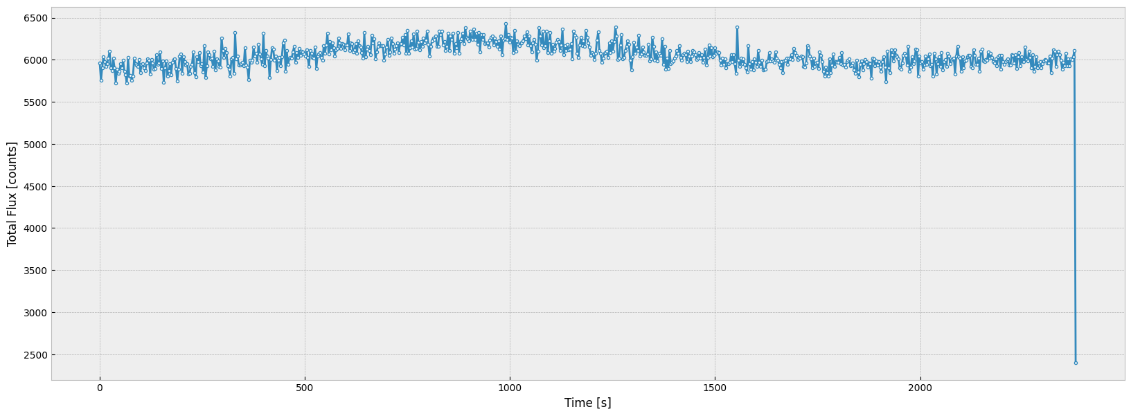
As the plot shows, though the total flux fluctuates, it is roughly a constant over the good time interval.

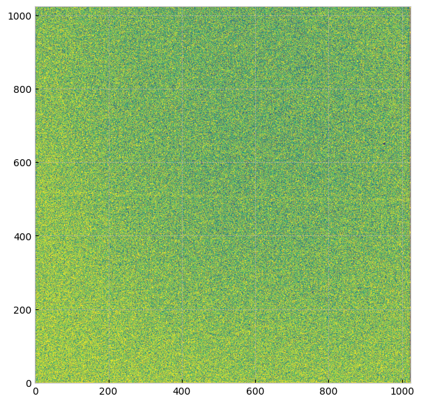
6.2 Converting Time_Tag into ACCUM image

Time tag data can be converted into ACCUM image using the inttag method in stistools. More information: inttag

# define the output file
accum = "./data/mastDownload/HST/odgxt9010/odgxt9010_accum.fits"
# convert Time_Tag into ACCUM
# the first parameter is the path to the _tag fits file, the second parameter is the output directory
stistools.inttag.inttag(tag, accum)

imset: 1, start: 0.022625, stop: 2380.222, exposure time: 2380.199375

Then the output file is in the same structure as a STIS image fits file, which we can open and plot in the same way we explored above:

with fits.open(accum) as hdul:
    im = hdul[1].data
plt.imshow(im, origin='lower', vmin=0, vmax=6, cmap="viridis")

<matplotlib.image.AxesImage at 0x7fb6198b9310>

inttag can be run to produce multiple output imsets: rcount specifies the number of imsets, imcrements specifies the time interval for each imsets in seconds

stistools.inttag.inttag(tag, accum, rcount=3, increment=700)
fits.info(accum)

imset: 1, start: 0.022625, stop: 700.022625, exposure time: 700.0

imset: 2, start: 700.022625, stop: 1400.022625, exposure time: 700.0000000000001

imset: 3, start: 1400.022625, stop: 2100.022625, exposure time: 700.0

Filename: ./data/mastDownload/HST/odgxt9010/odgxt9010_accum.fits
No.    Name      Ver    Type      Cards   Dimensions   Format
  0  PRIMARY       1 PrimaryHDU     218   ()      
  1  SCI           1 ImageHDU       139   (1024, 1024)   float64   
  2  ERR           1 ImageHDU       139   (1024, 1024)   float64   
  3  DQ            1 ImageHDU       140   ()      
  4  SCI           2 ImageHDU       139   (1024, 1024)   float64   
  5  ERR           2 ImageHDU       139   (1024, 1024)   float64   
  6  DQ            2 ImageHDU       140   ()      
  7  SCI           3 ImageHDU       139   (1024, 1024)   float64   
  8  ERR           3 ImageHDU       139   (1024, 1024)   float64   
  9  DQ            3 ImageHDU       140   ()      

Compare the 3 accum images produced by inttag, using the same scale and colormap:

for i in range(1, 8, 3):
    with fits.open(accum) as hdul:
        im = hdul[i].data
    plt.subplot(1, 3, int(i/3)+1)
    plt.imshow(im, origin='lower', vmin=0, vmax=2, cmap="viridis")
    plt.title("extension {}".format(i))
plt.tight_layout()

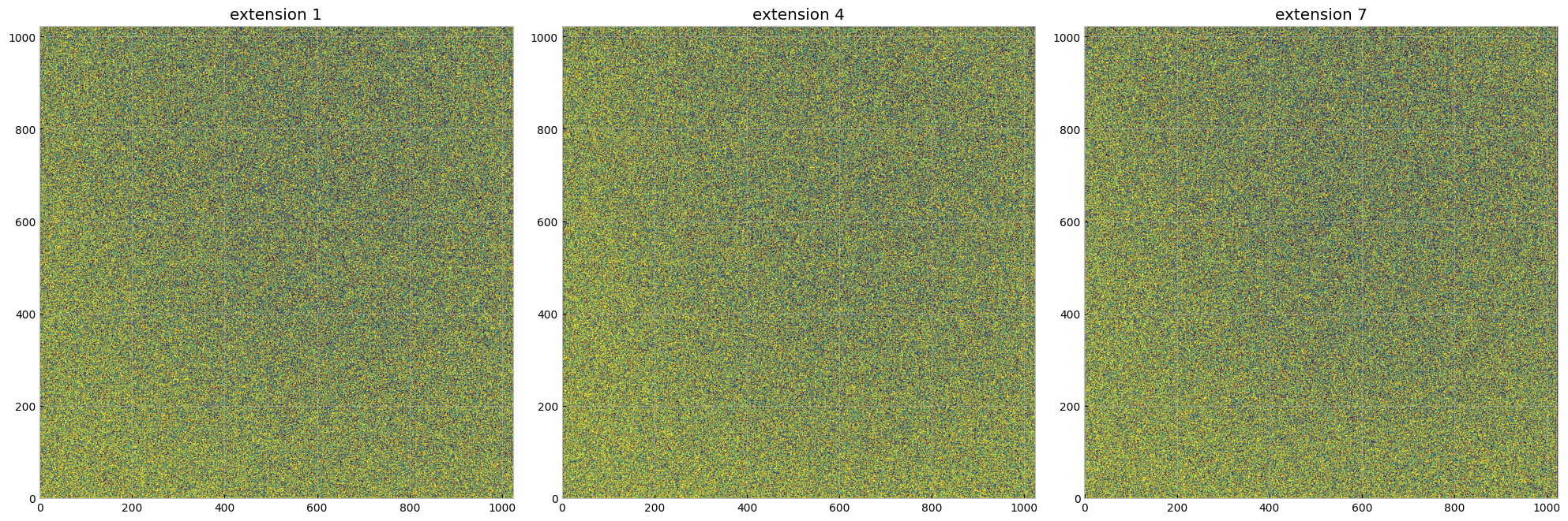
The output file is a series of extensions with each imset having a SCI, ERR, and DQ extension, as shown above.

7.Working with STIS Echelle data

The STIS Echelle mode uses diffraction and interference to separate a spectrum into different spectral orders (the keyword in the headers is SPORDER), with each spectral order covering different wavelength range. The echelle were designed to maximize the spectral range covered in a single echellogram. For more information, see Echelle Spectroscopy in the Ultraviolet.

We first download data taken with an echelle:

# Search target objscy by obs_id
target = Observations.query_criteria(obs_id='OCTX01030')
# get a list of files assiciated with that target
NUV_list = Observations.get_product_list(target)
# Download only the SCIENCE fits files
Observations.download_products(NUV_list, productType="SCIENCE", extension='fits', download_dir=str(datadir))

Downloading URL https://mast.stsci.edu/api/v0.1/Download/file?uri=mast:HST/product/octx01030_raw.fits to data/mastDownload/HST/octx01030/octx01030_raw.fits ...

 [Done]

Downloading URL https://mast.stsci.edu/api/v0.1/Download/file?uri=mast:HST/product/octx01030_flt.fits to data/mastDownload/HST/octx01030/octx01030_flt.fits ...

 [Done]

Downloading URL https://mast.stsci.edu/api/v0.1/Download/file?uri=mast:HST/product/octx01030_x1d.fits to data/mastDownload/HST/octx01030/octx01030_x1d.fits ...

 [Done]

Downloading URL https://mast.stsci.edu/api/v0.1/Download/file?uri=mast:HST/product/hasp/hst_14094_stis_-rho-cnc_e230m_octx03_cspec.fits to data/mastDownload/HST/hst_hasp_14094_stis_-rho-cnc_octx/hst_14094_stis_-rho-cnc_e230m_octx03_cspec.fits ...

 [Done]

Downloading URL https://mast.stsci.edu/api/v0.1/Download/file?uri=mast:HST/product/hasp/hst_14094_stis_-rho-cnc_e230m_octx_cspec.fits to data/mastDownload/HST/hst_hasp_14094_stis_-rho-cnc_octx/hst_14094_stis_-rho-cnc_e230m_octx_cspec.fits ...

 [Done]

Downloading URL https://mast.stsci.edu/api/v0.1/Download/file?uri=mast:HST/product/hasp/hst_14094_stis_-rho-cnc_e230m_octx01_cspec.fits to data/mastDownload/HST/hst_hasp_14094_stis_-rho-cnc_octx/hst_14094_stis_-rho-cnc_e230m_octx01_cspec.fits ...

 [Done]

Downloading URL https://mast.stsci.edu/api/v0.1/Download/file?uri=mast:HST/product/hasp/hst_14094_cos-stis_-rho-cnc_g130m-e230m_lctx_cspec.fits to data/mastDownload/HST/hst_hasp_14094_cos-stis_-rho-cnc_lctx/hst_14094_cos-stis_-rho-cnc_g130m-e230m_lctx_cspec.fits ...

 [Done]

Table length=7

Local Path	Status	Message	URL
str115	str8	object	object
data/mastDownload/HST/octx01030/octx01030_raw.fits	COMPLETE	None	None
data/mastDownload/HST/octx01030/octx01030_flt.fits	COMPLETE	None	None
data/mastDownload/HST/octx01030/octx01030_x1d.fits	COMPLETE	None	None
data/mastDownload/HST/hst_hasp_14094_stis_-rho-cnc_octx/hst_14094_stis_-rho-cnc_e230m_octx03_cspec.fits	COMPLETE	None	None
data/mastDownload/HST/hst_hasp_14094_stis_-rho-cnc_octx/hst_14094_stis_-rho-cnc_e230m_octx_cspec.fits	COMPLETE	None	None
data/mastDownload/HST/hst_hasp_14094_stis_-rho-cnc_octx/hst_14094_stis_-rho-cnc_e230m_octx01_cspec.fits	COMPLETE	None	None
data/mastDownload/HST/hst_hasp_14094_cos-stis_-rho-cnc_lctx/hst_14094_cos-stis_-rho-cnc_g130m-e230m_lctx_cspec.fits	COMPLETE	None	None

7.1 Showing Echelle Image

Open the _flt (Flat-fielded science) image in the same way we open other image files, and show the image:

flt_file = "./data/mastDownload/HST/octx01030/octx01030_flt.fits"
with fits.open(flt_file) as hdu:
    image = hdu[1].data
    plt.imshow(image, origin='lower', vmin=0, vmax=1, cmap="viridis")

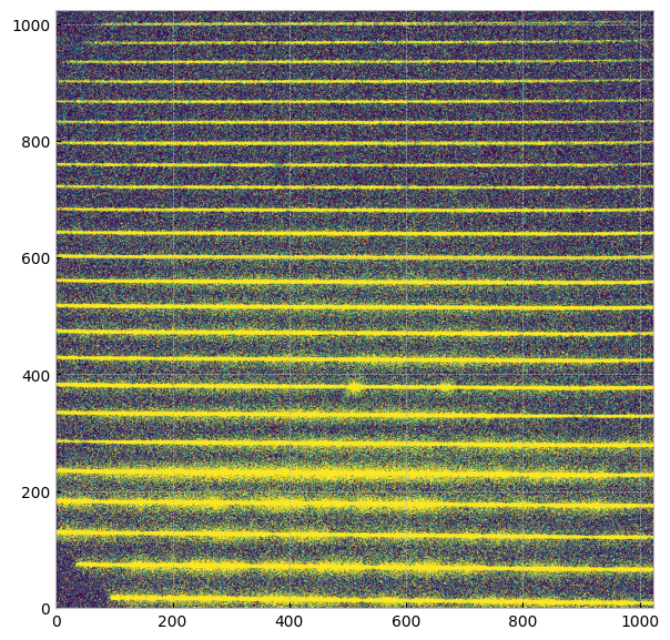
As shown in the image above, there are multiple horizontal bands with different spectral orders. Each spectral order also has distinct wavelength range, which we will explore in the next section.

7.2 Plotting Echelle Spectrum

We first read in the _x1d data as an astropy table. Notice that when we read in the FUV _x1d data in section2.2, the table has a single row with SPORDER = 1. But for echelle mode data, the data is separated into multiple rows, with each row having a distinct order.

echelle_file = "./data/mastDownload/HST/octx01030/octx01030_x1d.fits"
echelle_data = Table.read(echelle_file, 1)
echelle_data

WARNING: UnitsWarning: 'Angstroms' did not parse as fits unit: At col 0, Unit 'Angstroms' not supported by the FITS standard. Did you mean Angstrom or angstrom? If this is meant to be a custom unit, define it with 'u.def_unit'. To have it recognized inside a file reader or other code, enable it with 'u.add_enabled_units'. For details, see https://docs.astropy.org/en/latest/units/combining_and_defining.html [astropy.units.core]
WARNING: UnitsWarning: 'Counts/s' did not parse as fits unit: At col 0, Unit 'Counts' not supported by the FITS standard. Did you mean count? If this is meant to be a custom unit, define it with 'u.def_unit'. To have it recognized inside a file reader or other code, enable it with 'u.add_enabled_units'. For details, see https://docs.astropy.org/en/latest/units/combining_and_defining.html [astropy.units.core]
WARNING: UnitsWarning: 'erg/s/cm**2/Angstrom' contains multiple slashes, which is discouraged by the FITS standard [astropy.units.format.generic]

Table length=24

SPORDER	NELEM	WAVELENGTH	GROSS	BACKGROUND	NET	FLUX	ERROR	NET_ERROR	DQ	A2CENTER	EXTRSIZE	MAXSRCH	BK1SIZE	BK2SIZE	BK1OFFST	BK2OFFST	EXTRLOCY	OFFSET
		Angstroms	Counts/s	Counts/s	Counts/s	erg / (Angstrom s cm2)	erg / (Angstrom s cm2)	Counts/s		pix	pix	pix	pix	pix	pix	pix	pix	pix
int16	int16	float64[1024]	float32[1024]	float32[1024]	float32[1024]	float32[1024]	float32[1024]	float32[1024]	int16[1024]	float32	float32	int16	float32	float32	float32	float32	float32[1024]	float32
66	1024	3067.682086855123 .. 3119.012536891768	-0.0002928353 .. 0.4817821	0.006654883 .. 0.003304005	-0.006947719 .. 0.4784781	-2.030472e-14 .. 2.9376e-12	3.13553e-17 .. 4.646945e-13	1.072892e-05 .. 0.07568973	2628 .. 2564	14.40747	7	10	5	5	28.01995	-28.77343	19.45284 .. 9.476334	0.6031901
67	1024	3021.857427057288 .. 3072.451049005796	-0.0002917696 .. 0.8308571	0.004698814 .. 0.0009105802	-0.004990583 .. 0.8299465	-1.021074e-14 .. 3.076689e-12	2.202596e-17 .. 3.702814e-13	1.076537e-05 .. 0.09988457	2628 .. 2580	71.19333	7	10	5	5	27.28738	-28.01995	75.95515 .. 66.73722	0.6031901
68	1024	2977.380919809147 .. 3027.257338502545	-0.008585975 .. 0.4190482	0.01313506 .. 0.002161205	-0.02172103 .. 0.416887	-3.754732e-14 .. 1.087724e-12	1.012584e-16 .. 1.857633e-13	5.857771e-05 .. 0.07119664	2580 .. 2564	126.3683	7	10	5	5	26.57536	-27.28738	131.2862 .. 122.4106	0.6031901
69	1024	2934.193937243135 .. 2983.372006818285	-0.0003262974 .. 0.9740262	0.01347407 .. 0.002397954	-0.01380036 .. 0.9716282	-2.190875e-14 .. 2.144429e-12	1.805634e-17 .. 2.292797e-13	1.137373e-05 .. 0.1038853	2564 .. 2564	179.9044	7	10	5	5	25.88353	-26.57536	184.4561 .. 176.3899	0.5168006
70	1024	2892.241202288543 .. 2940.739046013224	-0.0003810195 .. 1.413689	0.01000194 .. 0.003849149	-0.01038296 .. 1.40984	-1.478441e-14 .. 3.037708e-12	1.750356e-17 .. 2.665483e-13	1.229259e-05 .. 0.1237086	2564 .. 2564	232.084	7	10	5	5	25.21152	-25.88353	236.3518 .. 228.9839	0.5693149
71	1024	2851.470552660116 .. 2899.305600220004	-0.0002589348 .. 1.353963	0.002504814 .. 0.005018473	-0.002763749 .. 1.348944	-3.966172e-15 .. 2.761381e-12	1.45592e-17 .. 2.479407e-13	1.014529e-05 .. 0.1211199	2564 .. 2564	282.7352	7	10	5	5	24.55895	-25.21152	286.8198 .. 280.1042	0.5335948
72	1024	2811.832724517215 .. 2859.021746954763	-0.0002629836 .. 0.3712038	0.005110647 .. 0.001835793	-0.00537363 .. 0.369368	-7.334717e-15 .. 7.610627e-13	1.40482e-17 .. 1.381501e-13	1.029212e-05 .. 0.06704865	2564 .. 2564	332.0811	7	10	5	5	23.92547	-24.55895	335.8839 .. 329.9276	0.5793937
73	1024	2773.281153907109 .. 2819.840296387559	-0.007595196 .. 0.7308141	0.005754123 .. 0.002980053	-0.01334932 .. 0.727834	-1.893139e-14 .. 1.559154e-12	7.808778e-17 .. 1.939492e-13	5.506296e-05 .. 0.09053811	2580 .. 2564	380.1232	7	10	5	5	23.31071	-23.92547	383.655 .. 378.4149	0.6563193
74	1024	2735.771794309852 .. 2781.716606874576	-0.0002480344 .. 0.3054057	0.003892346 .. 0.001905411	-0.00414038 .. 0.3035003	-6.107451e-15 .. 6.842402e-13	1.461313e-17 .. 1.387065e-13	9.906572e-06 .. 0.06152438	2564 .. 2564	426.7452	7	10	5	5	22.7143	-23.31071	430.1284 .. 425.6361	0.5977612
...	...	...	...	...	...	...	...	...	...	...	...	...	...	...	...	...	...	...
80	1024	2530.413003679701 .. 2572.968492248937	-0.0003557455 .. 0.2057582	0.0008996339 .. 0.0008307099	-0.001255379 .. 0.2049275	-2.266979e-15 .. 6.605272e-13	2.129495e-17 .. 1.840417e-13	1.179246e-05 .. 0.05709862	2564 .. 2580	682.4249	7	10	5	5	19.50066	-19.99467	684.3518 .. 683.5427	0.574106
81	1024	2499.145134209817 .. 2541.180702698945	-0.0003548819 .. 0.1215624	0.001022874 .. 0.0004910007	-0.001377756 .. 0.1210714	-2.67421e-15 .. 4.349387e-13	2.296038e-17 .. 1.542925e-13	1.182921e-05 .. 0.04294955	2564 .. 2564	721.4458	7	10	5	5	19.02243	-19.50066	723.0336 .. 722.7673	0.6433231
82	1024	2468.640092359287 .. 2510.167438601849	-0.0003482449 .. -0.003966084	0.0008586684 .. 0.000385318	-0.001206913 .. -0.004351402	-2.455758e-15 .. -1.745655e-14	2.389558e-17 .. 9.369933e-14	1.174379e-05 .. 0.02335647	2564 .. 2564	759.4905	7	10	5	5	18.55963	-19.02243	760.7408 .. 761.0947	0.6800641
83	1024	2438.870300747431 .. 2479.900734272652	-0.0003480999 .. 0.01043349	0.0008362265 .. 0.0003163153	-0.001184326 .. 0.01011717	-2.494167e-15 .. 4.517789e-14	2.477215e-17 .. 1.178575e-13	1.176277e-05 .. 0.02639309	2564 .. 2564	796.5957	7	10	5	5	18.11187	-18.55963	797.6779 .. 798.4939	0.6858787
84	1024	2409.809495426899 .. 2450.35395445196	-0.009019177 .. -0.02464523	0.0007386059 .. 0.0002919547	-0.009757783 .. -0.02493719	-2.180459e-14 .. -1.227559e-13	1.338733e-16 .. 8.824105e-14	5.990969e-05 .. 0.01792569	2580 .. 2564	832.8112	7	10	5	5	17.6788	-18.11187	833.6877 .. 835.0537	0.6772088
85	1024	2381.432648611571 .. 2421.501716113727	-0.0003795348 .. 0.01215911	0.0006555628 .. 0.0002394877	-0.001035098 .. 0.01191962	-2.473746e-15 .. 6.20382e-14	2.926687e-17 .. 1.381439e-13	1.224623e-05 .. 0.02654208	2564 .. 2564	868.1068	7	10	5	5	17.26004	-17.6788	868.6304 .. 870.5798	0.5922172
86	1024	2353.715896795153 .. 2393.319815723954	-0.001006938 .. 0.0003168302	0.0005367392 .. 0.0001913979	-0.001543677 .. 0.0001254323	-3.907116e-15 .. 7.426204e-16	5.0486e-17 .. 1.442338e-13	1.99467e-05 .. 0.02436181	2564 .. 2564	902.6919	7	10	5	5	16.85524	-17.26004	903.1175 .. 905.5428	0.610154
87	1024	2326.636473828409 .. 2365.785161512079	-0.0004271266 .. -0.03641235	0.0004190952 .. 0.0001836866	-0.0008462218 .. -0.03659604	-2.284579e-15 .. -2.450691e-13	3.48386e-17 .. 9.885516e-14	1.290443e-05 .. 0.01476199	2628 .. 2564	936.4824	7	10	5	5	16.46401	-16.85524	936.36 .. 939.4832	0.6185553
88	1024	2300.172648559522 .. 2338.875710356606	-0.0003803358 .. -0.02699966	0.000322222 .. 0.0001343358	-0.0007025579 .. -0.027134	-2.107181e-15 .. -1.893928e-13	3.685634e-17 .. 1.203252e-13	1.228832e-05 .. 0.01723879	2628 .. 2564	969.464	7	10	5	5	16.08601	-16.46401	969.1404 .. 972.7743	0.5765868
89	1024	2274.303666679877 .. 2312.570408922325	-0.0004408245 .. -0.03575523	7.672486e-05 .. 9.676442e-05	-0.0005175493 .. -0.035852	-1.849008e-15 .. -2.878802e-13	4.733922e-17 .. 1.175477e-13	1.325056e-05 .. 0.01463914	2628 .. 2564	1001.779	7	10	5	5	15.72085	-16.08601	1001.03 .. 1005.438	0.6015919

Now we can plot the spectrum of all spectral orders in one plot, with each spectral order having a distinct color:

# plot the spectrum; the color of each SPORDER is specified through a matplotlib built-in colormap
matplotlib.rcParams['figure.figsize'] = (20, 7)

for i in range(len(echelle_data)):
    plt.plot(echelle_data[i]['WAVELENGTH'], echelle_data[i]['FLUX'], color=cm.get_cmap('prism')(i/len(echelle_data)), label=echelle_data[i]['SPORDER'], alpha=0.7)
plt.xlabel('Wavelength [' + chr(197) + ']')
plt.ylabel("Flux [ergs/s/cm$^2$/" + chr(197) + "]")
plt.legend(loc='best')
plt.title("STIS Echelle Mode Spectrum")

/tmp/ipykernel_1971/1991047114.py:5: MatplotlibDeprecationWarning: The get_cmap function was deprecated in Matplotlib 3.7 and will be removed two minor releases later. Use ``matplotlib.colormaps[name]`` or ``matplotlib.colormaps.get_cmap(obj)`` instead.
  plt.plot(echelle_data[i]['WAVELENGTH'], echelle_data[i]['FLUX'], color=cm.get_cmap('prism')(i/len(echelle_data)), label=echelle_data[i]['SPORDER'], alpha=0.7)

Text(0.5, 1.0, 'STIS Echelle Mode Spectrum')

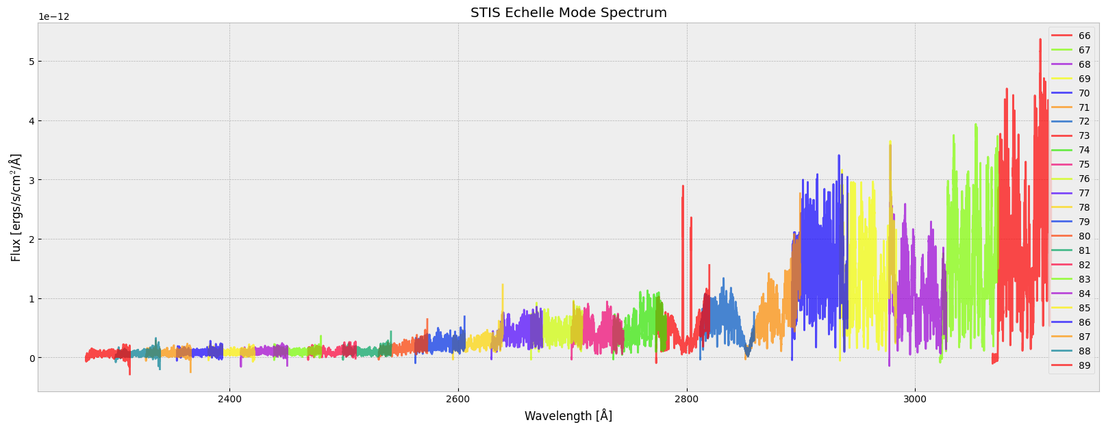
As the spectrum illustrates, each spectral order covers a specific wavelength range. Notice that some of the wavelength ranges overlap.

---

About this Notebook

Author: Keyi Ding

Updated On: 2023-01-05

This tutorial was generated to be in compliance with the STScI style guides and would like to cite the Jupyter guide in particular.

Citations

If you use astropy, matplotlib, astroquery, or numpy for published research, please cite the authors. Follow these links for more information about citations:

• Citing astropy/numpy/matplotlib

• Citing astroquery

---

Top of Page