Setting up your computer environment for working with COS data

Setting up your computer environment for working with COS data#

Learning Goals#

This Notebook is designed to walk the user (you) through:

1. Setting up a conda environment for working with COS data

- 1.1. Installing conda

- 1.2. Creating a conda environment

2. Setting up the Git repo of COS tutorials (optional)

3. Downloading up-to-date reference files

- 3.1. Downloading the most recent context

- 3.2. Downloading an older context

0. Introduction#

The Cosmic Origins Spectrograph (COS) is an ultraviolet spectrograph on-board the Hubble Space Telescope (HST) with capabilities in the near ultraviolet (NUV) and far ultraviolet (FUV).

This tutorial will walk you through setting up a Python environment for COS data analysis on your computer.

For an in-depth manual to working with COS data and a discussion of caveats and user tips, see the COS Data Handbook.
For a detailed overview of the COS instrument, see the COS Instrument Handbook.

Notes for those new to Python/Jupyter/Coding:#

You will frequently see exclamation points (!) or dollar signs ($) at the beginning of a line of code. These are not part of the actual commands. The exclamation points tell a Jupyter Notebook to pass the following line to the command line, and the dollar sign merely indicates the start of a terminal prompt.
Similarly, when a variable or argument in a line of code is surrounded by sharp brackets, like <these words are>, this is an indication that the variable or argument is something which you should change to suit your data.
If you install the full Anaconda distribution with the Anaconda Navigator tool, (see Section 1) you will also have access to a graphical interface (AKA a way to use windows and a point-and-click interface instead of the terminal for installing packages and managing environments).

Other notes:#

It is sometimes preferable to use another package manager - pip - to install necessary packages, however conda can be used to create Python environments as well as install packages. You may see both pip and conda used in these Notebooks.

1. Setting up a `conda` environment for working with COS data#

1.1. Installing `conda`#

You may already have a working conda tool. To check whether you have conda installed, open a terminal window and type conda -V, conda --version, or run the next cell. If your conda is installed and working, the terminal or cell will return the version of conda.

!conda -V

conda 24.1.2

If you receive a message that the command is unknown or not found, you must install conda. We recommend installing either the Anaconda or Minicoda distributions. See this page for instructions, and install either of the following:

Conda Distribution (with link to download)	Short Description	Size
`Anaconda` Distribution	More beginner friendly, with lots of extras you likely won’t use	~ 3 GB
`Miniconda` Distribution	Bare-bones `conda` distribution, which allows you to download only what you need	~ 400 MB
`Mamba` Distribution	Similar to `Miniconda`, rewritten in C++. Allows for faster speeds over `conda` for resolving environment dependencies.	~ 85 MB

1.2. Creating a `conda` environment#

conda allows for separate sets of packages to be installed on the same system in different environments, and for these environments to be shared so that other users can install the packages you used to get your code running. These packages are vital parts of your programming toolkit, and allow you to avoid “reinventing the wheel” by leveraging other peoples’ code. Thus, packages should be treated as any resource created by other person, and cited to avoid plagiarizing.

One package which is often necessary for working with COS data is calcos, which runs the CalCOS data pipeline. However, this package will not, by default, be installed on your computer. We will install CalCOS, as well as all the packages you will need to run any of these COS Notebooks.

Open your terminal app, likely Terminal or iTerm on a Mac or Windows Terminal or Powershell on Windows. We’ll begin by adding the conda-forge channel to conda’s channel list. This enables conda to look in the right place to find all the packages we want to install.

$ conda config --add channels conda-forge

Now we can create our new environment. We’ll call it cos_analysis_env, and initialize it with Python version 3.10.

$ conda create -n cos_analysis_env python=3.10

Allow conda to install some necessary packages (when prompted, type y then enter/return). Then, conda will need a few minutes, depending on your internet speed to complete the installation. After this installation finishes, you can see all of your environments with:

$ conda env list

Now, activate your new environment with:

$ conda activate cos_analysis_env

Note that you will need to activate your environment every time you open a new terminal or shell using conda activate cos_analysis_env. You can also do this automatically by appending conda activate cos_analysis_env to the end of your .bashrc or equivalent file. You must activate your desired conda environment before starting a Jupyter Notebook kernel in that terminal.

Finally, install CalCOS, COSTools, CRDS, and some other packages we’ll need using pip:

$ pip install calcos costools crds notebook jupyterlab matplotlib astroquery

Note that this will also likely take a few minutes to install as well.

Testing our installation#

We can test our installation by importing some of these packages. From the command line, try running:

$ python --version; python -c "import numpy, calcos, costools, crds; print('Imports succesful')"

This should return:

Python 3.10.4    # (or a similar version number)
Imports successful

Installing other packages#

We can add any other packages we need with this command:

$ pip install <first package name> <second package name> ... <last package name>

Now, go ahead and install the specutils package, which is briefly discussed in the ViewData.ipynb Notebook, using the following command:

$ pip install specutils

We’ll finish our installations by using the pip install command to download SciPy and Pandas:

pip install pandas scipy

2. Setting up the git repo of other COS tutorials (optional for some Notebooks)#

While most of the tutorial Notebooks can generally be downloaded and run independently, this is not true at present for ViewData.ipynb, which needs both the Scripts and ViewData directories installed side-by-side. For the best experience, we recommend cloning the entire repository of Notebooks.

You almost certainly have the git command line tool installed. To test it, type git --version into the command line, which should respond with a version number. If you don’t have Git installed, follow the instructions to install it here.

All of the tutorial Notebooks are hosted at this GitHub repo.

Clicking on the green “Code” button on this GitHub page gives you several options for downloading the code. Enter the directory that will store the downloaded notebooks, then copy either the https or ssh text under the Clone heading and type into your command line:

$ git clone <the text you copied> without the <>.

This will create a new directory that contains all of the tutorial notebooks you just cloned.

3. Downloading up-to-date reference files (recommended for running `CalCOS`)#

This step is suggested if you intend to process or re-process COS data using the COS calibration pipeline: CalCOS.

`CalCOS` and reference files#

The CalCOS pipeline processes science data obtained with the COS instrument using a set of reference files, such as:

Bad pixel tables to subtract off bad pixels
Flat field files to flat-field a spectrum pixel-by-pixel
Time-dependent sensitivity (TDS) tables to correct for COS’ long-term loss of sensitivity
And many more - see COS Data Handbook Section 3.4

These reference files are regularly updated by the COS team to provide the best possible calibration. The current and prior files are all hosted by the HST Calibration Reference Data System (CRDS). To get the most up-to-date COS reference files, you can use the crds command line tool which we installed in Section 1 of this Notebook.

Because some of these files are quite large, it is highly recommended you create a cache on your computer of all the COS files, which you may then update as necessary. We’ll explain how to set up that cache below.

Reference file contexts#

First we must briefly explain “contexts”: The history of reference files is stored in context files, which list the most up-to-date reference files at their time of creation.

If you wish to calibrate your data with the newest files provided by the COS team, (which is highly likely) you should download and use the files indicated by the current COS instrument context file, called an imap file. To download the files listed in the current context, see Section 3.1.
However, there are circumstances in which you may wish to use an older context, such as when you are trying to recreate the exact steps taken by another researcher. For this, see Section 3.2.
Finally, you may wish to tweak the individual reference files used, such that they don’t correspond to any particular instrument context. This is discussed in our notebook on running the CalCOS pipeline.

3.1. Downloading the most recent context#

First, we will check the CRDS website to determine what the current context is, as it changes regularly. In your browser, navigate to the HST CRDS homepage, and you will see a page as in Fig. 3.1:

Fig 3.1#

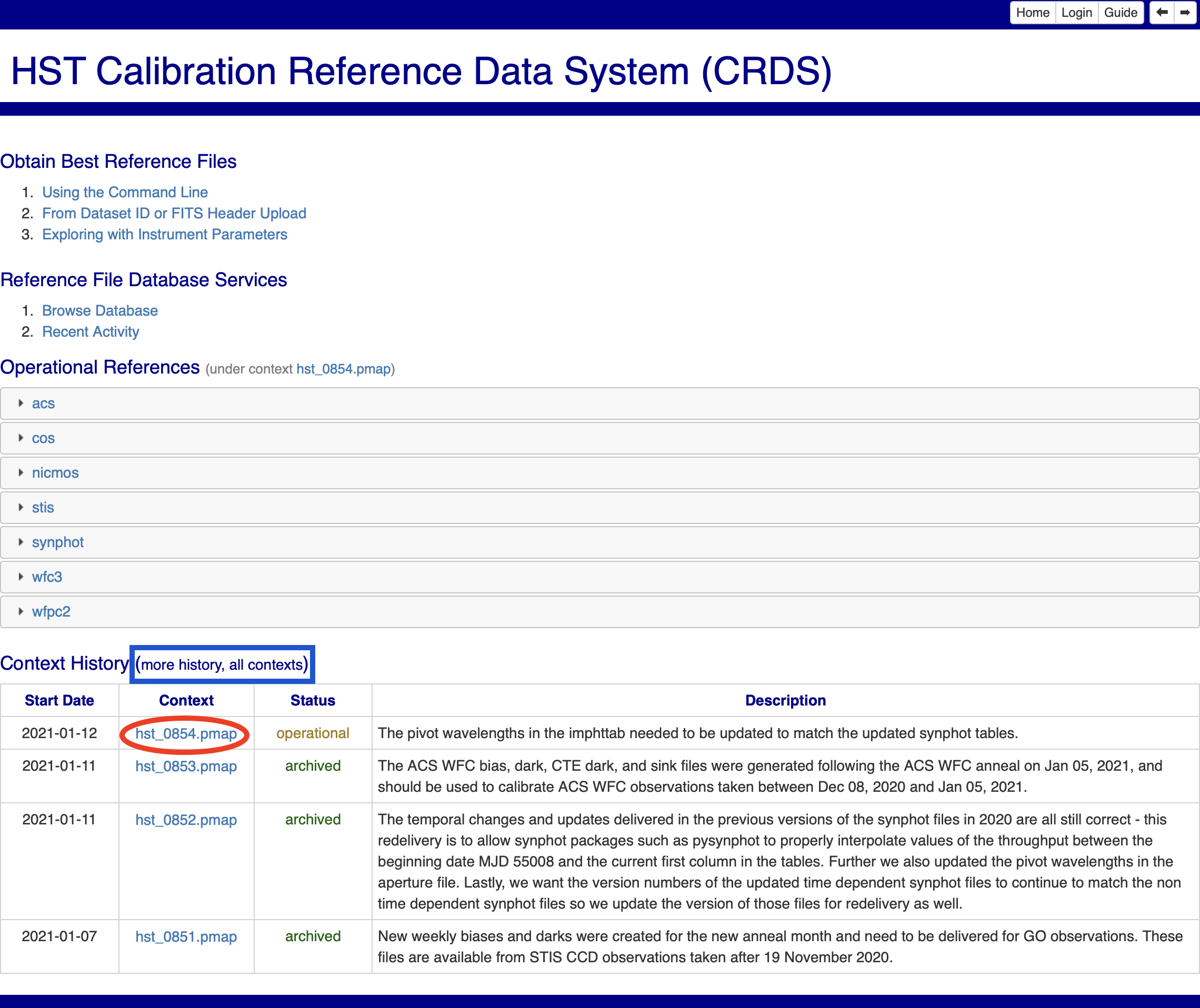
The CRDS homepage. There is a dropdown which lists all Hubble instruments. The table at the bottom of the page lists historical contexts.

At the bottom of this page is a list of recent contexts, titled “Context History”. Clicking the context listed with the Status “Operational” (circled in red in Fig 3.1) will take you to that context’s page, as shown in Fig. 3.2:

Fig 3.2#

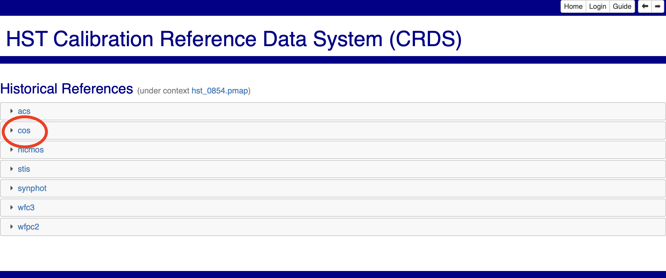
The CRDS Historical References context page on the CRDS site. Each instrument is listed on the dropdown.

Fig 3.3#

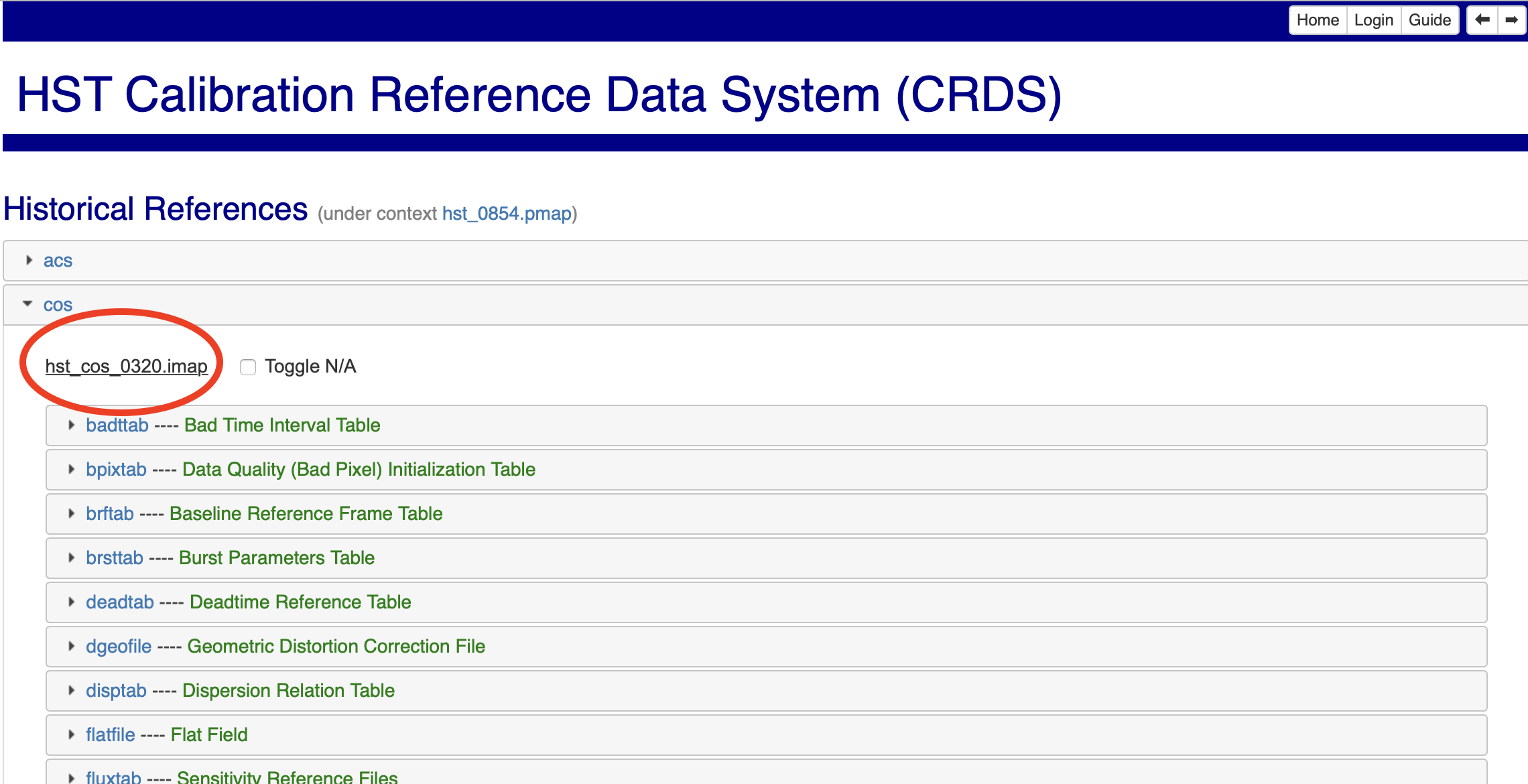
Showing the current COS context on the CRDS site. There is a large list of reference files, and the imap file labeled at the top of this list as hst_cos_0320.imap

Note down or copy the filename you just found.

The CRDS Command line tool#

Now we can download all the files in this context. Remember to first activate the conda environment you created in Section 1.2, or you may not have the necessary crds package installed.

In the next cells, we will now set several environment variables:

# First we will import OS to set environment variables
import os

We determine where to save the files on your computer. As long as you are consistent, this can be wherever you like:

# Getting your home environment
home_dir = os.environ["HOME"]

# Then we will set the CRDS_PATH environment_variable
# Creating path to where the files are saved
crds_path = os.path.join(home_dir, "crds_cache")
# Setting the environment variable CRDS_PATH to our CRDS path
os.environ["CRDS_PATH"] = crds_path

Here we are setting an environment variable to our CRDS server so we can access the files online:

# Set the CRDS_SERVER_URL environment_variable

# URL for the STScI CRDS page
crds_server_url = "https://hst-crds.stsci.edu"
# Setting env variable to URL
os.environ["CRDS_SERVER_URL"] = crds_server_url

Now we can run the initial command to sync all the files we might need. The <context number> is the last four digits of the imap filename, circled in red in Fig 3.3, without the <>. This may take from a few minutes to several hours, depending on your internet connection:

$ crds sync --contexts hst_cos_<context number>.imap --fetch-references

For running CalCOS, we recommend creating an environment variable pointing to this directory called lref.

# Set the lref environment variable
lref = os.path.join(crds_path, "references/hst/cos")
os.environ["lref"] = lref

Well done. Your reference files are now all downloaded to the cache you set up, in subdirectories for the observatory and instrument they pertain to. To see the COS reference files you just downloaded:

!ls $lref

ls: cannot access '/home/runner/crds_cache/references/hst/cos': No such file or directory

3.2. Downloading an older context#

If you know the imap context you wish to download files from, simply run the initial sync command with that context file:

$ crds sync --contexts hst_cos_<context number>.imap --fetch-references

If you instead know the observatory-wide pipeline context, (called a pmap file,) you can determine the relevant imap file by going to the “more history” or “all contexts” tabs of the CRDS website.

These pages are accessible either via the links above, or the buttons boxed in blue in Fig. 3.1. Clicking on the pmap filename and then on the cos tab will show you the cos imap filename as in Fig. 3.3. You can then run the above crds sync command with this imap file as your context.

Finally, if you instead have a FITS file of processed COS data whose context you would like to match, simply open its FITS header to find the CRDS_CTX keyword. The value for this keyword should be a pmap file, which you can search for as in the above case. Then run the above crds sync command with this imap file as your context.

Again, we recommend creating an environment variable pointing to this directory called lref:

# Set the lref environment variable
lref = os.path.join(crds_path, "references/hst/cos")
os.environ["lref"] = lref

Congratulations! You finished this Notebook!#

There are more COS data walkthrough Notebooks on different topics. You can find them here.#

About this Notebook#

Author: Nat Kerman nkerman@stsci.edu

Updated On: 2023-03-23

This tutorial was generated to be in compliance with the STScI style guides and would like to cite the Jupyter guide in particular.

Top of Page