Manual Recalibration with calwf3: Turning off the IR Linear Ramp Fit

Manual Recalibration with calwf3: Turning off the IR Linear Ramp Fit#

Learning Goals#

This notebook shows two reprocessing examples for WFC3/IR observations impacted by time-variable background (TVB).

By the end of this tutorial, you will:

Analyze exposure statistics for each read in an IMA file using pstat.
Reprocess a single exposure and an image association using calwf3.
Combine the reprocessed exposures using astrodrizzle.

Table of Contents#

Introduction
1. Imports
2. Download the data
3. Query CRDS for reference files
4. Diagnose TVB and reprocess a single exposure
5. Reprocess multiple exposures in an association
6. Conclusions
Additional Resources
About the Notebook
Citations

This notebook currently fails to execute, use as reference only

Introduction#

Exposures in the F105W and F110W filters may be impacted by Helium I emission from the Earth’s atmosphere at 1.083 microns. This typically affects the reads taken closest in time to Earth occultation. The emission produces a flat background signal which is added to the total background in a subset of reads. In some cases, this non-linear signal may be strong enough to compromise the ramp fitting performed by calwf3, which is designed to flag and remove cosmic rays and saturated reads. The affected calibrated FLT data products will have much larger noise and a non-gaussian sky background.

This notebook demonstrates how to diagnose and correct for a non-linear background and is based on the ‘Last-minus-first’ technique described in WFC3 ISR 2016-16: Reprocessing WFC3/IR Exposures Affected by Time-Variable Backgrounds. This turns off the ramp fitting step in calwf3 and treats the IR detector like a CCD that accumulates charge and is read out only at the end of the exposure. In this case, the observed count rate is determined by simply subtracting the first from the last read of the detector and dividing by the time elapsed between the two reads.

While non-linear background also impacts the IR grisms, the method described here should not be used to correct G102 and G141 observations, which are affected by a combination of Helium I, Zodiacal background, and scattered Earth light, each of which varies spatially across the detector. More detail on correcting grism data is provided in WFC3 ISR 2020-04: The dispersed infrared background in WFC3 G102 and G141 observations.

1. Imports#

This notebook assumes you have installed the required libraries as described here.

We import:

glob for finding lists of files
os for setting environment variables
shutil for managing directories
matplotlib.pyplot for plotting data
astropy.io fits for accessing FITS files
astroquery.mast Observations for downloading data from MAST
ccdproc for building the association
drizzlepac astrodrizzle for combining images
stwcs for updating the World Coordinate System
wfc3tools calwf3 and pstat for calibrating WFC3 data and plotting statistics of WFC3 data

%matplotlib inline

import glob
import os
import shutil 

import matplotlib.pyplot as plt

from astropy.io import fits
from astroquery.mast import Observations
from ccdproc import ImageFileCollection
from drizzlepac import astrodrizzle
from stwcs import updatewcs

from wfc3tools import calwf3, pstat

2. Download the data#

The following commands query MAST for the necessary products and then downloads them to the current directory. Here we obtain WFC3/IR observations from CANDELS program 12242, Visit BF. The data products requested are the ASN, RAW, IMA, FLT, and DRZ files.

Warning: this cell may take a few minutes to complete.#

data_list = Observations.query_criteria(obs_id='IBOHBF040')

Observations.download_products(
    data_list['obsid'], 
    project='CALWF3', 
    download_dir='./data', 
    mrp_only=False, 
    productSubGroupDescription=['ASN', 'RAW', 'IMA', 'FLT', 'DRZ'])

science_files = glob.glob('data/mastDownload/HST/*/*fits')

for im in science_files:
    root = os.path.basename(im)
    new_path = os.path.join('.', root)
    os.rename(im, new_path)

data_directory = './data'

try:
    if os.path.isdir(data_directory):
        shutil.rmtree(data_directory)
except Exception as e:
    print(f"An error occured while deleting the directory {data_directory}: {e}")

The association file for visit BF comprises six consecutive exposures in F105W acquired in a single visit over 3 orbits. Each orbit consists of two 1600 sec exposures, followed by the Earth occultation. Each exposure is dithered by a small fraction of the field of view, where the POSTARG values listed below are in arseconds.

image_collection = ImageFileCollection(
    './',
    keywords=[
        "asn_id",
        "targname",
        "filter",
        "samp_seq",
        "nsamp",
        "exptime",
        "postarg1",
        "postarg2",
        "date-obs",
        "time-obs",
    ], 
    glob_include="*flt.fits",
    ext=0,
)

try:
    summary_table = image_collection.summary
    if summary_table:
        print(summary_table)
    else:
        print("No FITS files matched the pattern or no relevant data found.")
except Exception as e:
    print(f"An error occurred while creating the summary table: {e}")

3. Query CRDS for reference files#

Before running calwf3, we need to set some environment variables for several subsequent calibration tasks.

We will point to a subdirectory called crds_cache/ using the IREF environment variable. The IREF variable is used for WFC3 reference files. Other instruments use other variables, e.g., JREF for ACS.

os.environ['CRDS_SERVER_URL'] = 'https://hst-crds.stsci.edu'
os.environ['CRDS_SERVER'] = 'https://hst-crds.stsci.edu'
os.environ['CRDS_PATH'] = './crds_cache'
os.environ['iref'] = './crds_cache/references/hst/wfc3/'

The code block below will query CRDS for the best reference files currently available for these datasets and update the header keywords to point to these new files. We will use the Python package os to run terminal commands. In the terminal, the line would be:

crds bestrefs --files [filename] --sync-references=1 --update-bestrefs

…where ‘filename’ is the name of your fits file.

Warning: this cell may take a few minutes to complete.#

raw_files = glob.glob('*_raw.fits')

for file in raw_files:
    command_line_input = f'crds bestrefs --files {file} --sync-references=1 --update-bestrefs'
    os.system(command_line_input)

4. Diagnose TVB and reprocess a single exposure#

In this example, we assume that the observer desires to reprocess only a single exposure with the ramp fitting step turned off. This is done by setting the CRCORR switch to OMIT from the default value (PERFORM).

First, we list the contents of the image association ‘ibohbf040’. This provides the rootnames of the six dithered exposures.

fits.getdata('ibohbf040_asn.fits', 1)

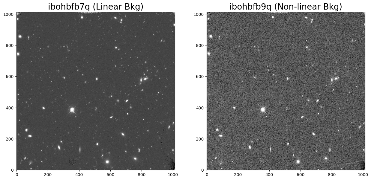
Here, we compare the first two images in the set: ‘ibohbfb7q’ and ‘ibohbfb9q’. The first is has a nominal background with a constant rate and the second has a strongly non-linear background.

b7q_data = fits.getdata('ibohbfb7q_flt.fits', ext=1)
b9q_data = fits.getdata('ibohbfb9q_flt.fits', ext=1)

fig = plt.figure(figsize=(15, 8))
ax1 = fig.add_subplot(1, 2, 1)
ax2 = fig.add_subplot(1, 2, 2)

ax1.imshow(b7q_data, vmin=0.25, vmax=1.25, cmap='Greys_r', origin='lower')
ax2.imshow(b9q_data, vmin=1.25, vmax=2.25, cmap='Greys_r', origin='lower')

ax1.set_title('ibohbfb7q (Linear Bkg)', fontsize=20)
ax2.set_title('ibohbfb9q (Non-linear Bkg)', fontsize=20)

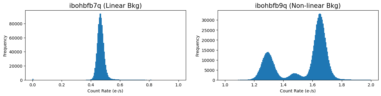
Next, we compare histograms of the two FLT frames. Exposure ‘ibohbfb9q’ has a strongly non-gaussian background with three separate peaks due to a poor ramp fit during calwf3 processing.

fig = plt.figure(figsize=(15, 3))
ax1 = fig.add_subplot(1, 2, 1)
ax2 = fig.add_subplot(1, 2, 2)

n, bins, patches = ax1.hist(b7q_data.flatten(), bins=200, range=(0, 1))
n, bins, patches = ax2.hist(b9q_data.flatten(), bins=200, range=(1, 2))

ax1.set_title('ibohbfb7q (Linear Bkg)', fontsize=15)
ax1.set_xlabel('Count Rate (e-/s)')
ax1.set_ylabel('Frequency')

ax2.set_title('ibohbfb9q (Non-linear Bkg)', fontsize=15)
ax2.set_xlabel('Count Rate (e-/s)')
ax2.set_ylabel('Frequency')

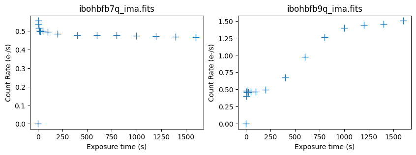
Next, we use pstat in wfc3tools to plot statistics for the individual reads in each IMA file. Here, we plot the midpoint of each read in units of count rate. For the first image, the background is relatively constant throughout the exposure at 0.5 e/s. In the second image, the background quickly increases from a value of 0.5 e/s and levels off at ~1.5 e/s toward the end of the exposure.

imafiles = ('ibohbfb7q_ima.fits', 'ibohbfb9q_ima.fits')
fig, axarr = plt.subplots(1, 2)
axarr = axarr.reshape(-1)
fig.set_size_inches(10, 3)
fig.set_dpi(100)

for i, ima in enumerate(imafiles):
    time, counts = pstat(ima, stat='midpt', units='rate', plot=False)
    axarr[i].plot(time, counts, '+', markersize=10)
    axarr[i].set_title(ima)
    axarr[i].set_xlabel('Exposure time (s)')
    axarr[i].set_ylabel('Count Rate (e-/s)')

To reprocess this image, we set the value of the header keyword CRCORR to “OMIT”. This will perform all steps in the calibration pipeline except for the ramp fitting. To see the current value of CRCORR, we use astropy.io.fits.getval( ) .

fits.getval('ibohbfb9q_raw.fits', 'CRCORR', 0)

Next, we edit the primary image header of the raw file to reflect the new value of CRCORR.

fits.setval('ibohbfb9q_raw.fits', 'CRCORR', value='OMIT')

Before running calwf3, we move the original pipeline products to a directory called orig/.

os.makedirs('orig/', exist_ok=True)

for file_pattern in ['ibohbf*_ima.fits', 'ibohbf*_flt.fits', 'ibohbf*_drz.fits']:
    for file in glob.glob(file_pattern):
        destination_path = os.path.join('orig', os.path.basename(file))
        if os.path.isfile(destination_path):
            os.remove(destination_path)
        shutil.move(file, destination_path)  

Finally, we run calwf3 on the single raw exposure.

calwf3('ibohbfb9q_raw.fits')

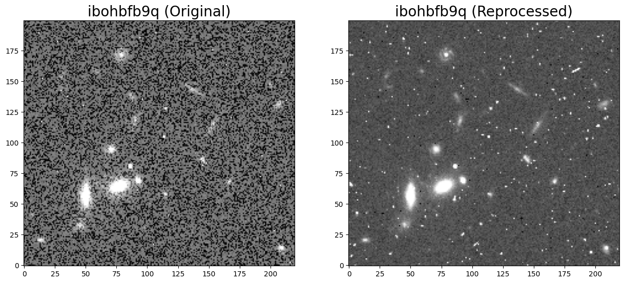
The product will be a single calibrated IMA and FLT image. We now compare the original FLT and the reprocessed FLT for a small 200x200 pixel region of the detector.

b9q_data = fits.getdata('orig/ibohbfb9q_flt.fits', ext=1)
b9q_newdata = fits.getdata('ibohbfb9q_flt.fits', ext=1)

fig = plt.figure(figsize=(15, 8))
ax1 = fig.add_subplot(1, 2, 1)
ax2 = fig.add_subplot(1, 2, 2)

ax1.imshow(b9q_data[520:720, 750:970], vmin=1.25, vmax=2.25, cmap='Greys_r', origin='lower')
ax2.imshow(b9q_newdata[520:720, 750:970], vmin=1.25, vmax=2.25, cmap='Greys_r', origin='lower')

ax1.set_title('ibohbfb9q (Original)', fontsize=20)
ax2.set_title('ibohbfb9q (Reprocessed)', fontsize=20)

Here we plot the image histogram showing the background in the original and reprocessed images.

fig = plt.figure(figsize=(15, 3))
ax1 = fig.add_subplot(1, 2, 1)
ax2 = fig.add_subplot(1, 2, 2)

n, bins, patches = ax1.hist(b9q_data.flatten(), bins=200, range=(1, 2))
n, bins, patches = ax2.hist(b9q_newdata.flatten(), bins=200, range=(1, 2))

ax1.set_title('ibohbfb9q (Original FLT)', fontsize=15)
ax1.set_xlabel('Count Rate (e-/s)')
ax1.set_ylabel('Frequency')

ax2.set_title('ibohbfb9q (Reprocessed FLT)', fontsize=15)
ax2.set_xlabel('Count Rate (e-/s)')
ax2.set_ylabel('Frequency')

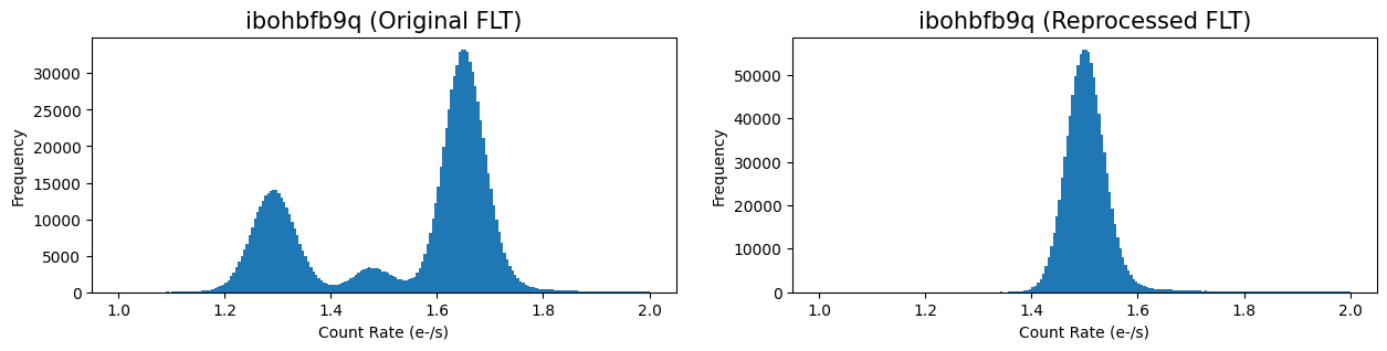
The non-gaussian image histogram is now corrected in the reprocessed FLT and the distribution is centered at a mean background of 1.5 e/s. One caveat of this approach is that cosmic-rays are not cleaned in the reprocessed image and will need to be corrected when combining the six FLT frames with AstroDrizzle. This is demonstrated in the next example.

5. Reprocess multiple exposures in an association#

In this example, we inspect the other images in the association to determine which are impacted by time-variable background, and we reprocess all six images with calwf3 and astrodrizzle.

Again, we list the contents of the association (asn) table.

dat = fits.getdata('ibohbf040_asn.fits', 1)
dat

We can also print only the rootnames (ipppssoots) in the association.

dat['MEMNAME']

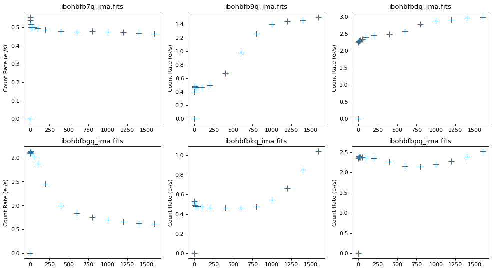
Using pstat, we can identify which of the six images are impacted by time-variable background.

Individual exposures b9q, bgq, and bkq show signs of strong time-variable background, where the change is more than a factor of 2. We will turn off the ramp fitting for these images and rerun calwf3.

imafiles = sorted(glob.glob('orig/*ima.fits'))
fig, axarr = plt.subplots(2, 3)
axarr = axarr.reshape(-1)
fig.set_size_inches(15, 8)
fig.set_dpi(80)

for i, ima in enumerate(imafiles):
    time, counts = pstat(ima, stat='midpt', units='rate', plot=False)
    axarr[i].plot(time, counts, '+', markersize=10)
    axarr[i].set_title(ima[5:], fontsize=12)
    axarr[i].set_ylabel('Count Rate (e-/s)')

Here we edit the primary image header of the three RAW images to set CRCORR to the value OMIT.

for rawfile in ['ibohbfb9q_raw.fits', 'ibohbfbgq_raw.fits', 'ibohbfbkq_raw.fits']:
    fits.setval(rawfile, 'CRCORR', value='OMIT')

Next, we remove the calibrated products from the first example and then run calwf3 on the image association.

os.remove('ibohbfb9q_ima.fits')
os.remove('ibohbfb9q_flt.fits')

calwf3('ibohbf040_asn.fits')

# Alternatively, calwf3 may be run on a list of RAW files rather than the ASN

# for raws in glob.glob('ibohbf*_raw.fits'):
#     calwf3(raws)

Finally we combine the reprocessed FLTs with AstroDrizzle.

First, the World Coordinate System (WCS) of the calibrated images must be updated using updatewcs. This prepares the image for astrodrizzle to apply the various components of geometric distortion correction.

When the parameter use_db=False, the WCS will be based on the coordinates of the Guide Star Catalogs in use at the time. No realignment of the images is performed, and this typically gives the best ‘relative’ astrometry between exposures in a visit, either in the same filter or across multiple filters.

When use_db=True, the software will connect to the astrometry database and update the WCS to an absolute frame of reference, typically based on an external catalog such as Gaia. Here, the quality of the fit is dependent on the number of bright sources in each image, and in some cased the relative astrometry may not be optimal.

for flts in glob.glob('ibohbf*_flt.fits'):
    updatewcs.updatewcs(input=flts, use_db=False)          

Next, we use AstroDrizzle to combine the FLT frames, making use of internal CR-flagging algorithms to clean the images.

astrodrizzle.AstroDrizzle(input='ibohbf040_asn.fits', mdriztab=True, preserve=False, clean=True)

The quality of the reprocessed DRZ product is significantly improved and the histogram of the background is narrower. Cosmic-rays which were present in the three reprocessed FLTs are effectively cleaned from the combined image.

drz_origdata = fits.getdata('orig/ibohbf040_drz.fits', ext=1)
drz_newdata = fits.getdata('ibohbf040_drz.fits', ext=1)

fig = plt.figure(figsize=(15, 8))
ax1 = fig.add_subplot(1, 2, 1)
ax2 = fig.add_subplot(1, 2, 2)

ax1.imshow(drz_origdata[520:720, 750:970], vmin=0.4, vmax=0.6, cmap='Greys_r', origin='lower')
ax2.imshow(drz_newdata[520:720, 750:970], vmin=0.4, vmax=0.6, cmap='Greys_r', origin='lower')

ax1.set_title('Original DRZ', fontsize=20)
ax2.set_title('Reprocessed DRZ', fontsize=20)

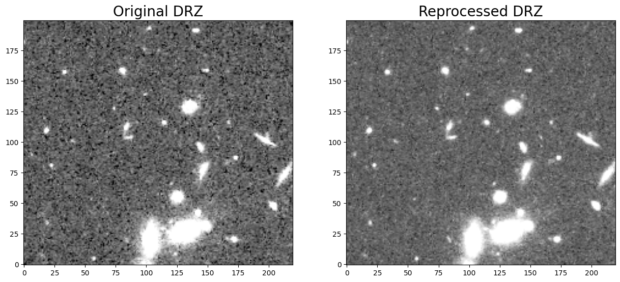
fig = plt.figure(figsize=(15, 3))
ax1 = fig.add_subplot(1, 2, 1)
ax2 = fig.add_subplot(1, 2, 2)

n, bins, patches = ax1.hist(drz_origdata.flatten(), bins=200, range=(0.4, 0.52))
n, bins, patches = ax2.hist(drz_newdata.flatten(), bins=200, range=(0.4, 0.52))

ax1.set_title('Original DRZ', fontsize=15)
ax2.set_title('Reprocessed DRZ', fontsize=15)

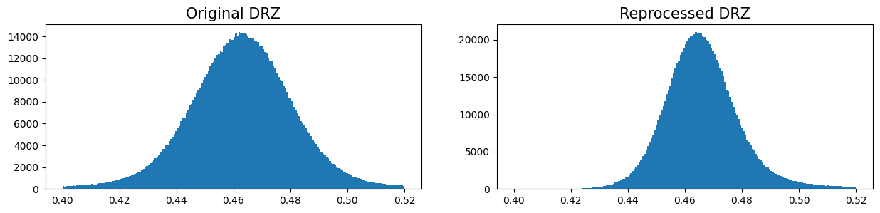
6. Conclusions#

Thank you for walking through this notebook. Now using WFC3 data, you should be more familiar with:

Analyzing exposure statistics for each read in an IMA file using pstat.
Reprocessing a single exposure and an image association using calwf3.
Combining the reprocessed exposures using astrodrizzle.

Congratulations, you have completed the notebook!#

Additional Resources#

Below are some additional resources that may be helpful. Please send any questions through the HST Helpdesk.

WFC3 Website
WFC3 Instrument Handbook
WFC3 Data Handbook
- see section 3.5.2 for reference to this notebook
- see section 7.10 for further discussion of time-variable background

About this Notebook#

Authors: Jennifer Mack, Harish Khandrika; WFC3 Instrument Team

Created on: 2021-09-13

Updated on: 2023-11-16

Source: The notebook is sourced from hst_notebooks/notebooks/WFC3/calwf3_recalibration.

Citations#

If you use matplotlib, astropy, astroquery, drizzlepac, or wfc3tools for published research, please cite the authors. Follow these links for more information about citing the libraries below:

Top of Page