Splitting COS Exposures into sub-exposures with splittag

Learning Goals

This Notebook is designed to walk the user (you) through:

Filtering Cosmic Origins Spectrograph (COS) TIME-TAG data using the splittag tool by

1. Examining the data to determine how to split the files

2. Using splittag to create multiple sub-exposure files

3. Extracting spectra from the sub-exposures using CalCOS

4. Creating multiple sub-exposure files at regular intervals

This notebook currently fails to execute, use as reference only

0. Introduction

The Cosmic Origins Spectrograph (COS) is an ultraviolet spectrograph on-board the Hubble Space Telescope (HST) with capabilities in the near ultraviolet (NUV) and far ultraviolet (FUV).

This tutorial aims to prepare you to work with the COS data of your choice by walking you through filtering TIME-TAG datapoints obtained by COS based on arbitrary times.

COS Data can be taken in TIME-TAG mode, in which each individual encounter with a photon is recorded with its own metadata such as the time of the encounter. You may wish to split a COS exposure into multiple sub-exposure files. For instance, a transit may occur during your exposure, and you may wish to see the difference between the source’s spectrum before, during, and after the transit. This is possible with TIME-TAG data, and the functionality to do this is built into the COSTools python module with the tool splittag.

• For an in-depth manual to working with COS data and a discussion of caveats and user tips, see the COS Data Handbook.

• For a detailed overview of the COS instrument, see the COS Instrument Handbook.

• The code for the splittag tool is found on the spacetelescope/costools GitHub repository

We will import the following packages:

• costools splittag to select TIME-TAG datapoints by their time of encounter

• calcos to re-process the data

• numpy to handle array functions

• astropy.table Table for reading FITS file data

• glob, os, and Path for working with system files

• matplotlib.pyplot for plotting data

• astroquery.mast Mast and Observations for finding and downloading data from the MAST archive

• warnings and astropy.units Warnings for suppressing a warning that is not helpful later on.

New versions of CalCOS are currently incompatible with astroconda. To create a Python environment capable of running all the data analyses in these COS Notebooks, please see Section 1 of our Notebook tutorial on setting up an environment. Your version of costools may display a message on input about TEAL support (described here), but you may ignore this as it is largely irrelevant to our discussion.

# For array manipulation
import numpy as np

# For reading FITS files
from astropy.table import Table

# For plotting
import matplotlib.pyplot as plt

# For filtering time-tag events by time
from costools import splittag

# For processing COS data
import calcos

# For system files
import glob
import os
from pathlib import Path

# For downloading the data
from astroquery.mast import Observations

# For supressing an unhelpful warning:
import warnings
from astropy.units import UnitsWarning

We will also define a few directories we will need:

# Using the pathlib style of system path
output_dir = Path('./output/')
plots_dir = output_dir / 'plots'

# Make the directories in case they don't exist
output_dir.mkdir(exist_ok=True)
plots_dir.mkdir(exist_ok=True)

And we will need to download the data we wish to filter and analyze

We choose the exposure with obs_id: lc1va0010, because we happen to know it contains an exposure taken while the target, IY UMa, underwent a transit event. For more information on downloading COS data, see our notebook tutorial on downloading COS data.

We will download corrtag files for both segments. The corrtag file is a corrected events list for TIME-TAG data (more info in the Data Handbook). In the next section, we will use this file to create a rough light curve of the exposure.

# Find all MAST data on this obs_id:
pl = Observations.get_product_list(Observations.query_criteria(
                                    obs_id='lc1va0010'))

# Filter and download the Corrtag TIME-TAG files:
pl_filt = Observations.filter_products(
    pl, productSubGroupDescription=('CORRTAG_A', 'CORRTAG_B')
)
downloaded_corrtags = Observations.download_products(pl_filt)['Local Path']

# Let us know how many corrtags were found:
print(
    f"#####\nFound {len(downloaded_corrtags)} corrtag exposure "
    "files from the COS FUV detector (segment A only)")

1. Examining the data to determine how to split the files

We chose this dataset because of its transit event. However, let’s suppose for a moment that we don’t know which, if any, of our exposures have transits or other time-variable events. We’ll imagine we are simply investigating our data.

To look for transits and other anomalies, we will create and examine a rough lightcurve of our four exposures.

A lightcurve is simply a graph of net light or photon counts over time. We can make one by grabbing the time of all recorded photon events from each exposure, and plotting a histogram of the times. There are packages which can create detailed lightcurves, such as the lightcurve package, but we will make these simple lightcurve plots ourselves. We also do not claim to explain every feature of all the lightcurves created. We will focus on any clear transit shapes.

# Build the figure structure with subplots
fig, axes = plt.subplots(nrows=2, ncols=2,
                         figsize=(12, 10))

# Get the time data for each exposure
# Number of seconds in a bin
binsize = 10
for i, ctag in enumerate(downloaded_corrtags):
    # Make the subplot
    ax = fig.add_subplot(axes[int(i/2), i % 2])
    # Read the data into a table
    ctab = Table.read(ctag, 1)
    event_times = ctab['TIME']
    # Plot the histogram of times
    hist = ax.hist(
        event_times,
        bins=np.arange(0, max(event_times)+binsize, binsize),
        alpha=0.5,
        label=os.path.basename(ctag),
        color=['C0', 'C1', 'purple', 'C3'][i]
    )
    # Add a gray box around the suspected transit:
    if "zgq" in ctag:
        ax.axvspan(
            450, 850,
            color='k',
            alpha=0.15,
            label="Approximate time of transit"
        )
        # Storing the path of this transit exposure for next cell
        transit_exp = ctag
    plt.legend(fontsize=12)

# Format the figure and add text:
plt.suptitle("Fig 1.1\nRough lightcurves of exposures",
             fontsize=20)
fig.text(
    x=0.42, y=-0.0001,
    s="Time from exposure start [s]",
    fontsize=14
)
fig.text(
    y=0.42, x=-0.001,
    s=f"Counts in ~{binsize} second bin",
    rotation='vertical',
    fontsize=14
)

plt.tight_layout()

plt.savefig(plots_dir / 'compare_exposures.png',
            bbox_inches='tight',
            dpi=200)

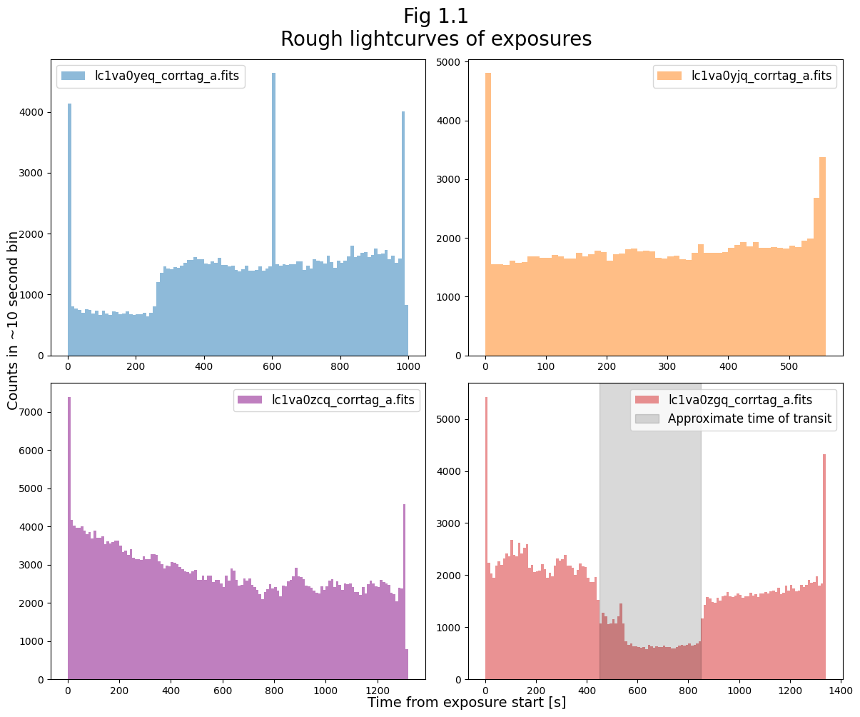
We can see an apparent transit in the exposure lc1va0zgq, occurring from about 450 - 850 seconds into the exposure. We highlight this in Figure 1.2 below.

Exposure lc1va0yeq also seems to contain at least the latter part of a transit, but for now we’ll focus on lc1va0zgq.

# Create the plot:
fig = plt.figure(figsize=(12, 6))

# Select the data and plot it:
# Binsize in seconds
binsize = 5
# Reading the corrtag table for this exposure
ctab = Table.read(transit_exp, 1)
# Getting the event times
event_times = ctab['TIME']
hist = plt.hist(event_times,
                bins=np.arange(0, max(event_times)+binsize, binsize),
                color='k',
                alpha=0.7)

# Add time ranges "epochs" or "windows of time" as transparent spans:
epoch_markers = [(0, 550), (550, 850), (850, max(event_times))]
print(f"The length of the exposure is ~{int(max(event_times))} s")
epoch_labels = ["Before Transit", "During Transit", "After Transit"]

# Adding color to distinguish before, during, and after the transit
for epoch_time, epoch_label, color in zip(epoch_markers, epoch_labels, ['b', 'orange', 'r']):
    plt.axvspan(
        epoch_time[0], epoch_time[1],
        color=color,
        alpha=0.2,
        label=epoch_label
    )

# Format the Figure
plt.legend(fontsize=12)

# Getting the transit file basename
transit_basename = transit_exp.split('/')[3]

plt.title(f"Fig 1.2\nRough lightcurves of exposure {transit_basename}",
          size=20)
plt.xlabel("Time from exposure start [s]",
           fontsize=14)
plt.ylabel(fr"Counts in ~{binsize} second bin",
           fontsize=14)

plt.tight_layout()

plt.savefig(plots_dir / 'examine_transit.png',
            bbox_inches='tight',
            dpi=200)

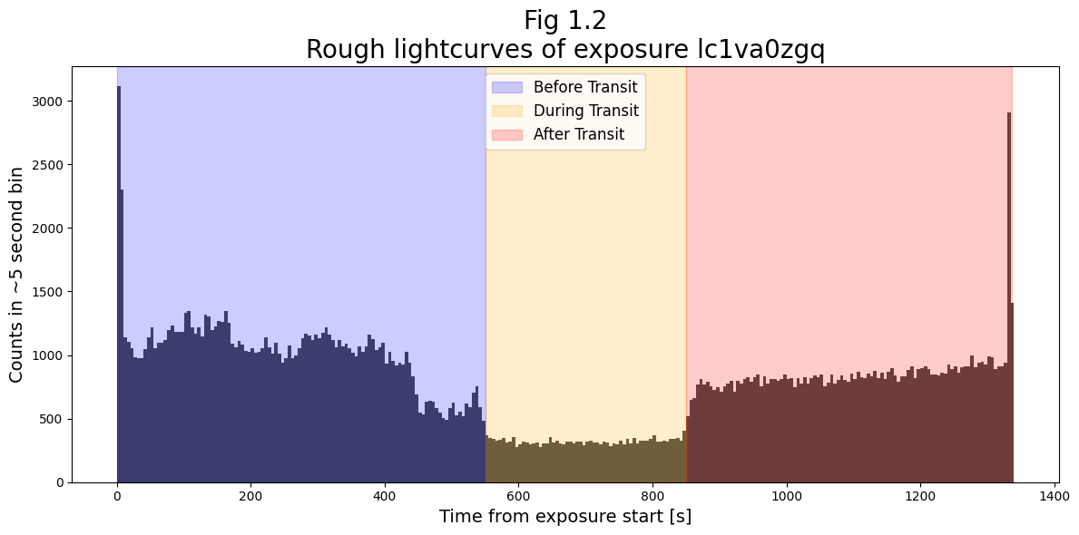
We now wish to actually split the file into three sub-exposures with the counts gathered during these three windows of time.

For research purposes, the transit should be measured more carefully than simply looking at this rough lightcurve. However for our purposes, we explicitly and somewhat arbitrarily define the windows, ‘by eye’, as:

Window	Time Range
Before Transit	0-550 seconds
During Transit	550-850 seconds
After Transit	850-1337 seconds

2. Using splittag to create multiple sub-exposure files

The next cell creates a directory for the sub-exposure files we’re about to create, and uses splittag to split the exposures.

The time_list parameter defines the times at which the exposure will be split. Because we pass this parameter the list [0, 550, 850, <time of last recorded count>], splittag will produce 3 sub-exposure files with data taken from:

1. 0-550 seconds

2. 550-850 seconds

3. 850-1337 seconds (because the <time of last recorded count> for this exposure ~1337 s)

Please note that splittag will not overwrite files if you run it multiple times. Instead, it will write a new set of files with increasing numeric suffixes (e.g. filepath_corrtag_a.fits –> filepath_1_corrtag_a.fits). This can cause issues if you do not update your filepaths to the output files you wish to use. To prevent problems, we will delete any older corrtag files in the directory. If you do not wish to delete your old files, set the delete_old_files variable to False in the cell below. Alternatively, you may wish to create a new directory for each time you run splittag. Please take care to prevent these issues when attempting the exercises, as well. You may ignore any AstropyDeprecationWarnings about keywords.

# Make the folder in which to store the newly split corrtag files:
spec_int_dir = output_dir / 'spec_intervals'
# An output directory for files split on specified intervals
spec_int_dir.mkdir(exist_ok=True)

# Use CAUTION when deleting files - as in the next lines:

# These lines delete existing processed files in the output directory
# If you have run this cell before, this will overwrite previous outputs
delete_old_files = True
if delete_old_files and any(spec_int_dir.glob("*corrtag*fits")):
    print("Deleting files from a previous run...")
    [old_f.unlink() for old_f in list(spec_int_dir.glob("*corrtag*fits"))]

# Print info to the user:
print("Creating and writing split files...")
for i, epoch_times in enumerate(epoch_markers):
    print(
        f"> File {i+1} contains counts from time:",
        f"{epoch_times[0]} - {epoch_times[1]} seconds"
    )

split_list = [0, 550, 850, max(event_times)]

# Run splittag using our specified times:
splittag.splittag(infiles=transit_exp,
                  outroot=f'./output/spec_intervals/{transit_basename}',
                  time_list=split_list)

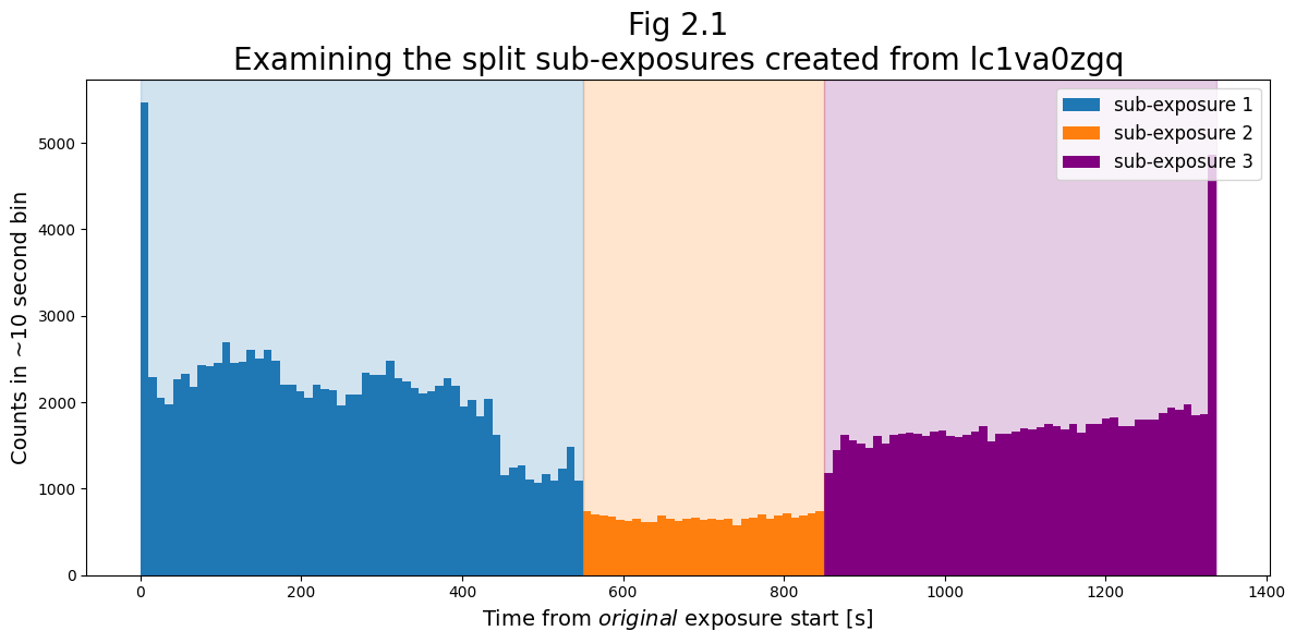
Excellent! We’ve now created 3 sub-exposure files.

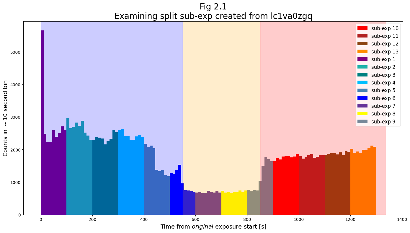
Below, we show the lightcurves of sub-exposure files which resulted from splitting at the specified intervals.

# Create the plot:
fig = plt.figure(figsize=(12, 6))

# Gather the split sub-exposure files:
spec_outlist = sorted(glob.glob('./output/spec_intervals/*fits'))

# Make histogram lightcurves as in previous plots:

# Binsize of lightcurve histogram in seconds
binsize = 10
# For each of our newly split up files:
for i in range(len(spec_outlist)):
    splitfile = spec_outlist[i]
    epoch_number = splitfile.split('_')[2]
    # Read in the file as a table of events:
    events_table = Table.read(splitfile, 1)
    event_times = events_table['TIME']
    hist = plt.hist(
        event_times,
        bins=int((max(event_times)-min(event_times))/binsize),
        alpha=1,
        color=['C0', 'C1', 'purple'][i],
        label=f"sub-exposure {epoch_number}"
    )

# Add time ranges "epochs" or "windows of time" as transparent spans:
for epoch_time, color in zip(epoch_markers, ['C0', 'C1', 'purple']):
    plt.axvspan(
        epoch_time[0], epoch_time[1],
        color=color,
        alpha=0.2,
        label=None
    )

# Format the Figure
plt.legend(fontsize=12)

plt.title("Fig 2.1\nExamining the split sub-exposures created "
          + f"from {transit_basename}",
          size=20)
plt.xlabel("Time from $original$ exposure start [s]",
           fontsize=14)
plt.ylabel(fr"Counts in ~{binsize} second bin",
           fontsize=14)

plt.tight_layout()

plt.savefig(plots_dir / 'subexps.png',
            bbox_inches='tight',
            dpi=200)

Now that we have the three sub-exposure files, we can process them into 1-dimensional spectra using the COS Calibration Pipeline: CalCOS.

Exercise 1: Practice sub-dividing with splittag

Examining Fig 2.1, we see that from approximately 450-550 seconds, there is are in fact 2 drops in flux. Starting from an initial flux similar to that at the start of the exposure, the flux drops first by ~50% at around 450 seconds, and then drops by ~75% at around 550 seconds to its depth for the duration of the transit.

Separate out the data taken during this initial drop (from ~450-550 seconds) into its own sub-exposure file using splittag. Then, demonstrate your split files with a lightcurve like that in Fig 2.1.

# Your code here:

3. Extracting spectra from the sub-exposures using CalCOS

While for most circumstances, CalCOS is best run on an association file, (a FITS table which specifies a series of exposures to calibrate and combine into a spectrum,) the CalCOS pipeline can usually be run on individual rawtag or corrtag files.

• More information on running CalCOS can be found in Chapter 3.6 of the COS Instrument Handbook

• An interactive walkthrough to running the CalCOS can be found in our notebook on the CalCOS pipeline.

3.1 Getting the lref reference files

To run CalCOS, your computer will need an lref system variable to tell the pipeline where to find your reference files. If you are on the STScI internet network (including via VPN), you may set this to the shared Institute lref directory. However, if you’re not on the network, you will need to use the CRDS command to download the necessary reference files. This process is described in detail in Chapter 3 of our notebook on setting up an environment for working with COS data.

The code in this cell ensures that the “lref” path is correctly set in the environment variables. If “lref” is not already defined, it will be defined and the crds files will be downloaded. If you have already downloaded the files, the CRDS cache on your computer will be used, as shown in the “else” block.

# Check if "lref" is not set in the environment variables
if not os.environ.get('lref'):
    # If on STScI Network/VPN
    if os.path.exists('/grp/hst/cdbs/lref/'):
        os.environ['lref'] = '/grp/hst/cdbs/lref/'
        print("It looks like you are on the STScI " +
              "network; setting lref to '/grp/hst/cdbs/lref/'")
    # If not on STScI Network/VPN
    else:
        if os.name == "nt":
            home_directory = os.environ["USERPROFILE"]
        home_directory = os.environ["HOME"]
        crds_path = os.path.join(home_directory, "crds_cache")
        os.environ["CRDS_PATH"] = crds_path
        # URL for the STScI CRDS page
        crds_server_url = "https://hst-crds.stsci.edu"
        # Setting env variable to URL
        os.environ["CRDS_SERVER_URL"] = crds_server_url
        # Synchronize CRDS and fetch references
        !crds sync --contexts hst_cos_0347.imap --fetch-references
        lref = os.path.join(crds_path, "references/hst/cos")
        os.environ['lref'] = lref
        # Check if that path exists
        if not os.path.exists(os.environ['lref']):
            print("It doesn't look like that's a valid path. Deleting it.")
            # delete this nonexistant path
            del os.environ['lref']
else:
    # Set home_directory
    # For windows:  
    if os.name == "nt":
        home_directory = os.environ["USERPROFILE"]
    # Other operating systems
    else:
        home_directory = os.path.expanduser("~")
    # Get the home directory from the lref
    lref = os.environ['lref']
    # Replace the {HOME} placeholder with the home directory path
    expanded_path = lref.replace("{HOME}", home_directory)
    os.environ['lref'] = expanded_path
    print(f"You already have an lref path in your env variables: {lref}\n")

assert os.path.exists(os.environ['lref']), "Path to lref directory " + \
                        "is invalid ({os.environ['lref']})"

3.2 Running CalCOS and processing sub-exposure files

We can now run the pipeline on each of our new sub-exposure files to create processed spectra based on data taken in the three time periods.

The cells may take several minutes to run.

# When we run CalCOS on corrtags, we must go 1-by-1
for split_corrtag in spec_outlist:
    # Define epoch as chunk of the initial exposure. epoch 2 = the transit.
    epoch_number = os.path.basename(split_corrtag).split('_')[1]
    print(f"Extracting file {split_corrtag} using CalCOS")

    # Make a sub-directory of output/calcos/ named for each epoch:
    cal_output_dir = f'./output/calcos/epoch{epoch_number}/'
    os.makedirs(cal_output_dir, exist_ok=True)

    # Extract the spectrum from each of the sub-exposures:
    try:
        calcos.calcos(split_corrtag,
                      outdir=cal_output_dir,
                      verbosity=0)
    except RuntimeError as e:
        print('An error occured', e)

# Print a message at the end to let us know it's finished:
print("Done running the pipeline.")

Now, we can examine our newly processed spectra

We first examine the entire spectrum:

# Find all the `x1d` files:
processed_files = sorted(glob.glob('output/calcos/epoch*/*x1d.fits'))

# Set up figure
plt.figure(figsize=(18, 12))

# Loop through
for i in range(len(processed_files)):
    epoch_label = processed_files[i].split('/')[2]

    # Mark the transit
    if "2" in epoch_label:
        epoch_label += " (transit)"

    with warnings.catch_warnings():
        warnings.filterwarnings('ignore',
                                category=UnitsWarning,
                                append=True)

        w, f, ferr, dq = Table.read(
            processed_files[i])[0]['WAVELENGTH', 'FLUX', 'ERROR', 'DQ']

    # Filter to good quality data
    dq_mask = np.where(dq == 0)
    w, f, ferr = w[dq_mask], f[dq_mask], ferr[dq_mask]

    # Plot each epoch
    plt.plot(w, f,
             # Epoch2 should stand out
             alpha=[0.5, 1, 0.5][i],
             c=['b', 'purple', 'r'][i],
             # Label with the epoch name
             label=epoch_label)

# Format plot
plt.ylim(-3E-15, 5E-14)

plt.title("Fig 3.1\nComparison of processed spectra",
          size=22)
plt.xlabel(r"Wavelength [$\AA$]",
           size=14)
plt.ylabel(r"Flux [$ergs\ cm^{-2} \AA^{-1}s^{-1}$]",
           size=14)

plt.legend()

plt.savefig(plots_dir / "Compare_spectrum.png",
            dpi=200)

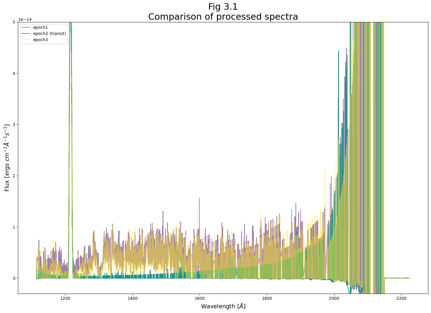
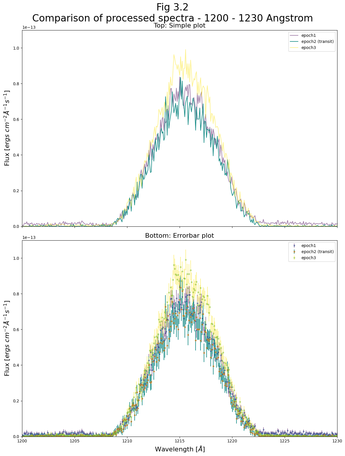
Now we can take a closer look at two spectral regions the region from 1200 - 1230 and from 1250 - 1350 Angstroms. In the first region, we see the 1215 Angstrom Lyman-alpha line, much of which is generated by geocoronal emission. At this line, the flux of the the three epochs is very similar, because the transit in the IY UMa system has no effect on Earth’s atmosphere. There are slight differences because the sun’s changing position in the sky changes the geocoronal glow. This causes the third sub-exposure to have a slightly higher Lyman-alpha line. However these are small differences compared to the flux of these lines.

For this and the following plots, we will plot the errors as well, to see if the apparent differences in flux between epochs are significant.

For the 1200 - 1230 Angstrom region:

# Set up figure
fig, (ax0, ax1) = plt.subplots(2, 1,
                               figsize=(12, 16),
                               sharex=True)

for i in range(len(processed_files)):
    epoch_label = processed_files[i].split('/')[2]
    if "2" in epoch_label:
        epoch_label += " (transit)"

    with warnings.catch_warnings():
        warnings.filterwarnings('ignore',
                                category=UnitsWarning,
                                append=True)

        w, f, ferr, dq = Table.read(
            processed_files[i])[0]['WAVELENGTH', 'FLUX', 'ERROR', 'DQ']

    # Filter to good quality data
    dq_mask = np.where(dq == 0)
    w, f, ferr = w[dq_mask], f[dq_mask], ferr[dq_mask]

    # Plot each epoch
    ax0.plot(w, f,
             # Epoch2 should stand out
             alpha=[0.5, 1, 0.5][i],
             c=['b', 'purple', 'r'][i],
             linestyle='-',
             # Label with the epoch name
             label=epoch_label)

    # Plot each epoch
    ax1.errorbar(w, f, yerr=ferr,
                 # Epoch2 should stand out
                 alpha=[0.5, 1, 0.5][i],
                 marker='.',
                 markerfacecolor=['b', 'purple', 'r'][i],
                 linestyle='',
                 ecolor=['b', 'purple', 'r'][i],
                 # Label with the epoch name
                 label=epoch_label)

# Format both subplots
ax0.set_xlim(1200, 1230)
ax0.set_ylim(0, 1.1E-13)
ax1.set_ylim(0, 1.1E-13)

ax0.set_title("Top: Simple plot",
              fontsize=16)
ax1.set_title("Bottom: Errorbar plot",
              fontsize=16)
plt.suptitle(
    "Fig 3.2\nComparison of processed spectra - 1200 - 1230 Angstrom",
    size=24
)

ax1.set_xlabel(r"Wavelength [$\AA$]",
               size=16)
ax0.set_ylabel(r"Flux [$ergs\ cm^{-2} \AA^{-1}s^{-1}$]",
               size=16)
ax1.set_ylabel(r"Flux [$ergs\ cm^{-2} \AA^{-1}s^{-1}$]",
               size=16)

ax0.legend()
ax1.legend()

plt.tight_layout()

plt.savefig(plots_dir / "Compare_spectrum_zoom_1215A.png",
            dpi=200)

For the 1250 - 1350 Angstrom region:

# Set up figure
fig, (ax0, ax1) = plt.subplots(2, 1,
                               figsize=(12, 16),
                               sharex=True)

for i in range(len(processed_files)):
    epoch_label = processed_files[i].split('/')[2]
    if "2" in epoch_label:
        epoch_label += " (transit)"

    with warnings.catch_warnings():
        warnings.filterwarnings('ignore',
                                category=UnitsWarning,
                                append=True)

        w, f, ferr, dq = Table.read(
            processed_files[i])[0]['WAVELENGTH', 'FLUX', 'ERROR', 'DQ']

    # Filter to good quality data
    dq_mask = np.where(dq == 0)
    w, f, ferr = w[dq_mask], f[dq_mask], ferr[dq_mask]

    # Plot each epoch
    ax0.plot(w, f,
             # Epoch2 should stand out
             alpha=[0.5, 1, 0.5][i],
             c=['b', 'purple', 'r'][i],
             linestyle='-',
             # Label with the epoch name
             label=epoch_label)

    # Plot each epoch
    ax1.errorbar(w, f, yerr=ferr,
                 # Epoch2 should stand out
                 alpha=[0.5, 1, 0.5][i],
                 marker='.',
                 markerfacecolor=['b', 'purple', 'r'][i],
                 linestyle='',
                 ecolor=['b', 'purple', 'r'][i],
                 # Label with the epoch name
                 label=epoch_label)

# Format both subplots:
# Zoom to 1250-1350 Angstrom
ax0.set_xlim(1250, 1350)
ax1.set_xlim(1250, 1350)

ax0.set_ylim(-5.E-16, 1.1E-14)
ax1.set_ylim(-5.E-16, 1.1E-14)

ax0.set_title("Top: Simple plot",
              fontsize=16)
ax1.set_title("Bottom: Errorbar plot",
              fontsize=16)

plt.suptitle(
    "Fig 3.3\nComparison of processed spectra - 1250 - 1350 Angstrom",
    size=24
)

ax1.set_xlabel(r"Wavelength [$\AA$]",
               size=16)
ax0.set_ylabel(r"Flux [$ergs\ cm^{-2} \AA^{-1}s^{-1}$]",
               size=16)
ax1.set_ylabel(r"Flux [$ergs\ cm^{-2} \AA^{-1}s^{-1}$]",
               size=16)

ax0.legend()
ax1.legend()

plt.tight_layout()

plt.savefig(plots_dir / "Compare_spectrum_zoom.png",
            dpi=200)

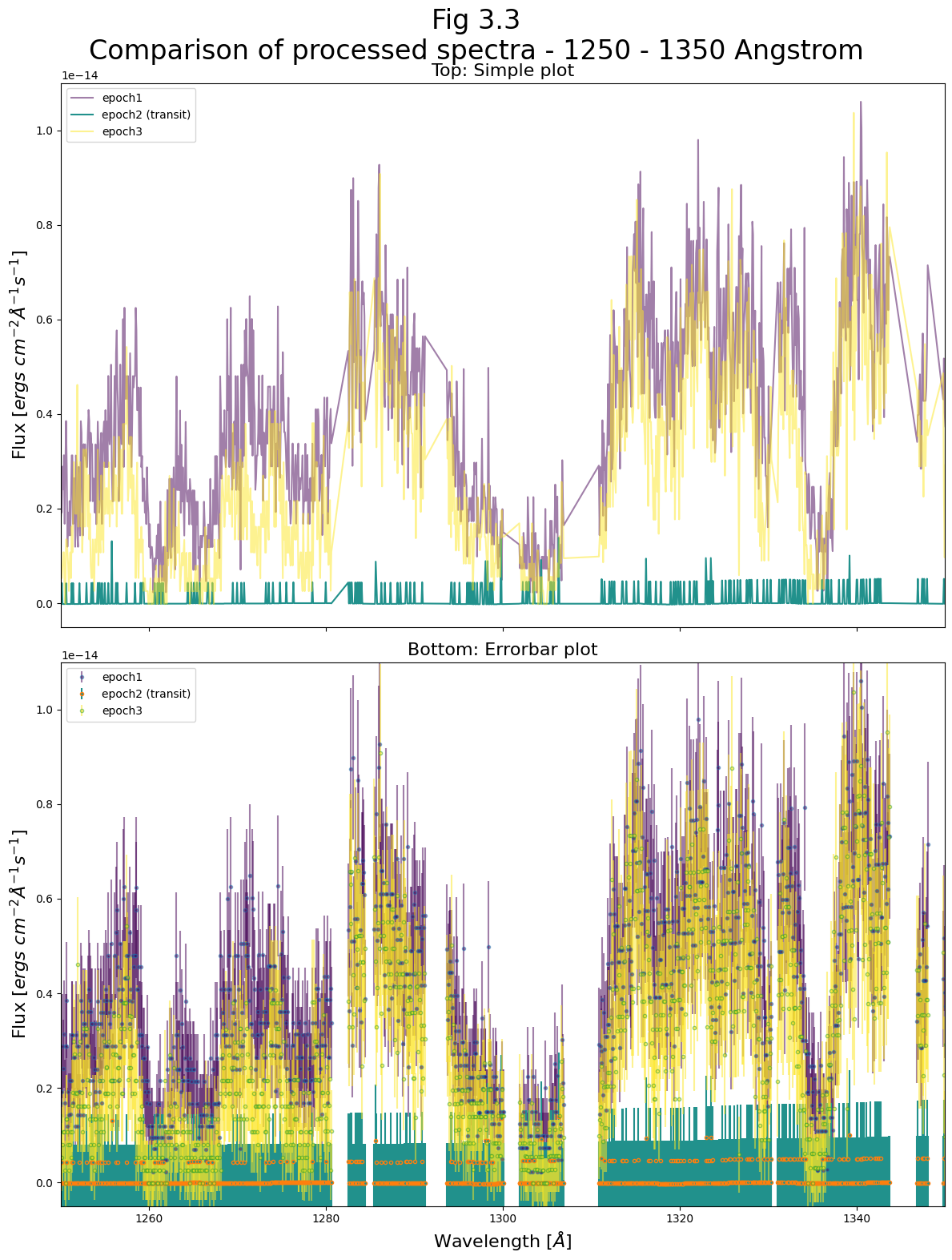
Examining Fig 3.3, we first notice that the very low number of counts in a given wavelength region has limited our spectra’s precision. This is especially evidenced by how epoch 2’s flux is visibly quantized to several values, corresponding with the very low numbers of counted photons in each wavelength bin.

However, we can still detect a significant change in the spectrum during the transit, with certain spectral features absent or suppressed while the transit occurs. During the transit, COS receives almost no photons coming from the source at these spectral features.

4. Creating multiple sub-exposure files at regular intervals

Above, we split an input exposure at a series of specified times. The splittag command can also be used to split at regular time intervals. For instance, you can split the file every 100 seconds as shown in the code below:

# Make the folder in which to store the newly split corrtag files:
reg_int_dir = output_dir / 'regular_intervals'
# Output directory for intervals specified by start/end/length
reg_int_dir.mkdir(exist_ok=True)

# Split the file every 100 seconds
if not any(reg_int_dir.iterdir()):
    splittag.splittag(
        infiles=transit_exp,
        outroot='./output/regular_intervals/lc1va0zgq',
        starttime=0,
        increment=100,
        endtime=1300.
    )
print("files already exist")

Similarly to our 3 epoch sub-exposures, we can show the light curve of our 100s regularly spaced sub-exposure files:

# Creating an array of colors for this exposure to be used in plotting
colors = [
    'red',
    'firebrick',
    'saddlebrown',
    'darkorange',
    'purple',
    'lightseagreen',
    'teal',
    'deepskyblue',
    'steelblue',
    'blue',
    'rebeccapurple',
    'yellow',
    'lightslategrey'
]

# Create the plot:
fig = plt.figure(figsize=(14, 8))

# Gather the split sub-exposure files:
spec_outlist = sorted(glob.glob('./output/regular_intervals/*fits'))

# Make histogram lightcurves as in previous plots:
# Binsize of lightcurve histogram in seconds
binsize = 10

# For each of our newly split up files:
for i in range(len(spec_outlist)):
    splitfile = spec_outlist[i]
    epoch_number = splitfile.split('_')[2]

    # Read in the file as a table of events:
    events_table = Table.read(splitfile, 1)
    event_times = events_table['TIME']

    hist = plt.hist(
        event_times,
        bins=int((max(event_times)-min(event_times))/binsize),
        alpha=1,
        color=colors[i],
        label=f"sub-exp {epoch_number}"
    )

# Add time ranges "epochs" or "windows of time" as transparent spans:
for epoch_time, color in zip(epoch_markers, ['b', 'orange', 'r']):
    plt.axvspan(
        epoch_time[0], epoch_time[1],
        color=color,
        alpha=0.2,
        label=None
    )

# Format the Figure
plt.legend(fontsize=12)

plt.title(f"Fig 2.1\nExamining split sub-exp created from {transit_basename}",
          size=20)
plt.xlabel("Time from $original$ exposure start [s]",
           fontsize=14)
plt.ylabel(fr"Counts in $\sim${binsize} second bin",
           fontsize=14)

plt.tight_layout()

plt.savefig(plots_dir / 'subexps.png',
            bbox_inches='tight',
            dpi=200)

Exercise 2: Examining epoch 1.5

From Exercise 1, you have an additional epoch, from 450-550 seconds, which overlaps with the end of epoch 1, and has a flux between epoch 1 and epoch 2.

We wish to know whether the data taken during epoch 1.5 more closely aligns with that during epoch 1 or 2. To analyze this,

• 2.1: Run epoch 1.5’s data through CalCOS

• 2.2: Plot epoch 1.5 alongside epochs 1 and 2 in the wavelength range around 1275 Å (i.e. recreate Fig. 3.2 without epoch 3 and with epoch 1.5).

• 2.3: Briefly analyze whether epoch 1.5 is more in line with epoch 1 or 2, and consider how this knowledge may be useful. Consider whether our approach here to answering this question has any major flaws.

# Your code here:

This is certainly not an exhaustive analysis, and we do not claim in this Notebook to have made any measurements confirming or quantifying a transit.

However, you should now be equipped to use the splittag tool to subdivide exposures to look for time-variable phenomena.

Congratulations! You finished this Notebook!

There are more COS data walkthrough Notebooks on different topics. You can find them here.

---

About this Notebook

Author: Nat Kerman: nkerman@stsci.edu

Contributors: This Notebook drew from a previously existing Notebook written by Justin Ely.

Updated On: 2022-01-04

This tutorial was generated to be in compliance with the STScI style guides and would like to cite the Jupyter guide in particular.

Citations

If you use astropy, matplotlib, astroquery, or numpy for published research, please cite the authors. Follow these links for more information about citations:

• Citing numpy

• Citing astropy

• Citing matplotlib

• Citing astroquery

---

Top of Page

Exercise Solutions

# Exercise 1:

# Make the folder in which to store the newly split corrtag files:
spec_int_dir2 = output_dir / 'spec_intervals_Ex1'
# A second output directory for files split on specified intervals
spec_int_dir2.mkdir(exist_ok=True)

# List the specified times
split_list = [0, 450, 550, 1337]

# Run splittag using our specified times:
splittag.splittag(infiles=transit_exp,
                  outroot=spec_int_dir2 / 'transit_basename',
                  time_list=split_list)

# Exercise 2.1 (CalCOS):

# Make a sub-directory of output/calcos/examples named for this epoch.
# We'll call the epoch "1.5" because it's between epochs 1 and 2
calcos_dir = Path('./output/calcos') 
examples_dir = calcos_dir / 'examples'
epoch_dir = examples_dir / 'epoch1.5'

calcos_dir.mkdir(exist_ok=True)
examples_dir.mkdir(exist_ok=True)
epoch_dir.mkdir(exist_ok=True)

# Extract the spectrum from the 2nd sub-exposure in spec_intervals_Ex1:
try:
    calcos.calcos(
        'output/spec_intervals_Ex1/transit_basename_2_corrtag_a.fits',
        outdir=epoch_dir,
        verbosity=0
    )
except RuntimeError as e:
    print('An error occured', e)

# Exercise 2.2 (Plotting):

# Set up figure
fig, (ax0, ax1) = plt.subplots(2, 1,
                               figsize=(12, 16),
                               sharex=True)

# Specify the files explicitly here
processed_example_files = [
    'output/calcos/epoch1/lc1va0zgq_1_x1d.fits',
    'output/calcos/examples/epoch1.5/transit_basename_2_x1d.fits',
    'output/calcos/epoch2/lc1va0zgq_2_x1d.fits',
]

for i in range(len(processed_example_files)):
    epoch_label = processed_example_files[i].split('/')[2]

    with warnings.catch_warnings():
        warnings.filterwarnings('ignore',
                                category=UnitsWarning,
                                append=True)

        w, f, ferr, dq = Table.read(
            processed_example_files[i])[0]['WAVELENGTH', 'FLUX', 'ERROR', 'DQ']

    # Filter to good quality data
    dq_mask = np.where(dq == 0)
    w, f, ferr = w[dq_mask], f[dq_mask], ferr[dq_mask]

    # Plot each epoch
    ax0.scatter(w, f,
                # Epoch 2 should stand out
                alpha=[0.5, 1, 0.5][i],
                c=['C0', 'k', 'c'][i],
                linestyle='-',
                # Label with the epoch name
                label=epoch_label)

    # Plot each epoch
    ax1.errorbar(w, f, yerr=ferr,
                 # Epoch 2 should stand out
                 alpha=[0.5, 1, 0.5][i],
                 marker='.',
                 markerfacecolor=['C0', 'r', 'c'][i],
                 linestyle='',
                 ecolor=['C0', 'k', 'c'][i],
                 # Label with the epoch name
                 label=epoch_label)

# Format both subplots
# Zoom to 1225 - 1300 Angstrom
ax0.set_xlim(1250, 1300)
ax1.set_xlim(1250, 1300)
ax0.set_ylim(-5.E-16, 1.1E-14)
ax1.set_ylim(-5.E-16, 1.1E-14)

ax0.set_title("Top: Simple plot",
              fontsize=16)
ax1.set_title("Bottom: Errorbar plot",
              fontsize=16)
plt.suptitle(
    "Fig Ex2.1\nComparison of processed spectra - Zoom on source spectrum",
    size=24
)

ax1.set_xlabel(r"Wavelength [$\AA$]",
               size=16)
ax0.set_ylabel(r"Flux [$ergs\ cm^{-2} \AA^{-1}s^{-1}$]",
               size=16)
ax1.set_ylabel(r"Flux [$ergs\ cm^{-2} \AA^{-1}s^{-1}$]",
               size=16)

ax0.legend()
ax1.legend()

plt.tight_layout()

plt.savefig(
    plots_dir / "Compare_spectrum_zoom_1275A_Ex2.png",
    dpi=200
)

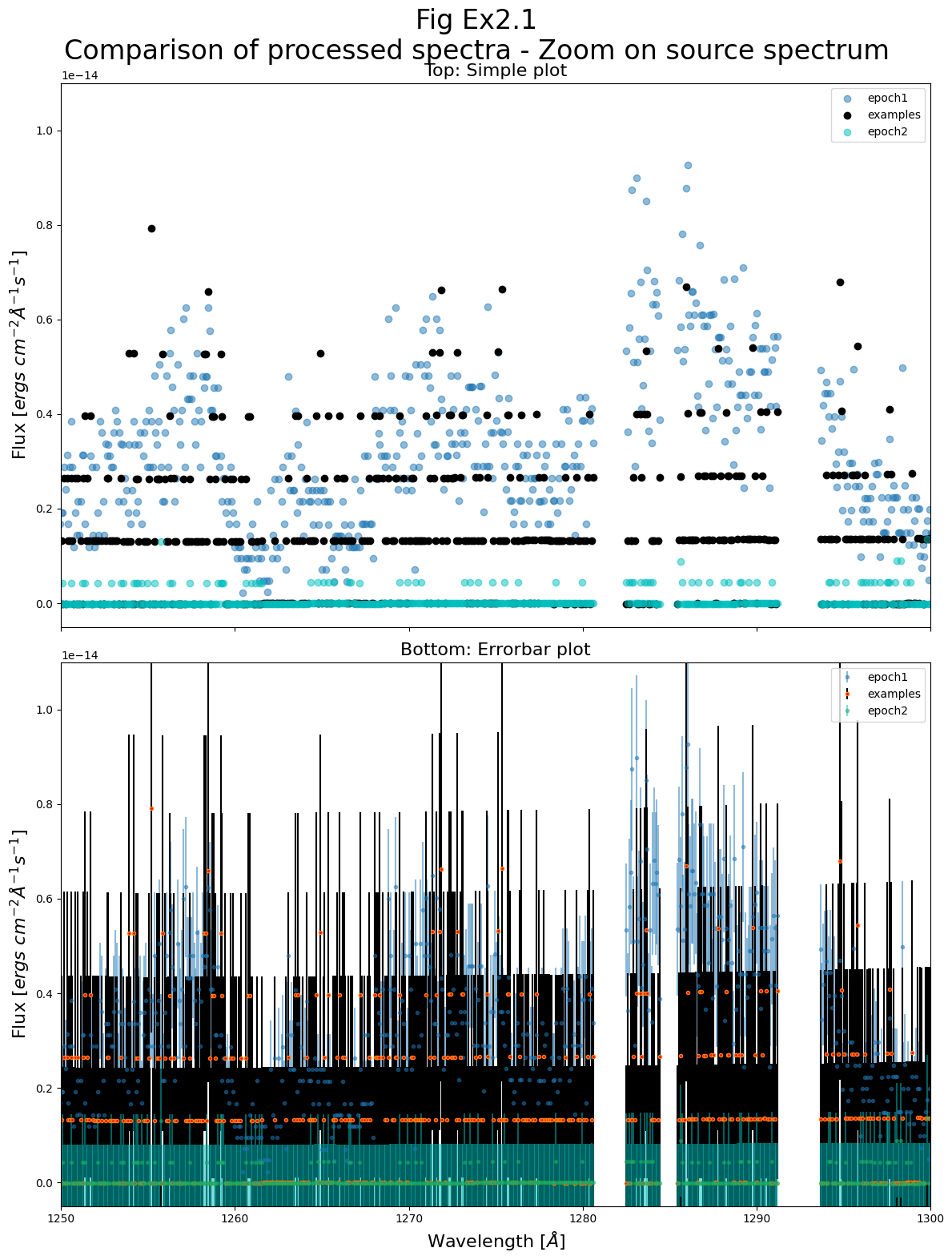
Ex 2.3 (Analysis):

From a brief look, it seems that epoch 1.5 shares much more in common with epoch 1 (before the transit) than epoch 2 (during the transit).

If we wished to get as good a signal to noise ratio observation of the pre-transit spectrum as possible, we might include epochs 1 and 1.5 together to get additional counts.

Note that epoch 1 contains all the counts from epoch 1.5, while epoch 2 does not. Thus this is not a perfect test. However, the vast majority of epoch 1’s counts do not overlap with epoch 1.5 (see fig 2.1), so this is an acceptable “first pass” test. It’s also possible that the very low number of counts, especially in epochs 1.5 and 2, does not give us the signal-to-noise we would need to accurately distinguish the epochs.