Custom CCD Darks

Custom CCD Darks #

This notebook currently fails to execute, use as reference only

Learning Goals

1 Introduction
- 1.1 Import Necessary Packages
- 1.2 Collect Data Set From the MAST Archive Using Astroquery
2 Default Dark File
3 Make Basedark
4 Make Weekdark
5 Calibrate with New Weekdark
- 5.1 Calibration
- 5.2 Comparison With the Default Dark File

Introduction#

In the Calstis pipline for calibrating STIS CCD data, one of the steps is dark signal substraction, which removes the dark signal (count rate created in the detector in the absence of photons from the sky) from the uncalibrated science image based on reference file. Usually, the Calstis pipline uses the default dark reference file specified in the 0-extension header of the uncalibrated science image fits file. But for some faint sources, it is necessary to customize the dark reference for the observations to remove the hot pixels in the science image. In this notebook, we will go through how to create dark reference files using the Python refstis library.

Notice: this notebook demonstrates a squence of steps to customize dark reference file. If any of the intermediate steps fail or need to rerun, please restart the ipython kernel and start from the first step.

Import Necessary Packages#

astropy.io fits astropy.table for accessing FITS files
astroquery.mast Observations for finding and downloading data from the MAST archive
os,shutil,pathlib for managing system paths
numpy to handle array functions
stistools for calibrating STIS data
refstis for creating STIS reference files
matplotlib for plotting data

For more information on installing refstis, see: Refstis: Superdarks and Superbiases for STIS

# Import for: Reading in fits file
from astropy.io import fits
from astropy.table import Table

# Import for: Downloading necessary files. (Not necessary if you choose to collect data from MAST)
from astroquery.mast import Observations

# Import for: Managing system variables and paths
import os
import shutil
from pathlib import Path

# Import for: Quick Calculation and Data Analysis
import numpy as np

# Import for: Operations on STIS Data
import stistools
from refstis.basedark import make_basedark
from refstis.weekdark import make_weekdark

# Import for: Plotting and specifying plotting parameters
import matplotlib
%matplotlib inline
from matplotlib import pyplot as plt

matplotlib.rcParams['image.origin'] = 'lower'
matplotlib.rcParams['image.cmap'] = 'plasma'
matplotlib.rcParams['image.interpolation'] = 'none'
matplotlib.rcParams['figure.figsize'] = (20, 10)

Collect Data Set From the MAST Archive Using Astroquery#

There are other ways to download data from MAST such as using CyberDuck. The steps of collecting data is beyond the scope of this notebook, and we are only showing how to use astroquery and CRDS.

%%capture --no-display
# cleanup download directory
if os.path.exists('./mastDownload'):
    shutil.rmtree('./mastDownload')

# change this field in you have a specific dataset to be explored
obs_id = "oeik1s030"
# Search target by obs_id
target = Observations.query_criteria(obs_id=obs_id)
# get a list of files assiciated with that target
FUV_list = Observations.get_product_list(target)
# Download fits files
result = Observations.download_products(FUV_list, extension='fits')
crj = os.path.join("./mastDownload/HST", "{}".format(obs_id), "{}_crj.fits".format(obs_id))

Next, use the Calibration Reference Data System (CRDS) command line tools to update and download the reference files for creating the basedark.

crds_path = os.path.expanduser("~") + "/crds_cache"
os.environ["CRDS_PATH"] = crds_path
os.environ["CRDS_SERVER_URL"] = "https://hst-crds.stsci.edu"
os.environ["oref"] = os.path.join(crds_path, "references/hst/oref/")

!crds bestrefs --update-bestrefs --sync-references=1 --files ./mastDownload/HST/oeik1s030/oeik1s030_raw.fits

Default Dark File#

The default dark file is specified in the 0th extension of an uncalibrated science image through a field called ‘DARKFILE’. We will later replace this default dark file with the customized dark file we created using refstis.

darkfile = fits.getval(crj, ext=0, keyword='DARKFILE')
print("The default dark file of observation {id} is: {df}".format(id=obs_id, df=darkfile))

Make Basedark#

Every month, a high signal-to-noise superdark frame is created from a combination of typically 40-60 “long” darks. These monthly superdark frames are not actually delivered to the calibration data base, but used as “baseline” dark for the next steps. When creating the Basedark, the input imsets are joined and combined into a single file, and the cosmic ray rejection is performed. Then the hot pixels in the combined image frame are identified and labeled in the DQ array using an iterative sigma clip method, and those hot pixels will later be updated with values in the Weekdark. In this section, we’ll show how to create the basedark file.

These superdark frames are not taken exactly each month, but during a roughly 30 days period called “annealing period”. The duration of each annealing period, together with the superdark frames taken, can be found here: STIS Annealing Periods.

We first get the observation date of our sample data, and find the corresponding anneal period:

TDATEOBS = fits.getval(crj, ext=0, keyword='TDATEOBS')
TTIMEOBS = fits.getval(crj, ext=0, keyword='TTIMEOBS')
print("UT date of start of first exposure in file is {}".format(TDATEOBS))
print("UT time of start of first exposure in file is {}".format(TTIMEOBS))

According to the STIS Annealing Periods, this observation was taken during the annealing period from 2021-04-07 02:35:41 to 2021-05-05 14:00:22. We collect all the long component dark flt data during that annealing period:

%%capture --no-display
# copy the dark file obs_id from the STIS Annealing Periods table, and put them into a list
rootnames = "oeen8lqwq, oeen8ms5q, oeen8nvcq, oeen8oxnq, oeen8pa3q, oeen8qckq, oeen8reyq, oeen8sguq, "\
            "oeen8taaq, oeen8udiq, oeen8vh3q, oeen8wicq, oeen8xkaq, oeen8yn4q, oeen8zpyq, oeen90rtq, oeen91u0q, oeen92wdq, "\
            "oeen93ysq, oeen94arq, oeen95dlq, oeen96g4q, oeen97b7q, oeen98c4q, oeen99gxq, oeen9ah3q, oeen9bm7q, oeen9cmkq, "\
            "oeen9dryq, oeen9et6q, oeen9fxwq, oeen9gy4q, oeen9icqq, oeen9hcwq, oeen9jgwq, oeen9kh4q, oeen9lafq, oeen9majq, "\
            "oeen9nh9q, oeen9ohiq, oeen9qovq, oeen9ppcq, oeen9rucq, oeen9supq, oeen9tydq, oeen9uytq, oeen9velq, oeen9wf3q, "\
            "oeen9xjeq, oeen9yjmq, oeen9za2q, oeena0aaq, oeena1g5q, oeena2gcq, oeena3kjq, oeena4knq".split(', ')
# search in astroquery based on obs_id
search = Observations.query_criteria(obs_id=rootnames)
pl = Observations.get_product_list(search)
# we only need the _flt fits files
pl = pl[pl['productSubGroupDescription'] == 'FLT']
# download the data
download_status = Observations.download_products(pl, mrp_only=False)
# store all the paths to the superdark frames into a list
anneal_dark = []
for root in rootnames:
    file_path = os.path.join("./mastDownload/HST", "{}".format(root), "{}_flt.fits".format(root))
    # check CCD amplifier
    CCDAMP = fits.getval(file_path, keyword='CCDAMP', ext=0)
    assert (CCDAMP == 'D')
    anneal_dark.append(file_path)

filename_mapping = {os.path.basename(x).rsplit('_', 1)[0]: x for x in download_status['Local Path']}

Then we put the list of input dark files into refstis.make_basedark. The second parameter, refdark_name, is the name of the output basedark file. For detailed information on make_basedark, see: Basedark.

new_basedark = 'new_basedark.fits'
# remove the new_basefark file if it already exists
if os.path.exists(new_basedark):
    os.remove(new_basedark)
make_basedark(anneal_dark, refdark_name=new_basedark, bias_file=None)

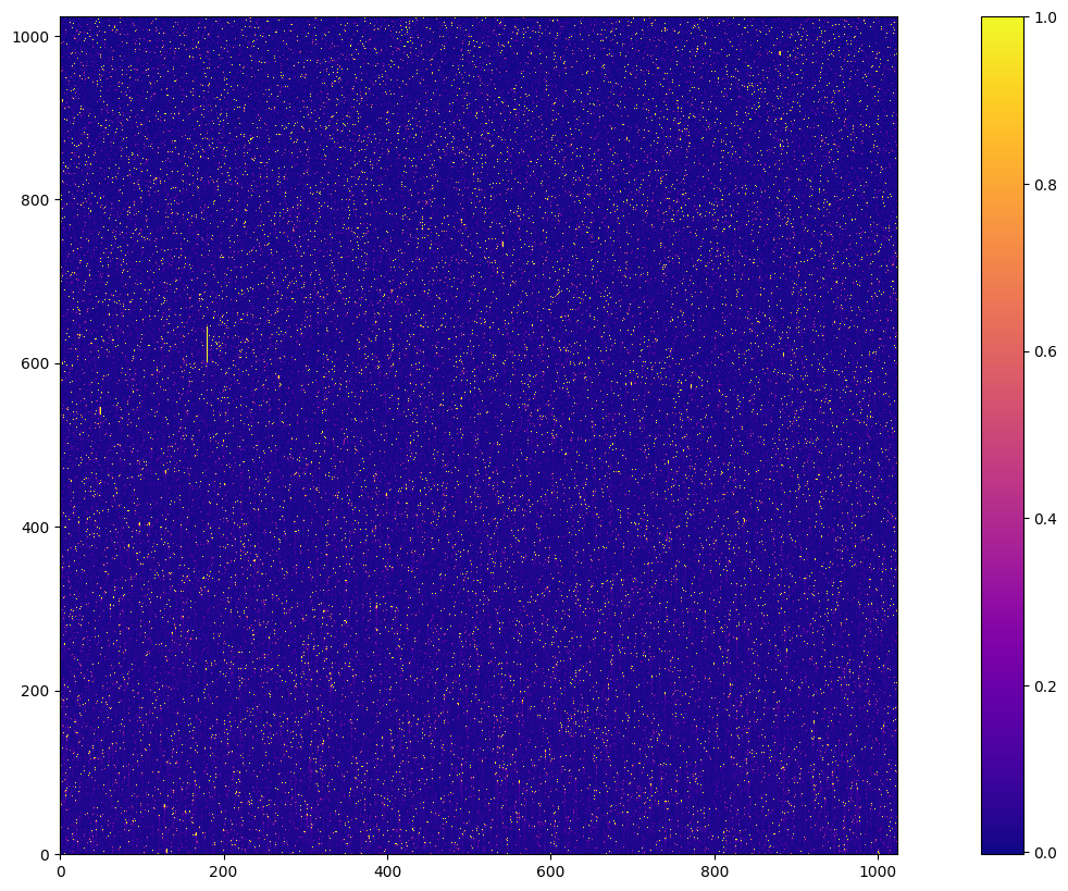
with fits.open(new_basedark) as hdu:
    new_basedark_data = hdu[1].data
cb = plt.imshow(new_basedark_data, cmap='plasma', vmax=1)
plt.colorbar(cb)

Make Weekdark#

The Weekdark is the combination of all “long” dark files from the week of the science observation, which is eventually passed into the Calstis pipline as the DARKFILE for the DARKCORR calibration. After the darks during a given week is combined and normalized to produce a weekly superdark, those hotpixels in the monthly Basedark are replaced by those of the normalized weekly superdark. The resulting dark has the high signal-to-noise ratio of the monthly baseline superdark, updated with the hot pixels of the current week.

We first search for the darks taken during the given week. We take the weekly period as the observation date ± 3 days in this demonstration, but notice here that since the observation time is 2021-05-05 12:29:54 while the ending time of the annealing period is 2021-05-05 14:00:22, observation date + 3 days will cross the annealing boundary. Therefore, in our case, we only take the observation date - 3 days as the weekly period. When you work with your own dataset, pay attention to the week boundary and annealing boundary to see if they completely overlap.

# search for darks taken during the weekly period (observation date, observation date + 3 days)
hdr = fits.getheader(crj, 0)
component_darks = Observations.query_criteria(
    target_name='DARK',
    t_min=[hdr['TEXPSTRT']-3, hdr['TEXPSTRT']],
    t_exptime=[1099, 1101])
# get a list of files assiciated with that target
dark_list = Observations.get_product_list(component_darks)
dark_list = dark_list[dark_list['productSubGroupDescription'] == 'FLT']
# store all the paths to the superdark frames into a list
component_flt = [filename_mapping[x] for x in component_darks['obs_id']]
component_flt

Now we have all the dark files we need to create the new weekdark reference file. Pass the list of the weekly component darks as the first parameter, the name of the new weekdark file as the second parameter, and the new basedark file we created above as the third parameter into refstis.make_weekdark. For more information on make_weekdark, see: Weekdark.

new_weekdark = "new_weekdark.fits"
# remove the new_basedark file if it already exists
if os.path.exists(new_weekdark):
    os.remove(new_weekdark)
make_weekdark(component_flt, new_weekdark, thebasedark=new_basedark)

Calibrate with New Weekdark#

Calibration#

Now we have created the new weekdark reference file for our specific dataset, we can use it to calibrate the raw data using Calstis. To change the dark reference file, we first set the value of DARKFILE in the _raw data 0th header using fits.setval. Calstis will then look for the DARKFILE value and use it as the reference file for DARKCORR.

raw = os.path.join("./mastDownload/HST", "{}".format(obs_id), "{}_raw.fits".format(obs_id))
wav = os.path.join("./mastDownload/HST", "{}".format(obs_id), "{}_wav.fits".format(obs_id))

# set the value of DARKFILE to the filename of the new week dark
fits.setval(raw, ext=0, keyword='DARKFILE', value=new_weekdark)
# make sure that the value is set correctly
fits.getval(raw, ext=0, keyword='DARKFILE')

Calibrate the _raw data using the new weekdark reference file:

# create a new folder to store the calibrated data
if os.path.exists('./new_dark'):
    shutil.rmtree('./new_dark')
Path('./new_dark').mkdir(exist_ok=True)
res = stistools.calstis.calstis(raw, wavecal=wav, outroot="./new_dark/")
assert res == 0, 'CalSTIS returned an error!'

with fits.open('new_weekdark.fits') as hdu:
    new_weekdark_data = hdu[1].data
cb = plt.imshow(new_weekdark_data, cmap='plasma', vmax=1)
plt.colorbar(cb)

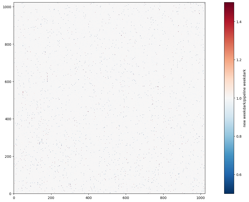
To compare the new weekdark science image with the old weekdark science image, we divide the new weekdark science image frame by that of the old weekdark, and use a diverging colormap to visulize the ratio. The colormap is normalized to center at 1, and the red pixels suggests that the ratio is greater than 1 while the blue pixels suggests that the ratio is less than 1. In general there are more blue pixels in the image, which means we are removing more hot pixels compared with the old weekdark.

with fits.open("55a20445o_drk.fits") as hdu:
    old_weekdark_data = hdu[1].data
cb = plt.imshow(new_weekdark_data/old_weekdark_data, cmap='RdBu_r', vmin=0.5, vmax=1.5)
plt.colorbar(cb, label="new weekdark/pipeline weekdark")

Comparison With the Default Dark File#

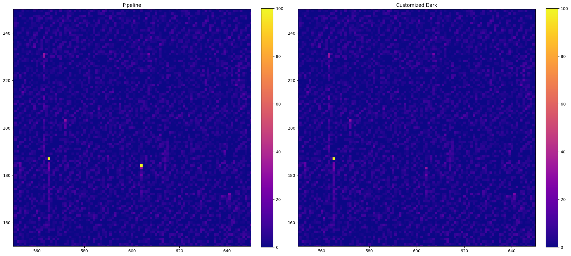
When we collected the science data from MAST, the _crj and _sx1 data files are already calibrated using the default dark reference file. We can make a comparison between the calibrated images and spectra of the defualt dark file and our new Weekdark. As shown in the comparison, a hot pixel is removed from the _crj image at x \(\approx\) 605 and y \(\approx\) 185.

# Plot the calibrated _crj images
# The left panel is the defalt _crj image from the pipline
# the right panel is calibrated with our customized dark file
plt.subplot(1, 2, 1)
with fits.open(crj) as hdu:
    ex1 = hdu[1].data
    cb = plt.imshow(ex1, vmin=0, vmax=100)
    plt.colorbar(cb, fraction=0.046, pad=0.04)
    plt.xlim(550, 650)
    plt.ylim(150, 250)
    plt.title("Pipeline")
plt.subplot(1, 2, 2)
with fits.open("./new_dark/oeik1s030_crj.fits") as hdu:
    ex1 = hdu[1].data
    cb = plt.imshow(ex1, vmin=0, vmax=100)
    plt.colorbar(cb, fraction=0.046, pad=0.04)
    plt.xlim(550, 650)
    plt.ylim(150, 250)
    plt.title("Customized Dark")
plt.tight_layout()

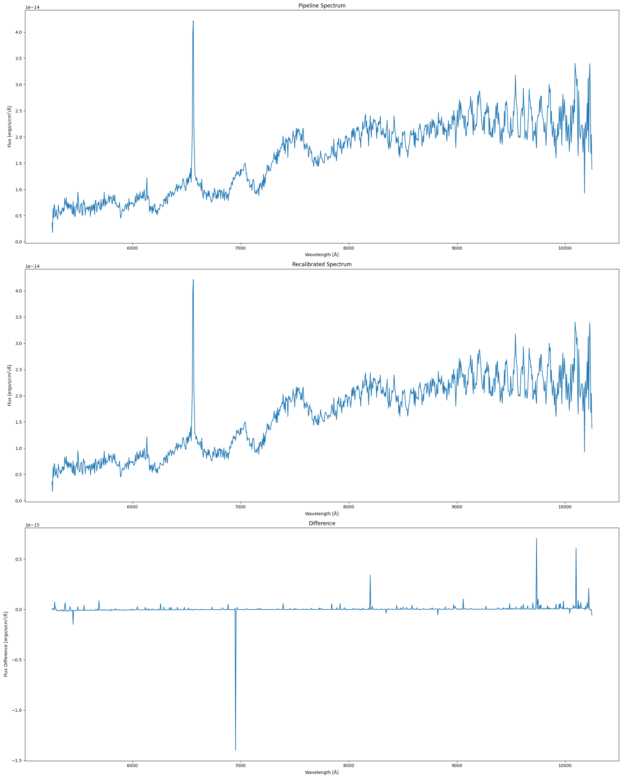
We can also visualize the flux difference in the _sx1 spectra in which we substrct the recalibrated spectrum by the pipeline spectrum:

plt.figure(figsize=(20, 25))
# get the spectrum of the default pipline _sx1 data
pip = Table.read("./mastDownload/HST/oeik1s030/oeik1s030_sx1.fits", 1)
wl, pip_flux = pip[0]["WAVELENGTH", "FLUX"]
# get the flux of the customized new_dark _sx1 data
cus = Table.read("./new_dark/oeik1s030_sx1.fits", 1)
cus_wl, cus_flux = cus[0]["WAVELENGTH", "FLUX"]
# interpolant flux so that the wavelengths matches
interp_flux = np.interp(wl, cus_wl, cus_flux)
# plot the pipeline spectrum
plt.subplot(3, 1, 1)
plt.plot(wl, pip_flux)
plt.xlabel("Wavelength [Å]")
plt.ylabel("Flux [ergs/s/cm$^2$/Å]")
plt.title("Pipeline Spectrum")
# plot the pipeline spectrum
plt.subplot(3, 1, 2)
plt.plot(cus_wl, cus_flux)
plt.xlabel("Wavelength [Å]")
plt.ylabel("Flux [ergs/s/cm$^2$/Å]")
plt.title("Recalibrated Spectrum")
# plot the spectra difference
plt.subplot(3, 1, 3)
plt.plot(wl, interp_flux-pip_flux)
plt.xlabel("Wavelength [Å]")
plt.ylabel("Flux Difference [ergs/s/cm$^2$/Å]")
plt.title("Difference")
plt.tight_layout()

About this Notebook #

Author: Keyi Ding

Updated On: 2023-04-14

This tutorial was generated to be in compliance with the STScI style guides and would like to cite the Jupyter guide in particular.

Citations #

If you use astropy, matplotlib, astroquery, or numpy for published research, please cite the authors. Follow these links for more information about citations:

Top of Page