Optimizing Image Alignment for Multiple HST Visits

This notebook requires creating and activating a virtual environment using the requirements file in this notebook's repository. Please also review the README file before using the notebook.

Table of Contents

Introduction

1. Download the Observations with astroquery

    1.1 Check image header data
    1.2 Inspect the alignment

2. Align with TweakReg

    2.1 First test: Use ‘default’ parameters
    2.2 Second test: Set parameters for source finding
    2.3 Inspect the quality of the fit

3. Combine the Images using AstroDrizzle

    3.1 Inspect the drizzled science image
    3.2 Inspect the final weight image
    3.3 Discussion of AstroDrizzle

The following Python packages are required to run the Jupyter Notebook:

• glob - gather lists of filenames

• os - change and make directories

• shutil - perform high-level file operations

• iPython - interactive handling

• matplotlib - create graphics

• numpy - math and array functions

• astropy - FITS file handling and related operations

• astroquery - download data and query databases

• drizzlepac - align and combine HST images

Introduction

Table of Contents

This notebook demonstrates how to use TweakReg and AstroDrizzle tasks to align and combine images. While this example focuses on ACS/WFC data, the procedure can be almost identically applied to WFC3/UVIS images. This notebook is based on a prior example from the 2012 DrizzlePac Handbook, but has been updated for compatibility with the latest STScI software distribution.

There is a good deal of explanatory text in this notebook, and users new to DrizzlePac are encouraged to start with this tutorial. Additional DrizzlePac software documentation is available at the readthedocs webpage.

Before running the notebook, you will need to install the astroquery package, which is used to retrieve the data from the MAST archive.

Please also make sure to appropriately set your environment variables to allow Python to locate the appropriate reference files.

import glob
import os 
import shutil

from collections import defaultdict
from IPython.display import clear_output

import matplotlib.image as mpimg
import matplotlib.pyplot as plt
import numpy as np

from astropy.io import ascii, fits
from astropy.table import Table
from astropy.visualization import ZScaleInterval

from astroquery.mast import Observations

from drizzlepac import tweakreg, astrodrizzle
from drizzlepac.processInput import getMdriztabPars

%matplotlib inline
%config InlineBackend.figure_format='retina'

The following task in the stsci.skypac package can be run with TEAL:
                                    skymatch                                    

The following tasks in the drizzlepac package can be run with TEAL:
    astrodrizzle       config_testbed      imagefindpars           mapreg       
       photeq            pixreplace           pixtopix            pixtosky      
  refimagefindpars       resetbits          runastrodriz          skytopix      
     tweakback            tweakreg           updatenpol

Along with the above imports, we also set up the required local reference files.

# Set the locations of reference files to your local computer.
os.environ['CRDS_SERVER_URL'] = 'https://hst-crds.stsci.edu'
os.environ['CRDS_SERVER'] = 'https://hst-crds.stsci.edu'
os.environ['CRDS_PATH'] = './crds_cache'
os.environ['iref'] = './crds_cache/references/hst/wfc3/'
os.environ['jref'] = './crds_cache/references/hst/acs/'

1. Download the Observations with astroquery

Table of Contents

---

MAST queries may be done using query_criteria, where we specify:

    –> obs_id, proposal_id, and filters

MAST data products may be downloaded by using download_products, where we specify:

    –> products = calibrated (FLT, FLC) or drizzled (DRZ, DRC) files

    –> type = standard products (CALxxx) or advanced products (HAP-SVM)

---

In this example, we align three F606W full-frame 339 second ACS/WFC images of the globular cluster NGC 104 from ACS/CAL Program 10737. These observations were acquired over a 3-month period in separate visits and at different orientations. We will use calibrated, CTE-corrected *_flc.fits files.

        j9irw3fwq_flc.fits
        j9irw4b1q_flc.fits
        j9irw5kaq_flc.fits

Depending on your connection speed, this cell may take a few minutes to execute.

# Because the second 'FLC' file in visit W4 is part of a dithered association,
# the 'obs_id' for that assocation will need to be used instead of the individual filename.

obs_ids = ["j9irw3fwq", "j9irw4040", "j9irw5kaq"]
props = ["10737"]
filts = ["F606W"]

obsTable = Observations.query_criteria(obs_id=obs_ids, proposal_id=props, filters=filts)
products = Observations.get_product_list(obsTable)

data_prod = ["FLC"]  # ['FLC','FLT','DRC','DRZ']
data_type = ["CALACS"]  # ['CALACS','CALWF3','CALWP2','HAP-SVM']

Observations.download_products(
    products, productSubGroupDescription=data_prod, project=data_type, cache=True
)

Downloading URL https://mast.stsci.edu/api/v0.1/Download/file?uri=mast:HST/product/j9irw3fwq_flc.fits to ./mastDownload/HST/j9irw3fwq/j9irw3fwq_flc.fits ...

 [Done]

Downloading URL https://mast.stsci.edu/api/v0.1/Download/file?uri=mast:HST/product/j9irw4b1q_flc.fits to ./mastDownload/HST/j9irw4b1q/j9irw4b1q_flc.fits ...

 [Done]

Downloading URL https://mast.stsci.edu/api/v0.1/Download/file?uri=mast:HST/product/j9irw4b3q_flc.fits to ./mastDownload/HST/j9irw4b3q/j9irw4b3q_flc.fits ...

 [Done]

Downloading URL https://mast.stsci.edu/api/v0.1/Download/file?uri=mast:HST/product/j9irw5kaq_flc.fits to ./mastDownload/HST/j9irw5kaq/j9irw5kaq_flc.fits ...

 [Done]

Table length=4

Local Path	Status	Message	URL
str47	str8	object	object
./mastDownload/HST/j9irw3fwq/j9irw3fwq_flc.fits	COMPLETE	None	None
./mastDownload/HST/j9irw4b1q/j9irw4b1q_flc.fits	COMPLETE	None	None
./mastDownload/HST/j9irw4b3q/j9irw4b3q_flc.fits	COMPLETE	None	None
./mastDownload/HST/j9irw5kaq/j9irw5kaq_flc.fits	COMPLETE	None	None

Move the files to the local working directory.

for flc in glob.glob("./mastDownload/HST/*/*flc.fits"):
    flc_name = os.path.basename(flc)
    os.rename(flc, flc_name)
if os.path.exists("mastDownload/"):
    shutil.rmtree("mastDownload/")

Remove the second FLC file in the W4 visit to simplify the example.

if os.path.exists("j9irw4b3q_flc.fits"):
    os.remove("j9irw4b3q_flc.fits")
input_flcs = glob.glob("*flc.fits")
print(input_flcs)

['j9irw3fwq_flc.fits', 'j9irw4b1q_flc.fits', 'j9irw5kaq_flc.fits']

1.1 Check image header data

Here we will look at important keywords in the image headers

paths = sorted(glob.glob("*flc.fits"))
data = []

# select desired keywords

ext_0_kws = [
    "rootname",
    "ASN_ID",
    "TARGNAME",
    "detector",
    "filter1",
    "exptime",
    "ra_targ",
    "dec_targ",
    "date-obs",
    "postarg1",
    "postarg2",
]
ext_1_kws = ["orientat"]

#grab keywords from data

for path in paths:
    path_data = []
    for keyword in ext_0_kws:
        path_data.append(fits.getval(path, keyword, ext=0))
    for keyword in ext_1_kws:
        path_data.append(fits.getval(path, keyword, ext=1))
    data.append(path_data)

# assign keywords to Table

keywords = ext_0_kws + ext_1_kws
table = Table(
    np.array(data),
    names=keywords,
    dtype=[
        "str",
        "str",
        "str",
        "str",
        "str",
        "f8",
        "f8",
        "f8",
        "str",
        "f8",
        "f8",
        "f8",
    ],
)

table["exptime"].format = "7.1f"
table["ra_targ"].format = table["dec_targ"].format = "7.4f"
table["postarg1"].format = table["postarg2"].format = "7.3f"
table["orientat"].format = "7.2f"
table

Table length=3

rootname	ASN_ID	TARGNAME	detector	filter1	exptime	ra_targ	dec_targ	date-obs	postarg1	postarg2	orientat
str32	str32	str32	str32	str32	float64	float64	float64	str32	float64	float64	float64
j9irw3fwq	NONE	NGC104-WFC	WFC	F606W	339.0	5.6604	-72.0678	2006-05-30	0.000	0.000	-125.24
j9irw4b1q	J9IRW4040	NGC104-WFC	WFC	F606W	339.0	5.6604	-72.0678	2006-07-08	0.000	0.000	-88.60
j9irw5kaq	NONE	NGC104-WFC	WFC	F606W	339.0	5.6604	-72.0678	2006-08-31	0.000	0.000	-31.45

1.2 Inspect the Alignment

Check the active WCS solution in the image header. If the image is aligned to a catalog, list the number of matches and the fit RMS in mas.
Convert the fit RMS values to pixels for comparison with the alignment results performed later in this notebook.

# select keywords needed for alignment inspections
ext_0_kws = ["DETECTOR"]
ext_1_kws = ["WCSNAME", "NMATCHES", "RMS_RA", "RMS_DEC"]

det_scale = {"IR": 0.1283, "UVIS": 0.0396, "WFC": 0.05}  # plate scale (arcsec/pixel)

# create dictionary to store alignment keywords
format_dict = {}
col_dict = defaultdict(list)

for f in sorted(glob.glob("*fl?.fits")):
    col_dict["filename"].append(f)
    hdr0 = fits.getheader(f, 0)
    hdr1 = fits.getheader(f, 1)

    for kw in ext_0_kws:  # extension 0 keywords
        col_dict[kw].append(hdr0[kw])
    for kw in ext_1_kws:  # extension 1 keywords
        if "RMS" in kw:
            val = np.around(hdr1[kw], 1)
        else:
            val = hdr1[kw]
        col_dict[kw].append(val)

    for kw in ["RMS_RA", "RMS_DEC"]:
        val = np.round(
            hdr1[kw] / 1000.0 / det_scale[hdr0["DETECTOR"]], 2
        )  # convert RMS from mas to pixels
        col_dict[f"{kw}_pix"].append(val)

wcstable = Table(col_dict)
wcstable

Table length=3

filename	DETECTOR	WCSNAME	NMATCHES	RMS_RA	RMS_DEC	RMS_RA_pix	RMS_DEC_pix
str18	str3	str30	int64	float64	float64	float64	float64
j9irw3fwq_flc.fits	WFC	IDC_4bb1536oj-FIT_IMG_GAIAeDR3	365	14.1	13.4	0.28	0.27
j9irw4b1q_flc.fits	WFC	IDC_4bb1536oj-FIT_REL_GAIAeDR3	414	14.3	11.8	0.29	0.24
j9irw5kaq_flc.fits	WFC	IDC_4bb1536oj-FIT_IMG_GAIAeDR3	361	13.5	12.6	0.27	0.25

Here we see that the FLC images from each separate visit have each been fit to the reference catalog GAIA eDR3.

For visits w3 and w5, the WCSNAME ‘FIT_IMG_catalog’ implies that each FLC was aligned separately, whereas for visit w4, the drizzle combined image ‘j9irw4040_drc.fits’ was aligned to GAIA and the solution was propogated back to the FLC exposures. (Note that the number of matches and fit rms values are different for each FLC frame.)

For more details on absolute astrometry in HST images, see Section 4.5 in the DrizzlePac Handbook.

---

2. Align with TweakReg

Table of Contents

In order to combine multiple images into a distortion-free final drizzled product, AstroDrizzle relies on the World Coordinate System (WCS) information stored in the header of each image. Because the WCS information for an image is tied to the positions of guide stars used for the observation, each visit will have small pointing errors offsets due to the uncertainty in guide star positions.

The TweakReg software can align a set of HST images to one another with subpixel accuracy (<0.1 pixel). All input images are aligned to one chosen reference image’s WCS. The reference image is typically selected as the first image in the input list, but can be chosen explicitly via the refimage parameter, if desired.

Note that since these images are already aligned to GAIA with ~400 matches and fit RMS values ~0.2 pixels. Therefore, we simply want to check the relative alignment of the FLC frame in the individual visits W3, W4 and W5, building on the eDR3 WCS solution and then testing for any residual offsets between frames.

The TweakReg algorithm consists of a few steps:

1. Makes a catalog of source positions for each input (and reference) image using a source finding algorithm        similar to DAOFind. 
2. Converts the pixel position catalogs to sky position catalogs.
3. Finds common source positions between reference and input image catalogs.
4. Calculates the shifts, rotation, and scale needed to align sky positions of sources in the input images.
5. (Optionally) Updates the input image headers with the newly calculated WCS information.

TweakReg has numerous parameters that are listed in the documentation. For this first pass, we will run TweakReg with default parameters and show how it fails for this dataset. In subsequent attempts, we will change critical parameters and show how this improves the alignment. The 5 parameters listed below are commented out when left at their default values and uncommented when set to non-defaults.

'conv_width' : 2x FWHM (~3.5 pix for point sources in ACS/WFC or WFC3/UVIS, ~2.5 pix for WFC3/IR)
'threshold'  : Signal-to-noise above bkg. Start large and reduce until number of objects is acceptable.
'peakmax'    : Source brightness cutoff, set to avoid saturated sources. 
'searchrad'  : Search radius for finding common sources between images.
'fitgeometry': Geometry used to fit offsets, rotations and/or scale changes from the matched object lists. 
               The default `fitgeometry` of 'rscale' allows for an x/y shift, scale and rotation, and the 
               'general' fit allows for an xy/shift and an independent scale and rotation for each axis.

Note that both TweakReg and AstroDrizzle will by default load in settings from any existing .cfg files if you’ve run them before. Default parameters are restored by setting configobj = None.

2.1 First test: Use ‘default’ parameters.

NOTE: Do not actually run the cells in this example, as they will use too much memory!

The most basic, out-of-the-box call to TweakReg looks like this. You TweakReg on your list of input files.

# tweakreg.TweakReg(input_flcs)

Normally, you’ll want to do some customization though. There are a variety of parameters that can be set, see the documenation for all possibilities. Here we will set a few that are helpful. Again, because we aren’t setting any souce finding parameters in showing the basic call to TweakReg, this will likely crash your computer so don’t proceed with caution if you choose to uncomment and run the cell below.

   > 'interactive' is False by default. This switch controls whether the program stops and waits for the user to examine any generated plots before continuing on to the next image. If turned off, plots will still be displayed, but they will also be saved to disk automatically as a PNG image with an autogenerated name without requiring any user input.

   > `shiftfile` is False by default, here we have set it to true to produce an intermediate output product of a file containing the shifts.
   
   > 'outshifts' is the name of the output file created when `shiftfile` is set to True.
   
   > 'updatehdr' is False by default, and specifies whether or not to update the headers of each input image directly with the shifts that were determined. This will allow the input images to be combined by AstroDrizzle without having to provide the shiftfile as well.

There are many more parameters that can be set, but the example below shows how to run TweakReg and override some of these defaults.

# Running tweakreg with some parameters changed from their defaults.
#
# tweakreg.TweakReg(input_flcs,
#                     interactive=True,
#                     shiftfile=True,
#                     outshifts='shift_default.txt',
#                     updatehdr=False)

2.2 Second test: Set parameters for source finding

One of the crucial steps for aligning images is creating a catalog of common sources in each image to do the alignment. TweakReg uses a set of default parameters to do this source finding, but you will likely want to override these and tailor them to your dataset. As described above, using the defaults on this dataset of a cluster will simply produce too many sources and use too much memory for the average user’s machine. In this example, we will adjust some of these to parameters.

In the above example, none of the source finding parameters were adjusted. TweakReg, by default, looks for sources which are 4-sigma above the background, but this threshold value is too low, since the catalogs contain ~60,000 objects per chip in each frame, and ~6500 matched sources between each exposure. Setting the threshold to a very low value generally does not translate to a better solution, since all sources are weighted equally when computing fits to match catalogs. This is especially relevant for ACS/WFC and WFC3/UVIS data where CTE tails can shift the centroid position slightly along the readout direction for faint sources and potentially bias the fit.

In this test, the threshold value is adjusted to a larger value, and the peakmax value is set to 70,000 electrons to exclude full-well saturated objects for gain=2. TweakReg now finds a more reasonable number of sources per ACS chip (~700).

Note that there are other source finding parameters that can be adjusted and that you may need to adjust. For example, you may need to also adjust searchrad if your images have large offsets.

tweakreg.TweakReg(
    input_flcs,
    threshold=4000,
    peakmax=70000,
    configobj=None,
    interactive=False,
    shiftfile=True,
    outshifts="shift_rscale.txt",
    ylimit=0.2,
    fitgeometry="rscale",
    updatehdr=False,
    reusename=True,
)
#clear_output()

Setting up logfile :  tweakreg.log

TweakReg Version 3.7.1 started at: 16:10:05.428 (19/09/2024) 

Version Information

--------------------

Python Version 3.11.10 (main, Sep  9 2024, 03:20:25) [GCC 11.4.0]

numpy Version -> 1.26.4 

astropy Version -> 6.1.3 

stwcs Version -> 1.7.3 

photutils Version -> 1.12.0 

Finding shifts for: 

    j9irw3fwq_flc.fits

    j9irw4b1q_flc.fits

    j9irw5kaq_flc.fits

===  Source finding for image 'j9irw3fwq_flc.fits':

  #  Source finding for 'j9irw3fwq_flc.fits', EXT=('SCI', 1) started at: 16:10:05.518 (19/09/2024)

     Found 626 objects.

  #  Source finding for 'j9irw3fwq_flc.fits', EXT=('SCI', 2) started at: 16:10:05.88 (19/09/2024)

     Found 408 objects.

===  FINAL number of objects in image 'j9irw3fwq_flc.fits': 1034

===  Source finding for image 'j9irw4b1q_flc.fits':

  #  Source finding for 'j9irw4b1q_flc.fits', EXT=('SCI', 1) started at: 16:10:06.57 (19/09/2024)

     Found 708 objects.

  #  Source finding for 'j9irw4b1q_flc.fits', EXT=('SCI', 2) started at: 16:10:06.942 (19/09/2024)

     Found 398 objects.

===  FINAL number of objects in image 'j9irw4b1q_flc.fits': 1106

===  Source finding for image 'j9irw5kaq_flc.fits':

  #  Source finding for 'j9irw5kaq_flc.fits', EXT=('SCI', 1) started at: 16:10:07.6 (19/09/2024)

     Found 524 objects.

  #  Source finding for 'j9irw5kaq_flc.fits', EXT=('SCI', 2) started at: 16:10:07.961 (19/09/2024)

     Found 343 objects.

===  FINAL number of objects in image 'j9irw5kaq_flc.fits': 867

===============================================================

Performing alignment in the projection plane defined by the WCS

derived from 'j9irw3fwq_flc.fits'

===============================================================

====================

Performing fit for: j9irw4b1q_flc.fits

Matching sources from 'j9irw4b1q_flc.fits' with sources from reference image 'j9irw3fwq_flc.fits'

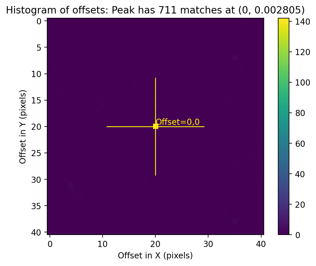
Computing initial guess for X and Y shifts...

Found initial X and Y shifts of -0.001445, -0.00289 with significance of 668.5 and 692 matches

Found 691 matches for j9irw4b1q_flc.fits...

Computed  rscale  fit for  j9irw4b1q_flc.fits : 

XSH: -0.0137  YSH: 0.0088    ROT: 0.0007210868143    SCALE: 0.999996

FIT XRMS: 0.042      FIT YRMS: 0.041  

FIT RMSE: 0.059      FIT MAE: 0.052  

RMS_RA: 5e-07 (deg)   RMS_DEC: 8e-07 (deg)

Final solution based on  681  objects.

wrote XY data to:  j9irw4b1q_flc_catalog_fit.match

Total # points: 681

# of points after clipping: 681

Total # points: 681

# of points after clipping: 681

====================

Performing fit for: j9irw5kaq_flc.fits

Matching sources from 'j9irw5kaq_flc.fits' with sources from reference image 'j9irw3fwq_flc.fits'

Computing initial guess for X and Y shifts...

Found initial X and Y shifts of 3.553e-15, 0.002805 with significance of 690.5 and 713 matches

Found 713 matches for j9irw5kaq_flc.fits...

Computed  rscale  fit for  j9irw5kaq_flc.fits : 

XSH: 0.0730  YSH: -0.0325    ROT: 0.0003022339433    SCALE: 1.000010

FIT XRMS: 0.05       FIT YRMS: 0.047  

FIT RMSE: 0.068      FIT MAE: 0.061  

RMS_RA: 5.3e-07 (deg)   RMS_DEC: 9.3e-07 (deg)

Final solution based on  702  objects.

wrote XY data to:  j9irw5kaq_flc_catalog_fit.match

Total # points: 702

# of points after clipping: 702

Total # points: 702

# of points after clipping: 702

Writing out shiftfile : shift_rscale.txt

Trailer file written to:  tweakreg.log

# If the alignment is unsuccessful, stop the notebook
with open("shift_rscale.txt", "r") as shift:
    for line_number, line in enumerate(shift, start=1):
        if "nan" in line:
            raise ValueError("nan found in line {} in shift file".format(line_number))

2.3 Inspect the quality of the fit

In your work, you will likely have to play around with TweakReg parameters to find the optimal set for your data. This requires inspecting the quality of the fit after each run. If you scroll to the bottom of the last cell run, you can see some diagnostic plots there including a residual and vector plot that show the quality of fit. Here, we will inspect some of the outputs that are saved.

The shift file below shows that the xrms and yrms of the computed fit are excellent, around ~0.04 pixels.

# create Table from shift_rscale.txt
shift_tab = Table.read(
    "shift_rscale.txt",
    format="ascii.no_header",
    names=["file", "dx", "dy", "rot", "scale", "xrms", "yrms"],
)

formats = [".2f", ".2f", ".3f", ".5f", ".2f", ".2f"]
for i, col in enumerate(shift_tab.colnames[1:]):
    shift_tab[col].format = formats[i]
shift_tab

Table length=3

file	dx	dy	rot	scale	xrms	yrms
str18	float64	float64	float64	float64	float64	float64
j9irw3fwq_flc.fits	0.00	0.00	0.000	1.00000	0.00	0.00
j9irw4b1q_flc.fits	-0.01	0.01	0.001	1.00000	0.04	0.04
j9irw5kaq_flc.fits	0.07	-0.03	0.000	1.00001	0.05	0.05

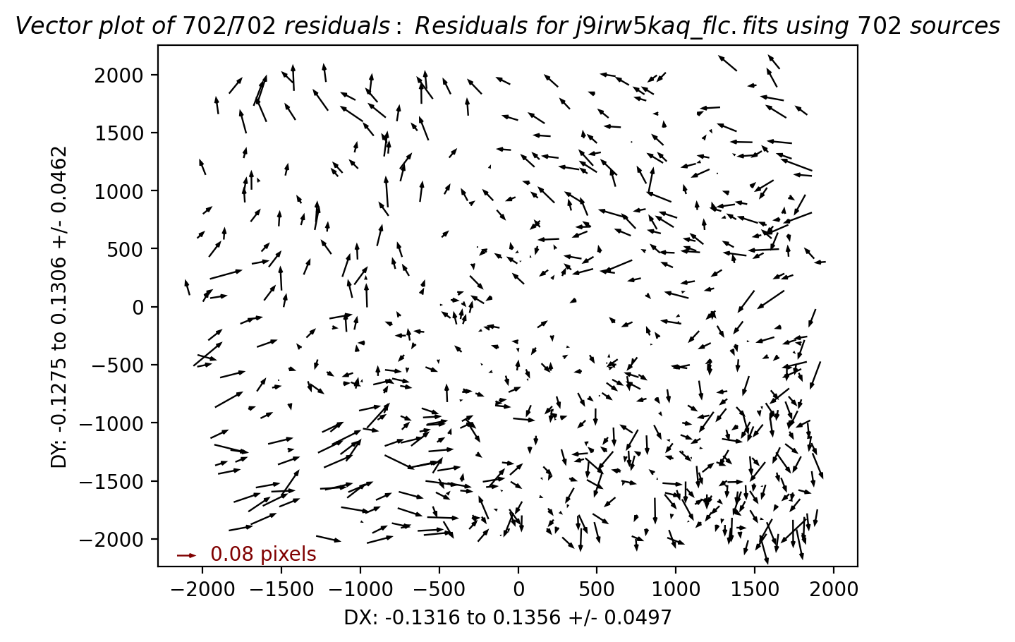
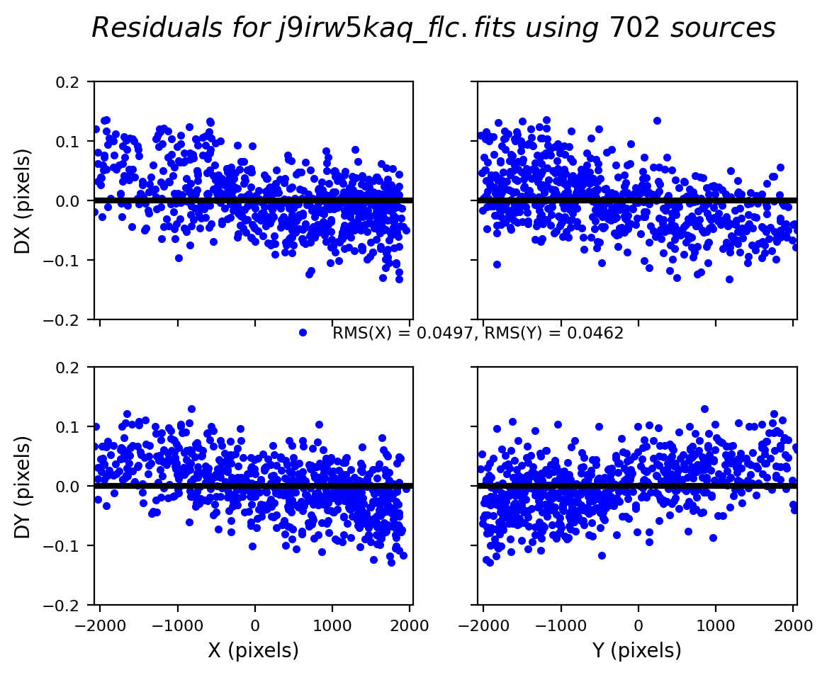
When interactive = False, TweakReg outputs several diagnostic plots in the working directory for you to inspect the fit quality. For each input file, except the reference file, TweakReg creates an x/y plot of fit residuals and a vector plot. Let’s take a look at these.

# Give the 'fit residual plots' a unique name for comparison with other tests.
rootname_A = "j9irw4b1q"
rootname_B = "j9irw5kaq"

# make a subdirectory for storing images
os.makedirs("images", exist_ok=True)
shutil.copy(f"residuals_{rootname_A}_flc.png", f"images/residuals_{rootname_A}_flc_rscale.png")
shutil.copy(f"residuals_{rootname_B}_flc.png", f"images/residuals_{rootname_B}_flc_rscale.png")

shutil.copy(f"vector_{rootname_A}_flc.png", f"images/vector_{rootname_A}_flc_rscale.png")
shutil.copy(f"vector_{rootname_B}_flc.png", f"images/vector_{rootname_B}_flc_rscale.png")

'images/vector_j9irw5kaq_flc_rscale.png'

# read images
img_A = mpimg.imread(f"images/residuals_{rootname_A}_flc_rscale.png")
img_B = mpimg.imread(f"images/residuals_{rootname_B}_flc_rscale.png")

# display images
fig, axs = plt.subplots(1, 2, figsize=(10, 10), dpi=200)
axs[0].imshow(img_A)
axs[1].imshow(img_B)
axs[0].axis("off")
axs[1].axis("off")
fig.tight_layout()

plt.show()

# read images
img_A = mpimg.imread(f"images/vector_{rootname_A}_flc_rscale.png")
img_B = mpimg.imread(f"images/vector_{rootname_B}_flc_rscale.png")

# display images
fig, axs = plt.subplots(1, 2, figsize=(10, 10), dpi=100)
axs[0].imshow(img_A)
axs[1].imshow(img_B)
axs[0].axis("off")
axs[1].axis("off")
fig.tight_layout()
plt.show()

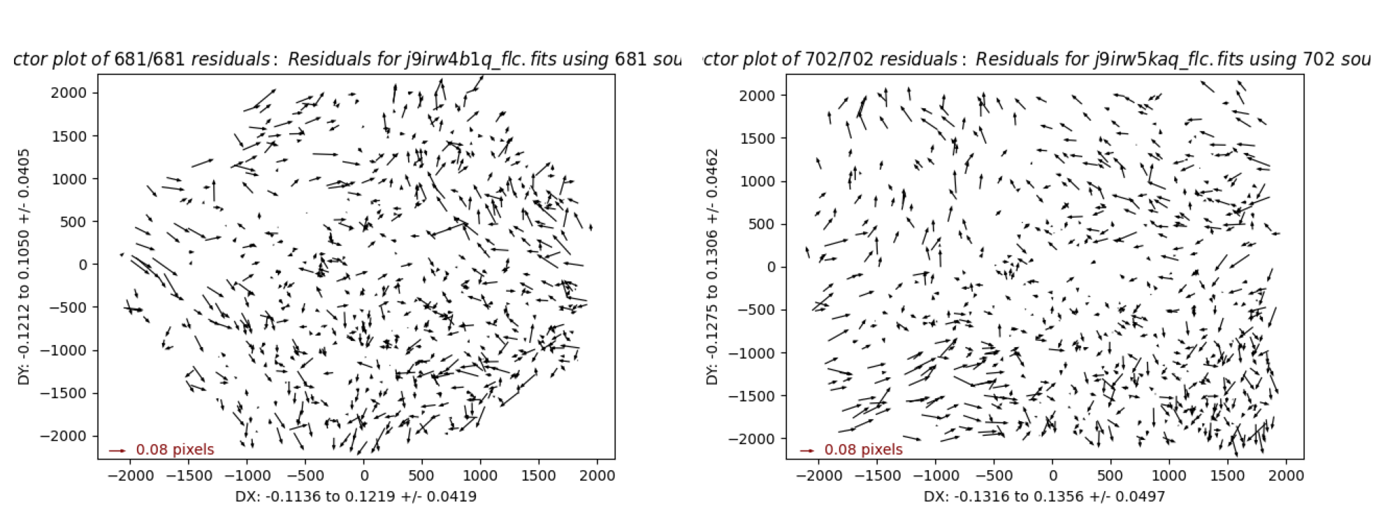
The residual plots show a fit RMS of ~0.04 pixels, but there is still a systematic skew in the fit residuals, which is believed to be caused by an uncorrected ‘skew’ in the ACS distortion solution.

As of creation of this notebook in 2024, the following calibration reference files were used:

• IDCTAB = ‘jref$4bb1536oj_idc.fits’ / Image Distortion Correction Table

• D2IMFILE = ‘jref$4bb15371j_d2i.fits’ / Column Correction Reference File

• NPOLFILE = ‘jref$4bb1536ej_npl.fits’ / Non-polynomial Offsets Reference File (F606W)

New distortion solutions are in the process of being derived by the ACS team, so observations retrieved from MAST at a later date may or may not show these systematic skew residuals. Fortunately, these can be corrected by allowing for a higher order fitgeometry as shown in the next test.

More information about the distortion reference files used by AstroDrizzle may be found in the DrizzlePac Handbook Section 4.3.

2.4 Fourth test: Adjust the fitgeometry

In this test, the fitgeometry parameter is changed from the default rscale (shift, rotation, scale) to general (shift, xrot, yrot, xscale, yscale) in order to correct for residual skew terms.

# run TweakReg
tweakreg.TweakReg(
    input_flcs,
    threshold=4000,
    peakmax=70000,
    configobj=None,
    interactive=False,
    shiftfile=True,
    outshifts="shift_general.txt",
    ylimit=0.2,
    fitgeometry="general",
    updatehdr=False,
    reusename=True
)
clear_output()

# create Table from shift_rscale.txt
shift_tab = Table.read(
    "shift_general.txt",
    format="ascii.no_header",
    names=["file", "dx", "dy", "rot", "scale", "xrms", "yrms"],
)

formats = [".2f", ".2f", ".3f", ".5f", ".2f", ".2f"]
for i, col in enumerate(shift_tab.colnames[1:]):
    shift_tab[col].format = formats[i]
shift_tab

Table length=3

file	dx	dy	rot	scale	xrms	yrms
str18	float64	float64	float64	float64	float64	float64
j9irw3fwq_flc.fits	0.00	0.00	0.000	1.00000	0.00	0.00
j9irw4b1q_flc.fits	-0.01	0.01	0.001	0.99999	0.03	0.03
j9irw5kaq_flc.fits	0.07	-0.02	0.000	1.00001	0.04	0.03

# Print the number of matches for images 2 and 3 with respect to image1
rootname2 = "j9irw4b1q"
rootname3 = "j9irw5kaq"
match_tab2 = ascii.read(
    rootname2 + "_flc_catalog_fit.match"
)  # load match file in astropy table
match_tab3 = ascii.read(
    rootname3 + "_flc_catalog_fit.match"
)  # load match file in astropy table
print(rootname2, "     Number of Gaia Matches=", {len(match_tab2)})
print(rootname3, "     Number of Gaia Matches=", {len(match_tab3)})

j9irw4b1q      Number of Gaia Matches= {681}
j9irw5kaq      Number of Gaia Matches= {705}

# Compare with the MAST solutions
wcstable

Table length=3

filename	DETECTOR	WCSNAME	NMATCHES	RMS_RA	RMS_DEC	RMS_RA_pix	RMS_DEC_pix
str18	str3	str30	int64	float64	float64	float64	float64
j9irw3fwq_flc.fits	WFC	IDC_4bb1536oj-FIT_IMG_GAIAeDR3	365	14.1	13.4	0.28	0.27
j9irw4b1q_flc.fits	WFC	IDC_4bb1536oj-FIT_REL_GAIAeDR3	414	14.3	11.8	0.29	0.24
j9irw5kaq_flc.fits	WFC	IDC_4bb1536oj-FIT_IMG_GAIAeDR3	361	13.5	12.6	0.27	0.25

While the shift file looks nearly identical to the prior run, this is because the axis-dependent rotation and scale values are averaged together in the shiftfile. To determine the actual values, it is necessary to inspect the ‘tweakreg.log’ logfile.

j9irw4b1q  SCALE_X: 0.9999720117  SCALE_Y: 1.000014811  ROT_X: 359.9999  ROT_Y:   0.0014   SKEW: -359.9985
j9irw5kaq  SCALE_X: 0.9999851345  SCALE_Y: 1.000030317  ROT_X:   0.0015  ROT_Y: 359.9989   SKEW:  359.9974

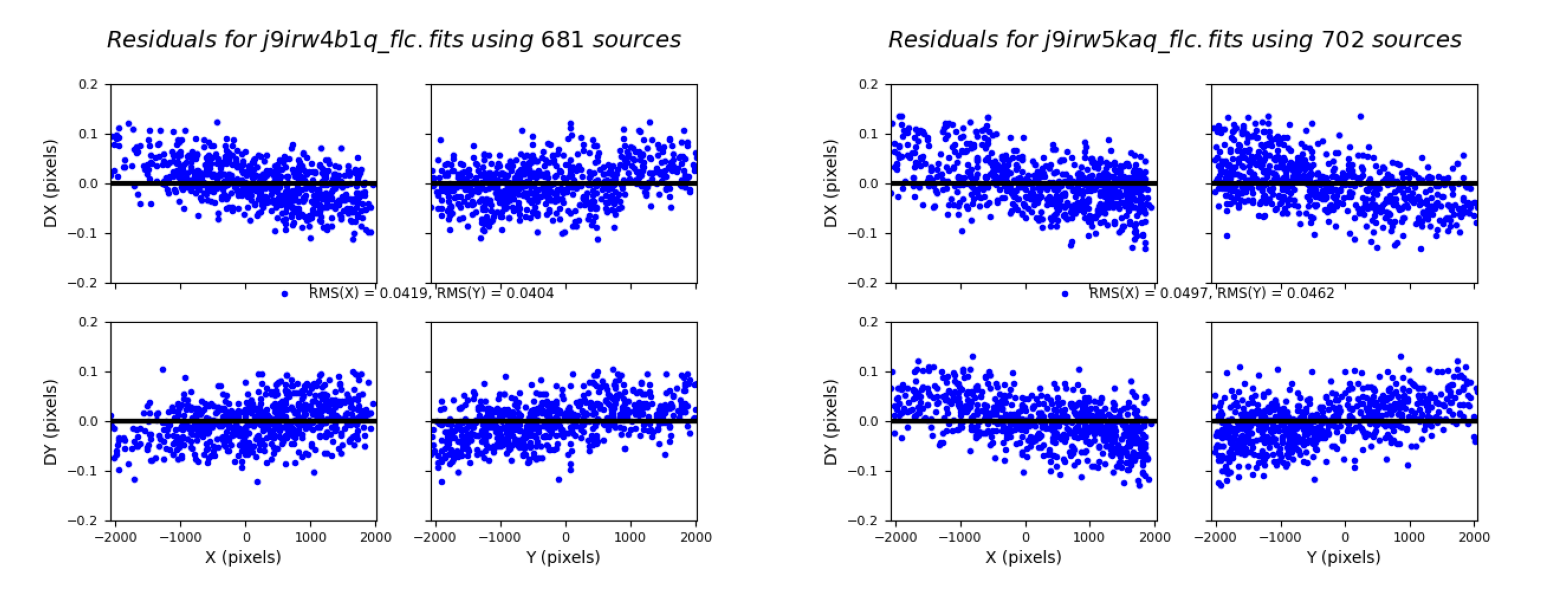
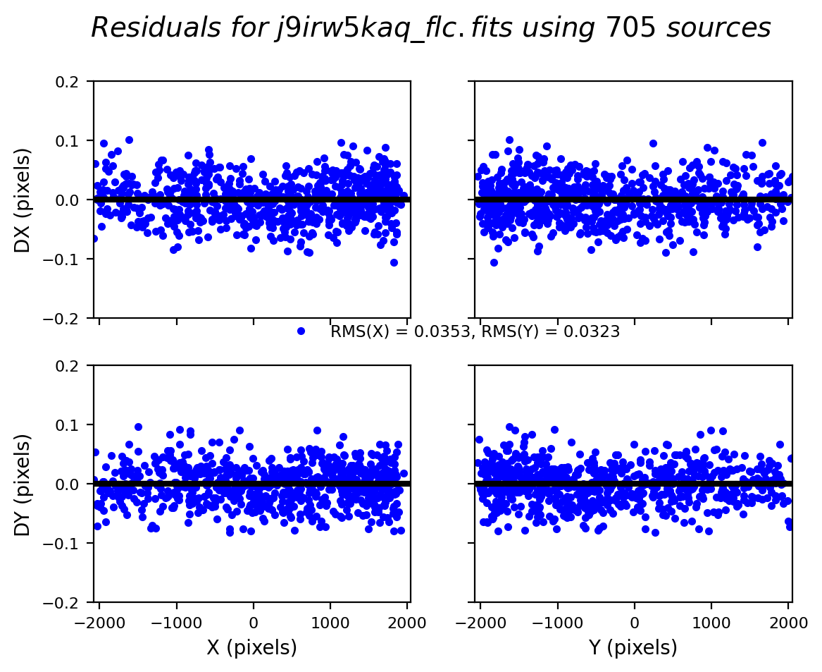
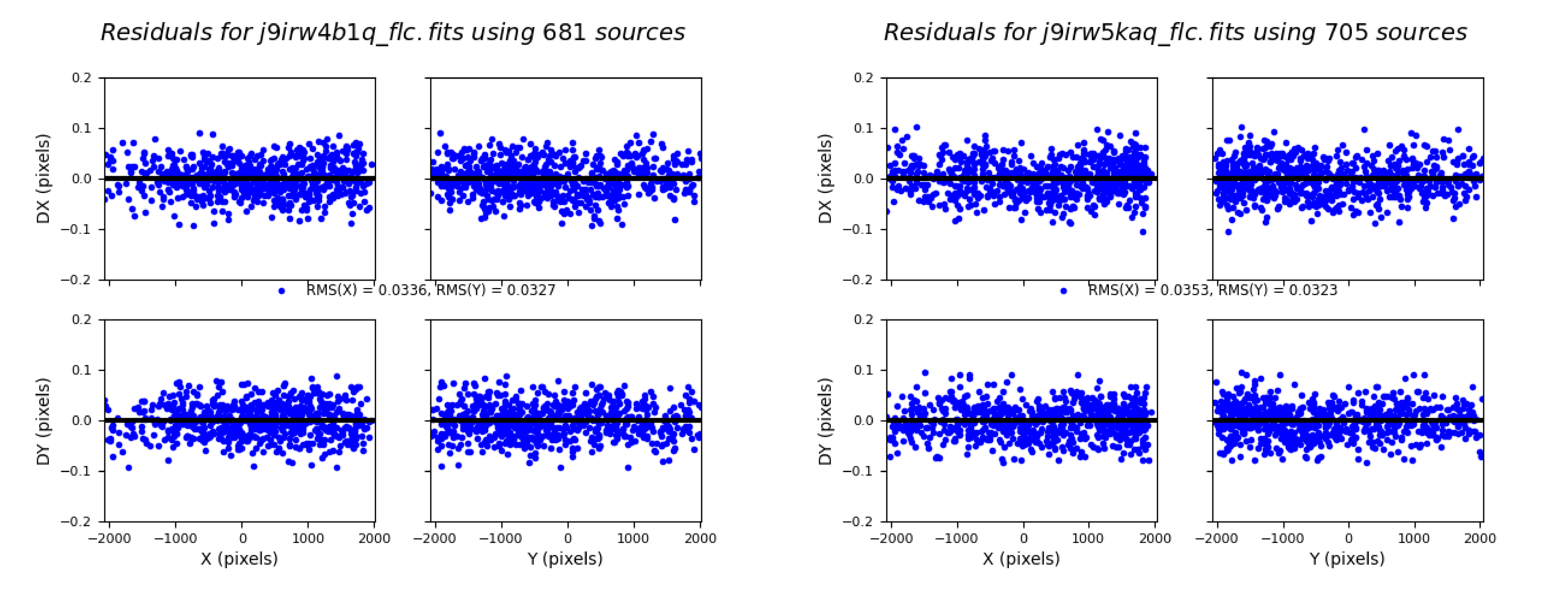
The ‘general’ fit reduces the fit rms to ~0.03 pixels from the prior value of ~0.05 pixels and removes systematics from the residuals in the plots below.

# Give the 'fit residual plots' a unique name for comparison with other tests.
shutil.copy(f"residuals_{rootname_A}_flc.png", f"images/residuals_{rootname_A}_flc_general.png")
shutil.copy(f"residuals_{rootname_B}_flc.png", f"images/residuals_{rootname_B}_flc_general.png")

shutil.copy(f"vector_{rootname_A}_flc.png", f"images/vector_{rootname_A}_flc_general.png")
shutil.copy(f"vector_{rootname_B}_flc.png", f"images/vector_{rootname_B}_flc_general.png")

'images/vector_j9irw5kaq_flc_general.png'

The plots below shows residuals in X and Y plotted as functions of X and Y. Each point represents a source that was used for the alignment. The residuals should look fairly random - if any correlation is seen, this is an indicator of a poor alignment solution. In some cases you will notice a wavy pattern in the residuals in X and Y. This is often seen for UVIS images and is a result of lithographic patterns of the detector that are not fully corrected for in the distortion solutions. The RMS in X and Y are also printed. For a good alignment, we are looking for an RMS on the order of 0.1 pixel or less.

# read images
img_A = mpimg.imread(f"images/residuals_{rootname_A}_flc_general.png")
img_B = mpimg.imread(f"images/residuals_{rootname_B}_flc_general.png")

# display images
fig, axs = plt.subplots(1, 2, figsize=(20, 10), dpi=200)
axs[0].imshow(img_A)
axs[1].imshow(img_B)
axs[0].axis("off")
axs[1].axis("off")
fig.tight_layout()
plt.show()

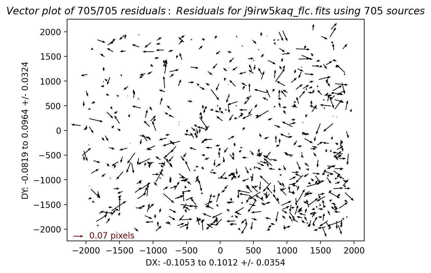
# read images
img_A = mpimg.imread(f"images/vector_{rootname_A}_flc_general.png")
img_B = mpimg.imread(f"images/vector_{rootname_B}_flc_general.png")

# display images
fig, axs = plt.subplots(1, 2, figsize=(10, 10), dpi=100)
axs[0].imshow(img_A)
axs[1].imshow(img_B)
axs[0].axis("off")
axs[1].axis("off")
fig.tight_layout()
plt.show()

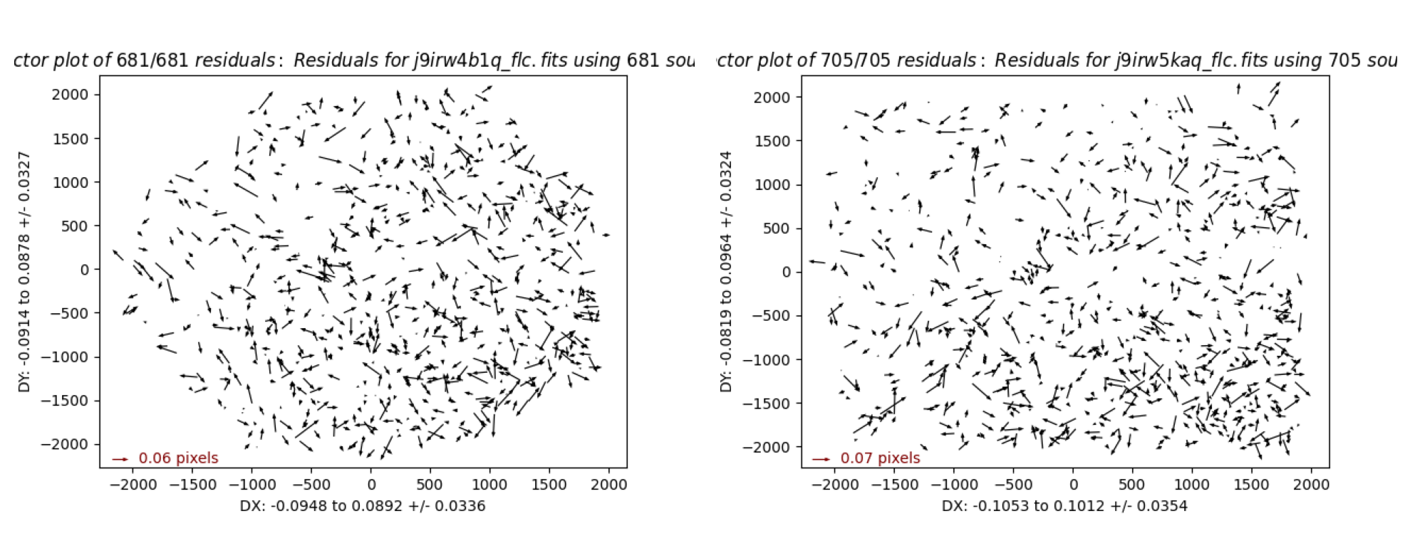
The direction and the magnitude of the arrows in the vector plot above represent the offsets in the source position between the image in question and the reference image. These should visually appear random if the alignment was sucessful.

You may need to run TweakReg run several times with varying parameters until a good fit is found. Notice in the above tests that updatehdr = False. This allows you to attempt the alignment and inspect the results without actually updating the WCS to solidify the alignment. Once you are satisfied with the results, TweakReg is run a final time with updatehdr = True, and a new WCS will be inserted in the file. The default name of this new WCS is ‘TWEAK’, but can be changed by setting the wcsname.

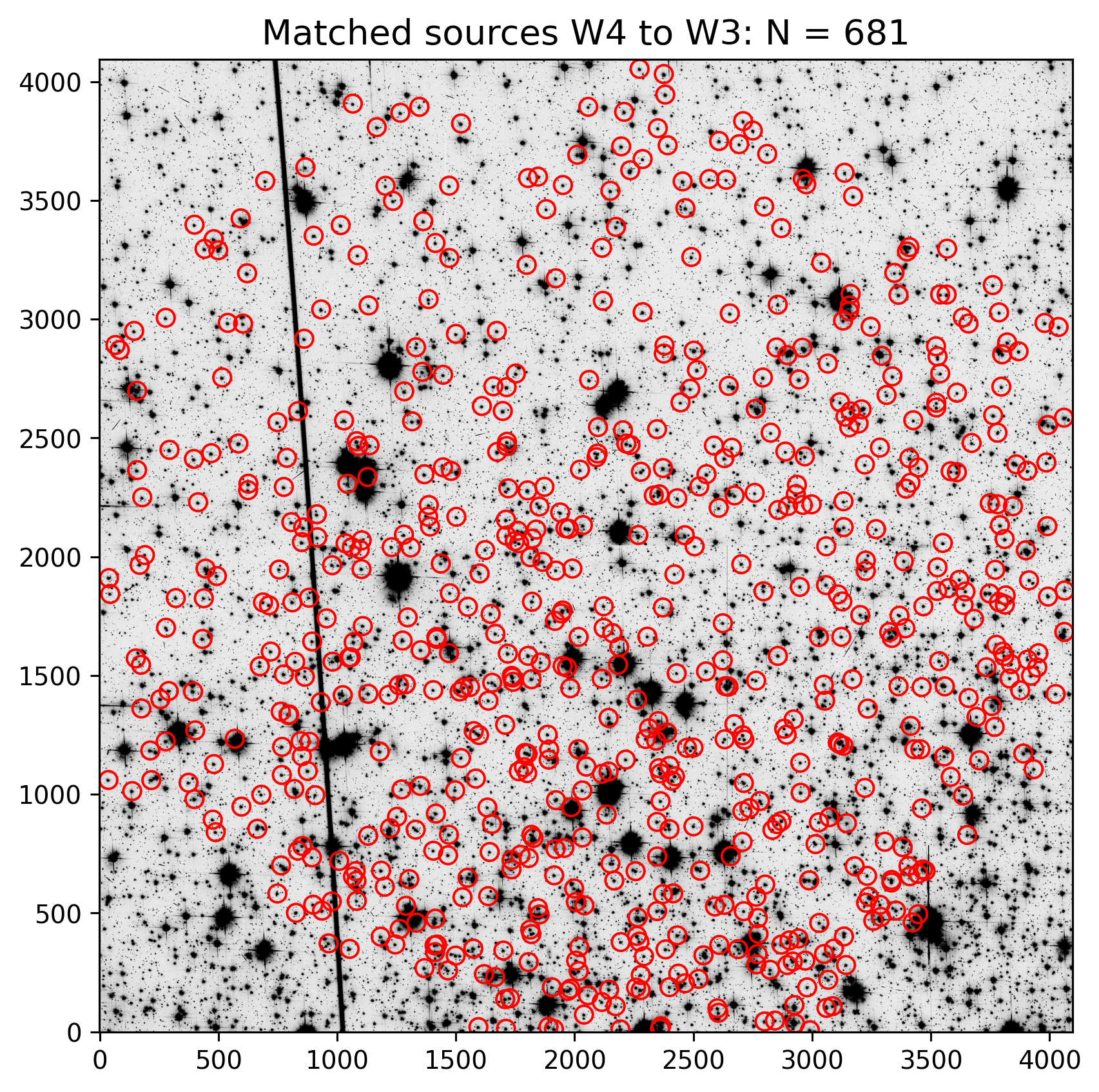
2.5 Overplot Matched Sources on the Image

As a final quality check before updating the image header WCS, we plot the sources that were matched between FLC images in visits W3 and W4.

The cell below shows how to read in the *_fit.match file as an astropy table. Unfortunately, it doesn’t automatically name columns so you’ll have to look at the header to grab the columns.

rootname = "j9irw4b1q"

plt.figure(figsize=(7, 7), dpi=140)

with fits.open(rootname + "_flc.fits") as hdulist: 
    chip1_data = hdulist["SCI", 2].data 
    chip2_data = hdulist["SCI", 1].data
    fullsci = np.concatenate([chip2_data, chip1_data])
    zscale = ZScaleInterval()
    z1, z2 = zscale.get_limits(fullsci)
    plt.imshow(fullsci, cmap="Greys", origin="lower", vmin=z1, vmax=z2)
    
    match_tab = ascii.read(
        rootname + "_flc_catalog_fit.match"
    )  # load match file in astropy table
    match_tab_chip1 = match_tab[
        match_tab["col15"] == 2
    ]  # filter table for sources on chip 1 (on ext 4)
    match_tab_chip2 = match_tab[
        match_tab["col15"] == 1
    ]  # filter table for sources on chip 1 (on ext 4)
    x_cord1, y_cord1 = match_tab_chip1["col11"], match_tab_chip1["col12"]
    x_cord2, y_cord2 = match_tab_chip2["col11"], match_tab_chip2["col12"]
    
    plt.scatter(
        x_cord1,
        y_cord1 + 2051,
        s=50,
        edgecolor="r",
        facecolor="None",
        label="Matched Sources",
    )
    plt.scatter(x_cord2, y_cord2, s=50, edgecolor="r", facecolor="None")
    plt.title(
        f"Matched sources W4 to W3: N = {len(match_tab)}", fontsize=14
    )
    plt.show()

2.6 Update header once optimal parameters are found

Once you’ve decided on the optimal set of parameters for your alignment, it is safe to update the header of the input data. Note that because the first image is already aligned to Gaia, this does not need to be done again and we focus only on improving the relative alignment.

tweakreg.TweakReg(
    input_flcs,
    threshold=4000,
    peakmax=70000,
    configobj=None,
    interactive=False,
    shiftfile=False,
    ylimit=0.2,
    fitgeometry="general",
    updatehdr=True, # update the header with the new solution
    reusename=True
)  

clear_output()

3. Combine the Images using AstroDrizzle

Table of Contents

Now that the images are aligned to a common WCS, they are ready for combination with AstroDrizzle. All of the input exposures taken in a single filter will contribute to a single drizzled output file.

The AstroDrizzle steps after alignment are summarized below.

1. A static pixel mask is created to flag bad detector pixels.
2. Sky subtraction is performed on masked images. 
3. Each image is individually drizzled, with geometric distortion corrections, to a common reference frame.
4. The distortion-free drizzled images are combined to create a median image.
5. The median image is blotted, or reverse-drizzled, back to the frame of each input image.
6. By comparing each input image with its counterpart blotted median image, the software locates bad pixels in each of the original frames & creates bad pixel masks (typically CR's and bad pixels in the detector)
7. In the final step, input images are drizzled together onto a single output image.

Let’s first run AstroDrizzle on the aligned input images in the next cell to create a combined image f606w_combined_drc, then go into further detail about the drizzle process.

Note that astrodrizzle supports the loading of a custom configuration file (.cfg) files, but we will be using the command-line syntax interface to set the parameters in this example, where parameters are passed into the function directly. Any existing .cfg file will be overridden by setting configobj = None so that unless explicitly set, parameters will be reset to default.

First, we get some recommended values for drizzling from the MDRIZTAB reference file. The parameters in this file are different for each detector and are based on the number of input frames. These are a good starting point for drizzling and may be adjusted accordingly.

# The following lines of code find and download the MDRIZTAB reference file.
mdz = fits.getval(input_flcs[0], 'MDRIZTAB', ext=0).split('$')[1]
jref = os.environ['jref']
print('Searching for the MDRIZTAB file:', mdz)
!crds sync --hst --files {mdz} --output-dir {jref}

Searching for the MDRIZTAB file: 37g1550cj_mdz.fits

CRDS - INFO -  Symbolic context 'hst-operational' resolves to 'hst_1181.pmap'
CRDS - INFO -  Reorganizing 0 references from 'instrument' to 'flat'
CRDS - INFO -  Reorganizing from 'instrument' to 'flat' cache,  removing instrument directories.
CRDS - INFO -  Syncing explicitly listed files.

CRDS - INFO -  Fetching  ./crds_cache/references/hst/acs/37g1550cj_mdz.fits       247.7 K bytes  (1 / 1 files) (0 / 247.7 K bytes)

CRDS - INFO -  0 errors
CRDS - INFO -  0 warnings
CRDS - INFO -  5 infos

def get_vals_from_mdriztab(
    input_flcs,
    kw_list=[
        "driz_sep_bits",
        "combine_type",
        "driz_cr_snr",
        "driz_cr_scale",
        "final_bits",
    ],
):
    """Get only selected parameters from. the MDRIZTAB"""
    mdriz_dict = getMdriztabPars(input_flcs)

    requested_params = {}

    print("Outputting the following parameters:")
    for k in kw_list:
        requested_params[k] = mdriz_dict[k]
        print(k, mdriz_dict[k])

    return requested_params

selected_params = get_vals_from_mdriztab(input_flcs)

- MDRIZTAB: AstroDrizzle parameters read from row 2.
Outputting the following parameters:
driz_sep_bits 336
combine_type minmed
driz_cr_snr 3.5 3.0
driz_cr_scale 1.5 1.2
final_bits 336

Note that the parameter final_bits= ‘336’ is equivalent to final_bits= ‘256, 64, 16’.

Since the ACS team now corrects for stable hot pixels (DQ flag=16) via the dark reference files, these pixels can be considered ‘good’. Full well saturated pixels (DQ flag=256) and warm pixels (DQ flag=64) may also be treated as good. More details on the recommended drizzle parameters for ACS may be found in ISR 2017-02.

Next we run AstroDrizzle to remove the sky, flag cosmic rays, and combine the image using the selected parameters. Note that these may be further refined by uncommenting the lines in the example shown below.

# To override any of the above values, e.g.:
# selected_params["driz_sep_bits"] = "256, 64, 16"
# selected_params["final_bits"] = "256, 64, 16"

astrodrizzle.AstroDrizzle(
    input_flcs,
    output="f606w_combined",
    preserve=False,
    build=True,
    skymethod="match",
    driz_sep_bits=selected_params["driz_sep_bits"],
    driz_cr_corr=True,
    clean=False,
    final_bits=selected_params["final_bits"],
    configobj=None,
)
clear_output()

You will see the following files (among others) output by AstroDrizzle in the working directory.

1. ‘f606w_combined_drc.fits’ : Multi-extension FITS file.

   When build = True, the drizzled science image, context image, weight image, and median image will be combined into a single multi-extension fits file. This file contains the following extensions:

    Final drizzled science image is contained in ['SCI', 1].
    Final drizzled weight  image is contained in ['WHT', 1].
    Final drizzled context image is contained in ['CTX', 1].
   

   When build = False, these will be output as separate files (_sci.fits, _wht.fits, _ctx.fits).

   When final_wht_type = EXP (default), the weight image it is effectively an exposure time map of each pixel in the final drizzled image. Other options are error ‘ERR’ and inverse variance ‘IVM’ weighting, as described in more detail here.

   The context image is a map showing which images contribute to the final drizzled stack. Each input image chip is identified by a bit in a 32-bit integer. For example, image1/chip1 = 2^0 = 1, image1/chip2 = 2^1 = 2. Each context image pixel is an additive combination of these bits, depending on which images contributed to the corresponding pixel in the drizzled image.

2. astrodrizzle.log : Log file containing details of the drizzle processing steps.

3. f606w_combined_med.fits : Median image computed from the sky-subtracted, separately-drizzled input images.

4. j*_crclean.fits : Cosmic-ray cleaned versions of the original input flc images.

Because we set clean = False, there will be various other intermediate output files in the directory, including masks, blotted frames, etc. This behavior can be modified with the clean and in_memory parameters.

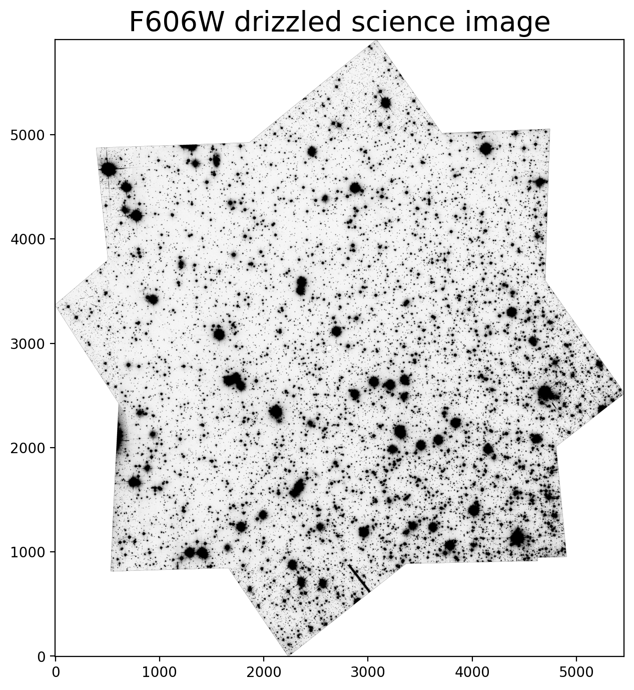
3.1 Inspect the drizzled science image

Finally, we inspect the science and weight images and inspect their data quality. An imprint of sources in the weight image may indicate an error with the alignment and subsequent cosmic-ray rejection.

For more details on inspecting the drizzled products after reprocessing, see Section 7.3 in the DrizzlePac Handbook

plt.figure(figsize=(8, 8))

with fits.open("f606w_combined_drc.fits") as hdulist: 
    drc_dat = hdulist["SCI", 1].data # final drizzled image in SCI,1 extension
    
    z1, z2 = zscale.get_limits(drc_dat)
    plt.imshow(drc_dat, origin="lower", vmin=z1, vmax=z2, cmap="Greys")
    plt.title("F606W drizzled science image", fontsize=20)
    plt.show()

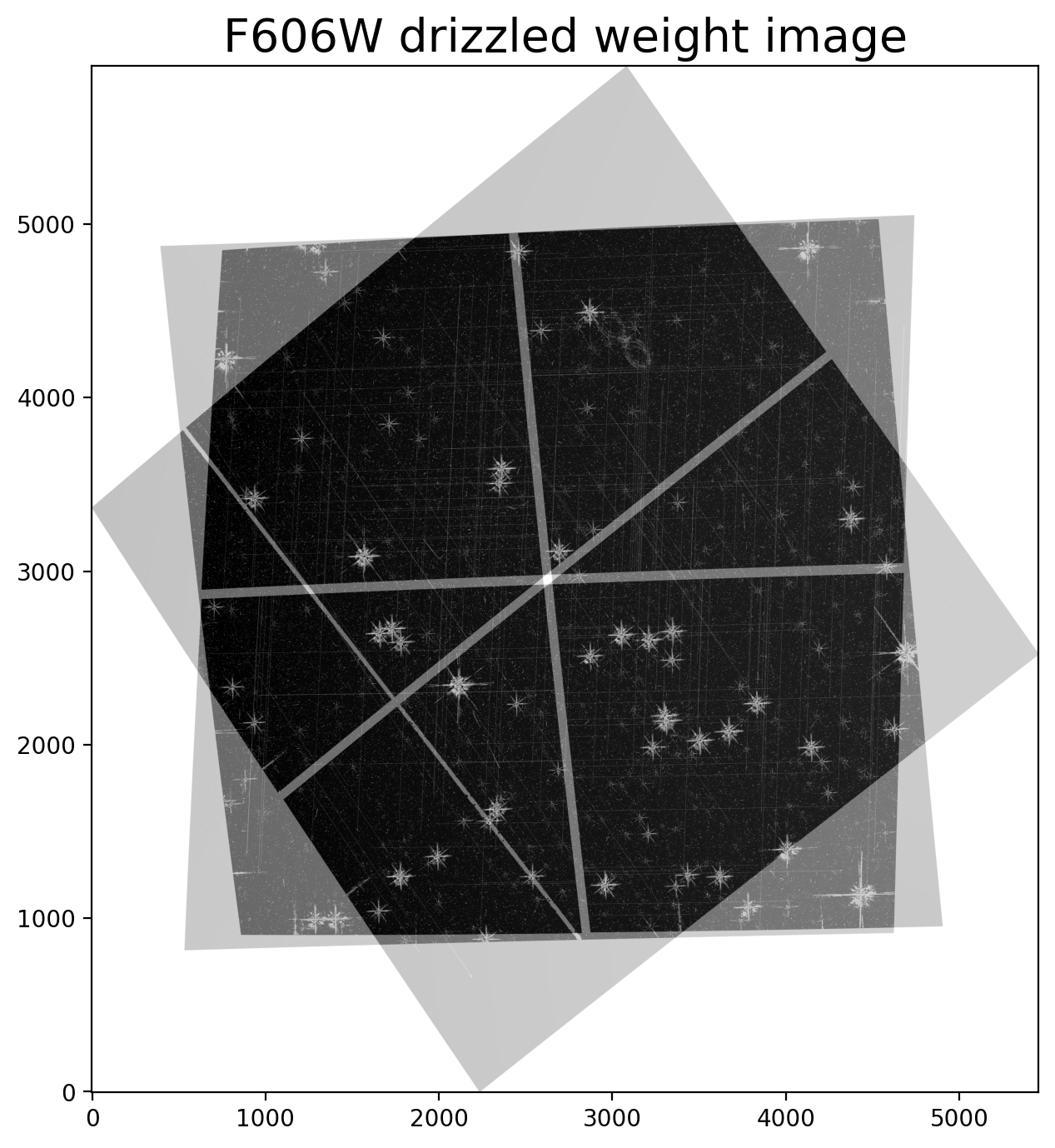
3.2 Inspect the final weight image

plt.figure(figsize=(8, 8))

with fits.open("f606w_combined_drc.fits") as hdulist: 
    drc_dat = hdulist["WHT", 1].data # final drizzled image in WHT,1 extension

    z1, z2 = zscale.get_limits(drc_dat)
    plt.imshow(drc_dat, origin="lower", vmin=z1, vmax=z2, cmap="Greys")
    plt.title("F606W drizzled weight image", fontsize=20)
    plt.show()

3.3 Discussion of AstroDrizzle and Summary

In this example, we imported and ran the AstroDrizzle task on our input images, which were previously aligned with TweakReg. By setting configobj to None, we ensured that AstroDrizzle was not picking up any existing configuration files and parameters were restored to default values. We then set a select few parameters to non-default values:

1. output = 'f606w_combined' : Output file name root (which will be appended with various suffixes). Defaults to input file name.

2. driz_sep_bits = '256, 64, 16' : Data quality flags in the flt.fits file, which were set during calibration, can be used as bit mask when drizzling. The user may specify which bit values should actually be considered “good” and included in image combination. In astrodrizzle, this parameter may be given as the sum of those DQ flags or as a comma-separated list, as shown in this example. In this example, 64 and 16 are set, so that both warm pixels and stable hot pixels, which are corrected by the dark, are treated as valid input pixels. To avoid flagging saturated pixels as CR’s, dq 256 is also set as a valid input pixel.

3. driz_cr_corr = True : When set to True, the task will create both a cosmic ray mask image (suffix crmask.fits) and a clean version of the original input images (suffix crclean.fits), where flagged pixels are replaced by pixels from the blotted median. It is strongly recommended that the quality of the cosmic ray masks be verified by blinking the original flt.fits input image with both the cosmic ray-cleaned image (crclean.fits) and the cosmic-ray mask (crmask.fits).

4. final_bits = '256, 64, 16' : Similar to driz_sep_bits, but for the last step when all the input images are combined. To avoid filling the cores of saturated pixels with NaN, dq 256 is set as a valid input pixel.

5. clean = False : intermediate output files (e.g masks) will be kept. If True, only main outputs will be kept. Also see in_memory to control this behavior.

6. configobj = None : ignore any custom config files and refresh all parameters to default values.

AstroDrizzle has a large number of parameters, which are described here. Running AstroDrizzle using default parameter values is not recommended, as these defaults may not provide optimal science products. Users should also inspect the quality of the sky subtraction and cosmic ray rejection. For dithered data, users may experiment with the output final_scale and final_pixfrac parameters in the final_drizzle step. For more details, see the notebook in this repository to ‘Optimize Image Sampling’.

About this Notebook

Created: 14 Dec 2018;     C. Shanahan & J. Mack
Updated: 17 Sep 2024;     G. Anand & J. Mack 

Source: GitHub spacetelescope/hst_notebooks

Additional Resources

Below are some additional resources that may be helpful. Please send any questions through the HST Help Desk, selecting the DrizzlePac category.

• ACS Website

• ACS Instrument Handbook

• ACS Data Handbook

• WFC3 Website

• WFC3 Instrument Handbook

• WFC3 Data Handbook

Citations

If you use Python packages such as astropy, astroquery, drizzlepac, matplotlib, or numpy for published research, please cite the authors. Follow these links for more information about citing various packages.

• Citing astropy

• Citing astroquery

• Citing drizzlepac

• Citing matplotlib

• Citing numpy

---

Top of Page