Correcting for Missing Wavecals with Cross-Correlation

This notebook currently fails to execute, use as reference only

Learning Goals

• 1  Introduction
  • 1.1  Import Necessary Packages
  • 1.2  Collect Data Set From the MAST Archive Using Astroquery
• 2  _x1d Spectra of the Observations
  • 2.1  Creating Shifted Spectrum
  • 2.2  Spectrum Interpolation
• 3  Cross-Correlation
  • 3.1  Dispersion per Pixel
  • 3.2  Masking out the Lyman-alpha line
  • 3.3  Lag and Cross-Correlation Coefficient
  • 3.4  Polynimial Fitting and Zero Point Shift
• 4  Recalibrate Spectrum

Introduction

If the wavelength calibration fails due to, for example, a bad acquisition, the zero point in the spectral direction of the spectrum might be shifted because of the imprecise target positioning. However, if the target was observed multiple times and at least one has the correct zero point, then this shift can be corrected using cross-correlation. In this notebook, we will go through how to fix the shifted spectrum by cross-correlating it with a calibrated one.

Import Necessary Packages

• astropy.io fits astropy.table Table for accessing FITS files

• astroquery.mast Observations for finding and downloading data from the MAST archive

• astropy.modeling fitting astropy.modeling.models Polynomial1Dfor fitting polynomials

• scipy.signal correlate for performing cross-correlation

• matplotlib for plotting data

• numpy for handling array functions

• stistools for quick operations on STIS Data

• os,shutil,pathlib for managing system paths

from astropy.io import fits
from astroquery.mast import Observations

from astropy.modeling import fitting
from astropy.modeling.models import Polynomial1D

from scipy.signal import correlate
from scipy.signal import correlation_lags

import matplotlib.pyplot as plt

import numpy as np

import os
import shutil
from pathlib import Path

import stistools

Collect Data Set From the MAST Archive Using Astroquery

In this notebook, we need to download two datasets and explore their correlation.

# remove downlaod directory if it already exists
if os.path.exists("./mastDownload"):
    shutil.rmtree("./mastDownload")
# Search target object by obs_id
target_id = "odj101050"
ref_id = "odj101060"
target = Observations.query_criteria(obs_id=[target_id, ref_id])
# get a list of files assiciated with that target
target_list = Observations.get_product_list(target)
# Download only the SCIENCE fits files
Observations.download_products(target_list, productType="SCIENCE")

_x1d Spectra of the Observations

Creating Shifted Spectrum

In this notebook, we select two datasets of observations (odj101050, odj101060) with the same target (-PHI-LEO), detector (FUV-MAMA), and grating (G140M). We artificially shift one of the spectra (odj101050) to simulate the wavelength zeropoint shifted spectrum due to target acquisition failures, and use the other spectrum (odj101060) as the reference to conduct cross-correlation. To shift the spectrum, we set the “WAVECORR” calibration switch in the raw fits file to “OMIT” and recalibrate the spectrum using Calstis. “WAVECORR” is the calibration step that determines the shift of the image on the detector along each axis, and therefore by turning off the “WAVECORR” calibration switch, wavecal is not performed and the spectrum is systemetically shifted. We will then use the shifted spectrum and the reference spectrum to determine the wavelength zero point shift, recalibrate this shifted spectrum, and compare it with the original pipeline spectrum.

Next, use the Calibration Reference Data System (CRDS) command line tools to update and download the reference files.

crds_path = os.path.expanduser("~") + "/crds_cache"
os.environ["CRDS_PATH"] = crds_path
os.environ["CRDS_SERVER_URL"] = "https://hst-crds.stsci.edu"
os.environ["oref"] = os.path.join(crds_path, "references/hst/oref/")

!crds bestrefs --update-bestrefs --sync-references=1 --files ./mastDownload/HST/odj101050/odj101050_raw.fits

pip_raw = os.path.join("./mastDownload/HST", "{}".format(target_id), "{}_raw.fits".format(target_id))
# Set the "WAVECORR" switch in the raw fits file header to "OMIT"
fits.setval(pip_raw, "WAVECORR", value="OMIT")

# Create and clean "./Shifted" directory for saving new files
shifted_dir = Path("./Shifted")
if os.path.exists(shifted_dir):
    shutil.rmtree(shifted_dir)
Path(shifted_dir).mkdir(exist_ok=True)

# Recalibration
res = stistools.calstis.calstis(pip_raw, verbose=False, outroot="./Shifted/")
# calstis returns 0 if calibration completes; if not, raise assertion error
assert res == 0, f"CalSTIS exited with an error:  {res}"

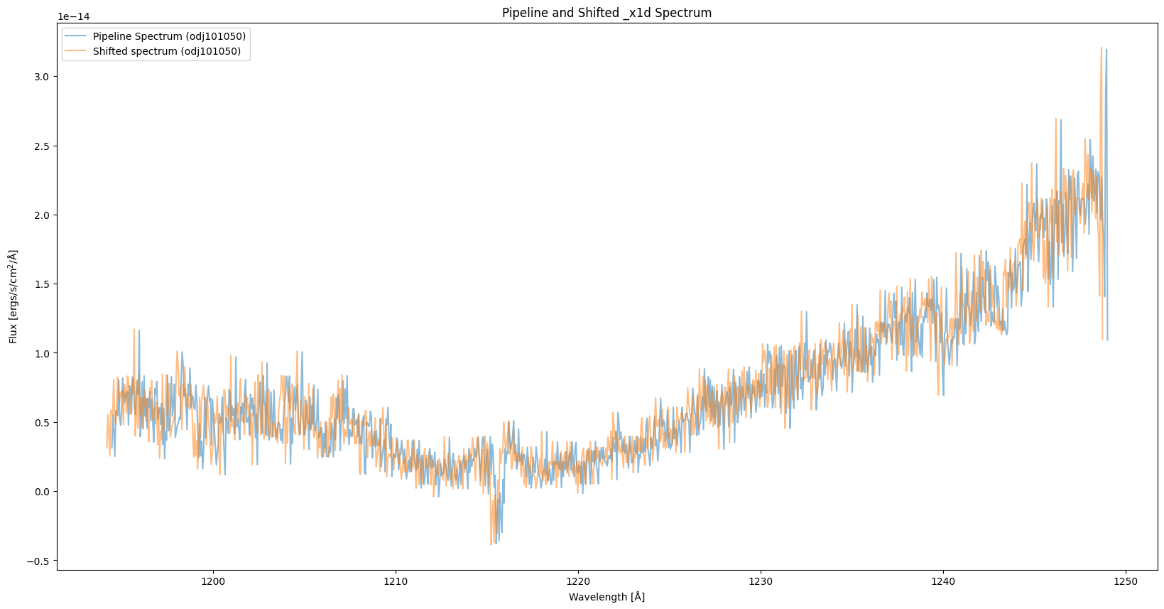
As seen in the plot, the spectrum is now shifted compared to the pipeline spectrum:

pip_x1d = os.path.join("./mastDownload/HST", "{}".format(target_id), "{}_x1d.fits".format(target_id))
shifted_x1d = Path("./Shifted/{}_x1d.fits".format(target_id))

with fits.open(pip_x1d) as hdu1, fits.open(shifted_x1d) as hdu2:
    pip_wl = hdu1[1].data["WAVELENGTH"][0]
    pip_flux = hdu1[1].data["FLUX"][0]
    
    shifted_wl = hdu2[1].data["WAVELENGTH"][0]
    shifted_flux = hdu2[1].data["FLUX"][0]

fig = plt.figure(figsize=(20, 10))
plt.plot(pip_wl, pip_flux, label="Pipeline Spectrum ({})".format(target_id), alpha=0.5)
plt.plot(shifted_wl, shifted_flux, label="Shifted spectrum ({})".format(target_id), alpha=0.5)
plt.legend(loc="best")
plt.xlabel("Wavelength [Å]")
plt.ylabel("Flux [ergs/s/cm$^2$/Å]")
plt.title("Pipeline and Shifted _x1d Spectrum")

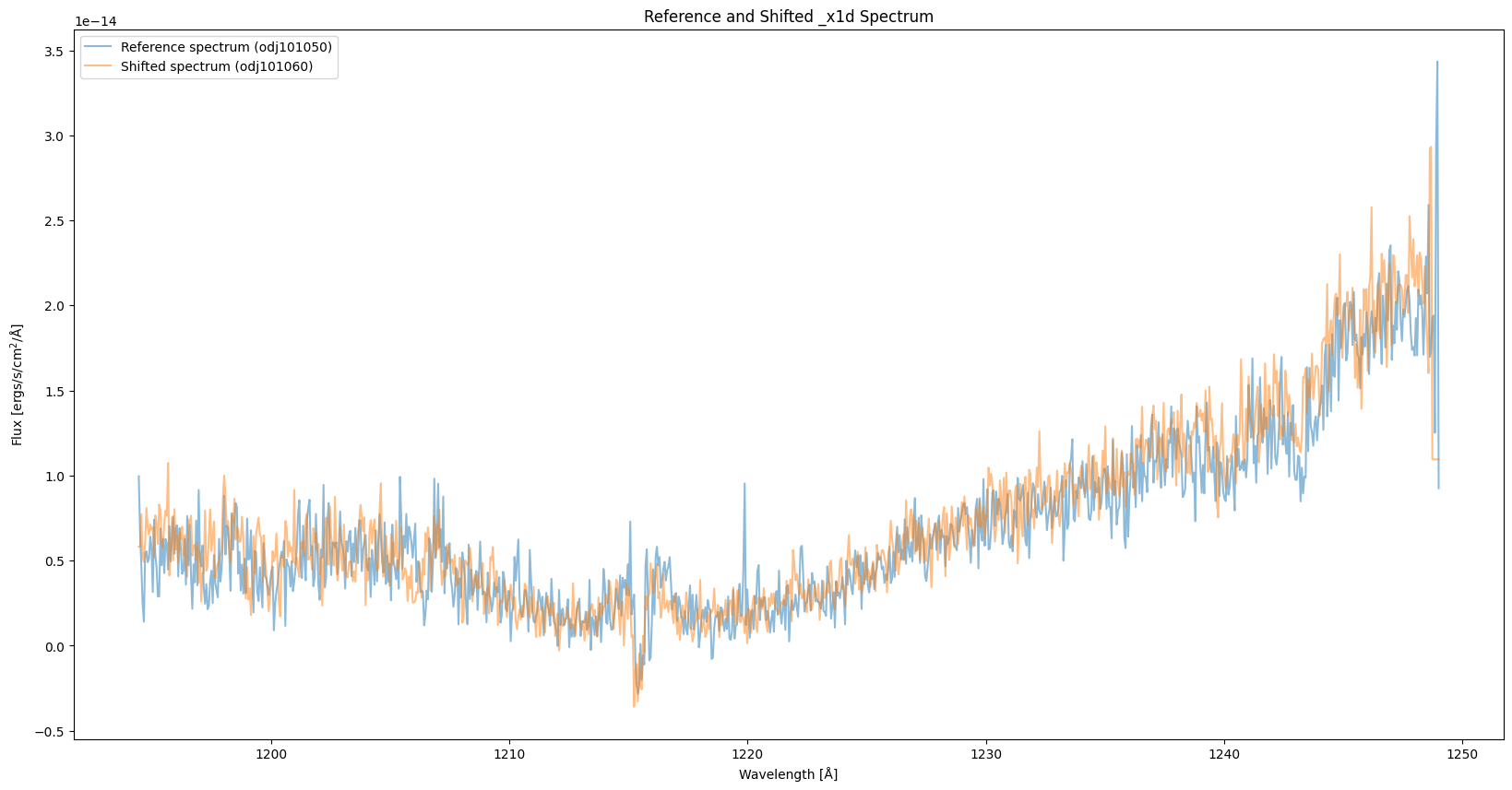
Spectrum Interpolation

Since the wavelength range of the pipeline and shifted spectra are different, we interpolate one of the spectra based on the wavelength of the other one so that the two spectra share the same wavelength array. As shown in the plot, the spectrum with “WAVECORR” turned off is systemetically shifted to the left.

ref_x1d = os.path.join("./mastDownload/HST", "{}".format(ref_id), "{}_x1d.fits".format(ref_id))

with fits.open(ref_x1d) as hdu1, fits.open(shifted_x1d) as hdu2:
    wl = hdu1[1].data["WAVELENGTH"][0]
    ref_flux = hdu1[1].data["FLUX"][0]
    
    shifted_wl = hdu2[1].data["WAVELENGTH"][0]
    shifted_flux = hdu2[1].data["FLUX"][0]
    
    shifted_flux = np.interp(wl, shifted_wl, shifted_flux)

fig = plt.figure(figsize=(20, 10))
plt.plot(wl, ref_flux, alpha=0.5, label="Reference spectrum ({})".format(target_id))
plt.plot(wl, shifted_flux, alpha=0.5, label="Shifted spectrum ({})".format(ref_id))
plt.legend(loc="best")
plt.xlabel("Wavelength [Å]")
plt.ylabel("Flux [ergs/s/cm$^2$/Å]")
plt.title("Reference and Shifted _x1d Spectrum")

Cross-Correlation

Dispersion per Pixel

To perform cross-correlation, detemine the shift amount in pixels, and then convert it into wavelength, we first need to determine the dispersion per pixel, i.e., the mean differences of adjacent data points in the wavelength grid.

mean_plate_scale = np.mean(wl[1:]-wl[:-1])
mean_plate_scale
print("The dispersion per pixel is {:.3f}".format(mean_plate_scale) + " Å/pixel")

Masking out the Lyman-alpha line

The absorption line at around 1215 Å is from Hydrogen Lyman-alpha, which mostly comes from the atmosphere and so should not shift like the science spectrum. Therefore, we need to mask out this region by separating the spectrum into two parts and perform two cross-correlations. There are other airglows lines in the ultraviolet that also does not shift with the science spectrum, including OI line at 1302 Å, OI line at 1305 Å, OI line at 1306 Å. For more information on the Airglow, see: AIRGLOW.

# the spectrum on the right of Lyman-alpha
ref_flux1 = ref_flux[wl > 1220]
shifted_flux1 = shifted_flux[wl > 1220]

# the spectrum on the left of Lyman-alpha
ref_flux2 = ref_flux[wl < 1213]
shifted_flux2 = shifted_flux[wl < 1213]

Lag and Cross-Correlation Coefficient

The lag is the displacement (in pixels) in the lagged spectrum. If the lag is 0, the spectra are aligned and not shifted.

The cross-correlation coefficient decodes how similar two spectra are. The cross-correlation coefficient takes values from -1 to 1: if it’s positive, the 2 spectra are positively correlated, if it’s negative, the 2 spectra are negatively correlated.

The cross-correlation algorithm shifts one of the input spectra according the the lags, and computes the cross-correlation coefficient for each lag. Then we take the lag with the maximum cross-coefficient and compute the corresponding displacement in wavelength space.

In general, the cross-correlation can be written as:

$C_{xy}[k]=\sum_n x[n] y[n+k]$

in which k is the lag, C is the cross-correlation coefficient, and x and y are the input spectra.

Normalization of the input spectra is required to ensure the cross-correlation coefficient is in the [-1,1] range.

def cross_correlate(shifted_flux, ref_flux):
    assert len(shifted_flux) == len(ref_flux), "Arrays must be same size"
    
    # Normalize inputs:
    shifted_flux = shifted_flux - shifted_flux.mean()
    shifted_flux /= shifted_flux.std()
    ref_flux = ref_flux - ref_flux.mean()
    ref_flux /= ref_flux.std()
    
    # centered at the median of len(a)
    lag = correlation_lags(len(shifted_flux), len(ref_flux), mode="same") 
    # find the cross-correlation coefficient
    cc = correlate(shifted_flux, ref_flux, mode="same") / float(len(ref_flux))
        
    return lag, cc

Polynimial Fitting and Zero Point Shift

After we get the lag and cross-correlation coefficient, we can determine the zero point shift by finding the lag with the maximum cross-correlation coefficient. However, since we only have discrete pixels shifts, we will fit a quadratic curve near the peak, get a fractional pixel shift, and find the maxima of the quadratic curve as the zero point shift. The zero point shift is shown as the green vertical line in the plot.

In this specific case, we choose the lag from -3 to 3, and fitted a 2 degree polynomial curve around the maximum cross-correlation coefficient to determine the shift in pixel space.The lag range and polynomial fitting is not the single solution that can be applied to all cases of wavelength zero point shifts. Users should experiment with the lag range and number of points to fit the polynomial curve based on the use case.

We first find the lag and cross-correlation coefficient of the right part of the spectrum:

fig = plt.figure(figsize=(10, 6))
lag, cc = cross_correlate(shifted_flux1, ref_flux1)
plt.plot(lag, cc, ".-", label="cross-correlation coefficient")

# fit quadratic near the peak to find the pixel shift
fitter = fitting.LinearLSQFitter()
# get the 5 points near the peak
width = 5
low, hi = np.argmax(cc) - width//2, np.argmax(cc) + width//2 + 1
fit = fitter(Polynomial1D(degree=2), x=lag[low:hi], y=cc[low:hi])
x_c = np.arange(-10, 0, 0.01)
plt.plot(x_c, fit(x_c), alpha=0.5, label="fitted quadratic curve")
# finding the maxima
shift1 = -fit.parameters[1] / (2. * fit.parameters[2])
plt.plot([shift1, shift1], [0, 1], alpha=0.5, label="quadratic curve maxima")

plt.xlim(-20, 20)
plt.ylim(0, 1)
plt.xlabel("Lag [pix]")
plt.ylabel("Cross-correlation coeff")
plt.title("15168-01, G140M/C1222 Observations")
plt.legend(loc="best")

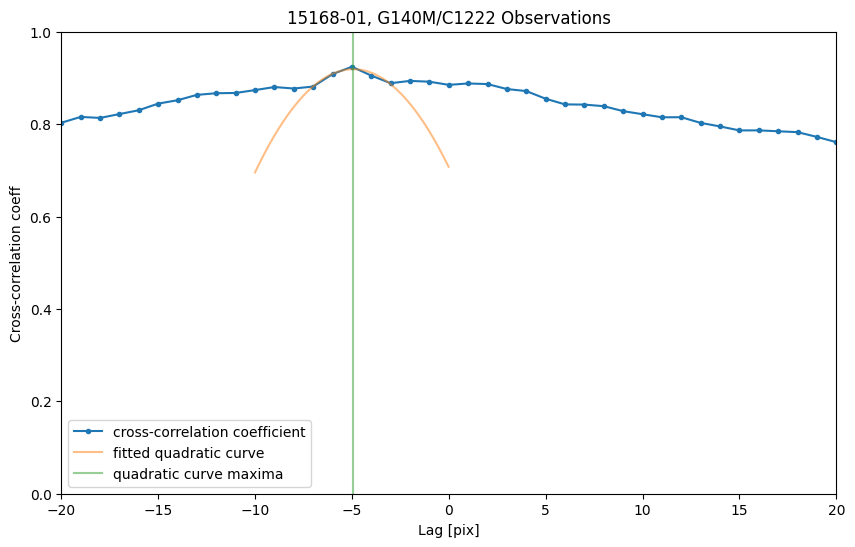
Convert the lag back into zero point shift in wavelength space:

print("Shift between the G140M/c1222 observations is {:.3f} pix = {:.3f}".format(shift1, shift1 * mean_plate_scale) + "Å")

Apply the same procedure to the left part of the spectrum:

fig = plt.figure(figsize=(10, 6))
lag, cc = cross_correlate(shifted_flux2, ref_flux2)
plt.plot(lag, cc, ".-", label="cross-correlation coefficient")

# fit quadratic near the peak to find the pixel shift
fitter = fitting.LinearLSQFitter()
# get the 5 points near the peak
width = 5
low, hi = np.argmax(cc) - width//2, np.argmax(cc) + width//2 + 1
fit = fitter(Polynomial1D(degree=2), x=lag[low:hi], y=cc[low:hi])
x_c = np.arange(-10, 0, 0.01)
plt.plot(x_c, fit(x_c), alpha=0.5, label="fitted quadratic curve")
# finding the maxima
shift2 = -fit.parameters[1] / (2. * fit.parameters[2])
plt.plot([shift2, shift2], [0, 1], alpha=0.5, label="quadratic curve maxima")

plt.xlim(-20, 20)
plt.ylim(0, 1)
plt.xlabel("Lag [pix]")
plt.ylabel("Cross-correlation coeff")
plt.title("15168-01, G140M/C1222 Observations")
plt.legend(loc="best")
print("shift2 between the G140M/c1222 observations is {:.3f} pix = {:.3f}".format(shift2, shift2 * mean_plate_scale) + "Å")

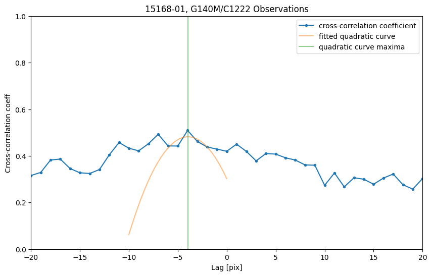
However, as shown in the plot, the maximum cross-correlation coefficient (~0.5) is relatively small, which suggests that the spectra are less similar on the left side. With such a small cross-correlation coefficient, we cannot determine a reasonable shift in the pixel space. Therefore, we only take the shift determined by the right part of the spectrum as the shift of the spectrum:

shift = shift1
print("shift between the G140M/c1222 observations is {:.3f} pix = {:.3f}".format(shift, shift * mean_plate_scale) + "Å")

Recalibrate Spectrum

After we determine the wavelength zero point shift, we can use the value to recalibrate the spectrum.

In the Calstis pipeline, “WAVECORR” calibration step determines the spectral shift values, and writes the keyword values SHIFTA1, SHIFTA2 for the spectral and spatial shifts, respectively, to the science header. To apply the spectral shift from the cross-correlation, we get the SHIFTA1, SHIFTA2 keywords from the _flt fits file, add the shift (in pixel space) to SHIFTA1, and write the updated keywords to the _raw fits file.

# get SHIFTA1, SHIFTA1 keywords from the first science extension
shifted_flt = Path("./Shifted/{}_flt.fits".format(target_id))
# since we have turned off WAVECOR at the beginning, SHIFTA1 should be 0
SHIFTA1 = fits.getval(shifted_flt, "SHIFTA1", 1)
SHIFTA2 = fits.getval(shifted_flt, "SHIFTA2", 1)
assert (SHIFTA1 == 0 and SHIFTA2 == 0)
# update SHIFTA1 (only in the spectral direction)
SHIFTA1 += shift
# update the the SHIFTA1, SHIFTA1 keywords in the _raw fits file first science extension
fits.setval(pip_raw, "SHIFTA1", value=SHIFTA1, ext=1)
fits.setval(pip_raw, "SHIFTA2", value=SHIFTA2, ext=1)

Then we need to turn the “WAVECORR” calibration switch to “omit” so that the Calstis calibration pipeline takes our new computed value instead of the wavecal returned value as the wavelength zero point shift.

fits.setval(pip_raw, "WAVECORR", value="OMIT", ext=0)
assert fits.getval(pip_raw, keyword="WAVECORR", ext=0) == "OMIT"

Recalibrate the spectrum using the Calstis pipeline. We create a new folder called “Recalibration” to store the recalibrated files. For more information on the Calstis pipeline, see: STIS Calibration, calstis.

# Create and clean "./Recalibration" directory for saving new files
if os.path.exists("./Recalibration"):
    shutil.rmtree("./Recalibration")
Path("./Recalibration").mkdir(exist_ok=True)
# Recalibration
res = stistools.calstis.calstis(pip_raw, verbose=False, outroot="./Recalibration/")
# calstis returns 0 if calibration completes; if not, raise assertion error
assert res == 0, f"CalSTIS exited with an error:  {res}"
recal_x1d = Path("./Recalibration/{}_x1d.fits".format(target_id))

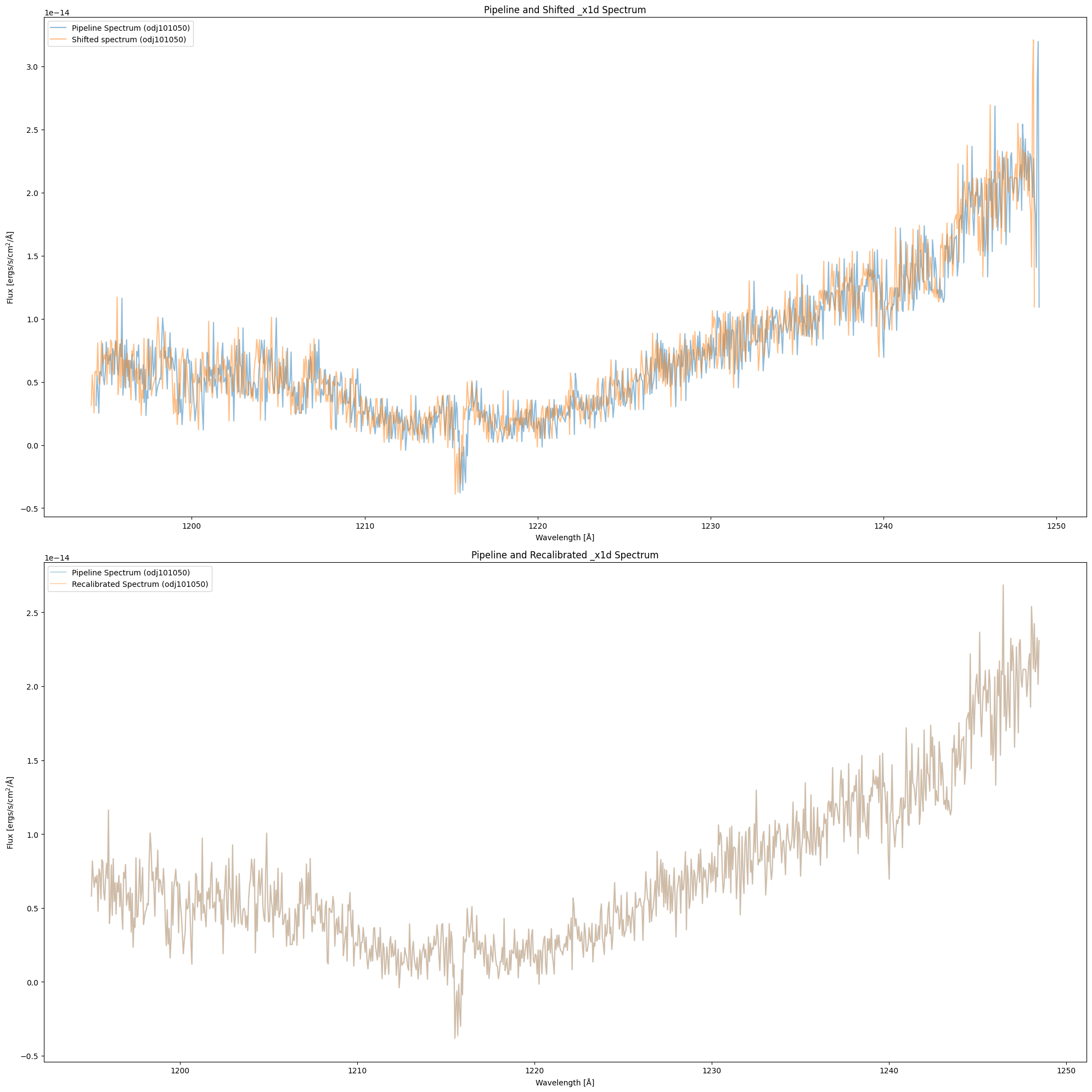
We compare the recalibrated spectrum with the pipeline spectrum. The top panel is the shifted spectrum (orange) and the pipeline spectrum (blue) of observation odj101050, which is the same as the plot in 2.1 Creating Shifted Spectrum. The bottom panel is the recalibrated spectrum (orange) and the pipeline spectrum (blue). The spectra almost overlap in the bottom panel, which suggests that the wavelength shift issue is solved in the recalibrated spectrum.

fig = plt.figure(figsize=(20, 20))
plt.subplot(2, 1, 1)
with fits.open(pip_x1d) as hdu1, fits.open(shifted_x1d) as hdu2:
    pip_wl = hdu1[1].data["WAVELENGTH"][0]
    pip_flux = hdu1[1].data["FLUX"][0]
    
    shifted_wl = hdu2[1].data["WAVELENGTH"][0]
    shifted_flux = hdu2[1].data["FLUX"][0]
    
plt.plot(pip_wl, pip_flux, label="Pipeline Spectrum ({})".format(target_id), alpha=0.5)
plt.plot(shifted_wl, shifted_flux, label="Shifted spectrum ({})".format(target_id), alpha=0.5)
plt.legend(loc="best")
plt.xlabel("Wavelength [Å]")
plt.ylabel("Flux [ergs/s/cm$^2$/Å]")
plt.title("Pipeline and Shifted _x1d Spectrum")

plt.subplot(2, 1, 2)
with fits.open(pip_x1d) as hdu1, fits.open(recal_x1d) as hdu2:
    wl1 = hdu1[1].data["WAVELENGTH"][0][10:-10]
    wl2 = hdu2[1].data["WAVELENGTH"][0][10:-10]
    
    flux1 = hdu1[1].data["FLUX"][0][10:-10]
    flux2 = hdu2[1].data["FLUX"][0][10:-10]
plt.plot(wl1, flux1, label="Pipeline Spectrum ({})".format(target_id), alpha=0.3)
plt.plot(wl2, flux2, label="Recalibrated Spectrum ({})".format(target_id), alpha=0.3)
plt.legend(loc="best")
plt.xlabel("Wavelength [Å]")
plt.ylabel("Flux [ergs/s/cm$^2$/Å]")
plt.title("Pipeline and Recalibrated _x1d Spectrum")
plt.tight_layout()

---

About this Notebook

Author: Keyi Ding

Updated On: 2023-04-14

This tutorial was generated to be in compliance with the STScI style guides and would like to cite the Jupyter guide in particular.

Citations

If you use astropy, matplotlib, astroquery, or numpy for published research, please cite the authors. Follow these links for more information about citations:

• Citing astropy/numpy/matplotlib

• Citing astroquery

---

Top of Page