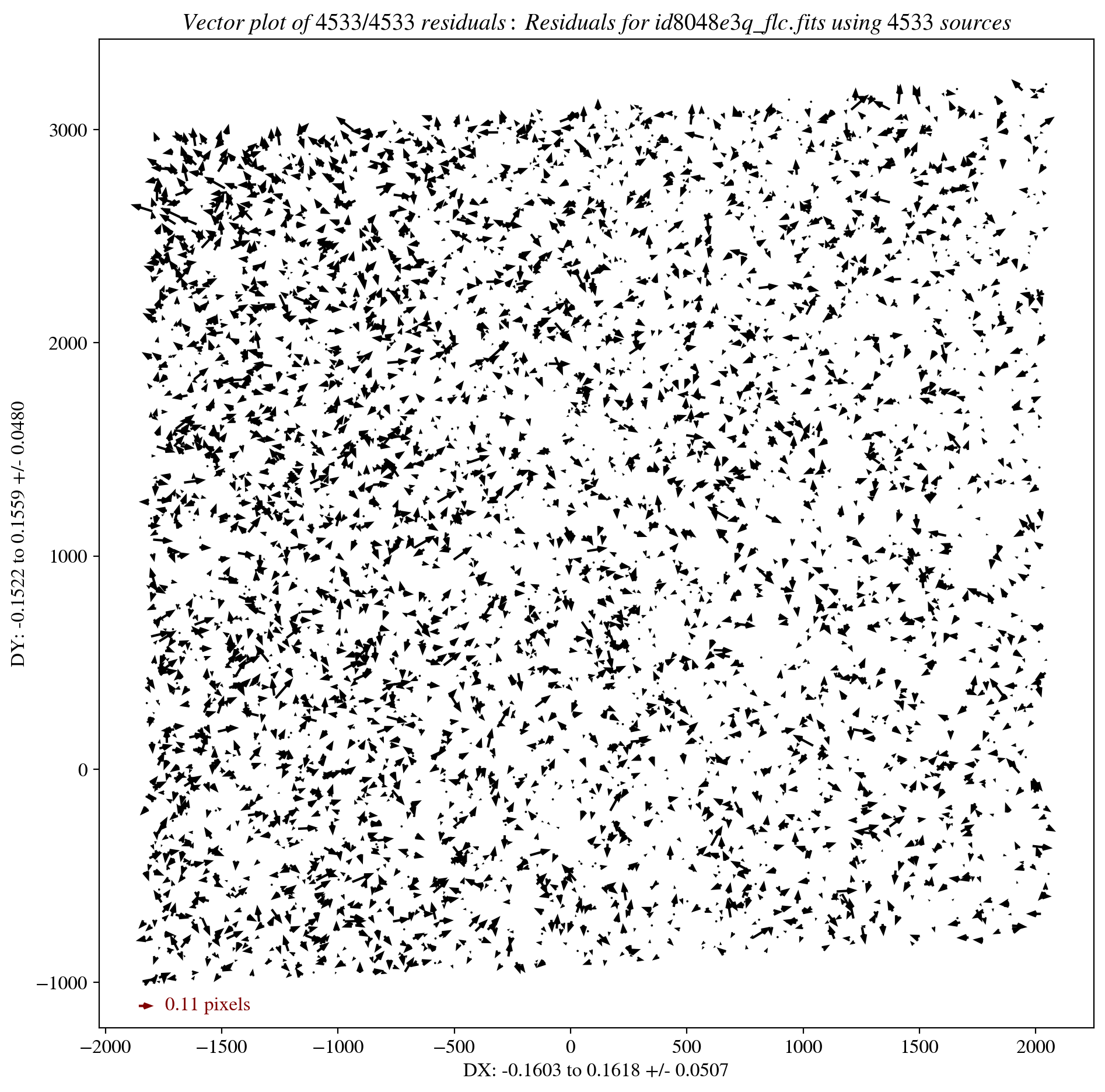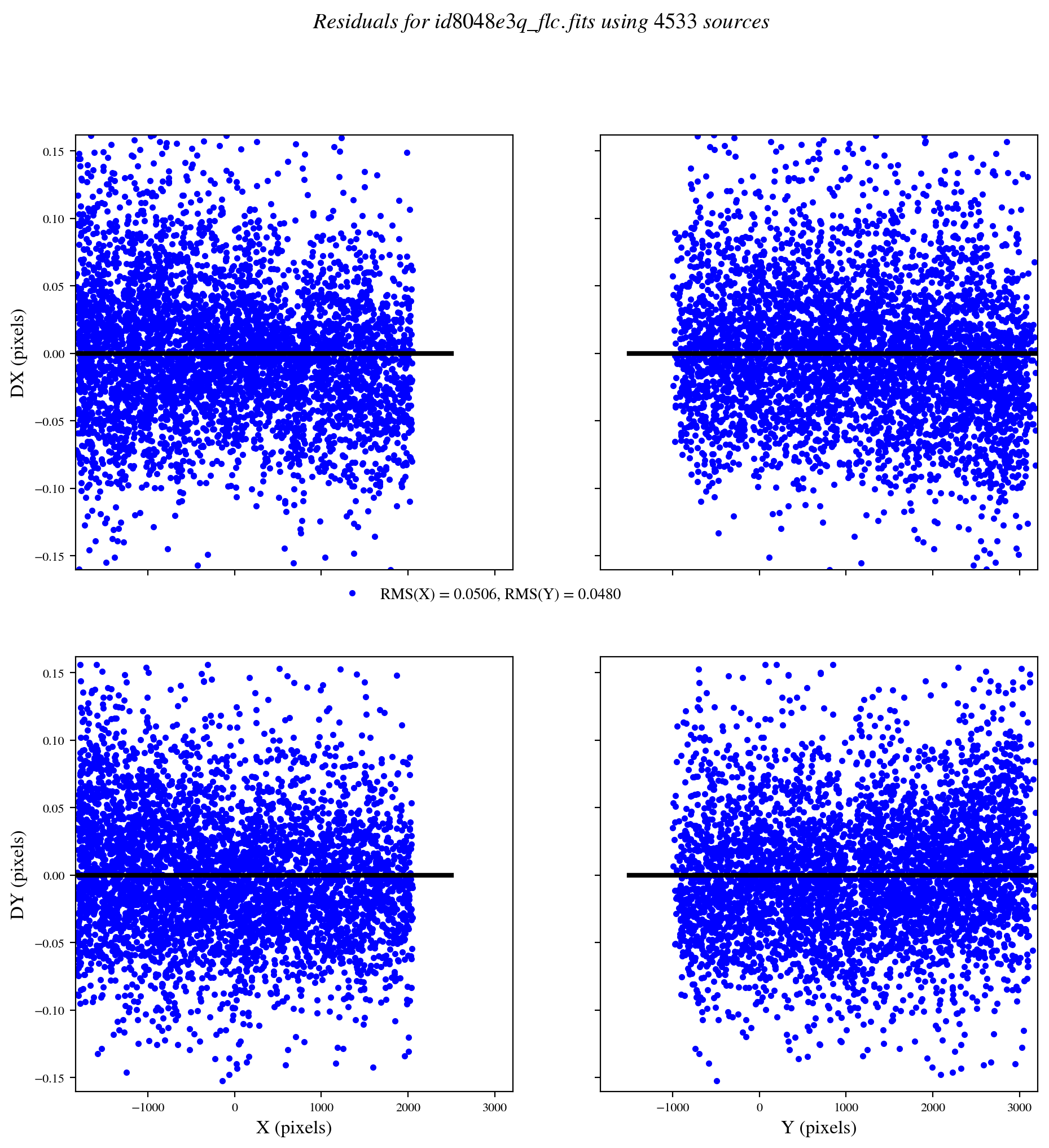
HST WFC3 Point Spread Function Modeling

---

Learning Goals

This notebook demonstrates how to create Point Spread Function (PSF) models for HST Wide Field Camera 3 (WFC3) observations.

The tutorial will allow users to complete the following tasks:

• Perform simple aperture photometry on science images for comparison with PSF photometry.

• Retrieve or create a PSF model for WFC3 single exposures (FLCs) and drizzled (DRZs) images.

• Complete basic science workflows including PSF photometry, subtraction, and decomposition.

Table of Contents

 Learning Goals
 1. Introduction
     1.1 Environment Setup
     1.2 Import Packages
     1.3 Download Data
     1.4 Aperture Photometry
 2. Exposure PSF Models
     2.1 Analytical PSF Models
     2.2 Empirical PSF Models
         2.2.1 Default Models
         2.2.2 Focus Perturbation
         2.2.3 Spatial Perturbation
     2.3 Stacked PSF Models
         2.3.1 Stellar Stacks
         2.3.2 MAST Stacks
 3. Drizzle PSF Models
     3.1 Create Drizzle
     3.2 Stack Stars
 Conclusions
 About this Notebook
     Additional Resources
     Software Citations

Acronyms:

• Point Spread Function (PSF)

• Hubble Space Telescope (HST)

• Wide Field Camera 3 (WFC3)

• WFC3 InfraRed detector (IR)

• WFC3 Ultraviolet and VISable detector (UVIS)

• Advanced Camera for Surveys (ACS)

• Wide Field and Planetary Camera 2 (WFPC2)

• Mikulski Archive for Space Telescopes (MAST)

• Flexible Image Transport System (FITS)

• Instrument Science Report (ISR)

• Full Width at Half Maximum (FWHM)

• Signal-to-Noise (S/N)

1. Introduction

Table of Contents

---

What is the Point Spread Function and why do we want to model it?

The purpose of a telescope is to collect, magnify, and record the intensity of light from astronomical sources. A telescope’s ability to resolve the size of objects is limited by its spatial resolution, which is determined by its aperture and the wavelength of light being observed, such that every telescope is fundamentally limited by the diffraction nature of light. The minimum size of an image that the light can be focused onto is known as the Airy disk. In addition, the shape of the image will be altered by any optical aberrations in the telescope’s system of mirrors, lenses, filters, and camera detectors. When observing unresolved point sources such as stars, these factors determine the size and shape of the focused image. This distribution of light as a function of position on the telescopes detectors is known as the Point Spread Function (PSF). More simply, the PSF describes how the light from an unresolved source is distributed across multiple pixels when it is recorded by the telescope’s camera.

While a well-focused telescope produces a very small image of point sources, the shape will be distorted and the light is effectively scattered to an infinite radius. Therefore, a model of the PSF is required to accurately measure astrometry (positions) and photometry (brightnesses) of objects in astronomical images. In the case of the HST WFC3 this is especially important because the images are undersampled, which means the telescope is capable of delivering higher resolution than the detector pixels can record. The PSF will vary depending on the telescopes focus, and also significantly with location on the WFC3 detector due to optical distortions in the light path that are designed to minimize light loss by reducing the number of optical reflections. For these reasons, the WFC3 team has produced a library of PSF models and tools for users on the WFC3 PSF webpage.

Finally, astrometric and photometric measurements can generally be made either from individual calibrated exposures known as FLTs and FLCs for WFC3, or exposures that are combined into a mosaic through drizzling. In theory, modeling individual exposures is always preferable because these images are on the telescope’s intrinsic pixel grid without any modification. However, this requires bright unresolved sources that have been observed with a relatively short exposure time, so that images are not strongly affected by cosmic rays. In addition, many astronomical sources are very faint, requiring a combination of multiple dithered exposures to obtain sufficient signal-to-noise (S/N) for analysis. For these reasons, we will demonstrate techniques for constructing PSF models for both individual calibrated exposures and drizzled mosaics.

Users looking for a fundamental introduction to aperture photometry and PSF photometry may find this excellent series of video tutorials by Boyce-Astro helpful, as well as this description of the Airy Disk by Edmund Optics. In addition, detailed information on WFC3 can be found on the WFC3 Website, WFC3 PSF Webpage, WFC3 Instrument Handbook, and WFC3 Data Handbook. In addition, the publication by Anderson & King 2000 provides information about the effects of undersampling on the HST PSF. Finally, we note that the flux measured for each source will depend on the radial extent of the PSF model. Specifically, models truncated at a given radius will encompass a fraction of the total electrons from each star, which can be accounted for by using an encircled energy ratio correction. See Section 9.1.8 of the WFC3 Data Handbook, WFC3 ISR 2022-02, and the WFC3 UVIS and IR encircled energy webpages for more information.

We hope this notebook provides valuable information and examples for constructing HST WFC3 PSF models. While the focus in this notebook is for the WFC3 instrument, the majority of the code also applies to HST Advanced Camera for Surveys (ACS) observations, as well as archival Wide Field and Planetary Camera 2 (WFPC2) observations. See ACS ISR 2006-01 for more information on the ACS PSF models. Finally, users may find several helpful resources on the WFC3 Software webpage.

1.1 Environment Setup

Table of Contents

---

This Jupyter Notebook requires users to install the stenv Python environment maintained by STScI.

Detailed installation instructions can be found on the stenv readthedocs. For completeness, the terminal commands for MacOS with ARM chips are included below:

conda update conda conda env create –name stenv2024 –file https://github.com/spacetelescope/stenv/releases/download/2024.02.05/stenv-macOS-ARM64-py3.11-2024.02.05.yaml conda activate stenv2024 conda install -c conda-forge gfortran conda clean -t jupyter lab

NOTE: The following non-Python tools are needed to run some advanced features of the Jupyter Notebook. Specifically, a FORTRAN compiler and the hst1pass code are only required for PSF perturbation with individual exposures (FLCs). These tools are not required for stacking stars or creating PSF models for drizzled images (DRZs). The code will automatically compile hst1pass. If this step encounters errors, then manual instructions for installing FORTRAN and hst1pass are included below:

• hst1pass - FORTRAN code for performing photometry and PSF perturbation as documented in WFC3 ISR 2022-05.

FORTRAN can be installed by typing the command conda install -c conda-forge gfortran into a terminal. If the installation is successful, then typing gfortran --version should return a message similar to the following: GNU Fortran (GCC) 13.2.0 Copyright (C) 2023 Free Software Foundation, Inc..

Next, to install hst1pass proceed to https://www.stsci.edu/~jayander/HST1PASS/CODE/hst1pass/ and download the latest version of hst1pass.F, e.g. hst1pass.2023.11.07_v1f.F, or use the version in this notebook’s repository. Save this to your computer and compile the code using the command: gfortran hst1pass.2023.11.07_v1f.F -o hst1pass.e.

1.2 Import Packages

Table of Contents

---

The following Python packages are required to run the Jupyter Notebook:

• os - change and make directories

• glob - gather lists of filenames

• shutil - copy files between folders

• tarfile - read and write compressed tar files

• urllib - download files hosted online

• ipython - cell formatting and interactives

  • display.clear_output - clear text from cells

• numpy - math and array functions

  • percentile - lognorm percentile clipping

• matplotlib - create graphics

  • pyplot - make figures and graphics

  • colors.LogNorm - display image normalization

  • patches.Rectangle - overlay rectangular regions

• astroquery - download astronomical data

  • mast.Observations - query MAST database

• astropy - model fitting and file handling

  • io.fits - import FITS files

  • table.QTable - tables with physical units

  • modeling.models - Gaussian and Moffat models

  • modeling.fitting - fitting methods for models

  • visualization.simple_norm - display image normalization

  • stats.sigma_clipped_stats - mean, median, and standard deviation

  • stats.SigmaClip - sigma-clip provided data

• photutils - aperture and PSF photometry tools

  • detection.DAOStarFinder - finding stars in images

  • detection.find_peaks - finding peaks in images

  • photutils.centroids - finding stellar centroids

  • photutils.aperture - aperture photometry tools

    • aperture_photometry - measure aperture photometry

    • CircularAperture - measure photometry in circle

    • CircularAnnulus - measure photometry in annulus

    • ApertureStats - calculate aperture statistics

  • photutils.psf - PSF photometry tools

    • PSFPhotometry - perform PSF photometry

    • SourceGrouper - group sources for fitting

    • IntegratedGaussianPRF - Gaussian model for PSF fitter

    • GriddedPSFModel - enables spatially-dependent PSF grids

    • STDPSFGrid - reads STScI standard PSF models into a grid

    • stdpsf_reader - reads STScI standard PSF format models

    • FittableImageModel - convert stacked stars to fitable model

• scipy - mathematical interpolation and shift functions

  • ndimage.shift - fractional array shifts

• drizzlepac - combine HST images into mosaics

  • astrodrizzle - combine exposures by drizzling

  • tweakreg - align exposures to a common WCS

import os
import glob
import shutil
import tarfile
from IPython.display import clear_output
import numpy as np
import matplotlib.pyplot as plt
from matplotlib.colors import LogNorm
from matplotlib.patches import Rectangle
from astroquery.mast import Observations
from astropy.io import fits
from astropy.table import Table, QTable
from astropy.visualization import simple_norm
from astropy.stats import sigma_clipped_stats, SigmaClip
from photutils.detection import DAOStarFinder
from photutils.aperture import (ApertureStats, CircularAnnulus,
                                CircularAperture, aperture_photometry)
from photutils.psf import (FittableImageModel, GriddedPSFModel, IntegratedGaussianPRF, 
                           PSFPhotometry, SourceGrouper, STDPSFGrid)
from drizzlepac import tweakreg, astrodrizzle

# Custom functions written in psf_utilities.py.
# Contains functions for making various figures and maniputlating science images.
from psf_utilities import save_figure, setup_matplotlib, create_mask, plot_apertures, \
    plot_psf_results, download_psf_model, make_cutouts, stack_cutouts, plot_cutout_grid

# Custom functions written in mast_api_psf.py.
# Contains functions for downloading image cutouts from the MAST PSF library server.
import mast_api_psf

The following task in the stsci.skypac package can be run with TEAL:
                                    skymatch                                    

The following tasks in the drizzlepac package can be run with TEAL:
    astrodrizzle       config_testbed      imagefindpars           mapreg       
       photeq            pixreplace           pixtopix            pixtosky      
  refimagefindpars       resetbits          runastrodriz          skytopix      
     tweakback            tweakreg           updatenpol

Note that we can access the helpful documentation string for any of the custom-defined functions using help(). For example:

help(save_figure)

Help on function save_figure in module psf_utilities:

save_figure(figure, filename, show_figure)
    Save the current figure and display or close the file.
    There are no returns, the filepath is simply printed.
    
    Parameters
    ----------
    figure : matplotlib.figure.Figure
        The matplotlib image that the user would like to save.
    filename : str
        The full filepath including the desired filename to save.
    show_figure : bool
        The figure will be shown in the notebook if set to True.

Set the main code, data, PSF, plot, AstroDrizzle, and TweakReg directories. Set the backend configuration to ‘retina’, which improves the resolution of figures in notebooks.

code_dir = os.getcwd()+'/'
data_dir = code_dir+'data/'
psfs_dir = code_dir+'psfs/'
plot_dir = code_dir+'plot/'
driz_dir = code_dir+'driz/'
tweak_dir = code_dir+'tweak/'

os.chdir(code_dir)

print('\nThe code_dir is:', code_dir)

for folder in ['data', 'psfs', 'plot', 'driz', 'tweak']:
    if not os.path.exists(folder):
        os.mkdir(folder)
    else:
        print(f'{folder} directory exists.')

%config InlineBackend.figure_format = 'retina'

The code_dir is: /home/runner/work/hst_notebooks/hst_notebooks/notebooks/WFC3/point_spread_function/

1.3 Download Data

Table of Contents

---

In this example, we will be using HST WFC3 imaging of the globular cluster Omega Centauri (NGC 5139). Specifically, utilizing exposures that are not centered on the cluster core so there is a moderate density of bright stars. This source was chosen because it serves as a frequent target for both science and calibration exposures, and has been observed with every UVIS and IR filter onboard WFC3. A complete list of WFC3 filters is available in the Data Handbook for the UVIS and IR channels. First, we use astroquery to retrieve the calibrated exposure from MAST.

hst_wfc3_f606w_file = 'id8048dyq_flc.fits'

Observations.download_file('mast:HST/product/'+hst_wfc3_f606w_file, local_path=data_dir+hst_wfc3_f606w_file, cache=True)

Downloading URL https://mast.stsci.edu/api/v0.1/Download/file?uri=mast:HST/product/id8048dyq_flc.fits to /home/runner/work/hst_notebooks/hst_notebooks/notebooks/WFC3/point_spread_function/data/id8048dyq_flc.fits ...

 [Done]

('COMPLETE', None, None)

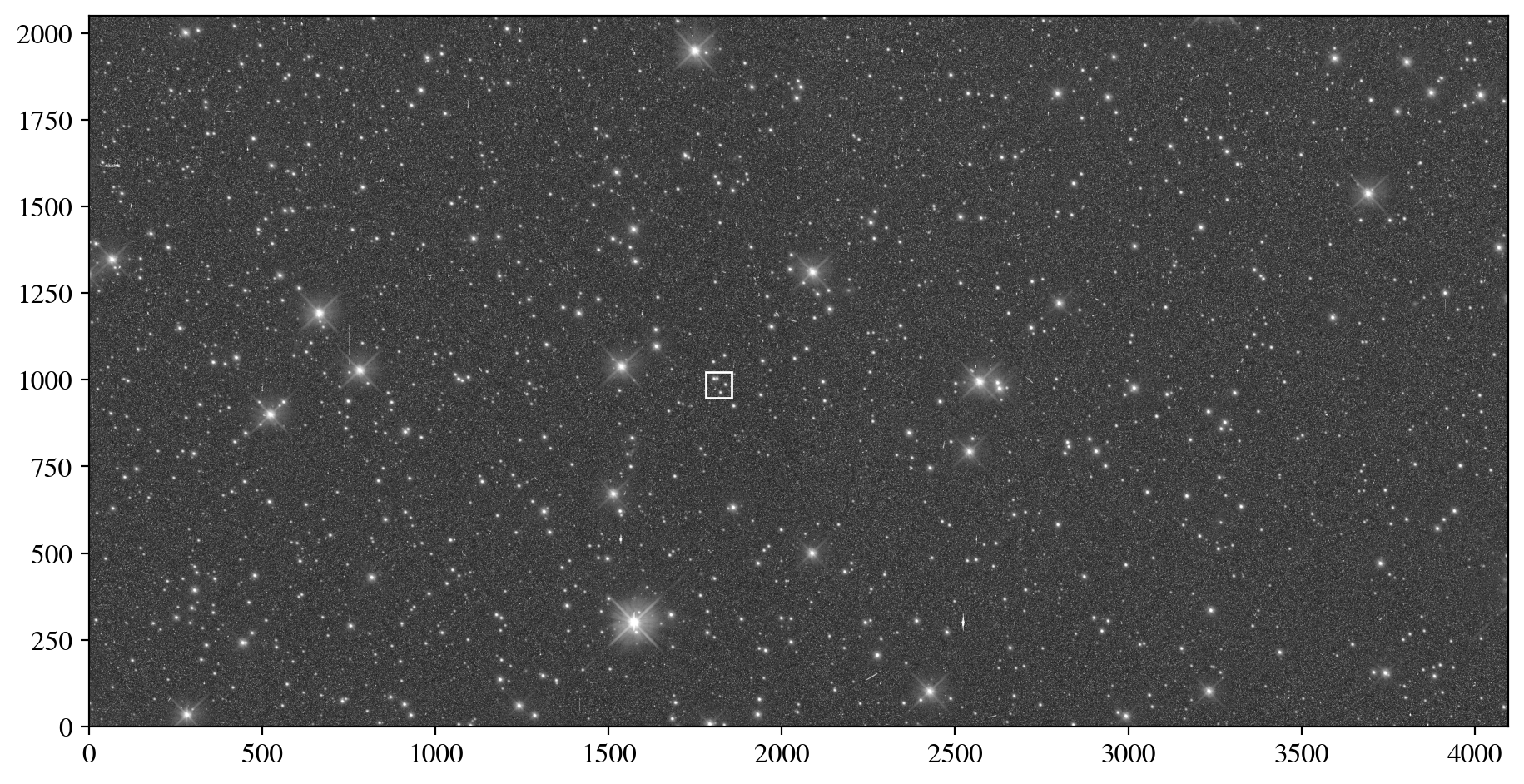
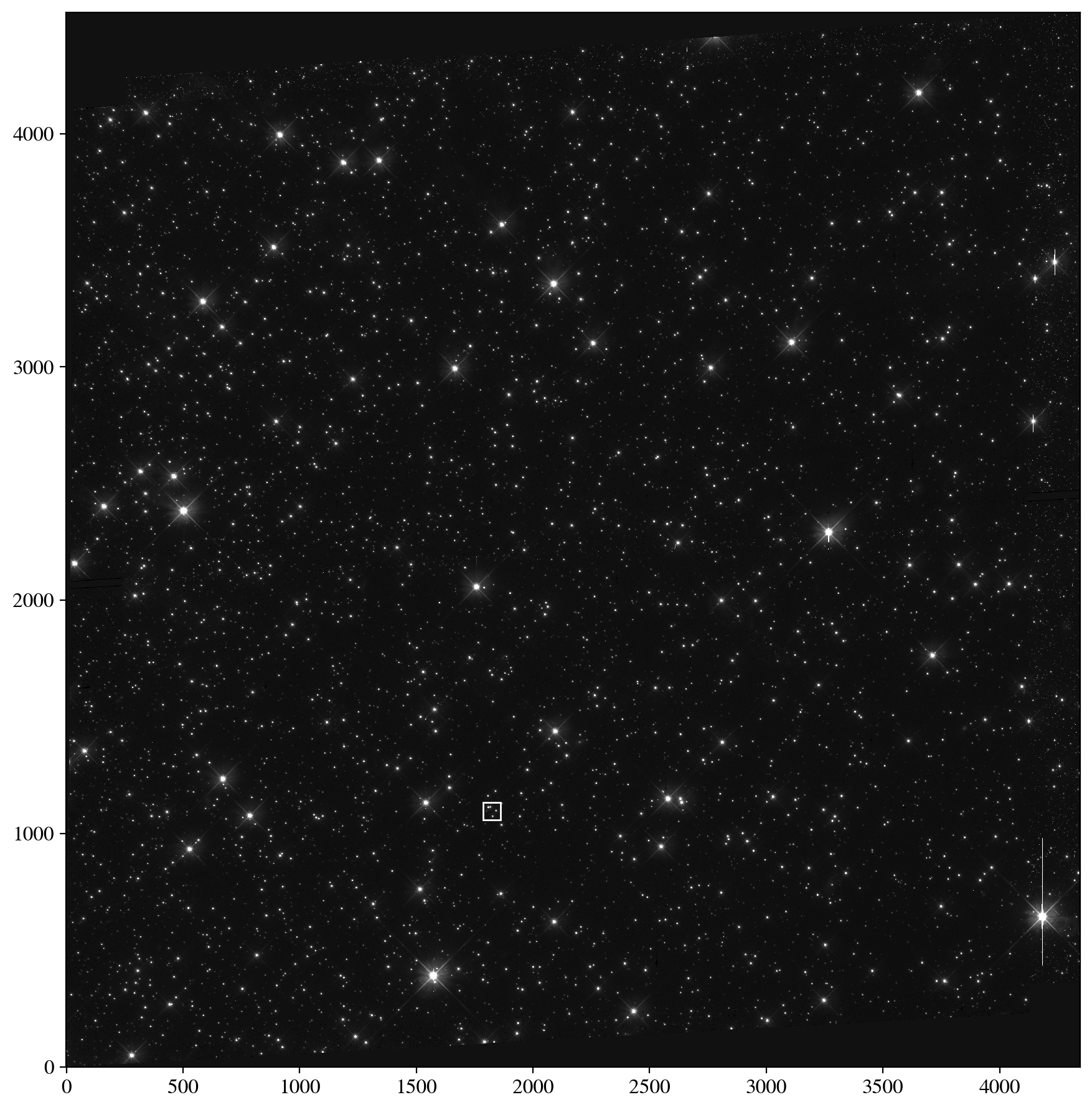
Next, let’s display the image of Omega Centauri and add a rectangle showing the region of the image that we will focus on in this analysis. We select a small region of the image that contains isolated and blended stars to highlight key concepts in aperture and PSF photometry. The WFC3/UVIS pixel scale is 0.03962 arcseconds per pixel so selecting a region of 75 pixels corresponds to approximately 3 arcseconds. The UVIS detector has two chips that can be accessed in the FITS files from extensions ['SCI', 1] for UVIS2 and ['SCI', 2] for UVIS1. The lower-left corner of the detector is the location (0, 0) pixels, so we use the origin = 'lower' option. Finally, we display the image on a logarithmic scale to view both very faint and bright stars simultaneously.

with fits.open(data_dir+hst_wfc3_f606w_file) as hdul:
    sci_data = hdul['SCI', 1].data
print('The image dimensions are:', np.shape(sci_data))

my_figure_size, my_fontsize = setup_matplotlib('notebook', 1.2)
figure, axes = plt.subplots(1, 1, figsize=my_figure_size)
cutout_size = 75 # 75 WFC3 UVIS pixels = 3 arcseconds.

axes.add_patch(Rectangle((1818-cutout_size/2, 986-cutout_size/2), width=cutout_size, height=cutout_size, fill=None, color='w'))
norm = LogNorm(vmin=np.percentile(sci_data, 10.0), vmax=np.percentile(sci_data, 99.9))
axes.imshow(sci_data, cmap='gray', origin='lower', aspect='equal', norm=norm)
plt.show()

The image dimensions are: (2051, 4096)

1.4 Aperture Photometry

Table of Contents

---

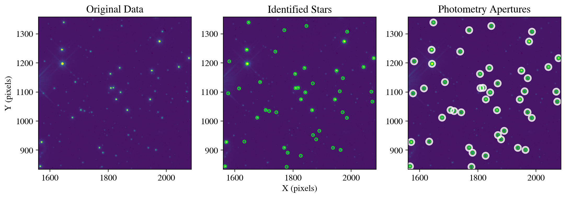
First, we can perform simple aperture photometry on the image. This consists of detecting stars in the image, assigning them an aperture within which to measure the enclosed flux, and creating a background annulus that is used to subtract the background level. In ground-based astronomy this is commonly referred to as the “sky” level. In this example, we create a mask so that we only find and measure the properties of stars that are within our selected box region.

The cell below first calculates the mean, median, and standard deviation for the background, initializes the star finder function with a threshold of 500 electrons and a FWHM of three pixels, and then creates a mask so that the star finding algorithm will only search within our zoomed-in box region. Next, the DAOStarFinder function searches for peaks and returns a list of sources. We then assign to the position of each source a circular annulus designed to measure the flux of the star, and a background annulus that measures the local background flux.

mean, median, std = sigma_clipped_stats(sci_data, sigma=3.0)
daofind = DAOStarFinder(threshold=500, fwhm=3.0, roundhi=0.5)
mask = create_mask(sci_data, cutout_size, 1818, 986)
sources = daofind(sci_data - median, mask=mask)
positions = np.transpose((sources['xcentroid'], sources['ycentroid']))
apertures_stellar = CircularAperture(positions, r=5.0)
apertures_annulus = CircularAnnulus(positions, r_in=9, r_out=12)
phot_table = aperture_photometry(sci_data, apertures_stellar)

Next, we use the aperture and annulus measurement for each star to calculate the sigma-clipped background flux, and subtract it to obtain only the flux of each star.

aperture_stats = ApertureStats(sci_data, apertures_stellar, sigma_clip=None)
background_stats = ApertureStats(sci_data, apertures_annulus, sigma_clip=SigmaClip(sigma=3.0, maxiters=10))
total_background = background_stats.median * aperture_stats.sum_aper_area.value # area of annulus.
flux_background_sub = aperture_stats.sum - total_background
phot_table['total_background'] = total_background
phot_table['flux_background_sub'] = flux_background_sub

for col in phot_table.colnames:  
    if col not in ('id', 'npix'):
        phot_table[col].info.format = '%.2f'

Finally, we display the flux measurements in a table and create a figure showing the science data, stellar apertures (green circles) and background annuli (white circles).

print('\n', phot_table, '\n')

plot_apertures(data=sci_data, 
               xcenter=1818, 
               ycenter=986, 
               cutout_size=cutout_size, 
               apertures_stellar=apertures_stellar, 
               apertures_annulus=apertures_annulus)

save_figure(figure, plot_dir+'fig1_aperture_photometry.pdf', True)

  id xcenter ycenter aperture_sum total_background flux_background_sub
      pix     pix                                                    
--- ------- ------- ------------ ---------------- -------------------
  1 1822.05  963.68     33720.33           989.01            32731.32
  2 1836.63  986.73     32338.86           970.57            31368.29
  3 1803.54 1003.36     63426.72          1303.54            62123.18
  4 1812.01 1004.03     34106.74          1261.96            32844.78 

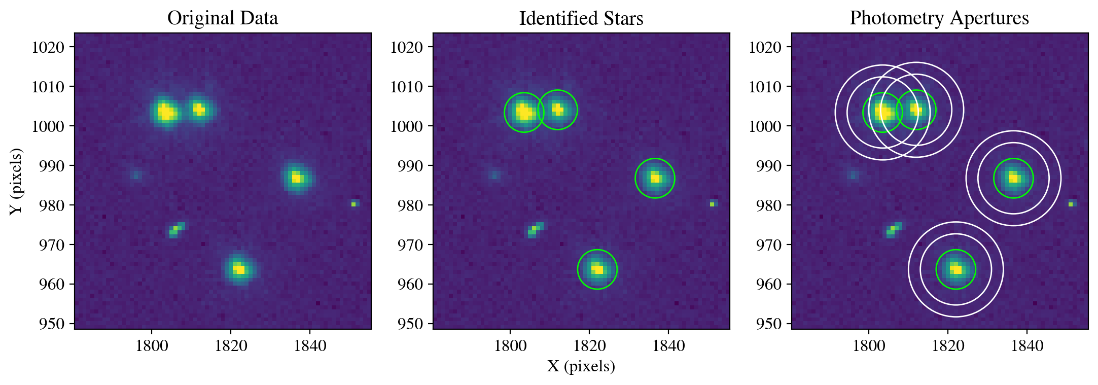
Figure saved as: /home/runner/work/hst_notebooks/hst_notebooks/notebooks/WFC3/point_spread_function/plot/fig1_aperture_photometry.pdf

2. Exposure PSF Models

Table of Contents

---

As described in the Introduction, we may perform PSF modeling, photometry, and astrometry on either individual exposures or mosaics that combine exposures through drizzling. The sections below contain several different workflows with various options depending on your science goals and the available data. The flowchart below is meant as a general guide for deciding which sections are most relevant for your project. We highlight that several different paths may be applicable to a single dataset and users are encouraged to experiment with the options below.

NOTE: Users that are creating PSF models for drizzled images and not single exposures can proceed to the section on Drizzle PSF Models.

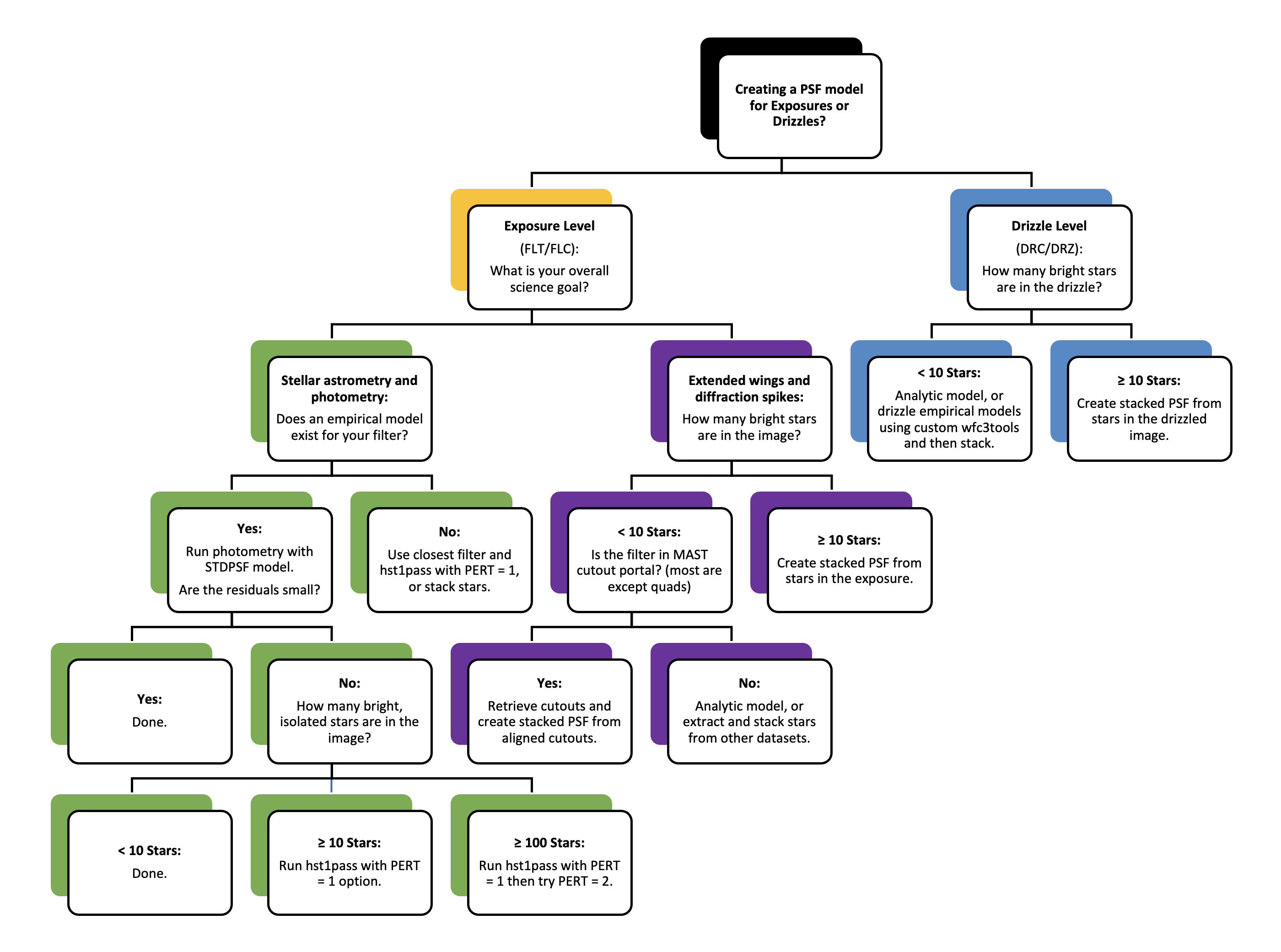
Note that the left fork under the drizzle level branch is an advanced workflow that involves drizzling the empirical models provided by the WFC3 team into FLC files. This requires installing the wfc3_photometry package, running the make_model_star_image() function within PSFUtils.py, and then stacking the drizzled models. This functionality is under development and not yet officially supported.

2.1 Analytical PSF Models

Table of Contents

---

The example above demonstrates how to perform basic aperture photometry of sources. However, we can see that two of the stars overlap in the image and their fluxes are blended. Therefore, aperture photometry cannot be used reliably for crowded fields, and requires corrections when using multiple filters as the apertures do not account for changing resolution with wavelength. Without any knowledge of the intrinsic shape of the PSF, we can first fit purely analytical functions such as a Gaussian, Moffat, Lorentzian, or Voigt profile to each star. While the majority of our functions are specified in the psf_utilities.py module, we explicitly define two common photometry functions here so users can easily experiment and change common options depending on their data and goals.

Critically, we note that the size of the fit_shape variable (in pixels) determines the number of pixels used to constrain the fit. If the value is small, the core pixels of the source will dominate the fit, while larger values will weight more wing emission when determining the best fit model.

def calculate_photometry(sci_data, sources, psf_model):
    
    """
    A function that performs PSF photometry given a science image, 
    a list of sources, and a PSF model in the PSFPhotometry format. 
    See the photutils documentation below for additional examples:
    
    https://photutils.readthedocs.io/en/stable/psf.html

    Parameters
    ----------
    sci_data : np.ndarray
        The np.ndarray containing the array of science data.
    sources : astropy.table.table.QTable
        The astropy table of sources from the daofind function.
    psf_model : photutils.psf.GriddedPSFModel
        An astropy compatible model PSF or grid of PSFs.

    Returns
    -------
    phot : astropy.table.table.QTable
        An astropy quantity table with measured source photometry.
    psfphot : photutils.psf.PSFPhotometry
        Contains results of PSF fitting for use with other functions.
    """

    # Perform PSF fitting using an 9x9 pixel region.    
    fit_shape = (9, 9)
    grouper = SourceGrouper(min_separation=20)
    finder = DAOStarFinder(threshold=500, fwhm=3.0, roundhi=0.5)
    psfphot = PSFPhotometry(psf_model, fit_shape, finder=finder, aperture_radius=5, grouper=grouper)
    
    init_params = QTable()
    init_params['x'] = sources['xcentroid']
    init_params['y'] = sources['ycentroid']
    phot = psfphot(sci_data, init_params=init_params)
    phot['x_fit'].info.format = '.2f'
    phot['y_fit'].info.format = '.2f'
    phot['flux_fit'].info.format = '.2f'
    phot['qfit'].info.format = '.3f'
    print('\033[1m'+'\nPSF Photometry (before subtraction):\n'+'\033[0m')
    print(phot[('id', 'x_fit', 'y_fit', 'flux_fit', 'qfit')])
    print('')
    
    return phot, psfphot

def calculate_residuals(resid, sources):
    
    """
    A function that calculates the residual flux at the 
    locations of stars in a given PSF-subtracted image.

    Parameters
    ----------
    resid : np.ndarray
        A residual image created by psfphot.make_residual_image().
    sources : astropy.table.table.QTable
        The astropy table of sources from the daofind function.

    Returns
    -------
    phot_table : astropy.table.table.QTable
        Prints an astropy table with measured source photometry.
    """

    # Use the PSF fitting residuals to calculate remaining fluxes.
    phot_table = aperture_photometry(resid, apertures_stellar)
    aperture_stats = ApertureStats(resid, apertures_stellar, sigma_clip=None)
    background_stats = ApertureStats(resid, apertures_annulus, sigma_clip=SigmaClip(sigma=3.0, maxiters=10))
    total_background = background_stats.median * aperture_stats.sum_aper_area.value # area of annulus.
    flux_background_sub = aperture_stats.sum - total_background
    phot_table['total_background'] = total_background
    phot_table['flux_background_sub'] = flux_background_sub
    
    for col in phot_table.colnames:  
        if col not in ('id', 'npix'):
            phot_table[col].info.format = '%.2f'

    print('\033[1m'+'\nAperture Photometry (after subtraction):\n'+'\033[0m')
    
    return print(phot_table, '\n')

In this first analytical example, we fit Gaussian profiles to the four stars in our subimage and display the data, model, and residuals. We provide an initial guess for the width (sigma) using an approximate full width at half maximum (FWHM) of 2 pixels, where \(\sigma\) = FWHM/2.355. Users are encouraged to experiment with this value to see how the resulting fit and residuals change. First, the calculate_photometry function uses the provided PSF model with the photutils PSFPhotometry function to fit the model to the stars. In essence, the flux of the normalized PSF model is scaled up to match the flux of each star. In this case, neighboring stars are fit simultaneously. The make_residual_image function then subtracts the best fit model so the flux residuals can be examined. Finally, we call the calculate_residuals function with the exact same stellar and background photometry apertures used in Section 1.4 in order to measure the residual fluxes. A smaller residual flux generally implies a better fit, but the residuals should be inspected as over and undersubtractions from different portions of the star can also yield a small net residual flux.

psf_model = IntegratedGaussianPRF(flux=1000, sigma=2.0/2.355)
photometry, psfphot = calculate_photometry(sci_data, sources, psf_model)
resid = psfphot.make_residual_image(sci_data, (19, 19))
figure = plot_psf_results(sci_data, resid, 1818, 986, cutout_size)
save_figure(figure, plot_dir+'fig2_gaussian_model.pdf', True)
calculate_residuals(resid, sources)

PSF Photometry (before subtraction):

 id  x_fit   y_fit  flux_fit  qfit
--- ------- ------- -------- -----
  1 1822.08  963.70 20494.30 0.748
  2 1836.70  986.77 19707.67 0.735
  3 1803.57 1003.38 38284.30 0.734
  4 1812.03 1004.04 19589.59 0.848

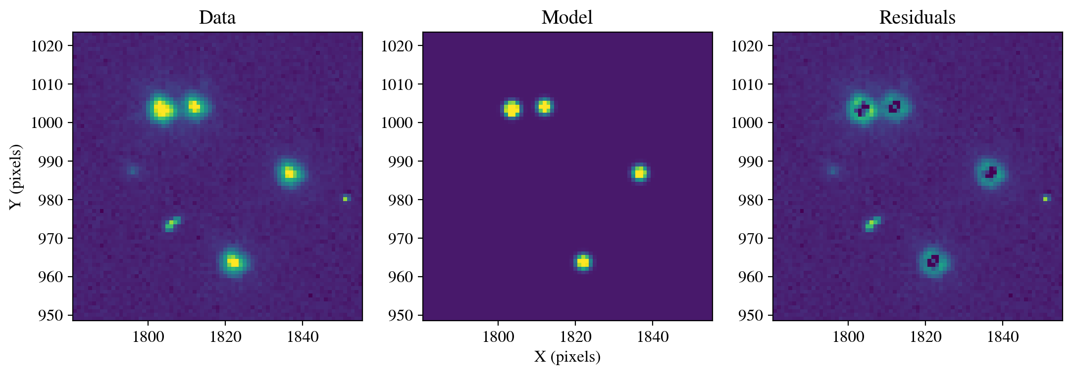
Figure saved as: /home/runner/work/hst_notebooks/hst_notebooks/notebooks/WFC3/point_spread_function/plot/fig2_gaussian_model.pdf

Aperture Photometry (after subtraction):

 id xcenter ycenter aperture_sum total_background flux_background_sub
      pix     pix                                                    
--- ------- ------- ------------ ---------------- -------------------
  1 1822.05  963.68     13226.04           989.01            12237.03
  2 1836.63  986.73     12631.20           970.57            11660.63
  3 1803.54 1003.36     25141.91          1303.54            23838.37
  4 1812.01 1004.03     14513.20          1261.96            13251.24 

In this case, the Gaussian fit leaves significant residual flux in the stellar wings, and has oversubtracted the emission in the core. The three panels above are shown with the same minimum and maximum flux values, so the residuals can be directly compared with the data and model. In the next section, we improve this using models of HST data.

2.2 Empirical PSF Models

Table of Contents

---

The example above demonstrates how a Gaussian profile can determine reasonable centroids for stellar sources, but they fail to accurately model the radial light distribution. While it is possible to use more advanced analytical forms such as Moffat profiles, the overall shape can be more accurately represented by models constructed from bright stars in the field of view. The examples below demonstrate how to use pre-generated PSF models provided by the WFC3 team, as well as how to extract and stack stars from your observations. As described below, the pre-generated models are excellent for precision astrometry and photometry of unresolved sources, while stacking stars can be more beneficial for accurately modeling the PSF wings and diffraction spikes.

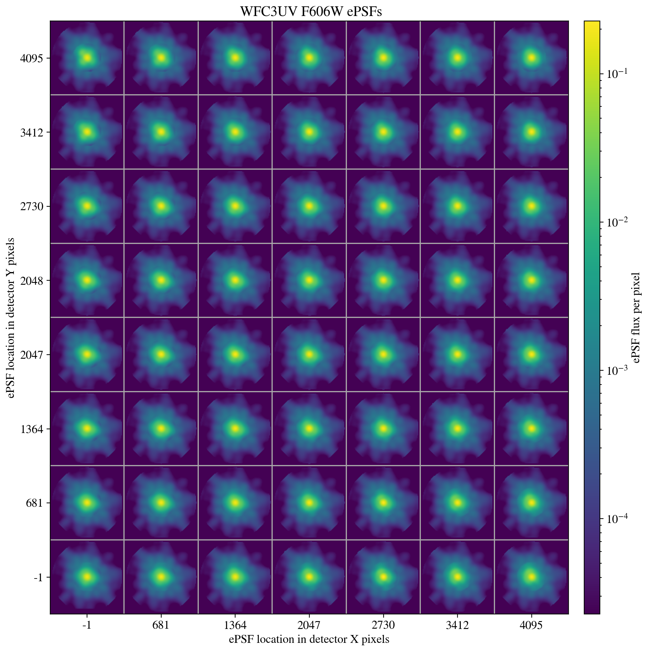
First, we display the pre-generated PSF models provided by the WFC3 team, which are stored in a standard format known as “STDPSF_WFC3”. The FITS file for each filter contains a grid of models that represents the PSF at regularly spaced intervals of a few hundred pixels across the detector, as shown below. The models are oversampled by a factor of 4x to account for the fact that the morphology of the PSF changes depending on where a star falls within a given pixel. These models are tapered to zero flux at large radii to prevent discontinuities in image subtraction, at the expense of PSF wing accuracy. The specific details of these models are provided on the WFC3 PSF webpage, as well as in WFC3 ISR 2016-12. The models are retrieved from https://www.stsci.edu/~jayander/HST1PASS/LIB/PSFs/STDPSFs/, and we save them to the main directory for access by hst1pass.

There are also “focus-diverse” models for commonly used filters with an additional dimension containing the same grids at different focus intervals. The best fit model can be determined experimentally, or by running the hst1pass code to measure the focus. However, if there are a sufficient number of stars to measure the focus then hst1pass can “perturb” the pre-generated PSF models to best match the data. As this approach is generalized for any filter we do not use the focus-diverse models in this notebook. Users can find information in WFC3 ISR 2018-14. In addition, similar focus-diverse models exist for ACS as described in ACS ISR 2023-06.

Finally, in the examples below we complete a single iteration in the PSF fitting, but it is possible to recover faint blended stars iteratively using IterativePSFPhotometry.

hst_wfc3_f606w_psf_model = download_psf_model(psfs_dir, 'WFC3UV', 'F606W')
hdul = fits.open(psfs_dir+hst_wfc3_f606w_psf_model, ignore_missing_end=True)
setup_matplotlib('notebook', 1.4)
psfgrid = STDPSFGrid(psfs_dir+hst_wfc3_f606w_psf_model).plot_grid()
save_figure(psfgrid, plot_dir+'fig3_empirical_grid.pdf', True)

Downloading: https://www.stsci.edu/~jayander/HST1PASS/LIB/PSFs/STDPSFs/WFC3UV/STDPSF_WFC3UV_F606W.fits
Validation complete, the PSF file is readable.

Figure saved as: /home/runner/work/hst_notebooks/hst_notebooks/notebooks/WFC3/point_spread_function/plot/fig3_empirical_grid.pdf

2.2.1 Default Models

Table of Contents

---

First, we can simply use the pre-generated PSF models provided by the WFC3 team. In many cases, these models will be sufficient for measuring very accurate astrometry and photometry of stellar sources in individual exposures (FLTs/FLCs) without further modifications. We utilize functions within the Astropy-affiliated photutils package to read the models into a recognized format for the PSF fitter. As noted in the packages documentation, for ACS/WFC and WFC3/UVIS the detector value should be “1” for WFC2, UVIS2 (sci, 1), and “2” for WFC1, UVIS1 (sci, 2).

In the examples below we only utilize the ['SCI', 1] extension of the science image, so the hst1pass and array image coordinates will match. When analyzing ['SCI', 2] (k = 1 in hst1pass catalogs) users must subtract 2048 from the hst1pass y coordinates so they match the array coordinates. This is because hst1pass detects over the full 4096x2048 dimensions of the detector, but each chip is read in as a 2048x2048 array.

We now read in the model and use it with the PSF fitter to calculate the best fit model and residuals.

model_uvis1 = GriddedPSFModel.read(psfs_dir+hst_wfc3_f606w_psf_model, format='stdpsf', detector_id=2)
# model_uvis2 = GriddedPSFModel.read(psfs_dir+hst_wfc3_f606w_psf_model, format='stdpsf', detector_id=1) # Would be used for UVIS2.
photometry, psfphot = calculate_photometry(sci_data, sources, psf_model=model_uvis1)
resid = psfphot.make_residual_image(sci_data, (9, 9))
figure = plot_psf_results(sci_data, resid, 1818, 986, cutout_size)
save_figure(figure, plot_dir+'fig4_empirical_default.pdf', True)
calculate_residuals(resid, sources)

PSF Photometry (before subtraction):

 id  x_fit   y_fit  flux_fit  qfit
--- ------- ------- -------- -----
  1 1822.10  963.69 25294.97 0.402
  2 1836.67  986.75 24332.85 0.398
  3 1803.57 1003.39 47571.73 0.400
  4 1812.04 1004.05 24024.78 0.418

Figure saved as: /home/runner/work/hst_notebooks/hst_notebooks/notebooks/WFC3/point_spread_function/plot/fig4_empirical_default.pdf

Aperture Photometry (after subtraction):

 id xcenter ycenter aperture_sum total_background flux_background_sub
      pix     pix                                                    
--- ------- ------- ------------ ---------------- -------------------
  1 1822.05  963.68      8494.69           989.01             7505.68
  2 1836.63  986.73      8079.31           970.57             7108.74
  3 1803.54 1003.36     15985.75          1311.52            14674.23
  4 1812.01 1004.03      9743.71          1271.65             8472.07 

2.2.2 Focus Perturbation

Table of Contents

---

In the case above, the pre-generated PSF model subtraction has substantial flux remaining in the residual image. We can use the perturbation feature within hst1pass to modify the shape of the PSF to account for the focus of these specific observations, as well as other effects such as minor modulations due to guiding accuracy. As described in Section 3.3 of WFC3 ISR 2022-05, the routine has a PERT option that can modify the library PSF if there are at least 10 relatively bright, isolated stars in the field. If PERT=1, then hst1pass constructs a single PSF that applies across the entire image. This often provides the best results, but PERT=2 can be specified to generate an NxN array of PSFs spaced evenly across the detector. This requires ample bright, isolated stars across the detector. In general, it is recommended that users begin with the unaltered PSFs before utilizing the focus or spatially-dependent perturbed PSFs. The perturbed models have a small effect on astrometry and moderate on photometry.

The commands below assume that you have followed the instructions for installing hst1pass given in the Environment Setup section. The executable can be in the same directory as assumed below, or you can provide the full path to the location of the executable. We now attempt to compile and call hst1pass with PERT=1 to construct a single perturbed PSF model that applies at all locations on the detector. We make a copy of the model because it will be overwritten by hst1pass, but call the original file for compatibility with GriddedPSFModel.

if not os.path.exists(code_dir+'hst1pass.e'):
    os.chdir(code_dir)
    !gfortran hst1pass.2023.11.07_v1f.F -o hst1pass.e
    print('The hst1pass.e has been compiled.')
else:
    print('The executable already exists.')

The hst1pass.e has been compiled.

We now call hst1pass and specify the minimum isolation distance in pixels from the next brightest pixel (HMIN), the minimum source flux in counts in the central pixel (FMIN), and the maximum source flux in the central pixel (PMAX). These arguments are followed by the OUT output columns of the resulting catalog, followed by the PSF model to use, and the FLC file to be analyzed.

os.chdir(data_dir)
!./../hst1pass.e HMIN=5 FMIN=1000.0 PMAX=66000.0 PERT=1 OUT=xympqks PSF=./../psfs/STDPSF_WFC3UV_F606W.fits id8048dyq_flc.fits
shutil.copy('id8048dyq_psf.fits', psfs_dir+'id8048dyq_psf_pert1.fits')
shutil.copy('id8048dyq_flc.xympqks', 'id8048dyq_flc_pert1.xympqks')
clear_output()

Read in the perturbed model and examine the residuals.

psf_model_perturbed_1 = data_dir+'id8048dyq_psf.fits'
model_uvis1 = GriddedPSFModel.read(psf_model_perturbed_1, format='stdpsf', detector_id=2)
# model_uvis2 = GriddedPSFModel.read(psf_model_perturbed_1, format='stdpsf', detector_id=1) # Would be used for UVIS2.
photometry, psfphot = calculate_photometry(sci_data, sources, psf_model=model_uvis1)
resid = psfphot.make_residual_image(sci_data, (9, 9))
figure = plot_psf_results(sci_data, resid, 1818, 986, cutout_size)
save_figure(figure, plot_dir+'fig5_empirical_focus.pdf', True)
calculate_residuals(resid, sources)

PSF Photometry (before subtraction):

 id  x_fit   y_fit  flux_fit  qfit
--- ------- ------- -------- -----
  1 1822.09  963.70 30906.12 0.114
  2 1836.67  986.76 29729.16 0.113
  3 1803.57 1003.39 57980.02 0.111
  4 1812.03 1004.05 29306.51 0.130

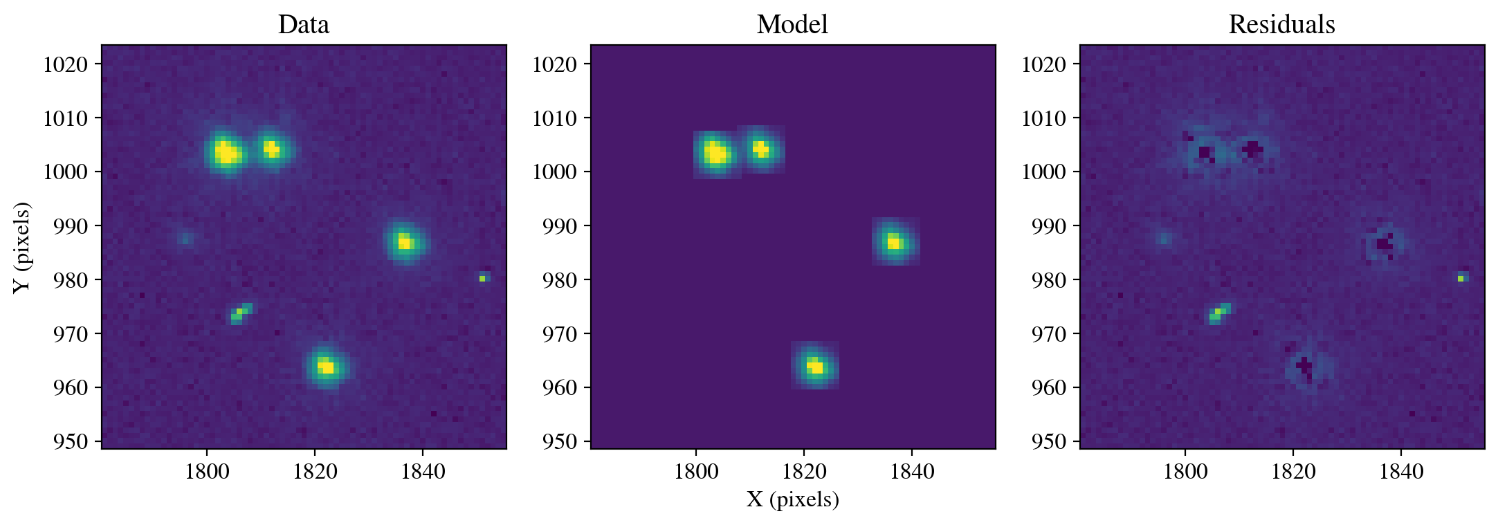
Figure saved as: /home/runner/work/hst_notebooks/hst_notebooks/notebooks/WFC3/point_spread_function/plot/fig5_empirical_focus.pdf

Aperture Photometry (after subtraction):

 id xcenter ycenter aperture_sum total_background flux_background_sub
      pix     pix                                                    
--- ------- ------- ------------ ---------------- -------------------
  1 1822.05  963.68      2915.49           989.01             1926.48
  2 1836.63  986.73      2695.88           970.57             1725.31
  3 1803.54 1003.36      5548.21          1303.54             4244.68
  4 1812.01 1004.03      3972.81          1266.56             2706.25 

We see that the residual flux is smaller than when using the default models, and visually the subtraction is improved by accounting for the focus of these observations.

2.2.3 Spatial Perturbation

Table of Contents

---

In general, using hst1pass with PERT=1 to construct a single, focus-dependent PSF model that applies across the detector will provide the best results. However, for specialized use cases with many bright, isolated stars that are located near one location on the detector, or dispersed across the entire detector, hst1pass can create a spatially-dependent PSF model in the same NxN array format as the STDPSF_WFC3 standard models. We now use hst1pass with PERT=2 to generate a grid of spatially-dependent PSF models optimized for the focus of this exposure at each location on the detector.

os.chdir(data_dir)
!./../hst1pass.e HMIN=5 FMIN=1000.0 PMAX=66000.0 PERT=2 OUT=xympqks PSF=./../psfs/STDPSF_WFC3UV_F606W.fits id8048dyq_flc.fits
shutil.copy('id8048dyq_psf.fits', psfs_dir+'id8048dyq_psf_pert2.fits')
shutil.copy('id8048dyq_flc.xympqks', 'id8048dyq_flc_pert2.xympqks')
clear_output()

Read in the perturbed model and examine the residuals.

psf_model_perturbed_2 = data_dir+'id8048dyq_psf.fits'
model_uvis1 = GriddedPSFModel.read(psf_model_perturbed_2, format='stdpsf', detector_id=2)
# model_uvis2 = GriddedPSFModel.read(psf_model_perturbed_2, format='stdpsf', detector_id=1) # Would be used for UVIS 2.
photometry, psfphot = calculate_photometry(sci_data, sources, psf_model=model_uvis1)
resid = psfphot.make_residual_image(sci_data, (9, 9))
figure = plot_psf_results(sci_data, resid, 1818, 986, cutout_size)
save_figure(figure, plot_dir+'fig6_empirical_spatial.pdf', True)
calculate_residuals(resid, sources)

PSF Photometry (before subtraction):

 id  x_fit   y_fit  flux_fit  qfit
--- ------- ------- -------- -----
  1 1822.09  963.70 30702.24 0.123
  2 1836.67  986.76 29502.78 0.122
  3 1803.57 1003.39 57540.93 0.121
  4 1812.03 1004.05 29127.32 0.139

Figure saved as: /home/runner/work/hst_notebooks/hst_notebooks/notebooks/WFC3/point_spread_function/plot/fig6_empirical_spatial.pdf

Aperture Photometry (after subtraction):

 id xcenter ycenter aperture_sum total_background flux_background_sub
      pix     pix                                                    
--- ------- ------- ------------ ---------------- -------------------
  1 1822.05  963.68      3107.83           989.01             2118.82
  2 1836.63  986.73      2914.79           970.57             1944.22
  3 1803.54 1003.36      5977.71          1303.54             4674.17
  4 1812.01 1004.03      4197.96          1276.73             2921.23 

Interestingly, the residual flux is minutely larger when using the spatially-dependent model with this dataset, which can be seen by comparing the flux_background_sub values for each star in the above tables. This is primarily due to the fact that there are an insufficient number of bright, isolated stars to accurately constrain the PSF model at each location on the detector. Thus, the best solution is produced by using PERT=1 with hst1pass.

In summary, the default models will work well for many science cases. If there are substantial residuals, then hst1pass can apply a perturbation that slightly changes the PSF model shape to compensate for different focus positions (PERT=1). It is also possible to account for both the focus and spatial variation of the PSF across the detector (PERT=2). However, changes in the PSF due to focus are generally more significant than the spatial variations unless sources are close to the edges of the detector, and accounting for both effects requires a very large number of bright, isolated stars.

Finally, we copy the hst1pass catalog generated with PERT=1 so the best catalog is used later in the stacking analysis. We also copy the catalog to the main directory so users who are unable to run hst1pass can complete the tutorial. Users can change this cell to experiment with catalogs made by running hst1pass with different settings.

This concludes the section on using empirical PSF models provided by the WFC3 team.

if os.path.exists(data_dir+'id8048dyq_flc_pert1.xympqks'):
    shutil.copy(data_dir+'id8048dyq_flc_pert1.xympqks', data_dir+'id8048dyq_flc.xympqks') # Used below for source selection.
else:
    shutil.copy(code_dir+'id8048dyq_flc.xympqks', data_dir+'id8048dyq_flc.xympqks') # Included in the Github repository.

2.3 Stacked PSF Models

Table of Contents

---

The empirical models used above that are provided by the WFC3 team can provide excellent fits at the exposure level for very accurate astrometry and photometry. However, these models have three limitations for specific science cases. First, the models are intentionally tapered to zero flux at large radii to prevent oversubtraction and fitting of noise at large radii, which means they cannot accurately capture very extended emission of bright sources. Second, while these models are available for the majority of commonly used filters on WFC3, models are not available for more specialized narrowband and quadrant filters. Third, these models are generated in the exposure frame, and so do not accurately represent the PSF in drizzled image mosaics, which will differ depending on how the drizzle was created.

With these considerations, we now explore extracting and stacking stars from both individual exposures and drizzled mosaics. Stacking a large number of sources allows for efficient outlier rejection and can produce a high quality PSF that extends to large radii, but can inherently smear or broaden the PSF at a miniscule level depending on how the sources are aligned. In this example, we will first extract stars from our image of Omega Cen and stack them to produce a PSF model. Next, we will examine the case where there are insufficient stars in an image, and retrieve stellar cutouts from the MAST database to construct a model. In this case the images have a very low background flux, but images with a high background would require users to background subtract their data and/or PSF model for proper fitting and photometric accuracy.

In summary, users may wish to stack stars if 1) there is no empirical model available for their filter, 2) they are interested in extended wing emission and diffraction spikes, or 3) they need to generate a PSF model for a drizzled mosaic, including those with diffraction spikes at multiple angles. Users can stack stars extracted from their images, or use the MAST database cutout service to retrieve observations of a similar focus and quality for their science. We will use the hst1pass catalogs produced above for examples on the exposure level, which are the same as the centroids provided by the MAST cutout service, but users can provide coordinates from an external catalog (e.g. SourceExtractor, photutils) if desired.

2.3.1 Stellar Stacks

Table of Contents

---

In this example, we use the hst1pass catalog to extract and stack stars from the FLC exposure of Omega Centauri. The hst1pass catalog columns are described in Section 2.3 of WFC3 ISR 2022-05 and include x and y detector coordinates, m:magnitude, p:peak flux, q:quality of fit, k:chip number, and s:sky value. We note that running hst1pass is not required, and users can use an external catalog generated with photutils or other packages provided the catalog contains accurate x and y coordinates. An example of this is shown in the section on Drizzle PSF Models.

We first read the hst1pass catalog and select bright stars with excellent qfit values on chip two. We also require a low sky value to remove some cutouts with many neighboring stars, and create a buffer around the edges of the detector so all cutouts contain a full array of data. The rpix parameter sets the radius of the cutout in pixels. For example, rpix = 19 produces a 39x39 pixel PSF model, corresponding to a size of 1.54\(\times\)1.54 arcseconds.

NOTE: Users who are unable to run hst1pass can continue the tutorial using the included catalog file id8048dyq_flc.xympqks that is automatically copied to the data_dir.

# Read the hst1pass catalog and select stars.
hst1pass_cat = Table.read(data_dir+'id8048dyq_flc.xympqks', 
                          format='ascii', 
                          guess=False, 
                          fast_reader=False, 
                          data_start=1, 
                          names=['x', 'y', 'm', 'p', 'q', 'k', 's'])

print('The original catalog has', len(hst1pass_cat), 'entries.')

rpix = 19 # Set the radius in pixels for the cutouts and resulting PSF.

# Select sources with specific brightness, qfit, and location criteria.
mask = (
    (hst1pass_cat['x'] > rpix) &
    (hst1pass_cat['x'] < 4096.0-rpix) &
    (hst1pass_cat['y'] > rpix) &
    (hst1pass_cat['y'] < 2048.0-rpix) &
    (hst1pass_cat['p'] >= 10000.0) &
    (hst1pass_cat['p'] <= 63300.0) &
    (hst1pass_cat['q'] <= 0.035) &
    (hst1pass_cat['k'] == 2) &
    (hst1pass_cat['s'] <= 100.0)
)

hst1pass_cat = hst1pass_cat[mask]

star_ids = list(range(len(hst1pass_cat)))

hst1pass_cat

The original catalog has 2397 entries.

Table length=34

x	y	m	p	q	k	s
float64	float64	float64	float64	float64	int64	float64
1286.7318	32.5184	-13.268	21134.07	0.025	2	16.4
929.775	33.3364	-12.665	14191.36	0.023	2	16.39
1241.7439	60.5701	-14.294	55280.03	0.024	2	29.08
911.0856	64.5218	-13.009	18216.32	0.027	2	13.52
731.933	73.6137	-12.53	12454.2	0.033	2	15.09
1187.3088	135.9943	-13.123	21676.56	0.031	2	15.37
444.3915	242.3671	-14.106	46620.75	0.03	2	29.63
755.6099	291.1403	-13.051	20003.39	0.025	2	15.43
305.463	393.9442	-13.474	29141.48	0.028	2	15.78
816.5427	430.8998	-13.917	40621.04	0.032	2	19.44
...	...	...	...	...	...	...
790.3328	1556.8351	-12.878	17708.8	0.03	2	14.56
527.3823	1618.9103	-12.904	18090.87	0.027	2	16.95
474.7753	1697.0492	-12.765	16793.74	0.035	2	14.77
931.1865	1793.3379	-12.479	11992.43	0.032	2	15.93
958.9084	1837.1936	-13.257	26489.8	0.034	2	16.6
1210.0345	1857.8748	-12.383	12469.67	0.03	2	15.13
660.1707	1879.8505	-12.358	11823.76	0.034	2	10.48
976.6851	1930.8593	-13.243	24624.58	0.032	2	19.3
315.5191	2009.2579	-12.381	10412.01	0.025	2	16.62
1206.7129	2013.9739	-12.821	17920.06	0.031	2	16.08

The make_cutouts function uses the science image and catalog coordinates to extract cutouts of the stars meeting the criteria set by the mask in the cell above. The scale_stars option will normalize the flux of each star, which is generally recommended for proper averaging. The sub_pixel option uses the user-supplied x and y coordinates to align the cutouts at the subpixel level and should always be used except for testing. When verbose is True, additional diagnostic messages will be printed. Specifically, after performing the subpixel alignment, the function will calculate the center of mass using the inner five pixels. This value should generally be very close to the user-suppled rpix value, but will deviate minutely depending on how the x and y centroids were calculated.

star_cutouts = make_cutouts(image=sci_data, 
                            star_ids=star_ids, 
                            xis=hst1pass_cat['x'], 
                            yis=hst1pass_cat['y'], 
                            rpix=rpix, 
                            scale_stars=True, 
                            sub_pixel=True, 
                            show_figs=True, 
                            verbose=True)

Calling make_cutouts with 34 sources.

Star ID 0: (x,y) = (1287, 33)
The read in x, y are: 1286.7318 32.5184
x_shift, y_shift = 0.2682 0.4816
Before shift centroid = 18.8847 18.7924
After shift centroid =  19.0063 18.9988
The subimage peak flux (x,y) = (19), 19)
Scaling the stars peak flux to unity...

Star ID 1: (x,y) = (930, 33)
The read in x, y are: 929.775 33.3364
x_shift, y_shift = 0.225 -0.3364
Before shift centroid = 18.9357 19.1347
After shift centroid =  19.0061 19.0025
The subimage peak flux (x,y) = (19), 19)
Scaling the stars peak flux to unity...

Star ID 2: (x,y) = (1242, 61)
The read in x, y are: 1241.7439 60.5701
x_shift, y_shift = 0.2561 0.4299
Before shift centroid = 18.886 18.8118
After shift centroid =  19.0044 18.9991
The subimage peak flux (x,y) = (19), 19)
Scaling the stars peak flux to unity...

Star ID 3: (x,y) = (911, 65)
The read in x, y are: 911.0856 64.5218
x_shift, y_shift = -0.0856 0.4782
Before shift centroid = 19.0035 18.8021
After shift centroid =  19.0049 19.007
The subimage peak flux (x,y) = (19), 19)
Scaling the stars peak flux to unity...

Star ID 4: (x,y) = (732, 74)
The read in x, y are: 731.933 73.6137
x_shift, y_shift = 0.067 0.3863
Before shift centroid = 18.9476 18.8263
After shift centroid =  18.999 18.9989
The subimage peak flux (x,y) = (19), 19)
Scaling the stars peak flux to unity...

Star ID 5: (x,y) = (1187, 136)
The read in x, y are: 1187.3088 135.9943
x_shift, y_shift = -0.3088 0.0057
Before shift centroid = 19.1374 19.0164
After shift centroid =  19.0099 19.0035
The subimage peak flux (x,y) = (19), 19)
Scaling the stars peak flux to unity...

Star ID 6: (x,y) = (444, 242)
The read in x, y are: 444.3915 242.3671
x_shift, y_shift = -0.3915 -0.3671
Before shift centroid = 19.1774 19.1698
After shift centroid =  19.0065 19.0035
The subimage peak flux (x,y) = (19), 19)
Scaling the stars peak flux to unity...

Star ID 7: (x,y) = (756, 291)
The read in x, y are: 755.6099 291.1403
x_shift, y_shift = 0.3901 -0.1403
Before shift centroid = 18.8458 19.0364
After shift centroid =  19.0029 19.0021
The subimage peak flux (x,y) = (19), 19)
Scaling the stars peak flux to unity...

Star ID 8: (x,y) = (305, 394)
The read in x, y are: 305.463 393.9442
x_shift, y_shift = -0.463 0.0558
Before shift centroid = 19.1986 19.0098
After shift centroid =  19.0025 19.0017
The subimage peak flux (x,y) = (19), 19)
Scaling the stars peak flux to unity...

Star ID 9: (x,y) = (817, 431)
The read in x, y are: 816.5427 430.8998
x_shift, y_shift = 0.4573 0.1002
Before shift centroid = 18.8081 18.9378
After shift centroid =  18.9966 18.9982
The subimage peak flux (x,y) = (19), 19)
Scaling the stars peak flux to unity...

Star ID 10: (x,y) = (479, 436)
The read in x, y are: 478.8024 436.3226
x_shift, y_shift = 0.1976 -0.3226
Before shift centroid = 18.9452 19.1247
After shift centroid =  19.0035 18.9966
The subimage peak flux (x,y) = (19), 19)
Scaling the stars peak flux to unity...

Star ID 11: (x,y) = (856, 598)
The read in x, y are: 856.0377 598.0248
x_shift, y_shift = -0.0377 -0.0248
Before shift centroid = 19.0163 19.009
After shift centroid =  18.9999 18.997
The subimage peak flux (x,y) = (19), 19)
Scaling the stars peak flux to unity...

Star ID 12: (x,y) = (521, 649)
The read in x, y are: 521.2008 649.2875
x_shift, y_shift = -0.2008 -0.2875
Before shift centroid = 19.1048 19.1326
After shift centroid =  19.0113 19.0037
The subimage peak flux (x,y) = (19), 19)
Scaling the stars peak flux to unity...

Star ID 13: (x,y) = (303, 788)
The read in x, y are: 303.2865 788.0764
x_shift, y_shift = -0.2865 -0.0764
Before shift centroid = 19.1306 19.0447
After shift centroid =  19.0061 18.9992
The subimage peak flux (x,y) = (19), 19)
Scaling the stars peak flux to unity...

Star ID 14: (x,y) = (913, 851)
The read in x, y are: 913.4318 850.7266
x_shift, y_shift = -0.4318 0.2734
Before shift centroid = 19.1593 18.9233
After shift centroid =  19.0025 18.9992
The subimage peak flux (x,y) = (19), 19)
Scaling the stars peak flux to unity...

Star ID 15: (x,y) = (563, 937)
The read in x, y are: 562.5058 936.9977
x_shift, y_shift = 0.4942 0.0023
Before shift centroid = 18.795 18.9684
After shift centroid =  19.0012 18.9994
The subimage peak flux (x,y) = (19), 19)
Scaling the stars peak flux to unity...

Star ID 16: (x,y) = (749, 939)
The read in x, y are: 748.6302 939.3118
x_shift, y_shift = 0.3698 -0.3118
Before shift centroid = 18.8702 19.1027
After shift centroid =  19.0037 18.9953
The subimage peak flux (x,y) = (19), 19)
Scaling the stars peak flux to unity...

Star ID 17: (x,y) = (359, 1052)
The read in x, y are: 359.2828 1051.7438
x_shift, y_shift = -0.2828 0.2562
Before shift centroid = 19.1002 18.9059
After shift centroid =  19.0007 18.9978
The subimage peak flux (x,y) = (19), 19)
Scaling the stars peak flux to unity...

Star ID 18: (x,y) = (426, 1065)
The read in x, y are: 425.7358 1065.4231
x_shift, y_shift = 0.2642 -0.4231
Before shift centroid = 18.9258 19.1639
After shift centroid =  19.0028 18.9911
The subimage peak flux (x,y) = (19), 19)
Scaling the stars peak flux to unity...

Star ID 19: (x,y) = (263, 1150)
The read in x, y are: 262.7981 1150.071
x_shift, y_shift = 0.2019 -0.071
Before shift centroid = 18.9177 19.0177
After shift centroid =  19.0011 18.9959
The subimage peak flux (x,y) = (19), 19)
Scaling the stars peak flux to unity...

Star ID 20: (x,y) = (551, 1302)
The read in x, y are: 551.4668 1301.9565
x_shift, y_shift = -0.4668 0.0435
Before shift centroid = 19.2049 19.0135
After shift centroid =  19.0076 18.9979
The subimage peak flux (x,y) = (19), 19)
Scaling the stars peak flux to unity...

Star ID 21: (x,y) = (229, 1383)
The read in x, y are: 229.1015 1383.1074
x_shift, y_shift = -0.1015 -0.1074
Before shift centroid = 19.0533 19.0514
After shift centroid =  19.0053 18.999
The subimage peak flux (x,y) = (19), 19)
Scaling the stars peak flux to unity...

Star ID 22: (x,y) = (179, 1423)
The read in x, y are: 179.4781 1422.6169
x_shift, y_shift = -0.4781 0.3831
Before shift centroid = 19.1675 18.8799
After shift centroid =  19.0026 18.9977
The subimage peak flux (x,y) = (19), 19)
Scaling the stars peak flux to unity...

Star ID 23: (x,y) = (566, 1489)
The read in x, y are: 566.2279 1489.3282
x_shift, y_shift = -0.2279 -0.3282
Before shift centroid = 19.1235 19.1527
After shift centroid =  19.0141 19.0014
The subimage peak flux (x,y) = (19), 19)
Scaling the stars peak flux to unity...

Star ID 24: (x,y) = (790, 1557)
The read in x, y are: 790.3328 1556.8351
x_shift, y_shift = -0.3328 0.1649
Before shift centroid = 19.1344 18.9511
After shift centroid =  19.0037 18.9955
The subimage peak flux (x,y) = (19), 19)
Scaling the stars peak flux to unity...

Star ID 25: (x,y) = (527, 1619)
The read in x, y are: 527.3823 1618.9103
x_shift, y_shift = -0.3823 0.0897
Before shift centroid = 19.168 18.9865
After shift centroid =  19.0049 18.9978
The subimage peak flux (x,y) = (19), 19)
Scaling the stars peak flux to unity...

Star ID 26: (x,y) = (475, 1697)
The read in x, y are: 474.7753 1697.0492
x_shift, y_shift = 0.2247 -0.0492
Before shift centroid = 18.9109 19.0056
After shift centroid =  19.0019 18.9965
The subimage peak flux (x,y) = (19), 19)
Scaling the stars peak flux to unity...

Star ID 27: (x,y) = (931, 1793)
The read in x, y are: 931.1865 1793.3379
x_shift, y_shift = -0.1865 -0.3379
Before shift centroid = 19.1101 19.1602
After shift centroid =  19.0138 19.0017
The subimage peak flux (x,y) = (19), 19)
Scaling the stars peak flux to unity...

Star ID 28: (x,y) = (959, 1837)
The read in x, y are: 958.9084 1837.1936
x_shift, y_shift = 0.0916 -0.1936
Before shift centroid = 18.9805 19.0775
After shift centroid =  19.0052 18.9992
The subimage peak flux (x,y) = (19), 19)
Scaling the stars peak flux to unity...

Star ID 29: (x,y) = (1210, 1858)
The read in x, y are: 1210.0345 1857.8748
x_shift, y_shift = -0.0345 0.1252
Before shift centroid = 19.0045 18.9432
After shift centroid =  18.9983 18.9968
The subimage peak flux (x,y) = (19), 19)
Scaling the stars peak flux to unity...

Star ID 30: (x,y) = (660, 1880)
The read in x, y are: 660.1707 1879.8505
x_shift, y_shift = -0.1707 0.1495
Before shift centroid = 19.0638 18.9441
After shift centroid =  19.001 18.999
The subimage peak flux (x,y) = (19), 19)
Scaling the stars peak flux to unity...

Star ID 31: (x,y) = (977, 1931)
The read in x, y are: 976.6851 1930.8593
x_shift, y_shift = 0.3149 0.1407
Before shift centroid = 18.8558 18.907
After shift centroid =  18.9977 18.9887
The subimage peak flux (x,y) = (19), 19)
Scaling the stars peak flux to unity...

Star ID 32: (x,y) = (316, 2009)
The read in x, y are: 315.5191 2009.2579
x_shift, y_shift = 0.4809 -0.2579
Before shift centroid = 18.8206 19.0709
After shift centroid =  19.0095 18.9974
The subimage peak flux (x,y) = (19), 19)
Scaling the stars peak flux to unity...

Star ID 33: (x,y) = (1207, 2014)
The read in x, y are: 1206.7129 2013.9739
x_shift, y_shift = 0.2871 0.0261
Before shift centroid = 18.8711 18.9623
After shift centroid =  19.0009 18.9924
The subimage peak flux (x,y) = (19), 19)
Scaling the stars peak flux to unity...

The stack_cutouts function then combines the array of cutouts into a single mean or median stack, with the option to normalize the flux. In general, using a stack_type of median is recommended to reject contaminating sources. Similarly, setting scale_flux to True is recommended so that all sources have normalized fluxes, which prevents biased weighting by S/N and produces a normalized PSF, which is typically required by many photometric tools.

star_stack = stack_cutouts(star_cutouts, 
                           rpix=rpix, 
                           stack_type='median', 
                           scale_flux=True, 
                           export_file=psfs_dir+'hst_wfc3_uvis_f606w_star_psf_model.fits')

Calling stack_cutouts with 34 sources.

Creating a median image stack.
Scaling the total flux to one.
The total image flux is = 1.0

Finally, we provide our stacked model to the photutils FittableImageModel function, which allows it to be used with the PSF fitter. While the core emission was better fit using the empirical models in the previous section, using the stacked model that is not tapered to zero flux allows us to fit out to large radii, which is set to 19 pixels below.

star_stack_psf = FittableImageModel(star_stack[0])
photometry, psfphot = calculate_photometry(sci_data, sources, psf_model=star_stack_psf)
resid = psfphot.make_residual_image(sci_data, (19, 19))
figure = plot_psf_results(sci_data, resid, 1818, 986, cutout_size)
save_figure(figure, plot_dir+'fig7_star_stack.pdf', True)
calculate_residuals(resid, sources)

PSF Photometry (before subtraction):

 id  x_fit   y_fit  flux_fit  qfit
--- ------- ------- -------- -----
  1 1822.07  963.70 38502.79 0.089
  2 1836.67  986.76 37021.88 0.089
  3 1803.57 1003.38 72023.97 0.083
  4 1812.01 1004.04 36210.23 0.094

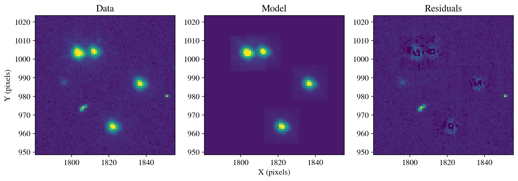
Figure saved as: /home/runner/work/hst_notebooks/hst_notebooks/notebooks/WFC3/point_spread_function/plot/fig7_star_stack.pdf

Aperture Photometry (after subtraction):

 id xcenter ycenter aperture_sum total_background flux_background_sub
      pix     pix                                                    
--- ------- ------- ------------ ---------------- -------------------
  1 1822.05  963.68      1629.97           726.81              903.16
  2 1836.63  986.73      1477.78           725.84              751.94
  3 1803.54 1003.36      2666.58           750.59             1915.99
  4 1812.01 1004.03      1520.94           769.32              751.61 

2.3.2 MAST Stacks

Table of Contents

---

The example above demonstrates how to extract and stack stars from a provided exposure. However, in many cases there may be an insufficient number of stars to create a high-quality median stack. In those cases, users can utilize the MAST cutout database described in WFC3 ISR 2021-12, with access instructions provided on the PSF Search webpage. The MAST API commands are listed on this webpage, with parameter options on this webpage. The examples below utilize sections of code from the download_psf_cutouts.ipynb developed by Dauphin et al. (in preparation). In this case, we set limits on the x and y detector locations, quality of fit, exposure time, isolation index, integrated flux (in electrons for WFC3/UVIS and WFPC2, and in electrons per second for WFC3/IR), the central pixel flux, sky flux, and exclude subarrays. The stellar centroids provided in the MAST database were calculated using hst1pass and the empirical PSF models described in Section 2.2. See WFC3 ISR 2021-12 for additional information.

NOTE: We explicitly assume that users have familiarized themselves with the contents of the "download_psf_cutouts.ipynb" notebook for this section.

os.chdir(code_dir)

# Searching a larger radius around the cutout for a sufficient number of stars.
x_min_max = mast_api_psf.set_min_max(1818-cutout_size*5, 1818+cutout_size*5)
y_min_max = mast_api_psf.set_min_max(986-cutout_size*5, 986+cutout_size*5)
qfit_min_max = mast_api_psf.set_min_max(0.0, 0.05)
exp_time = mast_api_psf.set_min_max(10, 30000)
iso_index = mast_api_psf.set_min_max(20, 4096)
psf_flux = mast_api_psf.set_min_max(2000, 1000000000) # This is an integrated value so set an arbitarily large upper bound.
pixc = mast_api_psf.set_min_max(59000, 63300)
sky_flux = mast_api_psf.set_min_max(0, 50)
focus = mast_api_psf.set_min_max(-10, 10) # Change these values to see the effects of focus.
subarray = mast_api_psf.set_min_max(0, 0)

detector = 'UVIS'

# Set the parameters, noting that the last four are not set above.
parameters = {
    'psf_x_center': x_min_max, 
    'psf_y_center': y_min_max, 
    'qfit': qfit_min_max, 
    'exptime': exp_time, 
    'iso_index': iso_index, 
    'psf_flux': psf_flux, 
    'pixc': pixc, 
    'sky': sky_flux, 
    'focus': focus, 
    'subarray': ['0'],
    'n_sat_pixels': ['0'], 
    'filter': ['F606W'], 
    'mtflag': ['0'],
}

filts = mast_api_psf.set_filters(parameters)
columns = ['id', 'rootname', 'filter', 'chip', 'exptime', 'psf_x_center', 'psf_y_center', 'pixc', 'sky', 'qfit', 'iso_index', 'subarray']
obs = mast_api_psf.mast_query_psf_database(detector=detector, filts=filts, columns=columns)
obs

Table masked=True length=50

id	rootname	filter	chip	exptime	psf_x_center	psf_y_center	pixc	sky	qfit	iso_index	subarray
int64	str9	str5	str1	float64	float64	float64	float64	float64	float64	int64	int64
26447668	icmw09v8q	F606W	2	348.0	1818.1829	1011.259	60800.44	35.04	0.034	24	0
22694839	icc303kjq	F606W	2	570.0	1958.4135	930.4946	62666.45	48.78	0.029	24	0
26385576	ibc602v7q	F606W	2	360.0	2116.5151	1143.5637	63022.99	32.91	0.05	24	0
20264574	ibc602v6q	F606W	2	360.0	2119.3423	1205.4642	60694.15	35.5	0.049	24	0
28058025	id1x15wcq	F606W	2	40.0	1881.6022	1333.9424	61112.78	49.87	0.05	24	0
23186113	ibc302j7q	F606W	2	40.0	2157.4431	1311.0704	60846.07	44.64	0.037	24	0
21965947	icc303kcq	F606W	2	560.0	1958.563	930.7289	63243.29	45.94	0.042	24	0
24883910	icqx02bvq	F606W	2	40.0	2026.3932	772.9385	62638.16	47.94	0.043	24	0
22304694	ic4j06zlq	F606W	2	40.0	1764.0898	735.2534	59308.56	43.74	0.042	24	0
22806078	ibm516fjq	F606W	2	40.0	1791.9078	762.9925	60518.07	44.16	0.044	24	0
...	...	...	...	...	...	...	...	...	...	...	...
25172815	ib2o02tbq	F606W	2	616.0	1621.2174	1220.9774	59238.68	49.37	0.043	24	0
26113796	ibnh13h2q	F606W	2	348.0	1727.7864	708.8348	61216.02	34.74	0.042	24	0
19530451	ib6v01drq	F606W	2	50.0	2077.6558	757.127	59483.89	16.67	0.045	24	0
23179989	ibc302j7q	F606W	2	40.0	1533.0767	983.4271	60506.57	45.06	0.028	24	0
22422174	ibnh11bkq	F606W	2	348.0	1716.386	869.8177	59014.58	29.06	0.039	24	0
22056475	ic8x01mfq	F606W	2	50.0	2191.8518	1087.7273	59502.78	31.68	0.035	24	0
25899457	ibcd40kvq	F606W	2	450.0	2117.457	727.3718	59853.12	42.24	0.047	24	0
26765366	ic3f22meq	F606W	2	50.0	1832.6663	1161.4025	61014.33	32.28	0.045	24	0
20277208	ib2o01ssq	F606W	2	600.0	1942.1887	944.2888	59100.43	45.41	0.048	24	0
20504234	iedx05r0q	F606W	2	415.0	2122.1753	1326.8822	62098.94	33.2	0.035	24	0

As described and detailed in the download_psf_cutouts.ipynb, the below cell constructs the filepaths for the cutouts, requests to download them from the MAST cutout service, and then extracts the files from a compressed tar folder. Finally, the filepaths for each cutout are saved to a list in path_data and passed to an array.

os.chdir(data_dir)
file_suffix = ['flc']
dataURIs = mast_api_psf.make_dataURIs(obs, detector=detector, file_suffix=file_suffix)
filename = mast_api_psf.download_request(dataURIs, filename='mastDownload.tar.gz', download_type='bundle.tar.gz')
tar = tarfile.open(filename, 'r:gz')
path_mast = tar.getnames()[0]
tar.extractall()
tar.close()
path_data = sorted(glob.glob(f'{path_mast}/*/*'))
mast_cutouts = np.array([fits.getdata(path) for path in path_data])

Found 0 subarray sources in queried data.

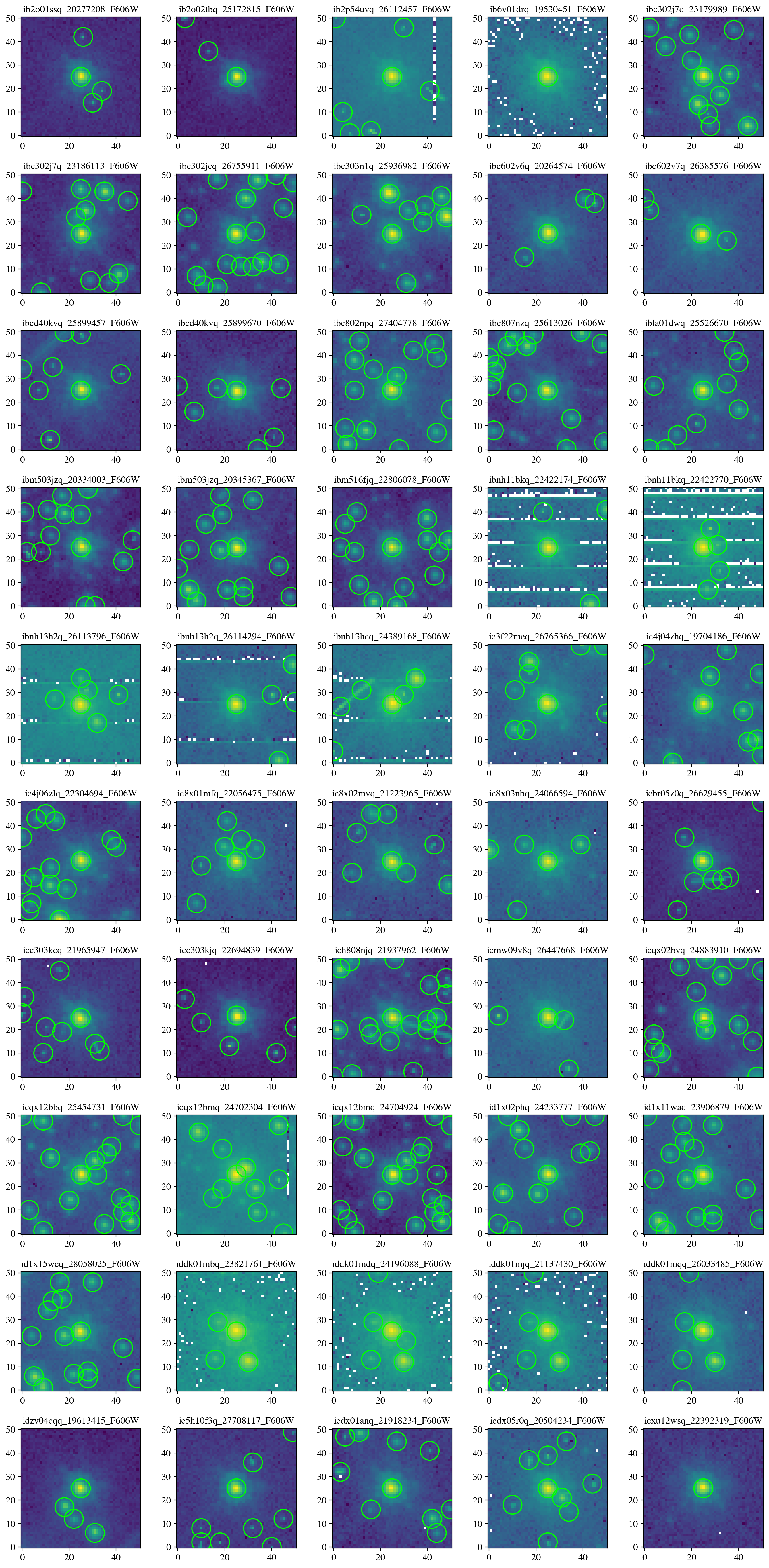
Next we visually inspect all of the downloaded cutouts, where each panel shows the cutout, and any additional sources identified at > 10\(\sigma\) above the background in green circles. Users may wish to manually or automatically filter the results to create a sample with fewer contaminants.

os.chdir(data_dir)
plot_cutout_grid(cutouts=mast_cutouts, path_data=path_data, max_cutouts=50, verbose=False)
save_figure(figure, plot_dir+'fig8_mast_grid.pdf', True)

Figure saved as: /home/runner/work/hst_notebooks/hst_notebooks/notebooks/WFC3/point_spread_function/plot/fig8_mast_grid.pdf

mast_stack = stack_cutouts(mast_cutouts, 
                           rpix=25, 
                           stack_type='median', 
                           scale_flux=True, 
                           export_file=psfs_dir+'hst_wfc3_uvis_f606w_mast_psf_model.fits')

Calling stack_cutouts with 50 sources.

Creating a median image stack.
Scaling the total flux to one.
The total image flux is = 1.0

We now use this model to perform PSF fitting and subtraction on the science image. We see that the cutouts retrieved and stacked from MAST only marginally fit the shapes of the stars in this particular exposure, similar to the results that we obtained with the empirical model before perturbation. The model could be revised by querying the MAST cutout service with different parameters and/or carefully selecting cutouts based on their FWHM. The optimal workflow will depend on the data and science goals.

mast_stack_psf = FittableImageModel(mast_stack[0])
photometry, psfphot = calculate_photometry(sci_data, sources, psf_model=mast_stack_psf)
resid = psfphot.make_residual_image(sci_data, (9, 9))
figure = plot_psf_results(sci_data, resid, 1818, 986, cutout_size)
save_figure(figure, plot_dir+'fig9_mast_stack.pdf', True)
calculate_residuals(resid, sources)

PSF Photometry (before subtraction):

 id  x_fit   y_fit  flux_fit  qfit
--- ------- ------- -------- -----
  1 1822.19  963.62 34784.45 0.260
  2 1836.74  986.68 33353.79 0.261
  3 1803.63 1003.33 64962.87 0.262
  4 1812.14 1003.96 32573.56 0.276

Figure saved as: /home/runner/work/hst_notebooks/hst_notebooks/notebooks/WFC3/point_spread_function/plot/fig9_mast_stack.pdf

Aperture Photometry (after subtraction):

 id xcenter ycenter aperture_sum total_background flux_background_sub
      pix     pix                                                    
--- ------- ------- ------------ ---------------- -------------------
  1 1822.05  963.68      7459.95           989.01             6470.94
  2 1836.63  986.73      7154.72           970.57             6184.16
  3 1803.54 1003.36     14306.16          1322.93            12983.23
  4 1812.01 1004.03      8926.97          1261.96             7665.01 

3. Drizzle PSF Models

Table of Contents

---

The examples in Section 2 apply to PSF modeling at the exposure level. However, in many cases with faint astronomical sources, multiple exposures are combined through drizzling to yield an image mosaic with increased signal-to-noise that is free from artifacts such as cosmic rays and hot pixels. This process changes the shape of the PSF due to resampling, so dedicated models are required. The process of drizzling is beyond the scope of this notebook, and users can find more information on the DrizzlePac Website, including a series of tutorial notebooks available on Github with useful examples, and a brief explanation here. In this case, it is sufficient to note that drizzling allows us to account for undersampling of the WFC3 detectors to recover the full spatial resolution of HST, and account for distortion across the field of view to provide a flux-conserved, geometrically rectified mosaic generated from the individual exposures. In this case, we combine three F606W exposures covering the same area of Omega Cen, and focused on the same four stars shown in Section 1.4.

3.1 Create Drizzle

Table of Contents

---

In the cell below, we first download the three F606W exposures and copy them to a new directory because their headers will be modified in the alignment and drizzling process. Next, we use TweakReg to find sources in common between the images and align them to the first exposure. See the TweakReg readthedocs for more information on each parameter. Note also that users can utilize hst1pass catalogs of their FLC files to perform high-accuracy alignments if there are a sufficient number of stars.

os.chdir(data_dir)

tweak_files = ['id8048e0q_flc.fits', 'id8048dyq_flc.fits', 'id8048e3q_flc.fits']

for tweak_file in tweak_files:
    print('Copying', tweak_file)
    Observations.download_file('mast:HST/product/'+tweak_file, local_path=data_dir+tweak_file, cache=True)
    shutil.copy2(tweak_file, tweak_dir)
    
os.chdir(tweak_dir)

# Call TweakReg.
tweakreg.TweakReg(tweak_files,
                  refimage=tweak_files[0],
                  expand_refcat=True,
                  clean=True,
                  interactive=False,
                  updatehdr=True,
                  reusename=False,
                  wcsname='TWEAK', 
                  descrip='HST WFC3 PSF Notebook Example',
                  catalog=tweak_files[0],
                  shiftfile=True,
                  outshifts='tweakreg_shifts.dat',
                  minobj=100,
                  searchrad=0.25,
                  searchunits='arcseconds',
                  fitgeometry='rscale',
                  nclip=5,
                  sigma=3.0,
                  imagefindcfg={'threshold': 50, 'peakmax': 62000, 'use_sharp_round': True},
                  refimagefindcfg={'threshold': 50, 'peakmax': 62000, 'use_sharp_round': True})

clear_output()

Now, we examine the TweakReg residuals to confirm they are small. The columns are filename, shift in x, shift in y, rotation in degrees, plate scale, and the x and y RMS errors on the shift. In general, RMS values below \(\approx\) 0.1 pixels are desired for a quality alignment solution. A value of NaN indicates a failure and the search parameters must be adjusted.

os.chdir(tweak_dir)
shift_table = Table.read('tweakreg_shifts.dat', 
                         format='ascii.no_header',
                         names=['file', 'dx', 'dy', 'rot', 'scale', 'xrms', 'yrms'])

formats = ['.2f', '.2f', '.3f', '.5f', '.2f', '.2f']
for i, col in enumerate(shift_table.colnames[1:]):
    shift_table[col].format = formats[i]
print(shift_table)

       file         dx    dy    rot    scale  xrms yrms
------------------ ---- ----- ------- ------- ---- ----
id8048e0q_flc.fits 0.00  0.00   0.000 1.00000 0.00 0.00
id8048dyq_flc.fits 0.10  0.06 359.999 1.00001 0.04 0.05
id8048e3q_flc.fits 0.06 -0.02   0.000 1.00001 0.04 0.04

In this case, the exposures are already well aligned as the shifts are less than \(\approx\) 0.1 pixels. Because the errors on the shifts are generally smaller than the measured shifts, we adopt the shifted values. Next, we use AstroDrizzle to combine the aligned exposures into a single mosaic. See the AstroDrizzle readthedocs for more information on each parameter.

os.chdir(tweak_dir)

for driz_file in tweak_files:
    print('Copying', driz_file, 'to the drizzle directory.')
    shutil.copy2(driz_file, driz_dir)
    
os.chdir(driz_dir)

# Run AstroDrizzle.
astrodrizzle.AstroDrizzle(tweak_files,
                          output='omega_cen_f606w_drz.fits', # The output filename.
                          wcskey='TWEAK',              # Use tweakreg WCS solution.
                          build=True,                  # Save combined SCI and WHT.
                          updatewcs=False,             # Don't run updatewcs again.
                          stepsize=1,                  # Don't interpolate the WCS.
                          num_cores=1,                 # Single core saves memory.
                          preserve=False,              # We save the files separately.
                          clean=True,                  # We don't need the mask files.
                          skysub=True,                 # Definitely subtract the sky.
                          skymethod='globalmin+match', # Recommended for diffuse data.
                          combine_type='iminmed',      # 'iminmed' for < 10 images.
                          driz_cr_corr=False,          # Save the cosmic-ray masks.
                          driz_combine=True,           # Use all images in drizzle.
                          final_wht_type='EXP',        # EXP weight for bright objects.
                          final_pixfrac=0.8,           # Fraction to shrink drops by.
                          final_units='cps')           # Set units to counts per second.

clear_output()

Finally, we can display the drizzled image and highlight the same boxed region shown in Sections 1-2. The mosaic displays a significantly smoother background than the individual exposures, without significant cosmic rays or hot pixels. Stars that were saturated in the original FLCs contain artifacts and therefore should not be stacked.

with fits.open(driz_dir+'omega_cen_f606w_drz.fits') as hdul:
    sci_driz = np.nan_to_num(hdul['SCI'].data)
print('The image dimensions are:', np.shape(sci_driz))

my_figure_size, my_fontsize = setup_matplotlib('notebook', 1.2)
figure, axes = plt.subplots(1, 1, figsize=my_figure_size)
cutout_size = 75 # 75 WFC3 UVIS pixels = 3 arcseconds.

# The same box is at: 1823.5781, 1096.5125 in the drizzled mosaic.
axes.add_patch(Rectangle((1823.5781-cutout_size/2, 1096.5125-cutout_size/2), width=cutout_size, height=cutout_size, fill=None, color='w'))
norm = simple_norm(sci_driz, 'sqrt', percent=99.8-0.2)
axes.imshow(sci_driz, cmap='gray', origin='lower', aspect='equal', interpolation='nearest', norm=norm)
plt.show()

The image dimensions are: (4520, 4345)

3.2 Stack Stars

Table of Contents

---

Next, we want to detect stars that surround the location of interest, and stack them to construct a PSF model. In this case we have a sufficient number of stars (> 10) that are near the location on the detector for which we want to construct a PSF model. In this case we select a 525\(\times\)525 pixel region near the four stars shown above. The functionality of the code below is described in more detail in Section 1.4, and the resulting stellar flux measurements can be shown by adding print(phot_table). In this case the drizzles have been background-subtracted, but images with a high background would require users to background subtract their data and/or PSF model for proper fitting and photometric accuracy.

# Calculate statistics for the background, initialize the star finder, locate the stars, and assign flux apertures.
mean, median, std = sigma_clipped_stats(sci_driz, sigma=3.0)
daofind = DAOStarFinder(threshold=2.5, fwhm=3.0, roundhi=0.5)
mask = create_mask(sci_driz, cutout_size=cutout_size*7.0, xcenter=1823, ycenter=1096)
sources = daofind(sci_driz - median, mask=mask)
positions = np.transpose((sources['xcentroid'], sources['ycentroid']))
apertures_stellar = CircularAperture(positions, r=5.0)
apertures_annulus = CircularAnnulus(positions, r_in=9, r_out=12)
phot_table = aperture_photometry(sci_driz, apertures_stellar)

# Calculate the sigma-clipped background levels and subtract that from the flux measured within the stellar aperture.
aperture_stats = ApertureStats(sci_driz, apertures_stellar, sigma_clip=None)
background_stats = ApertureStats(sci_driz, apertures_annulus, sigma_clip=SigmaClip(sigma=3.0, maxiters=10))
total_background = background_stats.median * aperture_stats.sum_aper_area.value # area of annulus.
flux_background_sub = aperture_stats.sum - total_background
phot_table['total_background'] = total_background
phot_table['flux_background_sub'] = flux_background_sub

# Display the science image and photometric apertures.
plot_apertures(data=sci_driz, 
               xcenter=1823, 
               ycenter=1096, 
               cutout_size=cutout_size*7.0, 
               apertures_stellar=apertures_stellar, 
               apertures_annulus=apertures_annulus)

save_figure(figure, plot_dir+'fig10_drizzle_sources.pdf', True)

Figure saved as: /home/runner/work/hst_notebooks/hst_notebooks/notebooks/WFC3/point_spread_function/plot/fig10_drizzle_sources.pdf

Now we use the photometric catalog to select stars from the drizzled image for stacking. In this case we shift the catalog coordinates by one pixel so that the image and catalog both have the same origin of one, rather than being zero based. Here we use the centroids obtained directly from the photometric catalog, which yields coordinates that agree with the center of mass within \(\lesssim\) 0.05 pixels. This is sufficient for many science cases, but it may be possible to improve the alignment by using the stacked model to fit the stars with the PSFPhotometry package and iterating the fits until the centroids converge to stable values.

star_ids = list(phot_table['id'].value)
xis = [x+1 for x in list(phot_table['xcenter'].value)]
yis = [y+1 for y in list(phot_table['ycenter'].value)]

driz_cutouts = make_cutouts(image=sci_driz, 
                            star_ids=star_ids, 
                            xis=xis, 
                            yis=yis, 
                            rpix=rpix, 
                            scale_stars=True, 
                            show_figs=True, 
                            sub_pixel=True)

Calling make_cutouts with 45 sources.

Star ID 1: (x,y) = (1779, 843)
The read in x, y are: 1779.3119254940525 843.29506060772
x_shift, y_shift = -0.31193 -0.29506
Before shift centroid = 19.1053 19.0948
After shift centroid =  19.0102 18.9998
The subimage peak flux (x,y) = (19), 19)
Scaling the stars peak flux to unity...

/home/runner/work/hst_notebooks/hst_notebooks/notebooks/WFC3/point_spread_function/psf_utilities.py:446: RuntimeWarning: invalid value encountered in log10
  mysubplot[3].imshow(np.log10(data), origin='lower', aspect='equal')

Star ID 2: (x,y) = (1568, 845)
The read in x, y are: 1567.9457953768567 844.9836536374013
x_shift, y_shift = 0.0542 0.01635
Before shift centroid = 18.9799 19.0164
After shift centroid =  18.9966 19.0214
The subimage peak flux (x,y) = (19), 19)
Scaling the stars peak flux to unity...

Star ID 3: (x,y) = (1828, 881)
The read in x, y are: 1827.8508513153956 881.4883021319317
x_shift, y_shift = 0.14915 -0.4883
Before shift centroid = 18.9861 19.2015
After shift centroid =  19.025 19.0258
The subimage peak flux (x,y) = (19), 19)
Scaling the stars peak flux to unity...

Star ID 4: (x,y) = (1783, 892)
The read in x, y are: 1782.928649455058 891.9040693496171
x_shift, y_shift = 0.07135 0.09593
Before shift centroid = 18.9637 18.9665
After shift centroid =  18.9929 19.0062
The subimage peak flux (x,y) = (7), 36)
Scaling the stars peak flux to unity...

Star ID 5: (x,y) = (1965, 902)
The read in x, y are: 1964.759696516887 901.5494102703527
x_shift, y_shift = 0.2403 0.45059
Before shift centroid = 18.9126 18.8336
After shift centroid =  19.0093 19.0164
The subimage peak flux (x,y) = (19), 19)
Scaling the stars peak flux to unity...

Star ID 6: (x,y) = (1771, 909)
The read in x, y are: 1770.883659101239 909.032492095276
x_shift, y_shift = 0.11634 -0.03249
Before shift centroid = 18.9595 18.9985
After shift centroid =  19.001 18.9851
The subimage peak flux (x,y) = (19), 19)
Scaling the stars peak flux to unity...

Star ID 7: (x,y) = (1939, 909)
The read in x, y are: 1938.5092815869052 908.7602768252465
x_shift, y_shift = 0.49072 0.23972
Before shift centroid = 18.8185 18.9699
After shift centroid =  19.0064 19.0629
The subimage peak flux (x,y) = (19), 19)
Scaling the stars peak flux to unity...

Star ID 8: (x,y) = (1572, 929)
The read in x, y are: 1572.207475588594 928.7034998936732
x_shift, y_shift = -0.20748 0.2965
Before shift centroid = 19.012 18.9903
After shift centroid =  18.9783 19.0453
The subimage peak flux (x,y) = (19), 19)
Scaling the stars peak flux to unity...

Star ID 9: (x,y) = (1634, 930)
The read in x, y are: 1634.2046408705135 930.2237649329028
x_shift, y_shift = -0.20464 -0.22376
Before shift centroid = 19.0656 19.087
After shift centroid =  18.9985 19.0087
The subimage peak flux (x,y) = (19), 19)
Scaling the stars peak flux to unity...

Star ID 10: (x,y) = (1881, 938)
The read in x, y are: 1880.8806419605976 937.8251823223787
x_shift, y_shift = 0.11936 0.17482
Before shift centroid = 18.9458 18.9031
After shift centroid =  19.0004 18.9817
The subimage peak flux (x,y) = (8), 34)
Scaling the stars peak flux to unity...

Star ID 11: (x,y) = (1892, 967)
The read in x, y are: 1891.6307219819666 967.2116376350356
x_shift, y_shift = 0.36928 -0.21164
Before shift centroid = 18.8741 19.0837
After shift centroid =  19.0075 19.0081
The subimage peak flux (x,y) = (19), 19)
Scaling the stars peak flux to unity...

Star ID 12: (x,y) = (1986, 1012)
The read in x, y are: 1986.3514810500953 1011.8185262265163
x_shift, y_shift = -0.35148 0.18147
Before shift centroid = 19.069 18.9573
After shift centroid =  18.9948 19.011
The subimage peak flux (x,y) = (19), 19)
Scaling the stars peak flux to unity...

Star ID 13: (x,y) = (1678, 1013)
The read in x, y are: 1678.365741946992 1012.6336650430381
x_shift, y_shift = -0.36574 0.36633
Before shift centroid = 19.117 18.9069
After shift centroid =  19.01 19.0105
The subimage peak flux (x,y) = (19), 19)
Scaling the stars peak flux to unity...

Star ID 14: (x,y) = (1744, 1031)
The read in x, y are: 1744.0994023822923 1031.0925716689467
x_shift, y_shift = -0.0994 -0.09257
Before shift centroid = 19.0297 19.0491
After shift centroid =  18.9977 19.0177
The subimage peak flux (x,y) = (19), 19)
Scaling the stars peak flux to unity...

Star ID 15: (x,y) = (1972, 1031)
The read in x, y are: 1971.8422258073085 1031.3704799253353
x_shift, y_shift = 0.15777 -0.37048
Before shift centroid = 18.9666 19.149
After shift centroid =  18.9975 19.0058
The subimage peak flux (x,y) = (33), 0)
Scaling the stars peak flux to unity...
This object does not have a central peak and will be excluded.

Star ID 16: (x,y) = (1719, 1035)
The read in x, y are: 1719.4410605811336 1035.2123024778261
x_shift, y_shift = -0.44106 -0.2123
Before shift centroid = 19.1739 19.0856
After shift centroid =  19.0267 19.0088
The subimage peak flux (x,y) = (7), 23)
Scaling the stars peak flux to unity...

Star ID 17: (x,y) = (1867, 1038)
The read in x, y are: 1866.7358229026258 1038.311976497291
x_shift, y_shift = 0.26418 -0.31198
Before shift centroid = 18.9695 19.0534
After shift centroid =  19.0253 18.9878
The subimage peak flux (x,y) = (19), 19)
Scaling the stars peak flux to unity...

Star ID 18: (x,y) = (1707, 1039)
The read in x, y are: 1707.4169333241143 1038.785111926931
x_shift, y_shift = -0.41693 0.21489
Before shift centroid = 19.1104 18.9943
After shift centroid =  19.0125 19.0062
The subimage peak flux (x,y) = (19), 19)
Scaling the stars peak flux to unity...

Star ID 19: (x,y) = (2074, 1068)
The read in x, y are: 2073.9054999618397 1067.7786962356865
x_shift, y_shift = 0.0945 0.2213
Before shift centroid = 18.9468 18.897
After shift centroid =  18.9944 18.9887
The subimage peak flux (x,y) = (19), 19)
Scaling the stars peak flux to unity...

Star ID 20: (x,y) = (1829, 1075)
The read in x, y are: 1828.6004253132512 1075.4890521273705
x_shift, y_shift = 0.39957 -0.48905
Before shift centroid = 18.9082 19.1517
After shift centroid =  19.0047 18.9942
The subimage peak flux (x,y) = (19), 19)
Scaling the stars peak flux to unity...

Star ID 21: (x,y) = (1945, 1075)
The read in x, y are: 1945.1308868307444 1075.0503472632029
x_shift, y_shift = -0.13089 -0.05035
Before shift centroid = 19.05 19.0245
After shift centroid =  19.0093 19.0109
The subimage peak flux (x,y) = (19), 19)
Scaling the stars peak flux to unity...

Star ID 22: (x,y) = (1579, 1096)
The read in x, y are: 1578.566577614171 1096.2631899039693
x_shift, y_shift = 0.43342 -0.26319
Before shift centroid = 18.8942 19.0628
After shift centroid =  19.0039 19.0035
The subimage peak flux (x,y) = (19), 19)
Scaling the stars peak flux to unity...

Star ID 23: (x,y) = (1843, 1099)
The read in x, y are: 1843.4524652727825 1099.495957454903
x_shift, y_shift = -0.45247 -0.49596
Before shift centroid = 19.1565 19.1926
After shift centroid =  19.0077 19.0204
The subimage peak flux (x,y) = (19), 19)
Scaling the stars peak flux to unity...

Star ID 24: (x,y) = (2071, 1102)
The read in x, y are: 2070.575164336967 1101.9336513098758
x_shift, y_shift = 0.42484 0.06635
Before shift centroid = 18.8686 18.9666
After shift centroid =  19.018 19.0024
The subimage peak flux (x,y) = (19), 19)
Scaling the stars peak flux to unity...

Star ID 25: (x,y) = (1962, 1103)
The read in x, y are: 1961.8651267463993 1103.3245473833458
x_shift, y_shift = 0.13487 -0.32455
Before shift centroid = 18.9689 19.1347
After shift centroid =  18.9985 19.0123
The subimage peak flux (x,y) = (19), 19)
Scaling the stars peak flux to unity...

Star ID 26: (x,y) = (1616, 1113)
The read in x, y are: 1615.9804328182395 1113.1953648340263
x_shift, y_shift = 0.01957 -0.19536
Before shift centroid = 18.988 19.0299
After shift centroid =  18.9879 18.9738
The subimage peak flux (x,y) = (19), 19)
Scaling the stars peak flux to unity...

Star ID 27: (x,y) = (1810, 1114)
The read in x, y are: 1810.2410042380006 1114.2004853801743
x_shift, y_shift = -0.241 -0.20049
Before shift centroid = 19.0261 19.0942
After shift centroid =  18.9695 19.0477
The subimage peak flux (x,y) = (19), 19)
Scaling the stars peak flux to unity...

Star ID 28: (x,y) = (1819, 1115)
The read in x, y are: 1818.7786486998014 1115.2273085766685
x_shift, y_shift = 0.22135 -0.22731
Before shift centroid = 18.9541 19.0175
After shift centroid =  19.0072 18.9731
The subimage peak flux (x,y) = (10), 18)
Scaling the stars peak flux to unity...

Star ID 29: (x,y) = (1869, 1131)
The read in x, y are: 1869.2416784620052 1130.5234408776523
x_shift, y_shift = -0.24168 0.47656
Before shift centroid = 19.0926 18.8737
After shift centroid =  19.0156 19.0205
The subimage peak flux (x,y) = (19), 19)
Scaling the stars peak flux to unity...

Star ID 30: (x,y) = (1688, 1135)
The read in x, y are: 1688.1014552727809 1134.9855819563688
x_shift, y_shift = -0.10146 0.01442
Before shift centroid = 19.0675 19.0057
After shift centroid =  19.0369 19.007
The subimage peak flux (x,y) = (19), 19)
Scaling the stars peak flux to unity...

Star ID 31: (x,y) = (1973, 1149)
The read in x, y are: 1972.6203427516148 1148.538863635817
x_shift, y_shift = 0.37966 0.46114
Before shift centroid = 18.886 18.8218
After shift centroid =  19.0103 18.9808
The subimage peak flux (x,y) = (19), 19)
Scaling the stars peak flux to unity...

Star ID 32: (x,y) = (1809, 1163)
The read in x, y are: 1808.548525295221 1163.0445821417673
x_shift, y_shift = 0.45147 -0.04458
Before shift centroid = 18.8299 19.0068
After shift centroid =  19.021 19.0126
The subimage peak flux (x,y) = (19), 19)
Scaling the stars peak flux to unity...

Star ID 33: (x,y) = (1951, 1174)
The read in x, y are: 1950.84608889197 1174.2667498548444
x_shift, y_shift = 0.15391 -0.26675
Before shift centroid = 18.9982 19.0709
After shift centroid =  19.019 18.9948
The subimage peak flux (x,y) = (19), 19)
Scaling the stars peak flux to unity...

Star ID 34: (x,y) = (1841, 1184)
The read in x, y are: 1840.5308765123996 1183.5242597220683
x_shift, y_shift = 0.46912 0.47574
Before shift centroid = 18.8192 18.8124
After shift centroid =  19.035 19.0393
The subimage peak flux (x,y) = (19), 19)
Scaling the stars peak flux to unity...

Star ID 35: (x,y) = (2043, 1187)
The read in x, y are: 2043.3622990144186 1186.8273608219656
x_shift, y_shift = -0.3623 0.17264
Before shift centroid = 19.0816 18.9814
After shift centroid =  18.9849 19.0124
The subimage peak flux (x,y) = (19), 19)
Scaling the stars peak flux to unity...

Star ID 36: (x,y) = (1644, 1198)
The read in x, y are: 1643.8363371194819 1197.9139718422146
x_shift, y_shift = 0.16366 0.08603
Before shift centroid = 18.9402 18.9668
After shift centroid =  18.9983 18.997
The subimage peak flux (x,y) = (19), 19)
Scaling the stars peak flux to unity...

Star ID 37: (x,y) = (1582, 1206)
The read in x, y are: 1582.495246706049 1206.4003591399721
x_shift, y_shift = -0.49525 -0.40036
Before shift centroid = 19.1951 19.1487
After shift centroid =  19.0324 19.011
The subimage peak flux (x,y) = (19), 19)
Scaling the stars peak flux to unity...

Star ID 38: (x,y) = (2078, 1217)
The read in x, y are: 2078.2546441146014 1217.2854336650855
x_shift, y_shift = -0.25464 -0.28543
Before shift centroid = 19.0489 19.031
After shift centroid =  18.9946 18.9909
The subimage peak flux (x,y) = (19), 19)
Scaling the stars peak flux to unity...

Star ID 39: (x,y) = (1741, 1240)
The read in x, y are: 1740.5592113034404 1239.929153013777
x_shift, y_shift = 0.44079 0.07085
Before shift centroid = 18.8639 18.966
After shift centroid =  19.0141 19.0003
The subimage peak flux (x,y) = (19), 19)
Scaling the stars peak flux to unity...

Star ID 40: (x,y) = (1642, 1246)
The read in x, y are: 1642.3789457669948 1246.1428629541736
x_shift, y_shift = -0.37895 -0.14286
Before shift centroid = 19.1696 19.0582
After shift centroid =  19.022 19.0016
The subimage peak flux (x,y) = (19), 19)
Scaling the stars peak flux to unity...

Star ID 41: (x,y) = (1977, 1275)
The read in x, y are: 1977.1214317717076 1274.6624494355995
x_shift, y_shift = -0.12143 0.33755
Before shift centroid = 19.0446 18.8906
After shift centroid =  19.0224 18.9919
The subimage peak flux (x,y) = (19), 19)
Scaling the stars peak flux to unity...

Star ID 42: (x,y) = (1987, 1308)
The read in x, y are: 1987.011514730009 1308.415592224866
x_shift, y_shift = -0.01151 -0.41559
Before shift centroid = 19.0545 19.1915
After shift centroid =  19.0221 19.0314
The subimage peak flux (x,y) = (19), 19)
Scaling the stars peak flux to unity...

Star ID 43: (x,y) = (1771, 1314)
The read in x, y are: 1771.4138576002283 1313.6910252833372
x_shift, y_shift = -0.41386 0.30897
Before shift centroid = 19.0565 18.941
After shift centroid =  18.9721 18.9743
The subimage peak flux (x,y) = (19), 19)
Scaling the stars peak flux to unity...

Star ID 44: (x,y) = (1847, 1328)
The read in x, y are: 1847.3765701304685 1328.1340115626335
x_shift, y_shift = -0.37657 -0.13401
Before shift centroid = 19.1494 19.0662
After shift centroid =  19.0087 19.0026
The subimage peak flux (x,y) = (19), 19)
Scaling the stars peak flux to unity...

Star ID 45: (x,y) = (1648, 1340)
The read in x, y are: 1648.4860682617782 1340.1819588595029
x_shift, y_shift = -0.48607 -0.18196
Before shift centroid = 19.1843 19.0762
After shift centroid =  19.0248 19.0067
The subimage peak flux (x,y) = (19), 19)
Scaling the stars peak flux to unity...

driz_stack = stack_cutouts(driz_cutouts, 
                           rpix=rpix, 
                           stack_type='median', 
                           scale_flux=True, 
                           export_file=psfs_dir+'hst_wfc3_uvis_f606w_driz_psf_model.fits')

Calling stack_cutouts with 44 sources.

Creating a median image stack.
Scaling the total flux to one.
The total image flux is = 1.0

We now isolate the same four stars show at the exposure level in Sections 1-2. The drizzled image has a substantially smoother background with cosmic ray and hot pixel artifacts removed by the drizzling process. In addition, a faint fifth star that was barely detectable at the exposure level is now readily visible and can also be analyzed.

# Calculate statistics for the background, initialize the star finder, locate the stars, and assign flux apertures.
mean, median, std = sigma_clipped_stats(sci_driz, sigma=3.0)
daofind = DAOStarFinder(threshold=0.1, fwhm=3.0, roundhi=0.5)
mask = create_mask(sci_driz, cutout_size, 1823, 1096)
sources = daofind(sci_driz - median, mask=mask)
positions = np.transpose((sources['xcentroid'], sources['ycentroid']))
apertures_stellar = CircularAperture(positions, r=5.0)
apertures_annulus = CircularAnnulus(positions, r_in=9, r_out=12)
phot_table = aperture_photometry(sci_driz, apertures_stellar)

# Calculate the sigma-clipped background levels and subtract that from the flux measured within the stellar aperture.
aperture_stats = ApertureStats(sci_driz, apertures_stellar, sigma_clip=None)
background_stats = ApertureStats(sci_driz, apertures_annulus, sigma_clip=SigmaClip(sigma=3.0, maxiters=10))
total_background = background_stats.median * aperture_stats.sum_aper_area.value # area of annulus.
flux_background_sub = aperture_stats.sum - total_background
phot_table['total_background'] = total_background
phot_table['flux_background_sub'] = flux_background_sub

for col in phot_table.colnames:  
    if col not in ('id', 'npix'):
        phot_table[col].info.format = '%.2f'
print('\n', phot_table, '\n')

plot_apertures(data=sci_driz, 
               xcenter=1823, 
               ycenter=1096, 
               cutout_size=cutout_size, 
               apertures_stellar=apertures_stellar, 
               apertures_annulus=apertures_annulus)

save_figure(figure, plot_dir+'fig11_aperture_photometry.pdf', True)

  id xcenter ycenter aperture_sum total_background flux_background_sub
      pix     pix                                                    
--- ------- ------- ------------ ---------------- -------------------
  1 1827.60 1074.49       307.89             2.99              304.90
  2 1801.51 1096.62        13.99             0.86               13.13
  3 1842.45 1098.50       290.21             2.78              287.43
  4 1809.24 1113.20       554.14             5.87              548.27
  5 1817.78 1114.23       287.50             4.53              282.97 

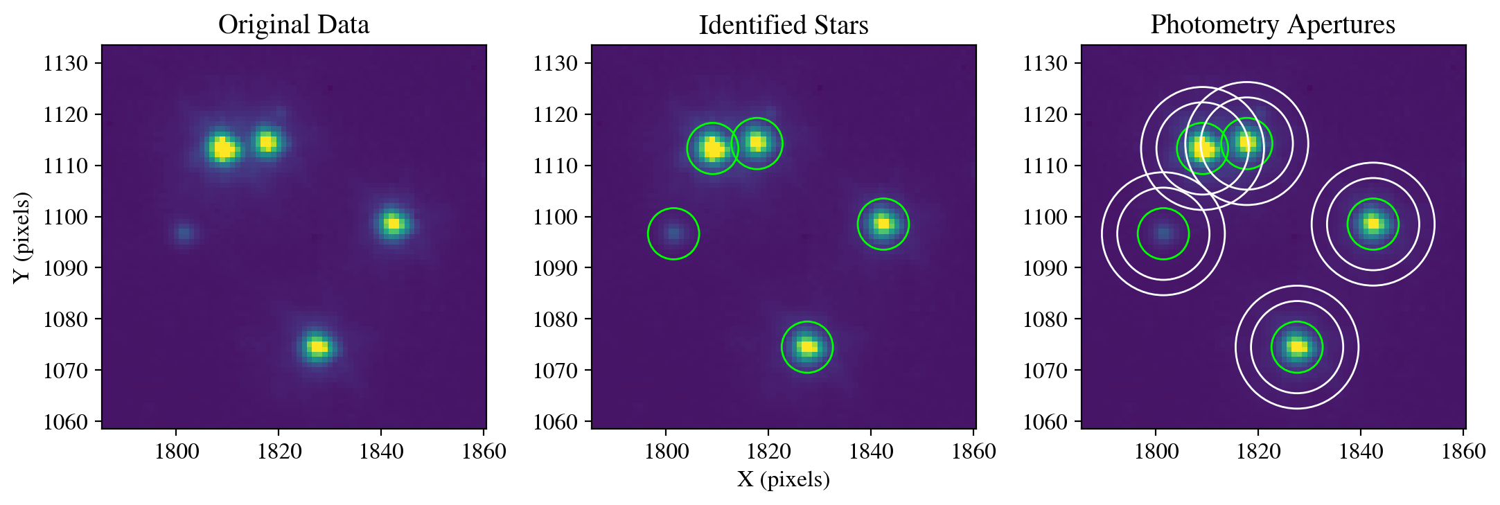
Figure saved as: /home/runner/work/hst_notebooks/hst_notebooks/notebooks/WFC3/point_spread_function/plot/fig11_aperture_photometry.pdf

Finally, we use the stacked model from the drizzled image to perform a PSF fit and subtraction of the same stars examined earlier, with the addition of a faint fifth star on the left of the image. Overall, the model accurately encapsulates the total flux of each star, but some artifacts remain because drizzled images resample the observations.

driz_stack_psf = FittableImageModel(driz_stack[0])
photometry, psfphot = calculate_photometry(sci_driz, sources, psf_model=driz_stack_psf)
resid = psfphot.make_residual_image(sci_driz, (17, 17))
figure = plot_psf_results(sci_driz, resid, 1823, 1096, cutout_size)
save_figure(figure, plot_dir+'fig12_driz_stack.pdf', True)
calculate_residuals(resid, sources)

PSF Photometry (before subtraction):

 id  x_fit   y_fit  flux_fit  qfit
--- ------- ------- -------- -----
  1 1827.61 1074.44   349.35 0.067
  2 1801.56 1096.64    13.89 0.083
  3 1842.42 1098.52   335.00 0.067
  4 1809.24 1113.34   596.20 0.131
  5 1817.77 1114.26   284.88 0.114

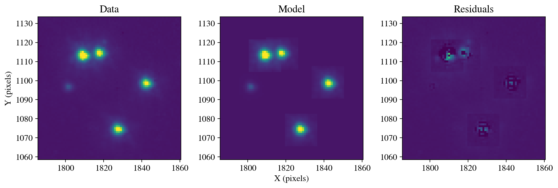
Figure saved as: /home/runner/work/hst_notebooks/hst_notebooks/notebooks/WFC3/point_spread_function/plot/fig12_driz_stack.pdf

Aperture Photometry (after subtraction):

 id xcenter ycenter aperture_sum total_background flux_background_sub
      pix     pix                                                    
--- ------- ------- ------------ ---------------- -------------------
  1 1827.60 1074.49        -4.29             2.66               -6.95
  2 1801.51 1096.62         1.58             0.88                0.70
  3 1842.45 1098.50        -9.13             2.35              -11.48
  4 1809.24 1113.20        16.97             4.73               12.25
  5 1817.78 1114.23        20.33             3.79               16.54 

If users have fewer than approximately 5-10 stars in their drizzled images and cannot create a stacked model, then it is possible to drizzle the empirical models provided by the WFC3 team into FLC files. This requires installing the wfc3_photometry package, running the included make_model_star_image() function within PSFUtils.py on the FLC files, and then extracting and stacking the drizzled models. This functionality is under development and not yet officially supported.

Conclusions

Table of Contents

---

We hope this tutorial provides you with valuable tools and techniques for PSF modeling of HST observations. In summary, we have shown several different workflows for generating PSF models depending on the available observations. First, we demonstrated in Section 2.1 that analytical models such as Gaussian profiles fail to characterize the complex shape of the HST PSF. In Section 2.2, we used empirical models provided by the WFC3 team to accurately characterize the shape of the PSF. We explored using the default models, as well as those modified to match the focus of specific observations, and characterize spatial variations of the PSF across the detector. These models provide high-accuracy astrometry and photometry of stellar sources, but do not account for extended wing emission or diffraction spikes. We tackled this issue in Section 2.3 by stacking stars extracted from the observations, or by retrieving cutouts from MAST. Stacking a large number of sources allows for efficient outlier rejection and can produce a high quality PSF that extends to large radii, but can also broaden the PSF core depending on how the sources are aligned. Finally, we extended this process to drizzled images in Section 3. In some cases, more than one workflow is possible for a given set of observations, and users are encouraged to experiment with these tools to develop the best PSF models for their science goals.

About this Notebook

Table of Contents

---

Author: Mitchell Revalski
Created: 15 Apr 2024
Updated: 05 Jun 2024
Source: spacetelescope/hst_notebooks

Additional Resources

Below are some additional resources that may be helpful. Please send any questions to the HST Help Desk.

• WFC3 Website

• WFC3 PSF Webpage

• WFC3 Data Handbook

• WFC3 Instrument Handbook

• WFC3 Software Tools Webpage

• Introduction to PSF photometry

• HST PSF: Anderson & King (2000)

Software Citations

If you use Python packages such as astropy, astroquery, drizzlepac, matplotlib, or numpy for published research, please cite the authors. Follow the links below for more information about citing various packages:

• Citing astropy

• Citing astroquery

• Citing drizzlepac

• Citing matplotlib

• Citing numpy

• Citing photutils

---

Top of Page