
What to do when you get an Exception Report for COS#
Learning Goals#
This Notebook is designed to walk the user (you) through: investigating the cause of a Hubble Space Telescope (HST) Exception Report.
By the end of this tutorial, you will:
Learn how to examine
FITSheaders of your data to reveal issues with observationsInspect your COS data files to determine whether these were negatively impacted, anomalous, and/or degraded
Table of Contents#
1. Inspecting the Exposure Time
2. Reviewing the Signal-to-Noise Ratio
3. Investigating the Target Acquisition
4. Evaluating the Wavelength Scale
- 5.1 Inspecting the JIF Headers for Guiding Issues
0. Introduction#
The Cosmic Origins Spectrograph (COS) is an ultraviolet spectrograph onboard the Hubble Space Telescope (HST) with capabilities in the near ultraviolet (NUV) and far-ultraviolet (FUV).
This tutorial aims to help you take the appropriate steps after you have received an exception report on your HST/COS observation. An exception report is generated when conditions are present that may have lead to a degredation in data quality, such as an acquisition failure or loss of lock during guiding. When this happens, you receive an email that describes what issues may have occurred during your observations and suggests initial steps to evaluating the quality of your data. The COS Exception Report Instructions webpage suggests a few steps to evaluating the quality of your data so that you can determine whether to file a Hubble Observation Problem Report (HOPR); this notebook will show you how to perform these steps on a variety of different examples from previous COS observations. Your data does not necessarily need to fail all of these steps before a HOPR is filed, you just need to show that there was an issue with your exposures.
Please note that we cannot offer a complete and definitive guide to every exception report. This notebook is simply a general guide to help you understand your data and its quality. Additionally, just because you receive an exception report does not mean that there’s a problem with your data, only that it should be evaluated for quality.
Imports#
We will be using multiple libraries to retrieve and analyze data. We will use:
os,shutil,Path.pathlib, andglobto work with our system’s directories and filepathsmatplotlib.pyplotto plot our datanumpyto perform analysis on our dataastroquery.mastto download our COS datasets for the exercisesastropy.io fitsandastropy.table Tableto read the correspondingFITSfilesscipy.optimizeto fit a Gaussian when calculating the radial velocity
We recommend that you create a new conda environment before running this notebook. Check out the COS Setup.ipynb notebook to install conda. Alternatively, you can download the dependencies required to run this notebook by running the terminal command:
pip install -r requirements.txt
After you download the required dependencies, import them by running the next cell:
from astroquery.mast import Observations

from astropy.io import fits
from astropy.table import Table

from matplotlib.patches import Ellipse
import matplotlib.pyplot as plt

import numpy as np
from scipy import optimize

import shutil
import os
from pathlib import Path

import cos_functions as cf

import warnings
from astropy.utils.exceptions import AstropyWarning

# Ignore Astropy warnings
warnings.simplefilter('ignore', category=AstropyWarning)
0.1 Data Download#
We will begin by downloading all of the data for this notebook using astroquery.mast Observations. Details on how to download COS data can be found in our Data Download Notebook. We will be using examples from many different programs, so we will load in a FITS file with an astropy.Table of observations. We will also create a directory to store these files in, called datapath.
# Creating the folder to store our data
datapath = Path("./data/")
os.makedirs(datapath, exist_ok=True)

# Loading in the FITS table with the list of observations
observations = Table.read("./files.fits")

# Downloading the files to our data directory
Observations.download_products(
    observations,
    download_dir=str(datapath)
)
Downloading URL https://mast.stsci.edu/api/v0.1/Download/file?uri=mast:HST/product/leimacm3q_rawtag_a.fits to data/mastDownload/HST/leimacm3q/leimacm3q_rawtag_a.fits ...
[Done]
Downloading URL https://mast.stsci.edu/api/v0.1/Download/file?uri=mast:HST/product/leimacm3q_rawtag_b.fits to data/mastDownload/HST/leimacm3q/leimacm3q_rawtag_b.fits ...
[Done]
Downloading URL https://mast.stsci.edu/api/v0.1/Download/file?uri=mast:HST/product/leimacm3q_x1d.fits to data/mastDownload/HST/leimacm3q/leimacm3q_x1d.fits ...
[Done]
Downloading URL https://mast.stsci.edu/api/v0.1/Download/file?uri=mast:HST/product/lda920hyq_x1d.fits to data/mastDownload/HST/lda920hyq/lda920hyq_x1d.fits ...
[Done]
Downloading URL https://mast.stsci.edu/api/v0.1/Download/file?uri=mast:HST/product/lda920i3q_x1d.fits to data/mastDownload/HST/lda920i3q/lda920i3q_x1d.fits ...
[Done]
Downloading URL https://mast.stsci.edu/api/v0.1/Download/file?uri=mast:HST/product/lda920iaq_x1d.fits to data/mastDownload/HST/lda920iaq/lda920iaq_x1d.fits ...
[Done]
Downloading URL https://mast.stsci.edu/api/v0.1/Download/file?uri=mast:HST/product/lda920iwq_x1d.fits to data/mastDownload/HST/lda920iwq/lda920iwq_x1d.fits ...
[Done]
Downloading URL https://mast.stsci.edu/api/v0.1/Download/file?uri=mast:HST/product/lda920020_x1dsum.fits to data/mastDownload/HST/lda920020/lda920020_x1dsum.fits ...
[Done]
Downloading URL https://mast.stsci.edu/api/v0.1/Download/file?uri=mast:HST/product/ldy305rkq_x1d.fits to data/mastDownload/HST/ldy305rkq/ldy305rkq_x1d.fits ...
[Done]
Downloading URL https://mast.stsci.edu/api/v0.1/Download/file?uri=mast:HST/product/ldy305rbq_x1d.fits to data/mastDownload/HST/ldy305rbq/ldy305rbq_x1d.fits ...
[Done]
Downloading URL https://mast.stsci.edu/api/v0.1/Download/file?uri=mast:HST/product/ldy305r8q_x1d.fits to data/mastDownload/HST/ldy305r8q/ldy305r8q_x1d.fits ...
[Done]
Downloading URL https://mast.stsci.edu/api/v0.1/Download/file?uri=mast:HST/product/ldy305rpq_x1d.fits to data/mastDownload/HST/ldy305rpq/ldy305rpq_x1d.fits ...
[Done]
Downloading URL https://mast.stsci.edu/api/v0.1/Download/file?uri=mast:HST/product/ldy305010_x1dsum.fits to data/mastDownload/HST/ldy305010/ldy305010_x1dsum.fits ...
[Done]
Downloading URL https://mast.stsci.edu/api/v0.1/Download/file?uri=mast:HST/product/ldc0c0k0q_rawacq.fits to data/mastDownload/HST/ldc0c0k0q/ldc0c0k0q_rawacq.fits ...
[Done]
Downloading URL https://mast.stsci.edu/api/v0.1/Download/file?uri=mast:HST/product/laaf2agfq_rawacq.fits to data/mastDownload/HST/laaf2agfq/laaf2agfq_rawacq.fits ...
[Done]
Downloading URL https://mast.stsci.edu/api/v0.1/Download/file?uri=mast:HST/product/leo906g6q_rawacq.fits to data/mastDownload/HST/leo906g6q/leo906g6q_rawacq.fits ...
[Done]
Downloading URL https://mast.stsci.edu/api/v0.1/Download/file?uri=mast:HST/product/leo906g4q_rawacq.fits to data/mastDownload/HST/leo906g4q/leo906g4q_rawacq.fits ...
[Done]
Downloading URL https://mast.stsci.edu/api/v0.1/Download/file?uri=mast:HST/product/lekcl2seq_rawacq.fits to data/mastDownload/HST/lekcl2seq/lekcl2seq_rawacq.fits ...
[Done]
Downloading URL https://mast.stsci.edu/api/v0.1/Download/file?uri=mast:HST/product/lekcl2sdq_rawacq.fits to data/mastDownload/HST/lekcl2sdq/lekcl2sdq_rawacq.fits ...
[Done]
Downloading URL https://mast.stsci.edu/api/v0.1/Download/file?uri=mast:HST/product/lbhx1cn4q_rawacq.fits to data/mastDownload/HST/lbhx1cn4q/lbhx1cn4q_rawacq.fits ...
[Done]
Downloading URL https://mast.stsci.edu/api/v0.1/Download/file?uri=mast:HST/product/lbs304n1q_rawacq.fits to data/mastDownload/HST/lbs304n1q/lbs304n1q_rawacq.fits ...
[Done]
Downloading URL https://mast.stsci.edu/api/v0.1/Download/file?uri=mast:HST/product/le9i4d020_x1dsum.fits to data/mastDownload/HST/le9i4d020/le9i4d020_x1dsum.fits ...
[Done]
Downloading URL https://mast.stsci.edu/api/v0.1/Download/file?uri=mast:HST/product/le2t09010_jif.fits to data/mastDownload/HST/le2t09010/le2t09010_jif.fits ...
[Done]
Downloading URL https://mast.stsci.edu/api/v0.1/Download/file?uri=mast:HST/product/le2t09010_jit.fits to data/mastDownload/HST/le2t09010/le2t09010_jit.fits ...
[Done]
Downloading URL https://mast.stsci.edu/api/v0.1/Download/file?uri=mast:HST/product/le3a01010_jit.fits to data/mastDownload/HST/le3a01010/le3a01010_jit.fits ...
[Done]
Downloading URL https://mast.stsci.edu/api/v0.1/Download/file?uri=mast:HST/product/le4s04d7j_jif.fits to data/mastDownload/HST/le4s04d7q/le4s04d7j_jif.fits ...
[Done]
Downloading URL https://mast.stsci.edu/api/v0.1/Download/file?uri=mast:HST/product/ldi707tcq_rawtag_a.fits to data/mastDownload/HST/ldi707tcq/ldi707tcq_rawtag_a.fits ...
[Done]
Downloading URL https://mast.stsci.edu/api/v0.1/Download/file?uri=mast:HST/product/ldi707tcq_rawtag_b.fits to data/mastDownload/HST/ldi707tcq/ldi707tcq_rawtag_b.fits ...
[Done]
Downloading URL https://mast.stsci.edu/api/v0.1/Download/file?uri=mast:HST/product/ldi707tcq_x1d.fits to data/mastDownload/HST/ldi707tcq/ldi707tcq_x1d.fits ...
[Done]
| Local Path | Status | Message | URL |
|---|---|---|---|
| str55 | str8 | object | object |
| data/mastDownload/HST/leimacm3q/leimacm3q_rawtag_a.fits | COMPLETE | None | None |
| data/mastDownload/HST/leimacm3q/leimacm3q_rawtag_b.fits | COMPLETE | None | None |
| data/mastDownload/HST/leimacm3q/leimacm3q_x1d.fits | COMPLETE | None | None |
| data/mastDownload/HST/lda920hyq/lda920hyq_x1d.fits | COMPLETE | None | None |
| data/mastDownload/HST/lda920i3q/lda920i3q_x1d.fits | COMPLETE | None | None |
| data/mastDownload/HST/lda920iaq/lda920iaq_x1d.fits | COMPLETE | None | None |
| data/mastDownload/HST/lda920iwq/lda920iwq_x1d.fits | COMPLETE | None | None |
| data/mastDownload/HST/lda920020/lda920020_x1dsum.fits | COMPLETE | None | None |
| data/mastDownload/HST/ldy305rkq/ldy305rkq_x1d.fits | COMPLETE | None | None |
| ... | ... | ... | ... |
| data/mastDownload/HST/lbhx1cn4q/lbhx1cn4q_rawacq.fits | COMPLETE | None | None |
| data/mastDownload/HST/lbs304n1q/lbs304n1q_rawacq.fits | COMPLETE | None | None |
| data/mastDownload/HST/le9i4d020/le9i4d020_x1dsum.fits | COMPLETE | None | None |
| data/mastDownload/HST/le2t09010/le2t09010_jif.fits | COMPLETE | None | None |
| data/mastDownload/HST/le2t09010/le2t09010_jit.fits | COMPLETE | None | None |
| data/mastDownload/HST/le3a01010/le3a01010_jit.fits | COMPLETE | None | None |
| data/mastDownload/HST/le4s04d7q/le4s04d7j_jif.fits | COMPLETE | None | None |
| data/mastDownload/HST/ldi707tcq/ldi707tcq_rawtag_a.fits | COMPLETE | None | None |
| data/mastDownload/HST/ldi707tcq/ldi707tcq_rawtag_b.fits | COMPLETE | None | None |
| data/mastDownload/HST/ldi707tcq/ldi707tcq_x1d.fits | COMPLETE | None | None |
The function, Observations.download_products creates the nested directories ./data/mastDownload/HST/<ROOTNAME>. Run the next cell to move all files from that path to ./data:
mast_path = datapath / Path("mastDownload/HST/")

try:
    for obs_id_path in mast_path.iterdir():
        for file in obs_id_path.glob("*fits"):
            shutil.move(str(file), datapath / file.name)

    shutil.rmtree(mast_path.parent)

except Exception as e:
    print(f"An error occurred: {e}")
1. Inspecting the Exposure Time#
The actual exposure time can indicate issues that may have happened during the observations. If the shutter is closed, then the exposure time will be zero seconds. Additionally, if the actual exposure time is <80% of the planned exposure time, then that is another indicator that there may have been an issue during your observation (see COS ISR 2024-01).
We will define a function below that can give some brief diagnostic information about the exposure time:
def print_exposure_summary(file):
    '''
    Print a summary of the observation, including actual/planned exptime.
    ----------
    Input:
    str or Path file : Path to the RAWTAG file
    ----------
    Output:
    Printed exposure summary.
    '''
    with fits.open(file) as hdul:

        head0 = hdul[0].header
        head1 = hdul[1].header

        print(f'EXPOSURE SUMMARY FOR {head0["FILENAME"]}:')
        print(f'Grating: {head0["OPT_ELEM"]}')
        print(f'Cenwave: {head0["CENWAVE"]}')
        print(f'FPPOS: {head0["FPPOS"]}')
        print(f'Lifetime Position: {head0["LIFE_ADJ"]}')
        print(f'Detector: {head0["DETECTOR"]}')
        print(f'Aperture: {head0["APERTURE"]}')
        print(f'Target Name: {head0["TARGNAME"]}')
        print(f'Target Description: {head0["TARDESCR"]}')
        print(f'Extended?: {head0["EXTENDED"]}')

        if head0["MTFLAG"] == "":
            print('Moving Target?: F')
        else:
            print(f'Moving Target?: {head0["MTFLAG"]}')

        print(f'Visit: {head0["OBSET_ID"]}')
        print(f'ASN ID: {head0["ASN_ID"]}')

        print("---------------")

        print(f'Actual Exptime: {head1["EXPTIME"]}')
        print(f'Planned Exptime: {head1["PLANTIME"]}')
        print(f'Exposure Flag: {head1["EXPFLAG"]}')
        print(f'Shutter: {head0["SHUTTER"]}')
        print(f'Fine guiding lock: {head1["FGSLOCK"]}')

        print("===============")
You will want to pay attention to the actual exposure time (EXPTIME in the secondary header) and the planned exposure time (PLANTIME, also in the secondary header). If the actual exposure time is less than 80% of the planned exposure time, then there was likely an issue with your observations and you may qualify for a repeated observation.
Additional header keywords in the RAWTAG or X1D files to look for are the exposure flag (EXPFLAG, secondary header) which should be NORMAL, the shutter status (SHUTTER in the primary header) which should be OPEN, and the fine-guiding lock keyword (FGSLOCK in the secondary header – more information is in the jitter section of this notebook) which should ideally be FINE (meaning the guide-star tracking was locked).
Let’s examine the header of a successful exposure:
successful_raw_a = datapath / "ldi707tcq_rawtag_a.fits"
successful_raw_b = datapath / "ldi707tcq_rawtag_b.fits"
successful_x1d = datapath / "ldi707tcq_x1d.fits"

print_exposure_summary(successful_raw_a)
EXPOSURE SUMMARY FOR ldi707tcq_rawtag_a.fits:
Grating: G130M
Cenwave: 1291
FPPOS: 4
Lifetime Position: 4
Detector: FUV
Aperture: PSA
Target Name: KNOT-A
Target Description: EXT-CLUSTER;EMISSION LINE NEBULA;MULTIPLE NUCLEI;NUCLEUS;STAR FO
Extended?: YES
Moving Target?: F
Visit: 07
ASN ID: LDI707030
---------------
Actual Exptime: 505.0
Planned Exptime: 505.0
Exposure Flag: NORMAL
Shutter: Open
Fine guiding lock: FINE
===============
We can see that the actual and planned exposure times are the same, the shutter is open, and there weren’t any apparent issues with guide-star tracking. Let’s plot the data below:
fig, ax = plt.subplots(2, 2, figsize=(12, 10))

with fits.open(successful_x1d) as hdul:
    data = hdul[1].data
    flux = data["FLUX"].ravel()
    wl = data["WAVELENGTH"].ravel()

for i, axis in enumerate(ax[0]):
    # Plotting flux vs wavelength on top row
    axis.plot(wl, flux,
              lw=2,
              color="black")

    axis.set_xlabel(r'Wavelength [$\AA$]')
    axis.set_ylabel(r'Flux [$erg\ s^{-1}\ cm^{-2}\ \AA^{-1}$]')

    if i == 0:
        axis.set_title("Flux vs Wavelength")

    else:
        axis.set_title("Flux vs Wavelength, ZOOMED")
        axis.set_ylim(0, 0.6e-13)

for i, axis in enumerate(ax[1]):
    # Plotting the counts on the detector for bottom row
    with fits.open([successful_raw_a, successful_raw_b][i]) as hdul:
        data = hdul[1].data
        axis.scatter(
            data["RAWX"],
            data["RAWY"],
            s=1,
            color=["red", "blue"][i],
            alpha=0.05
        )

    axis.set_xlabel("RAWX")
    axis.set_ylabel("RAWY")

    if i == 0:
        axis.set_title("RAWY vs RAWX, FUVA")

    else:
        axis.set_title("RAWY vs RAWX, FUVB")

plt.suptitle(f'Successful Exposure, {fits.getval(successful_x1d, "ROOTNAME")}',
             fontweight="bold",
             fontsize=15)

plt.tight_layout()

plt.show()
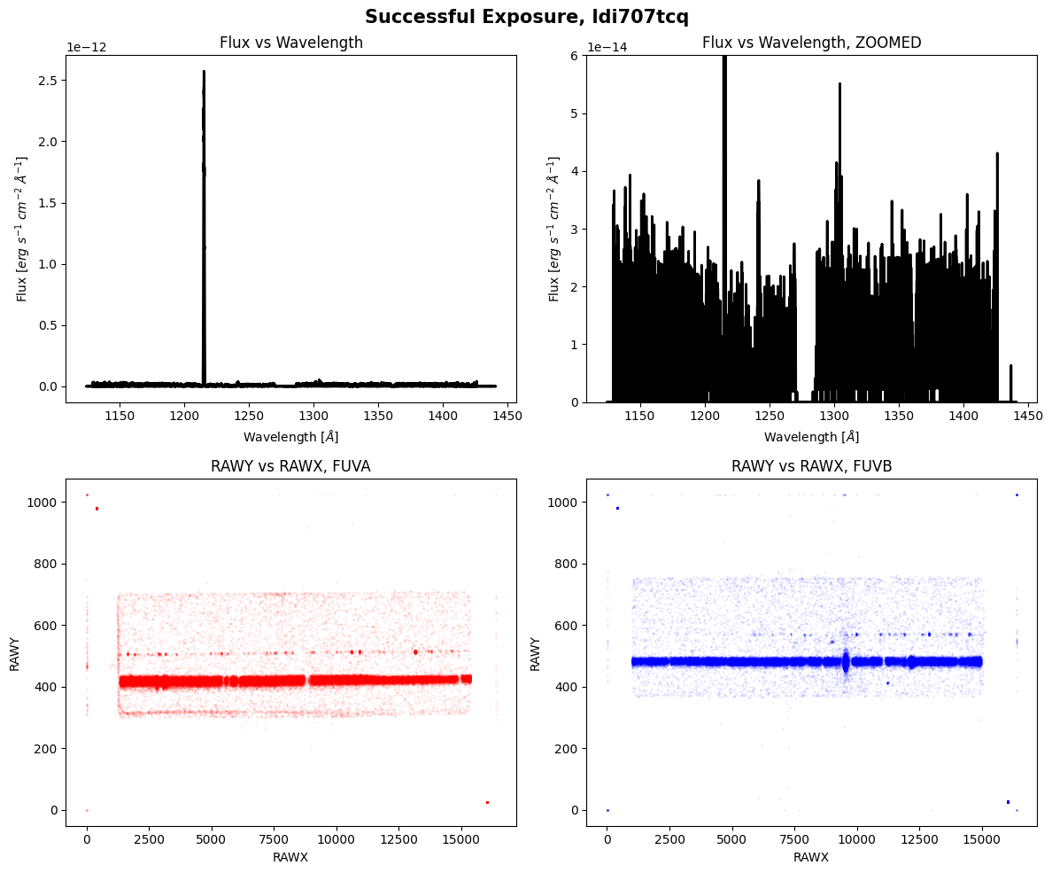
We can clearly see the spectrum and counts landing on both segments of the detectors.
We will plot another exposure in this visit that failed:
failed_raw_a = datapath / "leimacm3q_rawtag_a.fits"
failed_raw_b = datapath / "leimacm3q_rawtag_b.fits"
failed_x1d = datapath / "leimacm3q_x1d.fits"

print_exposure_summary(failed_raw_a)
EXPOSURE SUMMARY FOR leimacm3q_rawtag_a.fits:
Grating: G130M
Cenwave: 1291
FPPOS: 4
Lifetime Position: 4
Detector: FUV
Aperture: PSA
Target Name: SZ66
Target Description: STAR;T TAURI STAR;PRE-MAIN SEQUENCE STAR
Extended?: NO
Moving Target?: F
Visit: AC
ASN ID: LEIMAC010
---------------
Actual Exptime: 0.0
Planned Exptime: 2471.0
Exposure Flag: NO DATA
Shutter: Closed
Fine guiding lock: FINE
===============
We can see that the actual exposure time is zero seconds, the shutter was closed, and the exposure flag has the value NO DATA. We will try to plot the data below, but observations with exposure times of zero cannot carry any actual information, so we will see blank plots:
fig, ax = plt.subplots(2, 2, figsize=(12, 10))

with fits.open(failed_x1d) as hdul:
    data = hdul[1].data
    flux = data["FLUX"].ravel()
    wl = data["WAVELENGTH"].ravel()

for i, axis in enumerate(ax[0]):
    # Plotting flux vs wavelength on top row
    axis.plot(wl, flux,
              lw=2,
              color="black")

    axis.set_xlabel(r'Wavelength [$\AA$]')
    axis.set_ylabel(r'Flux [$erg\ s^{-1}\ cm^{-2}\ \AA^{-1}$]')

    if i == 0:
        axis.set_title("Flux vs Wavelength")

    else:
        axis.set_title("Flux vs Wavelength, ZOOMED")
        axis.set_ylim(0, 1.5e-14)

# Plotting the counts on the detector for bottom row
with fits.open(failed_raw_a) as hdul:
    data = hdul[1].data
    ax[1][0].scatter(
        data["RAWX"],
        data["RAWY"],
        s=1,
        color="red"
    )

for i, axis in enumerate(ax[1]):
    # Plotting the counts on the detector for bottom row
    with fits.open([failed_raw_a, failed_raw_b][i]) as hdul:
        data = hdul[1].data
        axis.scatter(
            data["RAWX"],
            data["RAWY"],
            s=1,
            color=["red", "blue"][i],
            alpha=0.05
        )

    axis.set_xlabel("RAWX")
    axis.set_ylabel("RAWY")

    if i == 0:
        axis.set_title("RAWY vs RAWX, FUVA")

    else:
        axis.set_title("RAWY vs RAWX, FUVB")

plt.suptitle(f'Failed Exposure, {fits.getval(failed_x1d, "ROOTNAME")}',
             fontweight="bold",
             fontsize=15)

plt.tight_layout()

plt.show()
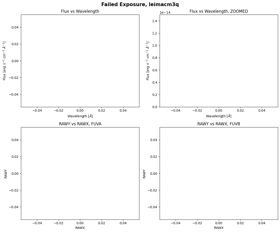
As expected, there is no data to plot.
2. Reviewing the Signal-to-Noise Ratio#
You will want to review the X1DSUM and constituent X1D files for your observation to see if any of the X1D files have dramatically lower (or zero) counts compared to the other X1D files. If the signal-to-noise ratio (SNR) of your X1DSUM file is sufficient for your science even with the problematic X1D, the COS team recommends that you file a Hubble Observation Problem Report (HOPR) and note that you are not requesting a repeat of the observation. This is so the observation is flagged in MAST for potential future investigators.
COS is a photon-counting instrument, so SNR calculations can be simplified compared to other instruments. Information about calculating the SNR of COS data can be found in Chapter 7.3 of the COS Instrument Handbook. The SNR is directly proportional to the square-root of the exposure time. In the COS notebook on Viewing COS Data, we use a simplified equation for the SNR:
This equation is a simplification, and may not be ideal for all datasets. We will plot the SNR for a good observation, and an observation with failed exposures. We will use the cos_functions.py file from the Viewing COS Data Notebook to bin the data to a given resolution element (also known as resel).
We will begin by plotting an example of an X1DSUM and its constituent X1D files with no issues in any of the exposures:
def plot_snr(filelist, quality):
    '''
    Plot the SNR of the X1D files and the X1DSUM.
    SNR is calculated using simplified equation:
        SNR = sqrt(GCOUNTS)
    ----------
    Input:
    [str] filelist : A list of the x1d/x1dsum filepaths for an observation
    str quality : Is this a good or bad observation? Just used in title.
    ----------
    Output:
    SNR is plotted.
    '''
    plt.Figure(figsize=(12, 10))

    for file in sorted(filelist):
        with fits.open(file) as hdul:
            if "x1dsum" in file:
                exptime = hdul[1].header["EXPTIME"]
                label = f"X1DSUM - {exptime} sec"

            else:
                fppos = hdul[0].header["FPPOS"]
                exptime = hdul[1].header["EXPTIME"]
                rootname = hdul[0].header["ROOTNAME"]

                label = f"{rootname}, FPPOS {fppos} - {exptime} sec"

        tab = Table.read(file)
        wavelength = tab["WAVELENGTH"].ravel()

        snr_est = cf.estimate_snr(
            tab,
            verbose=False,
            bin_data_first=True,
            weighted=True,
        )

        plt.plot(np.concatenate([snr_est[1][1][0], snr_est[1][0][0]], axis=0),
                 np.concatenate([snr_est[1][1][1], snr_est[1][0][1]], axis=0),
                 label=label,
                 lw=1,
                 alpha=0.6)

    if quality == "Bad":
        plt.hlines(8, min(wavelength), max(wavelength),
                   linestyles="--",
                   colors="red",
                   label="Required SNR from Phase II")

        plt.ylim(0, 15)

    plt.ylabel("SNR")
    plt.xlabel("Wavelength")
    plt.title(f"SNR vs Wavelength, {quality} Observation")
    plt.legend()
    plt.show()
filelist = [str(file) for file in datapath.glob("*lda920*")]
plot_snr(filelist, "Good")
function `bin_by_resel` is binning by 6
function `bin_by_resel` is binning by 6
function `bin_by_resel` is binning by 6
function `bin_by_resel` is binning by 6
function `bin_by_resel` is binning by 6
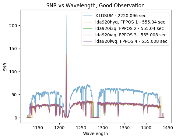
The SNR of the combined X1DSUM file is roughly twice that of the individual X1D files. This is expected because the X1DSUM file is the coadd of the four X1D files, and SNR scales by \(\sqrt{Counts} \propto \sqrt{Exposure\ Time}\). This program requires that the combined SNR be greater than 30, and we can see that this requirement has been satisfied as the X1DSUM SNR is ~50. There likely was not an issue with any of the individual exposures because the SNR of all X1D files is roughly the same.
Let’s plot a problematic observation now. This visit suffered from issues with the guide-star acquisition.
filelist = [str(file) for file in datapath.glob("*ldy305*")]
plot_snr(filelist, "Bad")
function `bin_by_resel` is binning by 6
function `bin_by_resel` is binning by 6
function `bin_by_resel` is binning by 6
function `bin_by_resel` is binning by 6
function `bin_by_resel` is binning by 6
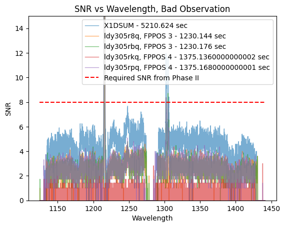
In their Phase II, the PI requires a SNR of at least 8 at 1250Å to accurately do their science. We can see that the SNR of the X1DSUM is around 6, therefore not meeting the science requirement. One of the observations taken at FPPOS 4 (ldy305rkq) has a SNR of almost zero, thus that observation does not add much signal (if any) to the SNR of the X1DSUM file.
3. Investigating the Target Acquisition#
Proper centering of the target within the COS aperture is essential for high-quality data. The COS team recommends for almost all cases that users utilize at least one form of target acquisitions to center the target; a target acquisition is required at least once per visit. More information on target acquisitions can be found in Chapter 8.1 of the COS Instrument Handbook.
There are four different target acquisition modes for COS:
Type of Acquisition |
Steps |
Notes |
|---|---|---|
The instrument moves in a spiral pattern to cover a grid from |
A single |
|
The COS NUV detector takes an image of the target field, moves the telescope to center the target, and then takes an additional NUV image to confirm centering. This is the typical means of target acquisition for COS. |
When using the PSA for the acquisition, users should aim for a |
|
For NUV |
For both NUV and FUV |
|
This algorithm works similarly to |
This acquisition always happens after |
We can analyze the quality of the target acquisition for an observation by looking at the RAWACQ files. We will go through a few examples of evaluating the acquisition for some of these modes. More information about evaluating target acquisitions can be found in Chapter 5.2 of the COS Data Handbook and in COS ISR 2010-14.
3.1 ACQ/SEARCH#
As mentioned above, using the ACQ/SEARCH method for centering moves the instrument N steps in a spiral pattern and calculates the centroid of the target by analyzing the counts at each of these steps (also known as a dwell-point). The RAWACQ file of an ACQ/SEARCH acquisition will contain a header and a binary data table with four different columns, and N*N number of rows, one for each dwell point. The columns DISP_OFFSET and XDISP_OFFSET correspond to the X and Y locations of the specific dwell point, in arcseconds, relative to the initial pointing position. The COUNTS column is the number of counts for that dwell point. To check if you have a successful ACQ/SEARCH acquisition, you can plot the counts of each dwell point and compare the dwell point with the maximum number of counts to the commanded slew position. The coordinates for the commanded slew position are in the header of the RAWACQ file, in the keywords ACQSLEWX and ACQSLEWY.
We will define a function to plot the ACQ/SEARCH table, and we will plot the table of a successful and unsuccessful acquisition.
def plot_acq_search(file):
    '''
    Plot the ACQ/SEARCH table, to help assess acquisition data quality.
    The commanded slew and the dwell point with highest counts should be
    the same for a successful acquisition.
    ----------
    Input:
    str or Path file : Path to the ACQ/SEARCH exposure.
    ----------
    Output:
    Plot with counts at each dwell point for the exposure.
    Commanded slew point is also plotted.
    '''
    # Reading in the file's data
    data = Table.read(file)

    # The unique dwell points in DISP/XDISP grid
    disp_unique = np.unique(data["DISP_OFFSET"])
    xdisp_unique = np.unique(data["XDISP_OFFSET"])

    # Empty table for dwell points' counts
    dwell_table = np.zeros((len(disp_unique), len(xdisp_unique)))

    # Filling the table with count values
    for row in data:

        # Getting the index for the grid
        i_disp = np.where(disp_unique == row["DISP_OFFSET"])[0][0]
        i_xdisp = np.where(xdisp_unique == row["XDISP_OFFSET"])[0][0]

        # Adding counts value to grid location
        dwell_table[i_disp, i_xdisp] = row["COUNTS"]

    # For the plot:
    # The "bounding box" of image, plus a little extra so nothing is cut off
    # In form (LEFT, RIGHT,
    #          BOTTOM, TOP)
    box = (disp_unique[0]-0.5, disp_unique[-1]+0.5,
           xdisp_unique[0]-0.5, xdisp_unique[-1]+0.5)

    plt.figure(figsize=(10, 8))

    # Plotting the dwell point grid
    plt.imshow(
        dwell_table,
        origin="lower",
        aspect="auto",
        extent=box
    )

    plt.colorbar(label="Counts")

    # Getting coordinates for commanded slew
    xslew = fits.getval(file, "ACQSLEWX")
    yslew = fits.getval(file, "ACQSLEWY")

    # Putting commanded slew position on plot
    plt.scatter(
        xslew,
        yslew,
        label="Commanded Slew Location",
        marker="*",
        color="red",
        s=250
    )

    # Adding formatting
    plt.xlabel("DISP_OFFSET (arcsec)")
    plt.ylabel("XDISP_OFFSET (arcsec)")

    scansize = fits.getval(file, "SCANSIZE")

    plt.title(f'ACQ/SEARCH of {fits.getval(file, "ROOTNAME")}, SCAN-SIZE = {scansize}',
              fontweight="bold")

    plt.grid(False)
    plt.legend()

    plt.show()
Let’s plot a successful target acquisition:
plot_acq_search(datapath / "ldc0c0k0q_rawacq.fits")

As we can see above, the dwell point with the maximum counts is not at the edge of the scan area, and the commanded slew is consistent with the dwell point with the highest counts.
An example of a failed ACQ/SEARCH acquisition can be seen below. For this observation, there was an issue with the guide-star acquisition, and the COS shutter closed as a result.
plot_acq_search(datapath / "laaf2agfq_rawacq.fits")
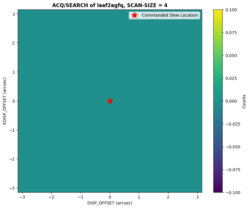
We can see in the plot above that the counts across the whole scan are zero, which is expected since the shutter was closed for the acquisition.
3.2 ACQ/IMAGE#
For an ACQ/IMAGE acquisition, two images are taken with the NUV detector. The first one is taken after the initial HST pointing. The flight software calculates the movement needed to center the object to the center of the aperture, centers the object, and then takes a confirmation image. The initial and confirmation images can be found in the ACQ/IMAGE RAWACQ file. There are a total of six images (and one primary header) in the FITS file. Three for the initial image (one is the image, another is ERR and the third is DQ flagged data), and three for the confirmation image (ERR and DQ).
def plot_acq_image(file):
    '''
    Plot the initial and confirmation acquisition image of an ACQ/IMAGE _rawacq
    file. The expected and measured centroids of the target are also plotted.
    ----------
    Input:
    str or Path peakd : Path to the ACQ/IMAGE exposure.
    ----------
    Output:
    Initial and confirmation image are plotted with a colorbar and expected/measured centroids.
    '''
    fig, (initial, confirm) = plt.subplots(2, 1, figsize=(10, 10), sharex=True)

    with fits.open(file) as hdul:
        header = hdul[0].header

        print(f'Exposure time for initial image: {hdul[1].header["EXPTIME"]} seconds')
        print(f'Exposure time for confirmation image: {hdul[4].header["EXPTIME"]} seconds')

        # Plotting the initial image
        initial_im = initial.imshow(hdul[1].data,
                                    vmin=0,
                                    vmax=0.1,
                                    aspect="auto")

        initial.plot(
            header["ACQPREFX"],
            header["ACQPREFY"],
            "*",
            label="Desired Centroid",
            ms=15,
            alpha=0.8,
            color="green"
        )

        initial.plot(
            header["ACQCENTX"],
            header["ACQCENTY"],
            "o",
            label="Initial Centroid",
            ms=10,
            alpha=0.6,
            color="red"
        )

        conf_im = confirm.imshow(hdul[4].data,
                                 vmin=0,
                                 vmax=0.1,
                                 aspect="auto")

        confirm.plot(
            header["ACQCENTX"],
            header["ACQCENTY"],
            "o",
            label="Measured Center",
            ms=10,
            alpha=0.6,
            color="red"
        )

    initial.set_title("Initial Acquisition Image")
    confirm.set_title("Confirmation Acquisition Image")

    title = f'Initial and Confirmation Image for {fits.getval(file, "ROOTNAME")}, ACQ/IMAGE'

    plt.suptitle(title, fontweight="bold")

    fig.colorbar(initial_im, label="Counts")
    fig.colorbar(conf_im, label="Counts")

    initial.legend()
    confirm.legend()

    plt.show()
We will plot a successful ACQ/IMAGE acquisition; we will see the measured flight-software (FSW) centroid in the location of the area of the detector with the highest number of counts (which is the location of the target).
plot_acq_image(datapath / "lbhx1cn4q_rawacq.fits")
Exposure time for initial image: 76.0 seconds
Exposure time for confirmation image: 76.0 seconds

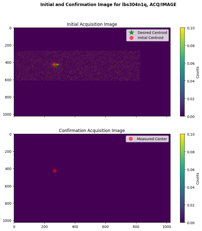
We will also plot an example of a failed ACQ/IMAGE acquisition, where the COS shutter closed before the confirmation acquisition image was taken due to a guide-star acquisition failure.
plot_acq_image(datapath / "lbs304n1q_rawacq.fits")
Exposure time for initial image: 252.0 seconds
Exposure time for confirmation image: 0.0 seconds
3.3 ACQ/PEAKXD, ACQ/PEAKD#
ACQ/PEAKXD and ACQ/PEAKD exposures can be taken after dispersed light acquisitions to further improve the centering of your target. The ACQ/PEAKXD exposure is taken before the ACQ/PEAKD exposure. We can check the quality of these acquisitions in a similar manner as to the ACQ/SEARCH example. Similarly to ACQ/SEARCH files, the ACQ/PEAKD files have data for the dwell points and their respective counts in the Ext 1 header. In a successful exposure, the dwell point with the maximum number of counts is in the center of the scan and the slew offset header keyword (ACQSLEWX) is in this location as well.
We will define a function to plot a ACQ/PEAKXD/ACQ/PEAKD exposure, and then plot an example of a successful exposure.
def plot_peakdxd(peakd, peakxd):
    '''
    Plot the ACQ/PEAKD and ACQ/PEAKXD tables, and mark the zero offset location.
    In a successful exposure, the dwell point with the max counts will be
    at an offset of 0.0.

    ** Note that the vmin and vmax (colorbar scale range) is hardcoded to aid in **
       visualization of the bad data's plot.
    ----------
    Input:
    str or Path peakd : Path to the ACQ/PEAKD exposure.
    str or Path peakxd : Path to the ACQ/PEAKXD exposure.
    ----------
    Output:
    Plot with counts at each dwell point for the exposures.
    '''
    fig, ax = plt.subplots(1, 2, figsize=(12, 8))

    # First is the XD acq
    peakxd_table = Table.read(peakxd)

    cxd = ax[0].scatter(
        peakxd_table["XDISP_OFFSET"],
        peakxd_table["DWELL_POINT"],
        c=peakxd_table["COUNTS"],
        s=2000,
        marker="s",
        cmap="viridis",
        vmin=0,
        vmax=2750
    )

    # Second is the AD acq
    peakd_table = Table.read(peakd)

    cd = ax[1].scatter(
        peakd_table["DISP_OFFSET"],
        peakd_table["DWELL_POINT"],
        c=peakd_table["COUNTS"],
        s=2000,
        marker="s",
        cmap="viridis",
        vmin=0,
        vmax=2750
    )

    for subplot, column in zip(ax, ["XDISP_OFFSET", "DISP_OFFSET"]):

        subplot.set_xlabel(column,
                           fontweight="bold")
        subplot.set_ylabel("DWELL POINT",
                           fontweight="bold")

        subplot.axvline(0, 0, 6,
                        linestyle="dashed",
                        lw=2,
                        color="black",
                        label="Zero Offset")

        subplot.legend(loc="center right")

    cbxd = fig.colorbar(cxd, ax=ax[0])
    cbxd.set_label("Counts",
                   fontweight="bold")

    cbd = fig.colorbar(cd, ax=ax[1])
    cbd.set_label("Counts",
                  fontweight="bold")

    ax[0].set_title(f'PEAKXD for {fits.getval(peakxd, "ROOTNAME")}',
                    fontweight="bold")
    ax[1].set_title(f'PEAKD for {fits.getval(peakd, "ROOTNAME")}',
                    fontweight="bold")

    plt.tight_layout()
    plt.show()
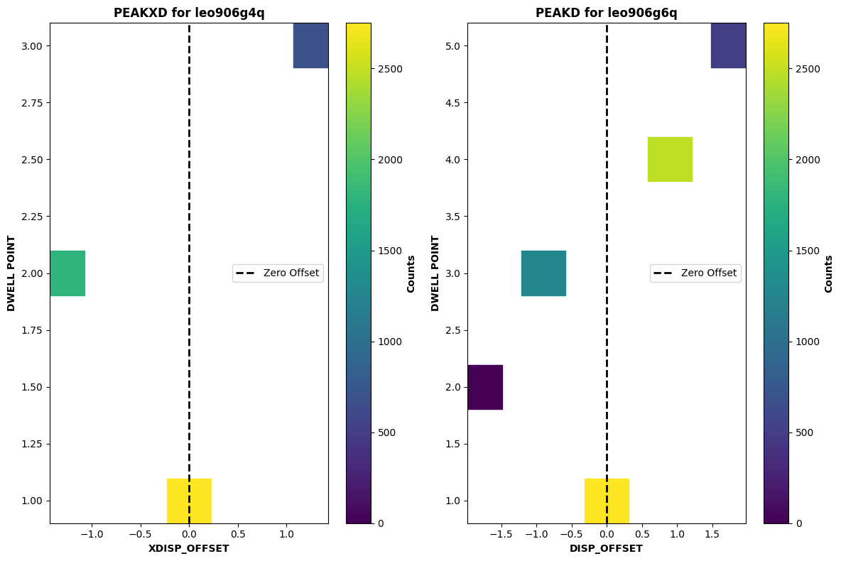
Now we will plot a successful ACQ/PEAKD & ACQ/PEAKXD acquisition using the respective RAWACQ files. Note how the dwell points with the highest number of counts are in the center for both acquisitions.
peakd = datapath / "leo906g6q_rawacq.fits"
peakxd = datapath / "leo906g4q_rawacq.fits"
plot_peakdxd(peakd, peakxd)
And now we will plot an unsuccessful acquisition, where the shutter was closed:
peakd = datapath / "lekcl2seq_rawacq.fits"
peakxd = datapath / "lekcl2sdq_rawacq.fits"
plot_peakdxd(peakd, peakxd)
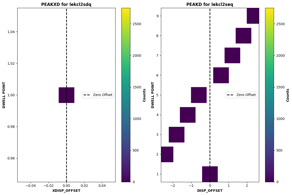
Similar to the ACQ/SEARCH example, we can see that the counts across the entire scan are zero. Since the shutter was closed, there was an issue with the observation.
4. Evaluating the Wavelength Scale#
If your target is not centered well in the aperture, then you can experience issues with the wavelength scale, i.e. there may be an offset in the dispersion direction. The minimum wavelength accuracy for each COS mode is listed in Chapter 8.8 of the COS Instrument Handbook. If a large enough offset is apparent between the observed and expected line positions of your target, then you will want to check the target’s centering.
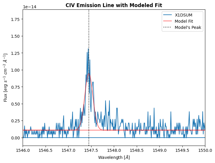
We will go through an example of an observation with a poor wavelength scale. This observation was part of the ULLYSES project, and observed the T-Tauri Star V510-Ori. We will calculate the radial velocity of the target using the CIV lines at 1548.19 Å.
To calculate the radial velocity, we will fit a curve to the CIV line of the X1DSUM G160M file, and compare the peak of this curve with the expected location of the CIV line. We will then use the equation below to calculate the radial velocity:
\( v_r = c \left( \frac{\lambda - \lambda_0}{\lambda_0} \right) \)
Where:
\( v_r \) is the radial velocity,
\( c \) is the speed of light (\( \approx 2.99 * 10^5 \) km/s),
\( \lambda \) is the observed wavelength of the spectral line,
\( \lambda_0 \) is the rest wavelength of the spectral line.
We will first define a function that will fit a Gaussian to our emission line:
def fit_gaussian(wavelength, amplitude, mean, stddev):
    '''
    Fit a Gaussian to the data.
    Gaussian is defined as:
    f(x) = c + amplitude * np.exp(-(((wavelength - mean) / stddev)**2)/2)
    ----------
    Input:
    arr wavelength : Data of the independent variable (wl in our context)
    float amplitude : Amplitude of Gaussian. Represents the peak of the data
    float mean : Mean wl of Gaussian. Represents central wavelength of feature
    float stddev : Standard deviation of Gaussian. Represents function's width
    ----------
    Output:
    The value of flux at each wavelength using the fit.
    '''
    # An estimate of the continuum flux value
    c = 1.1e-15
    return c + amplitude * np.exp(-(((wavelength - mean) / stddev)**2)/2)
We will now use scipy.optimize curve_fit to fit this function to the CIV line of the X1DSUM. We will do our fit between the wavelength range 1546 - 1550 Å.
# Extracting the X1DSUM file's data
with fits.open(datapath / "le9i4d020_x1dsum.fits") as hdul:
    wavelength = hdul[1].data["WAVELENGTH"].ravel()
    flux = hdul[1].data["FLUX"].ravel()

# Getting the indicies within the wavelength range
indicies = np.where((wavelength >= 1546) & (wavelength <= 1550))

trimmed_flux = flux[indicies]
trimmed_wl = wavelength[indicies]

# We need to make an initial guess for the parameter values
# The array is in form [PEAK OF GAUSSIAN, CENTRAL WAVELENGTH, WIDTH OF LINE]
p0 = [1.2e-14, 1547.6, 0.008]

popt, _ = optimize.curve_fit(fit_gaussian,
                             trimmed_wl,
                             trimmed_flux,
                             p0)

print(f"The CIV peak is fitted to be {np.round(popt[1], 3)} Å")

# Plotting the emission feature and our fit
plt.figure(figsize=(8, 6))

# Plotting the actual data
plt.plot(
    wavelength,
    flux,
    label="X1DSUM"
)

# Plotting our fit
plt.plot(
    wavelength,
    fit_gaussian(wavelength, *popt),
    label="Model Fit",
    color="red",
    alpha=0.6
)

# Adding vertical lines to show fitted "peak"
plt.axvline(popt[1],
            label='Model\'s Peak',
            color="black",
            linestyle="dotted")

plt.xlim(1546, 1550)
plt.legend()

plt.xlabel(r'Wavelength [$\AA$]')
plt.ylabel(r'Flux [$erg\ s^{-1}\ cm^{-2}\ \AA^{-1}$]')
plt.title("CIV Emission Line with Modeled Fit",
          fontweight="bold")

plt.show()
The CIV peak is fitted to be 1547.45 Å
We will then use the equation defined earlier to calculate the radial velocity. The rest wavelength for CIV is 1548.19 Å.
# Speed of light (in km/s)
c = 2.99e5

# Getting the observed wavelength of our HLSP
observed_wavelength = popt[1]

# Rest wavelength of CIV
rest_wavelength = 1548.19

v_r = c * ((observed_wavelength - rest_wavelength) / rest_wavelength)
v_r = np.round(v_r, 2)

print(f"The radial velocity of the target is {v_r} km/s")
The radial velocity of the target is -142.97 km/s
The literature value of the radial velocity for this target is ~33.3 km/s. There is a > 150 km/s difference in the radial velocity, which is far above the minimum accuracy of +/- 15 km/s, indicating that there was likely an issue with the target centering during this visit. Since this dataset passed all other data quality checks, the ULLYSES team applied a manual shift which corrected the data.
Note: If your observation has a slight shift, and passes other data quality checks, then you can manually apply a shift to correct your data. Details of this are in Chapter 5.3.2 of the COS Data Handbook, and there is a tutorial in the HASP notebook repository as well.
5. Checking the Jitter#
Jitter is caused by spacecraft motion during the observation. This can be due to a variety of reasons, including micro-meteor impact or a day-night transition. The jitter files contain information about the performance of the Pointing Control System (PCS) and the Fine Guidance Sensors (FGS) during your observation; they are produced by the Engineering Data Processing System (EDPS), which is software that analyzes the HST spacecraft telemetry. There are two relevant jitter files that are produced: one is the JIT table, which is a table that contains 3-second average pointing data, and the JIF file, which is a 2D histogram of the JIT table. These files are produced for all COS science exposures (with the exception of acquisitions). For more information on jitter files, check out Chapter 5.1 of the HST Data Handbook.
We will walk through analyzing the JIF and JIT files for two different datasets: one dataset with a low amount of jitter and one with a high amount of jitter.
5.1 Inspecting the JIF Headers for Guiding Issues#
We can first take a look at the headers of the JIF file, which can provide us with information about the guide-star lock; this information is in the primary header, under the Problem Flags and Warnings section. Additionally, in the secondary header, there is information about the commanding guiding mode. There are three modes, FINE LOCK, FINE LOCK/GYRO, and GYRO. If there was a problem with the observation guiding, then the secondary header keywords, GUIDECMD and GUIDEACT, will not match. These keywords are the “command guiding mode” and the “actual guiding mode”, respectively. If the GUIDEACT keyword value is FINE LOCK/GYRO, or GYRO, then there may have been a problem with the guide-star acquisition and the target may have moved out of the aperture. More information about analyzing these logs is in Chapter 5.2 of the HST Data Handbook.
Below, we will define a function to quickly read the header keywords from the JIF file and determine if there may have been an issue with the guiding. Please note that you will still need to check the jitter table (which we will do later), regardless of any Problem Flags and Warnings that are printed because the information we will print is going to be related to guiding rather than indicative of the actual jitter of the instrument.
def print_jif_headinfo(jiffile):
    '''
    Print important keywords from the JIF file for an observation.
    ----------
    Input:
    Pathlib.path jiffile : Path to the JIF file for your observation
    ----------
    Output:
    Will print out relevant JIF header information, as well as print if there are
    any problem flags or warnings.
    '''
    # A dict of relevant keywords and their vals during a good obs
    jif_keys = {
        "T_GDACT": True,
        "T_ACTGSP": True,
        "T_GSFAIL": False,
        "T_SGSTAR": False,
        "T_TLMPRB": False,
        "T_NOTLM": False,
        "T_NTMGAP": 0,
        "T_TMGAP": 0.000000,
        "T_GSGAP": False,
        "T_SLEWNG": False,
        "T_TDFDWN": False
    }

    # Opening the JIF file to see header info
    with fits.open(jiffile) as hdul:

        head0 = hdul[0].header
        head1 = hdul[1].header

        # An empty list of flags, will contain any deviations from jif_keys
        flags = []

        print(f"Printing JIF information for {head0['FILENAME']}:\n")

        for key, value in jif_keys.items():

            act_val = head0[key]
            print(f"{key} = {head0[key]} / {head0.comments[key]}")

            # Append if there's a mismatch between the normal val and obs val
            if act_val != value:
                flags.append(f"{key} = {head0[key]} / {head0.comments[key]}")

        print("\nGuidings:")

        print(f'GUIDECMD = {head0["GUIDECMD"]} / {head0.comments["GUIDECMD"]}')
        print(f'GUIDEACT = {head1["GUIDEACT"]} / {head1.comments["GUIDEACT"]}')

        if (head0["GUIDECMD"] != head1["GUIDEACT"]) & (len(flags) != 0):
            print("\n===== Warnings from headers: =====\n")

        if head0["GUIDECMD"] != head1["GUIDEACT"]:
            print(f"Mismatch between GUIDECMD and GUIDEACT; \
                  GUIDECMD = {head0['GUIDECMD']} and GUIDEACT = {head1['GUIDEACT']}")

        if len(flags) != 0:
            for flag in flags:
                print(flag)

    return
Let’s print out the JIF header information for a dataset with low jitter. We will see that there are no warnings from the header keyword values, indicating that there was no issue with the guiding during the observation.
print_jif_headinfo(datapath / "le2t09010_jif.fits")
Printing JIF information for le2t09010_jif.fits:

T_GDACT = True / Actual guiding mode same for all exposures
T_ACTGSP = True / Actual Guide Star Separation same in all exps.
T_GSFAIL = False / Guide star acquisition failure in any exposure
T_SGSTAR = False / Failed to single star fine lock
T_TLMPRB = False / problem with the engineering telemetry in any e
T_NOTLM = False / no engineering telemetry available in all exps.
T_NTMGAP = 0 / total number of telemetry gaps in association
T_TMGAP = 0.0 / total duration of missing telemetry in asn. (s)
T_GSGAP = False / missing telemetry during GS acq. in any exp.
T_SLEWNG = False / Slewing occurred during observations
T_TDFDWN = False / Take Data Flag NOT on throughout observations

Guidings:
GUIDECMD = FINE LOCK / Commanded Guiding mode
GUIDEACT = FINE LOCK / Actual Guiding mode at end of GS acquisition
We will now print the header information for the failed example observation used in the ACQ/IMAGE section, which suffered from guide-star issues during the target acquisition.
print_jif_headinfo(datapath / "le4s04d7j_jif.fits")
Printing JIF information for le4s04d7j_jif.fits:

T_GDACT = True / Actual guiding mode same for all exposures
T_ACTGSP = True / Actual Guide Star Separation same in all exps.
T_GSFAIL = True / Guide star acquisition failure in any exposure
T_SGSTAR = False / Failed to single star fine lock
T_TLMPRB = False / problem with the engineering telemetry in any e
T_NOTLM = False / no engineering telemetry available in all exps.
T_NTMGAP = 0 / total number of telemetry gaps in association
T_TMGAP = 0.0 / total duration of missing telemetry in asn. (s)
T_GSGAP = False / missing telemetry during GS acq. in any exp.
T_SLEWNG = False / Slewing occurred during observations
T_TDFDWN = True / Take Data Flag NOT on throughout observations

Guidings:
GUIDECMD = FINE LOCK / Commanded Guiding mode
GUIDEACT = GYRO / Actual Guiding mode at end of GS acquisition

===== Warnings from headers: =====

Mismatch between GUIDECMD and GUIDEACT;                   GUIDECMD = FINE LOCK and GUIDEACT = GYRO
T_GSFAIL = True / Guide star acquisition failure in any exposure
T_TDFDWN = True / Take Data Flag NOT on throughout observations
Since the header keywords GUIDECMD and GUIDEACT are not identical, there was slewing during the observation, and the TDFFLAG went up during the observation, we can conclude that there was an issue with the guiding for this observation.
5.2 Inspecting the JIT Table#
As mentioned earlier, the JIT table contains the pointing data for science observations. For evaluating our jitter, we will look specifically at the SI_V2_AVG and SI_V3_AVG values, which are the mean jitter for a 3-second average at V2 and V3 (two of the HST axes), respectively. The other columns of the JIT table can be found in Table 2.12 of the COS Data Handbook.
We will define a function to make a plot of the SI_V2_AVG and SI_V3_AVG and then plot a high and low jitter example datasets.
def plot_jitter(jit_file, severity="", rss=False, n_sigma=2, n_bins=25):
    '''
    Pathlib.path jit_file : Path to the jitter file
    str severity : How bad is the jitter? Just used in plot title
    bool rss : True if you want to return the RSS. Will not result in plot
    int n_sigma : How many stdevs do you want to visualize?
    int n_bins : Number of bins for the 2D histogram
    ----------
    Output:
    float v2_stdev : Stdev of SI_V2_AVG
    float v3_stdev : Stdev of SI_V3_AVG
    A 2D histogram of the SI_V2_AVG and SI_V3_AVG with an
    elliptical contour with spread of n_sigma.
    '''
    data = Table.read(jit_file, hdu=1)

    v2_avg, v3_avg = data["SI_V2_AVG"], data["SI_V3_AVG"]

    v2_stdev = np.std(v2_avg)
    v3_stdev = np.std(v3_avg)

    if rss:
        return v2_stdev, v3_stdev

    plt.Figure(figsize=(12, 12))

    plt.hist2d(
        x=v2_avg,
        y=v3_avg,
        bins=n_bins
    )

    ax = plt.gca()

    ellipse_center = (np.mean(v2_avg), np.mean(v3_avg))

    ellipse = Ellipse(
        xy=ellipse_center,
        width=n_sigma*v2_stdev,
        height=n_sigma*v3_stdev,
        fill=False,
        lw=2,
        color="red"
    )

    label_x = ellipse_center[0] + n_sigma * v2_stdev / 2
    label_y = ellipse_center[1] + n_sigma * v3_stdev / 2

    ax.text(label_x, label_y,
            f'{n_sigma} sigma contour',
            color='black',
            bbox=dict(facecolor="white",
                      alpha=0.7),
            fontsize=12,
            fontweight="bold")

    ax.add_patch(ellipse)

    plt.title(f"2D Histogram of 3 sec Mean Jitter, {severity}",
              fontweight="bold")

    plt.xlabel(r"SI_V2_AVG [arcsec], $\sigma$="+str(np.round(v2_stdev, 3))+'"')
    plt.ylabel(r"SI_V3_AVG [arcsec], $\sigma$="+str(np.round(v3_stdev, 3))+'"')

    plt.show()

    return
Let’s plot the observation with a low amount of jitter:
low_jit = datapath / "le2t09010_jit.fits"
plot_jitter(low_jit, "Low Amount of Jitter")
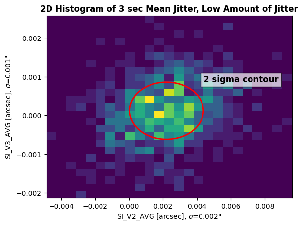
The plot above is a 2D histogram of the mean jitter at V2 and V3. An ellipse is plotted on top of the histogram to visualize two standard deviations from the mean contour. On the X and Y axes is the standard deviation value for SI_V2_AVG and SI_V3_AVG. Ideally, since the throughput of the target’s flux begins to decrease around 0.4" off the center of the aperture (see Chapter 8.8 of the COS Instrument Handbook), the Root-Sum-Square (RSS) of the data should be less than 0.4". The RSS is a statistical measure of uncertainty to combine multiple measurements of uncertainty. It can be calculated with the equation:
\( \text{RSS} = \sqrt{\sigma_X^2 + \sigma_Y^2} \)
Let’s calculate the RSS of the low jitter dataset:
v2_stdev, v3_stdev = plot_jitter(low_jit, rss=True)

rss_low = np.sqrt(v2_stdev**2 + v3_stdev**2)

print(f"The Root-Sum-Square of the low jitter dataset is {np.round(rss_low, 3)}\"")
The Root-Sum-Square of the low jitter dataset is 0.0020000000949949026"
As we can see, the RSS of the low jitter dataset was 0.002", well within the 0.4" centering quality limit.
Let’s take a look at the high jitter dataset:
high_jit = datapath / "le3a01010_jit.fits"

plot_jitter(high_jit, "High Amount of Jitter")
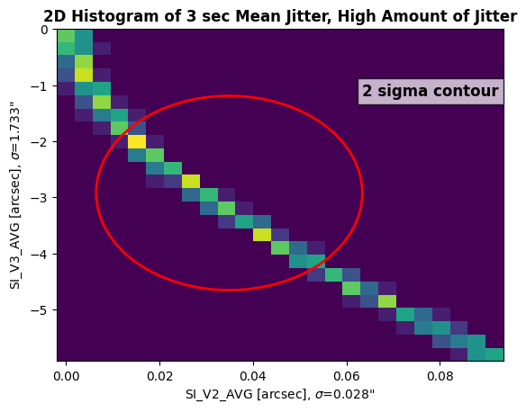
We can see that this dataset looks very different than the low jitter dataset. The spread of the jitter is much greater than our previous example, especially for SI_V3_AVG. We are seeing a large contour, indicating a big spread in jitter values throughout the observation. Let’s calculate the RSS of this data:
v2_stdev, v3_stdev = plot_jitter(high_jit, rss=True)

rss_high = np.sqrt(v2_stdev**2 + v3_stdev**2)

print(f"The Root-Sum-Square of the high jitter dataset is {np.round(rss_high, 3)}\"")
The Root-Sum-Square of the high jitter dataset is 1.7339999675750732"
This observation’s RSS of the jitter values is 1.734", indicating that the target may have gone off center during the course of the observation. In this instance, the user should check for large variations in the count rate throughout the observation (assuming the target is not variable). A tutorial notebook for creating lightcurves with COS data can be found here.
Congrats on completing the notebook!#
There are more tutorial notebooks for COS in this repo, check them out!#
About this Notebook#
Author: Sierra Gomez (sigomez@stsci.edu)
Updated on: August 29, 2024
This tutorial was generated to be in compliance with the STScI style guides and would like to cite the Jupyter guide in particular.
Citations#
If you use astropy, astroquery, or matplotlib, numpy for published research, please cite the authors. Follow these links for more information about citations:
