
Aligning HST Mosaics#
Learning Goals#
By the end of this notebook tutorial, you will:
Download WFC3 UVIS & IR images with
astroqueryCheck the active WCS (world coordinate system) solution in the FITS images
Create a Gaia reference catalog and align the IR images using
TweakRegVerify the quality of the alignment results and compare to the MAST alignment solutions
Update the WCS and use
AstroDrizzleto combine the IR mosaicAlign the UVIS data to the IR drizzled mosaic using
TweakRegUpdate the WCS and use
AstroDrizzleto combine the UVIS mosaic
Table of Contents#
1. Imports
2. MAST Download
3. Check image header data
3.1 IR detector
3.2 UVIS detector
4. Inspect the WCS Solution and fit statistics
5. Create Gaia Catalog
6. TweakReg for Mosaics
6.1 IR Alignment
6.2 Inspect the shift file to verify the pointing residuals
6.3 Inspect the IR fits
7. Mosaicking Features in AstroDrizzle
7.1 Drizzle the IR/F160W Mosaic
7.2 Display the combined DRZ science and weight images
8. Align the UVIS FLC frames to the IR mosaic
8.1 Inspect the shift file to verify the pointing residuals
8.2 Inspect the UVIS fits
9. Drizzling the F657N mosaic
9.1 Display the combined DRC science and weight images
10. Conclusions
Introduction #
This notebook demonstrates how to align and drizzle mosaicked tiles of the Eagle Nebula (M16) obtained with WFC3 with both
UVIS and IR detectors. It is based on the example highlighted in the following WFC3 technical report: ISR 2015-09: Combining
WFC3 Mosaics of M16 with DrizzlePac and highlights special features in DrizzlePac to improve mosaics.
In prior alignment tutorials, building up an aligned set of tiles required an iterative approach. Now, mosaic alignment can be
achieved in a single step by aligning to the Gaia eDR3 reference catalog. We also show how to use sky matching in AstroDrizzle
to produce seamless mosaics, which can be challenging for extended sources with little or no blank sky.
Observations #
Mosaics of the Eagle Nebula were acquired by HST GO/DD program 13926 (PI Z. Levay) in September 2014 for HST’s 25th
Annivery. A 2x2 tile mosaic with the IR detector (~4 arcmin across) was observed in the F110W and F160W filters.
A slightly larger 2x2 mosaic with the UVIS detector (~5 arcmin across) was observed with the F502N, F657N, and F673N filters.
Small dithers between exposures in a given tile will fill in the UVIS chip gap and allow for the rejection of cosmic rays and detector
artifacts. More detail on the observing strategy may be found in the Phase II file.
Two additional UVIS tiles overlap the central portion of 2x2 mosaic in order to increase the high signal-to-noise in the Eagle’s pillars.
These two visits (09,10) are not included in this example for brevity but can be added by the user. The data used in this notebook
example is also limited to a single IR filter (F160W, visits 01-04) and a single UVIS filter (F657N, visits 05-08), shown in the diagrams
below. Additional filters in both detectors are available for this observing program.
 IR Mosaic           UVIS Mosaic         UVIS (overlap visits, excluded)
 ____ ____            ____ ____            ____
|    |    |          |    |    |          |    |
| 02 | 01 |          | 06 | 05 |          | 09 |
|____|____|          |____|____|          |____|
|    |    |          |    |    |          |    |
| 04 | 03 |          | 08 | 07 |          | 10 |
|____|____|          |____|____|          |____|
1. Imports #
Package Name |
Purpose |
|---|---|
|
Making lists of files |
|
Plotting/displaying data |
|
Displaying images |
|
Concatenating, arrays, and rounding |
|
Directory/file manipulation |
|
Directy clean up |
|
Reading ascii files |
|
Reading FITS files |
|
Making astropy tables |
|
ZScale limits for image displaying |
|
Combining images/making mosaics |
|
Creating Gaia catalog with proper motions |
|
Aligning images |
|
Displaying images |
|
Creating dictionaries |
|
Gaia catalog to create ref catalog |
|
Downloading data from MAST |
%matplotlib inline
import glob
import matplotlib.pyplot as plt
import matplotlib.image as mpimg
import numpy as np
import os
import shutil

from astropy.io import ascii, fits
from astropy.table import Table
from astropy.visualization import ZScaleInterval

from drizzlepac.astrodrizzle import AstroDrizzle as adriz
from drizzlepac.haputils.astrometric_utils import create_astrometric_catalog
from drizzlepac import tweakreg

from IPython.display import Image, clear_output
from collections import defaultdict

from astroquery.gaia import Gaia
from astroquery.mast import Observations
%config InlineBackend.figure_format = 'retina' # Improves the resolution of figures rendered in notebooks.
Gaia.MAIN_GAIA_TABLE = 'gaiadr3.gaia_source'   # Change if different data release is desired
Gaia.ROW_LIMIT = 100000
2. MAST Download #
MAST queries may be done using `query_criteria`, where we specify:
–> obs_id, proposal_id, and filters
MAST data products may be downloaded by using download_products, where we specify:
–> products = calibrated (FLT, FLC) or drizzled (DRZ, DRC) files
–> type = standard products (CALxxx) or advanced products (HAP-SVM)
2.1 WFC3/IR#
Here, the 8 calibrated IR FLT files (*_flt.fits) in the F160W filter are retrieved from MAST and placed in the same directory as this notebook.
props = ['13926']
filts = ['F160W']

obsTable = Observations.query_criteria(proposal_id=props, filters=filts)
products = Observations.get_product_list(obsTable)

data_prod = ['FLT']                                 # ['FLC','FLT','DRC','DRZ']
data_type = ['CALWF3']                              # ['CALACS','CALWF3','CALWP2','HAP-SVM']

Observations.download_products(products, productSubGroupDescription=data_prod, project=data_type)
clear_output()
# Move to the files to the local working directory
for flt in glob.glob('./mastDownload/HST/*/*flt.fits'):
    flt_name = os.path.split(flt)[-1]
    os.rename(flt, flt_name)
shutil.rmtree('mastDownload/')
ir_files = sorted(glob.glob('*flt.fits'))
ir_files
['ick901hzq_flt.fits',
 'ick901i7q_flt.fits',
 'ick902n9q_flt.fits',
 'ick902neq_flt.fits',
 'ick903n4q_flt.fits',
 'ick903ncq_flt.fits',
 'ick904obq_flt.fits',
 'ick904ogq_flt.fits']
WFC3/UVIS#
Here, the 12 calibrated, CTE-corrected UVIS FLC files (*_flc.fits) from visits 05, 06, 07, 08 in the F657N filter are
retrieved from MAST and placed in the same directory as this notebook. (Visits 09 and 10 are excluded for brevity.)
obs_ids = ['ICK90[5678]*']
props = ['13926']
filts = ['F657N']

obsTable = Observations.query_criteria(obs_id=obs_ids, proposal_id=props, filters=filts)
products = Observations.get_product_list(obsTable)

data_prod = ['FLC']        # ['FLC','FLT','DRC','DRZ']
data_type = ['CALWF3']     # ['CALACS','CALWF3','CALWP2','HAP-SVM']

Observations.download_products(products, productSubGroupDescription=data_prod, project=data_type)
clear_output()
# Move to the files to the local working directory
for flc in glob.glob('./mastDownload/HST/*/*flc.fits'):
    flc_name = os.path.split(flc)[-1]
    os.rename(flc, flc_name)
shutil.rmtree('mastDownload/')
uvis_files = sorted(glob.glob('*flc.fits'))
uvis_files
['ick905k5q_flc.fits',
 'ick905keq_flc.fits',
 'ick905knq_flc.fits',
 'ick906kwq_flc.fits',
 'ick906l5q_flc.fits',
 'ick906leq_flc.fits',
 'ick907nkq_flc.fits',
 'ick907o1q_flc.fits',
 'ick907ouq_flc.fits',
 'ick908pbq_flc.fits',
 'ick908pkq_flc.fits',
 'ick908ptq_flc.fits']
3. Check image header data #
Here we will look at important keywords in the image headers
3.1 IR detector #
IR exposures were obtained in Visits 01-04. (The visit ID is found in the 5th and 6th character of the filename).
Each visit (mosaic tile) consists of a pair of exposures using the WFC3-IR-DITHER-BLOB dither of 7.2” along the
y-axis (pattern_orient=90 degrees). This dither can be seen when comparing the POSTARG2 keyword between pairs
of exposures in a given visit in the table below.
Because there is dithered data to fill in the blob regions, we will later be able to select DQ flags to reject the blobs.
Pairs of IR exposures making up each visit are referred to as v01a and v01b in this notebook. The first four images
listed in the table below are associated with v01a and the last four with v01b.
paths = sorted(glob.glob('*flt.fits'))
data = []
keywords_ext0 = ["ROOTNAME", "ASN_ID", "TARGNAME", "DETECTOR", "FILTER", "EXPTIME",
                 "RA_TARG", "DEC_TARG", "POSTARG1", "POSTARG2", "DATE-OBS"]
keywords_ext1 = ["ORIENTAT"]

for path in paths:
    path_data = []
    for keyword in keywords_ext0:
        path_data.append(fits.getval(path, keyword, ext=0))
    for keyword in keywords_ext1:
        path_data.append(fits.getval(path, keyword, ext=1))
    data.append(path_data)

keywords = keywords_ext0 + keywords_ext1
table = Table(np.array(data), names=keywords, dtype=['str', 'str', 'str', 'str', 'str', 'f8', 'f8', 'f8', 'f8', 'f8', 'str', 'f8'])
table['EXPTIME'].format = '7.1f'
table['RA_TARG'].format = table['DEC_TARG'].format = '7.4f'
table['POSTARG1'].format = table['POSTARG2'].format = '7.3f'
table['ORIENTAT'].format = '7.2f'
table
| ROOTNAME | ASN_ID | TARGNAME | DETECTOR | FILTER | EXPTIME | RA_TARG | DEC_TARG | POSTARG1 | POSTARG2 | DATE-OBS | ORIENTAT |
|---|---|---|---|---|---|---|---|---|---|---|---|
| str32 | str32 | str32 | str32 | str32 | float64 | float64 | float64 | float64 | float64 | str32 | float64 |
| ick901hzq | ICK901030 | LBN67-IR | IR | F160W | 702.9 | 274.7172 | -13.8361 | -62.566 | -62.047 | 2014-09-02 | -35.35 |
| ick901i7q | ICK901030 | LBN67-IR | IR | F160W | 702.9 | 274.7172 | -13.8361 | -62.566 | -54.847 | 2014-09-02 | -35.36 |
| ick902n9q | ICK902030 | LBN67-IR | IR | F160W | 702.9 | 274.7172 | -13.8361 | 62.566 | -62.047 | 2014-09-02 | -35.36 |
| ick902neq | ICK902030 | LBN67-IR | IR | F160W | 702.9 | 274.7172 | -13.8361 | 62.566 | -54.847 | 2014-09-02 | -35.36 |
| ick903n4q | ICK903030 | LBN67-IR | IR | F160W | 702.9 | 274.7172 | -13.8361 | -62.566 | 54.847 | 2014-09-07 | -35.36 |
| ick903ncq | ICK903030 | LBN67-IR | IR | F160W | 702.9 | 274.7172 | -13.8361 | -62.566 | 62.047 | 2014-09-07 | -35.36 |
| ick904obq | ICK904030 | LBN67-IR | IR | F160W | 702.9 | 274.7172 | -13.8361 | 62.566 | 54.847 | 2014-09-07 | -35.36 |
| ick904ogq | ICK904030 | LBN67-IR | IR | F160W | 702.9 | 274.7172 | -13.8361 | 62.566 | 62.047 | 2014-09-07 | -35.37 |
3.2 UVIS detector #
UVIS exposures were acquired in Visits 05-08.
Each UVIS visit (tile) consists of a set of 3 dithered exposures using the WFC3-UVIS-MOSAIC-LINE pattern, with an offset ~12” along a 65 degree diagonal.
This dither can be seen in the POSTARG1, POSTARG2 offsets which are ~5” in X and ~10” in Y between exposures in a given visit.
Sets of three exposures making up each UVIS visit are referred to as v05a, v05b, v05c in this notebook.
paths = sorted(glob.glob('*flc.fits'))
data = []
keywords_ext0 = ["ROOTNAME", "ASN_ID", "TARGNAME", "DETECTOR", "FILTER", "EXPTIME",
                 "RA_TARG", "DEC_TARG", "POSTARG1", "POSTARG2", "DATE-OBS"]
keywords_ext1 = ["ORIENTAT"]

for path in paths:
    path_data = []
    for keyword in keywords_ext0:
        path_data.append(fits.getval(path, keyword, ext=0))
    for keyword in keywords_ext1:
        path_data.append(fits.getval(path, keyword, ext=1))
    data.append(path_data)

keywords = keywords_ext0 + keywords_ext1
table = Table(np.array(data), names=keywords, dtype=['str', 'str', 'str', 'str', 'str', 'f8', 'f8', 'f8', 'f8', 'f8', 'str', 'f8'])
table['EXPTIME'].format = '7.1f'
table['RA_TARG'].format = table['DEC_TARG'].format = '7.4f'
table['POSTARG1'].format = table['POSTARG2'].format = '7.3f'
table['ORIENTAT'].format = '7.2f'
table
| ROOTNAME | ASN_ID | TARGNAME | DETECTOR | FILTER | EXPTIME | RA_TARG | DEC_TARG | POSTARG1 | POSTARG2 | DATE-OBS | ORIENTAT |
|---|---|---|---|---|---|---|---|---|---|---|---|
| str32 | str32 | str32 | str32 | str32 | float64 | float64 | float64 | float64 | float64 | str32 | float64 |
| ick905k5q | ICK905040 | LBN67-UVIS | UVIS | F657N | 600.0 | 274.7104 | -13.8289 | -65.384 | -74.272 | 2014-09-02 | -35.25 |
| ick905keq | ICK905040 | LBN67-UVIS | UVIS | F657N | 600.0 | 274.7104 | -13.8289 | -60.312 | -63.396 | 2014-09-02 | -35.25 |
| ick905knq | ICK905040 | LBN67-UVIS | UVIS | F657N | 600.0 | 274.7104 | -13.8289 | -55.241 | -52.521 | 2014-09-02 | -35.25 |
| ick906kwq | ICK906040 | LBN67-UVIS | UVIS | F657N | 600.0 | 274.7104 | -13.8289 | 65.384 | -65.128 | 2014-09-02 | -35.26 |
| ick906l5q | ICK906040 | LBN67-UVIS | UVIS | F657N | 600.0 | 274.7104 | -13.8289 | 70.455 | -54.252 | 2014-09-02 | -35.26 |
| ick906leq | ICK906040 | LBN67-UVIS | UVIS | F657N | 600.0 | 274.7104 | -13.8289 | 75.527 | -43.377 | 2014-09-02 | -35.25 |
| ick907nkq | ICK907040 | LBN67-UVIS | UVIS | F657N | 600.0 | 274.7104 | -13.8289 | -65.384 | 65.128 | 2014-09-03 | -35.25 |
| ick907o1q | ICK907040 | LBN67-UVIS | UVIS | F657N | 600.0 | 274.7104 | -13.8289 | -60.312 | 76.004 | 2014-09-03 | -35.25 |
| ick907ouq | ICK907040 | LBN67-UVIS | UVIS | F657N | 600.0 | 274.7104 | -13.8289 | -55.241 | 86.879 | 2014-09-03 | -35.25 |
| ick908pbq | ICK908040 | LBN67-UVIS | UVIS | F657N | 600.0 | 274.7104 | -13.8289 | 65.384 | 74.272 | 2014-09-03 | -35.26 |
| ick908pkq | ICK908040 | LBN67-UVIS | UVIS | F657N | 600.0 | 274.7104 | -13.8289 | 70.455 | 85.148 | 2014-09-03 | -35.26 |
| ick908ptq | ICK908040 | LBN67-UVIS | UVIS | F657N | 600.0 | 274.7104 | -13.8289 | 75.527 | 96.024 | 2014-09-03 | -35.26 |
4. Inspect the WCS Solution #
Check the active WCS solution in the image header. If the image is aligned to a catalog, list the number of matches and the fit RMS (mas).
Convert the fit RMS values to pixels for comparison with the alignment results performed later in this notebook.
This is done by creating a dictionary of values which contain the plate scale for each detector.
For the IR detector, we find the following:
det_scale = {'IR': 0.1283, 'UVIS': 0.0396, 'WFC': 0.05}   # plate scale (arcsec/pixel)
ext_0_kws = ['DETECTOR']
ext_1_kws = ['WCSNAME', 'NMATCHES', 'RMS_RA', 'RMS_DEC']
format_dict = {}
col_dict = defaultdict(list)

for f in sorted(glob.glob('*flt.fits')):
    col_dict['filename'].append(f)
    hdr0 = fits.getheader(f, 0)
    hdr1 = fits.getheader(f, 1)
    for kw in ext_0_kws:
        col_dict[kw].append(hdr0[kw])
    for kw in ext_1_kws:
        if 'RMS' in kw:
            val = np.around(hdr1[kw], 1)
        else:
            val = hdr1[kw]
        col_dict[kw].append(val)
    for kw in ['RMS_RA', 'RMS_DEC']:
        val = np.round(hdr1[kw]/1000./det_scale[hdr0['DETECTOR']], 2)  # convert RMS from mas to pixels
        col_dict[f'{kw}pix'].append(val)

mast_ir_wcs = Table(col_dict)
mast_ir_wcs
| filename | DETECTOR | WCSNAME | NMATCHES | RMS_RA | RMS_DEC | RMS_RApix | RMS_DECpix |
|---|---|---|---|---|---|---|---|
| str18 | str2 | str30 | int64 | float64 | float64 | float64 | float64 |
| ick901hzq_flt.fits | IR | IDC_w3m18525i-FIT_REL_GAIAeDR3 | 95 | 7.1 | 7.2 | 0.06 | 0.06 |
| ick901i7q_flt.fits | IR | IDC_w3m18525i-FIT_REL_GAIAeDR3 | 95 | 7.1 | 7.2 | 0.06 | 0.06 |
| ick902n9q_flt.fits | IR | IDC_w3m18525i-FIT_REL_GAIAeDR3 | 83 | 9.5 | 11.5 | 0.07 | 0.09 |
| ick902neq_flt.fits | IR | IDC_w3m18525i-FIT_REL_GAIAeDR3 | 83 | 9.5 | 11.5 | 0.07 | 0.09 |
| ick903n4q_flt.fits | IR | IDC_w3m18525i-FIT_REL_GAIAeDR3 | 59 | 9.9 | 9.5 | 0.08 | 0.07 |
| ick903ncq_flt.fits | IR | IDC_w3m18525i-FIT_REL_GAIAeDR3 | 59 | 9.9 | 9.5 | 0.08 | 0.07 |
| ick904obq_flt.fits | IR | IDC_w3m18525i-FIT_REL_GAIAeDR3 | 57 | 5.9 | 7.0 | 0.05 | 0.05 |
| ick904ogq_flt.fits | IR | IDC_w3m18525i-FIT_REL_GAIAeDR3 | 57 | 5.9 | 7.0 | 0.05 | 0.05 |
Here we see the the images have a FIT-REL-GAIAeDR3 solution which means the HST images in a given visit and filter were realigned to one another and then aligned as a set relative to Gaia eDR3.
Note that each visit has a different number of matches to Gaia (between 50-100) and fit rms values varying from 0.05 to 0.1 pixel.
In the cells below, we will realign the images to Gaia and see if we can get a better fit to Gaia than in the MAST data products.
Next, we look at the WCS for the UVIS data.
col_dict_uvis = defaultdict(list)

for f in sorted(glob.glob('*flc.fits')):
    col_dict_uvis['filename'].append(f)
    hdr0 = fits.getheader(f, 0)
    hdr1 = fits.getheader(f, 1)
    for kw in ext_0_kws:
        col_dict_uvis[kw].append(hdr0[kw])
    for kw in ext_1_kws:
        if 'RMS' in kw:
            val = np.around(hdr1[kw], 1)
        else:
            val = hdr1[kw]
        col_dict_uvis[kw].append(val)
    for kw in ['RMS_RA', 'RMS_DEC']:
        val = np.round(hdr1[kw]/1000./det_scale[hdr0['DETECTOR']], 2)  # convert RMS from mas to pixels
        col_dict_uvis[f'{kw}pix'].append(val)

mast_uvis_wcs = Table(col_dict_uvis)
mast_uvis_wcs
| filename | DETECTOR | WCSNAME | NMATCHES | RMS_RA | RMS_DEC | RMS_RApix | RMS_DECpix |
|---|---|---|---|---|---|---|---|
| str18 | str4 | str30 | int64 | float64 | float64 | float64 | float64 |
| ick905k5q_flc.fits | UVIS | IDC_2731450pi-FIT_REL_GAIAeDR3 | 161 | 5.7 | 3.9 | 0.14 | 0.1 |
| ick905keq_flc.fits | UVIS | IDC_2731450pi-FIT_REL_GAIAeDR3 | 161 | 5.7 | 3.9 | 0.14 | 0.1 |
| ick905knq_flc.fits | UVIS | IDC_2731450pi-FIT_REL_GAIAeDR3 | 161 | 5.7 | 3.9 | 0.14 | 0.1 |
| ick906kwq_flc.fits | UVIS | IDC_2731450pi-FIT_IMG_GAIAeDR3 | 135 | 5.7 | 4.1 | 0.14 | 0.1 |
| ick906l5q_flc.fits | UVIS | IDC_2731450pi-FIT_IMG_GAIAeDR3 | 131 | 4.5 | 3.9 | 0.11 | 0.1 |
| ick906leq_flc.fits | UVIS | IDC_2731450pi-FIT_IMG_GAIAeDR3 | 72 | 15.9 | 15.6 | 0.4 | 0.39 |
| ick907nkq_flc.fits | UVIS | IDC_2731450pi-FIT_REL_GAIAeDR3 | 87 | 4.6 | 4.2 | 0.12 | 0.11 |
| ick907o1q_flc.fits | UVIS | IDC_2731450pi-FIT_REL_GAIAeDR3 | 87 | 4.6 | 4.2 | 0.12 | 0.11 |
| ick907ouq_flc.fits | UVIS | IDC_2731450pi-FIT_REL_GAIAeDR3 | 87 | 4.6 | 4.2 | 0.12 | 0.11 |
| ick908pbq_flc.fits | UVIS | IDC_2731450pi-FIT_REL_GAIAeDR3 | 100 | 3.8 | 3.8 | 0.1 | 0.1 |
| ick908pkq_flc.fits | UVIS | IDC_2731450pi-FIT_REL_GAIAeDR3 | 100 | 3.8 | 3.8 | 0.1 | 0.1 |
| ick908ptq_flc.fits | UVIS | IDC_2731450pi-FIT_REL_GAIAeDR3 | 100 | 3.8 | 3.8 | 0.1 | 0.1 |
Here we see the the images have a FIT-REL-GAIAeDR3 solution which means the HST images in a given visit and filter were realigned to one another and then aligned as a set relative to Gaia eDR3.
Note that each visit has a different number of matches to Gaia (between 80-160) and fit rms values ~0.1 UVIS pixel.
In the cells below, we will realign the images to Gaia and see if we can get a better fit to Gaia than in the MAST data products.
5. Create Gaia Catalog #
Create a catalog of Gaia DR3 sources (with proper motion data) using the UVIS image FLC footprints.
gaia_pm_cat = create_astrometric_catalog(sorted(glob.glob('*flc.fits')))

gaia_pm_cat.write('gaia_pm.cat', overwrite=True, format='ascii.no_header')
2025336201818 INFO src=drizzlepac.haputils.astrometric_utils- Getting catalog using:
    http://gsss.stsci.edu/webservices/vo/CatalogSearch.aspx?RA=274.72022794466534&DEC=-13.840002743133482&SR=0.06355961441789089&FORMAT=CSV&CAT=GAIAedr3&MINDET=5&EPOCH=2014.668
2025336201819 INFO src=drizzlepac.haputils.astrometric_utils- Created catalog 'ref_cat.ecsv' with 1061 sources
6. TweakReg for Mosaics #
Before combining observations with AstroDrizzle, the WCS keywords in the header of each input frame should be aligned to sub-pixel accuracy.
This may be tested using TweakReg, which allows users to align sets of images to one another or to an external astrometric reference catalog.
6.1 IR Alignment #
For this large dataset, the user should consider which filters/detectors to align and combine first. These will serve as a reference image for aligning additional filters. The broadband IR images of M16 contain a large number of stars distributed uniformly over the field of view. The UVIS frames, on the other hand, are full of cosmic-rays which can trip up TweakReg when trying to compute a fit. Even though the IR detector has a smaller footprint on the sky and the IR PSF is more undersampled, the high density of stars makes it a good choice for the reference image.
To generate source lists for matching, the TweakReg parameter conv_width should be set to approximately twice the FWHM of the PSF, ~2.5 pixels for IR observations and ~3.5 pixels for UVIS observations. TweakReg will automatically compute the standard deviation of the sky background (skysigma), so the number of sources in each catalog may be controlled simply by changing the ‘threshold’ parameter.
In this example, TweakReg is run in ‘non-interactive’ mode with interactive = False so that the astrometric fit residuals and vectors diagrams will be saved as png files in the user’s local directory for inspection. The first time the alignment is performed, we recommend setting the parameter updatehdr= False. Once the parameters have been fine-tuned and the fit looks adequate, users may run TweakReg a second time (see below) to update the image header WCS keywords by setting the parameter updatehdr = True.
Note that the parameter searchrad has be set to a value of 0.25”, or about 2 IR pixels. This is smaller than the TweakReg default value of 1.0” since the images have already been aligned to Gaia.
refcat = 'gaia_pm.cat'   # Choose the Gaia catalog with proper motion data
cw = 2.5                 # Set to two times the FWHM of the PSF.
wcsname = 'IR_FLT'       # Specify the WCS name for this alignment

ir_flts = sorted(glob.glob('*flt.fits'))

tweakreg.TweakReg(ir_flts,
                  updatehdr=False,                                  # DO NOT UPDATE the header yet
                  imagefindcfg={'threshold': 150., 'conv_width': cw},  # Detection parameters
                  refcat=refcat,                                    # User supplied catalog (Gaia)
                  interactive=False, see2dplot=False,
                  shiftfile=True,                                   # Save  shift file
                  outshifts='shift160_flt.txt',                     # name of the shift file
                  wcsname=wcsname,                                  # Give our WCS a unique name
                  reusename=True,
                  searchrad=0.25,
                  sigma=3,
                  ylimit=0.4,
                  fitgeometry='rscale')                             # Fit geometry (shift, rotation, scale)
clear_output()
# If the alignment is unsuccessful, stop the notebook
with open('shift160_flt.txt', 'r') as shift:
    for line_number, line in enumerate(shift, start=1):
        if "nan" in line:
            raise ValueError('nan found in line {} in shift file'.format(line_number))
        else:
            continue
6.2 Inspect the shift file to verify the pointing residuals #
TweakReg finds stars in each image, matches with the Gaia DR3 reference catalog, and computes residual shifts between exposures.
These offsets (given in pixels at the native IR scale=0.1283”/pixel) are recorded in an output “shift file” which is shown below.
The computed offsets reflect updates to the header WCS required to correct for small alignment errors.
shift_table = Table.read('shift160_flt.txt',
                         format='ascii.no_header',
                         names=['file', 'dx', 'dy', 'rot', 'scale', 'xrms', 'yrms'])

formats = ['.2f', '.2f', '.3f', '.5f', '.2f', '.2f']
for i, col in enumerate(shift_table.colnames[1:]):
    shift_table[col].format = formats[i]
shift_table
| file | dx | dy | rot | scale | xrms | yrms |
|---|---|---|---|---|---|---|
| str18 | float64 | float64 | float64 | float64 | float64 | float64 |
| ick901hzq_flt.fits | 0.00 | 0.01 | 360.000 | 1.00000 | 0.05 | 0.05 |
| ick901i7q_flt.fits | -0.01 | 0.01 | 0.001 | 1.00001 | 0.05 | 0.05 |
| ick902n9q_flt.fits | -0.01 | 0.01 | 0.000 | 0.99999 | 0.05 | 0.04 |
| ick902neq_flt.fits | 0.01 | 0.01 | 359.999 | 0.99999 | 0.05 | 0.04 |
| ick903n4q_flt.fits | -0.01 | 0.01 | 359.999 | 1.00002 | 0.06 | 0.03 |
| ick903ncq_flt.fits | -0.00 | 0.02 | 360.000 | 1.00002 | 0.07 | 0.04 |
| ick904obq_flt.fits | -0.01 | 0.00 | 0.000 | 0.99997 | 0.04 | 0.03 |
| ick904ogq_flt.fits | -0.01 | -0.01 | 0.001 | 0.99997 | 0.05 | 0.03 |
# Print the Number of Gaia Matches per image from the TweakReg output
match_files = sorted(glob.glob('*_flt_catalog_fit.match'))
for f in match_files:
    input = ascii.read(f)
    print('Number of matches for', f, '= ', len(input))
Number of matches for ick901hzq_flt_catalog_fit.match =  108
Number of matches for ick901i7q_flt_catalog_fit.match =  106
Number of matches for ick902n9q_flt_catalog_fit.match =  104
Number of matches for ick902neq_flt_catalog_fit.match =  108
Number of matches for ick903n4q_flt_catalog_fit.match =  51
Number of matches for ick903ncq_flt_catalog_fit.match =  50
Number of matches for ick904obq_flt_catalog_fit.match =  65
Number of matches for ick904ogq_flt_catalog_fit.match =  52
Compare the RMS and number of Matches from TweakReg with the MAST alignment results.
mast_ir_wcs
| filename | DETECTOR | WCSNAME | NMATCHES | RMS_RA | RMS_DEC | RMS_RApix | RMS_DECpix |
|---|---|---|---|---|---|---|---|
| str18 | str2 | str30 | int64 | float64 | float64 | float64 | float64 |
| ick901hzq_flt.fits | IR | IDC_w3m18525i-FIT_REL_GAIAeDR3 | 95 | 7.1 | 7.2 | 0.06 | 0.06 |
| ick901i7q_flt.fits | IR | IDC_w3m18525i-FIT_REL_GAIAeDR3 | 95 | 7.1 | 7.2 | 0.06 | 0.06 |
| ick902n9q_flt.fits | IR | IDC_w3m18525i-FIT_REL_GAIAeDR3 | 83 | 9.5 | 11.5 | 0.07 | 0.09 |
| ick902neq_flt.fits | IR | IDC_w3m18525i-FIT_REL_GAIAeDR3 | 83 | 9.5 | 11.5 | 0.07 | 0.09 |
| ick903n4q_flt.fits | IR | IDC_w3m18525i-FIT_REL_GAIAeDR3 | 59 | 9.9 | 9.5 | 0.08 | 0.07 |
| ick903ncq_flt.fits | IR | IDC_w3m18525i-FIT_REL_GAIAeDR3 | 59 | 9.9 | 9.5 | 0.08 | 0.07 |
| ick904obq_flt.fits | IR | IDC_w3m18525i-FIT_REL_GAIAeDR3 | 57 | 5.9 | 7.0 | 0.05 | 0.05 |
| ick904ogq_flt.fits | IR | IDC_w3m18525i-FIT_REL_GAIAeDR3 | 57 | 5.9 | 7.0 | 0.05 | 0.05 |
Note that while similar numbers of stars were matched during MAST processing and in our custom alignment, the fit RMS is ~2x lower. Before updating the WCS solutions, we inspect the quality of the fitting in the next section.
6.3 Inspect the IR fits #
To verify that TweakReg obtained a good fit between matched source catalogs, it is useful to inspect the results before updating the image header WCS. Below sources matched with Gaia are overplotted on the first exposures from Visits 01 and 02. It can be useful to check that TweakReg locked onto stars and not hot pixels or other detector artifacts before proceeding.
rootname1a = 'ick901hzq'
rootname2a = 'ick902n9q'
rootname3a = 'ick903n4q'
rootname4a = 'ick904ogq'

panel1_rootname = rootname1a   # Visit 01               #This cell requires two visits as input (uncommented)
panel2_rootname = rootname2a   # Visit 02
# panel1_rootname = rootname3a   # Visit 03
# panel2_rootname = rootname4a   # Visit 04

fig, [ax1, ax2] = plt.subplots(1, 2, figsize=(13, 10))
data_a = fits.open(panel1_rootname+'_flt.fits')['SCI', 1].data
data_b = fits.open(panel2_rootname+'_flt.fits')['SCI', 1].data
zscale = ZScaleInterval()
z1, z2 = zscale.get_limits(data_a)
ax1.imshow(data_a, cmap='Greys', origin='lower', vmin=z1, vmax=z2)
ax2.imshow(data_b, cmap='Greys', origin='lower', vmin=z1, vmax=z2)

match_tab_a = ascii.read(panel1_rootname+'_flt_catalog_fit.match')
match_tab_b = ascii.read(panel2_rootname+'_flt_catalog_fit.match') # load match file in astropy table
x_coord_a, y_coord_a = match_tab_a['col11'], match_tab_a['col12']
x_coord_b, y_coord_b = match_tab_b['col11'], match_tab_b['col12']

ax1.scatter(x_coord_a, y_coord_a, s=30, edgecolor='r', facecolor='None')
ax2.scatter(x_coord_b, y_coord_b, s=30, edgecolor='r', facecolor='None')

ax1.set_title(f'{panel1_rootname} to Gaia N = {len(match_tab_a)} Matches', fontsize=20)
ax2.set_title(f'{panel2_rootname} to Gaia N = {len(match_tab_b)} Matches', fontsize=20)
fig.tight_layout()
Next, the 4-panel fit residual plots: dx, dy vs X and Y are inspected to verify that the residuals cluster around zero.
# read images
panel1_png = mpimg.imread(f'residuals_{panel1_rootname}_flt.png')
panel2_png = mpimg.imread(f'residuals_{panel2_rootname}_flt.png')
# display images
fig, axs = plt.subplots(1, 2, figsize=(25, 25), dpi=200)
axs[0].imshow(panel1_png)
axs[1].imshow(panel2_png)
axs[0].axis('off')
axs[1].axis('off')
fig.tight_layout()
We repeat the following for Visits 03 and 04.
# panel1_rootname =rootname1a   # Visit 01          #This cell requires two visits as input (uncommented)
# panel2_rootname =rootname2a   # Visit 02
panel1_rootname = rootname3a   # Visit 03
panel2_rootname = rootname4a   # Visit 04

fig, [ax1, ax2] = plt.subplots(1, 2, figsize=(13, 10))
data_a = fits.open(panel1_rootname+'_flt.fits')['SCI', 1].data
data_b = fits.open(panel2_rootname+'_flt.fits')['SCI', 1].data
zscale = ZScaleInterval()
z1, z2 = zscale.get_limits(data_a)
ax1.imshow(data_a, cmap='Greys', origin='lower', vmin=z1, vmax=z2)
ax2.imshow(data_b, cmap='Greys', origin='lower', vmin=z1, vmax=z2)

match_tab_a = ascii.read(panel1_rootname+'_flt_catalog_fit.match')
match_tab_b = ascii.read(panel2_rootname+'_flt_catalog_fit.match') # load match file in astropy table
x_coord_a, y_coord_a = match_tab_a['col11'], match_tab_a['col12']
x_coord_b, y_coord_b = match_tab_b['col11'], match_tab_b['col12']

ax1.scatter(x_coord_a, y_coord_a, s=30, edgecolor='r', facecolor='None')
ax2.scatter(x_coord_b, y_coord_b, s=30, edgecolor='r', facecolor='None')

ax1.set_title(f'{panel1_rootname} to Gaia N = {len(match_tab_a)} Matches', fontsize=20)
ax2.set_title(f'{panel2_rootname} to Gaia N = {len(match_tab_b)} Matches', fontsize=20)
fig.tight_layout()
# read images
panel1_png = mpimg.imread(f'residuals_{panel1_rootname}_flt.png')
panel2_png = mpimg.imread(f'residuals_{panel2_rootname}_flt.png')
# display images
fig, axs = plt.subplots(1, 2, figsize=(25, 25), dpi=200)
axs[0].imshow(panel1_png)
axs[1].imshow(panel2_png)
axs[0].axis('off')
axs[1].axis('off')
fig.tight_layout()
The dx,dy residuals for all IR exposures are all clustered around dx,dy=0 and have an RMS less than 0.1 pixels, indicating a good fit. If the alignment needs to be fine-tuned, changing the parameters threshold, sigma, and searchrad may help TweakReg to lock onto an accurate solution.
Since the fit looks good, the RMS is better than the MAST solution, and there appears to be a small residual rotation in the shift file, we rerun TweakReg but now with updatehdr=True to update the header WCS with the new Gaia fit. Here we set a unique name for the WCS solution to be IR_FLT_GAIA.
refcat = 'gaia_pm.cat'   # Choose the Gaia catalog with proper motion data
cw = 2.5                 # Set to two times the FWHM of the PSF.
wcsname = 'IR_FLT_GAIA'       # Specify the WCS name for this alignment

ir_flts = sorted(glob.glob('*flt.fits'))

tweakreg.TweakReg(ir_flts,
                  updatehdr=True,                                      # Update header NOW ******
                  imagefindcfg={'threshold': 150., 'conv_width': cw},     # Detection parameters
                  refcat=refcat,                                       # User supplied catalog (Gaia)
                  interactive=False, see2dplot=False, shiftfile=False,
                  wcsname=wcsname,                                     # Give our WCS a unique name
                  reusename=True,
                  searchrad=0.25,
                  sigma=3,
                  ylimit=0.4,
                  fitgeometry='rscale')                             # Fit geometry (shift, rotation, scale)
clear_output()
7. Mosaicking Features in AstroDrizzle #
AstroDrizzle now makes it easier for users to match the sky background when tiling together large mosaics. In prior versions of the software, the sky method localmin was computed using clipped statistics in each image separately. The sky background was measured for each chip and the lowest sky value (in electrons/arcsec^2) among all of the chips was adopted. For observations of sparse fields, this approach generally works well. However, when large extended objects fill the detector, there is no true ‘blank sky’ and the background value will be an overestimate. Additionally, when extended targets are observed as mosaics (e.g. with large dithers), the ‘scene’ can change significantly between exposures and bias the background estimate.
An error in determining the sky background may in turn impact the cosmic-ray rejection, and if severe enough, the resulting photometry. Additionally, by not properly matching the sky background before combining frames, correlated noise will be added to the final drizzled products when differences in the background levels are significant. Until now, the recommended workaround has been for users to give AstroDrizzle an ASCII file containing user-defined background values via the skyfile parameter.
AstroDrizzle now features several options for computing the sky. One of these, skymethod='match, is useful for “equalizing” the sky background across large mosaics. This method computes differences in sky values using only pixels in common between images. The sky values will then be set relative to the value computed for the input frame with the lowest sky value for which the MDRIZSKY keyword will be set to 0. In this way, the sky background is not removed, but instead equalized before the data are combined. For more details on the sky matching functions used by AstroDrizzle, see the readthedocs and skypac online documentation.
7.1 Drizzle the IR/F160W Mosaic #
Finally, AstroDrizzle can be used to combine the full set of F160W frames. In this case the final orientation has been set to -35 degrees so that the pillars will be oriented vertically. Note that users must first set the parameter final_wcs='True' in order to turn on parameters in AstroDrizzle’s step 7a: Custom WCS for Final Output. For these observations, the IR scale (0.08”/pixel) is chosen to be exactly twice that for the UVIS mosaics (0.04”/pixel) by setting final_scale=0.08, and the drizzled images have been oversized slightly to match the sky area on the sky covered by the UVIS. The sky background may be equalized across mosaic tiles by setting the parameter skymethod='match'.
The parameter final_bits defines which DQ flags in the FLT image to treat as good. All other pixels with non-zero DQ values will be assumed to be bad and rejected from the final mosaic. For IR data, these two parameters are typically set to 64+512 in the pipeline, corresponding to warm pixels and IR blobs. This program included a blob dither, however, and so the 512 flag may be removed from the list of good DQ values such that these pixels will be replaced with non-flagged pixels from the accompanying dithered pair.
For IR data, cosmic-rays have already rejected via the ‘up-the-ramp’ fitting by calwf3, so Steps 3, 4, 5, 6 in AstroDrizzle have been turned off when combining the FLT exposures. See readthedocs for more information about the various input parameters to AstroDrizzle.
adriz(ir_flts, output='f160w',
      preserve=False, clean=True, build=False, context=False,
      driz_separate=False, median=False, blot=False, driz_cr=False,  # Turn off cr-rejection
      skymethod='match',
      final_bits='16',                                               # Only DQ=16 are good (stable hot pixels)
      final_wcs=True, final_scale=0.08, final_rot=-35,
      final_ra=274.721587, final_dec=-13.841549,
      final_outnx=4000, final_outny=4500)

clear_output()
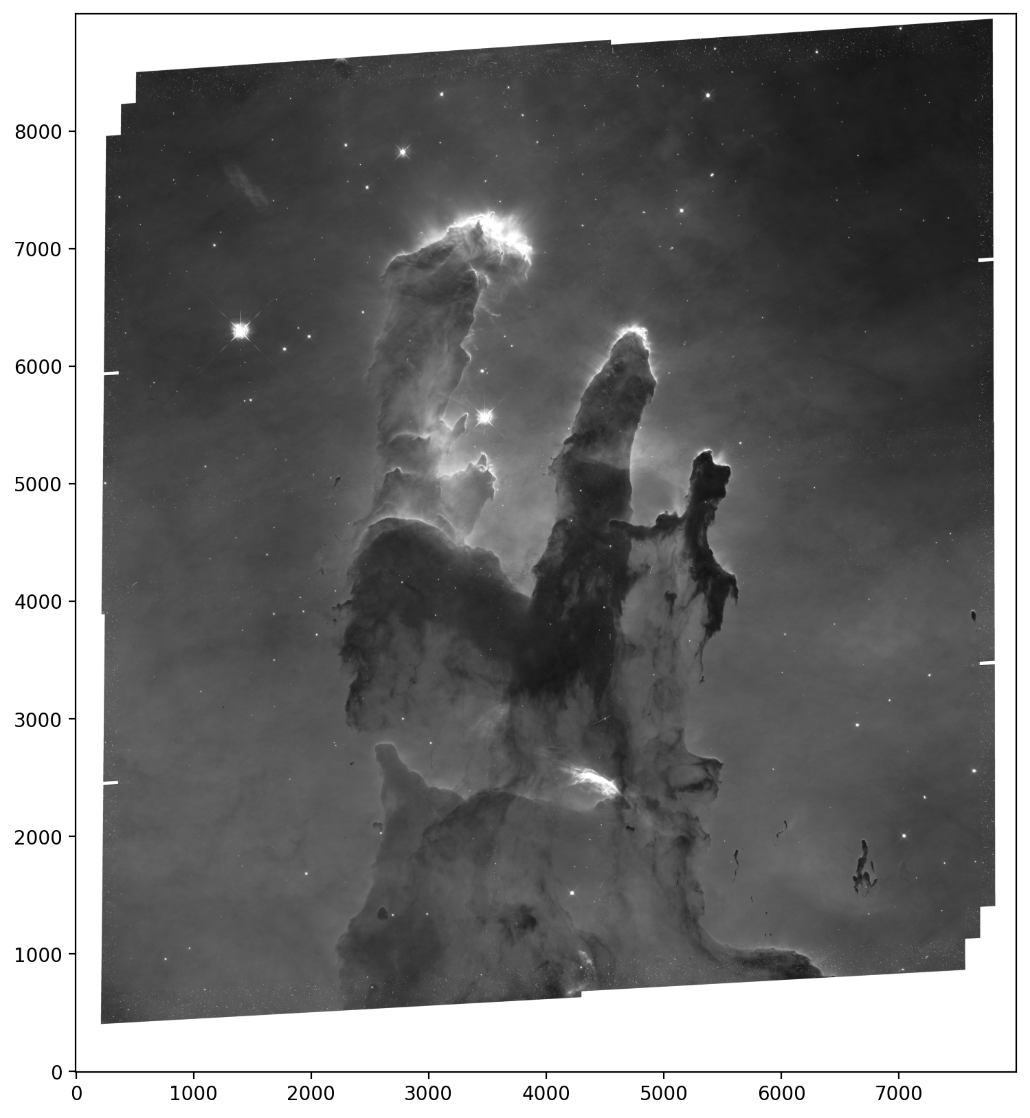
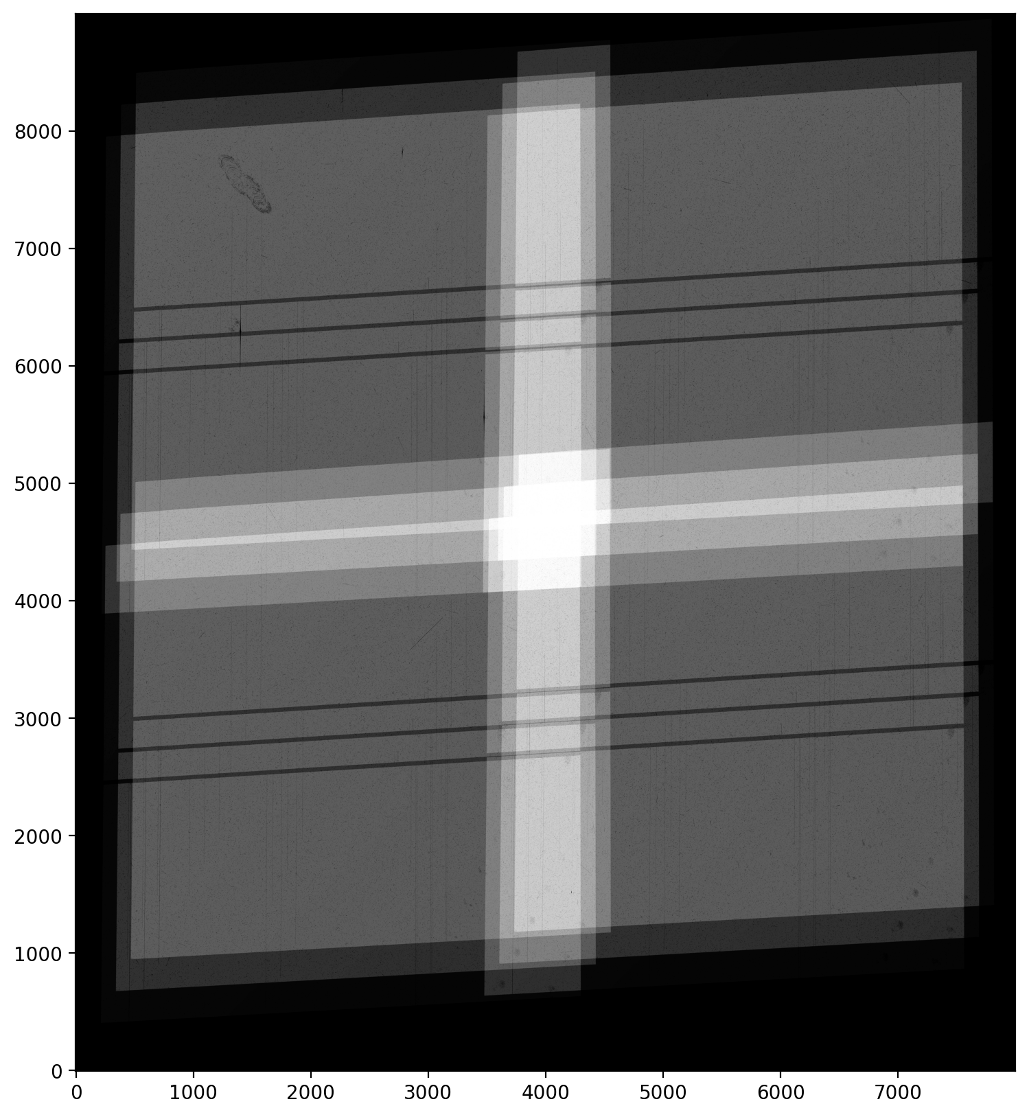
7.2 Display the combined DRZ science and weight images #
sci = fits.getdata('f160w_drz_sci.fits')
fig = plt.figure(figsize=(10, 10), dpi=140)
z1, z2 = zscale.get_limits(sci)
plt.imshow(sci, vmin=z1, vmax=z2, cmap='Greys_r', origin='lower')
plt.colorbar(shrink=0.8, pad=0.01)
<matplotlib.colorbar.Colorbar at 0x7efdd6579e50>
wht = fits.getdata('f160w_drz_wht.fits')
fig = plt.figure(figsize=(10, 10), dpi=140)
plt.imshow(wht, vmin=0, vmax=1700, cmap='Greys_r', origin='lower')
plt.colorbar(shrink=0.8, pad=0.01)
<matplotlib.colorbar.Colorbar at 0x7efdd66ea9d0>
8. Align the UVIS FLC frames to the IR mosaic #
The F160W drizzled mosaic defines the reference frame for aligning the UVIS filters. In ISR 2015-09, the UVIS visit-level DRC frames were aligned directly to the IR reference image, and this approach was chosen because the long UVIS exposures contain numerous cosmic-rays and relatively few point sources. The DrizzlePac task TweakBack was then used to propagate the updated WCS from the drizzled image header back to the individual FLC input frames making up each association prior to drizzling.
In this notebook, we instead align the UVIS FLC frames directly to the Gaia catalog, making use of a parameter in TweakReg which allows for specific flags in the DQ array of the FLC frames to be used or ignored. The imagefindpars parameter dqbits may be prepended with tilda to the string value to indicate which DQ flags to consider as “bad” pixels. For example, when deriving source catalogs, Tweakreg will ignore any pixels flagged as cosmic-ray flags in the MAST visit-level drizzled data products when dqbits is set to ~4096. This dramatically cuts down the number of false detections due to cosmic rays in the input FLC science arrays. More details on imagefindpars options may be found on the following webpage.
In this example, the threshold value was manually adjusted to get ~100 matches per UVIS exposure. Note that setting the threshold to a very low value does not necessarily translate to a better solution, since all sources are weighted equally when computing fits to match catalogs. This is especially relevant for UVIS data where CTE tails can shift the centroid position slightly along the readout direction for faint sources and potentially bias the fit.
refcat = 'gaia_pm.cat'   # Choose the Gaia catalog with proper motion data
cw = 3.5                 # Set to two times the FWHM of the PSF. (3.5 pixels for UVIS, 2.5 pixels for IR)
wcsname = 'UVIS_FLT'       # Specify the WCS name for this alignment

uvis_flcs = sorted(glob.glob('*flc.fits'))

tweakreg.TweakReg(uvis_flcs,
                  updatehdr=False,                                  # DO NOT UPDATE the header yet
                  refcat=refcat,
                  imagefindcfg={'threshold': 40., 'conv_width': cw, 'dqbits': "~4096"},
                  interactive=False, see2dplot=False,
                  shiftfile=True,
                  outshifts='shift657_flc.txt',
                  wcsname=wcsname,                                  # Give our WCS a unique name
                  reusename=True,
                  searchrad=0.3,
                  sigma=3,
                  ylimit=0.4,
                  fitgeometry='rscale')                             # Fit geometry (shift, rotation, scale)
clear_output()
# If the alignment is unsuccessful, stop the notebook

with open('shift657_flc.txt', 'r') as shift:
    for line_number, line in enumerate(shift, start=1):
        if "nan" in line:
            raise ValueError('nan found in line {} in shift file'.format(line_number))
        else:
            continue
8.1 Inspect the shift file to verify the pointing residuals #
Because each visit was acquired using a unique pair of Guide Stars, the three FLC exposures making up each visit should have roughly similar residual corrections to the WCS, which can be seen in the table below. Since the residuals in the shift file are close to zero and the rms values are <0.1 pixel, we can be confident that the fitting was successful.
shift_table = Table.read('shift657_flc.txt', format='ascii.no_header', names=['file', 'dx', 'dy', 'rot', 'scale', 'xrms', 'yrms'])

formats = ['.2f', '.2f', '.3f', '.5f', '.2f', '.2f']
for i, col in enumerate(shift_table.colnames[1:]):
    shift_table[col].format = formats[i]
shift_table
| file | dx | dy | rot | scale | xrms | yrms |
|---|---|---|---|---|---|---|
| str18 | float64 | float64 | float64 | float64 | float64 | float64 |
| ick905k5q_flc.fits | 0.01 | 0.07 | 360.000 | 0.99998 | 0.06 | 0.05 |
| ick905keq_flc.fits | -0.02 | 0.01 | 0.000 | 1.00000 | 0.05 | 0.04 |
| ick905knq_flc.fits | 0.03 | 0.01 | 359.999 | 0.99999 | 0.05 | 0.04 |
| ick906kwq_flc.fits | -0.01 | -0.02 | 0.000 | 1.00000 | 0.06 | 0.06 |
| ick906l5q_flc.fits | 0.01 | -0.01 | 360.000 | 1.00000 | 0.06 | 0.05 |
| ick906leq_flc.fits | -0.14 | 0.18 | 359.997 | 0.99999 | 0.05 | 0.05 |
| ick907nkq_flc.fits | -0.01 | 0.04 | 359.999 | 1.00000 | 0.06 | 0.04 |
| ick907o1q_flc.fits | 0.04 | 0.04 | 0.001 | 0.99999 | 0.05 | 0.04 |
| ick907ouq_flc.fits | 0.01 | 0.07 | 0.000 | 1.00001 | 0.05 | 0.05 |
| ick908pbq_flc.fits | 0.02 | 0.01 | 0.000 | 1.00001 | 0.03 | 0.03 |
| ick908pkq_flc.fits | 0.03 | 0.01 | 0.001 | 1.00001 | 0.04 | 0.04 |
| ick908ptq_flc.fits | 0.03 | 0.01 | 0.000 | 1.00000 | 0.04 | 0.04 |
# Print the Number of Gaia Matches per image from the TweakReg output
match_files = sorted(glob.glob('*_flc_catalog_fit.match'))
for f in match_files:
    input = ascii.read(f)
    print('Number of matches for', f, '= ', len(input))
Number of matches for ick905k5q_flc_catalog_fit.match =  137
Number of matches for ick905keq_flc_catalog_fit.match =  131
Number of matches for ick905knq_flc_catalog_fit.match =  119
Number of matches for ick906kwq_flc_catalog_fit.match =  142
Number of matches for ick906l5q_flc_catalog_fit.match =  136
Number of matches for ick906leq_flc_catalog_fit.match =  135
Number of matches for ick907nkq_flc_catalog_fit.match =  71
Number of matches for ick907o1q_flc_catalog_fit.match =  76
Number of matches for ick907ouq_flc_catalog_fit.match =  75
Number of matches for ick908pbq_flc_catalog_fit.match =  78
Number of matches for ick908pkq_flc_catalog_fit.match =  81
Number of matches for ick908ptq_flc_catalog_fit.match =  77
Compare the RMS and number of Matches from TweakReg with the MAST alignment results.
mast_uvis_wcs
| filename | DETECTOR | WCSNAME | NMATCHES | RMS_RA | RMS_DEC | RMS_RApix | RMS_DECpix |
|---|---|---|---|---|---|---|---|
| str18 | str4 | str30 | int64 | float64 | float64 | float64 | float64 |
| ick905k5q_flc.fits | UVIS | IDC_2731450pi-FIT_REL_GAIAeDR3 | 161 | 5.7 | 3.9 | 0.14 | 0.1 |
| ick905keq_flc.fits | UVIS | IDC_2731450pi-FIT_REL_GAIAeDR3 | 161 | 5.7 | 3.9 | 0.14 | 0.1 |
| ick905knq_flc.fits | UVIS | IDC_2731450pi-FIT_REL_GAIAeDR3 | 161 | 5.7 | 3.9 | 0.14 | 0.1 |
| ick906kwq_flc.fits | UVIS | IDC_2731450pi-FIT_IMG_GAIAeDR3 | 135 | 5.7 | 4.1 | 0.14 | 0.1 |
| ick906l5q_flc.fits | UVIS | IDC_2731450pi-FIT_IMG_GAIAeDR3 | 131 | 4.5 | 3.9 | 0.11 | 0.1 |
| ick906leq_flc.fits | UVIS | IDC_2731450pi-FIT_IMG_GAIAeDR3 | 72 | 15.9 | 15.6 | 0.4 | 0.39 |
| ick907nkq_flc.fits | UVIS | IDC_2731450pi-FIT_REL_GAIAeDR3 | 87 | 4.6 | 4.2 | 0.12 | 0.11 |
| ick907o1q_flc.fits | UVIS | IDC_2731450pi-FIT_REL_GAIAeDR3 | 87 | 4.6 | 4.2 | 0.12 | 0.11 |
| ick907ouq_flc.fits | UVIS | IDC_2731450pi-FIT_REL_GAIAeDR3 | 87 | 4.6 | 4.2 | 0.12 | 0.11 |
| ick908pbq_flc.fits | UVIS | IDC_2731450pi-FIT_REL_GAIAeDR3 | 100 | 3.8 | 3.8 | 0.1 | 0.1 |
| ick908pkq_flc.fits | UVIS | IDC_2731450pi-FIT_REL_GAIAeDR3 | 100 | 3.8 | 3.8 | 0.1 | 0.1 |
| ick908ptq_flc.fits | UVIS | IDC_2731450pi-FIT_REL_GAIAeDR3 | 100 | 3.8 | 3.8 | 0.1 | 0.1 |
Note that there are similar numbers of stars matched during MAST processing and in our custom alignment, with no significant shift rotation or scale resiuals in the shift file. To verify this, we inspect the quality of the fitting in the next section.
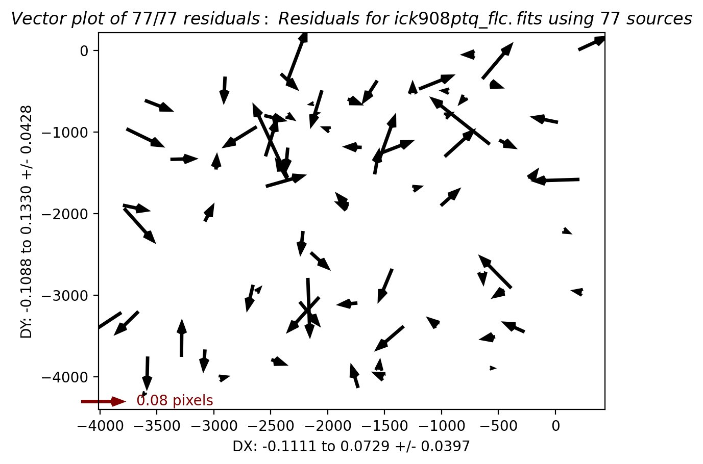
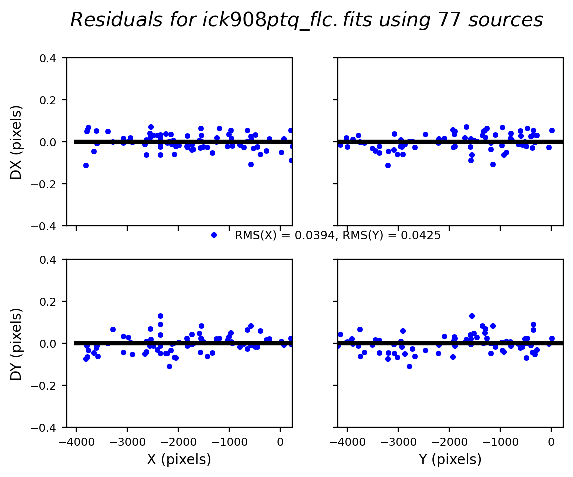
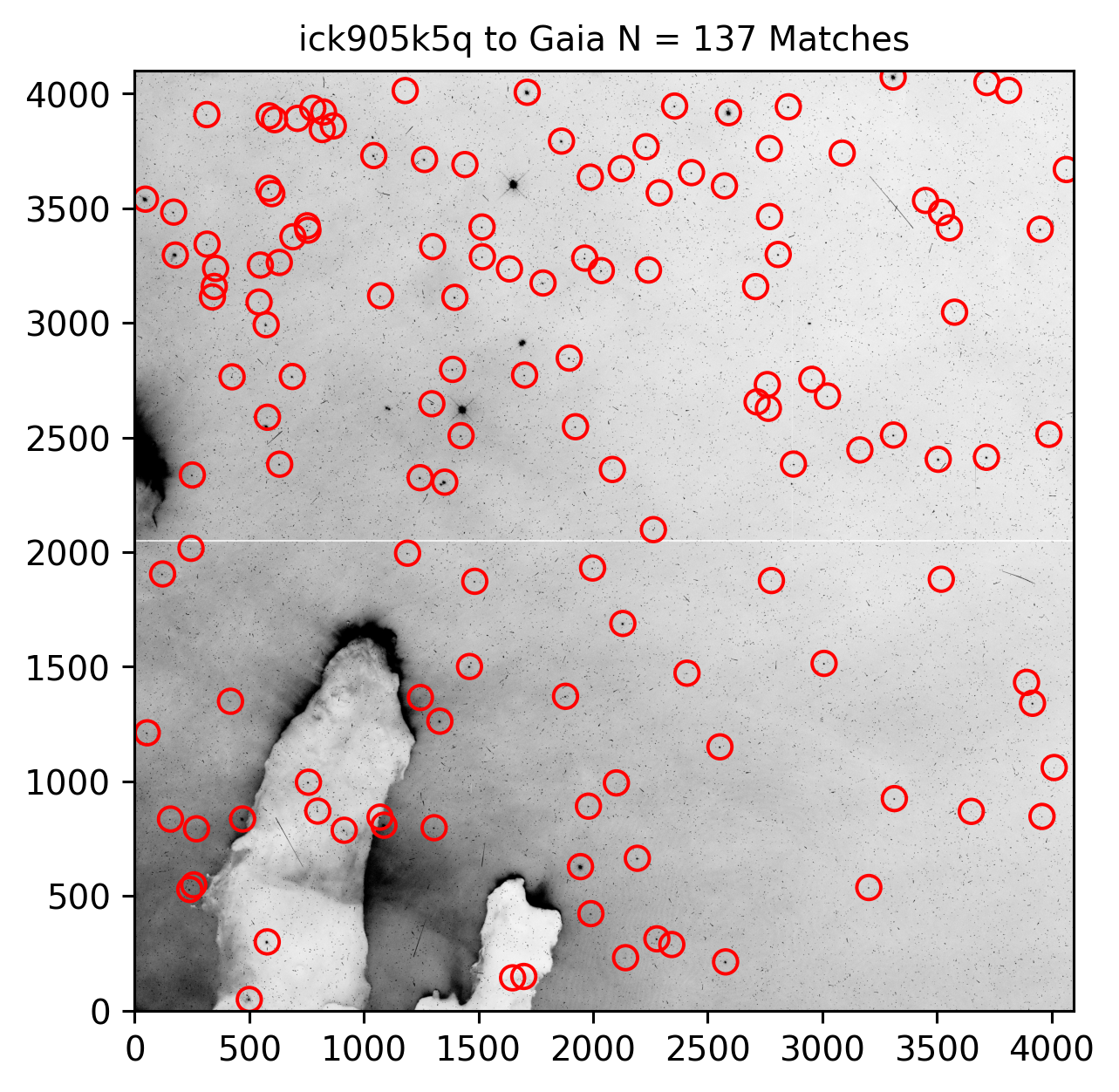
8.2 Inspect the UVIS fits #
Here, we overplot matched sources on the FLC frame, pasting the two chips together. In this example, we show only the first exposure in Visit 05, but additional visits may be inspected by uncommenting the lines below starting with rootname=.
rootname = 'ick905k5q'     # Visit 05a
# rootname = 'ick906kwq'   # Visit 06a
# rootname = 'ick907nkq'   # Visit 07a
# rootname = 'ick908pbq'   # Visit 08a

plt.figure(figsize=(5, 5), dpi=140)
chip1_data = fits.open(rootname+'_flc.fits')['SCI', 2].data
chip2_data = fits.open(rootname+'_flc.fits')['SCI', 1].data
fullsci = np.concatenate([chip2_data, chip1_data])
z1, z2 = zscale.get_limits(fullsci)
plt.imshow(fullsci, cmap='Greys', origin='lower', vmin=z1, vmax=z2)

match_tab = ascii.read(rootname+'_flc_catalog_fit.match')  # load match file in astropy table
match_tab_chip1 = match_tab[match_tab['col15'] == 2]   # filter table for sources on chip 1 (on ext 4)
match_tab_chip2 = match_tab[match_tab['col15'] == 1]   # filter table for sources on chip 2 (on ext 1)
x_cord1, y_cord1 = match_tab_chip1['col11'], match_tab_chip1['col12']
x_cord2, y_cord2 = match_tab_chip2['col11'], match_tab_chip2['col12']

plt.scatter(x_cord1, y_cord1+2051, s=50, edgecolor='r', facecolor='None', label='Matched Sources')
plt.scatter(x_cord2, y_cord2, s=50, edgecolor='r', facecolor='None')
plt.title(f'{rootname} to Gaia N = {len(match_tab)} Matches', fontsize=10)
Text(0.5, 1.0, 'ick905k5q to Gaia N = 137 Matches')
# inspect residual PNG
Image(filename=f'residuals_{rootname}_flc.png', width=500, height=300)
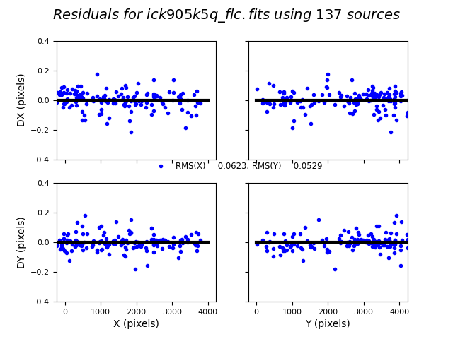
Below is the TweakReg call to update the header WCS. However since the shift file shows that the MAST alignment is good, we will not need to run this cell.
# tweakreg.TweakReg(uvis_flcs,
#                   updatehdr=True,                                  # Update the header
#                   refcat=refcat,
#                   interactive=False, see2dplot=False, shiftfile=False,
#                   imagefindcfg={'threshold':40.,'conv_width':cw,'dqbits': "~4096"},
#                   wcsname=wcsname,                                  # Give our WCS a unique name
#                   reusename=True,
#                   searchrad=0.3,
#                   sigma=3,
#                   ylimit=0.4,
#                   fitgeometry='rscale')                             # Fit geometry (shift, rotation, scale)
#  clear_output()
9. Drizzling the F657N mosaic #
Now that we have confirmed the alignment of the 12 FLC frames, these may be drizzled to a mosaic exactly half the scale (0.04”/pixel) of the original IR mosaic (0.08”/pixel). The same output WCS paramters: final_rot,final_ra, and final_dec values are used, but the final_outnx and final_outny are now twice the size of the IR mosaic at 8000x9000 pixels.
To save time for this notebook, the visit-level cosmic-ray flags for the individual UVIS tiles are assumed to be adequate, Steps 3, 4, 5, 6 are turned off, and the parameter resetbits is set to ‘0’ to avoid wiping out the 4096 flags in the FLC data quality arrays.
To improve processing speed, the sky background levels have been provided in advance and fed to AstroDrizzle via the skyfile parameter which reads in the input text file align_mosaics_uvis_skyfile.txt. Users would typically set skymethod='match' to compute the sky background levels, and this populates the image header keyword MDRIZSKY with the sky values in the imheader header of the FLC FITS files.
To further improve cosmic-ray rejection in the chip gap, AstroDrizzle may alternatively be run with all steps turned on as shown in the text below and with resetbits=4096 to update the DQ flags.
astrodrizzle.AstroDrizzle(input_uvis_images,
                          preserve=False, clean=False, build=False, context=False,
                          output='f657n_improved',
                          resetbits=4096,                              # Wipe out the CR flags
                          skymethod='match',                           # Sky Matching takes a lot of memory
                          combine_type='minmed',
                          final_bits='64,16',
                          final_wcs=True, final_scale=0.04, final_rot=-35,
                          final_ra=274.721587,final_dec=-13.841549,
                          final_outnx=8000, final_outny=9000)
input_uvis_images = sorted(glob.glob('*flc.fits'))

adriz(input_uvis_images,
      preserve=False, clean=False, build=False, context=False,
      output='f657n',
      driz_separate=False, median=False, blot=False, driz_cr=False,   # Turn off CR rejection steps
      resetbits=0,                                                    # Do not wipe out the MAST DQ flags
      skyfile='align_mosaics_uvis_skyfile.txt',                       # Provide user-defined sky values
      final_bits='64, 16',
      final_wcs=True, final_scale=0.04, final_rot=-35,                # Set the output WCS
      final_ra=274.721587, final_dec=-13.841549,
      final_outnx=8000, final_outny=9000)

clear_output()
9.1 Display the combined DRC science and weight images #
sci = fits.getdata('f657n_drc_sci.fits')
fig = plt.figure(figsize=(10, 10))
plt.imshow(sci, vmin=0, vmax=1, cmap='Greys_r', origin='lower')
<matplotlib.image.AxesImage at 0x7efdd461d910>
sci = fits.getdata('f657n_drc_wht.fits')
fig = plt.figure(figsize=(10, 10))
plt.imshow(sci, vmin=500, vmax=5000, cmap='Greys_r', origin='lower')
<matplotlib.image.AxesImage at 0x7efdd6c15490>
10. Conclusions #
This notebook provides the methodology for creating UVIS and IR mosaics of M16, as well as recommendations for key parameters. As such, it is relevant for users combining multi-visit observations from any HST imaging program, whether mosaics or single pointings.
For more detail on aligning to an absolute reference catalog such as GAIA, see the notebook ‘aligning_to_catalogs.ipynb’.
Thank you for walking through this notebook. You should be more familiar with:
Downloading data with astroquery.
Examining the active WCS.
Creating a reference catalog and aligning a dataset to it.
Checking tweakreg results.
Drizzling two detectors to the same output
Congratulations, you have completed the notebook.
Additional Resources #
Try to weave resource links into the main content of your tutorial so that they are falling in line with the context of your writing. For resources that do not fit cleanly into your narrative, you may include an additional resources section at the end of your tutorial. Usually a list of links using markdown bullet list plus link format is appropriate.
Below are some additional resources that may be helpful. Please send any questions through the HST Help Desk.
-
See Section 3.4.1 for documentation on
wf3cte, WFC3’s CTE correction pipelineSee Section 6 for documentation on WFC3/UVIS CTE
About this Notebook #
Created: 14 Dec 2018;     J. Mack
Updated: 02 Aug 2024;     J. Mack & B. Kuhn
Source: GitHub spacetelescope/hst_notebooks
Citations #
Provide your reader with guidelines on how to cite open source software and other resources in their own published work.
If you use Python packages such as astropy, astroquery, drizzlepac, matplotlib, or numpy for published research, please cite the
authors. Follow these links for more information about citing various packages.
