
Slitlessutils Cookbook: Spectral Extraction for ACS/WFC Subarrays#
This notebook contains a step-by-step guide for performing spectral extractions with Slitlessutils for G800L subarray data from ACS/WFC.
The original source for this notebook is the ACS folder on the spacetelescope/hst_notebooks GitHub repository.
Learning Goals#
In this tutorial you will:
Configure
SlitlessutilsDownload data
Preprocess data for extraction
Embed subarray images
Extract 1-D spectra with a simple boxcar method
Table of Contents#
1. Introduction
1.1 Environment
1.2 Imports
1.3 Slitlessutils Configuration
2. Define Global Variables
3. Download Data
3.1 Create Data Directories and Organize
4. Check the WCS
5. Preprocess the G800L Grism Images
6. Embed Subarray Data
7. Preprocess the F775W Direct Images
7.1 Display Drizzle Image and Overlay Segmentation Map
8. Extract the Spectra from the Grism Data
8.1 Display a Region File
8.2 Plot the Spectrum
9. Conclusions
Additional Resources
About this Notebook
Citations
1. Introduction#
Slitlessutils is an official STScI-supported Python package that provides spectral extraction processes for HST grism and
prism data. The slitlessutils software package has formally replaced the HSTaXe Python package, which will remain
on the spacetelescope GitHub organization, but no longer be maintained or developed.
Below, we show an example workflow of spectral extraction using ACS/WFC G800L grism data and F775W direct image data.
The example data were taken as part of ACS CAL program 15401 and are downloaded from MAST via astroquery. The images
are all subarray exposures, which require special preprocessing steps, mainly embedding the data into a full chip image. There
is an embedding utility within slitlessutils that we will use before processing and extracting the data.
Running this notebook requires creating a conda environment from the provided requirements file in this notebook’s
sub-folder in the GitHub repository. For more details about creating the necessary environment see the next section. This
tutorial is intended to run continuously without requiring any edits to the cells.
To run slitlessutils, we must download the configuration reference files. These files are instrument-specific and include
sensitivity curves, trace and dispersion files, flat fields, and more. Slitlessutils has a Config class with an associated
function that will download the necessary reference files from a public Box folder. Section 1.3 shows how to use slitlessutils
to retrieve the files. Once downloaded, slitlessutils will use them for the different processes.
1.1 Environment#
This notebook requires users to install the packages listed in the requirements.txt file located in the notebook’s
sub-folder on the GitHub repository. We will use the conda package manager to build the necessary virtual environment.
For more information about installing and getting started with Conda (or Mamba) please see this page.
First, we will make sure the conda-forge channel is added so that conda can correctly find the various packages.
$ conda config --add channels conda-forge
Next, we will create a new environment called slitlessutils and initialize it with python:
$ conda create --name slitlessutils "python==3.12"
Wait for conda to solve for the environment and confirm the packages/libraries with the y key when prompted.
Once completed you can activate the new environment with:
$ conda activate slitlessutils
With the new environment activated, we can install the remaining packages from the requirements.txt file with pip:
$ pip install -r requirements.txt
Note, you may encounter an error installing llvmlite. To fix it, run the below command before installing slitlessutils:
$ conda install -c conda-forge llvmlite
We have now successfully installed all the necessary packages for running this notebook. Launch Jupyter and begin:
$ jupyter-lab
1.2 Imports#
For this notebook we import:
| Package | Purpose |
|---|---|
glob |
File handling |
matplotlib.pyplot |
Displaying images and plotting spectrum |
numpy |
Handling arrays |
os |
System commands |
shutil |
File and directory clean up |
astropy.io.fits |
Reading and modifying/creating FITS files |
astropy.visualization |
Various tools for display FITS images |
astropy.wcs.WCS |
Handling WCS objects |
astroquery.mast.Observations |
Downloading FLT data from MAST |
drizzlepac.astrodrizzle |
Creating a mosaic for the direct image filter |
pyregions |
Overlaying DS9-formatted regions |
slitlessutils |
Handling preprocessing and spectral extraction |
#%matplotlib widget
import glob
import matplotlib.pyplot as plt
import numpy as np
import os
import shutil

from astropy.io import fits
from astropy.visualization import ZScaleInterval, ImageNormalize, LogStretch
from astropy.wcs import WCS
from astroquery.mast import Observations
from drizzlepac import astrodrizzle
import pyregion

import slitlessutils as su

zscale = ZScaleInterval()
INFO MainProcess> Logger (slitlessutils) with level=10 at 2026-04-07 16:33:03.888111
1.3 Slitlessutils Configuration#
In order to extract or simulate grism spectra with slitlessutils you must have the necessary reference files.
Below, we provide a table of file descriptions, example filenames, and file types for the different reference files
required by slitlessutils.
| File Description | Example Filename | File Type |
|---|---|---|
| Sensitivity curves for the different spectral orders | ACS.WFC.G800L.+1.sens.fits |
FITS table |
| Config files with trace and dispersion coefficients | ACS.WFC.G800L.CHIP1.conf |
Text / ASCII |
| Instrument configuration parameters | hst_acswfc.yaml |
YAML |
| Normalized sky images | ACS_WFC_G800L_smooth_sky.fits |
FITS image |
| Filter throughput curves | hst_acs_f775w.fits |
FITS table |
These reference files that are required for spectral extraction and modeling with slitlessutils must reside in a
dot-directory within the user’s home directory, {$HOME}/.slitlessutils. Upon initialization, the Config()
object verifies the existence of this directory and the presence of valid reference files. If the directory does not
exist, it is created; if the reference files are missing, the most recent versions are automatically retrieved from a
public Box directory. Once the files are downloaded, slitlessutils will apply them automatically, relieving the
user from calling them manually. For more information about configuring slitlessutils, please see the
documentation here.
In the following code cell, we initialize the configuration with su.config.Config(). As stated above, if this is your
first time initializing slitlessutils configuration, su.config.Config() will download the most recent reference
files. In the future, if a new reference file version is released it can be retrieved with cfg.retrieve_reffiles(update=True).
# Initialize configuration
cfg = su.config.Config()

# Optional download of new versions of reference files
#cfg.retrieve_reffiles()
INFO MainProcess> Using reference path: /home/runner/.slitlessutils/1.0.8/
2. Define Global Variables#
These variables will be use throughout the notebook and should only be updated if you are processing different datasets.
RA and DEC should be the precise location of the source in the direct image. Header keywords RA_TARG and DEC_TARG
are not always the most precise coordinates for the active WCS.
Note, the AB mag zeropoint for the direct image filter (here, F775W) is needed for SourceCollection. It is used by slitlessutils
to measure the magnitude within the aperture, which allows users to reject sources that are too faint. The value used for zeropoint will not
affect the resulting spectrum. Zeropoints for ACS/WFC filters can be found via the calculator here.
# the observations
FILTER = 'F775W' # direct image filter
GRATING = 'G800L'  # grism image filter
INSTRUMENT = 'ACS'
TELESCOPE = 'HST'

# datasets to process
DATASETS = {GRATING: ["jdql01jjq"],
            FILTER: ["jdql01jiq"]}

# target location
RA = 264.1018133 # degrees
DEC = -32.9086067 # degrees

# segmap and drizzling inputs and outputs
RAD = 0.5 # arcsec; for seg map
SCALE = 0.05 # driz image pix scale
ROOT = 'ACS_WFC_WRAY-15-1736' # output rootname for driz and later SU

# AB mag zeropoint for F775W for MJD 58153
ZEROPOINT = 25.657
3. Download Data#
Here, we download the example images via astroquery. For more information, please look at the documentation for
Astroquery, Astroquery.mast, and CAOM Field Descriptions, which is used for the obstab variable below. Additionally,
you may download the data from MAST using either the HST MAST Search Engine or the more general MAST Portal.
We download G800L and F775W _flt.fits images of the Wolf-Rayet star, WRAY 15-1736, from CAL
program 15401
(PI Hathi). This Wolf-Rayet star is relatively nearby and has bright emission lines, making it an ideal target for calibrating
the ACS/WFC grism (see ACS ISR 2019-01 (Hathi et al.) and references therein). After downloading the images, we move them to a
sub-directory within the current working directory.
Note: ACS subarray data taken after Servicing Mission 4 (SM4, May 2009), including the FLT files downloaded in the cells
below, contain bias striping noise that is not removed by the calibration pipeline (CALACS). To correct this bias striping noise
and perform the remaining data reduction steps, including CTE correction for supported subarrays, acstools.acs_destripe_plus
must be run on the RAW images. There is a notebook, available here, that guides users through the steps to reduce RAW
subarray data with acstools.acs_destripe_plus. To determine if your data can be CTE-corrected with this tool,
see Table 7.6 in the ACS Instrument Handbook. If you choose to reduce your data following that notebook, place the resulting
FLT or FLC files in the current working directory and proceed with Step 3.1.
def download(datasets, telescope):
    """
    Function to download FLT files from MAST with astroquery.
    `datasets` contains ROOTNAMEs i.e. `ipppssoot`.

    Parameters
    ----------
    datasets : dict
        Dictionary of grism and direct rootnames
    telescope : str
        Used for MAST; e.g. HST

    Output
    -------
    flt FITS files in current working dir
        ipppssoot_flt.fits
    """
    # Get user inputted datasets create list of rootname
    obs_ids = tuple(d.lower() for k, v in datasets.items() for d in v)

    # Query for all images with iels01*
    all_obs_table = Observations.query_criteria(obs_id=obs_ids[0][:6]+'*', obs_collection=telescope)

    # Get all the products
    products_table = Observations.get_product_list(all_obs_table)

    # Filter product list for user inputted obs_ids under variable DATASETS
    products_table = products_table[np.isin(products_table['obs_id'], obs_ids)]

    # Download the FLT files
    kwargs = {'productSubGroupDescription': 'FLT',
              'extension': 'fits',
              'cache': False}
    download_table = Observations.download_products(products_table, **kwargs)

    # Move the files to the cwd
    for local in download_table['Local Path']:
        local = str(local)
        f = os.path.basename(local)
        if f.startswith(obs_ids):
            shutil.copy2(local, '.')
download(DATASETS, TELESCOPE)
Downloading URL https://mast.stsci.edu/api/v0.1/Download/file?uri=mast:HST/product/jdql01jiq_flt.fits to ./mastDownload/HST/jdql01jiq/jdql01jiq_flt.fits ...
[Done]
Downloading URL https://mast.stsci.edu/api/v0.1/Download/file?uri=mast:HST/product/jdql01jjq_flt.fits to ./mastDownload/HST/jdql01jjq/jdql01jjq_flt.fits ...
[Done]
3.1 Create Data Directories and Organize#
Below, we define the current working directory, cwd, and create directories, g800l/, f775w/, and output/, that will be used
throughout the notebook. After the directories are created we move the downloaded FLT files into them.
cwd = os.getcwd()
print(f'The current directory is: {cwd}')
The current directory is: /home/runner/work/hst_notebooks/hst_notebooks/notebooks/ACS/acs_grism_extraction_subarray
dirs = [GRATING.lower(), FILTER.lower(), 'output']
for dirr in dirs:
    if os.path.isdir(dirr):
        print(f'Removing {dirr}/')
        shutil.rmtree(dirr)
    print(f'Creating {dirr}/')
    os.mkdir(dirr)
Removing g800l/
Creating g800l/
Removing f775w/
Creating f775w/
Removing output/
Creating output/
for file in glob.glob('*.fits'):
    filt = fits.getval(file, 'filter1').lower()
    print(f"Moving {file} to {filt}/")
    shutil.move(file, filt)
Moving jdql01jjq_flt.fits to g800l/
Moving jdql01jiq_flt.fits to f775w/
4. Check the WCS#
It is likely that the WCS in the direct and grism images differ. In this section we will use slitlessutils to view the active WCS.
To address any disagreement in WCS solutions, users can call the upgrade_wcs or downgrade_wcs functions within slitlessutils.
Slitlessutils also has the capability to downgrade the WCS to one of the other less complex solutions. Regardless of upgrading or
downgrading, it is imperative that the grism and direct images are on the same astrometric reference
for proper spectral extraction.
More information about slitlessutils astrometry can be found here. For a more technical and detailed understanding of HST WCS
and improved absolute astrometry please see ACS ISR 2022-03 (Mack et al.). A general overview is also available on Outerspace.
su.core.preprocess.astrometry.list_wcs(f'{GRATING.lower()}/j*flt.fits')
su.core.preprocess.astrometry.list_wcs(f'{FILTER.lower()}/j*flt.fits')
 g800l/jdql01jjq_flt.fits                    G800L
+----------+--------------------------------+--------------------------------+
| WCSVERS  |                              1 |
+----------+--------------------------------+--------------------------------+
| WCSNAME  |           IDC_4bb1536mj-GSC240 |
| WCSNAMEA |                  IDC_4bb1536mj |
| WCSNAMEB |           IDC_4bb1536mj-GSC240 |
| WCSNAMEO |                           OPUS |
+----------+--------------------------------+--------------------------------+


 f775w/jdql01jiq_flt.fits                    F775W
+----------+--------------------------------+--------------------------------+
| WCSVERS  |                              1 |
+----------+--------------------------------+--------------------------------+
| WCSNAME  | IDC_4bb1536mj-FIT_IMG_GAIAeDR3 |
| WCSNAMEA |                  IDC_4bb1536mj |
| WCSNAMEB |         IDC_4bb1536mj-GSC240-1 |
| WCSNAMEO |                           OPUS |
+----------+--------------------------------+--------------------------------+
As shown above, the F775W active WCS (IDC_4bb1536mj-FIT_IMG_GAIAeDR3) is different than the G800L WCS
(IDC_4bb1536mj-GSC240). It is crucial that all files have the same WCS solution for successful spectral extration.
To fix the discrepancy, we will use slitlessutils to downgrade the WCS of all the images to use the solution called
IDC_4bb1536mj. For this tutorial we are not concernced with precise absolute astrometry. The key requirement is
that the images have a consistent reference, which preserves relative source position.
files = glob.glob(f'{FILTER.lower()}/j*flt.fits') + glob.glob(f'{GRATING.lower()}/j*flt.fits')
for img in files:
    su.core.preprocess.astrometry.downgrade_wcs(img, key='A', inplace=True)
INFO MainProcess> downgrading WCS in f775w/jdql01jiq_flt.fits to WCSNAMEA
INFO MainProcess> downgrading WCS in g800l/jdql01jjq_flt.fits to WCSNAMEA
Finally, we print the active WCS name one last time to verify the upgrade worked as intended.
wcsnames = []
files = sorted(glob.glob(f'{GRATING.lower()}/j*flt.fits')+glob.glob(f'{FILTER.lower()}/j*flt.fits'))
for f in files:
    wcsname = fits.getval(f, 'WCSNAME', ext=1)
    wcsnames.append(wcsname)
    print(f, wcsname)

if len(set(wcsnames)) == 1:
    print("\nSuccess!\n")
else:
    print("\nThere is still more than one active WCS\n")
f775w/jdql01jiq_flt.fits IDC_4bb1536mj
g800l/jdql01jjq_flt.fits IDC_4bb1536mj

Success!
5. Embed Subarray Data#
In order to perform spectral extraction on subarray data with slitlessutils, the images must be embedded first.
To embed the subarray data we use the built in utility, embedsub_full_chip, within slitlessutils. This function
works on WFC3 (UVIS/IR) and ACS (WFC) subarrays and saves the original files as ipppssoot_flt_original.fits.
The embedded files will have modified LTV*, NAXIS*, CRPIX*, and SUBARRAY header keywords. The embedding
utility saves the original values at the end of the HISTORY section in the primary header. The old (original) values are
not needed, but were added for convenience and bookkeeping.
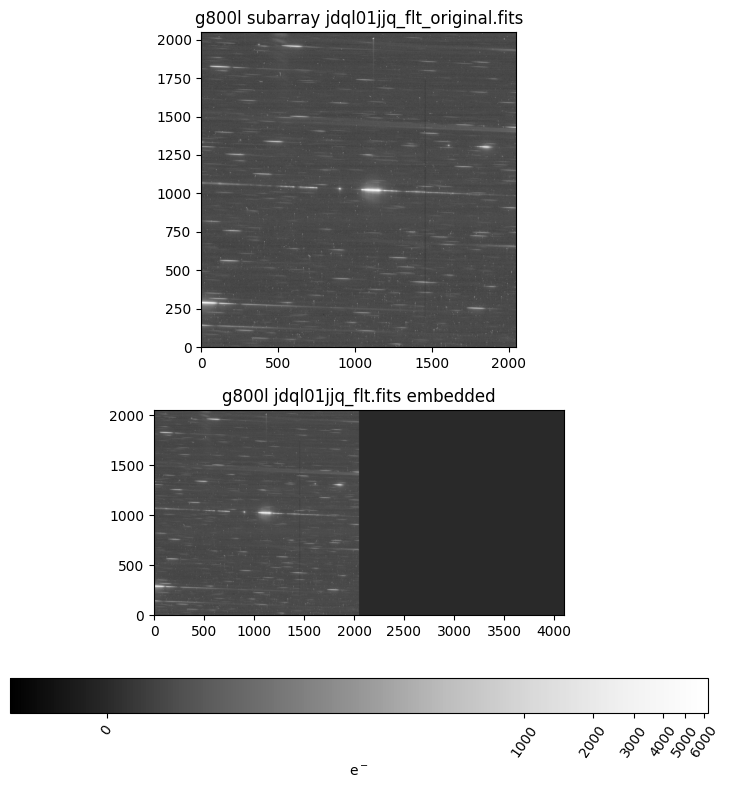
Below, we call the embedding function on the grism and direct images, and then create a subarray/ directory for
the original subarray files. Finally, we display an original an embedded grism image to verify it looks as expected.
We also show how the original header keywords are appended to the HISTORY section of an embedded file.
os.chdir(cwd)
# loop over all direct and grism images and embed subarray into full-chip image
for file in glob.glob(f"{FILTER.lower()}/*flt.fits")+glob.glob(f"{GRATING.lower()}/*flt.fits"):
    dirr = file.split('/')[0]
    su.core.utilities.embedding.embedsub_full_chip(file, instrument='WFC', output_dir=dirr)
# loop over all original direct and grism subarray images and move to new dir
for file in glob.glob(f"{FILTER.lower()}/*original.fits")+glob.glob(f"{GRATING.lower()}/*original.fits"):
    dirr = file.split('/')[0]
    dst = dirr+'/subarray'
    # create subarray directory
    if not os.path.isdir(dst):
        os.mkdir(dst)
    print(f"Moving {file} to {dst}/")
    shutil.move(f"{os.path.abspath('./')}/{file}",
                f"{os.path.abspath('./')}/{dst}/{file.split('/')[-1]}")
Moving f775w/jdql01jiq_flt_original.fits to f775w/subarray/
Moving g800l/jdql01jjq_flt_original.fits to g800l/subarray/
embed_file = f'{GRATING.lower()}/{DATASETS[GRATING][0]}_flt.fits'
orig_file = f'{GRATING.lower()}/subarray/{DATASETS[GRATING][0]}_flt_original.fits'

fig, [ax1, ax2] = plt.subplots(2, 1, figsize=(9, 9))
embed_img = fits.getdata(embed_file, ext=1)
orig_img = fits.getdata(orig_file, ext=1)

z1, z2 = zscale.get_limits(orig_img)
norm_embed = ImageNormalize(embed_img, vmin=z1, vmax=z2*100, stretch=LogStretch())
norm_orig = ImageNormalize(orig_img, vmin=z1, vmax=z2*100, stretch=LogStretch())

im1 = ax1.imshow(orig_img, origin='lower', cmap='Greys_r', norm=norm_orig)
im2 = ax2.imshow(embed_img, origin='lower', cmap='Greys_r', norm=norm_embed)
cbar2 = fig.colorbar(im2, ax=ax2, orientation='horizontal', pad=0.2, label='e$^-$')

ax1.set_title(f"{orig_file.replace('/', ' ')}")
ax2.set_title(f"{embed_file.replace('/', ' ')} embedded")
for t in cbar2.ax.get_xticklabels():
    t.set_rotation(55)
plt.show()
# the embedding function adds original keywords to HISTORY
fits.getval(embed_file, "HISTORY")[-5:]
This file was created with slitlessutils function, `embedsub_full_chip`
As a result, some header keywords have been modified:
    - CRPIX1 and CRPIX2 were originally: 2048.0, 1024.0
    - LTV1 and LTV2 were originally: 0.0, 0.0
    - NAXIS1 and NAXIS2 were originally: 2048, 2048
6. Preprocess the G800L Grism Images#
The function below performs preprocessing steps to prepare the grism images for optimal spectral extraction.
This function completes two tasks, (1) background subtraction via a master-sky image, and (2) cosmic ray
(CR) flagging via Laplacian edge detection.
In slitless spectroscopy, the background is inherently complex because every patch of sky is dispersed onto
the detector, and each spectral order has a different response and geometric footprint. This complexity is
further amplified by wavelength-dependent flat fields, resulting in a highly structured two-dimensional
background that cannot be treated like standard imaging backgrounds.
Slitlessutils handles this by subtracting a master-sky image, which is built from many science and
calibration exposures with sources removed, leaving only the instrumental and sky background structure.
This sky image is scaled to each individual exposure by fitting the sky-dominated pixels and is subtracted
before any further reduction steps. For more details about slitlessutils background subtraction see here.
Slitlessutils does not interpolate over CRs, and expects affected pixels to be flagged in the data quality
array. There are two methods in slitlessutils for identifying and flagging CRs: a Laplacian edge-detection
technique that identifies sharp, high-contrast features in individual images, and a drizzle-based approach that
uses AstroDrizzle to compare multiple aligned exposures and flag discrepant pixels. The Laplace method
works on single exposures using image gradients, while the drizzle method groups and aligns images before
identifying CRs from their inconsistencies.
Below, we flag CRs using the Laplacian edge detection method.
For more information about CR flagging
with slitlessutils see the documentation here.
def preprocess_grism(datasets, grating):
    """
    Function to perform bkg subtraction with master-sky image and CR flagging with drizzle

    Parameters
    ----------
    dataset : dict
        A dictionary of grating and filter rootnames
    grating : str
        The grism image filter associated with datasets; e.g. G800L
    """
    # Create a list of all G800L files
    grismfiles = [f'{grismdset}_flt.fits' for grismdset in datasets[grating]]

    # Subtract background via master-sky
    # Background subtraction should happen on original subarray images before embedding
    # Subtract sky before CR flagging
    back = su.core.preprocess.background.Background()
    for grism in grismfiles:
        back.image(grism, inplace=True)

    # Process FLTs through drizzle for CR flagging
    grismfiles = su.core.preprocess.crrej.laplace(grismfiles, inplace=True)
os.chdir(GRATING.lower())

preprocess_grism(DATASETS, GRATING)

os.chdir('..')
INFO MainProcess> Flagging cosmic rays with Laplacian kernel jdql01jjq_flt.fits
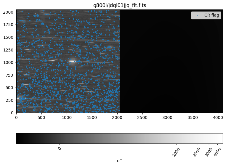
Next, we display one of the grism images and overlay the CR flags from the Data Qualty array for visual inspection.
fig, axs = plt.subplots(1, 1, figsize=(9, 9))

img = fits.getdata(f'{GRATING.lower()}/{DATASETS[GRATING][0]}_flt.fits', ext=1)
dq = fits.getdata(f'{GRATING.lower()}/{DATASETS[GRATING][0]}_flt.fits', ext=3)

z1, z2 = zscale.get_limits(img)
inorm = ImageNormalize(img, vmin=z1, vmax=z2*100, stretch=LogStretch())
im1 = axs.imshow(img, origin='lower', cmap='Greys_r', norm=inorm)
y, x = np.where(np.bitwise_and(dq, 4096) == 4096)
axs.scatter(x, y, 3, marker='.', label='CR flag')

axs.set_title(f'{GRATING.lower()}/{DATASETS[GRATING][0]}_flt.fits')
cbar = fig.colorbar(im1, ax=axs, orientation='horizontal', pad=0.1, label='e$^-$')
# plt.xlim(3000, 4000)
plt.legend()
for t in cbar.ax.get_xticklabels():
    t.set_rotation(55)
plt.show()
7. Preprocess the F775W Direct Image#
With the grism data calibrated, data embedded, and consistent WCS for all images, we can continue to the preprocessing of the
direct image. The two main steps we need to complete are (1) drizzling the direct image and (2) creating a segmentation map.
Information about drizzlepac can be found here, and astrodrizzle
tutorials are hosted in the hst_notebook GitHub repo.
def preprocess_direct(datasets, filt, root, scale, ra, dec, rad, telescope, instrument):
    """
    Function to create drizzle image and segmentation map for direct image data.

    Parameters
    ----------
    datasets : dict
        A dictionary of grating and filter rootnames
    filt : str
        The direct image filter associated with datasets
    root : str
        The filename for the drizzle image and seg. map
    scale : float
        Pixel (plate) scale for drizzle image and seg. map (arcsec)
    ra : float
        The Right Ascension of the source in the direct image (degrees)
    dec : float
        The Declination of the source in the direct image (degrees)
    rad : float
        The radius of the segmentation size (arcsec)
    telescope : str
        The name of the observatory; e.g. HST
    instrument : str
        The name of the instrument; e.g. WFC3

    Outputs
    -------
    Drizzle image : FITS file
        <root>_drz_sci.fits
    Segmentation map : FITS file
        <root>_drz_seg.fits
    """

    # list of direct image data
    files = [f'{imgdset}_flt.fits' for imgdset in datasets[filt]]

    # mosaic data via astrodrizzle
    astrodrizzle.AstroDrizzle(files, output=root, build=False,
                              static=False, skysub=False, driz_separate=False,
                              median=False, blot=False, driz_cr=False,
                              driz_combine=True, final_wcs=True,
                              final_rot=0., final_scale=scale,
                              final_pixfrac=1.0,
                              overwrite=True, final_fillval=0.0)

    # Must use memmap=False to force close all handles and allow file overwrite
    with fits.open(f'{root}_drz_sci.fits', memmap=False) as hdulist:
        img = hdulist['PRIMARY'].data
        hdr = hdulist['PRIMARY'].header

    wcs = WCS(hdr)
    x, y = wcs.all_world2pix(ra, dec, 0)

    xx, yy = np.meshgrid(np.arange(hdr['NAXIS1']),
                         np.arange(hdr['NAXIS2']))
    rr = np.hypot(xx-x, yy-y)
    seg = rr < (rad/scale)

    # add some keywords for SU
    hdr['TELESCOP'] = telescope
    hdr['INSTRUME'] = instrument
    hdr['FILTER'] = filt

    # write the files to disk
    fits.writeto(f'{root}_drz_sci.fits', img, hdr, overwrite=True)
    fits.writeto(f'{root}_drz_seg.fits', seg.astype(int), hdr, overwrite=True)
os.chdir(FILTER.lower())

preprocess_direct(DATASETS, FILTER, ROOT, SCALE, RA, DEC, RAD, TELESCOPE, INSTRUMENT)

os.chdir('..')
Setting up logfile : astrodrizzle.log
AstroDrizzle log file: astrodrizzle.log
AstroDrizzle Version 3.10.0 started at: 16:33:39.935 (07/04/2026)
==== Processing Step Initialization started at 16:33:39.937 (07/04/2026)
Forcibly archiving original of: jdql01jiq_flt.fits as OrIg_files/jdql01jiq_flt.fits
Turning OFF "preserve" and "restore" actions...
WCS Keywords
Number of WCS axes: 2
CTYPE : 'RA---TAN' 'DEC--TAN'
CUNIT : 'deg' 'deg'
CRVAL : 264.10285393154345 -32.92277572251619
CRPIX : 1274.5021349018505 2152.461136322904
CD1_1 CD1_2 : -1.388888888888889e-05 1.4671173289358916e-22
CD2_1 CD2_2 : 1.4112335586120426e-22 1.388888888888889e-05
NAXIS : 2549 4303
********************************************************************************
*
* Estimated memory usage: up to 189 Mb.
* Output image size: 2549 X 4303 pixels.
* Output image file: ~ 125 Mb.
* Cores available: 1
*
********************************************************************************
==== Processing Step Initialization finished at 16:33:40.248 (07/04/2026)
==== Processing Step Static Mask started at 16:33:40.250 (07/04/2026)
==== Processing Step Static Mask finished at 16:33:40.251 (07/04/2026)
==== Processing Step Subtract Sky started at 16:33:40.252 (07/04/2026)
==== Processing Step Subtract Sky finished at 16:33:40.280 (07/04/2026)
==== Processing Step Separate Drizzle started at 16:33:40.281 (07/04/2026)
==== Processing Step Separate Drizzle finished at 16:33:40.28 (07/04/2026)
==== Processing Step Create Median started at 16:33:40.283 (07/04/2026)
==== Processing Step Blot started at 16:33:40.285 (07/04/2026)
==== Processing Step Blot finished at 16:33:40.286 (07/04/2026)
==== Processing Step Driz_CR started at 16:33:40.286 (07/04/2026)
==== Processing Step Final Drizzle started at 16:33:40.2 (07/04/2026)
WCS Keywords
Number of WCS axes: 2
CTYPE : 'RA---TAN' 'DEC--TAN'
CUNIT : 'deg' 'deg'
CRVAL : 264.10285393154345 -32.92277572251619
CRPIX : 1274.5021349018505 2152.461136322904
CD1_1 CD1_2 : -1.388888888888889e-05 1.4671173289358916e-22
CD2_1 CD2_2 : 1.4112335586120426e-22 1.388888888888889e-05
NAXIS : 2549 4303
-Generating simple FITS output: ACS_WFC_WRAY-15-1736_drz_sci.fits
Writing out image to disk: ACS_WFC_WRAY-15-1736_drz_sci.fits
Writing out image to disk: ACS_WFC_WRAY-15-1736_drz_wht.fits
Writing out image to disk: ACS_WFC_WRAY-15-1736_drz_ctx.fits
==== Processing Step Final Drizzle finished at 16:33:42.42 (07/04/2026)
AstroDrizzle Version 3.10.0 is finished processing at 16:33:42.425 (07/04/2026).
-------------------- --------------------
Step Elapsed time
-------------------- --------------------
Initialization 0.3115 sec.
Static Mask 0.0016 sec.
Subtract Sky 0.0279 sec.
Separate Drizzle 0.0016 sec.
Create Median 0.0000 sec.
Blot 0.0011 sec.
Driz_CR 0.0000 sec.
Final Drizzle 2.1352 sec.
==================== ====================
Total 2.4788 sec.
Trailer file written to: astrodrizzle.log
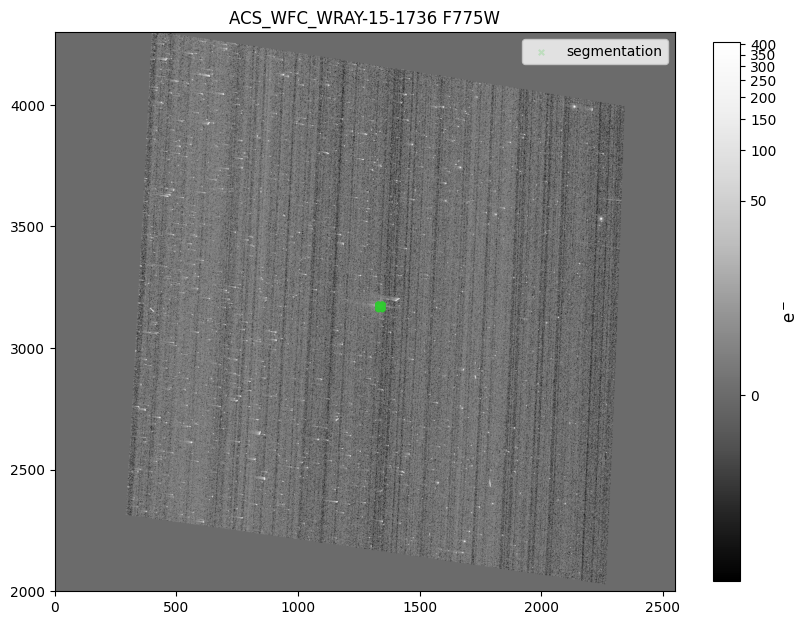
7.1 Display Drizzle Image and Overlay Segmentation Map#
Next, we display the F775W drizzle image created in the cell above. We also overplot the segmentation map by getting all
the x and y pixels where the segmentation array is True. Visually inspect the drizzle science image (and other drizzle
products if needed) for accurate image alignment and combination, as well as the source location as defined by the
segmentation map.
# get drizzle data
d = fits.getdata(f'{FILTER.lower()}/{ROOT}_drz_sci.fits')
# get seg map coordinates
y, x = np.where(fits.getdata(f'{FILTER.lower()}/{ROOT}_drz_seg.fits') == 1)

# display the image and seg map coords
fig, axs = plt.subplots(1, 1, figsize=(10, 10))
z1, z2 = zscale.get_limits(d)
inorm = ImageNormalize(d, vmin=z1, vmax=z2*100, stretch=LogStretch())
im1 = axs.imshow(d, origin='lower', cmap='Greys_r', norm=inorm)
axs.scatter(x, y, 15, marker='x', c='limegreen', alpha=0.2, label='segmentation')
fig.colorbar(im1, ax=axs, shrink=0.7).set_label(label='e$^-$', size=12)
axs.set_ylim(2000,4300)
axs.set_title(f'{ROOT} {FILTER}')
axs.legend()
plt.show()
8. Extract the Spectrum from the Grism Data#
We are now finished with all the preprocessing steps and ready to extract the 1D spectrum. The function below demonstrates a complete
single-orientation spectral extraction workflow using slitlessutils, starting from calibrated ACS/WFC grism exposures and a direct-image–
based source catalog (segmentation map).
First, the files are loaded into WFSSCollection, which serves as a container for the grism FLT exposures used in the extraction. Grouping
them into a collection allows slitlessutils to treat the set of exposures as a unified dataset when projecting sources, building pixel‑dispersion
tables (PDTs), and performing extraction. For more information about WFSSCollection see the documentation here.
Next, sources are defined using the segmentation map and drizzled science image from the associated direct filter, which are initialized into a
SourceCollection data structure. For more information about SourceCollection see the documentation here.
The Region module creates visual outlines of where each source’s dispersed light appears on the grism images. It does this by reading
the PDTs and distilling them into DS9‑compatible region files that trace the footprint of each spectral order across the detector. These
region files are not required for extraction, but are useful for quickly inspecting which parts of the grism images contribute to each object’s
spectrum. More information about Region can be found here.
Tabulate performs the forward‑modeling step that connects the direct image to the grism frames. For every relevant direct‑image pixel,
it computes the trace, wavelength mapping, and fractional pixel coverage and stores the results in a PDT. Because this calculation is
computationally expensive, slitlessutils only computes PDTs when requested and then saves them in hierarchical data-format 5 (HDF5)
files inside the su_tables/ directory for later use. The PDT files only capture the geometric mapping of the scene. Instrumental effects and
the actual astrophysical signal are added later in the workflow, so the PDTs depend solely on the WCS and its calibration. See the Tabulate
documentation for more information.
Finally, the Single class carries out the one‑dimensional extraction for a single telescope orientation (position angle) and spectral
order (here, the +1 order). It uses the PDTs to forward‑model how each direct‑image pixel contributes to the dispersed spectrum and
assembles these contributions into a 1D spectrum. The method is conceptually similar to HSTaXe, but with a more flexible contamination
model and a full forward‑modeling approach that can support optimization such as SED‑fitting workflows. This extraction mode is intended
for relatively simple, isolated sources where self‑contamination is not severe. A given spectral order should be extracted one at a time. Note,
the software will overwrite the x1d.fits file so users must use unique file names with root. The documentation for Single can be
found here.
def extract_single(grating, filt, root, zeropoint, tabulate=False):
    """
    Basic single orient extraction similar to HSTaXe

    Parameters
    ----------
    grating : str
        The grism image filter associated with datasets; e.g. G280
    filt : str
        The direct image filter associated with datasets e.g. F200LP
    root : str
        The rootname of the drz and seg FITS file; will also be the 1d spectrum output file rootname
    zeropoint : float
        The AB mag zeropoint of the direct image filter; needed when simulating or rejecting faint sources
    tabulate : Bool
        If true, SU computes the pixel‑dispersion tables. Only need once per `data` and `sources`

    Output
    ------
    1D spectrum : FITS file
        root_x1d.fits

    """
    # load grism data into slitlessutils
    data = su.wfss.WFSSCollection.from_glob(f'../{grating.lower()}/*_flt.fits')

    # load the sources from direct image into slitlessutils
    sources = su.sources.SourceCollection(f'../{filt.lower()}/{root}_drz_seg.fits',
                                          f'../{filt.lower()}/{root}_drz_sci.fits',
                                          local_back=False,
                                          zeropoint=zeropoint)

    # create region files for spectral orders
    # regions are NOT required for spectral extraction
    reg = su.modules.Region(ncpu=1, orders=['+1', '+2', '-1', '-2'])
    reg(data, sources)

    # project the sources onto the grism images; output to `su_tables/`
    if tabulate:
        tab = su.modules.Tabulate(ncpu=1)
        tab(data, sources)

    # run a single-orient extraction on the +1 order
    ext = su.modules.Single('+1', mskorders=None, root=root, ncpu=1)
    ext(data, sources, width=15)
os.chdir('output')

extract_single(GRATING, FILTER, ROOT, ZEROPOINT, tabulate=True)

os.chdir('..')
INFO MainProcess> Loading from glob: ../g800l/*_flt.fits
INFO MainProcess> Loading WFSS data from python list
INFO MainProcess> loading throughput from keys: ('hst', 'acs', 'f775w')
INFO MainProcess> Loading a classic segmentation map: ../f775w/ACS_WFC_WRAY-15-1736_drz_seg.fits
INFO MainProcess> Serial processing
Regions: 0%| | 0/1 [00:00<?, ?it/s]
Regions: 100%|██████████| 1/1 [00:00<00:00, 1.00it/s]
Regions: 100%|██████████| 1/1 [00:00<00:00, 1.00it/s]
INFO MainProcess> Serial processing
Tabulating: 0%| | 0/1 [00:00<?, ?it/s]
Tabulating: 100%|██████████| 1/1 [00:12<00:00, 12.65s/it]
Tabulating: 100%|██████████| 1/1 [00:12<00:00, 12.65s/it]
INFO MainProcess> Serial processing
Extracting (single): 0%| | 0/1 [00:00<?, ?it/s]
INFO MainProcess> Building contamination model for jdql01jjq/WFC2
Extracting (single): 100%|██████████| 1/1 [00:01<00:00, 1.18s/it]
Extracting (single): 100%|██████████| 1/1 [00:01<00:00, 1.18s/it]
INFO MainProcess> Combining the 1d spectra
INFO MainProcess> Writing: /home/runner/work/hst_notebooks/hst_notebooks/notebooks/ACS/acs_grism_extraction_subarray/output/ACS_WFC_WRAY-15-1736_x1d.fits
WARNING: VerifyWarning: Card is too long, comment will be truncated. [astropy.io.fits.card]
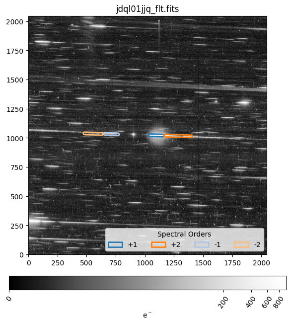
8.1 Display a Region File#
Below, we display a grism FLT file and the associated region file. The region files are useful for quickly inspecting which part
of the grism image contribute to each object’s spectrum. The +1, +2, -1, and -2 spectral orders for the observation are outlined in
dark blue, dark orange, light blue, and light orange respectively. More information about the slitlessutils region files can be
found here.
i = 0 # which FLT image to display
fig, axs = plt.subplots(1, 1, figsize=[8, 8])

region = pyregion.open(f'output/{DATASETS[GRATING][i]}_WFC2.reg')
patch_list, _ = region.get_mpl_patches_texts()
orders = ['+1', '+2', '-1', '-2']
for idx, p in enumerate(patch_list):
    p.set_linewidth(2)
    p.set_label(orders[idx])
    axs.add_patch(p)
axs.legend(title="Spectral Orders", ncol=4, loc='lower right')
axs.set_xlim(0,2048)

flt = fits.getdata(f'{GRATING.lower()}/{DATASETS[GRATING][i]}_flt.fits')
z1, z2 = zscale.get_limits(flt)
inorm = ImageNormalize(flt, vmin=0, vmax=z2*20, stretch=LogStretch())
im1 = axs.imshow(flt, origin='lower', cmap='Greys_r', norm=inorm)
axs.set_title(f'{DATASETS[GRATING][i]}_flt.fits')
cbar = fig.colorbar(im1, ax=axs, shrink=0.9, pad=0.07, orientation='horizontal', label='e$^-$')
for t in cbar.ax.get_xticklabels():
    t.set_rotation(55)

plt.show()
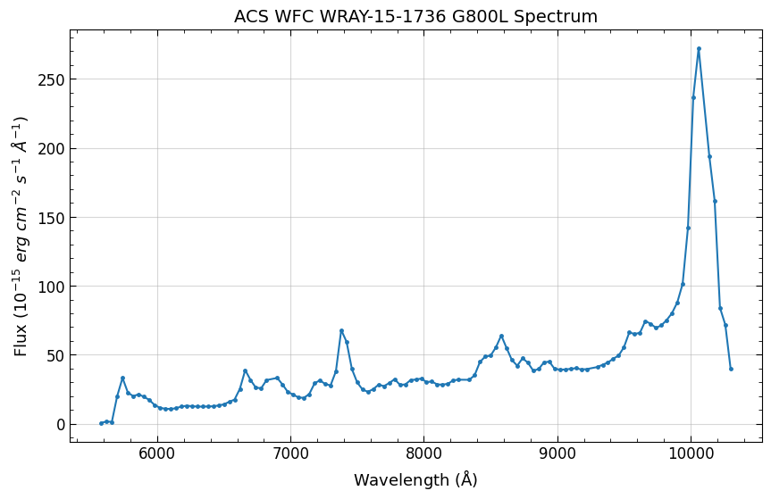
8.2 Plot the Spectrum#
Finally, what we’ve all been waiting for(!), plotting the extracted spectrum. The Single module produces a single spectrum for each
source and grism image. Those spectra are then combined together into a single one-dimensional spectrum for each source and saved
as a x1d.fits file. In this example, we only have one source so there is a single spectrum.
The x1d file is a binary table with columns for the wavelength (lamb), flux (flam), uncertainty (func), contamination (cont),
and number of pixels (npix). By default configuration, the flux and uncertainty values are in units of erg s-1 cm-2 · Å-1 and scaled by
10-17 (cfg.fluxunits and cfg.fluxscale)
cfg.fluxunits, cfg.fluxscale
('erg / (s * cm**2 * Angstrom)', 1e-17)
fig, ax = plt.subplots(1, 1, figsize=(10, 6))
ax.grid(alpha=0.5)

dat = fits.getdata(f'output/{ROOT}_x1d.fits')
lrange = (5000, 11000)
wav = np.where((lrange[0] < dat['wavelength']) & (dat['wavelength'] < lrange[1]))

ax.errorbar(dat['wavelength'][wav],
            dat['flux'][wav]*cfg.fluxscale/1e-15,
            yerr=dat['uncertainty'][wav]*cfg.fluxscale/1e-15,
            marker='.', markersize=5)

ax.minorticks_on()
ax.yaxis.set_ticks_position('both'), ax.xaxis.set_ticks_position('both')
ax.tick_params(axis='both', which='minor', direction='in', labelsize=12, length=3)
ax.tick_params(axis='both', which='major', direction='in', labelsize=12, length=5)
ax.set_xlabel(r'Wavelength ($\mathrm{\AA}$)', size=13)
ax.set_ylabel(r'Flux (10$^{-15}$ $erg\ cm^{-2}\ s^{-1}\ \AA^{-1}$)', size=13)
ax.set_title(f"{ROOT.replace('_', ' ')} {GRATING} Spectrum", size=14)
plt.show()
9. Conclusions#
Thank you for going through this notebook. You should now have all the necessary tools for extracting a
1D spectrum from WFC3 IR grism data with slitlessutils. After completing this notebook you should be more familiar with:
Downloading data.
Preprocessing images for slitlessutils.
Embedding subarray images
Creating and displaying region files.
Extracting and plotting a source’s spectrum
Additional Resources#
Below are some additional resources that may be helpful. Please send any questions through the HST Help Desk.
About this Notebook#
Author: Roberto Avila & Jenna Ryon (ACS Team), Benjamin Kuhn (WFC3 Team)
Last Updated: 2026-03-22
Created 2026-01-20
Citations#
If you use Python packages for published research, please cite the authors.
Follow these links for more information about citing packages used in this notebook:
For more help:#
More details may be found on the ACS website and in the ACS Instrument and Data Handbooks.
Please visit the HST Help Desk. Through the help desk portal, you can explore the HST Knowledge Base and request additional help from experts.
